AN ABSTRACT OF THE THESIS OF
Danielle DeMersseman Smith for the degree of Master of Science in ForestEngineering presented on April 27, 2004.Title: Contributions of Riparian Vegetation and Stream Morphology to HeadwaterStream Temperature Patterns in the Oregon Coast Range.
Abstract Approved:
Signature redacted for privacy.Stehen H. Schoenholtz
The role of riparian forests in maintaining temperatures of headwater streams
is well established and is a foundation of forest practice rules designed to protect
streamwater quality. However, detailed investigation is still needed quantifying
specific characteristics of stream systems that affect streamwater temperature
including riparian features, stream morphology, and subsurface interactions. The
objectives of this research were to investigate summertime streamwater temperature
patterns and identify characteristics within headwater streams and riparian zones that
influence stream temperature. This study was designed to evaluate these relationships
prior to logging in 38 perennial headwater catchments of the Oregon Coast Range.
Stream reaches of greater than 1000 m were instmmentd with temperature probes and
selected stream and riparian characteristics were measured at 60-rn intervals within
each study reach in 2002 and 2003. A subset of the streams was examined in 2003 to
determine the potential influence of streamwater residence time on temperature
patterns. Findings suggest that canopy cover is the driving factor controlling summer
stream temperature in these small headwater streams, but other stream and iiparian
characteristics should not be discarded. Longitudinal stream temperature patterns
were quite variable for these forested streams and results suggest a high degree of
complexity in small headwater streams. Maximum 7-day moving average
temperatures ranged from 11.4 °C to 16.8 °C, with three streams above the standard
16 °C threshold. Effects of stream and riparian characteristics on stream temperature
were strongest when average of the weekly high temperature was assessed, suggesting

this may be a more sensitive index of stream temperature than the commonly used
maximum 7-day moving average. Results of tracer dilution tests were inconélusive in
that temperature was not consistently correlated to residence time in streams.

© Copyright by Danielle DeMersseman Smith
April 27, 2004
All Rights Reserved
Contributions of Riparian Vegetation and Stream Morphology toHeadwater Stream Temperature Patterns in the Oregon Coast Range
byDanielle D. Smith
A THESIS
submitted to
Oregon State University
in partial fulfillment ofthe requirements for the
degree of
Master of Science
Presented April 27, 2004Commencement June 2004

ACKNOWLEDGEMENTS
My deepest gratitude is extended to Dr. Stephen Schoenholtz for over-stepping
the bounds of major professor to become a true mentor and colleague and I will
forever be grateful for all the blood, sweat, and tears he has contributed to this project.
Thanks also to my committee members Dr. Arne Skaugset and Dr. Sherri Johnson for
guidance and support. Special thanks must be extended to the crew at ODF, especially
Liz Dent and Jerry Clinton for their logistical and practical expertise that added to the
success of this project. I must thank everyone who had to carry the incredibly heavy
fish-eye camera even once, but special thanks goes to Brett Morrisette and Josh
Wyrick who had to carry that camera on numerous occasions and who are now as
familiar with the Coast Range as I am. Guidance for the tracer experiments was
expertly and professionally given by Hans Gauger. I could not have made it through
that month of field work without his help. Most especially, I thank my family and
friends who would listen when I was frustrated or overwhelmed by the enormity of
this project or graduate school in general. I would not have made it through these
years without your love and cheering from the stands.
i
Table of Contents
Page
Chapter I- Introduction............................................................................................. 1
1.1 Introduction.................................................................................................... 1 1.1.1 Review of Stream Temperature Literature............................................. 1 1.1.2 Review of Tracer Literature ................................................................... 8
1.2 Rationale ...................................................................................................... 12 1.3 Objectives and Hypotheses .......................................................................... 13
Chapter II- Materials and Methods ........................................................................ 15
2.1 Study Design ...................................................................................................... 15 2.1.2 Stream Selection Criteria and Site Descriptions ......................................... 15
2.2 Stream Characterization Methods ...................................................................... 16 2.2.1 Data Collection ........................................................................................... 18 2.2.2 Data Analysis .............................................................................................. 23
2.2.2.1 Stream Temperature Analysis .............................................................. 23 2.2.2.2 Relationships between stream temperature and independent variables28
2.3 Tracer Dilution Methods .................................................................................... 29 2.3.1 Site Descriptions ......................................................................................... 29
2.3.1.1 Beeches Creek (Stream #20)................................................................ 29 2.3.1.2 Nettle Meyer (Stream #6) .................................................................... 30 2.3.1.3 Ice Box (Stream #9) ............................................................................. 30 2.3.1.4 Toad Creek (Stream #12) ..................................................................... 30
2.3.2 Data Collection ........................................................................................... 31 2.3.3 Data Analysis .............................................................................................. 34
Chapter III- Results ................................................................................................ 37
3.1 Stream Temperature Characteristics ............................................................ 37 3.1.1 Stream and Riparian Characteristics .................................................... 37 3.1.2 Longitudinal Variation................................................................................ 41 3.1.3 Streamwater Temperature Patterns ............................................................. 44 3.1.4 Relationships between Stream and Riparian Variables and Stream Temperature ......................................................................................................... 55
3.2 Stream Temperature Patterns of Tracer Test Streams........................................ 66 3.2.1 Beeches Creek (Stream #20)....................................................................... 66 3.2.2 Nettle Meyer (Stream #6) ........................................................................... 68 3.2.3 Ice Box (Stream #9) .................................................................................... 68 3.2.4 Toad Creek (Stream #12) ............................................................................ 69 3.2.5 Relationship between residence time and temperature change................... 70
Chapter IV- Discussion.......................................................................................... 72
ii
Table of Contents (Continued)
Page 4.1 Stream Temperature Characteristics .................................................................. 72
4.1.1 General and Longitudinal Variation of Stream and Riparian Characteristics.............................................................................................................................. 72 4.1.2 Streamwater Temperature .................................................................... 73 4.1.3 Relationship between Stream and Riparian Variables and Stream Temperature ......................................................................................................... 75
4.2 Tracer Experiments ............................................................................................ 78 Chapter V- Conclusions and Management Implications ....................................... 83
References .............................................................................................................. 86
Appendix A- Reach Lengths.................................................................................. 92
Appendix B- Stream Temperature by Stream........................................................ 94
Appendix C- Results of Tracer Tests ................................................................... 133
Appendix D- Model Combinations by Reach...................................................... 145

iii
List of Figures
Figure Page 2.1- Schematic of study design layout for evaluation of stream temperature responses
to logging on 38 small headwater streams in the Oregon Coast Range............... 17 2. 2- Location of streamwater temperature study sites in the Oregon Coast Range. ... 18 2. 3- Delineation of the Zone of Coastal Influence along the Oregon Coast Range.... 25 2.4- Example of derivation of temperature response variables.................................... 26 2. 5- Location of four sites subjected to tracer tests in the summer of 2003 ............... 31 2.6- Schematic of study design layout for evaluation of stream temperature responses
to logging in the Oregon Coast Range ................................................................. 34 2. 7- Example of data from two tracer tests on separate reaches of the same stream.. 35 3. 1- Average bankfull width for 38 small headwater streams in the Oregon Coast
Range ................................................................................................................... 38 3. 2- Average channel gradient for 38 small headwater streams in the Oregon Coast
Range ................................................................................................................... 38 3. 3- Average width of flood-prone valley in 38 small headwater streams in the
Oregon Coast Range ............................................................................................ 39 3. 4- Average canopy cover of 38 small headwater streams in the Oregon Coast Range
.............................................................................................................................. 39 3. 5- Substrate characterization for 38 small headwater streams in the Oregon Coast
Range ................................................................................................................... 40 3. 6- Effect of reach location on mean substrate composition in headwater streams of
the Oregon Coast Range....................................................................................... 42 3. 7- Effect of reach location on mean reach gradient in headwater streams in the
Oregon Coast Range ............................................................................................ 43 3. 8- Effect of reach location on mean bankfull width (BFW) and percent canopy
cover in headwater streams in the Oregon Coast Range...................................... 43 3. 9- Maximum 7-day temperatures for 21 study sites in 2002 and 38 study sites in
2003...................................................................................................................... 46 3. 10- Summer average 7-day temperatures for 21 study sites in 2002 and 38 study
sites in 2003 ......................................................................................................... 46 3. 11- Summer daily maximum temperature for 21 streams from summer 2002 and 38
streams from summer 2003.................................................................................. 47 3. 12- Week of maximum 7-day temperature occurrence among 38 headwater streams
in the Oregon Coast Range in summer 2003 ....................................................... 47 3. 13- Effect of geologic substrate on occurrence of maximum 7-day temperature
among 38 headwater streams in the Oregon Coast Range in summer 2003........ 48 3. 14- Effect of regional location on occurrence of maximum 7-day temperature
among 38 headwater streams in the Oregon Coast Range................................... 48

iv
List of Figures (Continued) Figure Page 3. 15- Effect of stream aspect on timing of hottest 7-day period on 38 streams in the
Oregon Coast Range in summer 2003 ................................................................. 49 3. 16- Temperature patterns of streams that increased temperature in a downstream
direction ............................................................................................................... 50 3. 17- Temperature patterns of streams that decreased temperature in a downstream
direction ............................................................................................................... 51 3. 18- Patterns of stream temperature with warm middle reaches ............................... 52 3. 19- Patterns of streams with cool middle reaches.................................................... 53 3. 20- Streams with variable patterns of warming ....................................................... 54 3. 21- Relationship between canopy cover and change in average 7-day maximum
temperatures between upstream and downstream locations during 2003 in 38 headwater streams in the Oregon Coast Range.................................................... 57
3. 22- 2002 Max7d temperatures for 4 streams chosen for tracer tests........................ 67 3. 23- 2003 Max7d temperatures for 4 streams chosen for tracer tests........................ 67 3. 24- Relationship between residence time and difference between upstream and
downstream locations of the average 7-day moving maximum temperatures (DiffAve7d).......................................................................................................... 71
v
List of Tables
Table Page
2.1- Stream and riparian variables collected along study reaches in 38 headwater streams in the Oregon Coast Range. .................................................................... 20
2.2- Example of data sheet for tally of wood pieces along stream channels in small streams in the Oregon Coast Range. .................................................................... 22
2.3- Size descriptions of wood classification system................................................... 23 2. 4- Stream temperature responses used in analysis with stream and riparian variables.
.............................................................................................................................. 27 2.5- Description of tracer tests on four streams in the Oregon Coast Range. .............. 34 3. 1- Average descriptive characteristics of large wood in 38 small headwater streams
in the Oregon Coast Range .................................................................................. 41 3.2- Distribution of wood along reach location in headwater streams in the Oregon
Coast Range ......................................................................................................... 44 3. 3- Model selection for difference between upstream and downstream locations of
the maximum 7-day temperature of the summer (DiffMax7d)............................ 58 3. 4- Model selection for difference between upstream and downstream locations of
the maximum daily temperature of the summer (DiffMaxDailyMax)................. 59 3.5- Model selection for difference between upstream and downstream locations of the
average 7-day maximum temperatures of the summer (DiffAve7dMax)............ 60 3.6- Model selection for maximum 7-day period of the summer (Max7d) ................. 61 3. 7- Model selection for difference between upstream and downstream locations of
the minimum 7-day minimum temperatures of the summer (DiffMin7dMin) .... 62 3. 8- Model selection for difference between upstream and downstream locations of
the minimum daily temperature of the summer (DiffMinDailyMin)................... 63 3. 9- Model selection for difference between upstream and downstream locations of
the minimum average 7-day period of the summer (DiffAve7dMin).................. 64 3.10- Model selection for difference between upstream and downstream locations of
the maximum 7-day diurnal fluctuation (DiffMax7dDiFlux).............................. 65 3. 11- Results of tracer tests on four streams in the Oregon Coast Range................... 70
vi
List of Appendix Figures
Figure Page 1- Cook East................................................................................................................. 95 2- Wolf’s Foot .............................................................................................................. 96 3- Eck Creek................................................................................................................. 97 4- Bale Bound .............................................................................................................. 98 5- Smith Creek ............................................................................................................. 99 6- Nettle Meyer .......................................................................................................... 100 7- West Creek Combo................................................................................................ 101 8- Big South Fork....................................................................................................... 102 9- Ice Box................................................................................................................... 103 10- Shangrila .............................................................................................................. 104 11- Section 27 Center................................................................................................. 105 12- Toad Creek........................................................................................................... 106 13- Cezanne................................................................................................................ 107 14- South Fork Trask ................................................................................................. 108 15- Black Rock........................................................................................................... 109 16- Bridge 40 Creek................................................................................................... 110 17- Siletz River Tributary .......................................................................................... 111 18- Mary’s River ........................................................................................................ 112 19- Knaps Knob ......................................................................................................... 113 20- Beeches Creek ..................................................................................................... 114 21- North Nelson........................................................................................................ 115 22- Camp Toberson.................................................................................................... 116 23- McNary Creek ..................................................................................................... 117 24- McKnob Creek..................................................................................................... 118 25- Lotta Thin ............................................................................................................ 119 26- Drift Creek Tributary ........................................................................................... 120 27- Buck Creek .......................................................................................................... 121 28- Gunn Creek.......................................................................................................... 122 29- Elk Creek North ................................................................................................... 123 30- Elk Creek South ................................................................................................... 124 31- Green Back .......................................................................................................... 125 32- Sand Creek........................................................................................................... 126 33- Schumacher.......................................................................................................... 127 34- Howell Creek ....................................................................................................... 128 35- West Fork Silver Creek ....................................................................................... 129 36- Perkins Creek....................................................................................................... 130 37- Rainy Creek ......................................................................................................... 131 38- Argue Creek......................................................................................................... 132 39- Tracer test for Downstream Reach of Beeches Creek conducted on July 29, 2003.
............................................................................................................................ 134
vii
List of Appendix Figures (Continued)
Figure Page 40- Tracer test for Treatment Reach of Beeches Creek on August 3-4, 2003. .......... 135 41- Tracer test for Control Reach of Beeches Creek on July 31, 2003...................... 136 42- Tracer test for Downstream Reach of Nettle Meyer conducted on August 4, 2003.
............................................................................................................................ 137 43- Tracer test for Treatment Reach of Nettle Meyer conducted on August 4-5, 2003.
............................................................................................................................ 138 44- Tracer test for Control Reach of Nettle Meyer conducted on August 5, 2003. ... 139 45- Tracer test for Treatment Reach of Ice Box conducted on August 5-6, 2003. .... 140 46- Tracer test for Control Reach of Ice Box conducted on August 21-22, 2003. .... 141 47- Tracer test for Downstream Reach of Toad Creek conducted on August 28-29,
2003.................................................................................................................... 142 48- Tracer test for Treatment Reach of Toad Creek conducted on August 18, 2003. 143 49- Tracer test for Control Reach of Toad Creek conducted on August 18-21, 2003.
............................................................................................................................ 144
viii
List of Appendix Tables
1- Reach lengths for all 38 study sites. ........................................................................ 93 2- Temperature response variable DiffMax7d in the Control Reach......................... 146 3- Temperature response variable DiffMaxDailyMax in the Control Reach............. 147 4- Temperature response variable DiffAveMax7d in the Control Reach. ................. 148 5- Temperature response variable Max7d in the Control Reach................................ 149 6- Temperature response variable DiffMin7dMin in the Control Reach................... 150 7- Temperature response variable DiffMinDailyMin in the Control Reach. ............. 151 8- Temperature response variable DiffAve7dMin in the Control Reach................... 152 9- Temperature response variable DiffMax7dDiFlux in the Control Reach.............. 153 10- Temperature response variable DiffMax7d in the Treatment Reach................... 154 11- Temperature response variable DiffMaxDailyMax in the Treatment Reach. ..... 155 12- Temperature response variable DiffAve7dMax in the Treatment Reach. ........... 156 13- Temperature response variable Max7d in the Treatment Reach. ........................ 157 14- Temperature response variable DiffMin7dMin in the Treatment Reach............. 158 15- Temperature response variable DiffMinDailyMin in the Treatment Reach........ 159 16- Temperature response variable DiffAve7dMin in the Treatment Reach............. 160 17- Temperature response variable DiffMax7dDiFlux in the Treatment Reach. ...... 161 18- Temperature response variable DiffMax7d in the Downstream Reach............... 162 19- Temperature response variable DiffMaxDailyMax in the Downstream Reach. . 163 20- Temperature response variable DiffAve7dMax in the Downstream Reach. ....... 164 21- Temperature response variable Max7d in the Downstream Reach. .................... 165 22- Temperature response variable DiffMin7dMin in the Downstream Reach......... 166 23- Temperature response variable DiffMinDailyMin in the Downstream Reach.... 167 24- Temperature response variable DiffAve7dMin in the Downstream Reach......... 168 25- Temperature response variable DiffMax7dDiFlux in the Downstream Reach. .. 169
Contributions of Riparian Vegetation and Stream Morphology to
Headwater Stream Temperature Patterns in the Oregon Coast Range
Chapter I
Introduction
1.1 Introduction
Within the forests of the Oregon Coast Range, small headwater streams
comprise a majority of the stream network and are susceptible to environmental
changes caused by forestry practices (Beschta et al. 1987). It is these streams which
are deserving of concern for water quality, basic function, and protection. Condition
of streams in the headwaters of a basin also has the potential to affect downstream
aquatic resources (Beschta et al. 1987, Tabacchi et al. 1998).
Stream temperature is a vital aspect of water quality and is directly related to
many other aspects of water quality, stream condition, and characteristics of the
stream system. Aquatic life in streams is dependent on a natural range of temperatures
and alterations of this range may adversely affect the food web. Temperature also
depends on the condition of the riparian and stream system and can be sensitive to
changes in the landscape. A clear understanding of baseline temperature regimes will
aid forest managers in attempts to maintain stream temperature at baseline levels
(Beschta et al. 1987). Because stream temperature regimes and ranges can be altered
by anthropogenic activities, it is important to be aware of impacts these changes will
impart on the natural systems that are affected by stream temperature.
1.1.1 Review of Stream Temperature Literature
Stream temperature plays a vital role in processes within the stream system. As
such, increases in variability of stream temperature caused by human activity can have
an adverse effect on natural stream processes. Solubility of gases and rates of

metabolism and growth of aquatic organisms within the stream are sensitive to
changes in stream temperature (Beschta 1997, Johnson and Jones 2000).
A number of studies have focused on stream and riparian characteristics and the
effect of land use activities on these properties to explain observations of stream
temperature. These studies found correlations between stream temperature and direct
solar radiation (Beschta and Taylor 1988, Sinokrot and Stefan 1993), type of adjacent
riparian vegetation (Sullivan and Adams 1989, Constantz et al. 1994, Poole and
Berman 2001), riparian vegetation removal (Johnson and Jones 2000, Murray et al.
2000), stream depth (Adams and Sullivan 1989), substrate material (Johnson and
Jones 2000), air temperature (Sullivan and Adams 1989, Sinokrot and Stefan 1993),
width of the wetted channel (Newton and Zwieniecki 1996), stream flow (Beschta and
Taylor 1988), and basin geomorphology (Poole and Berman 2001). By altering land
use activities and subsequently the characteristics of the stream and riparian area,
increases in the variability and range of stream temperatures are possible.
Temperature also plays a critical role for a variety fish species, with increases
in temperature at certain times of their life cycle causing stress and/or mortality
(Beschta et al. 1987). Certain salmonid species are protected as Threatened and
Endangered and land-use disturbances that could cause detriment to any stage of their
live cycle could prove to be problematic for forest managers. It is these concerns that
drive studies of stream temperature in the Pacific Northwest (Lewis et al. 1999).
Stream temperature influences aquatic community composition and the
physiology of many fish species. Temperature may influence characteristics necessary
for certain life cycle stages, such as requirements of food, timing of annual migrations,
interactions with predators, and growth (Lewis et al. 1999, Mitchell 1999). In the
summer in the Pacific Northwest when temperatures are highest, salmonid fingerlings
inhabit small pools in headwater streams and may become isolated from the flowing
stream. If temperature in these pools is raised above the lethal limit of salmonid
fingerlings, a decline in population may result (Brown 1988). The amount of
dissolved oxygen is inversely related to the temperature in the stream. Therefore as
temperature increases, available oxygen for aquatic organisms in the stream decreases

(Brown 1988). Diseases also become more prevalent as temperatures increase stress
on aquatic organisms (Beschta et al. 1987).
Although there are a variety of reasons why stream temperature may increase,
it has been well documented that direct solar radiation is most often the primary factor
(Sinokrot and Stefan 1993). Forest management practices may have the unfavorable
effect of decreasing shade along a stream bank and subsequently increasing the
amount of direct solar radiation that may reach a stream channel. Increasing
knowledge about factors that influence stream temperature will aid managers in
developing practices that will minimize impact on stream temperature.
Many studies of forest management practices and subsequent effects on the
watershed have been conducted. In the Alsea Study in the Coast Range of Oregon,
Deer Creek, a patch-cut watershed with buffer strips showed no significant increases
in temperature, thus reaffirming that shade is important in keeping stream temperature
at a minimum (Brown 1970). Proper layout of harvesting activities can significantly
decrease the adverse impact on stream temperature. Levno and Rothacher (1967)
reported that with less than 55% of the watershed cut there were no significant
differences in maximum stream temperatures. In addition, they suggest that placement
of harvest relative to the aspect of the stream system could also be as important to area
of harvest. Other studies have shown that harvesting can increase summertime
maximum temperatures from 3 to 10°C and placement of the harvest is a key
parameter affecting temperature rise in the stream (Beschta et al. 1987, Beschta and
Taylor 1988, Murray et al. 2000). Minimum summertime temperatures are less
affected by removal of riparian shade (Beschta et al. 1987), although Johnson and
Jones (2000) reported an increase in minimum temperature responses after harvest.
Other investigations of the relationship of stream temperature to harvesting in
coastal systems have occurred. Murray et al. (2000), in the Western Olympic
Peninsula of Washington, observed a 3°C increase in maximum temperatures on a
partial harvest, also indicating that placement and harvest area of the watershed are
fundamental in determining the temperature response from logging. Holtby (1988)
described an increase in stream temperatures year round after a 41% clearcut of a
small basin in British Columbia and speculated that temperatures did not return to the
pre-logged regime until bankside vegetation reestablished. These results also included
a shift in timing of two important life stages of coho salmon.
Theoretically, any input of energy to a stream will cause temperature and heat
load in the stream to increase. Varying energy inputs cause varying temperature
responses, and thus, those interested in quantifying changes in the temperature of a
free flowing stream must consider the types of energy entering the system (Zwieniecki
and Newton 1999, Poole and Berman 2001). Direct solar radiation is primarily
responsible for increases in stream temperature and removal of riparian vegetation can
increase solar input to the stream up to sevenfold (Brown 1970). Shallow, small,
slow-moving streams are more vulnerable and affected by changes in riparian
vegetation, whereas wider, deeper streams are less influenced by riparian vegetation
and groundwater inflows (Beschta et al. 1987, Newton and Zwieniecki 1996, Sullivan
and Adams 1989, Mitchell 1999). Small streams are also more directly affected by
input of groundwater and shade from the riparian area due to their small discharges
(Mitchell 1999). Therefore, water entering the stream from groundwater sources in
the summertime will be significantly cooler than in-stream water and may provide
localized cool patches (Beschta et al. 1987, Ebersole et al. 2003).
Removal of riparian vegetation can cause timing and magnitude of maximum
stream temperatures to shift to earlier in the summer coinciding with maximum solar
inputs (Johnson and Jones 2000, Murray et al. 2000, Lewis et al. 1999) and may cause
the diurnal variation to increase substantially (Beschta et al. 1987). In the traditional
energy budget for a stream:
CHENN rh ±±±= [Eq. 1]
where Nh is net rate of heating, Nr is net radiation, E is latent heat of vaporization, H is
convection, and C is conduction, additional inputs beyond net radiation generally
contribute very little to total net heat exchange (Beschta et al. 1987, Brown 1988).
Convection and evaporation components of the energy budget essentially cancel each
other out in small forested streams, and conduction to the streambed is dependent
upon the substrate material in the stream (Beschta et al. 1987). Additionally,
interactions among these relationships signify that as heat is added to the stream,
effects of the temperature increase will continue to be stored in the system (Brown
1988). Even though shade provided by the riparian zone significantly decreases the
amount of energy exchange on the surface of the stream, solar radiation is still a
controlling factor of increasing temperatures in the stream.
Other variables in addition to shade may also contribute to temperature
patterns in a small stream. Variables such as discharge, substrate (controlling the
amount of energy absorbed by the stream bottom and emitted back into the water
column via conduction), and surface area have an influence on temperature changes
(Brown 1988). Entrance of a tributary can have a major impact on the temperature of
a stream, depending on the difference in temperature and discharge between the
mainstem and the tributary (Beschta et al. 1987). Streams in a single region can vary
by aspect, parent geologic composition, basin area, elevation, regional location,
distance from the coast, and localized climatic conditions. Varying patterns of these
characteristics can be expected to influence varying temperature regimes (Lewis et al.
1999). Thus, assuming only one variable, such as canopy cover is the primary driver
of stream temperature patterns may be misleading.
Riparian processes can also affect stream temperature. On a hot summer
afternoon, evapotranspiration losses in riparian zones can cause a decrease the inflow
of cooler water from groundwater, possibly increasing temperature in the adjacent
stream (Bond et al. 2002). In this instance, absence of an input from groundwater to
the surface water likely causes temperature to increase (Constantz et al. 1994). In
losing stream reaches, evapotranspiration losses in the adjacent riparian zones reduce
streamflow, resulting in an increased sensitivity to solar radiation (Constantz 1998).
Lewis et al. (1999) found average maximum summertime temperatures in
northern California to be correlated to shade, aspect, flow, gradient, basin area, and
distance from watershed divide. Generally, as gradient decreases stream temperature
increases. Typically, as gradients decrease the contributing area of the basin also
increases. The consequences of this are a decreasing dependency on groundwater
inflow as streams move away from the steep, narrow confines of the headwaters
(Lewis et al. 1999).
Stream temperature is also related to channel width. As the stream widens, the
resultant exposure of the surface to solar radiation will increase with a decreasing
likelihood of complete canopy cover. This relationship is also dependent upon stream
aspect. If the angle of the sun at the hottest part of the day bypasses the angle of
canopy protection, then streamside cover may be insignificant for temperature
maintenance (Brown 1988, Welty et al. 2002).
Tortuosity of the stream channel and morphology of the associated floodplain
are primarily shaped and determined by high flow events. These are mainly a function
of volume and timing of flood peaks and type of sediment flushed down the valley
during high flows (Tabacchi et al. 1998). Therefore, the morphology of each channel
is determined during winter months when high stream flows occur in the Oregon
Coast Range. Channel characteristics may vary widely among years and may cause
annual variation of summer temperatures. Many factors affect stream temperature or
cause channel characteristics to change and resultant variability of stream temperature
among years on the same channel could possibly be great.
In the Oregon Coast Range, distance to the coast correlates with temperature
regimes on small streams (Beschta et al. 1987). In this area, temperature may be more
influenced by the distance to the Pacific Ocean as opposed to elevation. In this
instance, a lower elevation stream that is closer to the coast may have a cooler
temperature regime than a higher elevation stream that is further from the coast. In
addition, the temperature range may be dampened in streams in close proximity to the
Pacific Ocean because of relatively moderate climate patterns and presence of the
cloud zone (Beschta et al. 1987, Daly unpublished data, Lewis et al. 1999).
Complexity of the stream channel is also increased by contribution of large
wood providing more habitat for aquatic organisms and localized shading and cold
patches. Almost all large wood originates in the adjacent riparian zone (Tabacchi et
al. 1998) and recruitment of wood is an important function of stream systems that
indirectly affects stream temperature by providing local obstacles that potentially
initiate subsurface flow (Malard et al. 2002). Wood enters the stream in a variety of
ways including natural decay, windthrow, channel meandering, and slash from nearby
logging operations (Welty et. al 2002). Wood is also an important habitat for aquatic
organisms at various life stages and may be a more important factor than changes in
stream temperature (Beschta et al. 1987).
Localized patches of cool water also influence distribution of biota in a
channel. Pools, cool side channels, or lateral seeps can create gradients in temperature
where aquatic organisms may congregate (Beschta et al. 1987, Ebersole et al. 2003).
Cold water patches are most related to substrate composition and localized channel
morphology and not as related to location within the basin (such as the headwaters).
However, these cold water patches can become very warm and ineffectual as refuge
for aquatic organisms if a lack of canopy cover provides for increases in direct solar
radiation (Ebersole et al. 2003).
Some studies have found temperature increases to be primarily a localized
effect and have suggested a return to pre-disturbance temperatures over a certain
distance downstream (Adams and Sullivan 1989, Newton 1998). In these studies, it
has been suggested that once a heated stream enters a cool, shaded reach, water
temperature will return to pre-heated conditions after a specified distance. However,
this has not been observed in some situations and may only occur because of
groundwater influx, exchange with the hyporheic zone, or the entry of a cooler
tributary. It is important to distinguish that while shade can keep temperatures cool, it
most likely cannot cause temperatures to cool and this should be considered in
management strategies (Beschta et al. 1987, Brown 1988). Energy losses in a shaded
reach will not compensate for the energy of the already heated stream and the
continued input of diffuse solar radiation through the canopy. Therefore, it is not safe
to assume that by placing an extensive shaded reach downstream of reaches with high
temperatures that streamwater will cool. Unless there is sufficient inflow of cooler
water, temperatures will most likely be compounded downstream of reaches with high
temperatures if no influx of cool water is exhibited (Beschta et al. 1987). Conversely,
Johnson (in press) found an immediate decrease in maximum stream temperatures
with the addition of shade in a 150 m bedrock channel in western Oregon, suggesting
that stream temperature increases can be mitigated by shaded downstream reaches.
In the past, experiments attempting to quantify these energy changes and
stream temperature rises have focused on the energy budget of stream processes to
determine predicted temperature response. Brown’s equation (equation 1) comprised
of energy exchanges between the stream and areas external to the stream stands as an
appropriate and relatively accurate stream temperature prediction model in comparison
with other models requiring more input variables (Brown 1970, Tanner 2001).
Recently, however, there have been suggestions to focus additional investigation on
process-based relationships in a stream or processes driven by internal interactions
within the stream itself (Tabacchi et al. 1998, Poole and Berman 2001, Malard et al.
2002). For example, heat exchange between the surface and subsurface water should
be considered in energy budget calculations and is especially a potentially important
contribution in shallow streams (Sinokrot and Stefan 1993, Poole and Berman 2001).
In brief, it is imperative to consider processes in addition to those driven by forces
external to the stream system (such as direct solar radiation) in determining natural or
anthropogenic caused increases in stream temperature.
1.1.2 Review of Tracer Literature
Historically, quantifying relationships between physical variables and stream
temperature has been the primary focus of stream temperature research (Adams and
Sullivan 1989, Zwieniecki and Newton 1999, Murray et al. 2000). Energy budgets
and models were created that included measurements of stream depth, air temperature,
and especially riparian vegetation and shade (Brown 1970, Brown and Krygier 1970).
Although energy and heat budgets are reliable predictors of stream temperature in
many instances, there is a certain amount of variability that remains unexplained by
these characterizations and inconsistencies still arise in temperature prediction models
(Sinokrot and Stefan 1993, Rutherford et al. 1997, Poole and Berman 2001). A shift
has gradually taken place to focus on some of the less frequently measured stream
processes (such as groundwater contributions and conduction) to determine if any of
these variables may account for temperature variability (Sinokrot and Stefan 1993,
Rutherford et al. 1997).
The process of hyporheic exchange and increased residence time of
streamwater within a given reach has sparked a general interest among scientists as
evidence suggests these processes play a role in affecting stream temperature patterns.
White (1993) defines the hyporheic zone as “the saturated interstitial areas beneath the
stream bed and into the stream banks that contain some proportion of channel water or
that have been altered by channel water infiltration (advection).” It has been
documented that chemical and biological processes exist in this zone and influence
properties of the surface water (Hendricks and White 1991). There is evidence that
when water from the hyporheic zone emerges into the open channel stream
temperature may be impacted (Evans and Petts 1997, Alexander and Caissie 2003).
Ultimately, it is often a combination of those physical drivers of stream
temperature and the internal structure (such as groundwater influences) that
determines the thermal regime of a stream (Poole and Berman 2001). A variety of
physical drivers that contribute to stream temperature include stream depth, gradient,
substrate material, air temperature, width of the wetted channel, basin geomorphology,
riparian vegetation, and shade (Beschta and Taylor 1988, Adams and Sullivan 1989,
Sullivan and Adams 1989, Sinokrot and Stefan 1993, Newton and Zwieniecki 1996,
Johnson and Jones 2000, Poole and Berman 2001). Less frequently measured
hydrologic variables that contribute most to the stream thermal regimes include source
of in-stream water (alluvial aquifer, reservoir, etc), stream discharge and residence
time, and the relative contribution of groundwater (Poole and Berman 2001). To
examine discrepancies in traditional energy budget analyses, the focus can be
narrowed to those less commonly measured stream processes and associated
geomorphic relationships as opposed to the traditional evaluation of riparian
characteristics.
Influx of groundwater is regarded as a key factor in the thermal characteristics
of small, headwater streams and can substantially moderate variations in stream
heating (Stringham et al. 1998). This importance of distinguishing groundwater-
derived influences on stream temperature has increased interest in the hyporheic zone
and its relationship to stream function (Shepherd et al. 1986, White et al. 1987,
Sinokrot and Stefan 1993, Evans and Petts 1997, Poole and Berman 2001).
The hyporheic zone is also defined as the saturated interstitial zone beneath the
stream bed, or simply an area of mixing or ecotone between the open stream water and
the groundwater, although hyporheic zones are known to exist without any input from
groundwater (White 1993, Boulton et al. 1997, Boulton 1998). Flow to and from the
hyporheic zone operates in three dimensions: longitudinally in the downstream
direction, laterally to or from the adjacent riparian area, and vertically to or from the
open channel and the underlying sediments (Jones and Holmes 1996, Boulton 1998,
Malard et al. 2002). The hyporheic zone is controlled by numerous variables such as
stream channel morphology, stream bed heterogeneity and permeability, stream bed
topography, stream discharge, hydraulic gradient, alluvial aquifer structure, and stream
flow variability (Hendricks and White 1991, Harvey and Bencala 1993, Poole and
Berman 2001, Malard et al. 2002). Often, distinct hyporheic flow paths are a small
contribution to a wider groundwater system (Malard et al. 2002).
Infiltration of streamwater to the hyporheic zone will occur where hydraulic
forces from the stream channel act on the stream bed, typically downwelling in areas
of high pressure (such as at the head of a riffle) and upwelling into the stream in areas
of low pressure, such as at the tail of a riffle (Hendricks and White 1991, White 1993,
Malard et al. 2002). Abrupt changes in channel morphology such as steep gradients or
pool-riffle-pool reaches will induce hyporheic exchange (White 1993, Findlay 1995).
Hypothetically, if gravel bars are evenly arranged in a stream reach there will be
predictable upwelling to the open water at the downstream tails of the riffles.
Conversely, if the gravel bars are arranged in a way such that the flow path of a
particle must pass under several bars and travel a greater distance downstream, the
upwelling water at the last tail can be up to 4°C cooler than the initial water entering
the riffle (Malard et al. 2002).

In some instances, even during the peak of solar radiation in the middle of
summer, a stream may display an overall cooling downstream and as discharge
increases. This may indicate that groundwater inputs were a dominant mechanism in
this reach and the stream displayed natural cooling processes (Hendricks and White
1991). Potentially, this natural variability could be a signal managers might look for
to meet temperature reduction objectives. If increases in groundwater input or
exchange with the hyporheic zone and associated increased residence times of in-
stream water can account for natural cooling properties, a project site could be chosen
for the greatest potential of natural temperature reduction (Larson and Larson 2001).
With this information, it may be possible for managers to detect areas of high
groundwater influence and to take advantage of the natural cooling processes to plan
harvesting or agricultural activities in the vicinity of such areas (Shepherd et al. 1986).
There is evidence that water traveling in the hyporheic zone underneath the
open stream channel will re-emerge cooler than when it entered the hyporheic zone
(Malard et al. 2002, Johnson in press). At the downstream end of riffles, temperatures
indicate water that has traveled in the hyporheic zone was not subject to the diurnal
heating that takes place in the surface water; in other words, the hyporheic zone acted
as a temperature buffer (Evans and Petts 1997, Poole and Berman 2001) and the
stream displays natural cooling mechanisms, regardless of riparian conditions
(Hendricks and White 1991).
Another objective of monitoring the thermal regime of the hyporheic zone is to
determine the origin of water in this zone. Temperatures in the hyporheic zone near
heads of riffles were similar to streamwater temperatures and temperatures near the
tails of riffles were more reminiscent of groundwater signatures (Evans and Petts
1997). With this information, it might be possible to estimate which source is
contributing more along a given reach or even within a larger stream system (Malard
et al. 2002, Alexander and Caissie 2003).
A number of studies have focused on determining patterns within the
substratum and the hyporheic zone by using temperature as an indicator. These
findings have suggested that temperature patterns can indeed locate flow pathways
through the hyporheic zone, and indicate whether the area is a zone of stream
discharge or recharge (White et al. 1987, Constantz et al. 1994). Stream water can
potentially influence the temperature in the hyporheic zone up to 50 cm below the
stream bed (White et al. 1987). However, other hydrologic variables (such as
hydraulic conductivity, geomorphic characteristics, porosity of saturated sediments
and thermal conduction, and structure and composition of substratum characteristics)
must also be taken into account.
Most studies of the hyporheic zone have concentrated on small reaches or one
pool-riffle-pool segment of the stream (Boulton et al. 1997, Evans and Petts 1997,
Constantz et al. 2002). These studies have aided in quantifying hyporheic exchange
but they have yet to provide a thorough understanding of a system-wide effect this
exchange may have on stream function (White et al. 1987). Stream temperature may
be controlled by localized influences, whether it is from riparian conditions or
hyporheic exchange (Zwieniecki and Newton 1999). Studies have found that
upwelling into the stream channel from the hyporheic zone causes a localized decrease
in stream temperature (Malard et al. 2002). This suggests that hyporheic exchange
does have an effect on stream temperature even after accounting for other riparian
variables and should be included in consideration of factors that influence stream
temperature.
1.2 Rationale
This study is part of a larger research effort undertaken by the Oregon
Department of Forestry (ODF). The objective of the overall study is to monitor
effectiveness of riparian management areas set forth in the Oregon Forest Practice
Rules pertaining to forest harvesting. The focus of the overall study is on shallow,
low-order, headwater streams because they are often most vulnerable to changes in
riparian conditions (Newton and Zwieniecki 1996, Sullivan and Adams 1989). Stream
and riparian characteristics pre- and post-harvest are being monitored in a variety of
streams in the Oregon Coast Range to determine if riparian-management regulations
are meeting objectives of minimizing forest harvesting impacts on stream temperature.
The contribution of this thesis to the larger study was to examine these streams in their
pre-harvest condition for two years. Specifically, I monitored stream and riparian
characteristics and summer stream temperature patterns to explore relationships before
disturbance by harvesting. Variability of streamwater residence time was also
evaluated in a subset of the study streams.
Additional information on the natural range and variability of stream
temperature provided by this study will enable ODF to evaluate state standards for
temperature of headwater streams in the Oregon Coast Range. Furthermore,
increasing information on natural variability due to climatic or localized temperature
regimes will aid in understanding effects of logging in these naturally variable
streams. Effects of logging and effectiveness of forest practice rules should be
evaluated in the context of the natural variability as observed in this study (Beschta et
al. 1987).
1.3 Objectives and Hypotheses
The primary objective of this study was to investigate relationships between
streamwater temperature patterns and selected stream and riparian characteristics on
38 perennial headwater streams in the Oregon Coast Range. We hypothesized that
stream temperature patterns would be correlated to a variety of stream and riparian
characteristics. As such, much of the stream temperature response along the stream
reach studied should be explained by these corresponding characteristics.
Additionally, we quantified background stream and riparian characteristics on all 38
streams and expected these characteristics to vary even in these similar stream
systems.
The second objective of this study was to determine the role of streamwater
residence time on stream temperature patterns in a subset of four perennial headwater
streams in the Oregon Coast Range. Increased residence times in small streams due to
a variety of in-stream processes may aid in cooling or dampening stream temperature

increases in the Oregon Coast Range. We hypothesized that a decrease of maximum
stream temperature during summer, low-flow conditions would occur where longer
residence times were observed.

Chapter II Materials and Methods
2.1 Study Design
The streams used in this study were chosen to meet criteria developed by the
Oregon Department of Forestry (ODF) in the design of a larger Riparian-Stream
Monitoring Project. Each stream included in this study was separated into three
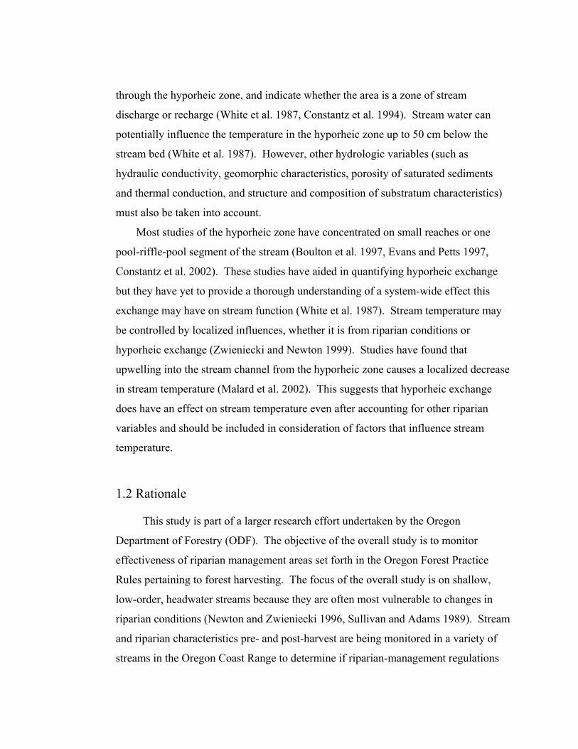
contiguous reaches of greater than 300 m (Figure 2.1). The middle reach (named the
Treatment Reach) varied in length from 300 to 1500 m, depending on the management
plan of the individual landowner. The criterion for the Treatment Reach included a
planned harvest within two years with an actively managed Riparian Management
Area (RMA) in accordance with the Oregon Forest Practice Rules. Upstream and
downstream reaches (the Control Reach and Downstream Reach, respectively) were
each 300 m in length and were to remain un-harvested for the duration of the study
(approximately seven years). These reaches had a minimum buffer width of 60 m of
adjacent vegetation on both sides of the stream, with riparian vegetation greater than
25 years of age. Tracer dilution tests using sodium chloride were conducted on a
subset of four streams representing different temperature patterns during summer low
flow conditions in 2003.
2.1.2 Stream Selection Criteria and Site Descriptions
Site selection resulted in 22 privately owned sites and 16 state-owned sites.
This study consists of 38 streams in the Oregon Coast Range with the southernmost
stream near Coos Bay, Oregon and the northernmost stream near Astoria, Oregon
(Figure 2. 2). Streams in this study were volunteered by landowners with forested
areas that met criteria proposed by ODF. Criteria required stream reaches to be fairly
uniform in riparian characteristics, channel morphology, and stream flow. No major
natural or anthropogenic disturbance was allowed in the study area; therefore there
were no active beaver ponds, recent debris torrents, or dams. This study focused on
Medium Type F (fish bearing streams with flows of 0.06 - 0.28 cms and 1.2 -6.1 m
width), Medium Type N (non-fish bearing streams of the same size) and Small Type F
streams (fish bearing streams with flows of < 0.06 cms and < 1.2 m width) (Logan
2002).
2.2 Stream Characterization Methods
Stream and riparian characteristics were measured every 60 m along the entire
study reach (Control, Treatment, and Downstream) of every stream. Temperature
probes were placed in at least four locations along the stream: the downstream and
upstream end of the study site, at the interface between the reaches, and additionally at
the confluence of any major perennial tributary (Figure 2.1). Characterizations for 21
streams were measured during the summer 2002 and stream temperatures were
monitored for these streams from June to September in 2002 and 2003.
Characterization for 17 streams selected in 2003 was conducted during summer 2003
and stream temperatures were monitored from June to September 2003.
Figure 2.1- Schematic of study design layout for evaluation of stream temperature responses to logging on 38 small headwater streams in the Oregon Coast Range.
Control Reach
Treatment Reach Downstream Reach
Harvest
Temperature Probe
2002 & 2003 RipStream Study Sites
LEGEND
2002 Installed Study Sites
2003 Installed Study Sites
E
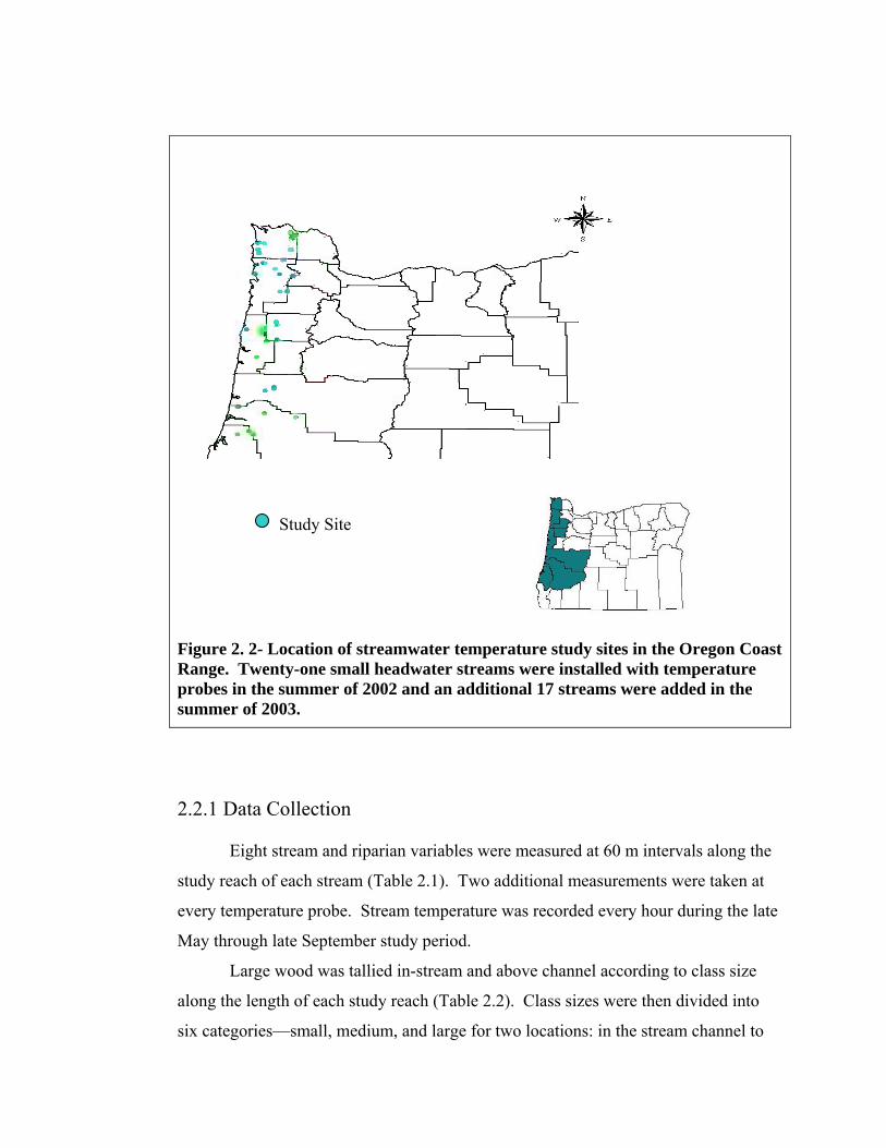
Figure 2. 2- Location of streamwater temperature study sites in the Oregon Coast Range. Twenty-one small headwater streams were installed with temperature probes in the summer of 2002 and an additional 17 streams were added in the summer of 2003.
2.2.1 Data Collection
Eight stream and riparian variables were measured at 60 m intervals along the
study reach of each stream (Table 2.1). Two additional measurements were taken at
every temperature probe. Stream temperature was recorded every hour during the late
May through late September study period.
Large wood was tallied in-stream and above channel according to class size
along the length of each study reach (Table 2.2). Class sizes were then divided into
six categories—small, medium, and large for two locations: in the stream channel to
Study Site
bankfull height, and between bankfull height and 1.8 m above the channel (Table 2.3)
(Welty et al. 2002). This was to determine different locations of large wood and its
influence on stream temperature. Volume and number of wood jams (a grouping of
many pieces of wood too great to count) were also recorded in the field.
A field crew of three measured stream and riparian characteristics and
completed approximately one stream per day. One field member carried the fish-eye
camera and was responsible for taking pictures of the canopy for quantifications of
shade. The second field member tallied large wood as the crew moved along the reach
and was in charge of estimating substrate composition and recording the rest of the
data collected by this individual and the third crew member. The third crew member
carried a hip chain that measures distance and determined where each stream cross
section was to be taken. This individual then flagged a large tree or bush indicating
the location of the transect and aided the second member in collecting the rest of the
data.
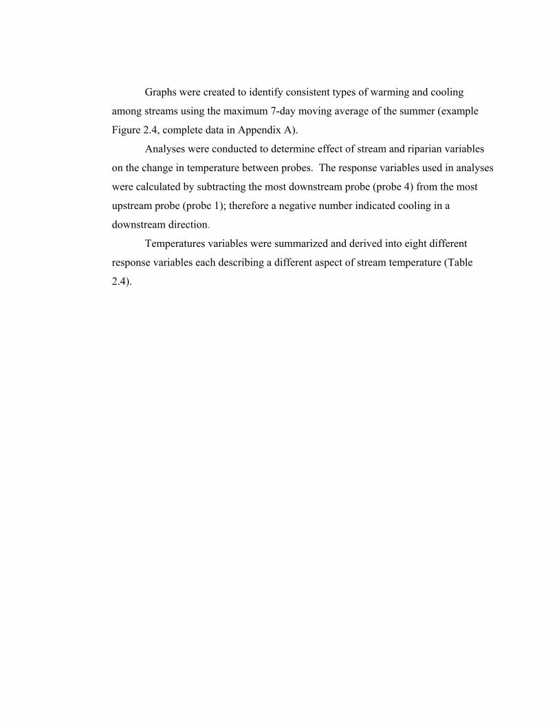
Four additional variables were determined using GIS. The zone of coastal
influence, or the fog zone, was delineated (Figure 2. 3) and sites were determined as
either in the zone of coastal influence or outside its bounds. Two types of geology
dominate in the Coast Range of Oregon and sites were classified accordingly: igneous
and sedimentary. Region of study site was split into North Coast, Middle Coast, and
South Coast and sites were again classified accordingly. Aspect was classified as
North, Northeast, East, Southeast, South, Southwest, West, or Northwest. Stream type
was also a variable in this study and sites were either Small, non-fish-bearing streams
or Medium fish-bearing streams.

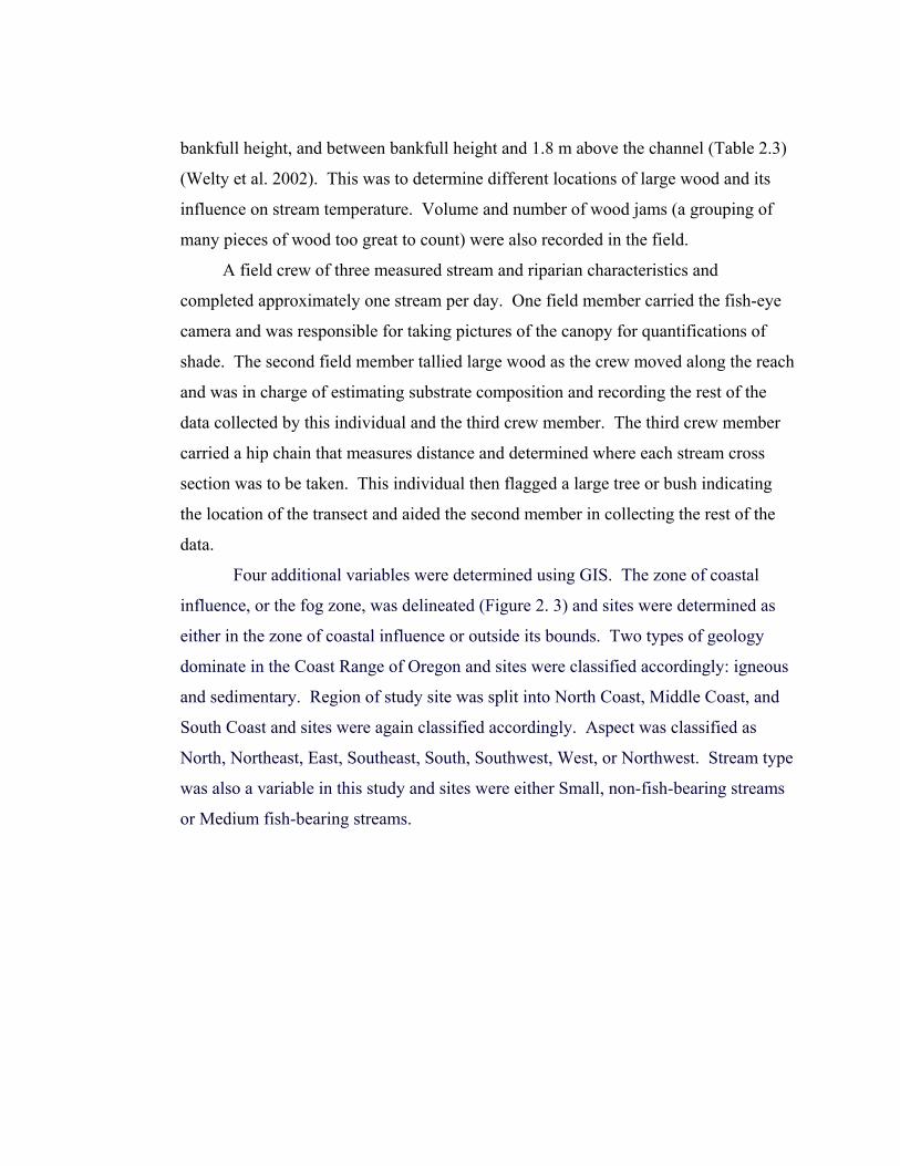
Table 2.1- Stream and riparian variables collected along study reaches in 38 headwater streams in the Oregon Coast Range. Variable measured every 60m DescriptionThalweg Depth The depth of stream water was measured with a flow rod at the deepest point in the channel cross section
Wetted WidthThe width of the wetted surface of the stream was measured at the data collection point with a tape measure. Mid-channel bars that were out of the water were subtracted from the width of the wetted channel.
Bankfull Width
The height of the wetted channel at bankfull flow (average annual peak flow) was estimated and the width of the channel at this estimated height was measured with a tape measure.
Floodprone Width
A measurement was taken at twice the bank full height at the deepest part of the channel cross section. The tape measure was then extended to either side of the channel at this height until an incline was reached which would impede the water or until 20m was reached. The flood plain was estimated if wider than 20m.
Substrate CompostionSubstrate was described as either bedrock, boulder, cobble, gravel or fine material. Estimates of substrate composition were based from these criteria proposed by ODF:Bedrock is solid rock or substrate.Boulders are sized between a car and a basketball.Cobbles are between a basketball and a baseball.Gravel is between a baseball and a ladybug.Fine substrate is smaller than a ladybug.
Gradient
The gradient of the channel was measured from the top of a riffle to the top of the next upstream riffle. Two members of the field crew faced each other and used a clinometer to measure the percent gradient.
Large Wood
Volume of large wood was estimated and tallied along the entire reach of the stream. Two tables were devised for each 60 m section (Table 2.2). The tables divide varying volumes of large wood and tic marks were placed in each table where large wood was observed (Table 2.3). Large wood was divided and tallied in two classifications:
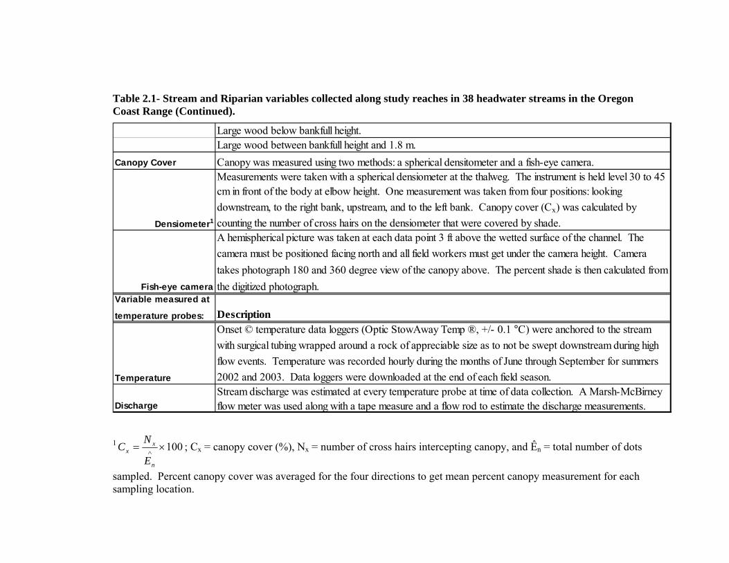
Table 2.1- Stream and Riparian variables collected along study reaches in 38 headwater streams in the Oregon Coast Range (Continued).
Large wood below bankfull height.Large wood between bankfull height and 1.8 m.
Canopy Cover Canopy was measured using two methods: a spherical densitometer and a fish-eye camera.
Densiometer1
Measurements were taken with a spherical densiometer at the thalweg. The instrument is held level 30 to 45 cm in front of the body at elbow height. One measurement was taken from four positions: looking downstream, to the right bank, upstream, and to the left bank. Canopy cover (Cx) was calculated by counting the number of cross hairs on the densiometer that were covered by shade.
Fish-eye camera
A hemispherical picture was taken at each data point 3 ft above the wetted surface of the channel. The camera must be positioned facing north and all field workers must get under the camera height. Camera takes photograph 180 and 360 degree view of the canopy above. The percent shade is then calculated from the digitized photograph.
Variable measured at
temperature probes: Description
Temperature
Onset © temperature data loggers (Optic StowAway Temp ®, +/- 0.1 °C) were anchored to the stream with surgical tubing wrapped around a rock of appreciable size as to not be swept downstream during high flow events. Temperature was recorded hourly during the months of June through September for summers 2002 and 2003. Data loggers were downloaded at the end of each field season.
DischargeStream discharge was estimated at every temperature probe at time of data collection. A Marsh-McBirney flow meter was used along with a tape measure and a flow rod to estimate the discharge measurements.
1 100×= ∧
n
xx
E
NC ; Cx = canopy cover (%), Nx = number of cross hairs intercepting canopy, and Ên = total number of dots
sampled. Percent canopy cover was averaged for the four directions to get mean percent canopy measurement for each sampling location.
Table 2.2- Example of data sheet for tally of wood pieces along stream channels in small streams in the Oregon Coast Range. Small, medium, and large wood classifications were derived from these tallies.
Site Name: Beeches CR Channel Segment Number: 400-600 Wood Pieces Partially or Small End
Completely within the BFW1
Diameter Length (m) (cm) 1.5-3 (m) 3.1-6.2 (m) 6.3-9 (m) >9 (m) 12.2-26 II III II 26.1-46 I 46.1-62 62.1-92 I >92 Site Name: Beeches CR Channel Segment Number: 400-600 Wood Pieces Partially or Completely Small End
within the BFW between BFD2 and 1.8 m.
Diameter Length (m) (cm) 1.5-3 (m) 3.1-6.2 (m) 6.3-9 (m) >9 (m) 12.2-26 I 26.1-46 III II 46.1-62 I 62.1-92 >92 I Wood Jams Number Height
(m) Width (m) Length
(m)
I 1.5 3 6
1BFW= Bankfull width 2BFD= Bankfull depth
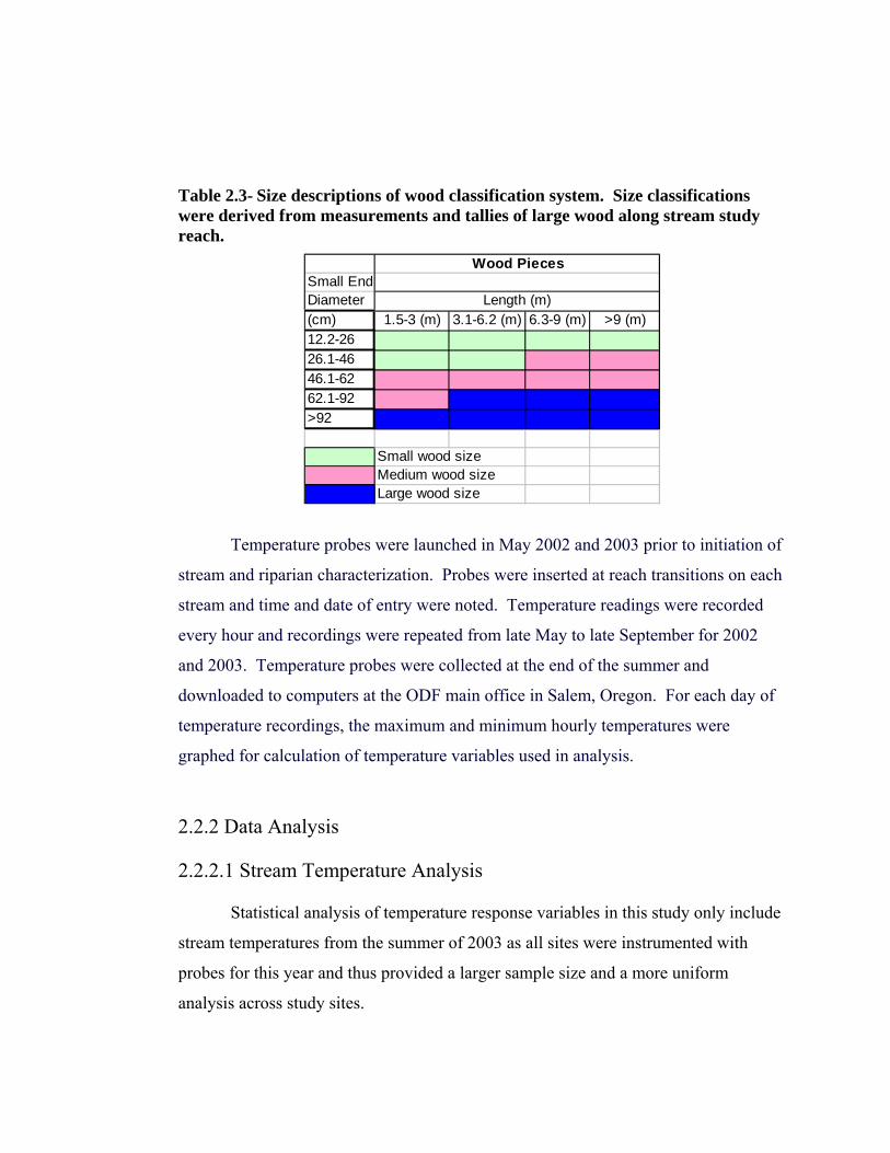
Table 2.3- Size descriptions of wood classification system. Size classifications were derived from measurements and tallies of large wood along stream study reach.
Small End Diameter(cm) 1.5-3 (m) 3.1-6.2 (m) 6.3-9 (m) >9 (m)12.2-2626.1-4646.1-6262.1-92>92
Small wood sizeMedium wood sizeLarge wood size
Wood Pieces
Length (m)
Temperature probes were launched in May 2002 and 2003 prior to initiation of
stream and riparian characterization. Probes were inserted at reach transitions on each
stream and time and date of entry were noted. Temperature readings were recorded
every hour and recordings were repeated from late May to late September for 2002
and 2003. Temperature probes were collected at the end of the summer and
downloaded to computers at the ODF main office in Salem, Oregon. For each day of
temperature recordings, the maximum and minimum hourly temperatures were
graphed for calculation of temperature variables used in analysis.
2.2.2 Data Analysis
2.2.2.1 Stream Temperature Analysis
Statistical analysis of temperature response variables in this study only include
stream temperatures from the summer of 2003 as all sites were instrumented with
probes for this year and thus provided a larger sample size and a more uniform
analysis across study sites.
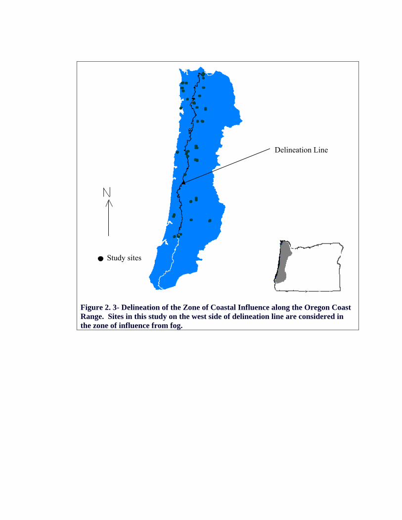
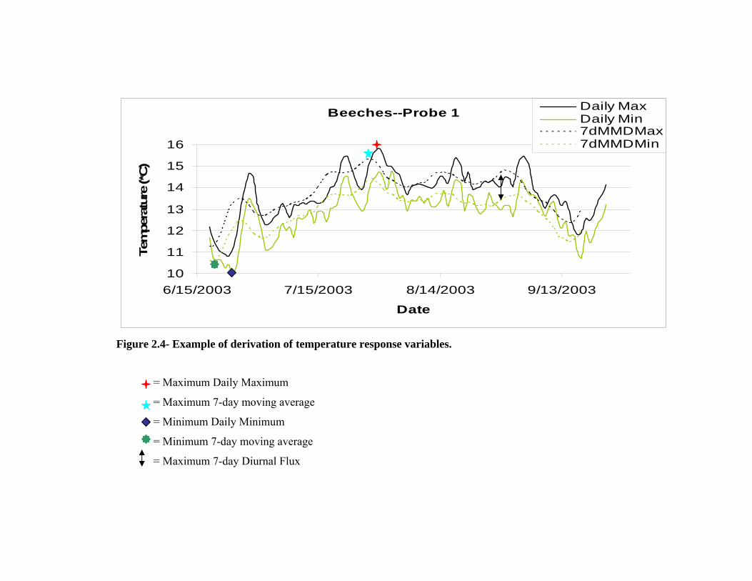
Graphs were created to identify consistent types of warming and cooling
among streams using the maximum 7-day moving average of the summer (example
Figure 2.4, complete data in Appendix A).
Analyses were conducted to determine effect of stream and riparian variables
on the change in temperature between probes. The response variables used in analyses
were calculated by subtracting the most downstream probe (probe 4) from the most
upstream probe (probe 1); therefore a negative number indicated cooling in a
downstream direction.
Temperatures variables were summarized and derived into eight different
response variables each describing a different aspect of stream temperature (Table
2.4).
N a.
S.us
I
Figure 2. 3- Delineation of the Zone of Coastal Influence along the Oregon Coast Range. Sites in this study on the west side of delineation line are considered in the zone of influence from fog.
Delineation Line
Study sites
Beeches--Probe 1
10
11
12
13
14
15
16
6/15/2003 7/15/2003 8/14/2003 9/13/2003
Date
Tem
pera
ture
(*C
)
Daily MaxDaily Min7dMMDMax7dMMDMin
Figure 2.4- Example of derivation of temperature response variables.
= Maximum Daily Maximum
= Maximum 7-day moving average
= Minimum Daily Minimum
= Minimum 7-day moving average
= Maximum 7-day Diurnal Flux

Table 2. 4- Stream temperature responses used in analysis with stream and riparian variables. Two abbreviations indicate summarizations of stream
temperature that were used in deriving temperature responses for analysis. A description of the temperature response and how it was derived is provided. Abbreviation Description7dMMDMax 7-day moving average of daily maximum temperatures.7dMMDMin 7-day moving average of daily minimum temperatures.Temperaure Response Description
Max7d
Average of the summertime maximum of the 7-day moving mean of the daily maximum of probes two, three, and four. All probes analyzed using the same hottest week based on probe 4 of each site.
DiffMax7dMax
Difference between probe 4 and probe 1 of the Maximum summer 7dMMDMax. The warmest 7-day period of the summer. All probes analyzed using the same hottest week based on probe 4 of each site.
DiffMaxDailyMax
Difference between probe 4 and probe 1 of the Maximum Daily Maximum temperature of the summer. This day was determined using the hottest day of the summer from probe 4, then this day was used for the "hottest" day for the other probes. Process was repeated for each site.
DiffAve7dMax
Difference between probe 4 and probe 1 of the average of
the 7dMMDMax’s of the summer.
DiffMin7dMin
Difference between probe 4 and probe 1 of the Minimum summer 7dMMDMin. The coldest 7-day period of the summer. All probes analyzed using the same coldest week based on probe 4.
DiffMinDailyMin
Difference between probe 4 and probe 1 of the Minimum Daily Minimum temperature of the summer. This day was determined using the coldest day of the summer from probe 4, then this day was used for the "coldest" day for the other probes.
DiffAve7dMin
Difference between probe 4 and probe 1 of the average of the 7dMMDMin’s of the summer.
DiffMax7dDiFlux
Difference between probe 4 and probe 1 of the Maximum 7-day Diurnal Flux. The 7-day period of the greatest daily change in temperature.

2.2.2.2 Relationships between stream temperature and independent variables
A selection process to determine the most appropriate model for each response
variable in relation to stream and riparian variables was implemented. Data were
analyzed four ways: (1) using the average of all measurements of stream and riparian
characteristics along a particular stream, or splitting these descriptive characteristics
into (2) all Control Reaches, (3) all Treatment Reaches, and (4) all Downstream
Reaches. For each of the above four types of stream and riparian descriptions, simple
linear regressions were first tested between each of the eight temperature response
variables and each of 17 stream and riparian characteristics using S-Plus. Significant
variables (p < 0.05) were then considered and regressed again with each of the 17
stream characteristics until the best fitting model was found. Model selection was
determined by significant p-values and high R2’s (models with R2’s closer to 1.00
were considered more significant). Models either had one, two, or three descriptive
variables. This is a type of manual stepwise regression to determine the best model.
This selection process was used as a result of the high number of explanatory variables
we wanted to consider. By conducting the stepwise regression manually, no violations
of this statistical method occurred.
As a check to see if variables chosen in this process of model selection were
the “best fit” model, an alternative model selection process was cross-checked with the
manual stepwise regression. Akaike’s Information Criterion (AIC) was applied to
models with more than one significant independent variable accounting for variation
in temperature response. Lewis et al. (1999) also used this method to determine
significant explanatory variables for stream temperature. The equation used to
determine the AIC for each model is:
pnAIC 2)log( 2 +×= σ [Eq. 2]
where n = number of streams, σ2 = the residual mean square (read from the S-Plus
output), and p = number of explanatory variables in the model. This equation
measures the goodness of fit of each individual model and includes a penalty for the
number of terms in a model. Therefore, as opposed to evaluations of R2’s, goodness
of fit does not necessarily increase with the number of terms in the model.
The hottest week of the summer for each study site was also analyzed and
compared to characteristics of the streams measured in this study. The hottest week of
the summer was first graphed with the maximum 7-day period of the summer to
determine what dates had the warmest stream temperatures in this study, as this
temperature variable is used most often in evaluating effects of forest practices and for
summarization of temperature in small streams in Oregon. Hottest week was then
compared to variables thought to contribute to timing of maximum temperatures.
Variables such as geology, region, and aspect were considered here.
2.3 Tracer Dilution Methods
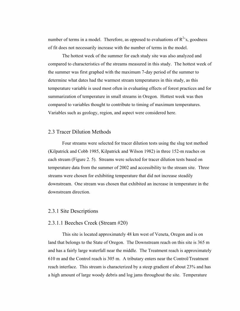
Four streams were selected for tracer dilution tests using the slug test method
(Kilpatrick and Cobb 1985, Kilpatrick and Wilson 1982) in three 152-m reaches on
each stream (Figure 2. 5). Streams were selected for tracer dilution tests based on
temperature data from the summer of 2002 and accessibility to the stream site. Three
streams were chosen for exhibiting temperature that did not increase steadily
downstream. One stream was chosen that exhibited an increase in temperature in the
downstream direction.
2.3.1 Site Descriptions
2.3.1.1 Beeches Creek (Stream #20)
This site is located approximately 48 km west of Veneta, Oregon and is on
land that belongs to the State of Oregon. The Downstream reach on this site is 365 m
and has a fairly large waterfall near the middle. The Treatment reach is approximately
610 m and the Control reach is 305 m. A tributary enters near the Control/Treatment
reach interface. This stream is characterized by a steep gradient of about 23% and has
a high amount of large woody debris and log jams throughout the site. Temperature

decreased over the length of the study reach and this stream was chosen for its
complexity of wood and channel morphology and relatively steep gradient.
2.3.1.2 Nettle Meyer (Stream #6) This site is located approximately 72 km west of Portland, Oregon on lands
that belong to the State of Oregon. This site is characterized by a fairly even mix of
cobble, gravel, and fine substrate and has a slight incline with an average gradient of
approximately 3%. The Downstream, Treatment, and Control reaches are all 305 m in
length. Temperature increases steadily in a downstream direction at this site. Channel
characteristics are relatively uniform, with a minimum amount of large wood,
meandering, or unusually steep gradients.
2.3.1.3 Ice Box (Stream #9)
This site is located 3 km south of Cannon Beach, Oregon on Weyerhaeuser
Company property. The study site is 1005 m. There is no Downstream reach on this
stream and therefore there are only three temperature probes for this site. There is a
culvert approximately 245 m upstream of probe #3 (downstream end of the Treatment
Reach). Below this culvert the stream is very steep and is dominated by boulders and
large wood. Above the culvert the stream is very flat with a primarily gravel substrate
and a minimum of wood. The culvert and complete change of channel characteristics
made this site unique. In addition, the middle temperature probe on this stream was
significantly warmer than the probe above and below, indicating warming followed by
subsequent cooling.
2.3.1.4 Toad Creek (Stream #12) This site is located approximately 80 km west of Portland, Oregon on
Longview Fibre property. This site is characterized by mostly large boulders, cobble,
and bedrock. The Control reach (305 m) is mostly bedrock and is located above two
S
fairly significant waterfalls. The Downstream reach (305 m) has a culvert and a road
crossing that splits it in two. The Treatment reach is approximately 915 m. Average
gradient on this reach is approximately 8%. This stream was chosen because it
displayed overall cooling but high variability through the study reach in the summer
2002, with the second probe warmer than the first, the third probe the coolest of them
all, and the fourth temperature probe warmer than the third. Temperature patterns on
this stream warranted further investigation.
Figure 2. 5- Location of four sites subjected to tracer tests in the summer of 2003. Sites had varying stream and riparian characteristics and
displayed different patterns of stream warming.
2.3.2 Data Collection For tracer dilution tests, a Campbell Scientific CR-10 data logger and
conductivity probe was placed near a previously installed temperature probe. The
Location of tracer study
sites Study sites
#20
#6#12
#9
conductivity probe was cleaned before each test and calibrated to each stream.
Calibration involved a known salt concentration and water from the stream to be
tested. A known volume of stream water was placed into a bucket and conductivity
was measured by inserting the probe. Known volumes of a calibration solution were
then inserted into the bucket and the increasing conductivity of the bucket water was
recorded to confirm calibration. Using this method, the CR-10 was checked at each
new stream for accurate readings of conductivity and adjusted when necessary.
After cleaning the conductivity probe again and placing it in the stream water
near the temperature probe, the data collection program was transferred to the CR-10
using the software PConnect and a Palm Pilot. The program designed for this
experiment took readings of streamwater conductivity every 5 seconds. Every minute,
two readings were recorded: an average of readings for the entire minute and a random
sample of conductivity from a 5-second interval within the minute. The minute-
recording was repeated until the experiment was concluded and the battery
disconnected. The program had to be transferred to the CR-10 every time the battery
was reconnected using a Palm Pilot and serial cable. The battery only operated by
connecting with the red wire prior to the black wire. The experiment was considered
“complete” when conductivity of the stream water was within 10% of the original
conductivity (Kilpatrick and Cobb 1985). At the conclusion of the test the Palm Pilot
was reconnected to the CR-10 and the data uploaded to the Palm Pilot. Data were then
transferred from the Palm Pilot to a laptop or desktop computer.
Once the data logger was launched, I attached a hip chain or string box to my
belt and walked approximately 152 m upstream. A known amount of sodium chloride
(Hi-Grade Iodized Evaporated Salt) was dumped (or “slugged”) into the stream,
preferably at a location in the stream that was swift moving to maximize mixing. The
CR-10 recorded streamwater conductivity and length of the test was determined by the
amount of time it took streamwater to return to pre-slug conditions.
A test length of 152 m was carried out on all streams (Figure 2.6). This was a
somewhat arbitrary reach length chosen to estimate and characterize the residence
time of water in these small headwater streams. A longer reach length was not
suitable for this study as flows were very low in most of these streams and completion
of tests would have taken too long. Shorter reach lengths were not chosen because we
did not feel a shorter reach would encompass enough of the complexity of these small
streams to get an accurate estimate of residence time over a reach length relevant to
our study.
Three tracer tests were performed on each of the four streams: (1) 152 m above
the Downstream probe (#4), (2) the probe at the bottom of the Treatment Reach (#3),
(3) and the probe at the bottom of the Control Reach (#2) (Figure 2.6). Stream and
riparian characterization data were not collected for the 152 m above the upstream
probe (#1) as this reach was not always accessible and was therefore not measured.
Tracer tests were performed in an upstream direction to ensure than no salt from a
previous experiment confounded a current experiment. If tracer tests had to be redone
on a particular stream or reach, a few days were allowed between the tests to ensure
that all salt from previous experiments had been washed out of the stream. Quantities
of salt were determined separately for each stream reach and were added to the
reaches in amounts ranging from 3,000 g to 6,000 g (Table 2.6).
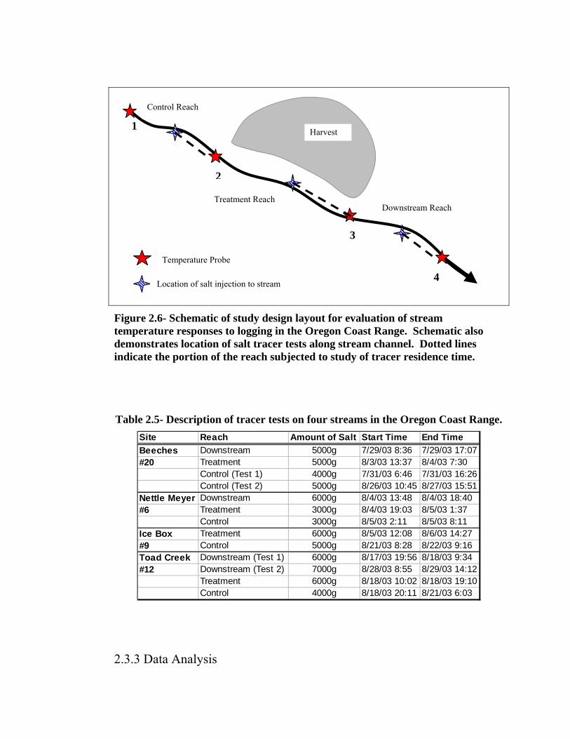
Figure 2.6- Schematic of study design layout for evaluation of stream temperature responses to logging in the Oregon Coast Range. Schematic also demonstrates location of salt tracer tests along stream channel. Dotted lines indicate the portion of the reach subjected to study of tracer residence time.
Table 2.5- Description of tracer tests on four streams in the Oregon Coast Range. Site Reach Amount of Salt Start Time End TimeBeeches Downstream 5000g 7/29/03 8:36 7/29/03 17:07#20 Treatment 5000g 8/3/03 13:37 8/4/03 7:30
Control (Test 1) 4000g 7/31/03 6:46 7/31/03 16:26Control (Test 2) 5000g 8/26/03 10:45 8/27/03 15:51
Nettle Meyer Downstream 6000g 8/4/03 13:48 8/4/03 18:40#6 Treatment 3000g 8/4/03 19:03 8/5/03 1:37
Control 3000g 8/5/03 2:11 8/5/03 8:11Ice Box Treatment 6000g 8/5/03 12:08 8/6/03 14:27#9 Control 5000g 8/21/03 8:28 8/22/03 9:16Toad Creek Downstream (Test 1) 6000g 8/17/03 19:56 8/18/03 9:34#12 Downstream (Test 2) 7000g 8/28/03 8:55 8/29/03 14:12
Treatment 6000g 8/18/03 10:02 8/18/03 19:10Control 4000g 8/18/03 20:11 8/21/03 6:03
2.3.3 Data Analysis
Control Reach
Treatment Reach Downstream Reach
Harvest
Temperature Probe
Location of salt injection to stream
1
2
3
4
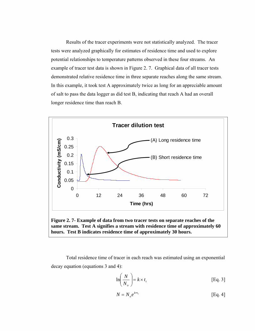
Results of the tracer experiments were not statistically analyzed. The tracer
tests were analyzed graphically for estimates of residence time and used to explore
potential relationships to temperature patterns observed in these four streams. An
example of tracer test data is shown in Figure 2. 7. Graphical data of all tracer tests
demonstrated relative residence time in three separate reaches along the same stream.
In this example, it took test A approximately twice as long for an appreciable amount
of salt to pass the data logger as did test B, indicating that reach A had an overall
longer residence time than reach B.
Tracer dilution test
0
0.05
0.1
0.15
0.2
0.25
0.3
0 12 24 36 48 60 72
Time (hrs)
Con
duct
ivity
(mS/
cm) (A) Long residence time
(B) Short residence time
Figure 2. 7- Example of data from two tracer tests on separate reaches of the same stream. Test A signifies a stream with residence time of approximately 60 hours. Test B indicates residence time of approximately 30 hours.
Total residence time of tracer in each reach was estimated using an exponential
decay equation (equations 3 and 4):
to
tkNN
×=⎟⎟⎠
⎞⎜⎜⎝
⎛ln [Eq. 3]
rtkoeNN ∗= [Eq. 4]

where N = conductivity at time of termination of test, No = conductivity of the stream
at the peak of the test, tt = observed test time, k = decay constant derived using
equation 3. The calculated decay constant, k, is used in equation 4 to solve for tr,
residence time. This calculation was done to confirm estimates of residence time from
in-field measurements.

Chapter III
Results
3.1 Stream Temperature Characteristics
3.1.1 Stream and Riparian Characteristics
Bankfull width varied from 1.6 to 8.1 m with a mean of 4.3 m and a standard
deviation of 1.5 m (Figure 3. 1). Channel steepness ranged from 1% to 22% with a
mean of 7.5% and a standard deviation of 4.7 % (Figure 3. 2). Flood-prone width
varied from 5.4 to 39.2 m with a mean of 10.6 m (median 8.9 m) and a standard
deviation of 5.7 m (Figure 3. 3). Average percent canopy cover using the densiometer
ranged from 69.4% to 96.6%, with a mean of 92.1% and a standard deviation of 5.1 %
(Figure 3. 4). Percent bedrock ranged from 0% to 34.5% (mean = 5%, standard
deviation = 8%), percent boulder ranged from 0% to 17.5% (mean = 4%, standard
deviation = 5%), percent cobble ranged from 0% to 42.9% (mean = 18%, standard
deviation = 11%), percent gravel ranged from 2.4% to 58.3% (mean = 38%, standard
deviation = 11%), and percent fine substrate ranged from 6.7% to 97.6% (mean =
35%, standard deviation = 20%) (Figure 3. 5). Tallies of large wood sizes and
numbers ranged from absence of a particular size of wood per 100 m to 13.2 pieces of
wood per 100 m (Table 3. 1).
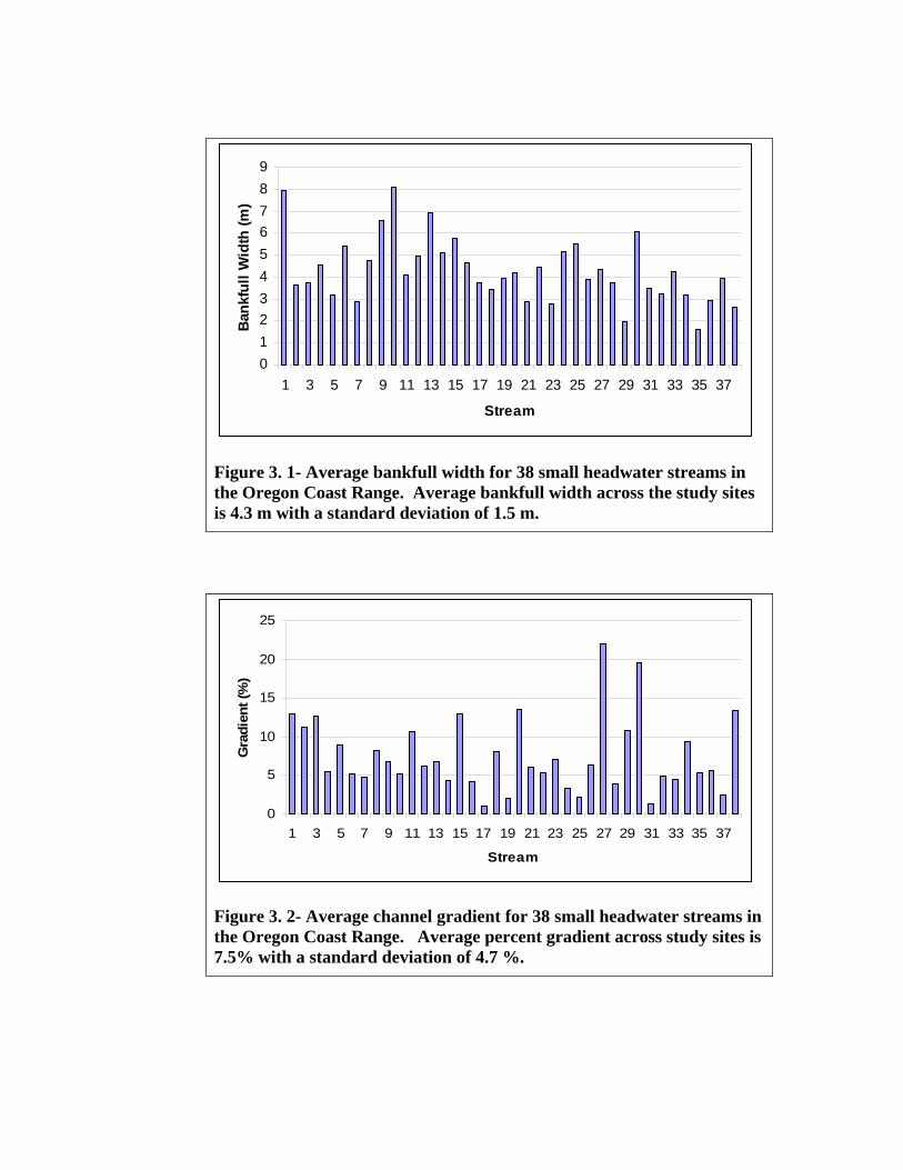
0123456789
1 3 5 7 9 11 13 15 17 19 21 23 25 27 29 31 33 35 37
Stream
Ban
kful
l Wid
th (m
)
Figure 3. 1- Average bankfull width for 38 small headwater streams in the Oregon Coast Range. Average bankfull width across the study sites is 4.3 m with a standard deviation of 1.5 m.
0
5
10
15
20
25
1 3 5 7 9 11 13 15 17 19 21 23 25 27 29 31 33 35 37
Stream
Gra
dien
t (%
)
Figure 3. 2- Average channel gradient for 38 small headwater streams in the Oregon Coast Range. Average percent gradient across study sites is 7.5% with a standard deviation of 4.7 %.

05
1015202530354045
1 3 5 7 9 11 13 15 17 19 21 23 25 27 29 31 33 35 37
Stream
Floo
d-pr
one
wid
th (m
)
Figure 3. 3- Average width of flood-prone valley in 38 small headwater streams in the Oregon Coast Range. Average FPW is 10.6 m (median of 8.9 m) with a standard deviation of 5.7 m.
60
70
80
90
100
0 2 4 6 8 10 12 14 16 18 20 22 24 26 28 30 32 34 36 38
Stream
Cano
py C
over
(%)
Figure 3. 4- Average canopy cover of 38 small headwater streams in the Oregon Coast Range. Average canopy cover in study sites is 92.1% with a standard deviation of 5.1 %.
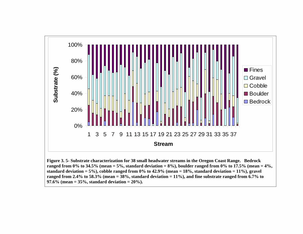
0%
20%
40%
60%
80%
100%
1 3 5 7 9 11 13 15 17 19 21 23 25 27 29 31 33 35 37
Stream
Subs
trat
e (%
) FinesGravelCobbleBoulderBedrock
Figure 3. 5- Substrate characterization for 38 small headwater streams in the Oregon Coast Range. Bedrock ranged from 0% to 34.5% (mean = 5%, standard deviation = 8%), boulder ranged from 0% to 17.5% (mean = 4%, standard deviation = 5%), cobble ranged from 0% to 42.9% (mean = 18%, standard deviation = 11%), gravel ranged from 2.4% to 58.3% (mean = 38%, standard deviation = 11%), and fine substrate ranged from 6.7% to 97.6% (mean = 35%, standard deviation = 20%).
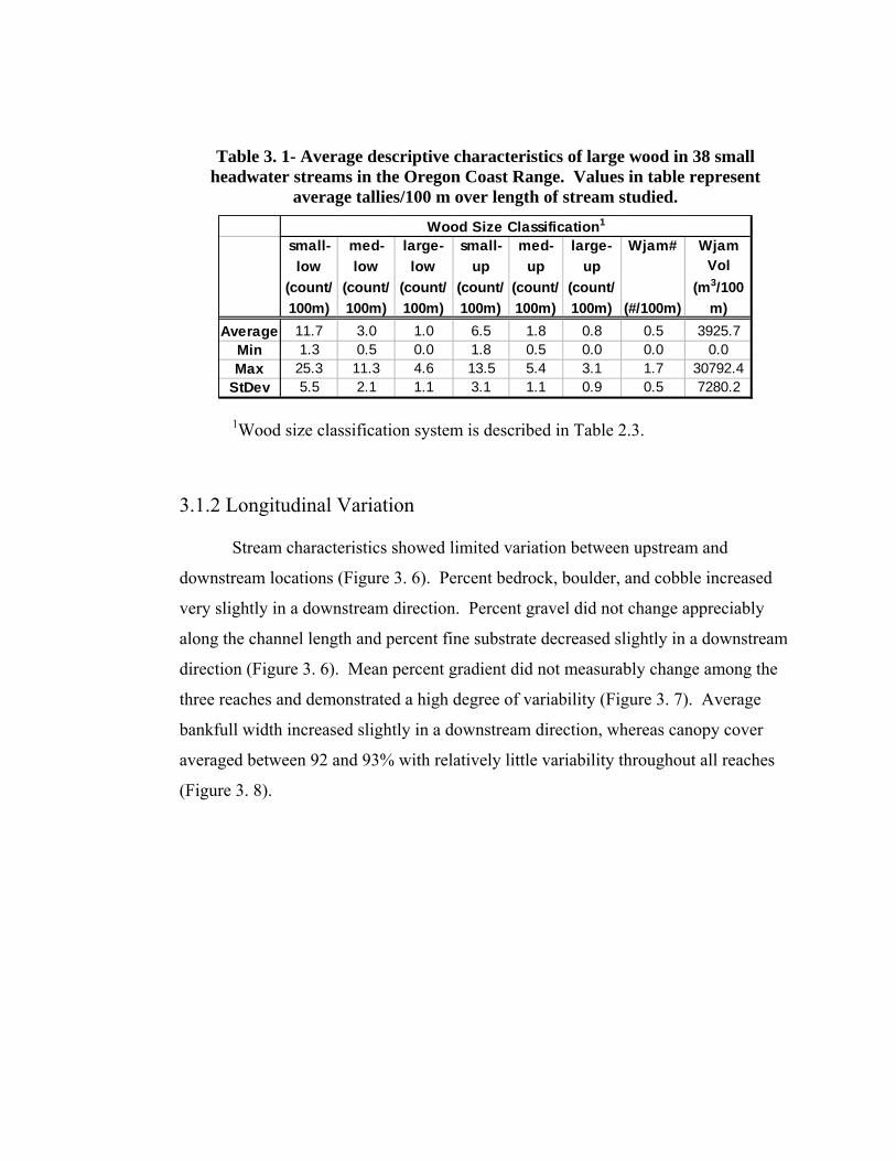
Table 3. 1- Average descriptive characteristics of large wood in 38 small headwater streams in the Oregon Coast Range. Values in table represent
average tallies/100 m over length of stream studied.
small-low
(count/100m)
med- low
(count/100m)
large- low
(count/100m)
small-up
(count/100m)
med-up
(count/100m)
large- up
(count/100m)
Wjam#
(#/100m)
Wjam Vol
(m3/100m)
Average 11.7 3.0 1.0 6.5 1.8 0.8 0.5 3925.7Min 1.3 0.5 0.0 1.8 0.5 0.0 0.0 0.0Max 25.3 11.3 4.6 13.5 5.4 3.1 1.7 30792.4
StDev 5.5 2.1 1.1 3.1 1.1 0.9 0.5 7280.2
Wood Size Classification1
1Wood size classification system is described in Table 2.3.
3.1.2 Longitudinal Variation
Stream characteristics showed limited variation between upstream and
downstream locations (Figure 3. 6). Percent bedrock, boulder, and cobble increased
very slightly in a downstream direction. Percent gravel did not change appreciably
along the channel length and percent fine substrate decreased slightly in a downstream
direction (Figure 3. 6). Mean percent gradient did not measurably change among the
three reaches and demonstrated a high degree of variability (Figure 3. 7). Average
bankfull width increased slightly in a downstream direction, whereas canopy cover
averaged between 92 and 93% with relatively little variability throughout all reaches
(Figure 3. 8).
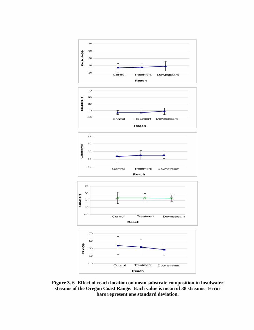
DownstreamTreatmentControl-10
10
30
50
70
ReachBed
rock
(%)
DownstreamTreatmentControl-10
10
30
50
70
Reach
Bou
lder
(%)
DownstreamTreatmentControl-10
10
30
50
70
Reach
Cob
ble (%
)
DownstreamTreatmentControl-10
10
30
50
70
Reach
Gra
vel (%
)
Control Treatment Downstream-10
10
30
50
70
Reach
Fine
(%)
Figure 3. 6- Effect of reach location on mean substrate composition in headwater streams of the Oregon Coast Range. Each value is mean of 38 streams. Error
bars represent one standard deviation.
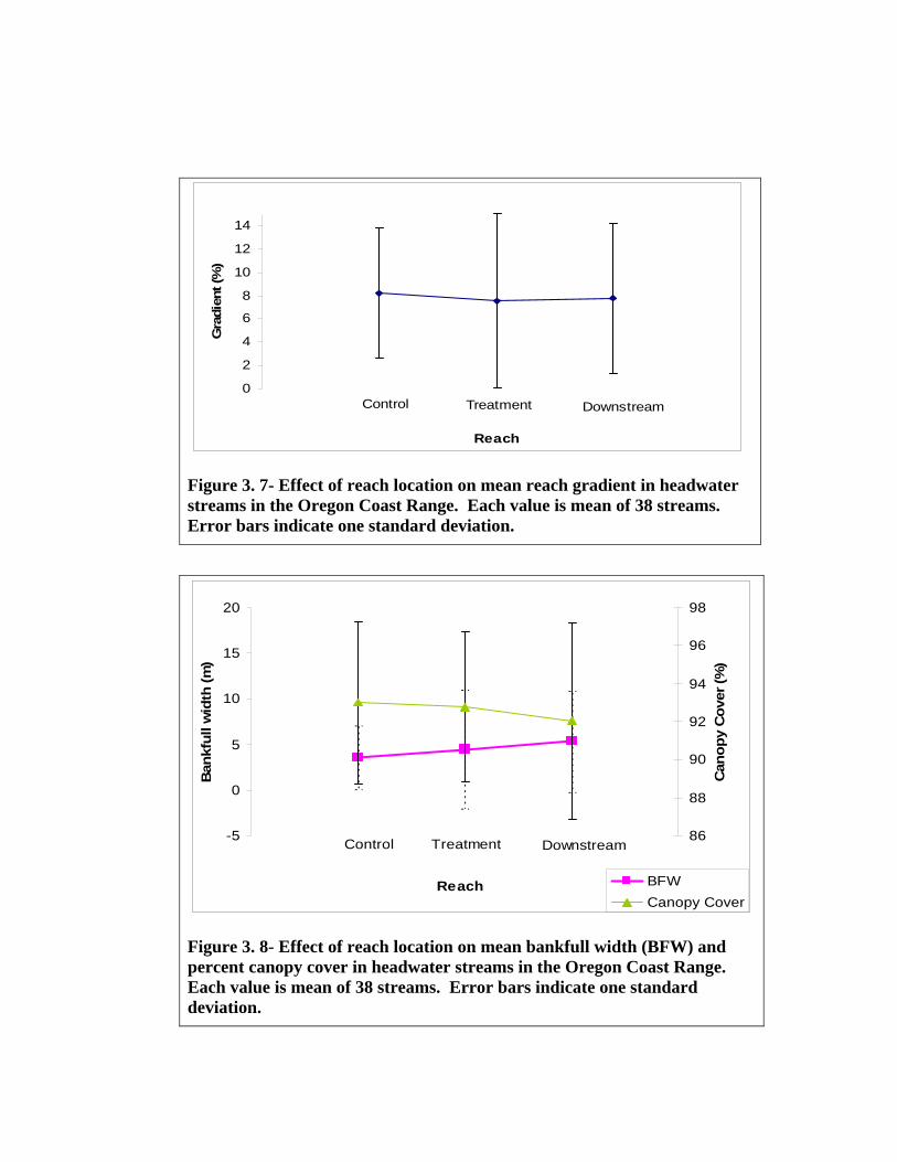
DownstreamTreatmentControl0
2
4
6
8
10
12
14
Reach
Gra
dien
t (%
)
Figure 3. 7- Effect of reach location on mean reach gradient in headwater streams in the Oregon Coast Range. Each value is mean of 38 streams. Error bars indicate one standard deviation.
DownstreamTreatmentControl-5
0
5
10
15
20
Reach
Ban
kful
l wid
th (m
)
86
88
90
92
94
96
98
Can
opy
Cov
er (%
)
BFWCanopy Cover
Figure 3. 8- Effect of reach location on mean bankfull width (BFW) and percent canopy cover in headwater streams in the Oregon Coast Range. Each value is mean of 38 streams. Error bars indicate one standard deviation.
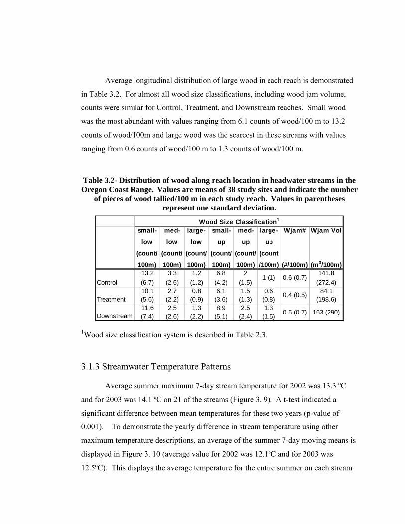
Average longitudinal distribution of large wood in each reach is demonstrated
in Table 3.2. For almost all wood size classifications, including wood jam volume,
counts were similar for Control, Treatment, and Downstream reaches. Small wood
was the most abundant with values ranging from 6.1 counts of wood/100 m to 13.2
counts of wood/100m and large wood was the scarcest in these streams with values
ranging from 0.6 counts of wood/100 m to 1.3 counts of wood/100 m.
Table 3.2- Distribution of wood along reach location in headwater streams in the Oregon Coast Range. Values are means of 38 study sites and indicate the number
of pieces of wood tallied/100 m in each study reach. Values in parentheses represent one standard deviation.
small-
low
(count/
100m)
med-
low
(count/
100m)
large-
low
(count/
100m)
small-
up
(count/
100m)
med-
up
(count/
100m)
large-
up
(count
/100m)
Wjam#
(#/100m)
Wjam Vol
(m3/100m)
Control13.2 (6.7)
3.3 (2.6)
1.2 (1.2)
6.8 (4.2)
2 (1.5)
1 (1) 0.6 (0.7)141.8
(272.4)
Treatment10.1 (5.6)
2.7 (2.2)
0.8 (0.9)
6.1 (3.6)
1.5 (1.3)
0.6 (0.8)
0.4 (0.5) 84.1 (198.6)
Downstream11.6 (7.4)
2.5 (2.6)
1.3 (2.2)
8.9 (5.1)
2.5 (2.4)
1.3 (1.5)
0.5 (0.7) 163 (290)
Wood Size Classification1
1Wood size classification system is described in Table 2.3.
3.1.3 Streamwater Temperature Patterns
Average summer maximum 7-day stream temperature for 2002 was 13.3 ºC
and for 2003 was 14.1 ºC on 21 of the streams (Figure 3. 9). A t-test indicated a
significant difference between mean temperatures for these two years (p-value of
0.001). To demonstrate the yearly difference in stream temperature using other
maximum temperature descriptions, an average of the summer 7-day moving means is
displayed in Figure 3. 10 (average value for 2002 was 12.1ºC and for 2003 was
12.5ºC). This displays the average temperature for the entire summer on each stream
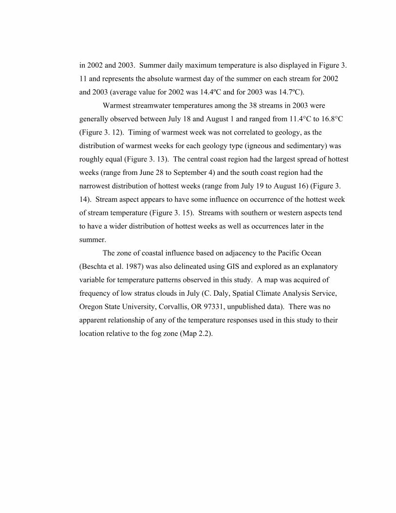
in 2002 and 2003. Summer daily maximum temperature is also displayed in Figure 3.
11 and represents the absolute warmest day of the summer on each stream for 2002
and 2003 (average value for 2002 was 14.4ºC and for 2003 was 14.7ºC).
Warmest streamwater temperatures among the 38 streams in 2003 were
generally observed between July 18 and August 1 and ranged from 11.4°C to 16.8°C
(Figure 3. 12). Timing of warmest week was not correlated to geology, as the
distribution of warmest weeks for each geology type (igneous and sedimentary) was
roughly equal (Figure 3. 13). The central coast region had the largest spread of hottest
weeks (range from June 28 to September 4) and the south coast region had the
narrowest distribution of hottest weeks (range from July 19 to August 16) (Figure 3.
14). Stream aspect appears to have some influence on occurrence of the hottest week
of stream temperature (Figure 3. 15). Streams with southern or western aspects tend
to have a wider distribution of hottest weeks as well as occurrences later in the
summer.
The zone of coastal influence based on adjacency to the Pacific Ocean
(Beschta et al. 1987) was also delineated using GIS and explored as an explanatory
variable for temperature patterns observed in this study. A map was acquired of
frequency of low stratus clouds in July (C. Daly, Spatial Climate Analysis Service,
Oregon State University, Corvallis, OR 97331, unpublished data). There was no
apparent relationship of any of the temperature responses used in this study to their
location relative to the fog zone (Map 2.2).
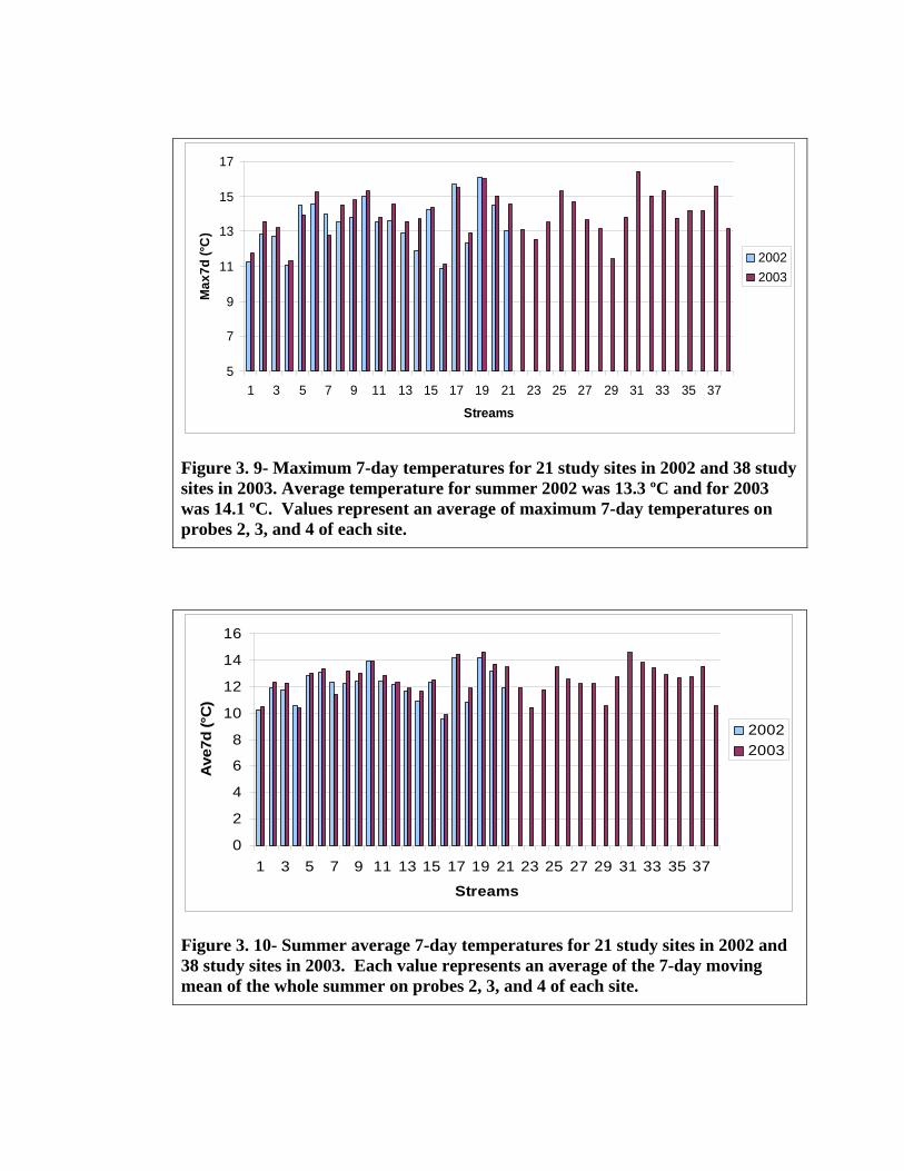
5
7
9
11
13
15
17
1 3 5 7 9 11 13 15 17 19 21 23 25 27 29 31 33 35 37
Streams
Max
7d (°
C)
20022003
Figure 3. 9- Maximum 7-day temperatures for 21 study sites in 2002 and 38 study sites in 2003. Average temperature for summer 2002 was 13.3 ºC and for 2003 was 14.1 ºC. Values represent an average of maximum 7-day temperatures on probes 2, 3, and 4 of each site.
0
2
4
6
8
10
12
14
16
1 3 5 7 9 11 13 15 17 19 21 23 25 27 29 31 33 35 37
Streams
Ave
7d (°
C)
20022003
Figure 3. 10- Summer average 7-day temperatures for 21 study sites in 2002 and 38 study sites in 2003. Each value represents an average of the 7-day moving mean of the whole summer on probes 2, 3, and 4 of each site.
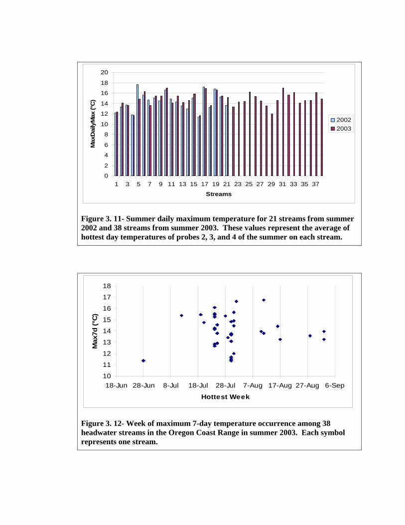
0
2
4
6
8
10
12
14
16
18
20
1 3 5 7 9 11 13 15 17 19 21 23 25 27 29 31 33 35 37
Streams
Max
Dai
lyM
ax (°
C)
20022003
Figure 3. 11- Summer daily maximum temperature for 21 streams from summer 2002 and 38 streams from summer 2003. These values represent the average of hottest day temperatures of probes 2, 3, and 4 of the summer on each stream.
10
11
12
13
14
15
16
17
18
18-Jun 28-Jun 8-Jul 18-Jul 28-Jul 7-Aug 17-Aug 27-Aug 6-Sep
Hottest Week
Max
7d (°
C)
Figure 3. 12- Week of maximum 7-day temperature occurrence among 38 headwater streams in the Oregon Coast Range in summer 2003. Each symbol represents one stream.

18-Jun
28-Jun
8-Jul
18-Jul
28-Jul
7-Aug
17-Aug
27-Aug
6-Sep
Geology
Hot
test
Wee
k
Figure 3. 13- Effect of geologic substrate on occurrence of maximum 7-day temperature among 38 headwater streams in the Oregon Coast Range in summer 2003. Each symbol represents one stream.
18-Jun
28-Jun
8-Jul
18-Jul
28-Jul
7-Aug
17-Aug
27-Aug
6-Sep
Region
Hot
test
Wee
k
Figure 3. 14- Effect of regional location on occurrence of maximum 7-day temperature among 38 headwater streams in the Oregon Coast Range. Each symbol represents one stream.
North Coast Central Coast South Coast
Igneous Sedimentary
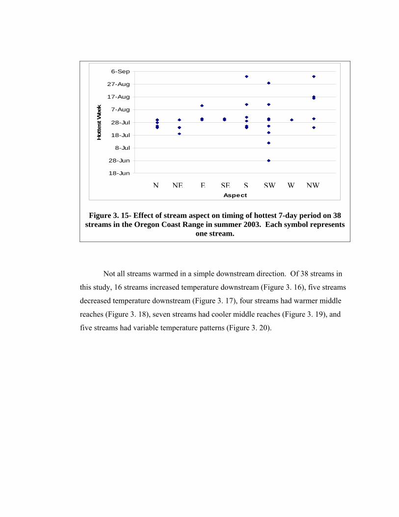
18-Jun
28-Jun
8-Jul
18-Jul
28-Jul
7-Aug
17-Aug
27-Aug
6-Sep
Aspect
Hot
test
Wee
k
Figure 3. 15- Effect of stream aspect on timing of hottest 7-day period on 38 streams in the Oregon Coast Range in summer 2003. Each symbol represents
one stream.
Not all streams warmed in a simple downstream direction. Of 38 streams in
this study, 16 streams increased temperature downstream (Figure 3. 16), five streams
decreased temperature downstream (Figure 3. 17), four streams had warmer middle
reaches (Figure 3. 18), seven streams had cooler middle reaches (Figure 3. 19), and
five streams had variable temperature patterns (Figure 3. 20).
N NE E SE S SW W NW
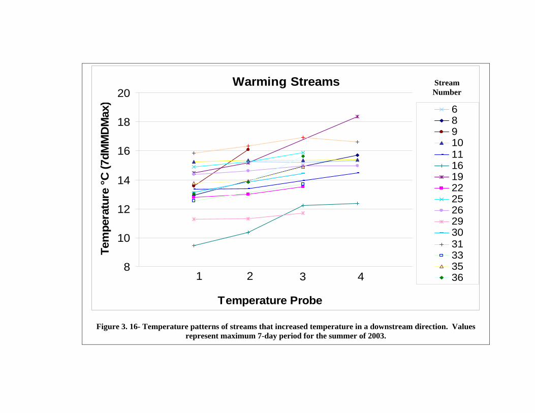
Warming Streams
431 28
10
12
14
16
18
20
Temperature Probe
Tem
pera
ture
°C (7
dMM
DM
ax)
68910111619222526293031333536
Figure 3. 16- Temperature patterns of streams that increased temperature in a downstream direction. Values represent maximum 7-day period for the summer of 2003.
Stream Number
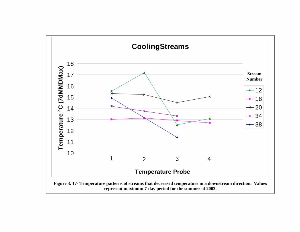
CoolingStreams
432110
11
12
13
14
15
16
17
18
Temperature Probe
Tem
pera
ture
°C (7
dMM
DM
ax)
1218203438
Figure 3. 17- Temperature patterns of streams that decreased temperature in a downstream direction. Values represent maximum 7-day period for the summer of 2003.
Stream Number

Warm Middle Reaches
1 2 3 410
11
12
13
14
15
Temperature Probe
Tem
pera
ture
°C (7
dMM
DM
ax)
13
1315
Figure 3. 18- Patterns of stream temperature with warm middle reaches. Values represent maximum 7-day period for the summer of 2003.
Stream Number
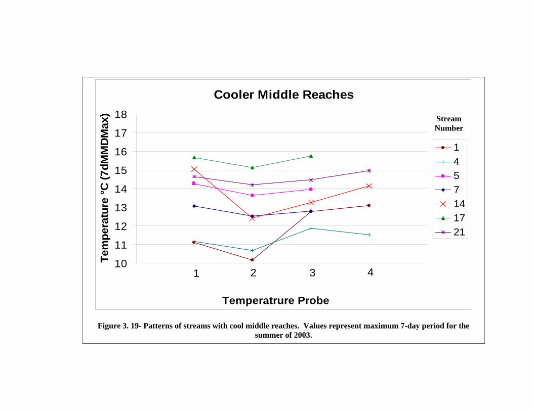
Cooler Middle Reaches
432110
11
12
13
14
15
16
17
18
Temperatrure Probe
Tem
pera
ture
°C (7
dMM
DM
ax)
1457141721
Figure 3. 19- Patterns of streams with cool middle reaches. Values represent maximum 7-day period for the summer of 2003.
Stream Number
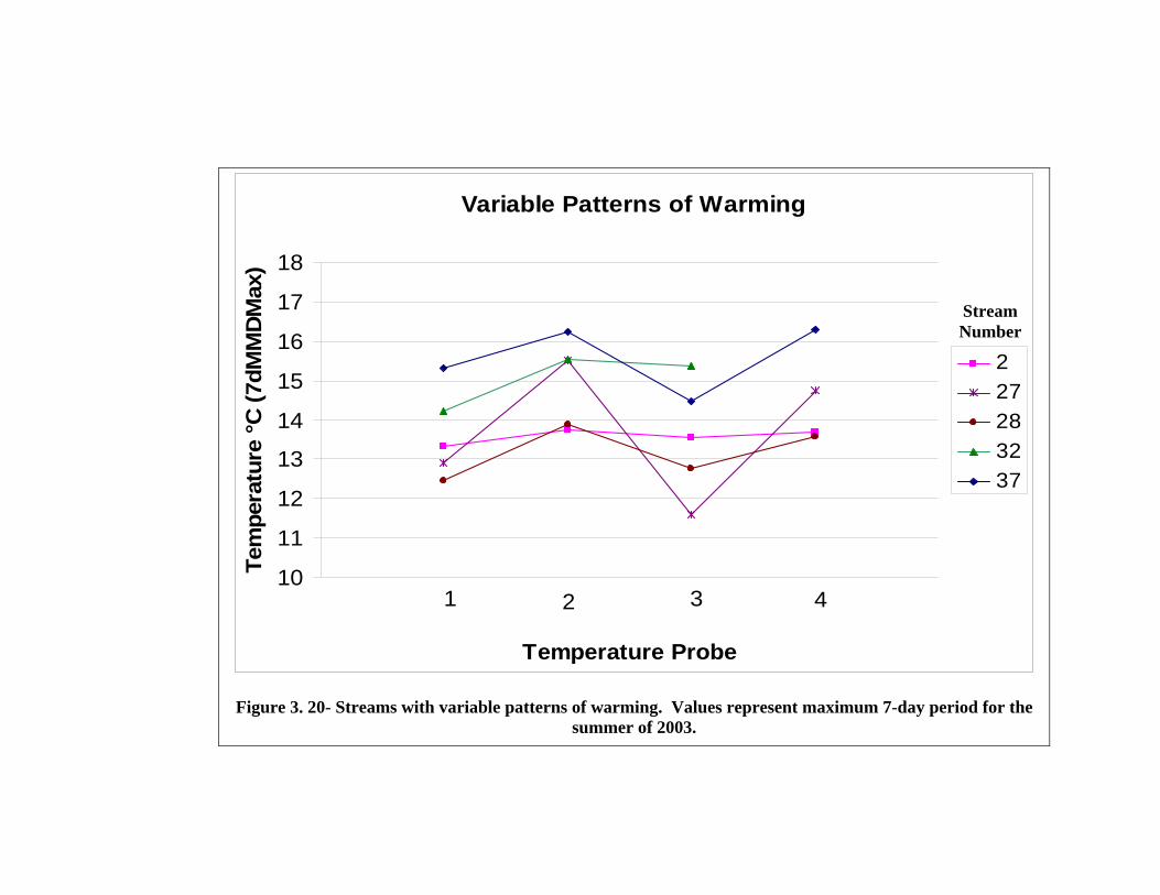
Variable Patterns of Warming
432110
11
12
13
14
15
16
17
18
Temperature Probe
Tem
pera
ture
°C
(7dM
MD
Max
)
227283237
Figure 3. 20- Streams with variable patterns of warming. Values represent maximum 7-day period for the summer of 2003.
Stream Number
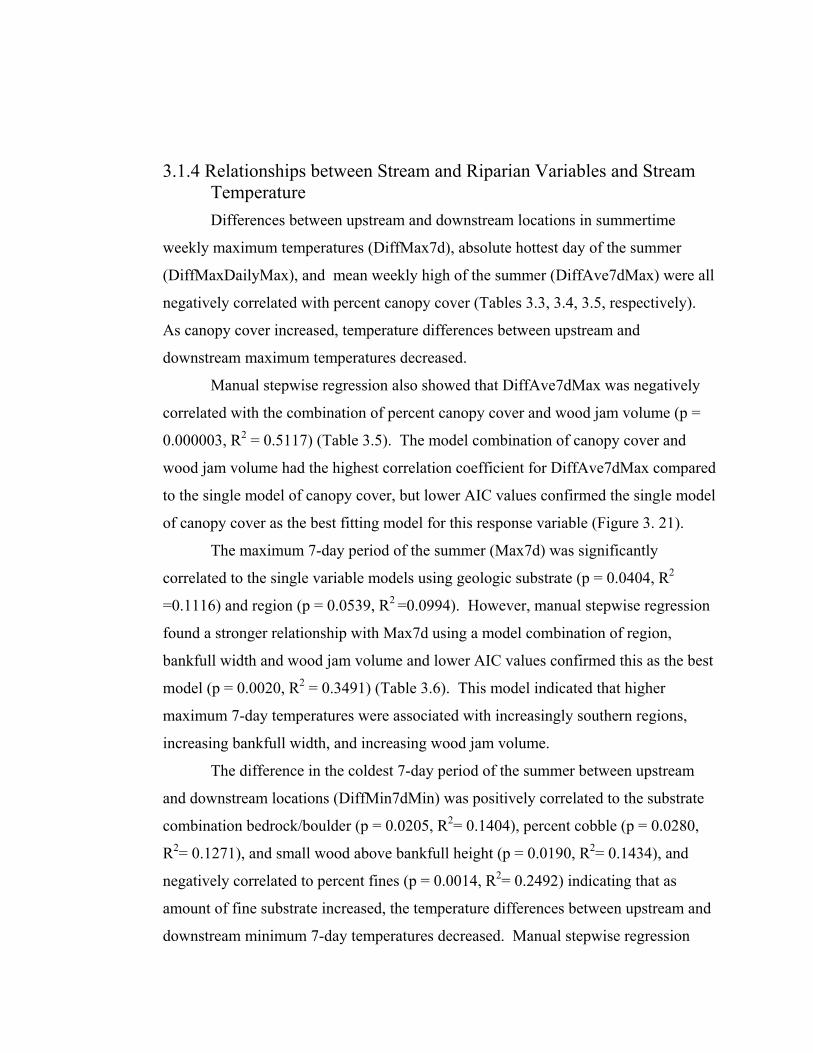
3.1.4 Relationships between Stream and Riparian Variables and Stream Temperature
Differences between upstream and downstream locations in summertime
weekly maximum temperatures (DiffMax7d), absolute hottest day of the summer
(DiffMaxDailyMax), and mean weekly high of the summer (DiffAve7dMax) were all
negatively correlated with percent canopy cover (Tables 3.3, 3.4, 3.5, respectively).
As canopy cover increased, temperature differences between upstream and
downstream maximum temperatures decreased.
Manual stepwise regression also showed that DiffAve7dMax was negatively
correlated with the combination of percent canopy cover and wood jam volume (p =
0.000003, R2 = 0.5117) (Table 3.5). The model combination of canopy cover and
wood jam volume had the highest correlation coefficient for DiffAve7dMax compared
to the single model of canopy cover, but lower AIC values confirmed the single model
of canopy cover as the best fitting model for this response variable (Figure 3. 21).
The maximum 7-day period of the summer (Max7d) was significantly
correlated to the single variable models using geologic substrate (p = 0.0404, R2
=0.1116) and region (p = 0.0539, R2 =0.0994). However, manual stepwise regression
found a stronger relationship with Max7d using a model combination of region,
bankfull width and wood jam volume and lower AIC values confirmed this as the best
model (p = 0.0020, R2 = 0.3491) (Table 3.6). This model indicated that higher
maximum 7-day temperatures were associated with increasingly southern regions,
increasing bankfull width, and increasing wood jam volume.
The difference in the coldest 7-day period of the summer between upstream
and downstream locations (DiffMin7dMin) was positively correlated to the substrate
combination bedrock/boulder (p = 0.0205, R2= 0.1404), percent cobble (p = 0.0280,
R2= 0.1271), and small wood above bankfull height (p = 0.0190, R2= 0.1434), and
negatively correlated to percent fines (p = 0.0014, R2= 0.2492) indicating that as
amount of fine substrate increased, the temperature differences between upstream and
downstream minimum 7-day temperatures decreased. Manual stepwise regression
also identified a positive relationship between DiffMin7dMin and the combination of
small wood above bankfull height and bedrock/boulder (p = 0.0065, R2= 0.2500).
However, AIC values indicated fine substrate as the best fitting model for this
temperature response (Table 3. 7).
Difference in the coldest daily minimum of the summer between upstream and
downstream locations (DiffMinDailyMin) was negatively correlated with single
variable models using geologic substrate (p = 0.0061, R= 0.1911), region (p = 0.0146,
R2 = 0.1545), and percent canopy (p = 0.0404, R2 = 0.1116) (Table 3. 8). Manual
stepwise regression identified the combination of geology and canopy cover in relation
to DiffMinDailyMin with the highest correlation coefficient and lowest AIC. As
geology changed from igneous to sedimentary and canopy cover decreased,
differences between upstream and downstream minimum daily temperatures
decreased.
The difference in the mean weekly low of the summer between upstream and
downstream locations (DiffAve7dMin) was not significantly correlated with any of the
variables measured in this study (Table 3. 9). The difference in the 7-day period of the
greatest daily change in temperature between upstream and downstream locations
(DiffMax7dDiFlux) was negatively correlated with canopy cover (p = 0.02, R2 =
0.1491) (Table 3.10).
y = -0.12x + 11.726R2 = 0.4544
p = 0.0
-2.0
-1.0
0.0
1.0
2.0
3.0
4.0
60 65 70 75 80 85 90 95 100
Canopy Cover (%)
DiffA
ve7d
Max
(°C)
Figure 3. 21- Relationship between canopy cover and change in average 7-day maximum temperatures between upstream and downstream locations during 2003 in 38 headwater streams in the Oregon Coast Range. Each symbol represents one stream.
p = 0.0000
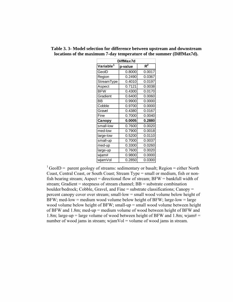
Table 3. 3- Model selection for difference between upstream and downstream locations of the maximum 7-day temperature of the summer (DiffMax7d).
Variable1 p-value R2
GeoID 0.8000 0.0017Region 0.2490 0.0367StreamType 0.4010 0.0197Aspect 0.7121 0.0038BFW 0.4300 0.0170Gradient 0.6400 0.0060BB 0.9900 0.0000Cobble 0.9700 0.0000Gravel 0.4380 0.0167Fine 0.7000 0.0040Canopy 0.0005 0.2880small-low 0.7600 0.0020med-low 0.7900 0.0018large-low 0.5200 0.0110small-up 0.7000 0.0037med-up 0.3300 0.0260large-up 0.7600 0.0020wjam# 0.9800 0.0000wjamVol 0.2850 0.0300
DiffMax7d
1 GeoID = parent geology of streams: sedimentary or basalt; Region = either North Coast, Central Coast, or South Coast; Stream Type = small or medium, fish or non-fish bearing stream; Aspect = directional flow of stream; BFW = bankfull width of stream; Gradient = steepness of stream channel; BB = substrate combination boulder/bedrock; Cobble, Gravel, and Fine = substrate classifications; Canopy = percent canopy cover over stream; small-low = small wood volume below height of BFW; med-low = medium wood volume below height of BFW; large-low = large wood volume below height of BFW; small-up = small wood volume between height of BFW and 1.8m; med-up = medium volume of wood between height of BFW and 1.8m; large-up = large volume of wood between height of BFW and 1.8m; wjam# = number of wood jams in stream; wjamVol = volume of wood jams in stream.
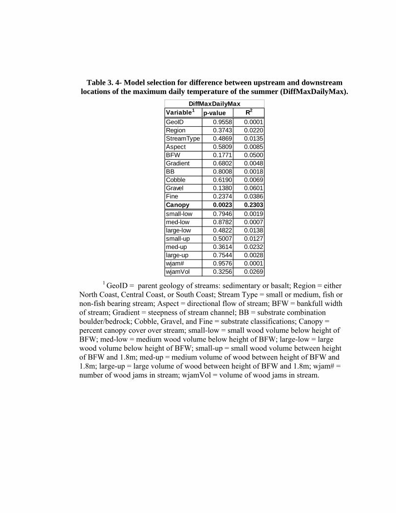
Table 3. 4- Model selection for difference between upstream and downstream locations of the maximum daily temperature of the summer (DiffMaxDailyMax).
Variable1 p-value R2
GeoID 0.9558 0.0001Region 0.3743 0.0220StreamType 0.4869 0.0135Aspect 0.5809 0.0085BFW 0.1771 0.0500Gradient 0.6802 0.0048BB 0.8008 0.0018Cobble 0.6190 0.0069Gravel 0.1380 0.0601Fine 0.2374 0.0386Canopy 0.0023 0.2303small-low 0.7946 0.0019med-low 0.8782 0.0007large-low 0.4822 0.0138small-up 0.5007 0.0127med-up 0.3614 0.0232large-up 0.7544 0.0028wjam# 0.9576 0.0001wjamVol 0.3256 0.0269
DiffMaxDailyMax
1 GeoID = parent geology of streams: sedimentary or basalt; Region = either North Coast, Central Coast, or South Coast; Stream Type = small or medium, fish or non-fish bearing stream; Aspect = directional flow of stream; BFW = bankfull width of stream; Gradient = steepness of stream channel; BB = substrate combination boulder/bedrock; Cobble, Gravel, and Fine = substrate classifications; Canopy = percent canopy cover over stream; small-low = small wood volume below height of BFW; med-low = medium wood volume below height of BFW; large-low = large wood volume below height of BFW; small-up = small wood volume between height of BFW and 1.8m; med-up = medium volume of wood between height of BFW and 1.8m; large-up = large volume of wood between height of BFW and 1.8m; wjam# = number of wood jams in stream; wjamVol = volume of wood jams in stream.
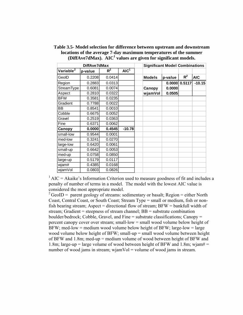
Table 3.5- Model selection for difference between upstream and downstream locations of the average 7-day maximum temperatures of the summer
(DiffAve7dMax). AIC1 values are given for significant models. Significant Model Combinations
Variable2 p-value R2 AIC1
GeoID 0.2208 0.0414 Models p-value R2 AICRegion 0.2883 0.0313 0.0000 0.5117 -10.15StreamType 0.6081 0.0074 Canopy 0.0000Aspect 0.2810 0.0322 wjamVol 0.0505BFW 0.3581 0.0235Gradient 0.7788 0.0022BB 0.8541 0.0010Cobble 0.6675 0.0052Gravel 0.2519 0.0363Fine 0.6371 0.0062Canopy 0.0000 0.4545 -10.78small-low 0.9544 0.0001med-low 0.3241 0.0270large-low 0.6420 0.0061small-up 0.6642 0.0053med-up 0.0758 0.0850large-up 0.5179 0.0117wjam# 0.4385 0.0168wjamVol 0.0803 0.0826
DiffAve7dMax
1 AIC = Akaike’s Information Criterion used to measure goodness of fit and includes a penalty of number of terms in a model. The model with the lowest AIC value is considered the most appropriate model. 2 GeoID = parent geology of streams: sedimentary or basalt; Region = either North Coast, Central Coast, or South Coast; Stream Type = small or medium, fish or non-fish bearing stream; Aspect = directional flow of stream; BFW = bankfull width of stream; Gradient = steepness of stream channel; BB = substrate combination boulder/bedrock; Cobble, Gravel, and Fine = substrate classifications; Canopy = percent canopy cover over stream; small-low = small wood volume below height of BFW; med-low = medium wood volume below height of BFW; large-low = large wood volume below height of BFW; small-up = small wood volume between height of BFW and 1.8m; med-up = medium volume of wood between height of BFW and 1.8m; large-up = large volume of wood between height of BFW and 1.8m; wjam# = number of wood jams in stream; wjamVol = volume of wood jams in stream.
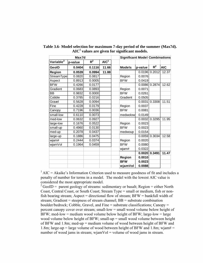
Table 3.6- Model selection for maximum 7-day period of the summer (Max7d). AIC1 values are given for significant models.
Significant Model CombinationsVariable2 p-value R2 AIC1
GeoID 0.0404 0.1116 11.66 Models p-value R2 AICRegion 0.0539 0.0994 11.88 0.0196 0.2012 12.37StreamType 0.0820 0.0817 Region 0.0076Aspect 0.8913 0.0005 BFW 0.0419BFW 0.4266 0.0177 0.0086 0.2874 12.62Gradient 0.0683 0.0893 Region 0.0071BB 0.9832 0.0000 BFW 0.0261Cobble 0.3785 0.0216 Gradient 0.0505Gravel 0.5628 0.0094 0.0031 0.3308 11.51Fine 0.4228 0.0179 Region 0.0037Canopy 0.7196 0.0036 BFW 0.0081small-low 0.6110 0.0073 medwolow 0.0149med-low 0.0632 0.0927 0.0032 0.3295 11.95large-low 0.1676 0.0522 Region 0.0023small-up 0.4960 0.0130 BFW 0.0023med-up 0.2078 0.0437 medwoup 0.0154large-up 0.1886 0.0475 0.0059 0.3034 12.58wjam# 0.2444 0.0374 Region 0.0020wjamVol 0.1964 0.0459 BFW 0.0080
wjam# 0.03220.0020 0.3491 11.47
Region 0.0010BFW 0.0023wjamVol 0.0088
Max7d
1 AIC = Akaike’s Information Criterion used to measure goodness of fit and includes a penalty of number for terms in a model. The model with the lowest AIC value is considered the most appropriate model. 2 GeoID = parent geology of streams: sedimentary or basalt; Region = either North Coast, Central Coast, or South Coast; Stream Type = small or medium, fish or non-fish bearing stream; Aspect = directional flow of stream; BFW = bankfull width of stream; Gradient = steepness of stream channel; BB = substrate combination boulder/bedrock; Cobble, Gravel, and Fine = substrate classifications; Canopy = percent canopy cover over stream; small-low = small wood volume below height of BFW; med-low = medium wood volume below height of BFW; large-low = large wood volume below height of BFW; small-up = small wood volume between height of BFW and 1.8m; med-up = medium volume of wood between height of BFW and 1.8m; large-up = large volume of wood between height of BFW and 1.8m; wjam# = number of wood jams in stream; wjamVol = volume of wood jams in stream.
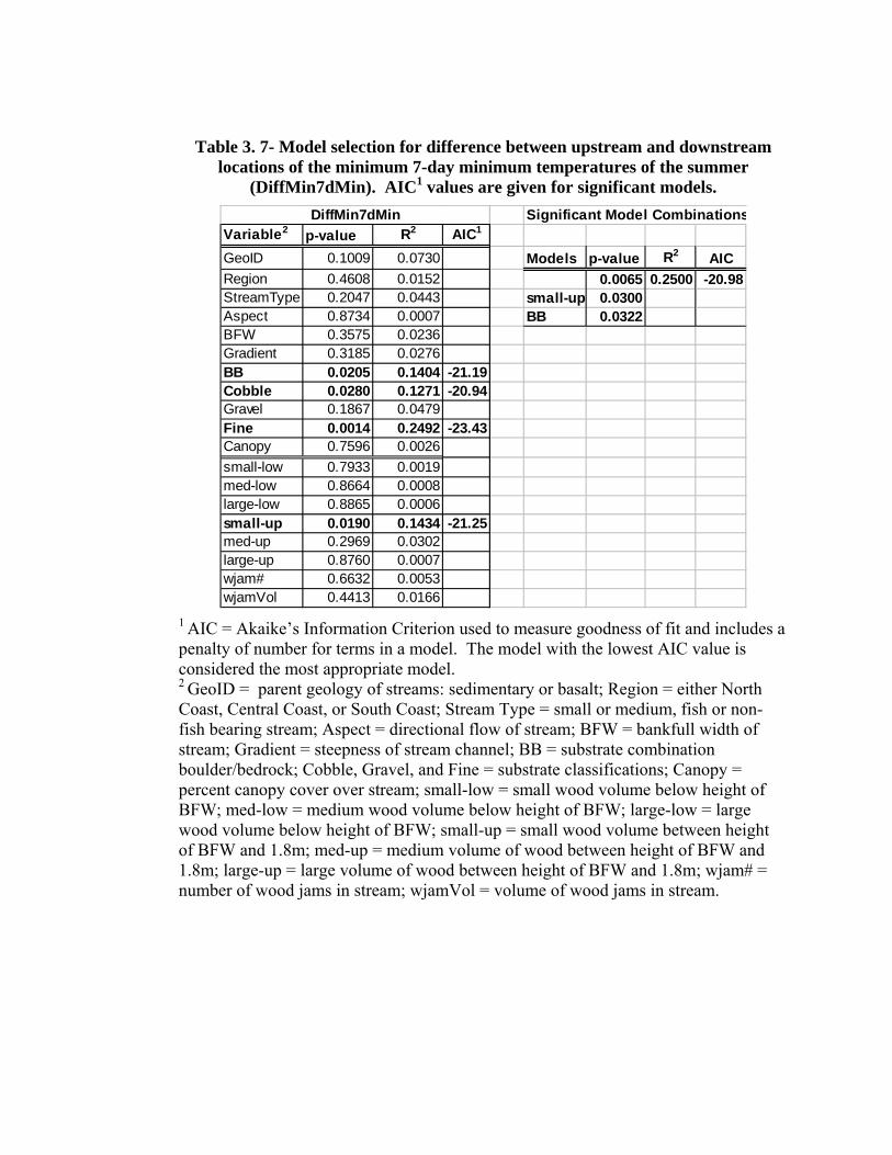
Table 3. 7- Model selection for difference between upstream and downstream locations of the minimum 7-day minimum temperatures of the summer
(DiffMin7dMin). AIC1 values are given for significant models. Significant Model Combinations
Variable2 p-value R2 AIC1
GeoID 0.1009 0.0730 Models p-value R2 AICRegion 0.4608 0.0152 0.0065 0.2500 -20.98StreamType 0.2047 0.0443 small-up 0.0300Aspect 0.8734 0.0007 BB 0.0322BFW 0.3575 0.0236Gradient 0.3185 0.0276BB 0.0205 0.1404 -21.19Cobble 0.0280 0.1271 -20.94Gravel 0.1867 0.0479Fine 0.0014 0.2492 -23.43Canopy 0.7596 0.0026small-low 0.7933 0.0019med-low 0.8664 0.0008large-low 0.8865 0.0006small-up 0.0190 0.1434 -21.25med-up 0.2969 0.0302large-up 0.8760 0.0007wjam# 0.6632 0.0053wjamVol 0.4413 0.0166
DiffMin7dMin
1 AIC = Akaike’s Information Criterion used to measure goodness of fit and includes a penalty of number for terms in a model. The model with the lowest AIC value is considered the most appropriate model. 2 GeoID = parent geology of streams: sedimentary or basalt; Region = either North Coast, Central Coast, or South Coast; Stream Type = small or medium, fish or non-fish bearing stream; Aspect = directional flow of stream; BFW = bankfull width of stream; Gradient = steepness of stream channel; BB = substrate combination boulder/bedrock; Cobble, Gravel, and Fine = substrate classifications; Canopy = percent canopy cover over stream; small-low = small wood volume below height of BFW; med-low = medium wood volume below height of BFW; large-low = large wood volume below height of BFW; small-up = small wood volume between height of BFW and 1.8m; med-up = medium volume of wood between height of BFW and 1.8m; large-up = large volume of wood between height of BFW and 1.8m; wjam# = number of wood jams in stream; wjamVol = volume of wood jams in stream.

Table 3. 8- Model selection for difference between upstream and downstream locations of the minimum daily temperature of the summer (DiffMinDailyMin).
AIC1 values are given for significant models. Significant Model Combination
Variable2 p-value R2 AIC1
GeoID 0.0061 0.1911 -5.9700 Models p-value R2 AICRegion 0.0146 0.1545 -5.2300 0.0005 0.3547 -7.23StreamType 0.1963 0.0459 GeoID 0.0009Aspect 0.1289 0.0629 Canopy 0.0052BFW 0.7493 0.0029Gradient 0.7599 0.0026BB 0.7319 0.0033Cobble 0.4803 0.0139Gravel 0.4135 0.0187Fine 0.3242 0.0270Canopy 0.0404 0.1116 -4.4200small-low 0.7161 0.0037med-low 0.5354 0.0108large-low 0.9215 0.0003small-up 0.3036 0.0294med-up 0.5398 0.0105large-up 0.7117 0.0038wjam# 0.9767 0.0000wjamVol 0.7558 0.0027
DiffMinDailyMin
1 AIC = Akaike’s Information Criterion used to measure goodness of fit and includes a penalty for number of terms in a model. The model with the lowest AIC value is considered the most appropriate model. 2 GeoID = parent geology of streams: sedimentary or basalt; Region = either North Coast, Central Coast, or South Coast; Stream Type = small or medium, fish or non-fish bearing stream; Aspect = directional flow of stream; BFW = bankfull width of stream; Gradient = steepness of stream channel; BB = substrate combination boulder/bedrock; Cobble, Gravel, and Fine = substrate classifications; Canopy = percent canopy cover over stream; small-low = small wood volume below height of BFW; med-low = medium wood volume below height of BFW; large-low = large wood volume below height of BFW; small-up = small wood volume between height of BFW and 1.8m; med-up = medium volume of wood between height of BFW and 1.8m; large-up = large volume of wood between height of BFW and 1.8m; wjam# = number of wood jams in stream; wjamVol = volume of wood jams in stream.
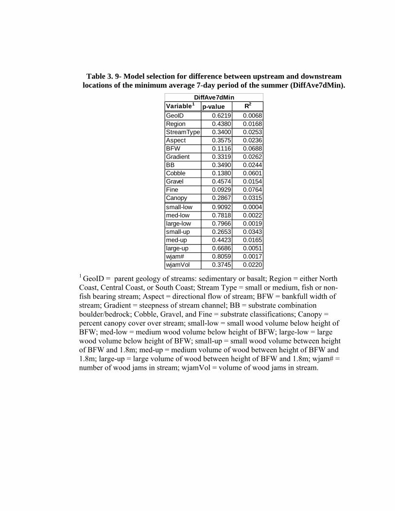
Table 3. 9- Model selection for difference between upstream and downstream locations of the minimum average 7-day period of the summer (DiffAve7dMin).
Variable1 p-value R2
GeoID 0.6219 0.0068Region 0.4380 0.0168StreamType 0.3400 0.0253Aspect 0.3575 0.0236BFW 0.1116 0.0688Gradient 0.3319 0.0262BB 0.3490 0.0244Cobble 0.1380 0.0601Gravel 0.4574 0.0154Fine 0.0929 0.0764Canopy 0.2867 0.0315small-low 0.9092 0.0004med-low 0.7818 0.0022large-low 0.7966 0.0019small-up 0.2653 0.0343med-up 0.4423 0.0165large-up 0.6686 0.0051wjam# 0.8059 0.0017wjamVol 0.3745 0.0220
DiffAve7dMin
1 GeoID = parent geology of streams: sedimentary or basalt; Region = either North Coast, Central Coast, or South Coast; Stream Type = small or medium, fish or non-fish bearing stream; Aspect = directional flow of stream; BFW = bankfull width of stream; Gradient = steepness of stream channel; BB = substrate combination boulder/bedrock; Cobble, Gravel, and Fine = substrate classifications; Canopy = percent canopy cover over stream; small-low = small wood volume below height of BFW; med-low = medium wood volume below height of BFW; large-low = large wood volume below height of BFW; small-up = small wood volume between height of BFW and 1.8m; med-up = medium volume of wood between height of BFW and 1.8m; large-up = large volume of wood between height of BFW and 1.8m; wjam# = number of wood jams in stream; wjamVol = volume of wood jams in stream.

Table 3.10- Model selection for difference between upstream and downstream locations of the maximum 7-day diurnal fluctuation (DiffMax7dDiFlux).
Variable1 p-value R2
GeoID 0.5401 0.0105Region 0.1412 0.0591StreamType 0.1868 0.0479Aspect 0.8561 0.0009BFW 0.5845 0.0084Gradient 0.5890 0.0082BB 0.7380 0.0031Cobble 0.6030 0.0076Gravel 0.3205 0.0274Fine 0.3282 0.0266Canopy 0.0167 0.1491small-low 0.7635 0.0025med-low 0.7203 0.0036large-low 0.5541 0.0098small-up 0.2390 0.0383med-up 0.4490 0.0160large-up 0.9424 0.0001wjam# 0.7185 0.0037wjamVol 0.4745 0.0143
DiffMax7dDiFlux
1 GeoID = parent geology of streams: sedimentary or basalt; Region = either North Coast, Central Coast, or South Coast; Stream Type = small or medium, fish or non-fish bearing stream; Aspect = directional flow of stream; BFW = bankfull width of stream; Gradient = steepness of stream channel; BB = substrate combination boulder/bedrock; Cobble, Gravel, and Fine = substrate classifications; Canopy = percent canopy cover over stream; small-low = small wood volume below height of BFW; med-low = medium wood volume below height of BFW; large-low = large wood volume below height of BFW; small-up = small wood volume between height of BFW and 1.8m; med-up = medium volume of wood between height of BFW and 1.8m; large-up = large volume of wood between height of BFW and 1.8m; wjam# = number of wood jams in stream; wjamVol = volume of wood jams in stream.
3.2 Stream Temperature Patterns of Tracer Test Streams Stream temperatures were graphed for 2002 and 2003 on the four streams
selected for additional study of streamwater residence time to determine effects of
stream temperature changes between years on residence time (Figure 3. 22 and Figure
3. 23). Two streams (Toad Creek, stream #12 and Beeches Creek, stream #20)
showed a downstream cooling pattern in 2002 and 2003 with a high degree of
variability along the stream reach. Ice Box (stream #9) warmed in a downstream
direction with the middle reach significantly warmer. Nettle Meyer Creek (stream #6)
warmed in a simple downstream direction.
3.2.1 Beeches Creek (Stream #20)
The Downstream tracer test on Beeches Creek was conducted on July 29, 2003
(Table 3.11). Background conductivity was 0.057 mS/cm. The test began at 8:36
when 5000g of salt were placed 60 m above the bottom of the Downstream Reach.
Conductivity decreased to within 15% of background conductivity and the test was
terminated at 17:07 on July 29th at a conductivity of 0.067 mS/cm. Observed
residence time for this reach was 7.5 hours. Calculated residence time was 9 hours.
Stream temperature in this reach increased in both 2002 and 2003.
The test on the Treatment Reach of Beeches Creek began at 13:35 on August
3, 2003 when 5000g of salt were placed 60 m above the bottom of the Treatment
Reach (Table 3.11). Background conductivity was 0.055 mS/cm. The test continued
until 7:36 on August 4, 2003 when the tail of the tracer test decreased to within 5% of
background concentrations (0.061 mS/cm). Observed residence time on this reach
was 17 hours and calculated residence time was 18 hours. Stream temperature in this
reach increased in 2002 and decreased in 2003.
The test on the Control Reach of Beeches Creek began at 6:46 on July 31,
2003 when 4000g of salt were added 60 m above the bottom of the Control Reach
(Table 3.11). Background conductivity was 0.044 mS/cm. Tail concentrations only
decreased to within 31% of initial conductivity (0.065 mS/cm). Observed residence

time on this reach was 8.5 hours and calculated residence time was 12 hours. Stream
temperature in this reach decreased in both 2002 and 2003.
1 2 3 412
13
14
15
16
17
18
Temperature Probe
Max
7d (°
C)
Toad (#12)
Beeches (#20)
Nettle Meyer (#6)
Ice Box (#9)
Figure 3. 22- 2002 Max7d temperatures for 4 streams chosen
for tracer tests.
1 2 3 412
13
14
15
16
17
18
Temperature Probe
Max
7d (°
C)
Toad (#12)
Beeches (#20)
Nettle Meyer (#6)
Ice Box (#9)
Figure 3. 23- 2003 Max7d temperatures for 4 streams chosen
for tracer tests.
3.2.2 Nettle Meyer (Stream #6)
The test began on the Downstream Reach of Nettle Meyer Creek on August 4,
2003 at 13:48 when 6000g of salt were placed 60 m above the bottom of the study site
(Table 3.11). Initial background conductivity was 0.055 mS/cm. At approximately
15:45 the test was considered complete when conductivity at the probe returned to
within 10% of initial conductivity at 0.061 mS/cm, but the test was allowed to
continue until18:40. Observed and estimated residence time for this reach was 4.5
hours. Stream temperature increased in this reach in 2002 and 2003.
The tracer test for the Treatment Reach of Nettle Meyer Creek began at 19:03
on August 4, 2003 when 3000g of salt were placed 60 m above the bottom of the
Treatment Reach (Table 3.11). Background conductivity was 0.056 mS/cm. The test
was complete at 21:20 when concentrations reached 0.062 mS/cm but was not
terminated until 1:37am on August 5th. Observed and estimated residence time for this
reach was 6 hours. Stream temperature remained approximately the same in this reach
in 2002 and 2003.
The tracer test for the Control Reach of Nettle Meyer Creek began at 2:11 am
on August 5th 2003 when 3000g of salt were placed 60 m below the top of the study
site (Table 3.11). Background conductivity was 0.057 mS/cm. The test was
completed 8:11 on August 5, 2003. Observed and estimated residence times were 4.5
hours for this reach. Stream temperature increased in 2002 and was not available for
2003.
3.2.3 Ice Box (Stream #9)
The tracer test for the Treatment Reach of Ice Box Creek began at 12:08 on
August 5 2003 with the addition of 6000g of salt (Table 3.11). Initial conductivity
was 0.036 mS/cm. The test was terminated slightly early at only 0.41 mS/cm (within
11 percent of initial conductivity) at 14:27 on August 6 2003. Observed residence
time was 24 hours and estimated residence time was 27 hours for this reach. Stream
temperature decreased in 2002 and was not available in 2003.
The tracer test for the Control Reach of Ice Box Creek began at 8:28 on August
21 2003, when 5000g of salt were placed 60 m below the top of the study site (Table
3.11). Background conductivity was 0.037 mS/cm. The test was terminated early at
9:16 on August 22 2003 within only 14% of initial conductivity. Observed residence
time for this reach was 22 hours and estimated residence time was 25 hours. Stream
temperature increased substantially in this reach in 2002 and 2003.
3.2.4 Toad Creek (Stream #12)
The tracer test for the Downstream Reach of Toad Creek began on August 28
2003 at 8:55 when 7000g of salt were placed 60 m above the bottom of the reach
(Table 3.11). Background conductivity was 0.047 mS/cm. The test was terminated at
14:12 of August 29, 2003 when conductivity was 0.049 mS/cm. Observed residence
time was 28 hours and estimated residence time was 29 hours. Stream temperature
increased in this reach in 2002 and 2003.
The tracer test for the Treatment Reach of Toad Creek began on August 18,
2003 at 10:02 when 6000g of salt were placed 60 m above bottom of the Treatment
Reach (Table 3.11). Initial background concentrations were 0.047 mS/cm. The test
was terminated at 19:10 on the same day. After nine hours, no trace of salt appeared
at the conductivity probe. Stream temperature decreased substantially in this reach in
2002 and 2003.
The tracer test for the Control Reach of Toad Creek began at 20:11 on the
August 18, 2003 when 4000g of salt were placed 60 m below the top of the study site
(Table 3.11). Background conductivity was 0.041 mS/cm. The test was terminated
early at only 18% of background conductivity at 6:03 on August 21 2003. After
almost 3 ½ days, this was considered sufficient for the purpose of this study.
Observed residence time was 54 hours and estimated residence time was 61 hours.

Stream temperature in this reach remained approximately the same in 2002 and
increased in 2003.
Table 3. 11- Results of tracer tests on four streams in the Oregon Coast Range.
Site ReachAmount
of SaltStart Time End Time
Observed Residence
Time
Calculated Residence
TimeBeeches Downstream 5000g 7/29/03 8:36 7/29/03 17:07 7.5 9
Treatment 5000g 8/3/03 13:37 8/4/03 7:30 17 18Control 4000g 7/31/03 6:46 7/31/03 16:26 8.5 12
Nettle Meyer Downstream 6000g 8/4/03 13:48 8/4/03 18:40 4.5 4.5Treatment 3000g 8/4/03 19:03 8/5/03 1:37 6 6Control 3000g 8/5/03 2:11 8/5/03 8:11 4.5 4.5
Ice Box Treatment 6000g 8/5/03 12:08 8/6/03 14:27 24 27Control 5000g 8/21/03 8:28 8/22/03 9:16 22 25
Toad Creek Downstream 7000g 8/28/03 8:55 8/29/03 14:12 28 29Treatment 6000g 8/18/03 10:02 8/18/03 19:10 * *Control 4000g 8/18/03 20:11 8/21/03 6:03 54 61
*Background conductivity on this reach of Toad Creek did not display any signs of increasing 9 hours after the tracer test began. A significant portion of the flow from
this reach was subsurface.
3.2.5 Relationship between residence time and temperature change
No direct relationship was found for changes between upstream and
downstream locations of streamwater temperature and residence time (R2 = 0.0059)
(Figure 3.24). Reaches with short residence times displayed both cooling and heating
temperature patterns downstream. Reaches with longer residence times also did not
exhibit a distinct temperature trend.
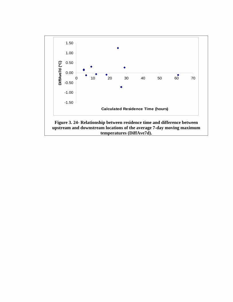
-1.50
-1.00
-0.50
0.00
0.50
1.00
1.50
0 10 20 30 40 50 60 70
Calculated Residence Time (hours)
Diff
Ave7
d (°
C)
Figure 3. 24- Relationship between residence time and difference between
upstream and downstream locations of the average 7-day moving maximum temperatures (DiffAve7d).

Chapter IV
Discussion
4.1 Stream Temperature Characteristics
4.1.1 General and Longitudinal Variation of Stream and Riparian Characteristics The three separate reaches designated for each stream in this study were
chosen based on future logging plans as opposed to the natural layout of the stream
channel. For example, one whole “stream” in this study could be concentrated entirely
in the headwaters of a basin and another “stream” entirely in the valley bottom,
depending on where logging was planned. Therefore, each stream could still have its
respective 3-reach design and be within the classification confines of this study, but
could be in contrasting geomorphological settings. This potential source of variation
among the 38 study streams should be considered in evaluation of spatial variability
among stream channel and riparian characteristics. Despite this limitation, data from
the study streams help to characterize the variability within small headwater streams
of the Oregon Coast Range. Much of the variability among stream and riparian
characteristics is due to the study design, but natural heterogeneity of streams in the
Coast Range is also apparent within and among the streams. Zwieniecki and Newton
(1999) also found a wide range of stream characteristics on 14 small streams in
western Oregon. Sullivan and Adams (1989) studied 24 streams in Oregon and
Washington and found a wide range of characteristics as well.
Average riparian canopy cover of 92% in this study represents a well-shaded
forested headwater stream in the Oregon Coast Range (Beschta et al. 1987). Other
studies (Levno and Rothacher 1967, Beschta and Taylor 1988, Jackson et al. 2001) of
canopy cover prior to logging in the Pacific Northwest have reported similar canopy
conditions as observed in this study. Streams used in the current study are also similar

to those described by Brown and Krygier (1970) in the Alsea watershed in the Oregon
Coast Range.
Small wood was the most abundant size classification occurring in this study,
whereas large wood was the scarcest, agreeing with observations reported by Keim et
al. (2000) that small wood is most abundant and most mobile in coastal Oregon
streams. Jackson et al. (2001) characterized large wood before and after logging in the
Coast Range of Washington and also found a dominance of small wood.
The general lack of longitudinal substrate patterns was most likely a product of
study design limitations. Contrary to other studies of longitudinal gradients (Vannote
et al. 1980, Tabacchi et al. 1998), we did not find predictable longitudinal patterns of
substrate composition. For example, in this study fine substrate slightly decreased
downstream, while percent bedrock and boulder slightly increased. This observation
contrasts with ideas presented in the River Continuum Concept (Vannote et al. 1980)
that suggest presence of more bedrock and boulder upstream and more fine substrate
in downstream reaches with decreasing gradient. The absence of strong longitudinal
substrate patterns in this study may be because our study design only spanned 1-2
stream orders, whereas the River Continuum Concept spans approximately seven
stream orders (Vannote et al. 1980).
Tabacchi et al. (1998) also describe predictable longitudinal patterns of stream
and riparian characteristics related to location within the riparian corridor. Our
observations of decreasing percent canopy cover, increasing bankfull width, and
decreasing percent gradient of the channel in downstream reaches indicated a
flattening and opening of the stream basins. These results concur with observations of
Lewis et al. (1999) for streams in northern California, who reported that as stream
channels become flatter and valleys widen, percent shade over the streambed
decreases, indicating an opening of the valley floor.
4.1.2 Streamwater Temperature
Stream temperature differences between 2002 and 2003 on 21 of the same
streams can be attributed to a difference in climatic conditions between the two years.
Stream temperature variation due to climatic variability has been found to be between
2 to 4°C in a variety of locations and thus a climatic difference of approximately 1°C
was not considered an unexpected difference for this study (Beschta et al. 1987).
Average daily maximum temperature for the summer (June-August) of 2002 for the
north Oregon Coast was 26.9 ºC and for 2003 was 28.1ºC (NOAA, National Climatic
Data Center for McMinnville, Oregon). Therefore, 2003 was warmer overall and this
could explain the stream temperature variability between the two summers.
All streams in this study did not follow simple downstream warming patterns.
Poole and Berman (2001) cite similar inconsistencies in stream temperature patterns
and Ebersole et al. (2003) found heterogeneous longitudinal patterns of summer
stream temperature in northeastern Oregon. In contrast, Brown (1970), Zwieniecki
and Newton (1999), and Lewis et al. (1999) found small streams to have predictable
patterns of warming in a downstream direction under full canopy cover. Possible
explanations for cooler middle or lower reaches as observed in some streams in the
current study include entrance of cool tributaries and influx of groundwater (Beschta
et al. 1987, Ebersole et al. 2000).
Currently, the Oregon Department of Forestry expresses temperature responses
as a 7-day moving mean of daily maximum temperatures (7dMMDMax). This study
found a range of 11.4 to 16.8 °C among the 38 streams using the Max7d measurement
(the warmest 7-day period of the summer). The current upper limit for water quality
of 7-day temperatures for the Oregon Coast Range is 16 °C and three of these 38
streams have natural temperature regimes before harvesting above this level. This
demonstrates the inherent natural variability in stream temperature in this area and the
importance of defining the pre-disturbance temperature regime of a stream for
assessing management effects. In addition, the average of the weekly high
temperatures for the summer (Ave7d) correlated closest to stream and riparian
variables measured in this study. This suggests that a response variable such as
average weekly high temperature might be a more sensitive indicator in analyzing
effects of riparian management on stream temperature.
4.1.3 Relationship between Stream and Riparian Variables and Stream Temperature Stream temperature was only weakly correlated to variables derived from
information gathered from GIS sources. A weak relationship between high stream
temperatures and stream aspect was evident with southern and southwestern facing
streams, particularly for peak temperatures later in the summer. Solar radiation will
likely be most influential in the Oregon Coast Range in the late afternoon and
therefore, south and south-western facing streams should have later summertime peaks
as the late afternoons become increasingly warmer. In northern California, Lewis et
al. (1999), found streams flowing N-S had a slightly higher average daily maximum
temperature than streams flowing E-W. However, this characteristic did not show any
significant association with stream temperature and is not considered significant for
coastal headwater streams in this study. Stream orientation was also derived from GIS
and therefore may not display the most accurate aspect of the whole stream.
The model selection process clearly demonstrates that stream temperature is
significantly correlated with selected stream channel and riparian variables that were
measured at each site. Canopy cover, either alone or with another variable, was the
most consistent significant variable in the best-fit models, accounting for significant
variation in five out of the eight temperature response variables. This result concurs
with studies by Brown (1970), Brown (1988), Beschta et al. (1987) Lewis et al.
(1999), and Zwieniecki and Newton (1999) reporting the importance of shade for
maintaining stream temperature. Conversely, Hewlett and Fortson (1982) determined
groundwater input to be the primary driver of stream temperature in small streams in
the southeastern U.S. Sullivan and Adams (1989) also questioned the concept of
shade as the sole driver of stream temperature arguing that air temperature, stream
depth, and groundwater contributions also play an important role in temperature
patterns.
The three temperature responses based on difference in maximum temperatures
between upstream and downstream locations (DiffMax7d, DiffMaxDailyMax,
DiffAve7dMax) all included canopy cover as an important explanatory variable in the
model. Solar radiation has been shown to be a key driver of midday high temperatures
(Beschta and Taylor 1988, Brown 1988, Sinokrot and Stefan 1993) and this is
displayed in the incorporation of canopy cover in all three models.
The model that accounts for the most variability in this study negatively
correlates the average weekly high stream temperature for the summer
(DiffAve7dMax) to canopy cover and volume of wood jams in the stream. Wood jam
volume is important because of the possibility of increasing the residence time of
water in a section of the channel by forming pools (Stack and Beschta 1989) and
increasing localized shade in an area that may otherwise be exposed (Heifetz et al.
1986). Jackson et al. (2001) suggest that accumulations of large wood aid in forming
and maintaining riffle-pool morphology in small streams. It should be noted that
while this model accounts for the most variability in maximum stream temperature,
the cross-check with AIC model selection favored the model with simply canopy
cover. This model based on canopy cover and volume of wood jams represents 51%
of the variability in average weekly high temperature, demonstrating that there is half
of the variability in the temperature response still unexplained by measured stream and
riparian characteristics. This suggests that stream temperature may be more strongly
influenced by characteristics of the stream channel or riparian area that were not
measured in this study. For example, stream temperature has been suggested to be
closely correlated to air temperature in a variety of studies (Holtby 1988, Sullivan and
Adams 1989). Air temperature in each riparian corridor was not measured in this
study. Conversely, it is possible that characteristics of the streams chosen for this
study did not provide an adequate range of conditions among streams to clearly
decipher relationships with stream temperature. Despite these shortcomings in
explaining stream temperature patterns, there is enough variability in average weekly
high temperatures explained by canopy cover and wood jam volume to provide a
solid foundation from which to assess changes in canopy and wood jam volume
resulting from impending harvest practices and subsequent temperature responses.
Wood jam volume, region, and bankfull width are significant explanatory
variables in the model with the absolute maximum 7-day period averaged over the
three bottommost probes on each stream (Max7d). Canopy cover was not a significant
variable in this model likely because this temperature response is an average from
probes along a stream and not a temperature change between upstream and
downstream conditions. By averaging the temperature responses along a stream
channel, any significant change in temperature between upstream and downstream
becomes muted and measured stream and riparian characteristics will have a different
influence on this response variable due mainly to the method of derivation.
Minimum temperature variables were less consistently correlated to one
dominant explanatory variable than maximum temperature variables. The coldest 7-
day period of the summer (DiffMin7dMin) was most strongly correlated to percent
fine substrate, and the coldest day of the summer (DiffMinDailyMin) was correlated
with geology and canopy cover. These results demonstrate that minimum
temperatures are closely correlated to a substrate characteristic. Supporting these
findings are results from Ebersole et al. (2003) who describes that cool water in small
streams is associated with substrate characteristics and localized conditions. Although
not found in this study, substrate characteristics are often indicators of other stream
characteristics such as gradient and discharge (Vannote et al. 1980, Tabacchi et al.
1998) and it may be that substrate is significant in these models as an indicator for
other unmeasured characteristics. In this study, the coldest periods occurred during
the beginning of the summer or late spring when air temperatures were still fairly cool
in the Coast Range and sun angles had not reached maximum. Therefore, cool
temperatures may be responding to conductive heat exchange with the substrate,
whereby the slightly warmer stream water is losing heat to the still seasonally cool
substrate (Brown 1988). This hypothesis corresponds to the findings of Sinokrat and
Stefan (1993) who found that conduction between shallow, small streams and the
streambed should be considered in heat budget estimates. Minimum temperatures
usually occur in the early morning. Here, canopy cover keeps air temperatures near
the stream cool during the day, not allowing the temperature of the water to heat
significantly with increasing temperatures of late spring/early summer. This agrees
with findings of Sullivan and Adams (1989) who reported that protection from direct
solar radiation keeps stream temperatures in small streams near groundwater
temperatures.
In contrast, average minimum temperatures of the summer (DiffAve7dMin)
were not correlated to measured channel or riparian variables. Minimum stream
temperatures vary greatly (4.3-16.8 °C in 2002 and 2003) over the summer as air and
water temperatures increase. Therefore, an average of these temperatures does not
accurately measure any one representative minimum value and is subsequently not
significantly correlated to any one stream or riparian characteristic.
The temperature flux response variable (DiffMax7dDiFlux) was weakly
correlated to canopy cover. As percent canopy cover increases, the maximum diurnal
flux approaches zero. Therefore, in areas with less canopy cover and more exposure
to solar radiation, there is likely greater difference between daily temperature
extremes. Beschta et al. (1987) found that diurnal variations increased with removal
of shade, thus concurring with the findings from this study.
4.2 Tracer Experiments
Observations of residence time and change in temperature within the
corresponding reach were examined to explore the hypothesis that streams with
cooling reaches had longer residence times. If results had supported our hypothesis,
negative temperature responses (the difference in temperature from upstream to
downstream location) would correlate to longer residence times. Long residence times
suggest a reach of the stream with interactions, such as exchange with the hyporheic
zone, water eddying behind or under log jams, and complex exchanges with
subsurface water resulting in potential cooling mechanisms. Conversely, long
residence times can also indicate water remaining in slow moving pools or very low
flows resulting in potential heating mechanisms as streamwater is subjected to more
solar radiation and convection. Harvey and Bencala (1993) found that complex
streambed topography increased interaction between surface water and groundwater
and thus potentially extended residence time of water in the stream. A warming reach
was hypothesized to either (1) be a losing reach, with decreasing flow along a
specified length (Constantz et al. 1994) or (2) have a significant portion of the water
simply remaining in the stream and susceptible to warming from solar radiation
(Beschta and Taylor 1988, Poole and Berman 2001).
Upon analysis, it is clear that observed residence time and temperature patterns
of some streams are consistent with our original hypothesis of longer residence time in
cooling reaches and shorter residence times in warming streams. For example, Nettle
Meyer Creek had the shortest residence times and was the only stream that warmed in
a downstream direction, concurring with stream temperature patterns reported by
Brown (1970) and Zwieniecki and Newton (1999). This suggests that water is not
being retained in the stream for long periods of time and it can be deduced that there is
probably limited exchange of water with the hyporheic zone. Therefore this stream
conforms to the simple temperature models of increasing energy inputs and rising
temperature downstream (Brown 1970).
Observations at Toad Creek also supported our hypothesis of cooling reaches
responding to longer residence times. It is interesting to note that in both 2002 and
2003, the middle reach of Toad Creek decreased between 2 and 5 °C. In the tracer test
on this reach no trace of the added salt appeared after 9 hours of observation. There
was approximately 30 m without surface flow at the time of tracer tests in this portion
of the channel, indicating that the stream flowed below the channel and reappeared
with lower temperature downstream. There is a strong potential for this portion of the
channel to be interacting with the hyporheic zone (White 1993, Malard et al. 2002),
although to make that assumption is beyond the scope of this study and is merely
speculative. Malard et al. (2002) suggested that continued subsurface flow under a
series of connected riffles in Sycamore Creek, Arizona decreased surface water
temperatures by as much as 4°C, concurring with the findings from this study reach.
The control reach of Toad Creek also had a long residence time. Much of this
reach is characterized by bedrock and was expected to have a short residence time
because groundwater/surface water exchange is usually restricted in bedrock-
dominated streams (Hendricks and White 1991, Malard et al. 2002). There is a
significant waterfall partway up this reach and it is possible that water was retained in
an eddy near the waterfall. In 2002 this portion of the stream did not change
temperature and in 2003 it warmed by 1.5°C. Therefore, streamwater residence time
in this portion of the stream may be primarily influenced by the complexity (wood
jams and eddies) in and around the waterfall. This concurs with Harvey and Bencala’s
(1993) assessment of complex channel morphology influencing streamwater
interactions. This hypothesis also is supported by Malard et al. (2002), who suggest
that localized barriers to flow initiate subsurface flow into the hyporheic zone
subsequently increasing streamwater residence time, although this does not explain
temperature responses seen in this reach.
It is also possible that the dominance of bedrock in the Control Reach of Toad
Creek contributed to conduction of warmer temperatures from the bedrock to the
stream water. Johnson and Jones (2000) reported conduction from substrate to be an
important contributor to increased stream temperatures after logging in western
Oregon. Although this is a forested reach, the warm stream temperature may indicate
that solar radiation and conduction are both mechanisms of stream heating in this case.
The downstream portion of this stream had a shorter residence time than the other two
reaches and warmed in both 2002 and 2003, although two significant tributaries
entered the stream just above the point where the tracer test was initiated. Brown
(1988) suggested that changes in temperature by inflowing tributaries are dependent
upon discharge and therefore small tributaries will not impact the temperature of the
main stream significantly. Here, it must be assumed that the tributaries were not
significantly cooler than the main stem of the stream and there was not a large portion
of groundwater upwelling.
For the stream Ice Box, residence times of the two reaches were of similar
duration (estimated at 25 and 27 hours) even though temperature regimes and stream
characteristics are much different between these reaches. The control reach was flat
and characterized by mostly gravel, very slow moving pools, and less canopy cover
allowing for sunlight to hit the surface of the stream. This suggests that water is
interacting with this gravel dominated stream, providing tortuous pathways and
residing in the long, shallow, slow moving pools. Water moved very slowly in this
portion of the stream and with the increased exposure to sunlight had a high potential
to warm in this reach (Beschta and Taylor 1988, Sinokrot and Stefan 1993). In
between these two reaches was a culvert that significantly altered the stream channel
characteristics and therefore the treatment reach of this stream was different than the
control reach. This reach was characterized by a high amount of canopy cover, a steep
gradient, and an abundance of large wood and boulders. It is likely that this stream
responded to the increased complexity of the channel and was detained behind large
wood and in cool, deep pools, thus cooling downstream. A number of studies have
shown that increasing complexity of geomorphological characteristics in the stream
channel increase the likelihood of subsurface flow (Malard et al. 2002, Harvey and
Bencala 1993, White 1993). In addition, Findlay (1995) also found that variability in
residence times can be attributed to complexities such as morphology of the channel
and substrate characteristics. In this stream, varying stream characteristics as a
possible result of the culvert can influence stream temperature.
Beeches Creek also did not display expected residence time- stream
temperature relations. This was a very complex stream with many waterfalls, steep
gradients, wood jams, and mixed substrate. There were no significant differences in
the complexity of this stream among reaches, and therefore it is difficult to explain
differences in residence times among reaches. For example the longest residence time
on this stream (18 hours) was the middle reach, which warmed in 2002 and cooled in
2003, whereas the control reach had a 12-hour residence time and cooled in 2002 and
2003, and the downstream reach warmed in both years and had a residence time of 9
hours.
These findings are inconclusive regarding relationships between residence time
and longitudinal patterns of streamwater temperature. Whereas some streams did have
long residence times, these were not always cooling reaches as opposed to findings by
Malard et al. (2002) who described that subsurface exchange decreased stream
temperature. Therefore, there may be other processes occurring in these streams that
contribute to stream temperature patterns. For example, in warming streams with long
residence times, water may be retained in slow moving pools. In this case, with an
increasing surface area exposed to solar radiation, warming will occur (Beschta and
Taylor 1988). In contrast, cooling streams with short residence times may have a
reach receiving groundwater upwelling or a tributary contributing cooler water in the
middle of the reach (Ebersole et al. 2003). In addition, the 152 m reach for these
tracer tests may have been too long to get an accurate estimate of stream processes
occurring at more localized scales. Other tracer studies have concentrated on
significantly shorter reaches of streams, attempting to quantify local surface
water/groundwater exchanges (Constantz et al. 1994, Evans and Petts 1997, White et
al. 1987).

Chapter V
Conclusions and Management Implications
This study provides additional insight into the complexity of processes
influencing stream temperature in small headwater stream systems of the Oregon
Coast Range with implications for management. Traditionally in forest management,
shade is provided by maintaining riparian buffer zones to protect streams from adverse
impacts of harvesting operations on temperature. As noted in the results of this study,
canopy cover is a driving factor influencing summertime stream temperature patterns
and energy inputs from direct solar radiation are usually the dominant factor in energy
budget calculations concerning stream temperature. However, the inherent complexity
in small streams observed in this study indicates that other processes are important as
well and should not be discarded in considerations of forest management effects on
stream temperature.
Other variables besides canopy cover can play an important role in the
temperature dynamics of small streams. Volume of wood jams in a stream, substrate
composition, parent geology, and width of the stream channel are additional variables
that aid in explaining summertime temperature patterns in the stream and disregarding
these variables may decrease the amount of temperature variability explained by
stream characteristics.
In stream temperature studies undertaken by the Oregon Department of
Forestry in the Coast Range, the maximum 7-day moving average (Max7d) and the
maximum daily temperature (MaxDailyMax) of the summer are the conventional
temperature metrics. However, for the streams in this study the average of the weekly
high temperatures for the summer (Ave7dMax) correlated closest to stream and
riparian variables measured. Therefore, it may be more appropriate to analyze a range
of high temperatures as opposed to only the hottest week of the summer when
assessing effectiveness of riparian management practices.
This study also demonstrates the high degree of variability among summertime
stream temperature patterns in headwater streams of the Oregon Coast Range. These
natural patterns of stream temperature are an important consideration for background
characterization of water quality prior to assessment of effects of forest management
practices. Once these areas have been harvested and stream temperature responses are
examined, it will be imperative to be aware of the widely varying longitudinal patterns
of stream temperature that existed prior to disturbance. The high degree of variability
observed among streams prior to harvesting also suggests that it may be difficult to
extrapolate harvesting effects beyond streams in which they are measured.
In the experiments to determine the residence time of water, results did not
consistently support expectations of cooling temperatures with longer residence times.
Upon further consideration, residence time alone should not be used to predict the
temperature change of water in a stream. A stream that cools in a downstream
direction may not necessarily be caused by long residence time but more a function of
stream channel characteristics such as inflowing tributaries, wood jams, gradient,
exposure to sunlight, and groundwater influx. In general, it is probable that cooling
reaches of streams have complex processes taking place besides simply water flowing
down the stream.
Even in the height of summer, at a time when flows are approaching their
annual lows, and solar radiation and air temperatures are maximum, it is still possible
for streamwater to cool downstream. This indicates that other processes besides solar
radiation and low flows are contributing to changes in stream temperature. In this
study, results did not explicitly demonstrate that cooling reaches had long residence
times. This indicates that exchange with the hyporheic zone may not be the only
factor or the driving factor contributing to cooling reaches. Groundwater upwelling
may be a more prevalent phenomenon in small headwater streams in the Oregon Coast
Range. Therefore, we cannot conclude that cooling reaches of streams are entirely
attributed to increased residence times but may be due to other stream processes.
Temperature regimes of small streams in the Oregon Coast Range are
primarily correlated with canopy cover over the stream, but patterns within these

stream systems are longitudinally variable and temperature responses to management
practices will likely not be uniform across this region. As such, assessment of local
conditions within each stream and the adjacent riparian zones is an important
consideration in understanding the dynamics of streamwater temperature.
References
Adams, T. N., and K. Sullivan. 1989. The Physics of Forest Stream Heating: A Simple Model. Weyerhaeuser Research Project. Project No. 044-5002/89/1.
Alexander, M. D., and D. Caissie. 2003. Variability and Comparison of Hyporheic Water Temperatures and Seepage Fluxes in a Small Atlantic Salmon Stream. Groundwater 41: 72-82.
Beschta, R. L. 1997. Riparian Shade and Stream Temperature: An Alternative Perspective. Rangelands 19: 25-28.
Beschta, R. L., R. E. Bilby, G. W. Brown, L. B. Holtby, and T. D. Hofstra. 1987. Chapter Six: Stream Temperature and Aquatic Habitat: Fisheries and Forestry Interactions. Streamside Management: Forestry and Fishery Interactions: 191-232.
Beschta, R. L., and R. L. Taylor. 1988. Stream Temperature Increases and Land Use in a Forested Oregon Watershed. Water Resources Bulletin 24: 19-25.
Bond, B. J., J. A. Jones, G. Moore, N. Phillips, D. Post, and J. J. McDonnell. 2002. The zone of vegetation influence on baseflow revealed by diel patterns of streamflow and vegetation water use in a headwater basin. Hydrological Processes 16: 1671-1677.
Boulton, A. J. 1998. The Functional Significance of the Hyporheic Zone in Streams and Rivers. Annual Review of Ecological Systems 29: 59-81.
Boulton, A. J., M. R. Scarsbrook, J. M. Quinn, and G. P. Burrell. 1997. Land-use effects on the hyporheic ecology of five small streams near Hamilton, New Zealand. New Zealand Journal of Marine and Freshwater Research 31: 609-622..
Brown, G. W. 1970. Predicting the effect of clearcutting on stream temperature. Journal of Soil and Water Conservation 25: 11-13.
Brown, G. W. 1988. Forest and Water Quality. OSU Bookstores, Inc., Memorial Union, Oregon State University, Corvallis, OR 97339
Brown, G. W., and J. T. Krygier. 1970. Effects of Clear-Cutting on Stream Temperature. Water Resources Research 6: 1133-1139.
Constantz, J., C. Thomas, and G. Zellweger. 1994. Influence of diurnal variations in stream temperature on streamflow loss and groundwater recharge. Water Resources Research 30: 3253-3264.
Constantz, J., C. L. Thomas, and G. Zellweger. 1994. Influence of diurnal variations in stream temperature on streamflow loss and groundwater recharge. Water Resources Research 30: 3253-3264.
Ebersole, J. L., Liss, William J., and Christopher A. Frissell. 2003. Cold Water Patches in Warm Streams: Physicochemical Characteristics and the Influence of Shading. Journal of the American Water Resources Association April: 355-368.
Evans, E. C., and G. E. Petts. 1997. Hyporheic temperature patterns within riffles. Hydrological Sciences 42: 199-213.
Findlay, S. 1995. Importance of surface-subsurface exchange in stream ecosystems: the hyporheic zone. Limnology and Oceanography 40: 159-164.
Harvey, J. W., and E. E. Bencala. 1993. The Effect of Streambed Topography on Surface-Subsurface Water Exchange in Mountain Catchments. Water Resources Research 29: 89-98.
Heifetz, J., M.L. Murphy, and K.V. Koski. 1986. Effects of logging on winter habitat of juvenile salmonids in Alaskan streams. North Am. J. Fish. Manage. 6:52-58.

Hendricks, S. P., and D. S. White. 1991. Physicochemical Patterns within a Hyporheic Zone of a Northern Michigan River, with Comments on Surface Water Patterns. Canadian Journal of Fisheries and Aquatic Sciences 48: 1645-1654.
Hewlett, J.D., and J.C. Fortson. 1982. Stream temperature under an inadequate buffer
strip in the southeast piedmont. Wat. Resources Bull. 18 (6): 983-988. Holtby, L. B. 1988. Effects of logging on stream temperatures in Carnation Creek,
British Columbia, and associated impacts on the coho salmon (Oncorhynchus kisutch). Can. J. Fish. Aquat. Sci. 45: 502-515.
Jackson, C.R., C.A. Sturm, and J.M. Ward. 2001. Timber Harvest Impacts on Small
Headwater Stream Channels in the Coast Ranges of Washington. Journal of the American Water Resources Association 37(6): 1533-1549.
Johnson, S. L., and J. A. Jones. 2000. Stream temperature responses to forest harvest
and debris flows in Western Cascades, Oregon. Canadian Journal of Fisheries and Aquatic Sciences 57: 30-39.
Johnson, S.L. in press. Factors influencing stream temperatures in small streams:
substrate effects and a shading experiment. Canadian Journal of Fisheries and Aquatic Sciences.
Jones, J. B., and R. M. Holmes. 1996. Surface-subsurface interactions in stream
ecosystes. Trends Ecol Evol 11: 239-242.
Keim, R.K., A.E. Skaugset, and D.S. Bateman. 2000. Dynamics of Coarse Woody
Debris Placed in Three Oregon Streams. Forest Science 46(1): 13-22. Kilpatrick, F.A. and E.D. Cobb. 1985. Measurement of discharge using tracers: U.S.
Geological Survey Techniques of Water-Resources Investigations, Book 3, Chapter A16, 52p.
Kilpatrick, F.A., and J.F. Wilson, Jr. 1982. Measurement of Time of Travel in Streams
by Dye Tracing: U.S. Geological Survey Techniques of Water-Resources Investigations, Book 3, Chapter A9, 27p.
Larson, L. L., and P. A. Larson. 2001. Influence of Thermal Gradients on the Rates of
Heating and Cooling of Streams. Journal of Soil and Water Conservation 56: 38-43.
Levno, A., and J. Rothacher. 1967. Increases in Maximum Stream Temperatures After Logging in Old-Growth Douglas-Fir Watersheds. USDA Forest Service Research Note PNW-65 PNW Forest and Range Experiment Station, Portland, Oregon.: 12 p.
Lewis, T. E., D. W. Lamphear, D. R. McCanne, A. S. Webb, J. P. Krieter, and W. D. Conroy. 1999. Executive Summary: Regional Assessment of Stream TemperaturesAcross Northern California and Their Relationship to
Various Landscape-Level and Site-Specific Attributes. Forest Science Project. Humboldt State University Foundation, Arcata, CA: 14 p.
Logan, Robert. 2002. Oregon’s Forest Protection Laws, An Illustrated Manual,
Oregon Forest Resources Institute, Portland, OR, 97204.
Malard, F., K. Tockner, M.-J. Dole-Olivier, and J. V. Ward. 2002. A landscape
perspective of surface-subsurface hydrological exchanges in river corridors. Freshwater Biology 47: 621-640.
Mitchell, S. 1999. A Simple Model for Estimating Mean Monthly Stream Temperatures After Riparian Canopy Removal. Environmental Management 24: 77-83.
Murray, G. L. D., R. L. Edmonds, and J. L. Marra. 2000. Influence of Partial Harvesting on Stream Temperatures, Chemistry, and Turbidity in Forests on the Western Olympic Peninsula, Washington. Northwest Science 74: 151-164.
Newton, M. 1998. Riparian Management for Timber, Fish, and Wildlife. 19th Forest Vegetation Management Conference: 14-19.
Newton, M., and M. Zwieniecki. 1996. Temperature and Streamflow Regulation by Streamside Cover. Oregon State University, Department of Forest Science.
Poole, G. C., and C. H. Berman. 2001. An Ecologcial Perspective on In-Stream Temperature: Natural Heat Dynamics and Mechanisms of Human-Caused Thermal Degradation. Environmental Management 27: 787-802.
Rutherford, J. C., S. Blackett, C. Blackett, L. Saito, and R. J. Davies-Colley. 1997. Predicting the effects of shade on water temperature in small streams. New Zealand Journal of Marine and Freshwater Research 31: 707-721.
Shepherd, Bruce G., Gordon F. Hartman, and William J. Wilson. 1986. Relationships between stream and intragravel temperatures in coastal drainages, and some implications for fisheries workers. Canadian Journal of Fisheries and Aquatic Sciences. 43: 1818-1822.
Sinokrot, B. A., and H. G. Stefan. 1993. Stream Temperature Dynamics:
Measurements and Modeling. Water Resources Research 29:2299-2312.
Stack, W.R., and R.L. Beschta. 1989. Factors influencing pool morphology in Oregon
coastal streams. P. 401-411 in Proc. of a symp. On headwaters hydrology, Woessner, W.W. (ed.). Am. Water Resour. Assoc., Bethesda, MD.
Stringham, T. K., J. C. Buckhouse, and W. C. Krueger. 1998. Technical Note: Stream
Temperatures as related to subsurface waterflows originating from irrigation. Journal of Range Management 51: 88-90.
Sullivan, K., and T. N. Adams. 1989. The Physics of Stream Heating: 2) An analysis of temperature patterns in stream environments based on physical principles and field data. Weyerhaeuser Research Report Project No. 044-5002/89/2.
Tabacchi, E., D. L. Correll, R. Hauer, G. Pinay, A.-M. Planty-Tabacchi, and R. C. Wissmar. 1998. Development, maintenance and role of riparian vegetation in the river landscape. Freshwater Biology 40: 497-516.
Tanner, R. W. 2001. An evaluation of Temperature Prediction Models on Coastal Oregon and Western Cascade Streams. Master's thesis, Oregon State University, Department of Forestry.
Welty, J. J., T. Beechie, K. Sullivan, D. M. Hyink, R. E. Bilby, C. Andrus, and G. Pess.
2002. Riparian aquatic interaction simulator (RAIS): a model of riparian forest dynamics for the generation of large woody debris and shade. Forest Ecology and Management 162: 299-318.
White, D. S. 1993. Perspectives on defining and delineating hyporheic zones. Journal of the North American Benthological Society 12: 61-69.
White, D. S., C. H. Elzinga, and S. P. Hendricks. 1987. Temperature patterns within the hyporheic zone of a northern Michigan River. Journal of the North American Benthological Society 6: 85-91.
Zwieniecki, M. A., and M. Newton. 1999. Influence of streamside cover and stream features on temperature trends in forested streams of western Oregon. Western Journal of Applied Forestry 14: 106-113.

Appendix A
Reach Lengths
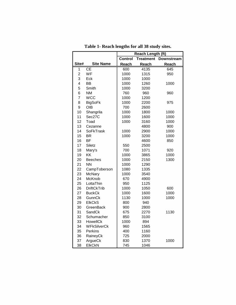
Table 1- Reach lengths for all 38 study sites.
Site# Site NameControl Reach
Treatment Reach
Downstream Reach
1 CE 600 4135 6452 WF 1000 1315 9503 Eck 1000 10004 BB 1000 1260 10005 Smith 1000 32006 NM 760 960 9607 WCC 1000 12008 BigSoFk 1000 2200 9759 OIB 700 260010 Shangrila 1000 1800 100011 Sec27C 1000 1600 100012 Toad 1000 3160 100013 Cezanne 4800 90014 SoFkTrask 1000 2900 100015 BR 1000 3200 100016 BF 4600 85017 Siletz 550 250018 Mary's 700 1071 92019 KK 1000 3865 100020 Beeches 1000 2150 130021 NN 1000 129022 CampToberson 1080 133523 McNary 1000 354024 McKnob 670 490025 LottaThin 950 112526 DriftCkTrib 1000 1050 60027 BuckCk 1000 1600 100028 GunnCk 1130 1000 100029 ElkCkS 800 94030 GreenBack 900 280031 SandCk 675 2270 113032 Schumacher 850 310033 HowellCk 1000 89434 WFkSilverCk 960 156535 Perkins 400 116036 RaineyCk 725 200037 ArgueCk 830 1370 100038 ElkCkN 745 1046
Reach Length (ft)

Appendix B
Stream Temperature by Stream
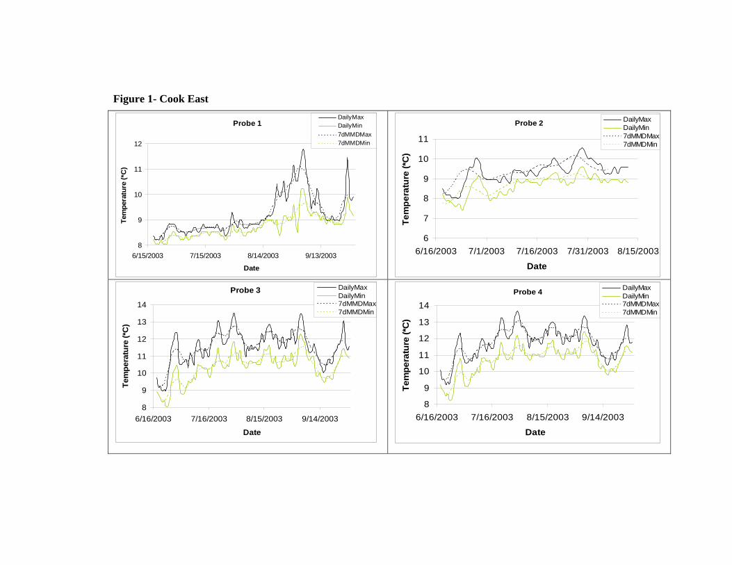
Figure 1- Cook East
Probe 1
8
9
10
11
12
6/15/2003 7/15/2003 8/14/2003 9/13/2003
Date
Tem
pera
ture
(*C
)DailyMaxDailyMin7dMMDMax7dMMDMin
Probe 2
6
7
8
9
10
11
6/16/2003 7/1/2003 7/16/2003 7/31/2003 8/15/2003
Date
Tem
pera
ture
(*C
)
DailyMaxDailyMin7dMMDMax7dMMDMin
Probe 3
8
9
10
11
12
13
14
6/16/2003 7/16/2003 8/15/2003 9/14/2003
Date
Tem
pera
ture
(*C
)
DailyMaxDailyMin7dMMDMax7dMMDMin
Probe 4
8
9
10
11
12
13
14
6/16/2003 7/16/2003 8/15/2003 9/14/2003
Date
Tem
pera
ture
(*C
)
DailyMaxDailyMin7dMMDMax7dMMDMin

Figure 2- Wolf’s Foot
Probe 1
8
9
10
11
12
13
14
6/16/2003 7/16/2003 8/15/2003 9/14/2003
Date
Tem
pera
ture
(*C
)
DailyMaxDailyMin7dMMDMax7dMMDMin
Probe 2
8
9
10
11
12
13
14
15
6/16/2003 7/16/2003 8/15/2003 9/14/2003
Date
Tem
pera
ture
(*C
)
DailyMaxDailyMin7dMMDMax7dMMDMin
Probe 3
8
9
10
11
12
13
14
6/16/2003 7/16/2003 8/15/2003 9/14/2003
Date
Tem
pera
ture
(*C
)
DailyMaxDailyMin7dMMDMax7dMMDMin
Probe 4
8
9
10
11
12
13
14
15
6/16/2003 7/16/2003 8/15/2003 9/14/2003
Date
Tem
pera
ture
(*C
)
DailyMaxDailyMin7dMMDMax7dMMDMin
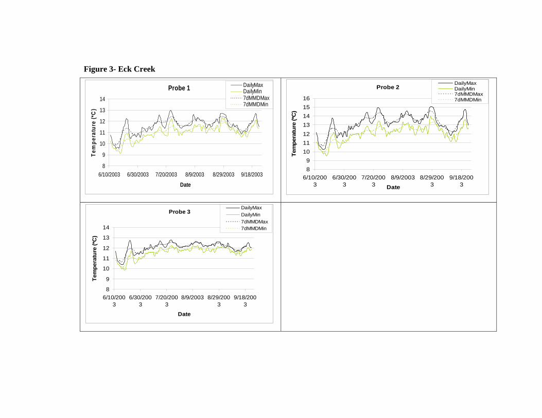
Figure 3- Eck Creek
Probe 1
8
9
10
11
12
13
14
6/10/2003 6/30/2003 7/20/2003 8/9/2003 8/29/2003 9/18/2003
Date
Tem
pera
ture
(*C
)DailyMaxDailyMin7dMMDMax7dMMDMin
Probe 2
89
10111213141516
6/10/2003
6/30/2003
7/20/2003
8/9/2003 8/29/2003
9/18/2003Date
Tem
pera
ture
(*C
)
DailyMaxDailyMin7dMMDMax7dMMDMin
Probe 3
8
9
10
11
12
13
14
6/10/2003
6/30/2003
7/20/2003
8/9/2003 8/29/2003
9/18/2003
Date
Tem
pera
ture
(*C
)
DailyMaxDailyMin7dMMDMax7dMMDMin
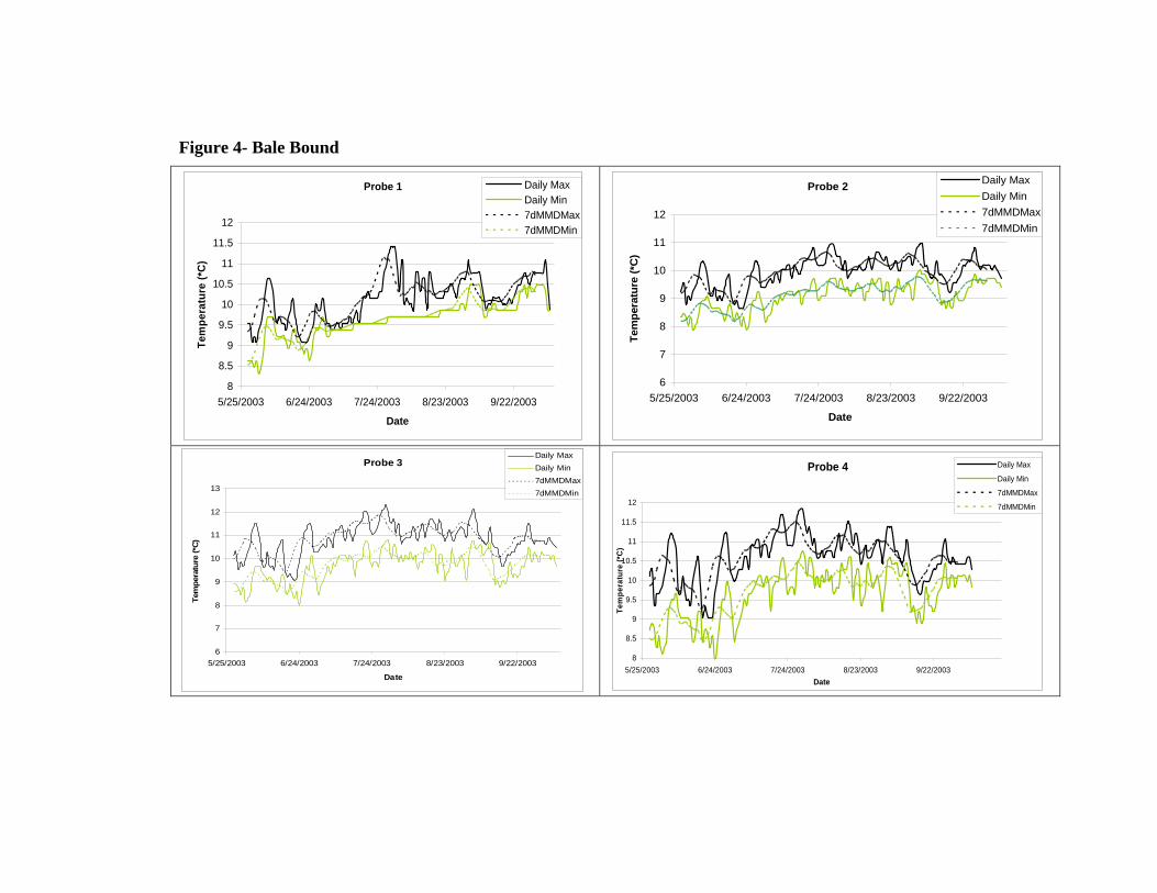
Figure 4- Bale Bound
Probe 1
8
8.5
9
9.5
10
10.5
11
11.5
12
5/25/2003 6/24/2003 7/24/2003 8/23/2003 9/22/2003
Date
Tem
pera
ture
(*C
)Daily MaxDaily Min7dMMDMax7dMMDMin
Probe 2
6
7
8
9
10
11
12
5/25/2003 6/24/2003 7/24/2003 8/23/2003 9/22/2003
Date
Tem
pera
ture
(*C
)
Daily MaxDaily Min7dMMDMax7dMMDMin
Probe 3
6
7
8
9
10
11
12
13
5/25/2003 6/24/2003 7/24/2003 8/23/2003 9/22/2003
Date
Tem
pera
ture
(*C)
Daily MaxDaily Min7dMMDMax7dMMDMin
Probe 4
8
8.5
9
9.5
10
10.5
11
11.5
12
5/25/2003 6/24/2003 7/24/2003 8/23/2003 9/22/2003Date
Tem
pera
ture
(*C
)
Daily Max
Daily Min
7dMMDMax
7dMMDMin
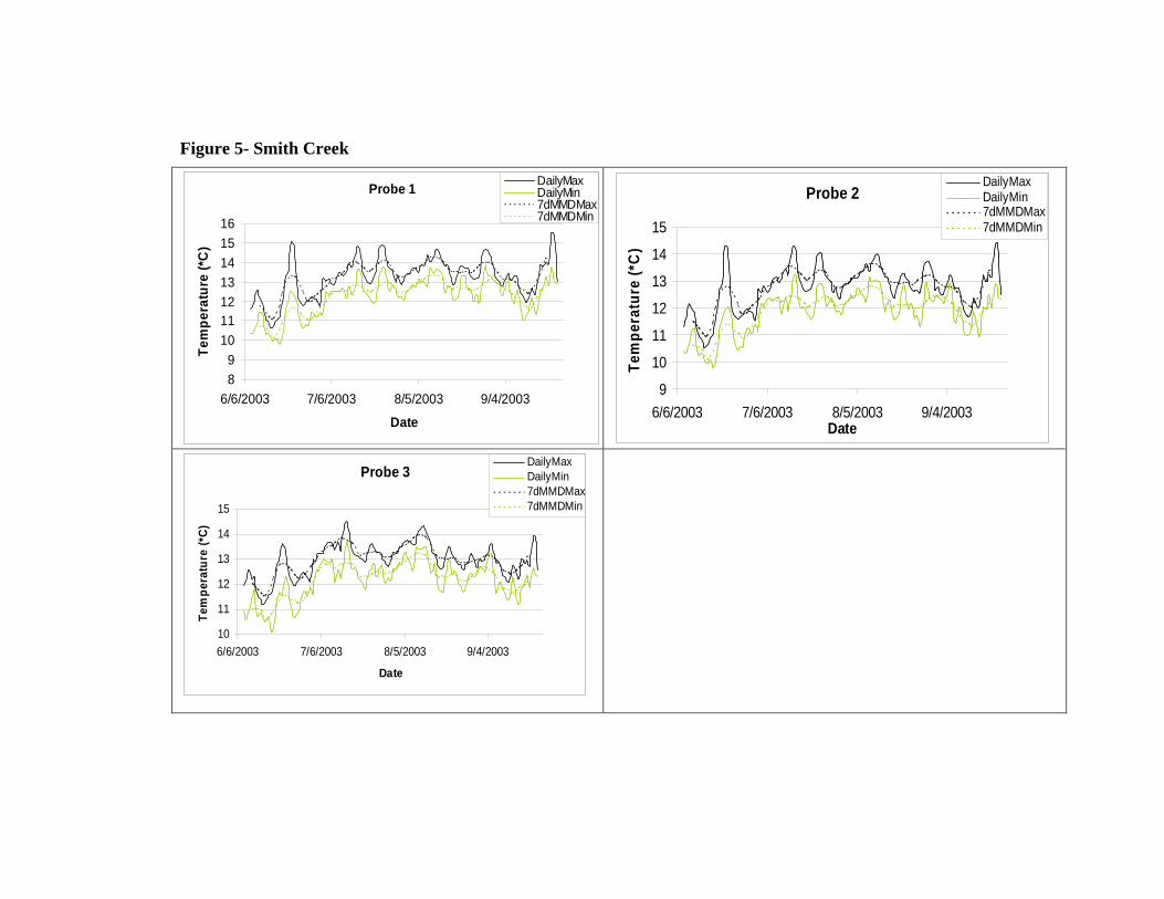
Figure 5- Smith Creek
Probe 1
89
10111213141516
6/6/2003 7/6/2003 8/5/2003 9/4/2003
Date
Tem
pera
ture
(*C
)DailyMaxDailyMin7dMMDMax7dMMDMin
Probe 2
9
10
11
12
13
14
15
6/6/2003 7/6/2003 8/5/2003 9/4/2003Date
Tem
pera
ture
(*C
)
DailyMaxDailyMin7dMMDMax7dMMDMin
Probe 3
10
11
12
13
14
15
6/6/2003 7/6/2003 8/5/2003 9/4/2003
Date
Tem
pera
ture
(*C)
DailyMaxDailyMin7dMMDMax7dMMDMin
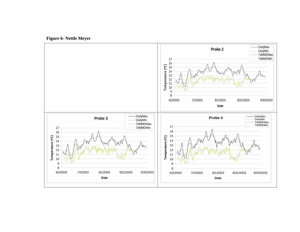
Figure 6- Nettle Meyer
Probe 2
89
1011121314151617
6/2/2003 7/2/2003 8/1/2003 8/31/2003 9/30/2003
Date
Tem
pera
ture
(*C
)
DailyMaxDailyMin7dMMDMax7dMMDMin
Probe 3
89
1011121314151617
6/2/2003 7/2/2003 8/1/2003 8/31/2003 9/30/2003
Date
Tem
pera
ture
(*C
)
DailyMaxDailyMin7dMMDMax7dMMDMin
Probe 4
89
1011121314151617
6/2/2003 7/2/2003 8/1/2003 8/31/2003 9/30/2003
Date
Tem
pera
ture
(*C
)
DailyMaxDailyMin7dMMDMax7dMMDMin
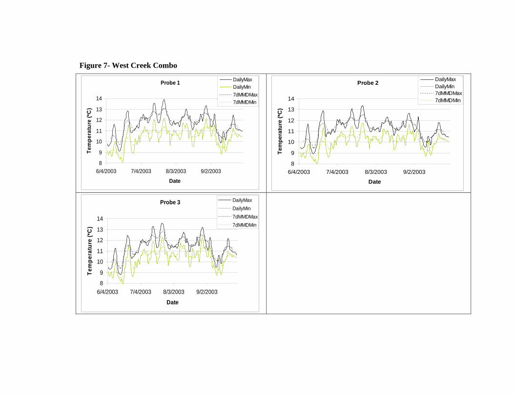
Figure 7- West Creek Combo
Probe 1
8
9
10
11
12
13
14
6/4/2003 7/4/2003 8/3/2003 9/2/2003
Date
Tem
pera
ture
(*C
)DailyMaxDailyMin7dMMDMax7dMMDMin
Probe 2
8
9
10
11
12
13
14
6/4/2003 7/4/2003 8/3/2003 9/2/2003
Date
Tem
pera
ture
(*C
)
DailyMaxDailyMin7dMMDMax7dMMDMin
Probe 3
8
9
10
11
12
13
14
6/4/2003 7/4/2003 8/3/2003 9/2/2003
Date
Tem
pera
ture
(*C
)
DailyMaxDailyMin7dMMDMax7dMMDMin
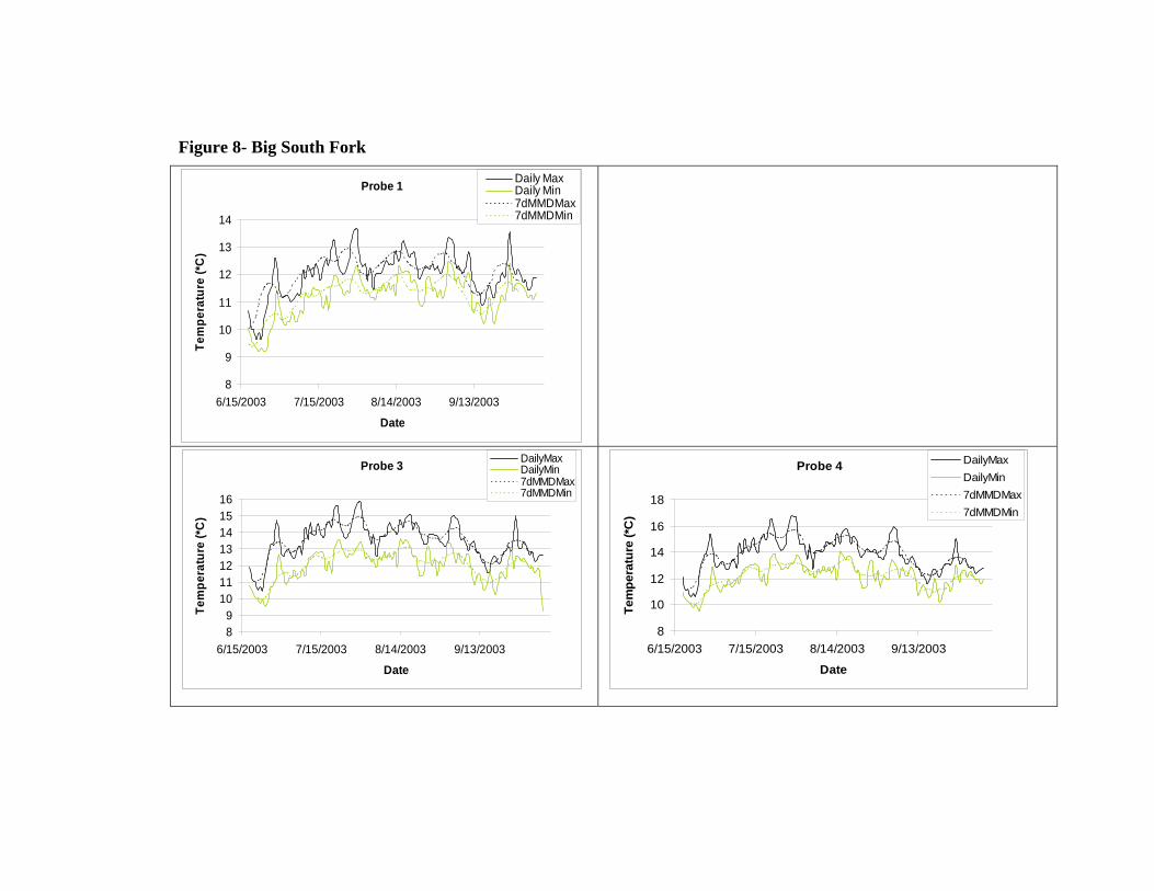
Figure 8- Big South Fork
Probe 1
8
9
10
11
12
13
14
6/15/2003 7/15/2003 8/14/2003 9/13/2003
Date
Tem
pera
ture
(*C
)
Daily MaxDaily Min7dMMDMax7dMMDMin
Probe 3
89
10111213141516
6/15/2003 7/15/2003 8/14/2003 9/13/2003
Date
Tem
pera
ture
(*C
)
DailyMaxDailyMin7dMMDMax7dMMDMin
Probe 4
8
10
12
14
16
18
6/15/2003 7/15/2003 8/14/2003 9/13/2003
Date
Tem
pera
ture
(*C
)
DailyMaxDailyMin7dMMDMax7dMMDMin
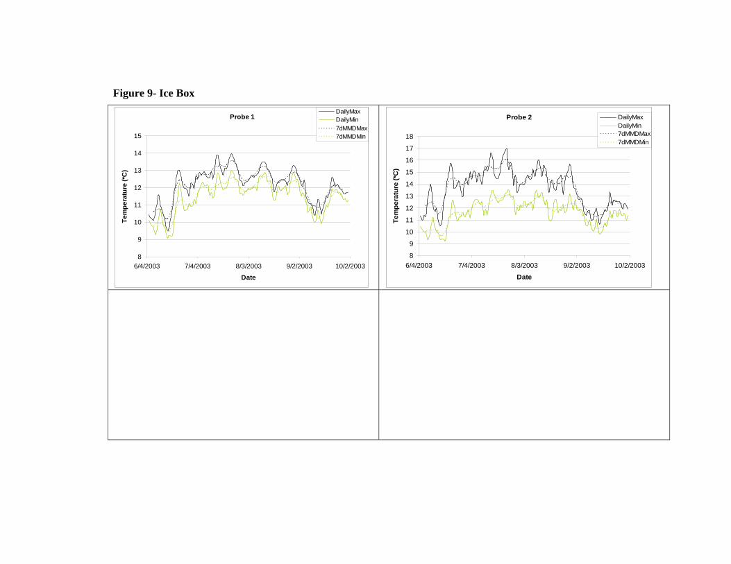
Figure 9- Ice Box
Probe 1
8
9
10
11
12
13
14
15
6/4/2003 7/4/2003 8/3/2003 9/2/2003 10/2/2003
Date
Tem
pera
ture
(*C
)
DailyMaxDailyMin7dMMDMax7dMMDMin
Probe 2
8
9
10
11
12
13
14
15
16
17
18
6/4/2003 7/4/2003 8/3/2003 9/2/2003 10/2/2003
Date
Tem
pera
ture
(*C
)
DailyMaxDailyMin7dMMDMax7dMMDMin

Figure 10- Shangrila
Probe 1
1011121314151617
6/5/2003 7/5/2003 8/4/2003 9/3/2003 10/3/2003
Date
Tem
pera
ture
(*C
)DailyMaxDailyMin7dMMDMax7dMMDMin
Probe 2
10
11
12
1314
15
16
17
6/5/2003 7/5/2003 8/4/2003 9/3/2003 10/3/2003
Date
Tem
pera
ture
(*C
)
DailyMaxDailyMin7dMMDMax7dMMDMin
Probe 3
10
11
12
13
14
15
16
17
6/5/2003 7/5/2003 8/4/2003 9/3/2003 10/3/2003
Date
Tem
pera
ture
(*C
)
DailyMaxDailyMin7dMMDMax7dMMDMin
Probe 4
1011121314151617
6/5/2003 6/25/2003
7/15/2003
8/4/2003 8/24/2003
9/13/2003
Date
Tem
pera
ture
(*C
)
DailyMaxDailyMin7dMMDMax7dMMDMin
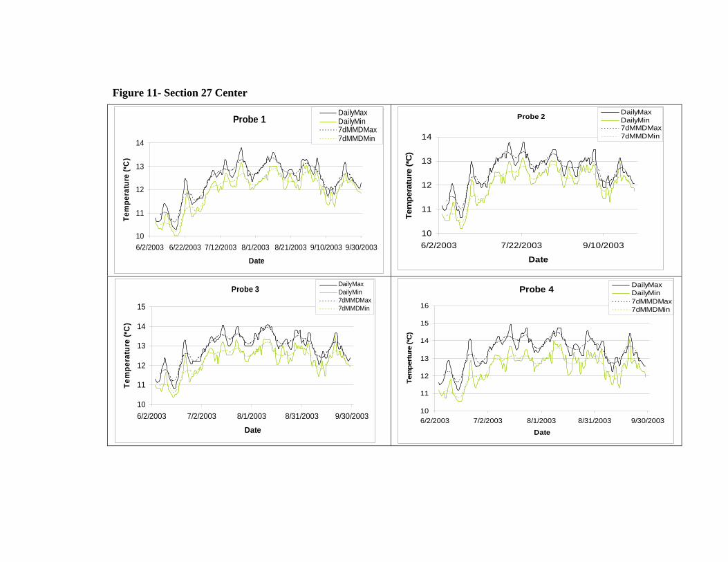
Figure 11- Section 27 Center
Probe 1
10
11
12
13
14
6/2/2003 6/22/2003 7/12/2003 8/1/2003 8/21/2003 9/10/2003 9/30/2003
Date
Tem
pera
ture
(*C
)
DailyMaxDailyMin7dMMDMax7dMMDMin
Probe 2
10
11
12
13
14
6/2/2003 7/22/2003 9/10/2003
Date
Tem
pera
ture
(*C
)
DailyMaxDailyMin7dMMDMax7dMMDMin
Probe 3
10
11
12
13
14
15
6/2/2003 7/2/2003 8/1/2003 8/31/2003 9/30/2003
Date
Tem
pera
ture
(*C
)
DailyMaxDailyMin7dMMDMax7dMMDMin
Probe 4
10
11
12
13
14
15
16
6/2/2003 7/2/2003 8/1/2003 8/31/2003 9/30/2003
Date
Tem
pertu
re (*
C)
DailyMaxDailyMin7dMMDMax7dMMDMin
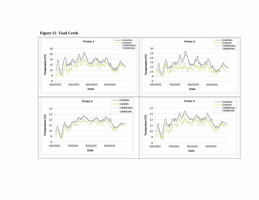
Figure 12- Toad Creek
Probe 1
6
8
10
12
14
16
18
6/6/2003 7/6/2003 8/5/2003 9/4/2003
Date
Tem
pera
ture
(*C
)
DailyMaxDailyMin7dMMDMax7dMMDMin
Probe 2
6
8
10
12
14
16
18
20
6/6/2003 7/6/2003 8/5/2003 9/4/2003
Date
Tem
pera
ture
(*C
)
DailyMaxDailyMin7dMMDMax7dMMDMin
Probe 3
8
9
10
11
12
13
14
6/6/2003 7/6/2003 8/5/2003 9/4/2003
Date
Tem
pera
ture
(*C
)
DailyMaxDailyMin7dMMDMax7dMMDMin
Probe 4
8
9
10
11
12
13
14
6/6/2003 7/6/2003 8/5/2003 9/4/2003
Date
Tem
pera
ture
(*C
)
DailyMaxDailyMin7dMMDMax7dMMDMin
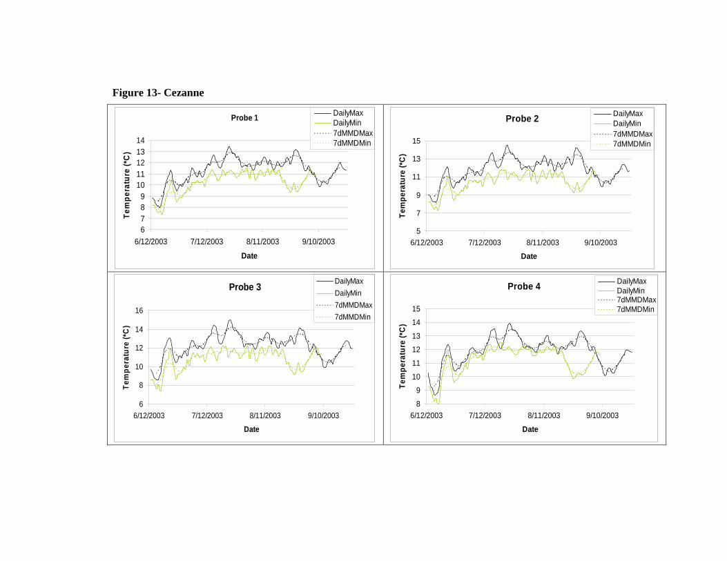
Figure 13- Cezanne
Probe 1
6789
1011121314
6/12/2003 7/12/2003 8/11/2003 9/10/2003
Date
Tem
pera
ture
(*C
)DailyMaxDailyMin7dMMDMax7dMMDMin
Probe 2
5
7
9
11
13
15
6/12/2003 7/12/2003 8/11/2003 9/10/2003
Date
Tem
pera
ture
(*C
)
DailyMaxDailyMin7dMMDMax7dMMDMin
Probe 3
6
8
10
12
14
16
6/12/2003 7/12/2003 8/11/2003 9/10/2003
Date
Tem
pera
ture
(*C
)
DailyMaxDailyMin7dMMDMax7dMMDMin
Probe 4
8
9
10
11
12
13
14
15
6/12/2003 7/12/2003 8/11/2003 9/10/2003
Date
Tem
pera
ture
(*C
)
DailyMaxDailyMin7dMMDMax7dMMDMin

Figure 14- South Fork Trask
Probe 1
6
8
10
12
14
16
18
6/18/2003 7/18/2003 8/17/2003 9/16/2003Date
Tem
pera
ture
(*C
)DailyMaxDailyMin7dMMDMax7dMMDMin
Probe 2
6789
1011121314
6/18/2003 7/18/2003 8/17/2003 9/16/2003Date
Tem
pera
ture
(*C
)
DailyMaxDailyMin7dMMDMax7dMMDMin
Probe 3
6789
1011121314
6/18/2003 7/18/2003 8/17/2003 9/16/2003
Date
Tem
pera
ture
DailyMaxDailyMin7dMMDMax7dMMDMin
Probe 4
6
8
10
12
14
16
6/18/2003 7/18/2003 8/17/2003 9/16/2003
DateTe
mpe
ratu
re (*
C)
DailyMaxDailyMin7dMMDMax7dMMDMin
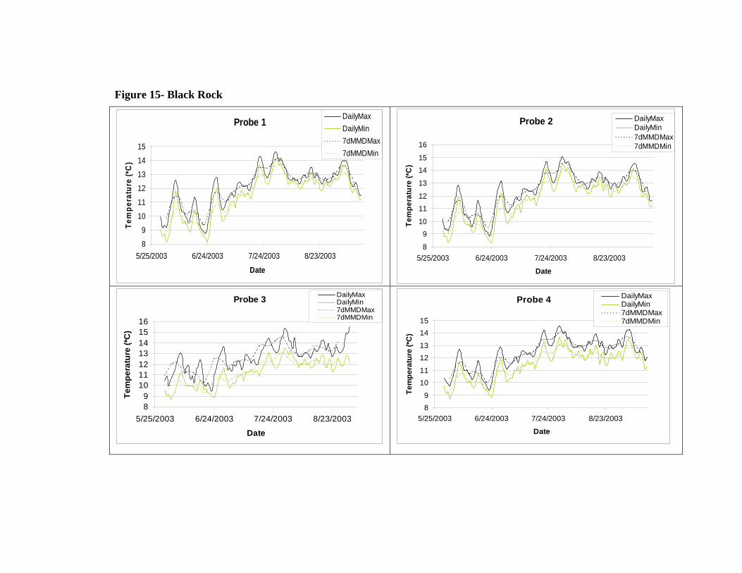
Figure 15- Black Rock
Probe 1
8
9
10
11
12
13
14
15
5/25/2003 6/24/2003 7/24/2003 8/23/2003
Date
Tem
pera
ture
(*C
)DailyMaxDailyMin7dMMDMax7dMMDMin
Probe 2
8
910
1112
13
1415
16
5/25/2003 6/24/2003 7/24/2003 8/23/2003
Date
Tem
pera
ture
(*C
)
DailyMaxDailyMin7dMMDMax7dMMDMin
Probe 3
89
10111213141516
5/25/2003 6/24/2003 7/24/2003 8/23/2003
Date
Tem
pera
ture
(*C
)
DailyMaxDailyMin7dMMDMax7dMMDMin
Probe 4
89
1011
1213
1415
5/25/2003 6/24/2003 7/24/2003 8/23/2003
Date
Tem
pera
ture
(*C
)
DailyMaxDailyMin7dMMDMax7dMMDMin

Figure 16- Bridge 40 Creek
Probe 1
5
6
7
8
9
10
6/15/2003 7/5/2003 7/25/2003 8/14/2003 9/3/2003
Date
Tem
pera
ture
(*C
)
DailyMaxDailyMin7dMMDMax7dMMDMin
Probe 2
5
6
7
8
9
10
11
12
6/18/2003 7/8/2003 7/28/2003 8/17/2003 9/6/2003
Date
Tem
pera
ture
(*C
)
DailyMaxDaily Min7dMMDMax7dMMDMin
Probe 3
6
7
8
9
10
11
12
13
14
6/18/2003 7/18/2003 8/17/2003 9/16/2003
Date
Tem
pera
ture
(*C
)
DailyMaxDailyMin7dMMDMax7dMMDMin
Probe 4
6789
1011121314
6/18/2003 7/8/2003 7/28/2003 8/17/2003 9/6/2003
Date
Tem
pera
ture
(*C
)
DailyMaxDailyMin7dMMDMax7dMMDMin
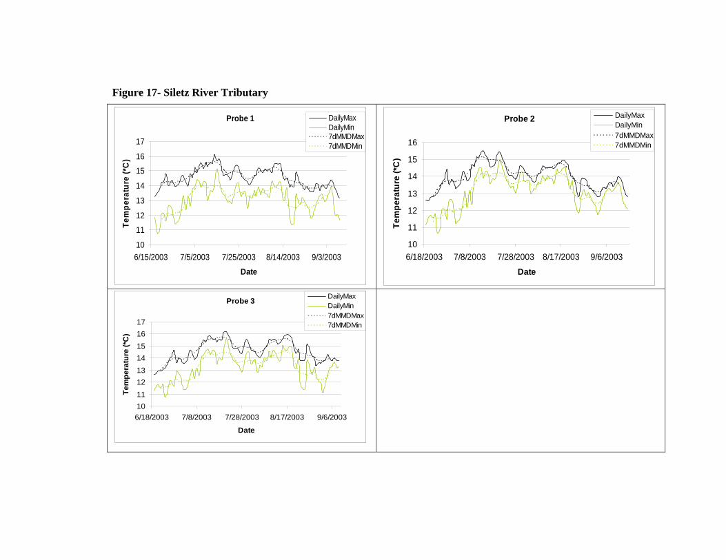
Figure 17- Siletz River Tributary
Probe 1
10
11
12
13
14
15
16
17
6/15/2003 7/5/2003 7/25/2003 8/14/2003 9/3/2003
Date
Tem
pera
ture
(*C
)DailyMaxDailyMin7dMMDMax7dMMDMin
Probe 2
10
11
12
13
14
15
16
6/18/2003 7/8/2003 7/28/2003 8/17/2003 9/6/2003
Date
Tem
pera
ture
(*C
)
DailyMaxDailyMin7dMMDMax7dMMDMin
Probe 3
1011121314151617
6/18/2003 7/8/2003 7/28/2003 8/17/2003 9/6/2003
Date
Tem
pera
ture
(*C
)
DailyMaxDailyMin7dMMDMax7dMMDMin
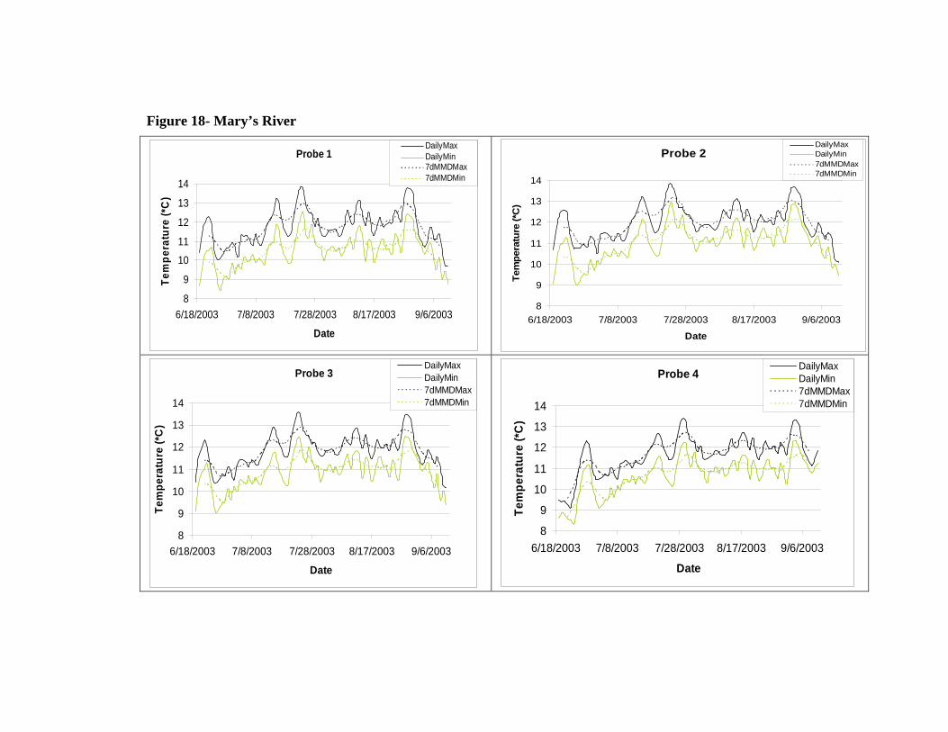
Figure 18- Mary’s River
Probe 1
8
9
10
11
12
13
14
6/18/2003 7/8/2003 7/28/2003 8/17/2003 9/6/2003
Date
Tem
pera
ture
(*C
)
DailyMaxDailyMin7dMMDMax7dMMDMin
Probe 2
8
9
10
11
12
13
14
6/18/2003 7/8/2003 7/28/2003 8/17/2003 9/6/2003
Date
Tem
pera
ture
(*C
)
DailyMaxDailyMin7dMMDMax7dMMDMin
Probe 3
8
9
10
11
12
13
14
6/18/2003 7/8/2003 7/28/2003 8/17/2003 9/6/2003
Date
Tem
pera
ture
(*C
)
DailyMaxDailyMin7dMMDMax7dMMDMin
Probe 4
8
9
10
11
12
13
14
6/18/2003 7/8/2003 7/28/2003 8/17/2003 9/6/2003
Date
Tem
pera
ture
(*C
)
DailyMaxDailyMin7dMMDMax7dMMDMin
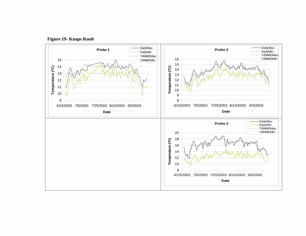
Figure 19- Knaps Knob
Probe 1
9
10
11
12
13
14
15
6/15/2003 7/5/2003 7/25/2003 8/14/2003 9/3/2003
Date
Tem
pera
ture
(*C
)DailyMaxDailyMin7dMMDMax7dMMDMin
Probe 2
89
10111213141516
6/15/2003 7/5/2003 7/25/2003 8/14/2003 9/3/2003
Date
Tem
pera
ture
(*C
)
DailyMaxDailyMin7dMMDMax7dMMDMin
Probe 4
8
10
12
14
16
18
20
6/15/2003 7/5/2003 7/25/2003 8/14/2003 9/3/2003
Date
Tem
pera
ture
(*C
)
DailyMaxDailyMin7dMMDMax7dMMDMin
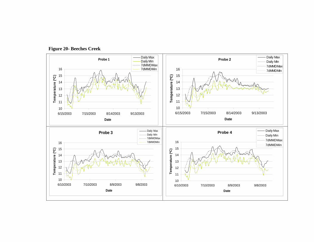
Figure 20- Beeches Creek
Probe 1
10
11
12
13
14
15
16
6/15/2003 7/15/2003 8/14/2003 9/13/2003
Date
Tem
pera
ture
(*C
)Daily MaxDaily Min7dMMDMax7dMMDMin
Probe 2
10
11
12
13
14
15
16
6/15/2003 7/15/2003 8/14/2003 9/13/2003
Date
Tem
pera
ture
(*C
)
Daily MaxDaily Min7dMMDMax7dMMDMin
Probe 3
10
11
12
13
14
15
16
6/10/2003 7/10/2003 8/9/2003 9/8/2003
Date
Tem
pera
ture
(*C
)
Daily MaxDaily Min7dMMDMax7dMMDMin
Probe 4
10
11
12
13
14
15
16
6/10/2003 7/10/2003 8/9/2003 9/8/2003
Date
Tem
pera
ture
(*C
)
Daily MaxDaily Min7dMMDMax7dMMDMin
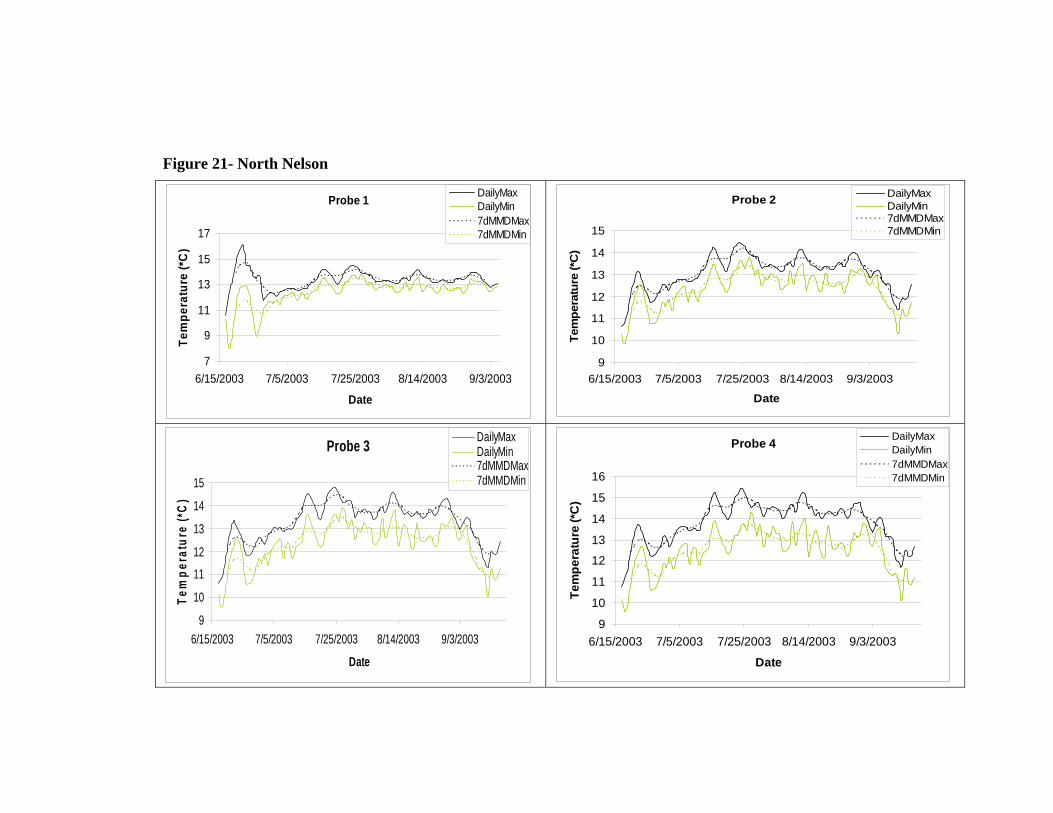
Figure 21- North Nelson
Probe 1
7
9
11
13
15
17
6/15/2003 7/5/2003 7/25/2003 8/14/2003 9/3/2003
Date
Tem
pera
ture
(*C
)DailyMaxDailyMin7dMMDMax7dMMDMin
Probe 2
9
10
11
12
13
14
15
6/15/2003 7/5/2003 7/25/2003 8/14/2003 9/3/2003
Date
Tem
pera
ture
(*C
)
DailyMaxDailyMin7dMMDMax7dMMDMin
Probe 3
9
10
11
12
13
14
15
6/15/2003 7/5/2003 7/25/2003 8/14/2003 9/3/2003
Date
Tem
pera
ture
(*C
)
DailyMaxDailyMin7dMMDMax7dMMDMin
Probe 4
9
10
11
12
13
14
15
16
6/15/2003 7/5/2003 7/25/2003 8/14/2003 9/3/2003
Date
Tem
pera
ture
(*C
)
DailyMaxDailyMin7dMMDMax7dMMDMin
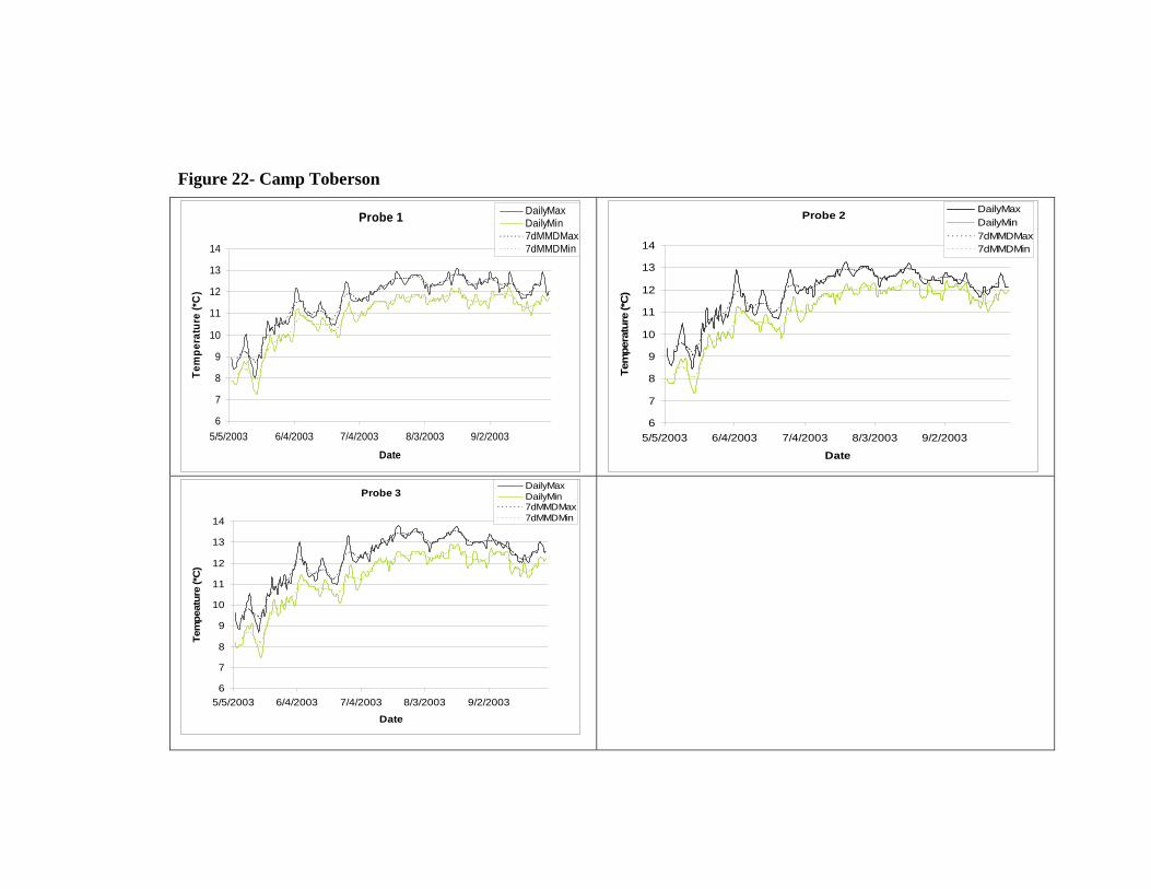
Figure 22- Camp Toberson
Probe 1
6
7
8
9
10
11
12
13
14
5/5/2003 6/4/2003 7/4/2003 8/3/2003 9/2/2003
Date
Tem
pera
ture
(*C
)DailyMaxDailyMin7dMMDMax7dMMDMin
Probe 2
6
7
8
9
10
11
12
13
14
5/5/2003 6/4/2003 7/4/2003 8/3/2003 9/2/2003
Date
Tem
pera
ture
(*C
)
DailyMaxDailyMin7dMMDMax7dMMDMin
Probe 3
6
7
8
9
10
11
12
13
14
5/5/2003 6/4/2003 7/4/2003 8/3/2003 9/2/2003
Date
Tem
peat
ure
(*C
)
DailyMaxDailyMin7dMMDMax7dMMDMin
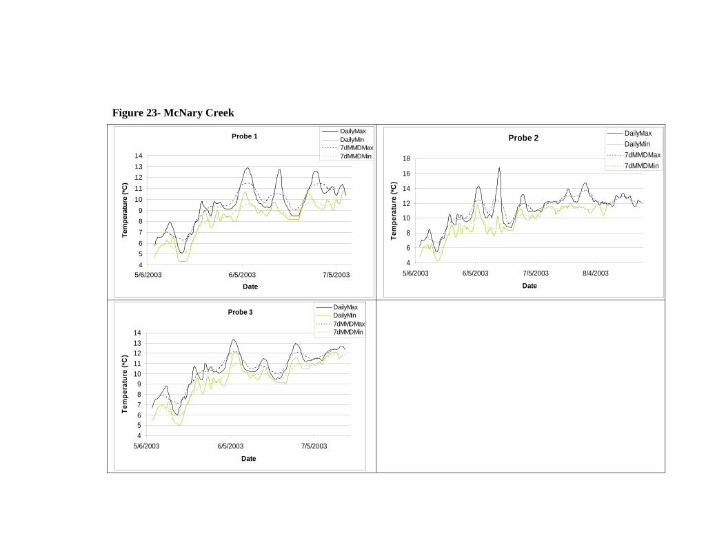
Figure 23- McNary Creek
Probe 1
456789
1011121314
5/6/2003 6/5/2003 7/5/2003
Date
Tem
pera
ture
(*C
)DailyMaxDailyMin7dMMDMax7dMMDMin
Probe 2
4
6
8
10
12
14
16
18
5/6/2003 6/5/2003 7/5/2003 8/4/2003
Date
Tem
pera
ture
(*C
)
DailyMaxDailyMin7dMMDMax7dMMDMin
Probe 3
456789
1011121314
5/6/2003 6/5/2003 7/5/2003
Date
Tem
pera
ture
(*C
)
DailyMaxDailyMin7dMMDMax7dMMDMin
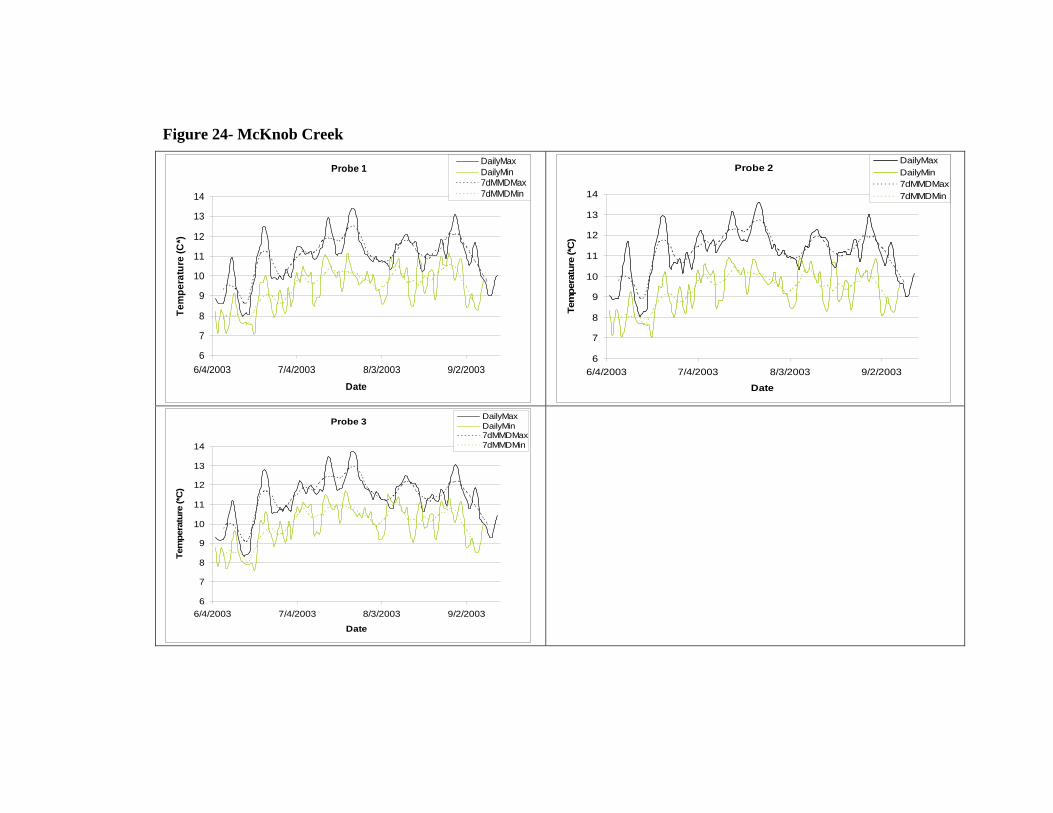
Figure 24- McKnob Creek
Probe 1
6
7
8
9
10
11
12
13
14
6/4/2003 7/4/2003 8/3/2003 9/2/2003
Date
Tem
pera
ture
(C*)
DailyMaxDailyMin7dMMDMax7dMMDMin
Probe 2
6
7
8
9
10
11
12
13
14
6/4/2003 7/4/2003 8/3/2003 9/2/2003
Date
Tem
pera
ture
(*C
)
DailyMaxDailyMin7dMMDMax7dMMDMin
Probe 3
6
7
8
9
10
11
12
13
14
6/4/2003 7/4/2003 8/3/2003 9/2/2003
Date
Tem
pera
ture
(*C
)
DailyMaxDailyMin7dMMDMax7dMMDMin
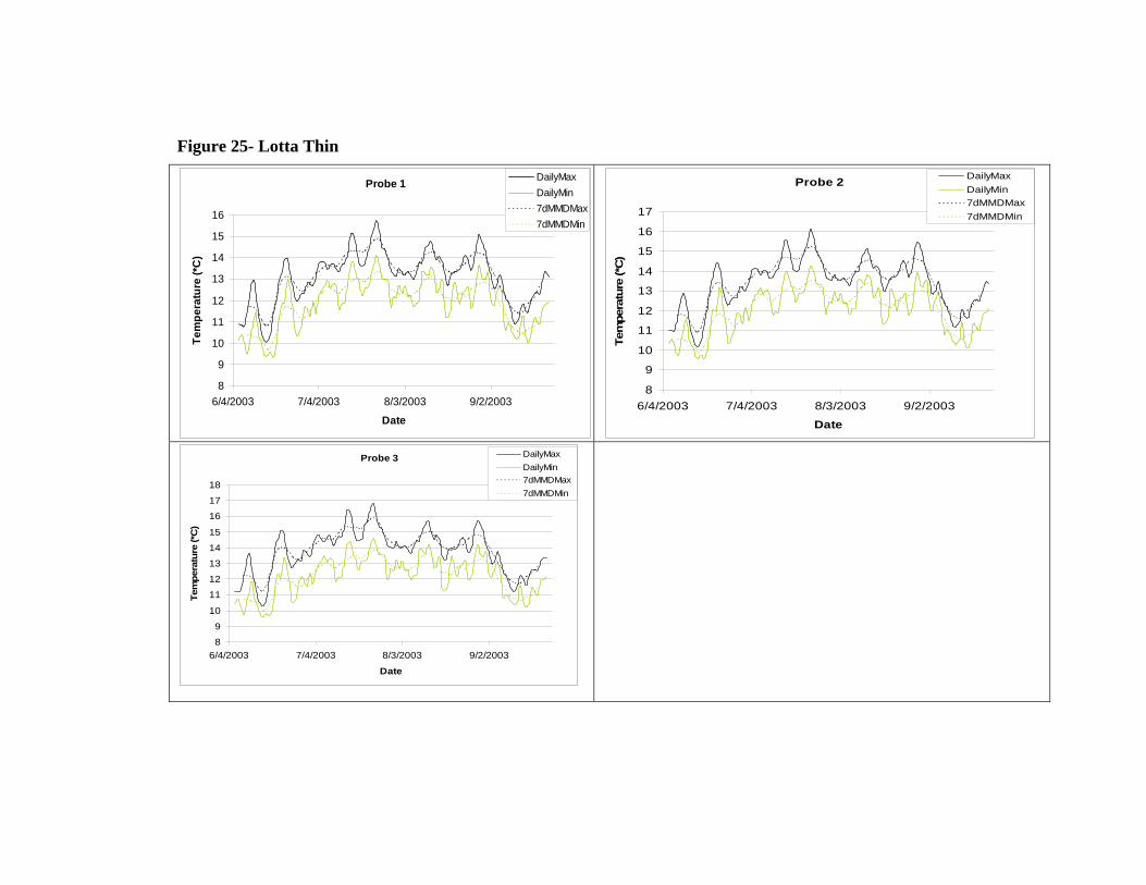
Figure 25- Lotta Thin
Probe 1
8
9
10
11
12
13
14
15
16
6/4/2003 7/4/2003 8/3/2003 9/2/2003
Date
Tem
pera
ture
(*C
)
DailyMaxDailyMin7dMMDMax7dMMDMin
Probe 2
8
9
10
11
12
13
14
15
16
17
6/4/2003 7/4/2003 8/3/2003 9/2/2003
Date
Tem
pera
ture
(*C
)
DailyMaxDailyMin7dMMDMax7dMMDMin
Probe 3
8
9
10
11
12
13
14
15
16
17
18
6/4/2003 7/4/2003 8/3/2003 9/2/2003
Date
Tem
pera
ture
(*C
)
DailyMaxDailyMin7dMMDMax7dMMDMin
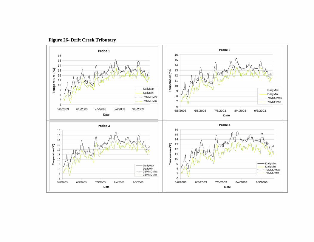
Figure 26- Drift Creek Tributary
Probe 1
6789
10111213141516
5/6/2003 6/5/2003 7/5/2003 8/4/2003 9/3/2003
Date
Tem
pera
ture
(*C
)
DailyMaxDailyMin7dMMDMax7dMMDMin
Probe 2
6
7
8
9
10
11
12
13
14
15
16
5/6/2003 6/5/2003 7/5/2003 8/4/2003 9/3/2003
Date
Tem
pera
ture
(*C
)
DailyMaxDailyMin7dMMDMax7dMMDMin
Probe 3
6
7
8
9
10
11
12
13
14
15
16
5/6/2003 6/5/2003 7/5/2003 8/4/2003 9/3/2003
Date
Tem
pera
ture
(*C
)
DailyMaxDailyMin7dMMDMax7dMMDMin
Probe 4
6
7
8
9
10
11
12
13
14
15
16
5/6/2003 6/5/2003 7/5/2003 8/4/2003 9/3/2003
Date
Tem
pera
ture
(*C
)
DailyMaxDailyMin7dMMDMax7dMMDMin
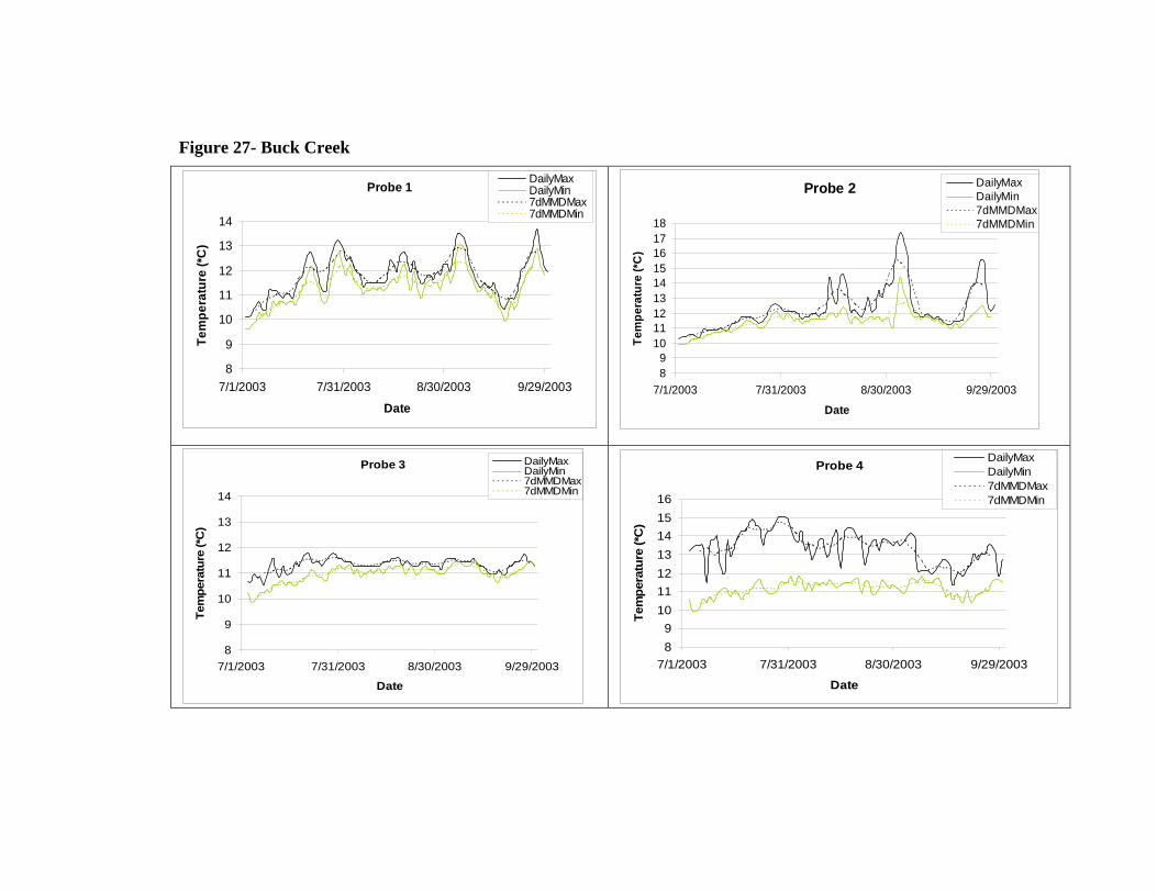
Figure 27- Buck Creek
Probe 1
8
9
10
11
12
13
14
7/1/2003 7/31/2003 8/30/2003 9/29/2003
Date
Tem
pera
ture
(*C
)
DailyMaxDailyMin7dMMDMax7dMMDMin
Probe 2
89
101112131415161718
7/1/2003 7/31/2003 8/30/2003 9/29/2003
Date
Tem
pera
ture
(*C
)
DailyMaxDailyMin7dMMDMax7dMMDMin
Probe 3
8
9
10
11
12
13
14
7/1/2003 7/31/2003 8/30/2003 9/29/2003
Date
Tem
pera
ture
(*C
)
DailyMaxDailyMin7dMMDMax7dMMDMin
Probe 4
89
10111213141516
7/1/2003 7/31/2003 8/30/2003 9/29/2003
Date
Tem
pera
ture
(*C
)
DailyMaxDailyMin7dMMDMax7dMMDMin
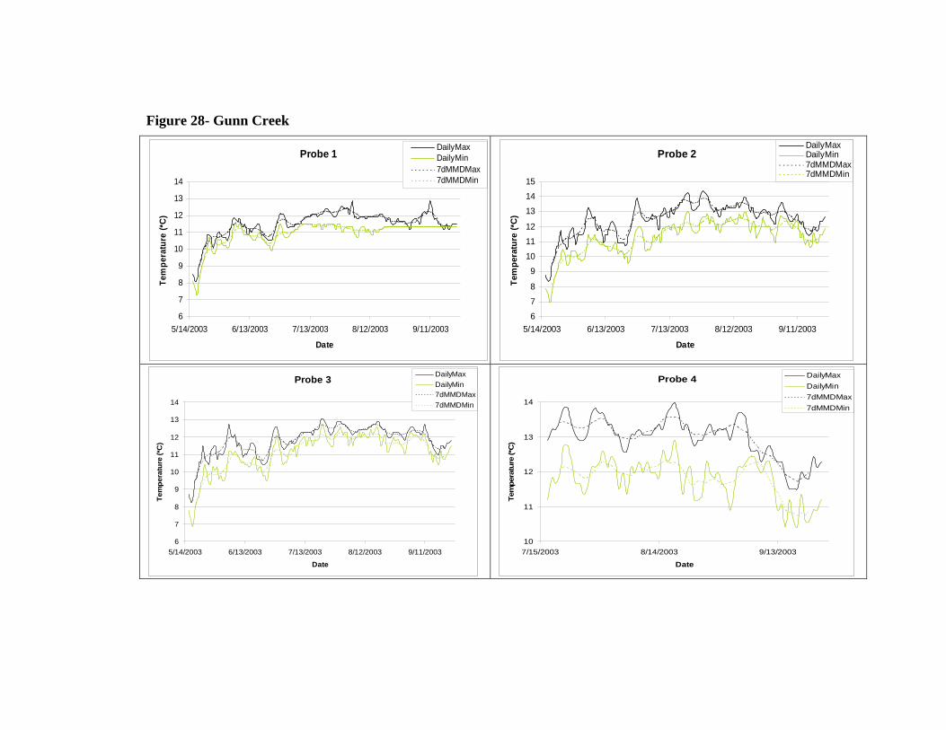
Figure 28- Gunn Creek
Probe 1
6
7
8
9
10
11
12
13
14
5/14/2003 6/13/2003 7/13/2003 8/12/2003 9/11/2003
Date
Tem
pera
ture
(*C
)
DailyMaxDailyMin7dMMDMax7dMMDMin
Probe 2
6
7
8
9
10
11
12
13
14
15
5/14/2003 6/13/2003 7/13/2003 8/12/2003 9/11/2003
Date
Tem
pera
ture
(*C
)
DailyMaxDailyMin7dMMDMax7dMMDMin
Probe 3
6
7
8
9
10
11
12
13
14
5/14/2003 6/13/2003 7/13/2003 8/12/2003 9/11/2003
Date
Tem
pera
ture
(*C
)
DailyMaxDailyMin7dMMDMax7dMMDMin
Probe 4
10
11
12
13
14
7/15/2003 8/14/2003 9/13/2003
Date
Tem
pera
ture
(*C
)
DailyMaxDailyMin7dMMDMax7dMMDMin

Figure 29- Elk Creek North
Probe 1
6
8
10
12
14
16
18
5/14/2003 6/13/2003 7/13/2003
Date
Tem
pera
ture
(*C)
DailyMaxDailyMin7dMMDMax7dMMDMin
Probe 3
6
7
8
9
10
11
12
13
5/14/2003 6/13/2003 7/13/2003
Date
Tem
pera
ture
(*C
)
DailyMaxDailyMin7dMMDMax7dMMDMin
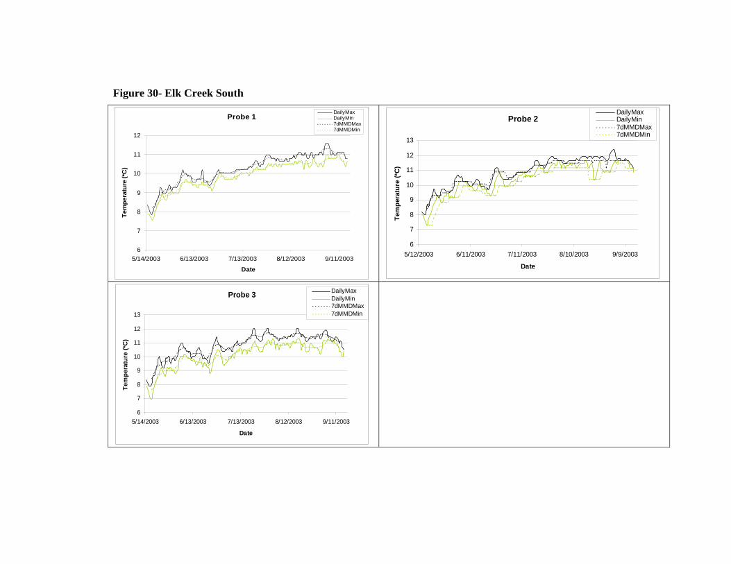
Figure 30- Elk Creek South
Probe 1
6
7
8
9
10
11
12
5/14/2003 6/13/2003 7/13/2003 8/12/2003 9/11/2003
Date
Tem
pera
ture
(*C
)
DailyMaxDailyMin7dMMDMax7dMMDMin
Probe 2
6
7
8
9
10
11
12
13
5/12/2003 6/11/2003 7/11/2003 8/10/2003 9/9/2003
Date
Tem
pera
ture
(*C
)
DailyMaxDailyMin7dMMDMax7dMMDMin
Probe 3
6
7
8
9
10
11
12
13
5/14/2003 6/13/2003 7/13/2003 8/12/2003 9/11/2003
Date
Tem
pera
ture
(*C
)
DailyMaxDailyMin7dMMDMax7dMMDMin
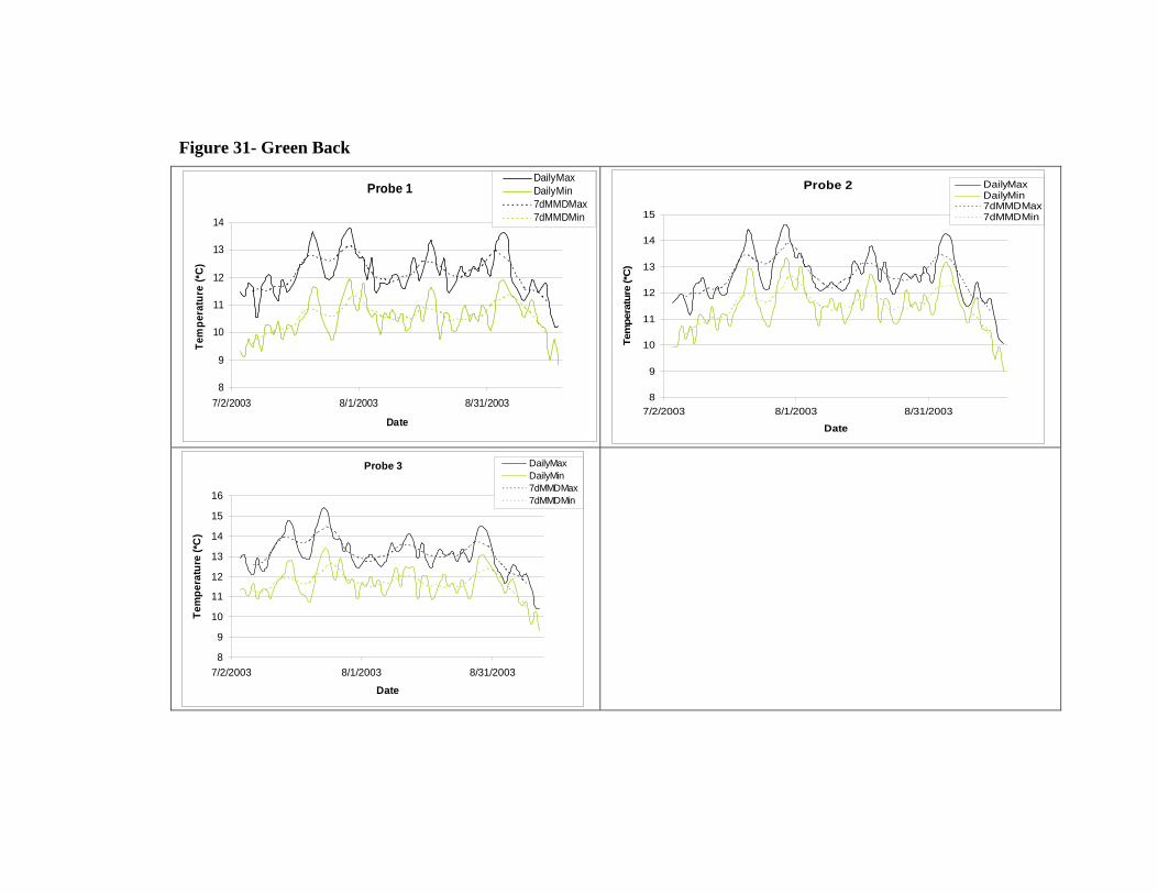
Figure 31- Green Back
Probe 1
8
9
10
11
12
13
14
7/2/2003 8/1/2003 8/31/2003
Date
Tem
pera
ture
(*C
)
DailyMaxDailyMin7dMMDMax7dMMDMin
Probe 2
8
9
10
11
12
13
14
15
7/2/2003 8/1/2003 8/31/2003
Date
Tem
pera
ture
(*C
)
DailyMaxDailyMin7dMMDMax7dMMDMin
Probe 3
8
9
10
11
12
13
14
15
16
7/2/2003 8/1/2003 8/31/2003
Date
Tem
pera
ture
(*C
)
DailyMaxDailyMin7dMMDMax7dMMDMin
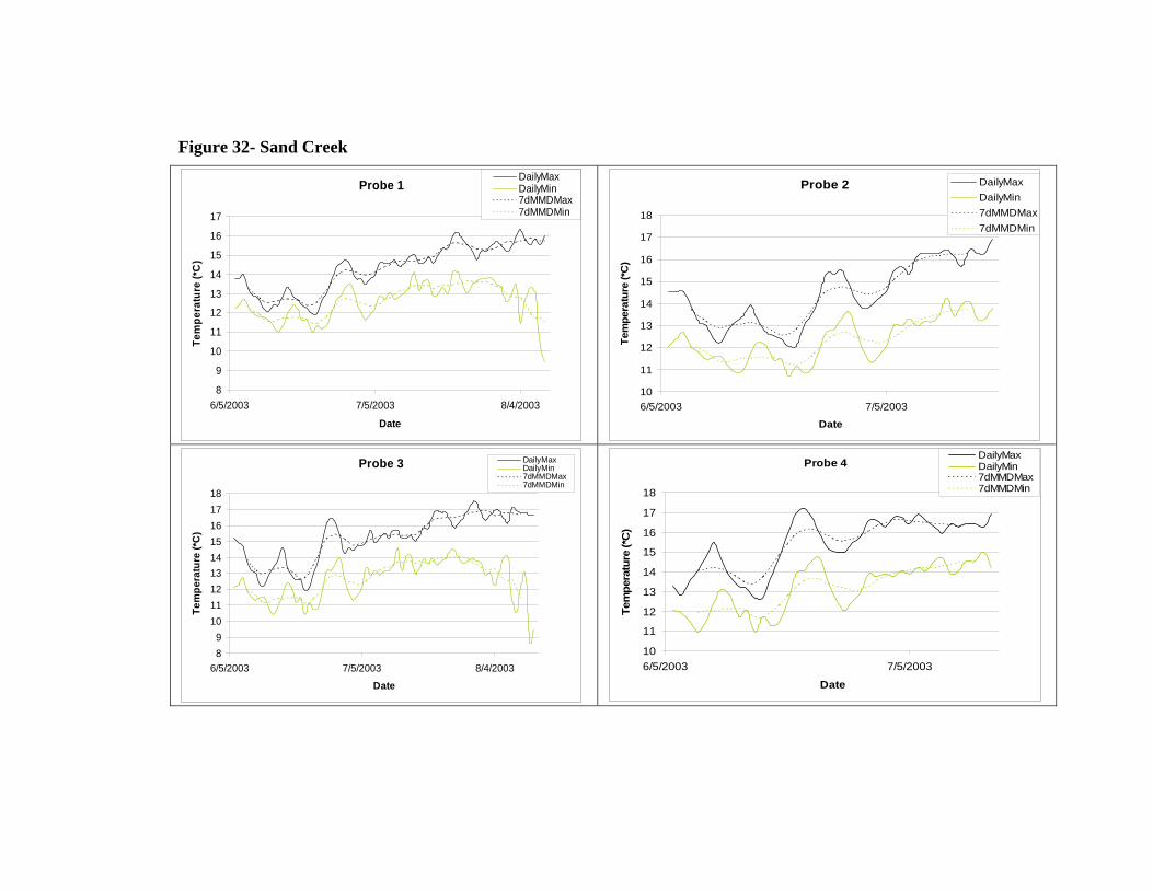
Figure 32- Sand Creek
Probe 1
8
9
10
11
12
13
14
15
16
17
6/5/2003 7/5/2003 8/4/2003
Date
Tem
pera
ture
(*C
)
DailyMaxDailyMin7dMMDMax7dMMDMin
Probe 2
10
11
12
13
14
15
16
17
18
6/5/2003 7/5/2003
Date
Tem
pera
ture
(*C
)
DailyMaxDailyMin7dMMDMax7dMMDMin
Probe 3
89
101112131415161718
6/5/2003 7/5/2003 8/4/2003
Date
Tem
pera
ture
(*C
)
DailyMaxDailyMin7dMMDMax7dMMDMin
Probe 4
10
11
12
13
14
15
16
17
18
6/5/2003 7/5/2003
Date
Tem
pera
ture
(*C
)
DailyMaxDailyMin7dMMDMax7dMMDMin
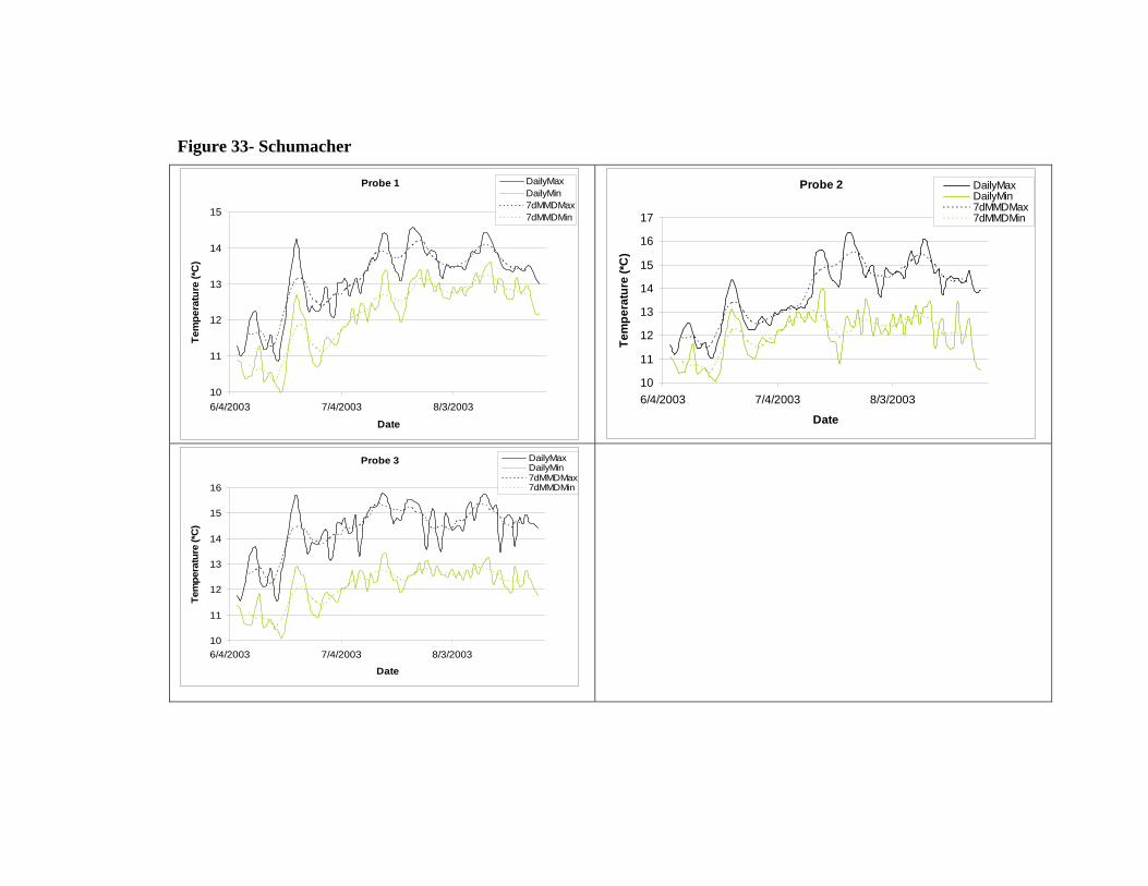
Figure 33- Schumacher
Probe 1
10
11
12
13
14
15
6/4/2003 7/4/2003 8/3/2003
Date
Tem
pera
ture
(*C
)DailyMaxDailyMin7dMMDMax7dMMDMin
Probe 2
10
11
12
13
14
15
16
17
6/4/2003 7/4/2003 8/3/2003
Date
Tem
pera
ture
(*C
)
DailyMaxDailyMin7dMMDMax7dMMDMin
Probe 3
10
11
12
13
14
15
16
6/4/2003 7/4/2003 8/3/2003
Date
Tem
pera
ture
(*C
)
DailyMaxDailyMin7dMMDMax7dMMDMin
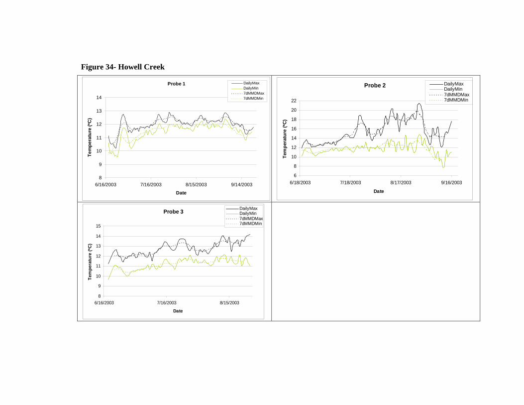
Figure 34- Howell Creek
Probe 1
8
9
10
11
12
13
14
6/16/2003 7/16/2003 8/15/2003 9/14/2003
Date
Tem
pera
ture
(*C
)DailyMaxDailyMin7dMMDMax7dMMDMin
Probe 2
6
8
10
12
14
16
18
20
22
6/18/2003 7/18/2003 8/17/2003 9/16/2003
Date
Tem
pera
ture
(*C
)
DailyMaxDailyMin7dMMDMax7dMMDMin
Probe 3
8
9
10
11
12
13
14
15
6/16/2003 7/16/2003 8/15/2003
Date
Tem
pera
ture
(*C
)
DailyMaxDailyMin7dMMDMax7dMMDMin
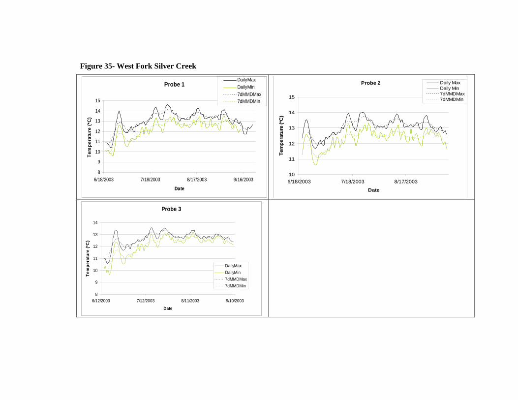
Figure 35- West Fork Silver Creek
Probe 1
8
9
10
11
12
13
14
15
6/18/2003 7/18/2003 8/17/2003 9/16/2003
Date
Tem
pera
ture
(*C)
DailyMaxDailyMin7dMMDMax7dMMDMin
Probe 2
10
11
12
13
14
15
6/18/2003 7/18/2003 8/17/2003
Date
Tem
pera
ture
(*C
)
Daily MaxDaily Min7dMMDMax7dMMDMin
Probe 3
8
9
10
11
12
13
14
6/12/2003 7/12/2003 8/11/2003 9/10/2003
Date
Tem
pera
ture
(*C
)
DailyMaxDailyMin7dMMDMax7dMMDMin
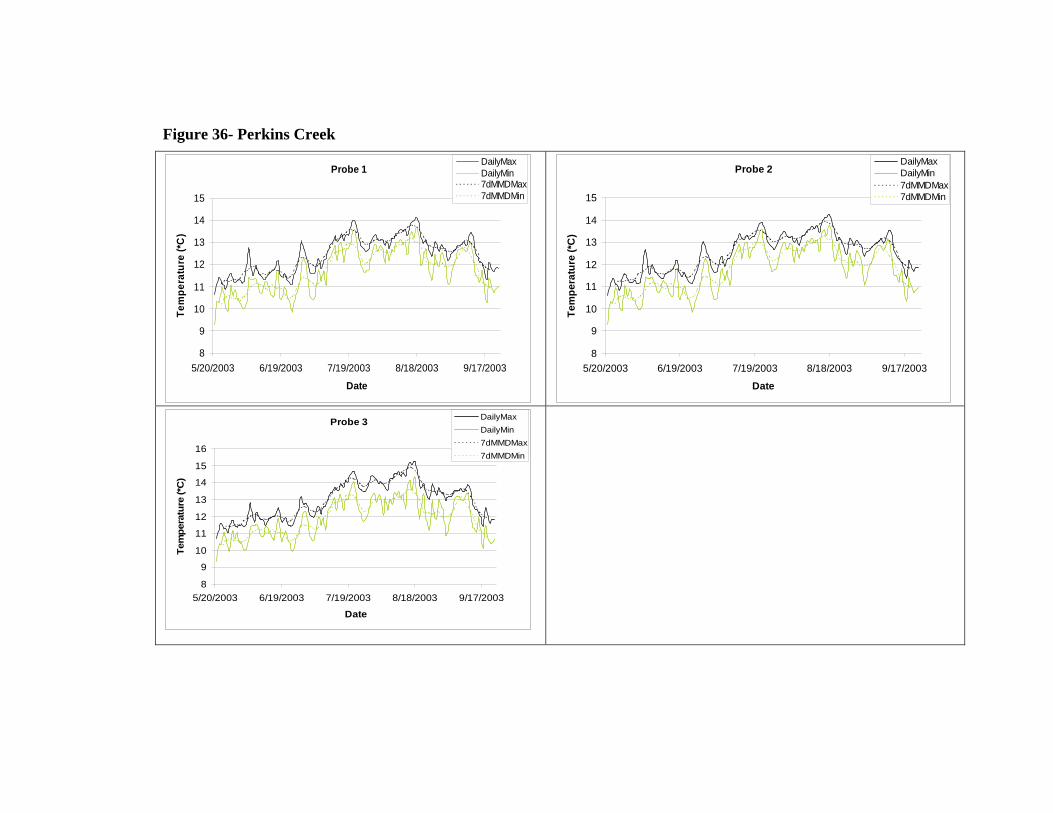
Figure 36- Perkins Creek
Probe 1
8
9
10
11
12
13
14
15
5/20/2003 6/19/2003 7/19/2003 8/18/2003 9/17/2003
Date
Tem
pera
ture
(*C
)
DailyMaxDailyMin7dMMDMax7dMMDMin
Probe 2
8
9
10
11
12
13
14
15
5/20/2003 6/19/2003 7/19/2003 8/18/2003 9/17/2003
Date
Tem
pera
ture
(*C
)
DailyMaxDailyMin7dMMDMax7dMMDMin
Probe 3
8
9
10
11
12
13
14
15
16
5/20/2003 6/19/2003 7/19/2003 8/18/2003 9/17/2003
Date
Tem
pera
ture
(*C
)
DailyMaxDailyMin7dMMDMax7dMMDMin
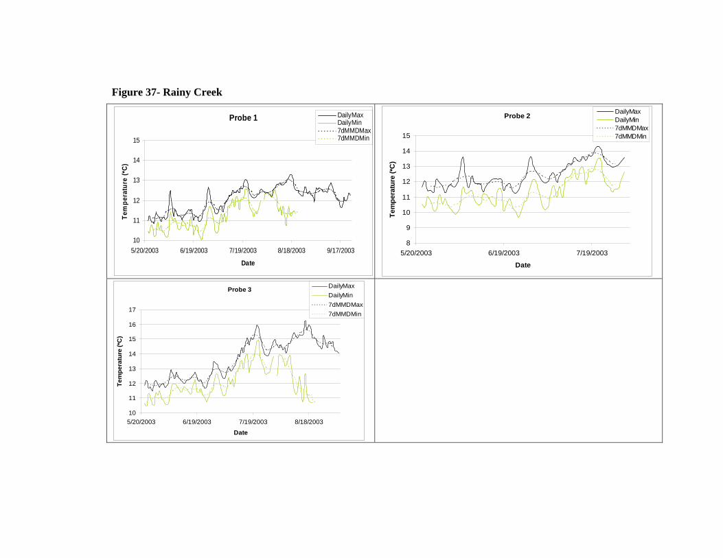
Figure 37- Rainy Creek
Probe 1
10
11
12
13
14
15
5/20/2003 6/19/2003 7/19/2003 8/18/2003 9/17/2003
Date
Tem
pera
ture
(*C)
DailyMaxDailyMin7dMMDMax7dMMDMin
Probe 2
8
9
10
11
12
13
14
15
5/20/2003 6/19/2003 7/19/2003
Date
Tem
pera
ture
(*C
)
DailyMaxDailyMin7dMMDMax7dMMDMin
Probe 3
10
11
12
13
14
15
16
17
5/20/2003 6/19/2003 7/19/2003 8/18/2003
Date
Tem
pera
ture
(*C
)
DailyMaxDailyMin7dMMDMax7dMMDMin
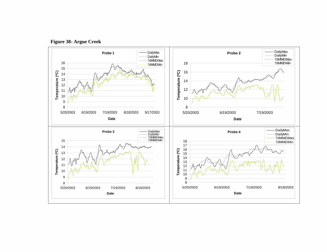
Figure 38- Argue Creek
Probe 1
89
10111213141516
5/20/2003 6/19/2003 7/19/2003 8/18/2003 9/17/2003
Date
Tem
pera
ture
(*C
)DailyMaxDailyMin7dMMDMax7dMMDMin
Probe 2
8
10
12
14
16
18
5/20/2003 6/19/2003 7/19/2003
Date
Tem
pera
ture
(*C
)
DailyMaxDailyMin7dMMDMax7dMMDMin
Probe 3
8
9
10
11
12
13
14
15
5/20/2003 6/19/2003 7/19/2003 8/18/2003
Date
Tem
pera
ture
(*C
)
DailyMaxDailyMin7dMMDMax7dMMDMin
Probe 4
89
101112131415161718
5/20/2003 6/19/2003 7/19/2003 8/18/2003
Date
Tem
pera
ture
(*C
)
DailyMaxDailyMin7dMMDMax7dMMDMin

Appendix C Results of Tracer Tests
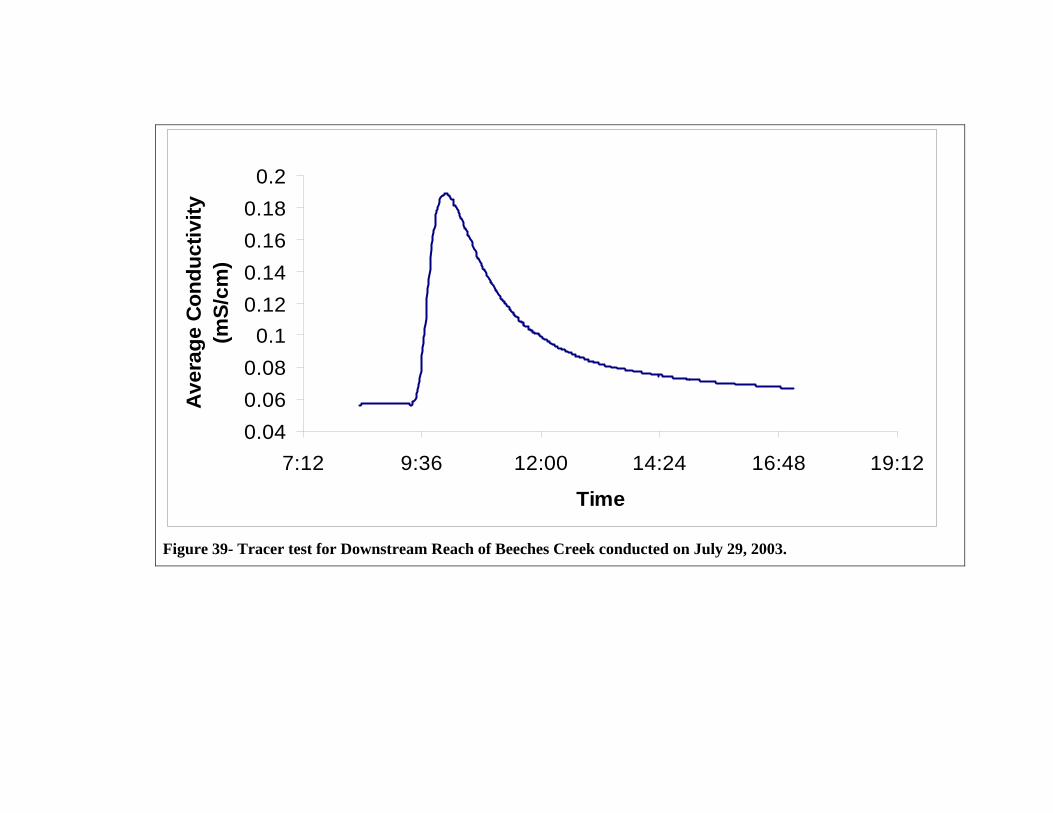
0.040.060.08
0.10.120.140.160.18
0.2
7:12 9:36 12:00 14:24 16:48 19:12
Time
Ave
rage
Con
duct
ivity
(m
S/cm
)
Figure 39- Tracer test for Downstream Reach of Beeches Creek conducted on July 29, 2003.
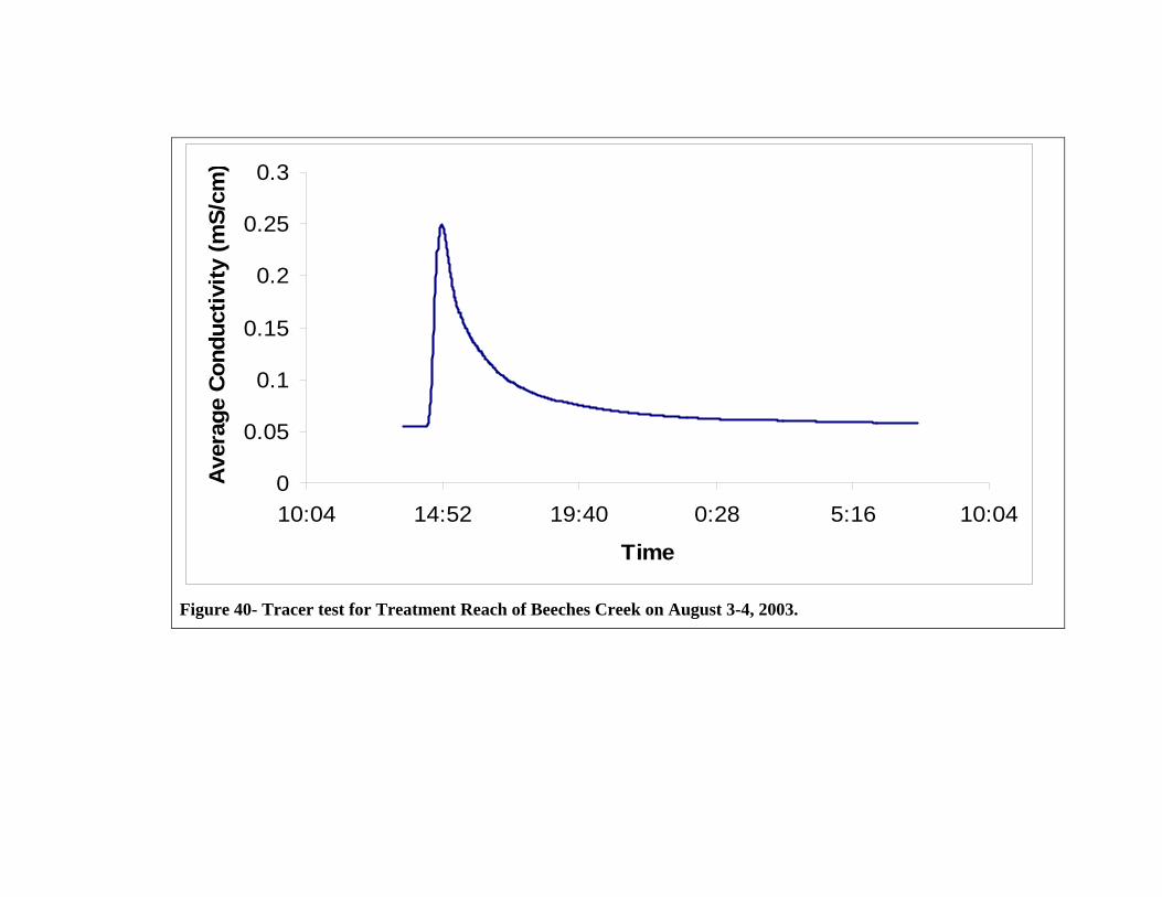
0
0.05
0.1
0.15
0.2
0.25
0.3
10:04 14:52 19:40 0:28 5:16 10:04
Time
Ave
rage
Con
duct
ivity
(mS/
cm)
Figure 40- Tracer test for Treatment Reach of Beeches Creek on August 3-4, 2003.
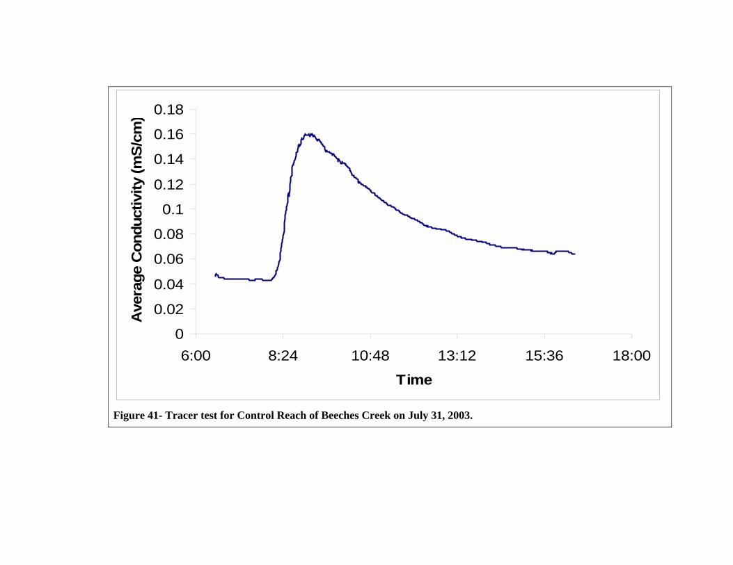
0
0.02
0.04
0.06
0.08
0.1
0.12
0.14
0.16
0.18
6:00 8:24 10:48 13:12 15:36 18:00
Time
Ave
rage
Con
duct
ivity
(mS/
cm)
Figure 41- Tracer test for Control Reach of Beeches Creek on July 31, 2003.
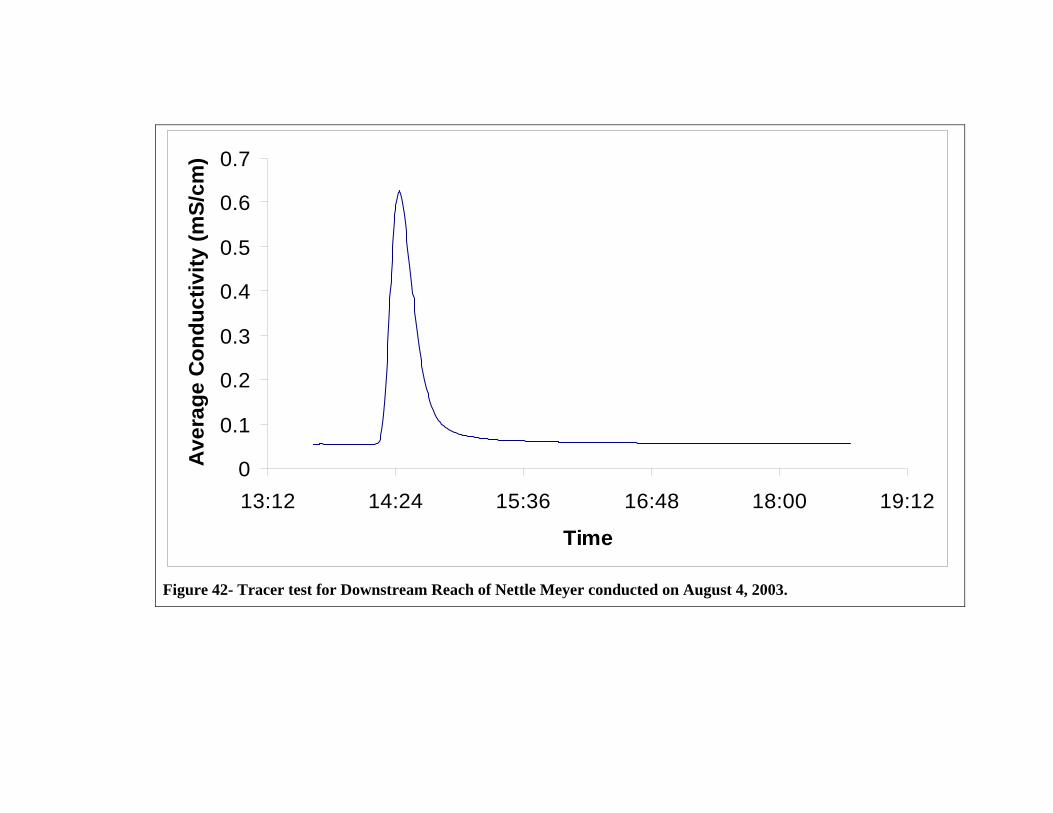
0
0.1
0.2
0.3
0.4
0.5
0.6
0.7
13:12 14:24 15:36 16:48 18:00 19:12
Time
Ave
rage
Con
duct
ivity
(mS/
cm)
Figure 42- Tracer test for Downstream Reach of Nettle Meyer conducted on August 4, 2003.
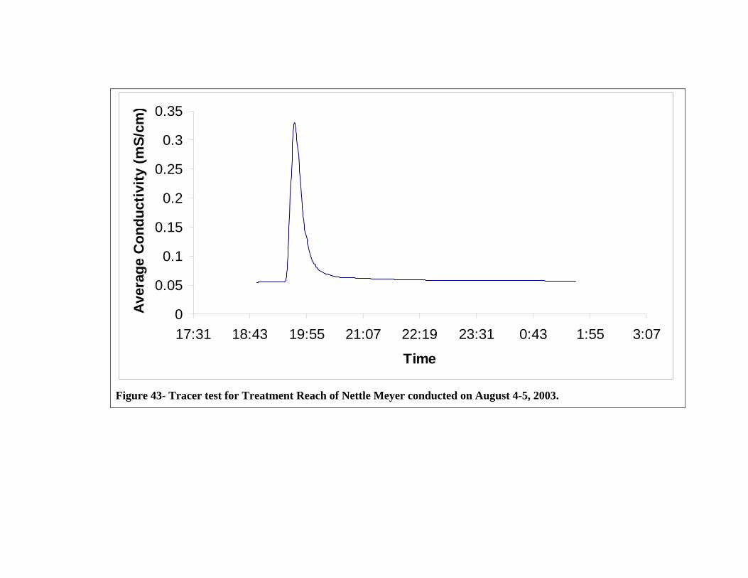
0
0.05
0.1
0.15
0.2
0.25
0.3
0.35
17:31 18:43 19:55 21:07 22:19 23:31 0:43 1:55 3:07
Time
Ave
rage
Con
duct
ivity
(mS/
cm)
Figure 43- Tracer test for Treatment Reach of Nettle Meyer conducted on August 4-5, 2003.

0
0.05
0.1
0.15
0.2
0.25
0.3
0.35
0.4
1:12 2:24 3:36 4:48 6:00 7:12 8:24 9:36
Time
Ave
rage
Con
duct
ivity
(mS/
cm)
Figure 44- Tracer test for Control Reach of Nettle Meyer conducted on August 5, 2003.
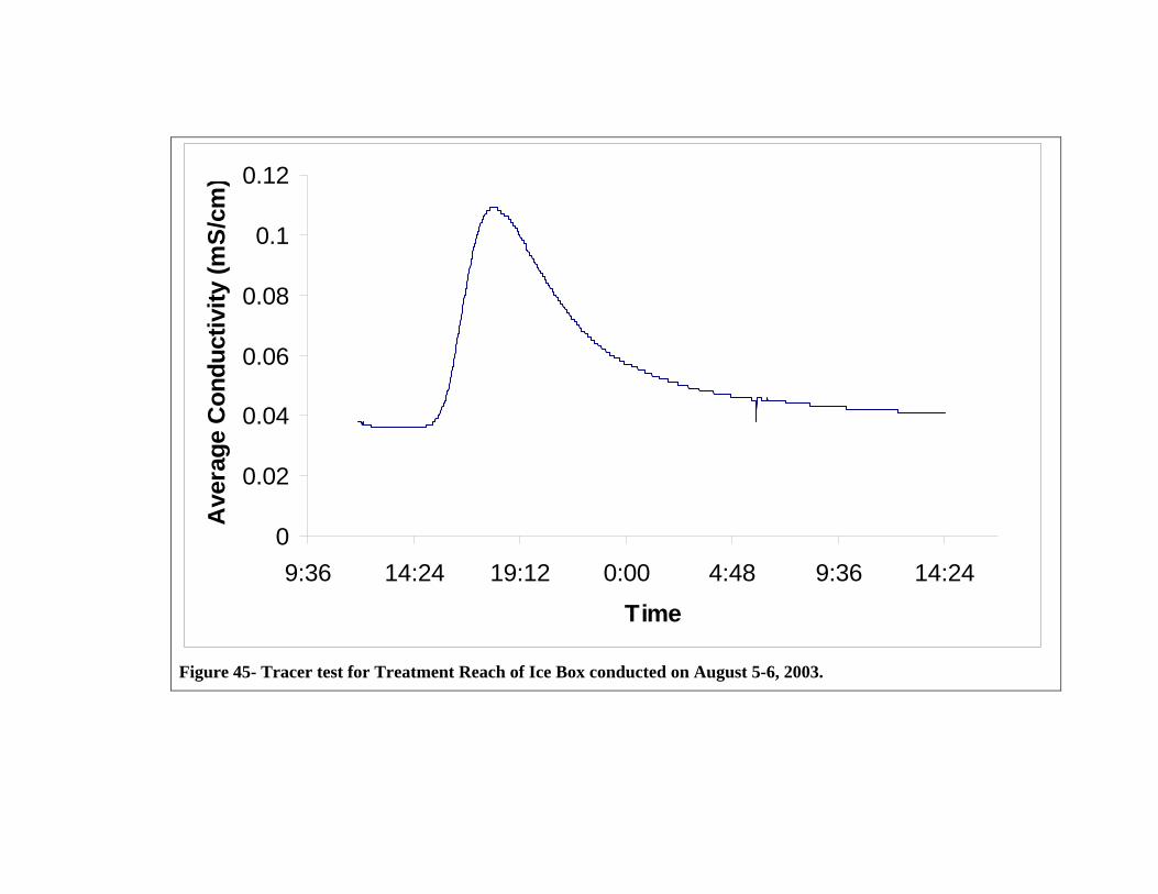
0
0.02
0.04
0.06
0.08
0.1
0.12
9:36 14:24 19:12 0:00 4:48 9:36 14:24
Time
Ave
rage
Con
duct
ivity
(mS/
cm)
Figure 45- Tracer test for Treatment Reach of Ice Box conducted on August 5-6, 2003.
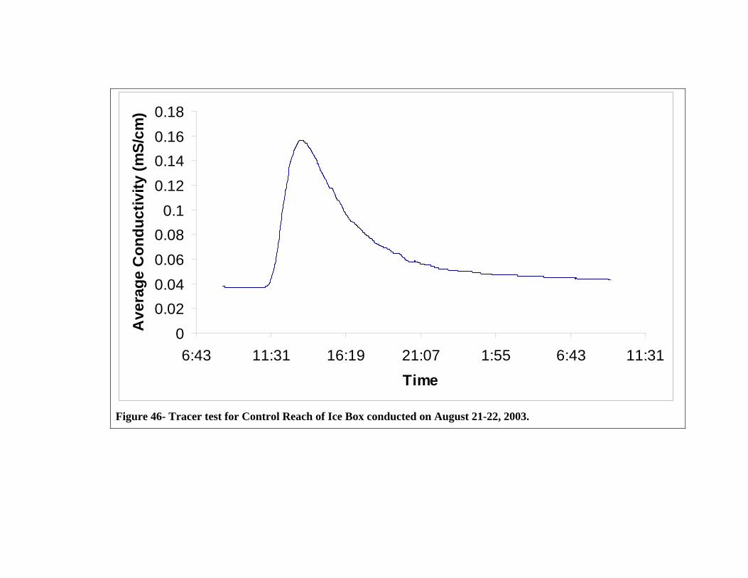
00.020.040.060.08
0.10.120.140.160.18
6:43 11:31 16:19 21:07 1:55 6:43 11:31Time
Ave
rage
Con
duct
ivity
(mS/
cm)
Figure 46- Tracer test for Control Reach of Ice Box conducted on August 21-22, 2003.
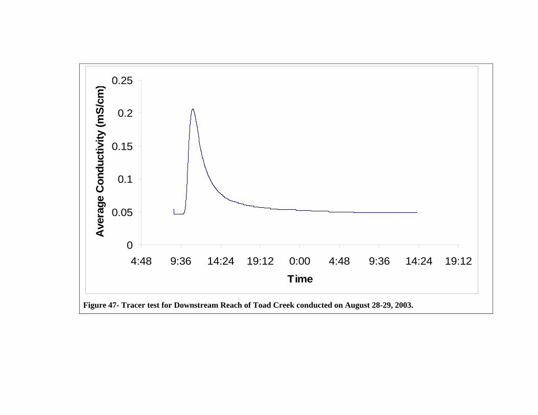
0
0.05
0.1
0.15
0.2
0.25
4:48 9:36 14:24 19:12 0:00 4:48 9:36 14:24 19:12
Time
Ave
rage
Con
duct
ivity
(mS/
cm)
Figure 47- Tracer test for Downstream Reach of Toad Creek conducted on August 28-29, 2003.
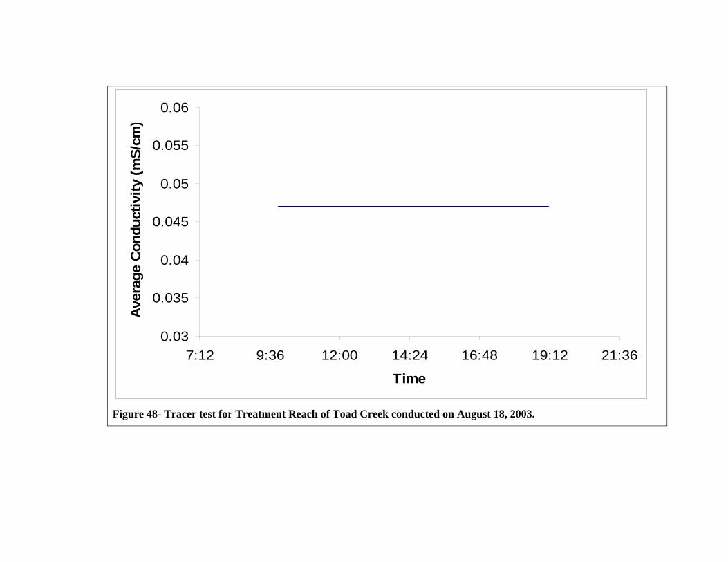
0.03
0.035
0.04
0.045
0.05
0.055
0.06
7:12 9:36 12:00 14:24 16:48 19:12 21:36
Time
Ave
rage
Con
duct
ivity
(mS/
cm)
Figure 48- Tracer test for Treatment Reach of Toad Creek conducted on August 18, 2003.
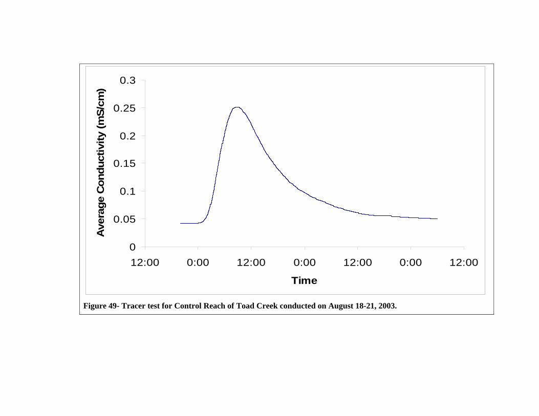
0
0.05
0.1
0.15
0.2
0.25
0.3
12:00 0:00 12:00 0:00 12:00 0:00 12:00
Time
Ave
rage
Con
duct
ivity
(mS/
cm)
Figure 49- Tracer test for Control Reach of Toad Creek conducted on August 18-21, 2003.

Appendix D
Model Combinations by Reach

Control Reach
Table 2- Temperature response variable DiffMax7d in the Control Reach. CR Significant Model Combinations
Models p-value R2
Variable1 p-value R2 1 0.0132 0.2581GeoID 0.0181 0.1724 GeoID 0.0428Region 0.5958 0.0095 Canopy 0.0774BFW 0.7536 0.0033 2 0.0052 0.3044Gradient 0.7501 0.0034 GeoID 0.0015BB 0.0500 0.1220 Region 0.0260Cobble 0.4916 0.0159 3 0.0099 0.2728Gravel 0.8567 0.0011 BB 0.0306Fine 0.1885 0.0569 Canopy 0.0205FPW 0.3777 0.0260 4 0.0178 0.2425Canopy 0.0326 0.1433 Canopy 0.0097small-low 0.6502 0.0069 small-up 0.0611med-low 0.4589 0.0184 5 0.0138 0.2558large-low 0.7918 0.0024 Canopy 0.0121small-up 0.2607 0.0420 wjam# 0.0451med-up 0.8856 0.0007 6 0.0036 0.3791large-up 0.8720 0.0009 Canopy 0.0020wjam# 0.1377 0.0720 small-up 0.0255wjamVol 0.4578 0.0185 wjam# 0.0193
7 0.0042 0.3716Canopy 0.0050small-up 0.0450BB 0.0233
DiffMax7d
1 GeoID = parent geology of streams: sedimentary or basalt; Region = either North Coast, Central Coast, or South Coast; Stream Type = small or medium, fish or non-fish bearing stream; Aspect = directional flow of stream; BFW = bankfull width of
stream; Gradient = steepness of stream channel; BB = substrate combination boulder/bedrock; Cobble, Gravel, and Fine = substrate classifications; Canopy =
percent canopy cover over stream; small-low = small wood volume below height of BFW; med-low = medium wood volume below height of BFW; large-low = large
wood volume below height of BFW; small-up = small wood volume between height of BFW and 1.8m; med-up = medium volume of wood between height of BFW and 1.8m; large-up = large volume of wood between height of BFW and 1.8m; wjam# =
number of wood jams in stream; wjamVol = volume of wood jams in stream.
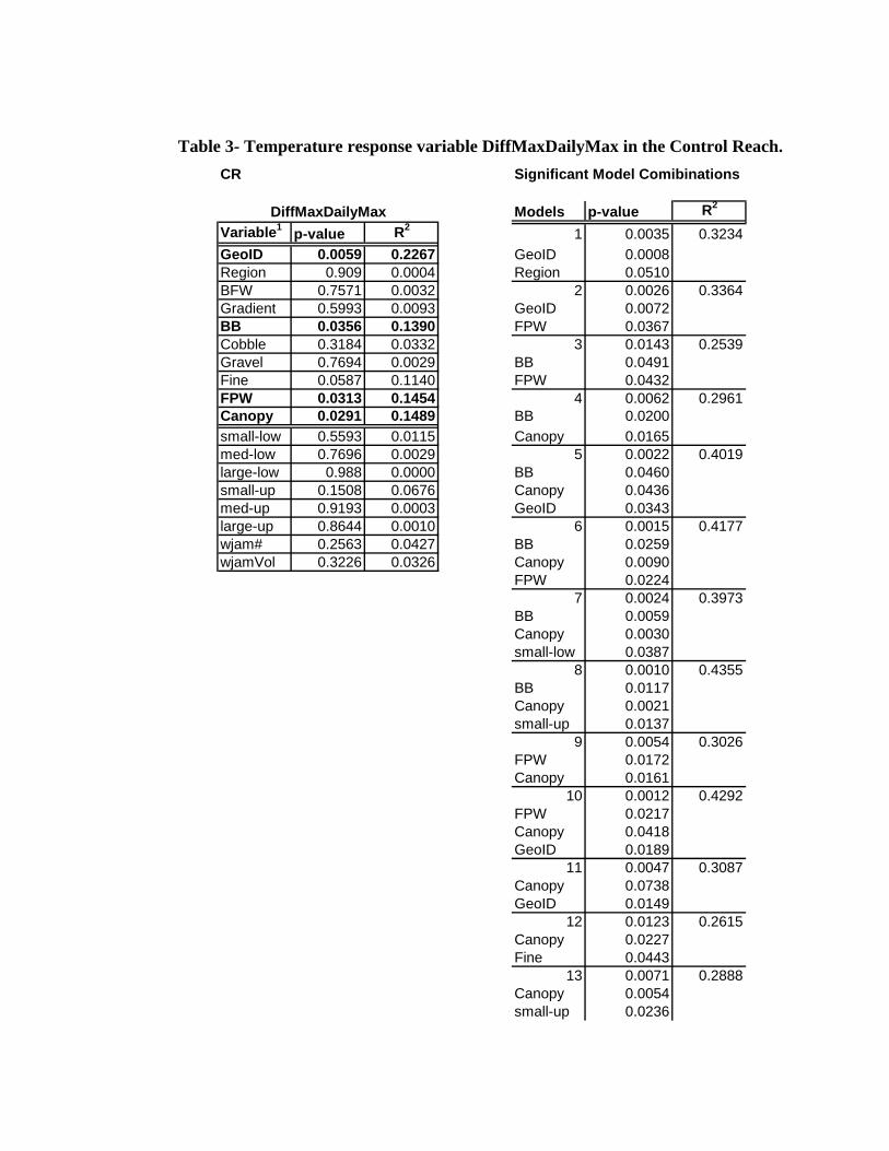
Table 3- Temperature response variable DiffMaxDailyMax in the Control Reach. CR Significant Model Comibinations
Models p-value R2
Variable1 p-value R2 1 0.0035 0.3234GeoID 0.0059 0.2267 GeoID 0.0008Region 0.909 0.0004 Region 0.0510BFW 0.7571 0.0032 2 0.0026 0.3364Gradient 0.5993 0.0093 GeoID 0.0072BB 0.0356 0.1390 FPW 0.0367Cobble 0.3184 0.0332 3 0.0143 0.2539Gravel 0.7694 0.0029 BB 0.0491Fine 0.0587 0.1140 FPW 0.0432FPW 0.0313 0.1454 4 0.0062 0.2961Canopy 0.0291 0.1489 BB 0.0200small-low 0.5593 0.0115 Canopy 0.0165med-low 0.7696 0.0029 5 0.0022 0.4019large-low 0.988 0.0000 BB 0.0460small-up 0.1508 0.0676 Canopy 0.0436med-up 0.9193 0.0003 GeoID 0.0343large-up 0.8644 0.0010 6 0.0015 0.4177wjam# 0.2563 0.0427 BB 0.0259wjamVol 0.3226 0.0326 Canopy 0.0090
FPW 0.02247 0.0024 0.3973
BB 0.0059Canopy 0.0030small-low 0.0387
8 0.0010 0.4355BB 0.0117Canopy 0.0021small-up 0.0137
9 0.0054 0.3026FPW 0.0172Canopy 0.0161
10 0.0012 0.4292FPW 0.0217Canopy 0.0418GeoID 0.0189
11 0.0047 0.3087Canopy 0.0738GeoID 0.0149
12 0.0123 0.2615Canopy 0.0227Fine 0.0443
13 0.0071 0.2888Canopy 0.0054small-up 0.0236
DiffMaxDailyMax

Table 4- Temperature response variable DiffAveMax7d in the Control Reach.
CR Significant Model Combinations
Models p-value R2
Variable1 p-value R2 1 0.0031 0.3289GeoID 0.0044 0.2401 GeoID 0.0060Region 0.7877 0.0025 small-up 0.0598BFW 0.8556 0.0011 2 0.0078 0.2845Gradient 0.2998 0.0358 small-up 0.0081BB 0.2928 0.0368 Canopy 0.0167Cobble 0.7431 0.0036 3 0.0017 0.4124Gravel 0.5735 0.0107 small-up 0.0162Fine 0.2593 0.0422 Canopy 0.0558FPW 0.1825 0.0585 GeoID 0.0199Canopy 0.1046 0.0854 4 0.0014 0.4203small-low 0.0919 0.0918 small-up 0.0023med-low 0.7562 0.0033 Canopy 0.0034large-low 0.5355 0.0129 wjam# 0.0161small-up 0.0467 0.1254med-up 0.3591 0.0281large-up 0.9647 0.0001wjam# 0.1381 0.0718wjamVol 0.8625 0.0010
DiffAve7dMax
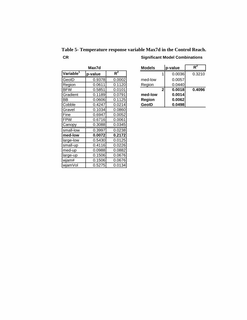
Table 5- Temperature response variable Max7d in the Control Reach. CR Significant Model Combinations
Models p-value R2
Variable1 p-value R2 1 0.0036 0.3210GeoID 0.9378 0.0002 med-low 0.0057Region 0.0611 0.1120 Region 0.0440BFW 0.5851 0.0101 2 0.0018 0.4096Gradient 0.1189 0.0791 med-low 0.0014BB 0.0606 0.1125 Region 0.0062Cobble 0.4247 0.0214 GeoID 0.0498Gravel 0.1034 0.0860Fine 0.6947 0.0052FPW 0.6716 0.0061Canopy 0.3088 0.0345small-low 0.3997 0.0238med-low 0.0072 0.2172large-low 0.5430 0.0125small-up 0.4116 0.0226med-up 0.0988 0.0882large-up 0.1506 0.0676wjam# 0.1506 0.0676wjamVol 0.5275 0.0134
Max7d
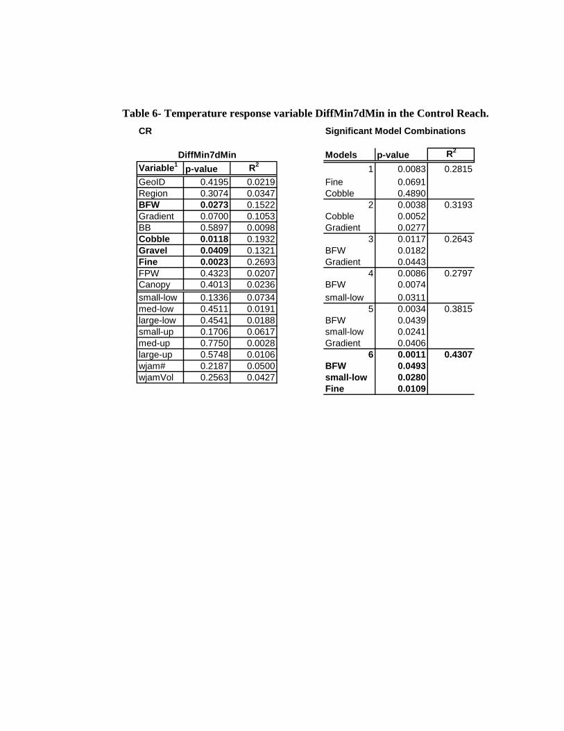
Table 6- Temperature response variable DiffMin7dMin in the Control Reach.
CR Significant Model Combinations
Models p-value R2
Variable1 p-value R2 1 0.0083 0.2815GeoID 0.4195 0.0219 Fine 0.0691Region 0.3074 0.0347 Cobble 0.4890BFW 0.0273 0.1522 2 0.0038 0.3193Gradient 0.0700 0.1053 Cobble 0.0052BB 0.5897 0.0098 Gradient 0.0277Cobble 0.0118 0.1932 3 0.0117 0.2643Gravel 0.0409 0.1321 BFW 0.0182Fine 0.0023 0.2693 Gradient 0.0443FPW 0.4323 0.0207 4 0.0086 0.2797Canopy 0.4013 0.0236 BFW 0.0074small-low 0.1336 0.0734 small-low 0.0311med-low 0.4511 0.0191 5 0.0034 0.3815large-low 0.4541 0.0188 BFW 0.0439small-up 0.1706 0.0617 small-low 0.0241med-up 0.7750 0.0028 Gradient 0.0406large-up 0.5748 0.0106 6 0.0011 0.4307wjam# 0.2187 0.0500 BFW 0.0493wjamVol 0.2563 0.0427 small-low 0.0280
Fine 0.0109
DiffMin7dMin
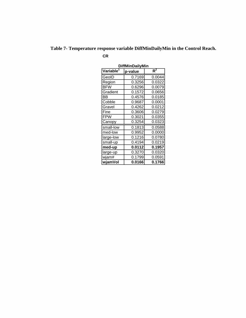
Table 7- Temperature response variable DiffMinDailyMin in the Control Reach. CR
Variable1 p-value R2
GeoID 0.7169 0.0044Region 0.3256 0.0322BFW 0.6296 0.0079Gradient 0.1572 0.0656BB 0.4576 0.0185Cobble 0.9687 0.0001Gravel 0.4262 0.0212Fine 0.3606 0.0279FPW 0.3021 0.0355Canopy 0.3254 0.0323small-low 0.1813 0.0588med-low 0.9952 0.0000large-low 0.1216 0.0780small-up 0.4194 0.0219med-up 0.0112 0.1957large-up 0.3270 0.0320wjam# 0.1799 0.0591wjamVol 0.0166 0.1766
DiffMinDailyMin
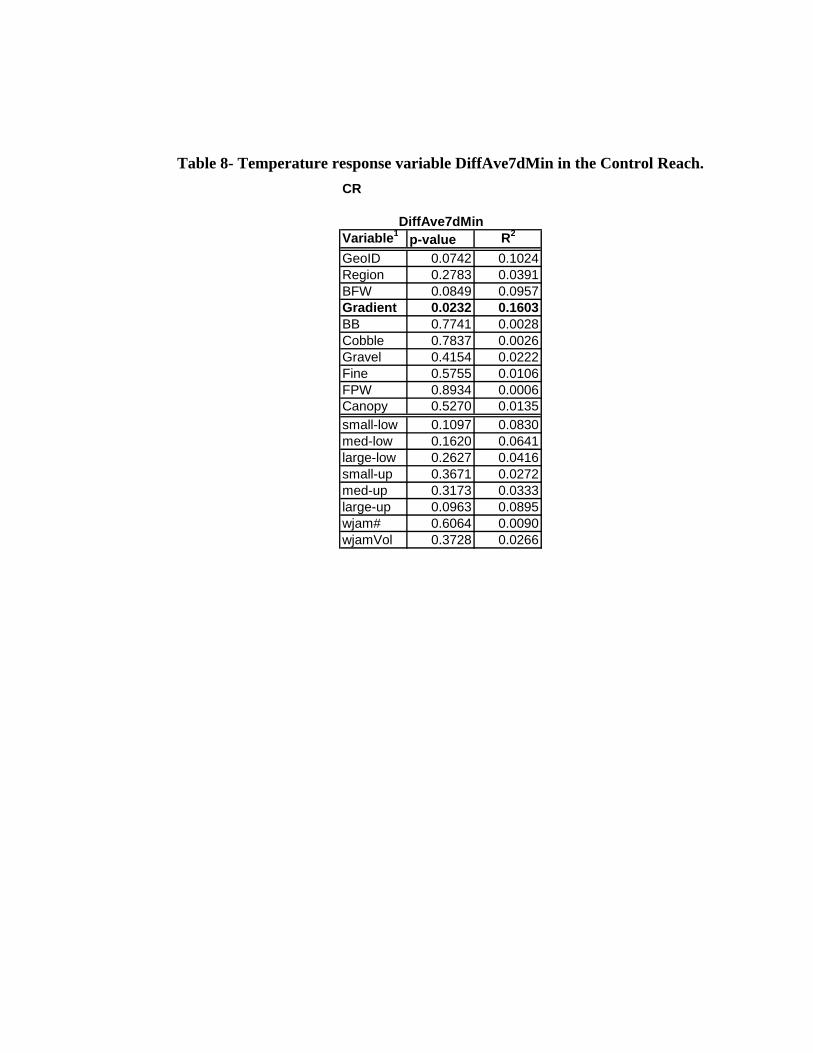
Table 8- Temperature response variable DiffAve7dMin in the Control Reach.
CR
Variable1 p-value R2
GeoID 0.0742 0.1024Region 0.2783 0.0391BFW 0.0849 0.0957Gradient 0.0232 0.1603BB 0.7741 0.0028Cobble 0.7837 0.0026Gravel 0.4154 0.0222Fine 0.5755 0.0106FPW 0.8934 0.0006Canopy 0.5270 0.0135small-low 0.1097 0.0830med-low 0.1620 0.0641large-low 0.2627 0.0416small-up 0.3671 0.0272med-up 0.3173 0.0333large-up 0.0963 0.0895wjam# 0.6064 0.0090wjamVol 0.3728 0.0266
DiffAve7dMin
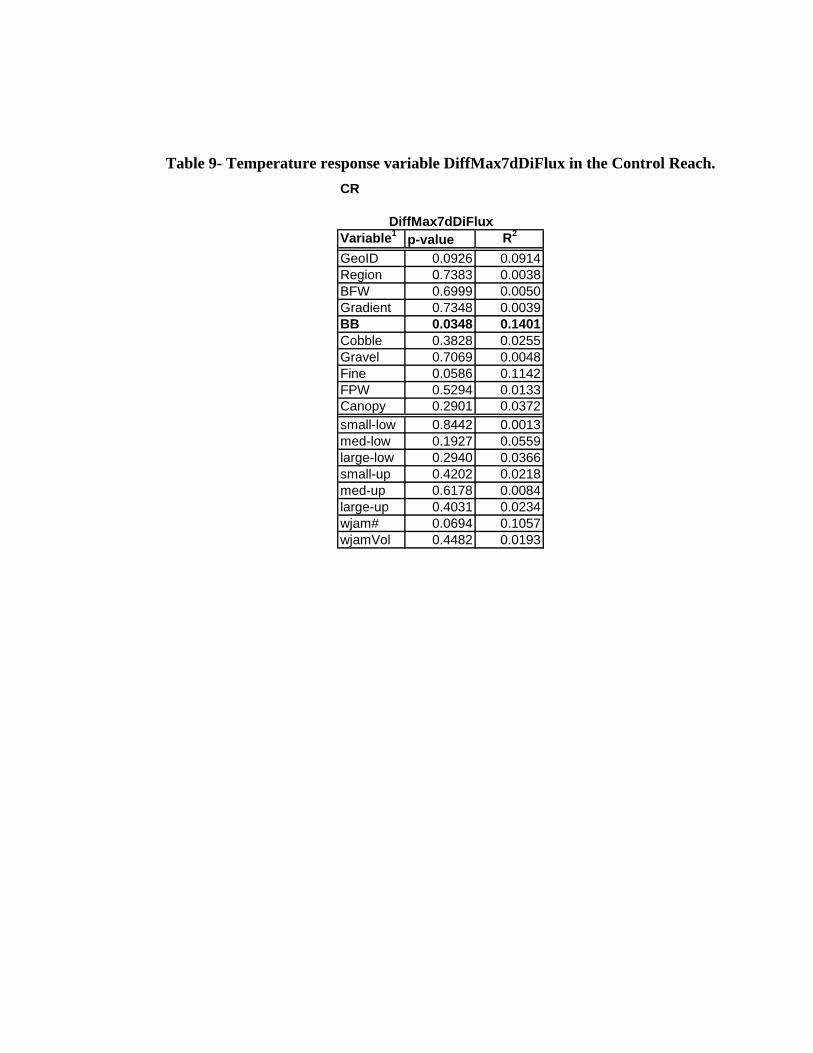
Table 9- Temperature response variable DiffMax7dDiFlux in the Control Reach.
CR
Variable1 p-value R2
GeoID 0.0926 0.0914Region 0.7383 0.0038BFW 0.6999 0.0050Gradient 0.7348 0.0039BB 0.0348 0.1401Cobble 0.3828 0.0255Gravel 0.7069 0.0048Fine 0.0586 0.1142FPW 0.5294 0.0133Canopy 0.2901 0.0372small-low 0.8442 0.0013med-low 0.1927 0.0559large-low 0.2940 0.0366small-up 0.4202 0.0218med-up 0.6178 0.0084large-up 0.4031 0.0234wjam# 0.0694 0.1057wjamVol 0.4482 0.0193
DiffMax7dDiFlux
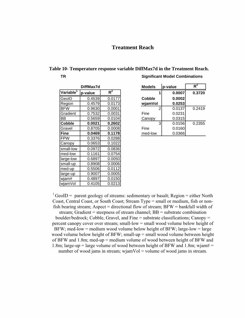
Treatment Reach
Table 10- Temperature response variable DiffMax7d in the Treatment Reach. TR Significant Model Combinations
Models p-value R2
Variable1 p-value R2 1 0.0007 0.3720GeoID 0.4539 0.0177 Cobble 0.0002Region 0.4579 0.0173 wjamVol 0.0253BFW 0.9630 0.0001 2 0.0137 0.2419Gradient 0.7532 0.0031 Fine 0.0231BB 0.5659 0.0104 Canopy 0.0315Cobble 0.0021 0.2602 3 0.0156 0.2355Gravel 0.8705 0.0008 Fine 0.0160Fine 0.0469 0.1178 med-low 0.0366FPW 0.3376 0.0288Canopy 0.0653 0.1022small-low 0.0972 0.0836med-low 0.1161 0.0754large-low 0.6897 0.0050small-up 0.8908 0.0006med-up 0.5506 0.0112large-up 0.9007 0.0005wjam# 0.4897 0.0150wjamVol 0.4105 0.0213
DiffMax7d
1 GeoID = parent geology of streams: sedimentary or basalt; Region = either North Coast, Central Coast, or South Coast; Stream Type = small or medium, fish or non-fish bearing stream; Aspect = directional flow of stream; BFW = bankfull width of
stream; Gradient = steepness of stream channel; BB = substrate combination boulder/bedrock; Cobble, Gravel, and Fine = substrate classifications; Canopy =
percent canopy cover over stream; small-low = small wood volume below height of BFW; med-low = medium wood volume below height of BFW; large-low = large
wood volume below height of BFW; small-up = small wood volume between height of BFW and 1.8m; med-up = medium volume of wood between height of BFW and 1.8m; large-up = large volume of wood between height of BFW and 1.8m; wjam# =
number of wood jams in stream; wjamVol = volume of wood jams in stream.
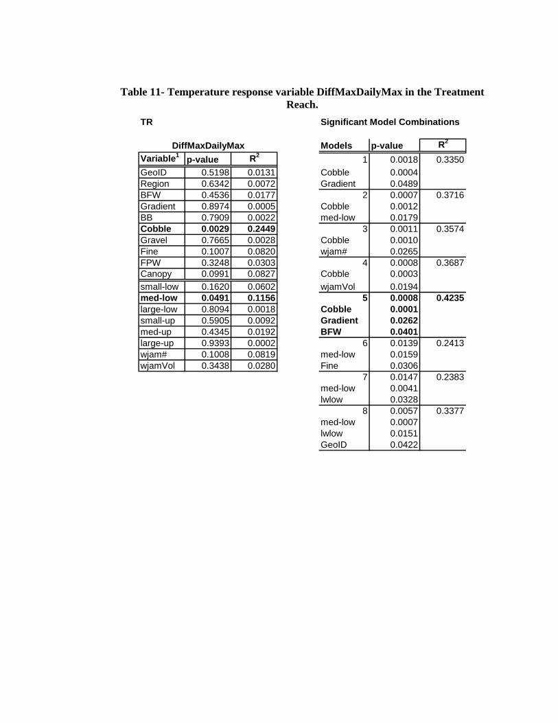
Table 11- Temperature response variable DiffMaxDailyMax in the Treatment Reach.
TR Significant Model Combinations
Models p-value R2
Variable1 p-value R2 1 0.0018 0.3350GeoID 0.5198 0.0131 Cobble 0.0004Region 0.6342 0.0072 Gradient 0.0489BFW 0.4536 0.0177 2 0.0007 0.3716Gradient 0.8974 0.0005 Cobble 0.0012BB 0.7909 0.0022 med-low 0.0179Cobble 0.0029 0.2449 3 0.0011 0.3574Gravel 0.7665 0.0028 Cobble 0.0010Fine 0.1007 0.0820 wjam# 0.0265FPW 0.3248 0.0303 4 0.0008 0.3687Canopy 0.0991 0.0827 Cobble 0.0003small-low 0.1620 0.0602 wjamVol 0.0194med-low 0.0491 0.1156 5 0.0008 0.4235large-low 0.8094 0.0018 Cobble 0.0001small-up 0.5905 0.0092 Gradient 0.0262med-up 0.4345 0.0192 BFW 0.0401large-up 0.9393 0.0002 6 0.0139 0.2413wjam# 0.1008 0.0819 med-low 0.0159wjamVol 0.3438 0.0280 Fine 0.0306
7 0.0147 0.2383med-low 0.0041lwlow 0.0328
8 0.0057 0.3377med-low 0.0007lwlow 0.0151GeoID 0.0422
DiffMaxDailyMax
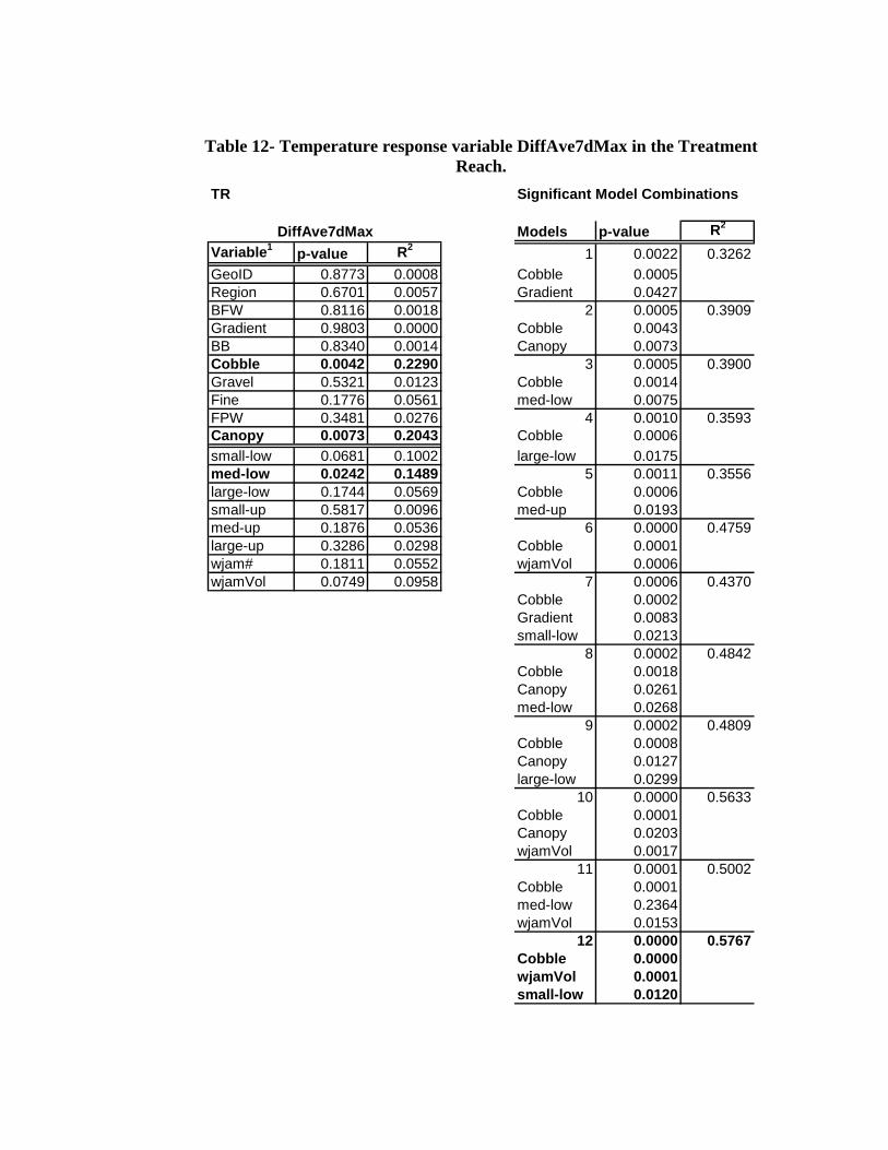
Table 12- Temperature response variable DiffAve7dMax in the Treatment Reach.
TR Significant Model Combinations
Models p-value R2
Variable1 p-value R2 1 0.0022 0.3262GeoID 0.8773 0.0008 Cobble 0.0005Region 0.6701 0.0057 Gradient 0.0427BFW 0.8116 0.0018 2 0.0005 0.3909Gradient 0.9803 0.0000 Cobble 0.0043BB 0.8340 0.0014 Canopy 0.0073Cobble 0.0042 0.2290 3 0.0005 0.3900Gravel 0.5321 0.0123 Cobble 0.0014Fine 0.1776 0.0561 med-low 0.0075FPW 0.3481 0.0276 4 0.0010 0.3593Canopy 0.0073 0.2043 Cobble 0.0006small-low 0.0681 0.1002 large-low 0.0175med-low 0.0242 0.1489 5 0.0011 0.3556large-low 0.1744 0.0569 Cobble 0.0006small-up 0.5817 0.0096 med-up 0.0193med-up 0.1876 0.0536 6 0.0000 0.4759large-up 0.3286 0.0298 Cobble 0.0001wjam# 0.1811 0.0552 wjamVol 0.0006wjamVol 0.0749 0.0958 7 0.0006 0.4370
Cobble 0.0002Gradient 0.0083small-low 0.0213
8 0.0002 0.4842Cobble 0.0018Canopy 0.0261med-low 0.0268
9 0.0002 0.4809Cobble 0.0008Canopy 0.0127large-low 0.0299
10 0.0000 0.5633Cobble 0.0001Canopy 0.0203wjamVol 0.0017
11 0.0001 0.5002Cobble 0.0001med-low 0.2364wjamVol 0.0153
12 0.0000 0.5767Cobble 0.0000wjamVol 0.0001small-low 0.0120
DiffAve7dMax
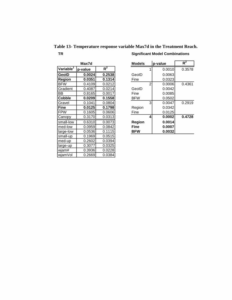
Table 13- Temperature response variable Max7d in the Treatment Reach.
TR Significant Model Combinations
Models p-value R2
Variable1 p-value R2 1 0.0010 0.3578GeoID 0.0024 0.2538 GeoID 0.0063Region 0.0351 0.1314 Fine 0.0323BFW 0.4109 0.0212 2 0.0006 0.4361Gradient 0.4087 0.0214 GeoID 0.0042BB 0.8165 0.0017 Fine 0.0085Cobble 0.0209 0.1558 BFW 0.0502Gravel 0.1041 0.0804 3 0.0047 0.2919Fine 0.0125 0.1798 Region 0.0342FPW 0.1605 0.0606 Fine 0.0125Canopy 0.3170 0.0313 4 0.0002 0.4728small-low 0.6310 0.0073 Region 0.0014med-low 0.0959 0.0842 Fine 0.0007large-low 0.0536 0.1115 BFW 0.0032small-up 0.1969 0.0515med-up 0.2602 0.0394large-up 0.3077 0.0325wjam# 0.3936 0.0228wjamVol 0.2669 0.0384
Max7d

Table 14- Temperature response variable DiffMin7dMin in the Treatment
Reach. TR Significant Model Combinations
Models p-value R2
Variable1 p-value R2 1 0.0083 0.2657GeoID 0.8270 0.0015 Cobble 0.0054Region 0.1888 0.0533 Region 0.0520BFW 0.6806 0.0054 2 0.0049 0.2906Gradient 0.7204 0.0041 Cobble 0.0013BB 0.5418 0.0117 Gradient 0.0280Cobble 0.0157 0.1690Gravel 0.8596 0.0010Fine 0.2769 0.0368FPW 0.7398 0.0035Canopy 0.8028 0.0020small-low 0.9954 0.0000med-low 0.7012 0.0047large-low 0.8846 0.0007small-up 0.5756 0.0099med-up 0.6288 0.0074large-up 0.8109 0.0018wjam# 0.6839 0.0052wjamVol 0.8545 0.0011
DiffMin7dMin
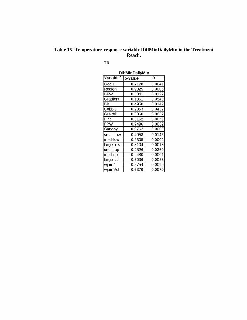
Table 15- Temperature response variable DiffMinDailyMin in the Treatment
Reach. TR
Variable1 p-value R2
GeoID 0.7178 0.0041Region 0.9025 0.0005BFW 0.5341 0.0122Gradient 0.1861 0.0540BB 0.4950 0.0147Cobble 0.2353 0.0437Gravel 0.6860 0.0052Fine 0.6162 0.0079FPW 0.7496 0.0032Canopy 0.9762 0.0000small-low 0.4958 0.0146med-low 0.9305 0.0002large-low 0.8104 0.0018small-up 0.2826 0.0360med-up 0.9480 0.0001large-up 0.6036 0.0085wjam# 0.5754 0.0099wjamVol 0.6379 0.0070
DiffMinDailyMin
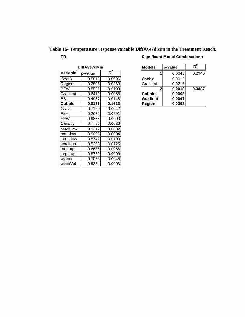
Table 16- Temperature response variable DiffAve7dMin in the Treatment Reach.
TR Significant Model Combinations
Models p-value R2
Variable1 p-value R2 1 0.0045 0.2946GeoID 0.5816 0.0096 Cobble 0.0012Region 0.2805 0.0363 Gradient 0.0215BFW 0.5591 0.0108 2 0.0018 0.3887Gradient 0.6419 0.0068 Cobble 0.0003BB 0.4937 0.0148 Gradient 0.0097Cobble 0.0186 0.1613 Region 0.0398Gravel 0.7169 0.0042Fine 0.2625 0.0391FPW 0.9833 0.0000Canopy 0.7736 0.0026small-low 0.9312 0.0002med-low 0.9098 0.0004large-low 0.5742 0.0100small-up 0.5293 0.0125med-up 0.6685 0.0058large-up 0.8760 0.0008wjam# 0.7073 0.0045wjamVol 0.9284 0.0003
DiffAve7dMin

Table 17- Temperature response variable DiffMax7dDiFlux in the Treatment Reach.
TR
Variable1 p-value R2
GeoID 0.0736 0.0966Region 0.2982 0.0338BFW 0.5201 0.0130Gradient 0.7751 0.0026BB 0.1894 0.0532Cobble 0.2759 0.0370Gravel 0.9957 0.0000Fine 0.1499 0.0637FPW 0.3318 0.0294Shade 0.3137 0.0317small-low 0.3979 0.0224med-low 0.5036 0.0141large-low 0.8961 0.0005small-up 0.9254 0.0003med-up 0.9500 0.0001large-up 0.8915 0.0006wjam# 0.4634 0.0169wjamVol 0.6744 0.0056
DiffMax7dDiFlux

Downstream Reach
Table 18- Temperature response variable DiffMax7d in the Downstream Reach. DR Significant Model Combinations
DiffMax7d Models p-value R2
Variable1 p-value R2 1 0.0186 0.3922GeoID 0.8074 0.0036 med-up 0.0158Region 0.3909 0.0436 BFW 0.0436BFW 0.1542 0.1157Gradient 0.0302 0.2474BB 0.2648 0.0725Cobble 0.5876 0.0177Gravel 0.2682 0.0716Fine 0.7839 0.0045FPW 0.6962 0.0092Canopy 0.9921 0.0000small-low 0.2455 0.0785med-low 0.0763 0.1732large-low 0.0026 0.4213 *small-up 0.2652 0.0724med-up 0.0486 0.2098large-up 0.0214 0.2743wjam# 0.7921 0.0042wjamVol 0.1751 0.1054
1 GeoID = parent geology of streams: sedimentary or basalt; Region = either North Coast, Central Coast, or South Coast; Stream Type = small or medium, fish or non-fish bearing stream; Aspect = directional flow of stream; BFW = bankfull width of
stream; Gradient = steepness of stream channel; BB = substrate combination boulder/bedrock; Cobble, Gravel, and Fine = substrate classifications; Canopy =
percent canopy cover over stream; small-low = small wood volume below height of BFW; med-low = medium wood volume below height of BFW; large-low = large
wood volume below height of BFW; small-up = small wood volume between height of BFW and 1.8m; med-up = medium volume of wood between height of BFW and 1.8m; large-up = large volume of wood between height of BFW and 1.8m; wjam# =
number of wood jams in stream; wjamVol = volume of wood jams in stream.

Table 19- Temperature response variable DiffMaxDailyMax in the Downstream Reach.
DR Significant Model Combinations
Models p-value R2
Variable1 p-value R2 1 0.0225 0.3777GeoID 0.5246 0.0242 large-low 0.0067Region 0.7134 0.0081 WjamVol 0.0511BFW 0.3076 0.0611Gradient 0.2415 0.0797BB 0.0765 0.1730Cobble 0.4957 0.0277Gravel 0.2219 0.0864Fine 0.4184 0.0389FPW 0.3222 0.0576Caonpy 0.6924 0.0094small-low 0.2502 0.0770med-low 0.2022 0.0938large-low 0.0517 0.2049small-up 0.7586 0.0057med-up 0.5193 0.0248large-up 0.0684 0.1822wjam# 0.9307 0.0005wjamVol 0.8966 0.0010
DiffMaxDailyMax
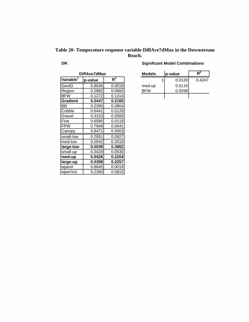
Table 20- Temperature response variable DiffAve7dMax in the Downstream
Reach. DR Significant Model Combinations
Models p-value R2
Variable1 p-value R2 1 0.0120 0.4247GeoID 0.8636 0.0018 med-up 0.0115Region 0.2882 0.0660 BFW 0.0299BFW 0.1272 0.1314Gradient 0.0447 0.2165BB 0.2395 0.0804Cobble 0.6441 0.0128Gravel 0.3153 0.0593Fine 0.6580 0.0118FPW 0.7948 0.0041Canopy 0.9471 0.0003small-low 0.2051 0.0927med-low 0.0542 0.2010large-low 0.0039 0.3962small-up 0.3429 0.0530med-up 0.0426 0.2204large-up 0.0398 0.2257wjam# 0.8645 0.0018wjamVol 0.2360 0.0815
DiffAve7dMax
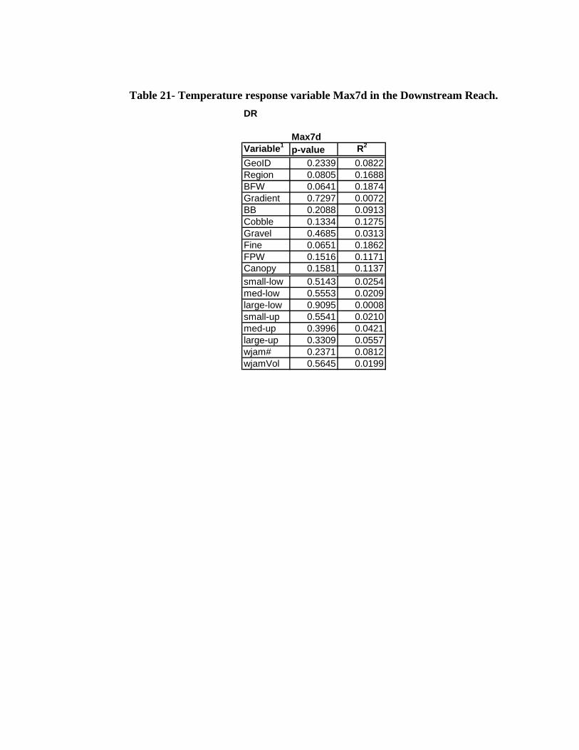
Table 21- Temperature response variable Max7d in the Downstream Reach. DR
Max7dVariable1 p-value R2
GeoID 0.2339 0.0822Region 0.0805 0.1688BFW 0.0641 0.1874Gradient 0.7297 0.0072BB 0.2088 0.0913Cobble 0.1334 0.1275Gravel 0.4685 0.0313Fine 0.0651 0.1862FPW 0.1516 0.1171Canopy 0.1581 0.1137small-low 0.5143 0.0254med-low 0.5553 0.0209large-low 0.9095 0.0008small-up 0.5541 0.0210med-up 0.3996 0.0421large-up 0.3309 0.0557wjam# 0.2371 0.0812wjamVol 0.5645 0.0199

Table 22- Temperature response variable DiffMin7dMin in the Downstream Reach.
DR
Variable1 p-value R2
GeoID 0.8374 0.0025Region 0.6835 0.0100BFW 0.8368 0.0026Gradient 0.6945 0.0093BB 0.5776 0.0186Cobble 0.5622 0.0201Gravel 0.6982 0.0091Fine 0.4738 0.0306FPW 0.1492 0.1184Canopy 0.3619 0.0491small-low 0.9320 0.0004med-low 0.4726 0.0308large-low 0.7851 0.0045small-up 0.4369 0.0360med-up 0.2958 0.0641large-up 0.7039 0.0087wjam# 0.9590 0.0002wjamVol 0.9187 0.0006
DiffMin7dMin

Table 23- Temperature response variable DiffMinDailyMin in the Downstream Reach.
DR
Variable1 p-value R2
GeoID 0.0792 0.1702Region 0.1751 0.1054BFW 0.1907 0.0985Gradient 0.3277 0.0564BB 0.2321 0.0828Cobble 0.0599 0.1930Gravel 0.8136 0.0034Fine 0.8609 0.0019FPW 0.4556 0.0332Canopy 0.4339 0.0364small-low 0.1862 0.1004med-low 0.8517 0.0021large-low 0.5191 0.0249small-up 0.2199 0.0871med-up 0.4936 0.0280large-up 0.2275 0.0844wjam# 0.2007 0.0944wjamVol 0.1958 0.0964
DiffMinDailyMin
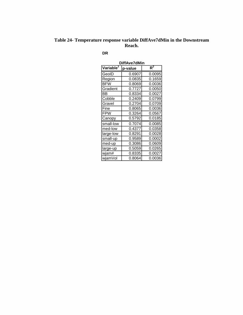
Table 24- Temperature response variable DiffAve7dMin in the Downstream Reach.
DR
Variable1 p-value R2
GeoID 0.6907 0.0095Region 0.0835 0.1659BFW 0.8069 0.0036Gradient 0.7727 0.0050BB 0.8334 0.0027Cobble 0.2409 0.0799Gravel 0.2704 0.0709Fine 0.8065 0.0036FPW 0.3264 0.0567Canopy 0.5792 0.0185small-low 0.7074 0.0085med-low 0.4377 0.0358large-low 0.8291 0.0028small-up 0.9589 0.0002med-up 0.3086 0.0609large-up 0.5059 0.0265wjam# 0.8335 0.0027wjamVol 0.8064 0.0036
DiffAve7dMin

Table 25- Temperature response variable DiffMax7dDiFlux in the Downstream Reach.
DR
Variable1 p-value R2
GeoID 0.8762 0.0015Region 0.8630 0.0018BFW 0.0957 0.1547Gradient 0.0757 0.1739BB 0.2953 0.0642Cobble 0.3999 0.0420Gravel 0.7276 0.0073Fine 0.6290 0.0140FPW 0.3629 0.0489Canopy 0.7928 0.0042small-low 0.1107 0.1428med-low 0.1838 0.1015large-low 0.0159 0.2968small-up 0.1530 0.1163med-up 0.2289 0.0839large-up 0.0237 0.2664wjam# 0.8634 0.0018wjamVol 0.3738 0.0468
DiffMax7dDiFlux
Recommended