2016/12/03 CV勉強会@関東ECCV2016読み会 発表資料
2016/12/03@peisuke
自己紹介
名前:藤本 敬介
研究:ロボティクス、コンピュータビジョン
点群:形状統合、メッシュ化、認識
画像:画像認識、SfM・MVSロボット:自律移動、動作計画
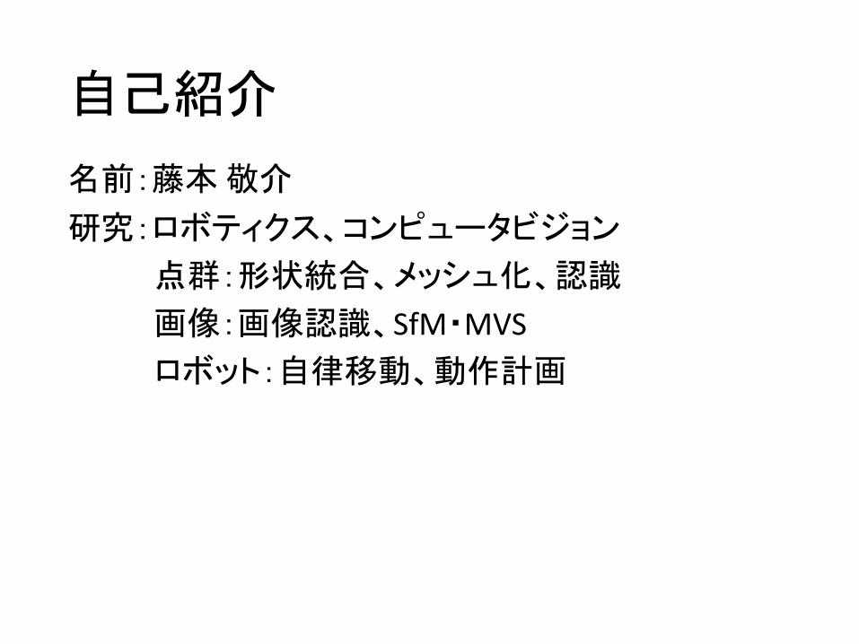
本発表の概要
• 発表論文• Sublabel-AccurateConvexRelaxationofVectorialMultilabelEnergies
• どんな論文?• 多次元のラベリング問題を凸緩和によって効率良く解く
• ノイズ除去、密オプティカルフロー、ステレオマッチング等
• 特徴は?• 問題を複数の区間に分け、区間ごとに凸関数で近似
• 一般的な式に対する解法なので汎用性高
※資料が間に合わなかったので、後で挙げ直します
Sublabel-AccurateConvexRelaxationofVectorialMultilabelEnergies
EmanuelLaude,ThomasMöllenhoff,MichaelMoeller,JanLellmann,DanielCremers
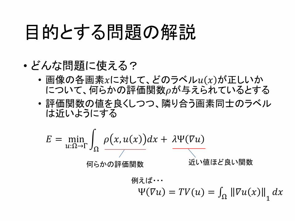
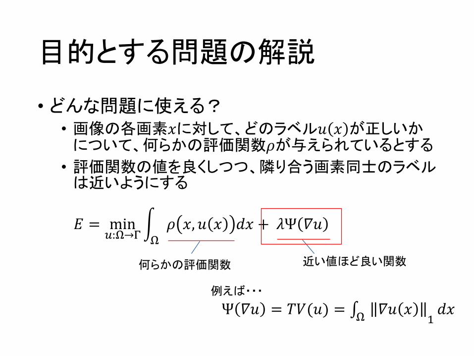
目的とする問題の解説
• どんな問題に使える?• 画像の各画素𝑥に対して、どのラベル𝑢 𝑥 が正しいか
について、何らかの評価関数𝜌が与えられているとする
• 評価関数の値を良くしつつ、隣り合う画素同士のラベルは近いようにする
𝐸 = min):+→-
. 𝜌 𝑥, 𝑢 𝑥 𝑑𝑥 + 𝜆Ψ 𝛻𝑢+
Ψ 𝛻𝑢 = 𝑇𝑉(𝑢) = ∫ 𝛻𝑢 𝑥+ ;𝑑𝑥
近い値ほど良い関数何らかの評価関数
例えば・・・

目的とする問題の解説
• どんな問題に使える?• 画像の各画素𝑥に対して、どのラベル𝑢 𝑥 が正しいか
について、何らかの評価関数𝜌が与えられているとする
• 評価関数の値を良くしつつ、隣り合う画素同士のラベルは近いようにする
𝐸 = min):+→-
. 𝜌 𝑥, 𝑢 𝑥 𝑑𝑥 + 𝜆Ψ 𝛻𝑢+
Ψ 𝛻𝑢 = 𝑇𝑉(𝑢) = ∫ 𝛻𝑢 𝑥+ ;𝑑𝑥
近い値ほど良い関数何らかの評価関数
例えば・・・
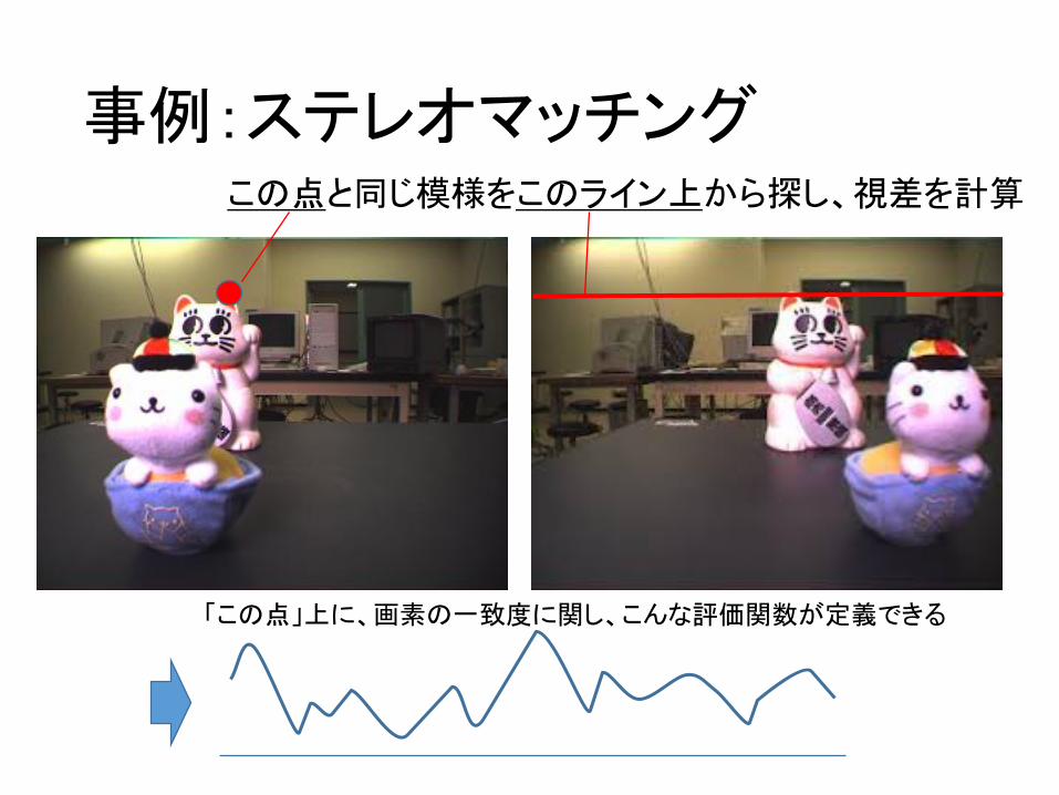
事例:ステレオマッチングこの点と同じ模様をこのライン上から探し、視差を計算
「この点」上に、画素の一致度に関し、こんな評価関数が定義できる
事例:ステレオマッチング
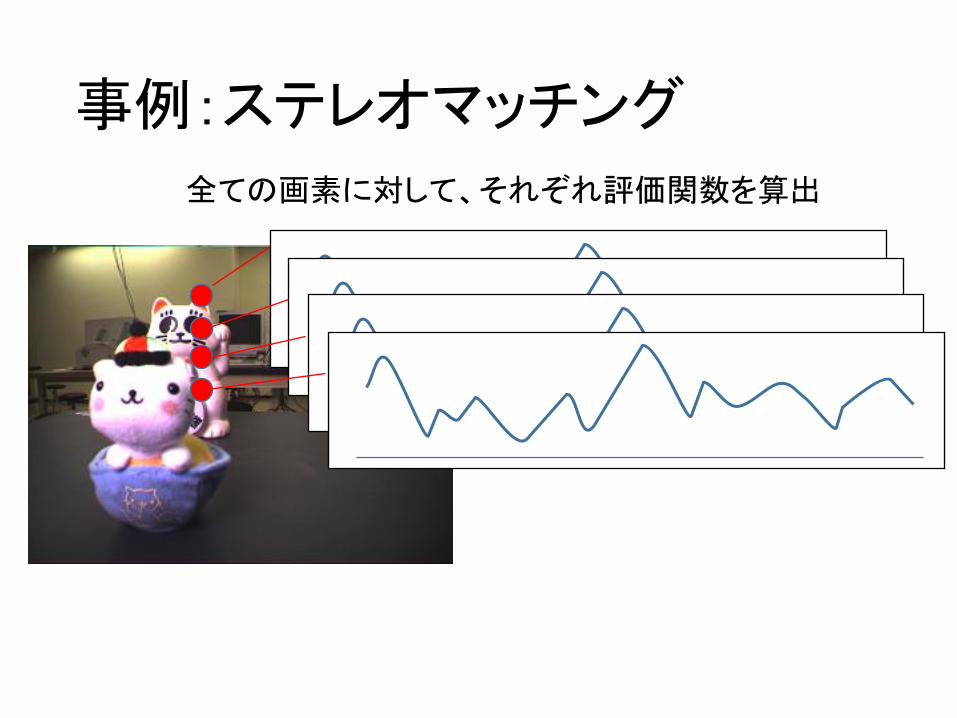
全ての画素に対して、それぞれ評価関数を算出
事例:ステレオマッチング
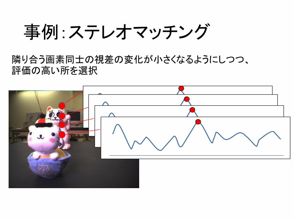
隣り合う画素同士の視差の変化が小さくなるようにしつつ、評価の高い所を選択
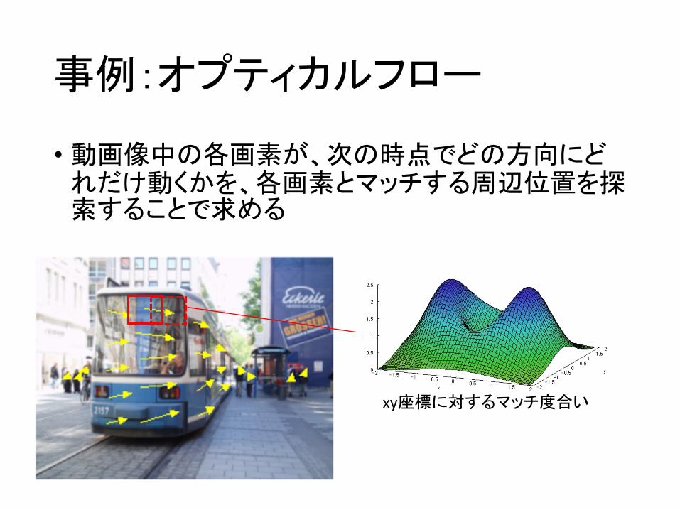
事例:オプティカルフロー
• 動画像中の各画素が、次の時点でどの方向にどれだけ動くかを、各画素とマッチする周辺位置を探索することで求める
xy座標に対するマッチ度合い

事例:オプティカルフロー
• ステレオマッチングと同様に隣り合う画素同士のフローの変化が小さくなるようにしつつ、マッチ度を高くする
目的とする問題の解説
• どんな問題に使える?• 画像の各画素𝑥に対して、どのラベル𝑢 𝑥 が正しいか
について、何らかの評価関数𝜌が与えられているとする
• 評価関数の値を良くしつつ、隣り合う画素同士のラベルは近いようにする
𝐸 = min):+→-
. 𝜌 𝑥, 𝑢 𝑥 𝑑𝑥 + 𝜆Ψ 𝛻𝑢+
Ψ 𝛻𝑢 = 𝑇𝑉(𝑢) = ∫ 𝛻𝑢 𝑥+ ;𝑑𝑥
近い値ほど良い関数何らかの評価関数
例えば・・・
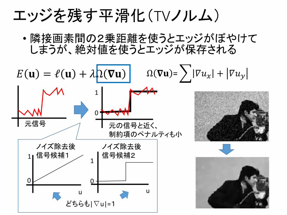
エッジを残す平滑化(TVノルム)
• 隣接画素間の2乗距離を使うとエッジがぼやけてしまうが、絶対値を使うとエッジが保存される
𝐸 𝐮 = ℓ 𝐮 + 𝜆Ω 𝛁𝐮 Ω 𝛁𝐮 =@ 𝛻𝑢A + 𝛻𝑢B
�
�
uu
0
1
0
1
どちらも|∇u|=1
0
1
元の信号と近く、制約項のペナルティも小
元信号
ノイズ除去後信号候補1
ノイズ除去後信号候補2
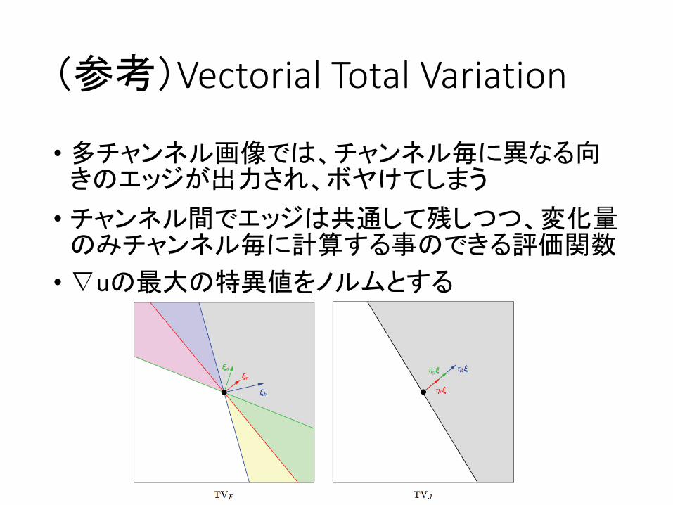
(参考)VectorialTotalVariation
• 多チャンネル画像では、チャンネル毎に異なる向きのエッジが出力され、ボヤけてしまう
• チャンネル間でエッジは共通して残しつつ、変化量のみチャンネル毎に計算する事のできる評価関数
•∇uの最大の特異値をノルムとする
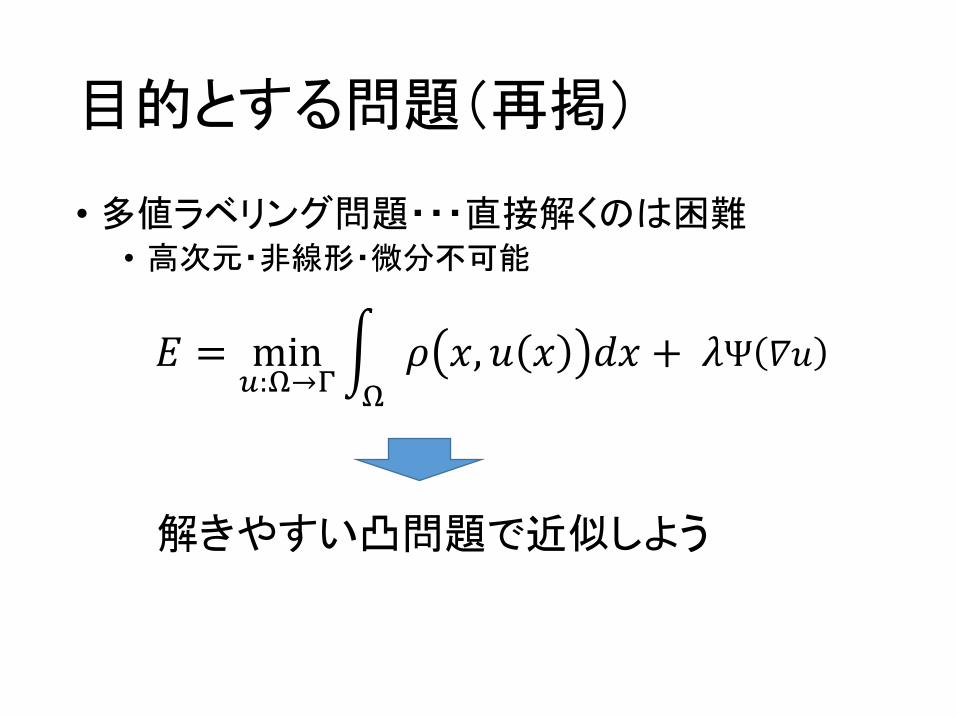
目的とする問題(再掲)
• 多値ラベリング問題・・・直接解くのは困難• 高次元・非線形・微分不可能
𝐸 = min):+→-
. 𝜌 𝑥, 𝑢 𝑥 𝑑𝑥 + 𝜆Ψ 𝛻𝑢+
解きやすい凸問題で近似しよう
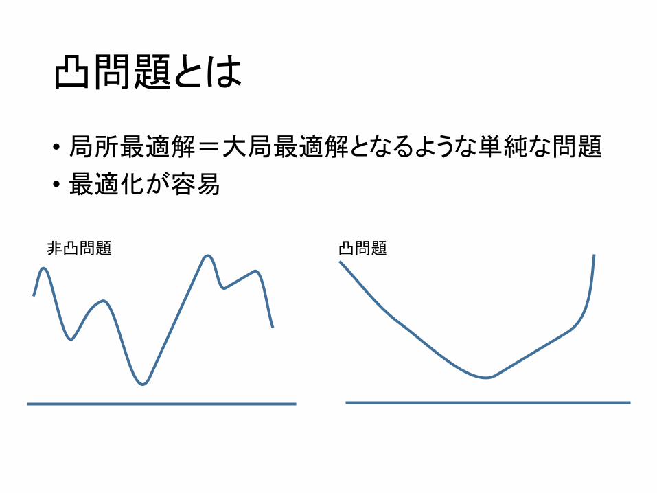
凸問題とは
• 局所最適解=大局最適解となるような単純な問題
• 最適化が容易
非凸問題 凸問題

近似方法について
• 目的関数fの双共役(双対の双対)を取ると、fを下から抑える凸関数f**に変換できる
𝑓 𝒙 𝑓∗∗ 𝒙
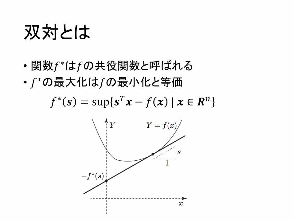
双対とは
• 関数𝑓∗は𝑓の共役関数と呼ばれる
• 𝑓∗の最大化は𝑓の最小化と等価
𝑓∗ 𝒔 = sup 𝒔K𝒙 − 𝑓 𝒙 |𝒙 ∈ 𝑹P
Sublabel-Accurate Convex Relaxation of
Vectorial Multilabel Energies
Emanuel Laude?1, Thomas Mollenho↵?1, Michael Moeller1,
Jan Lellmann2, and Daniel Cremers1
1Technical University of Munich?? 2University of Lubeck
Abstract. Convex relaxations of multilabel problems have been demon-
strated to produce provably optimal or near-optimal solutions to a va-
riety of computer vision problems. Yet, they are of limited practical use
as they require a fine discretization of the label space, entailing a huge
demand in memory and runtime. In this work, we propose the first sub-
label accurate convex relaxation for vectorial multilabel problems. Our
key idea is to approximate the dataterm in a piecewise convex (rather
than piecewise linear) manner. As a result we have a more faithful ap-
proximation of the original cost function that provides a meaningful in-
terpretation for fractional solutions of the relaxed convex problem.
Keywords: Convex Relaxation, Optimization, Variational Methods
(a) Original dataterm (b) Without lifting (c) Classical lifting (d) Proposed lifting
Fig. 1: In (a) we show a nonconvex dataterm. Convexification without lifting
would result in the energy (b). Classical lifting methods [11] (c), approximate
the energy piecewise linearly between the labels, whereas the proposed method
results in an approximation that is convex on each triangle (d). Therefore, we
are able to capture the structure of the nonconvex energy much more accurately.
? These authors contributed equally.?? This work was supported by the ERC Starting Grant “Convex Vision”.
arX
iv:1
604.
0198
0v2
[cs.C
V]
10 O
ct 2
016
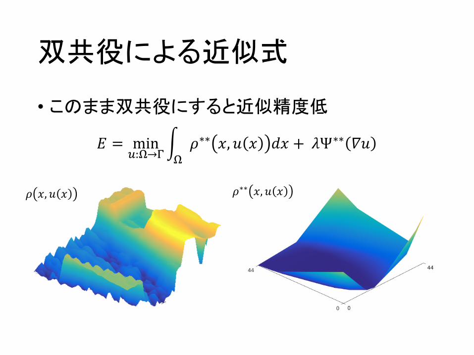
双共役による近似式
• このまま双共役にすると近似精度低
𝐸 = min):+→-
. 𝜌∗∗ 𝑥, 𝑢 𝑥 𝑑𝑥 + 𝜆Ψ∗∗ 𝛻𝑢+
𝜌∗∗ 𝑥, 𝑢 𝑥𝜌 𝑥, 𝑢 𝑥
Sublabel-Accurate Convex Relaxation of
Vectorial Multilabel Energies
Emanuel Laude?1, Thomas Mollenho↵?1, Michael Moeller1,
Jan Lellmann2, and Daniel Cremers1
1Technical University of Munich?? 2University of Lubeck
Abstract. Convex relaxations of multilabel problems have been demon-
strated to produce provably optimal or near-optimal solutions to a va-
riety of computer vision problems. Yet, they are of limited practical use
as they require a fine discretization of the label space, entailing a huge
demand in memory and runtime. In this work, we propose the first sub-
label accurate convex relaxation for vectorial multilabel problems. Our
key idea is to approximate the dataterm in a piecewise convex (rather
than piecewise linear) manner. As a result we have a more faithful ap-
proximation of the original cost function that provides a meaningful in-
terpretation for fractional solutions of the relaxed convex problem.
Keywords: Convex Relaxation, Optimization, Variational Methods
(a) Original dataterm (b) Without lifting (c) Classical lifting (d) Proposed lifting
Fig. 1: In (a) we show a nonconvex dataterm. Convexification without lifting
would result in the energy (b). Classical lifting methods [11] (c), approximate
the energy piecewise linearly between the labels, whereas the proposed method
results in an approximation that is convex on each triangle (d). Therefore, we
are able to capture the structure of the nonconvex energy much more accurately.
? These authors contributed equally.?? This work was supported by the ERC Starting Grant “Convex Vision”.
arX
iv:1
604.
0198
0v2
[cs.C
V]
10 O
ct 2
016
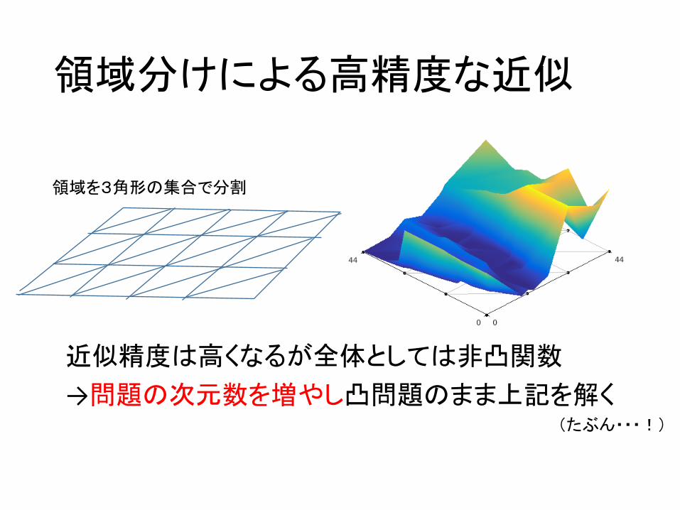
領域分けによる高精度な近似
近似精度は高くなるが全体としては非凸関数
→問題の次元数を増やし凸問題のまま上記を解く
領域を3角形の集合で分割
(たぶん・・・!)

LiftedRepresentation
• 変数を高次元の変数に変換• 変数uを、uの属する3角形の頂点の線形和で表す
• u =(0.3,0.2)→ 0.7*t2+0.1*t3+0.2*t6
• 使わなかった頂点はゼロとして、要素数が頂点数のベクトルに変換• (0,0.7,0.1,0,0,0.2)
Sublabel-Accurate Convex Relaxation of Vectorial Multilabel Energies 5
�1 0 10
1
u(x) = 0.7e2+ 0.1e
3+ 0.2e
6
= (0, 0.7, 0.1, 0, 0, 0.2)>
�1
�4
0.2
0.3
t
6
t
2t
3
Fig. 2: This figure illustrates our notation and the one-to-one correspondence
between u(x) = (0.3, 0.2)> and the lifted u(x) containing the barycentric co-
ordinates ↵ = (0.7, 0.1, 0.2)> of the sublabel u(x) 2 �4 = conv{t2, t3, t6}. Thetriangulation (V, T ) of � = [�1; 1] ⇥ [0; 1] is visualized via the gray lines, cor-
responding to the triangles and the gray dots, corresponding to the vertices
V = {(�1, 0)>, (0, 0)>, . . . , (1, 1)>}, that we refer to as the labels.
2.2 Convexifying the Dataterm
Let for now the weight of the regularizer in (1) be zero. Then, at each point
x 2 ⌦ we minimize a generally nonconvex energy over a compact set � ⇢ Rn:
minu2�
⇢(u). (6)
We set up the lifted energy so that it attains finite values if and only if the
argument u is a sparse representation u = E
i
↵ of a sublabel u 2 � :
⇢(u) = min1i|T |
⇢i
(u), ⇢i
(u) =
8
<
:
⇢(Ti
↵), if u = E
i
↵, ↵ 2 �
U
n
,
1, otherwise.(7)
Problems (6) and (7) are equivalent due to the one-to-one correspondence of
u = T
i
↵ and u = E
i
↵. However, energy (7) is finite on a nonconvex set only. In
order to make optimization tractable, we minimize its convex envelope.
Proposition 1 The convex envelope of (7) is given as:
⇢⇤⇤(u) = supv2R|V|
hu,vi � max1i|T |
⇢⇤i
(v),
⇢⇤i
(v) = hEi
b
i
,vi+ ⇢
⇤i
(A>i
E
>i
v), ⇢
i
:= ⇢+ �
�i .
(8)
b
i
and A
i
are given as b
i
:= M
n+1i
, A
i
:=�
M
1i
, M
2i
, . . . , M
n
i
�
, where M
j
i
are
the columns of the matrix M
i
:= (T>i
,1)�> 2 Rn+1⇥n+1.
Proof. Follows from a calculation starting at the definition of ⇢⇤⇤. See Ap-
pendix A for a detailed derivation.
𝑢 =@𝒖R𝑡R
�
�
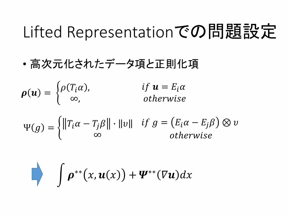
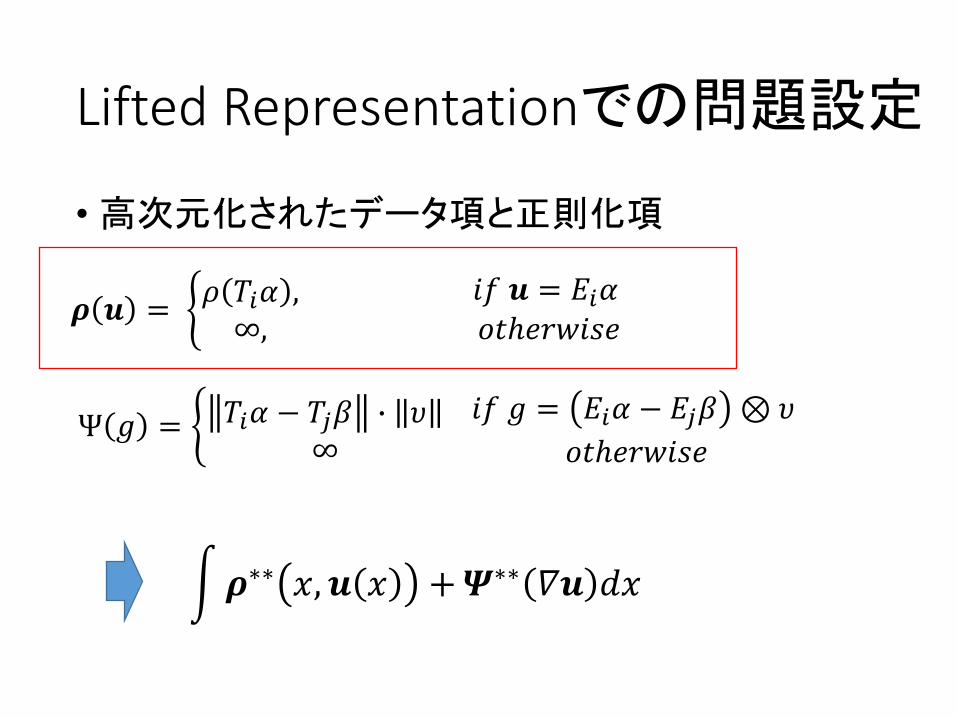
LiftedRepresentationでの問題設定
• 高次元化されたデータ項と正則化項
𝝆 𝒖 = U𝜌 𝑇R𝛼 ,∞,
Ψ 𝑔 = U 𝑇R𝛼 − 𝑇Y𝛽 [ 𝜐∞
𝑖𝑓𝒖 = 𝐸R𝛼𝑜𝑡ℎ𝑒𝑟𝑤𝑖𝑠𝑒
𝑖𝑓𝑔 = 𝐸R𝛼 − 𝐸Y𝛽 ⊗ 𝜐𝑜𝑡ℎ𝑒𝑟𝑤𝑖𝑠𝑒
.𝝆∗∗ 𝑥, 𝒖 𝑥 +�
�
𝜳∗∗ 𝛻𝒖 𝑑𝑥
LiftedRepresentationでの問題設定
• 高次元化されたデータ項と正則化項
𝝆 𝒖 = U𝜌 𝑇R𝛼 ,∞,
Ψ 𝑔 = U 𝑇R𝛼 − 𝑇Y𝛽 [ 𝜐∞
𝑖𝑓𝒖 = 𝐸R𝛼𝑜𝑡ℎ𝑒𝑟𝑤𝑖𝑠𝑒
𝑖𝑓𝑔 = 𝐸R𝛼 − 𝐸Y𝛽 ⊗ 𝜐𝑜𝑡ℎ𝑒𝑟𝑤𝑖𝑠𝑒
.𝝆∗∗ 𝑥, 𝒖 𝑥 +�
�
𝜳∗∗ 𝛻𝒖 𝑑𝑥
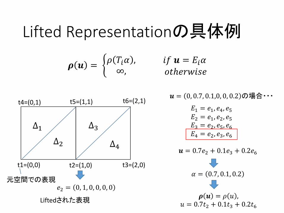
LiftedRepresentationの具体例
𝝆 𝒖 = U𝜌 𝑇R𝛼 ,∞,
𝑖𝑓𝒖 = 𝐸R𝛼𝑜𝑡ℎ𝑒𝑟𝑤𝑖𝑠𝑒
𝒖 = 0, 0.7, 0.1,0, 0, 0.2 の場合・・・
𝐸; = 𝑒;, 𝑒k, 𝑒l𝐸m = 𝑒;, 𝑒m, 𝑒l𝐸n = 𝑒m, 𝑒l, 𝑒o𝐸k = 𝑒m, 𝑒n, 𝑒o
t1=(0,0) t2=(1,0) t3=(2,0)
t4=(0,1) t5=(1,1) t6=(2,1)
∆;∆m
∆n
∆k 𝒖 = 0.7𝑒m + 0.1𝑒n + 0.2𝑒o
𝑒m = 0, 1, 0, 0, 0, 0元空間での表現
Liftedされた表現
𝛼 = 0.7, 0.1, 0.2
𝝆 𝒖 = 𝜌 𝑢 ,𝑢 = 0.7𝑡m + 0.1𝑡n + 0.2𝑡o
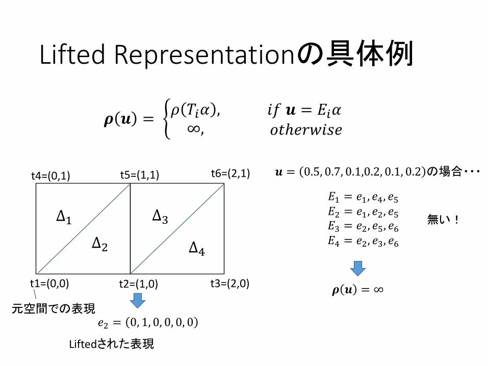
LiftedRepresentationの具体例
𝝆 𝒖 = U𝜌 𝑇R𝛼 ,∞,
𝑖𝑓𝒖 = 𝐸R𝛼𝑜𝑡ℎ𝑒𝑟𝑤𝑖𝑠𝑒
𝒖 = 0.5, 0.7, 0.1,0.2, 0.1, 0.2 の場合・・・
𝐸; = 𝑒;, 𝑒k, 𝑒l𝐸m = 𝑒;, 𝑒m, 𝑒l𝐸n = 𝑒m, 𝑒l, 𝑒o𝐸k = 𝑒m, 𝑒n, 𝑒o
t1=(0,0) t2=(1,0) t3=(2,0)
t4=(0,1) t5=(1,1) t6=(2,1)
∆;∆m
∆n
∆k
𝑒m = 0, 1, 0, 0, 0, 0元空間での表現
Liftedされた表現
𝝆 𝒖 = ∞
無い!

LiftedRepresentationでの問題設定
• 高次元化されたデータ項と正則化項
𝝆 𝒖 = U𝜌 𝑇R𝛼 ,∞,
Ψ 𝑔 = U 𝑇R𝛼 − 𝑇Y𝛽 [ 𝜐∞
𝑖𝑓𝒖 = 𝐸R𝛼𝑜𝑡ℎ𝑒𝑟𝑤𝑖𝑠𝑒
𝑖𝑓𝑔 = 𝐸R𝛼 − 𝐸Y𝛽 ⊗ 𝜐𝑜𝑡ℎ𝑒𝑟𝑤𝑖𝑠𝑒
.𝝆∗∗ 𝑥, 𝒖 𝑥 +�
�
𝜳∗∗ 𝛻𝒖 𝑑𝑥

LiftedRepresentationの具体例
t1=(0,0) t2=(1,0) t3=(2,0)
t4=(0,1) t5=(1,1) t6=(2,1)
∆;
∆k
Ψ 𝑔 = U 𝑇R𝛼 − 𝑇Y𝛽 [ 𝜐∞
𝑖𝑓𝑔 = 𝐸R𝛼 − 𝐸Y𝛽 ⊗ 𝜐𝑜𝑡ℎ𝑒𝑟𝑤𝑖𝑠𝑒
𝑇R𝛼
𝑇Y𝛽 𝜐
画像上のエッジ
※𝜐は正則化項の双対に出てくる補助変数と等価、計算上は陽に出て来ない
[ ; = sup @𝑢Rdiv�
R
𝜂R𝝊 − 𝛿
𝛻𝑢
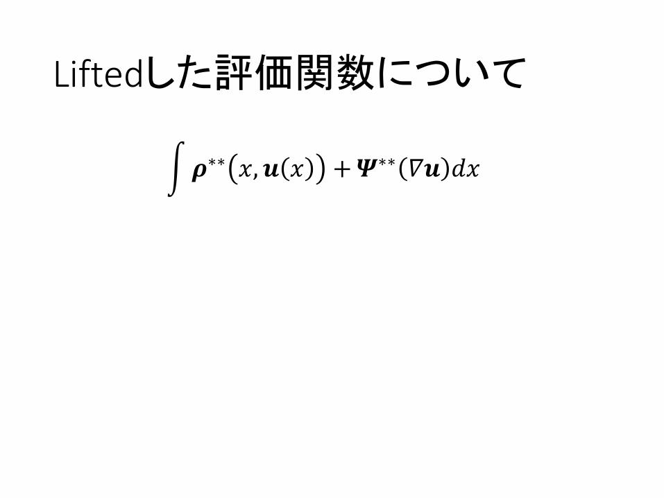
Liftedした評価関数について
.𝝆∗∗ 𝑥, 𝒖 𝑥 +�
�
𝜳∗∗ 𝛻𝒖 𝑑𝑥

Liftedした評価関数について
.𝝆∗∗ 𝑥, 𝒖 𝑥 +�
�
𝜳∗∗ 𝛻𝒖 𝑑𝑥
Sublabel-Accurate Convex Relaxation of Vectorial Multilabel Energies 9
3 Numerical Optimization
3.1 Discretization
For now assume that ⌦ ⇢ Rd is a d-dimensional Cartesian grid and let Div
denote a finite-di↵erence divergence operator with Div q : ⌦ ! R|V|. Then the
relaxed energy minimization problem becomes
minu:⌦!R|V|
maxq:⌦!K
X
x2⌦
⇢⇤⇤(x,u(x)) + hDiv q,ui. (18)
In order to get rid of the pointwise maximum over ⇢⇤i
(v) in Eq. (8), we introduce
additional variables w(x) 2 R and additional constraints (v(x), w(x)) 2 C, x 2 ⌦
so that w(x) attains the value of the pointwise maximum:
minu:⌦!R|V|
max(v,w):⌦!Cq:⌦!K
X
x2⌦
hu(x),v(x)i � w(x) + hDiv q,ui, (19)
where the set C is given as
C =\
1i|T |
Ci
, Ci
:=n
(x, y) 2 R|V|+1 | ⇢⇤i
(x) y
o
. (20)
For numerical optimization we use a GPU-based implementation1 of a first-order
primal-dual method [14]. The algorithm requires the orthogonal projections of
the dual variables onto the sets C respectively K in every iteration. However, the
projection onto an epigraph of dimension |V| + 1 is di�cult for large values of
|V|. We rewrite the constraints (v(x), w(x)) 2 Ci
, 1 i |T |, x 2 ⌦ as (n+ 1)-
dimensional epigraph constraints introducing variables ri(x) 2 Rn, si
(x) 2 R:
⇢
⇤i
�
r
i(x)�
s
i
(x), r
i(x) = A
>i
E
>i
v(x), s
i
(x) = w(x)� hEi
b
i
,v(x)i. (21)
These equality constraints can be implemented using Lagrange multipliers. For
the projection onto the set K we use an approach similar to [7, Figure 7].
3.2 Epigraphical Projections
Computing the Euclidean projection onto the epigraph of ⇢⇤i
is a central part
of the numerical implementation of the presented method. However, for n > 1
this is nontrivial. Therefore we provide a detailed explanation of the projection
methods used for di↵erent classes of ⇢i
. We will consider quadratic, truncated
quadratic and piecewise linear ⇢.
1https://github.com/tum-vision/sublabel_relax
8 E. Laude, T. Mollenho↵, M. Moeller, J. Lellmann, D. Cremers
Proof. Follows from a calculation starting at the definition of the convex conju-
gate ⇤. See Appendix A.
Interestingly, although in its original formulation (14) the set K has infinitely
many constraints, one can equivalently represent K by finitely many.
Proposition 3 The set K in equation (14) is the same as
K =n
q 2 Rd⇥|V| |�
�
D
i
q
�
�
S
1 1, 1 i |T |o
, D
i
q = Q
i
D (Ti
D)�1, (15)
where the matrices Q
i
D 2 Rd⇥n
and T
i
D 2 Rn⇥n
are given as
Q
i
D :=�
qi1 � qin+1, . . . , qin � qin+1
�
, T
i
D :=�
t
i1 � t
in+1, . . . , t
in � t
in+1�
.
Proof. Similar to the analysis in [11], equation (14) basically states the Lipschitz
continuity of a piecewise linear function defined by the matrices q 2 Rd⇥|V|.
Therefore, one can expect that the Lipschitz constraint is equivalent to a bound
on the derivative. For the complete proof, see Appendix A.
2.4 Lifting the Overall Optimization Problem
Combining dataterm and regularizer, the overall optimization problem is given
minu:⌦!R|V|
supq:⌦!K
Z
⌦
⇢⇤⇤(u) + hu,Div qi dx. (16)
A highly desirable property is that, opposed to any other vectorial lifting ap-
proach from the literature, our method with just one simplex applied to a convex
problem yields the same solution as the unlifted problem.
Proposition 4 If the triangulation contains only 1 simplex, T = {�}, i.e.,
|V| = n+ 1, then the proposed optimization problem (16) is equivalent to
minu:⌦!�
Z
⌦
(⇢+ �
�
)⇤⇤(x, u(x)) dx+ �TV (u), (17)
which is (1) with a globally convexified dataterm on �.
Proof. For u = t
n+1+TDu the substitution u =⇣
u1, . . . , un
, 1�P
n
j=1 uj
⌘
into
⇢⇤⇤ and R yields the result. For a complete proof, see Appendix A.
Sublabel-Accurate Convex Relaxation of Vectorial Multilabel Energies 5
�1 0 10
1
u(x) = 0.7e2+ 0.1e
3+ 0.2e
6
= (0, 0.7, 0.1, 0, 0, 0.2)>
�1
�4
0.2
0.3
t
6
t
2t
3
Fig. 2: This figure illustrates our notation and the one-to-one correspondence
between u(x) = (0.3, 0.2)> and the lifted u(x) containing the barycentric co-
ordinates ↵ = (0.7, 0.1, 0.2)> of the sublabel u(x) 2 �4 = conv{t2, t3, t6}. Thetriangulation (V, T ) of � = [�1; 1] ⇥ [0; 1] is visualized via the gray lines, cor-
responding to the triangles and the gray dots, corresponding to the vertices
V = {(�1, 0)>, (0, 0)>, . . . , (1, 1)>}, that we refer to as the labels.
2.2 Convexifying the Dataterm
Let for now the weight of the regularizer in (1) be zero. Then, at each point
x 2 ⌦ we minimize a generally nonconvex energy over a compact set � ⇢ Rn:
minu2�
⇢(u). (6)
We set up the lifted energy so that it attains finite values if and only if the
argument u is a sparse representation u = E
i
↵ of a sublabel u 2 � :
⇢(u) = min1i|T |
⇢i
(u), ⇢i
(u) =
8
<
:
⇢(Ti
↵), if u = E
i
↵, ↵ 2 �
U
n
,
1, otherwise.(7)
Problems (6) and (7) are equivalent due to the one-to-one correspondence of
u = T
i
↵ and u = E
i
↵. However, energy (7) is finite on a nonconvex set only. In
order to make optimization tractable, we minimize its convex envelope.
Proposition 1 The convex envelope of (7) is given as:
⇢⇤⇤(u) = supv2R|V|
hu,vi � max1i|T |
⇢⇤i
(v),
⇢⇤i
(v) = hEi
b
i
,vi+ ⇢
⇤i
(A>i
E
>i
v), ⇢
i
:= ⇢+ �
�i .
(8)
b
i
and A
i
are given as b
i
:= M
n+1i
, A
i
:=�
M
1i
, M
2i
, . . . , M
n
i
�
, where M
j
i
are
the columns of the matrix M
i
:= (T>i
,1)�> 2 Rn+1⇥n+1.
Proof. Follows from a calculation starting at the definition of ⇢⇤⇤. See Ap-
pendix A for a detailed derivation.
一見難しそうに見えるけど・・・

一見難しそうに見えるけど・・・
むずかしい!!

凸問題を解く際の戦略
• 主問題の変数で最適化と双対問題の変数で最適化を交互に繰り返す
• 主問題の変数とは、元々の問題にあった変数
• 双対問題の変数は、後から加えた変数
𝑓∗ 𝒔 = sup 𝒔K𝒙 − 𝑓 𝒙 |𝒙 ∈ 𝑹P𝑓 𝒙双対
sが双対問題の変数
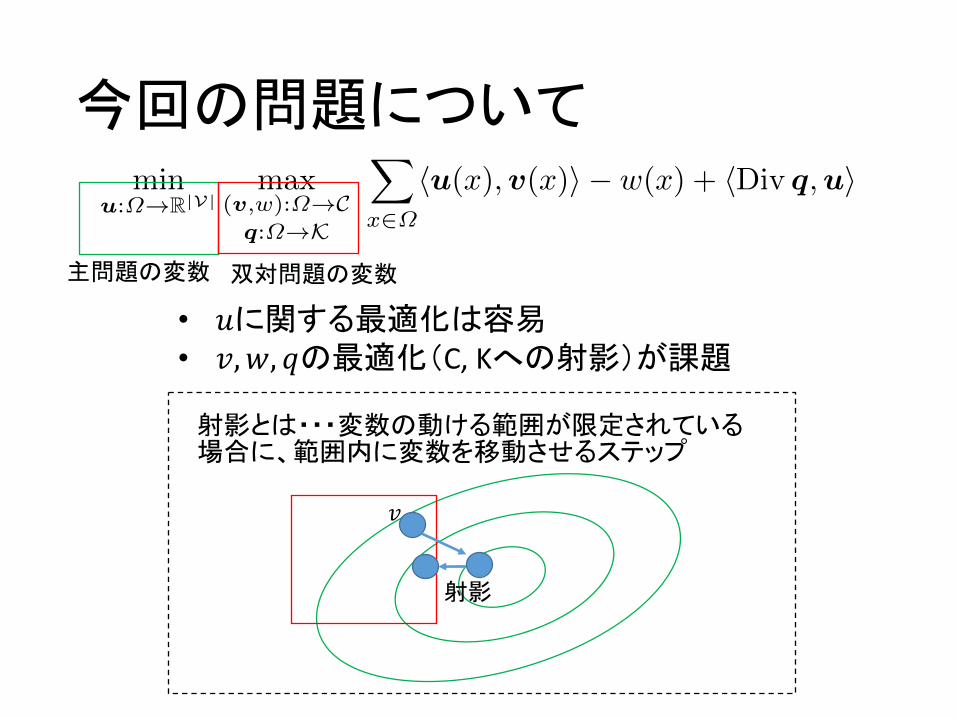
今回の問題について
Sublabel-Accurate Convex Relaxation of Vectorial Multilabel Energies 9
3 Numerical Optimization
3.1 Discretization
For now assume that ⌦ ⇢ Rd is a d-dimensional Cartesian grid and let Div
denote a finite-di↵erence divergence operator with Div q : ⌦ ! R|V|. Then the
relaxed energy minimization problem becomes
minu:⌦!R|V|
maxq:⌦!K
X
x2⌦
⇢⇤⇤(x,u(x)) + hDiv q,ui. (18)
In order to get rid of the pointwise maximum over ⇢⇤i
(v) in Eq. (8), we introduce
additional variables w(x) 2 R and additional constraints (v(x), w(x)) 2 C, x 2 ⌦
so that w(x) attains the value of the pointwise maximum:
minu:⌦!R|V|
max(v,w):⌦!Cq:⌦!K
X
x2⌦
hu(x),v(x)i � w(x) + hDiv q,ui, (19)
where the set C is given as
C =\
1i|T |
Ci
, Ci
:=n
(x, y) 2 R|V|+1 | ⇢⇤i
(x) y
o
. (20)
For numerical optimization we use a GPU-based implementation1 of a first-order
primal-dual method [14]. The algorithm requires the orthogonal projections of
the dual variables onto the sets C respectively K in every iteration. However, the
projection onto an epigraph of dimension |V| + 1 is di�cult for large values of
|V|. We rewrite the constraints (v(x), w(x)) 2 Ci
, 1 i |T |, x 2 ⌦ as (n+ 1)-
dimensional epigraph constraints introducing variables ri(x) 2 Rn, si
(x) 2 R:
⇢
⇤i
�
r
i(x)�
s
i
(x), r
i(x) = A
>i
E
>i
v(x), s
i
(x) = w(x)� hEi
b
i
,v(x)i. (21)
These equality constraints can be implemented using Lagrange multipliers. For
the projection onto the set K we use an approach similar to [7, Figure 7].
3.2 Epigraphical Projections
Computing the Euclidean projection onto the epigraph of ⇢⇤i
is a central part
of the numerical implementation of the presented method. However, for n > 1
this is nontrivial. Therefore we provide a detailed explanation of the projection
methods used for di↵erent classes of ⇢i
. We will consider quadratic, truncated
quadratic and piecewise linear ⇢.
1https://github.com/tum-vision/sublabel_relax
主問題の変数 双対問題の変数
• 𝑢に関する最適化は容易• 𝑣,𝑤, 𝑞の最適化(C,Kへの射影)が課題
𝑣
射影
射影とは・・・変数の動ける範囲が限定されている場合に、範囲内に変数を移動させるステップ
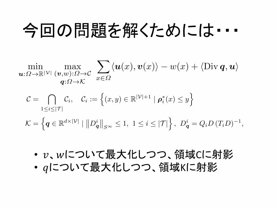
今回の問題を解くためには・・・
Sublabel-Accurate Convex Relaxation of Vectorial Multilabel Energies 9
3 Numerical Optimization
3.1 Discretization
For now assume that ⌦ ⇢ Rd is a d-dimensional Cartesian grid and let Div
denote a finite-di↵erence divergence operator with Div q : ⌦ ! R|V|. Then the
relaxed energy minimization problem becomes
minu:⌦!R|V|
maxq:⌦!K
X
x2⌦
⇢⇤⇤(x,u(x)) + hDiv q,ui. (18)
In order to get rid of the pointwise maximum over ⇢⇤i
(v) in Eq. (8), we introduce
additional variables w(x) 2 R and additional constraints (v(x), w(x)) 2 C, x 2 ⌦
so that w(x) attains the value of the pointwise maximum:
minu:⌦!R|V|
max(v,w):⌦!Cq:⌦!K
X
x2⌦
hu(x),v(x)i � w(x) + hDiv q,ui, (19)
where the set C is given as
C =\
1i|T |
Ci
, Ci
:=n
(x, y) 2 R|V|+1 | ⇢⇤i
(x) y
o
. (20)
For numerical optimization we use a GPU-based implementation1 of a first-order
primal-dual method [14]. The algorithm requires the orthogonal projections of
the dual variables onto the sets C respectively K in every iteration. However, the
projection onto an epigraph of dimension |V| + 1 is di�cult for large values of
|V|. We rewrite the constraints (v(x), w(x)) 2 Ci
, 1 i |T |, x 2 ⌦ as (n+ 1)-
dimensional epigraph constraints introducing variables ri(x) 2 Rn, si
(x) 2 R:
⇢
⇤i
�
r
i(x)�
s
i
(x), r
i(x) = A
>i
E
>i
v(x), s
i
(x) = w(x)� hEi
b
i
,v(x)i. (21)
These equality constraints can be implemented using Lagrange multipliers. For
the projection onto the set K we use an approach similar to [7, Figure 7].
3.2 Epigraphical Projections
Computing the Euclidean projection onto the epigraph of ⇢⇤i
is a central part
of the numerical implementation of the presented method. However, for n > 1
this is nontrivial. Therefore we provide a detailed explanation of the projection
methods used for di↵erent classes of ⇢i
. We will consider quadratic, truncated
quadratic and piecewise linear ⇢.
1https://github.com/tum-vision/sublabel_relax
8 E. Laude, T. Mollenho↵, M. Moeller, J. Lellmann, D. Cremers
Proof. Follows from a calculation starting at the definition of the convex conju-
gate ⇤. See Appendix A.
Interestingly, although in its original formulation (14) the set K has infinitely
many constraints, one can equivalently represent K by finitely many.
Proposition 3 The set K in equation (14) is the same as
K =n
q 2 Rd⇥|V| |�
�
D
i
q
�
�
S
1 1, 1 i |T |o
, D
i
q = Q
i
D (Ti
D)�1, (15)
where the matrices Q
i
D 2 Rd⇥n
and T
i
D 2 Rn⇥n
are given as
Q
i
D :=�
qi1 � qin+1, . . . , qin � qin+1
�
, T
i
D :=�
t
i1 � t
in+1, . . . , t
in � t
in+1�
.
Proof. Similar to the analysis in [11], equation (14) basically states the Lipschitz
continuity of a piecewise linear function defined by the matrices q 2 Rd⇥|V|.
Therefore, one can expect that the Lipschitz constraint is equivalent to a bound
on the derivative. For the complete proof, see Appendix A.
2.4 Lifting the Overall Optimization Problem
Combining dataterm and regularizer, the overall optimization problem is given
minu:⌦!R|V|
supq:⌦!K
Z
⌦
⇢⇤⇤(u) + hu,Div qi dx. (16)
A highly desirable property is that, opposed to any other vectorial lifting ap-
proach from the literature, our method with just one simplex applied to a convex
problem yields the same solution as the unlifted problem.
Proposition 4 If the triangulation contains only 1 simplex, T = {�}, i.e.,
|V| = n+ 1, then the proposed optimization problem (16) is equivalent to
minu:⌦!�
Z
⌦
(⇢+ �
�
)⇤⇤(x, u(x)) dx+ �TV (u), (17)
which is (1) with a globally convexified dataterm on �.
Proof. For u = t
n+1+TDu the substitution u =⇣
u1, . . . , un
, 1�P
n
j=1 uj
⌘
into
⇢⇤⇤ and R yields the result. For a complete proof, see Appendix A.
• 𝑣、𝑤について最大化しつつ、領域Cに射影• 𝑞について最大化しつつ、領域Kに射影
射影について
Sublabel-Accurate Convex Relaxation of Vectorial Multilabel Energies 9
3 Numerical Optimization
3.1 Discretization
For now assume that ⌦ ⇢ Rd is a d-dimensional Cartesian grid and let Div
denote a finite-di↵erence divergence operator with Div q : ⌦ ! R|V|. Then the
relaxed energy minimization problem becomes
minu:⌦!R|V|
maxq:⌦!K
X
x2⌦
⇢⇤⇤(x,u(x)) + hDiv q,ui. (18)
In order to get rid of the pointwise maximum over ⇢⇤i
(v) in Eq. (8), we introduce
additional variables w(x) 2 R and additional constraints (v(x), w(x)) 2 C, x 2 ⌦
so that w(x) attains the value of the pointwise maximum:
minu:⌦!R|V|
max(v,w):⌦!Cq:⌦!K
X
x2⌦
hu(x),v(x)i � w(x) + hDiv q,ui, (19)
where the set C is given as
C =\
1i|T |
Ci
, Ci
:=n
(x, y) 2 R|V|+1 | ⇢⇤i
(x) y
o
. (20)
For numerical optimization we use a GPU-based implementation1 of a first-order
primal-dual method [14]. The algorithm requires the orthogonal projections of
the dual variables onto the sets C respectively K in every iteration. However, the
projection onto an epigraph of dimension |V| + 1 is di�cult for large values of
|V|. We rewrite the constraints (v(x), w(x)) 2 Ci
, 1 i |T |, x 2 ⌦ as (n+ 1)-
dimensional epigraph constraints introducing variables ri(x) 2 Rn, si
(x) 2 R:
⇢
⇤i
�
r
i(x)�
s
i
(x), r
i(x) = A
>i
E
>i
v(x), s
i
(x) = w(x)� hEi
b
i
,v(x)i. (21)
These equality constraints can be implemented using Lagrange multipliers. For
the projection onto the set K we use an approach similar to [7, Figure 7].
3.2 Epigraphical Projections
Computing the Euclidean projection onto the epigraph of ⇢⇤i
is a central part
of the numerical implementation of the presented method. However, for n > 1
this is nontrivial. Therefore we provide a detailed explanation of the projection
methods used for di↵erent classes of ⇢i
. We will consider quadratic, truncated
quadratic and piecewise linear ⇢.
1https://github.com/tum-vision/sublabel_relax
8 E. Laude, T. Mollenho↵, M. Moeller, J. Lellmann, D. Cremers
Proof. Follows from a calculation starting at the definition of the convex conju-
gate ⇤. See Appendix A.
Interestingly, although in its original formulation (14) the set K has infinitely
many constraints, one can equivalently represent K by finitely many.
Proposition 3 The set K in equation (14) is the same as
K =n
q 2 Rd⇥|V| |�
�
D
i
q
�
�
S
1 1, 1 i |T |o
, D
i
q = Q
i
D (Ti
D)�1, (15)
where the matrices Q
i
D 2 Rd⇥n
and T
i
D 2 Rn⇥n
are given as
Q
i
D :=�
qi1 � qin+1, . . . , qin � qin+1
�
, T
i
D :=�
t
i1 � t
in+1, . . . , t
in � t
in+1�
.
Proof. Similar to the analysis in [11], equation (14) basically states the Lipschitz
continuity of a piecewise linear function defined by the matrices q 2 Rd⇥|V|.
Therefore, one can expect that the Lipschitz constraint is equivalent to a bound
on the derivative. For the complete proof, see Appendix A.
2.4 Lifting the Overall Optimization Problem
Combining dataterm and regularizer, the overall optimization problem is given
minu:⌦!R|V|
supq:⌦!K
Z
⌦
⇢⇤⇤(u) + hu,Div qi dx. (16)
A highly desirable property is that, opposed to any other vectorial lifting ap-
proach from the literature, our method with just one simplex applied to a convex
problem yields the same solution as the unlifted problem.
Proposition 4 If the triangulation contains only 1 simplex, T = {�}, i.e.,
|V| = n+ 1, then the proposed optimization problem (16) is equivalent to
minu:⌦!�
Z
⌦
(⇢+ �
�
)⇤⇤(x, u(x)) dx+ �TV (u), (17)
which is (1) with a globally convexified dataterm on �.
Proof. For u = t
n+1+TDu the substitution u =⇣
u1, . . . , un
, 1�P
n
j=1 uj
⌘
into
⇢⇤⇤ and R yields the result. For a complete proof, see Appendix A.
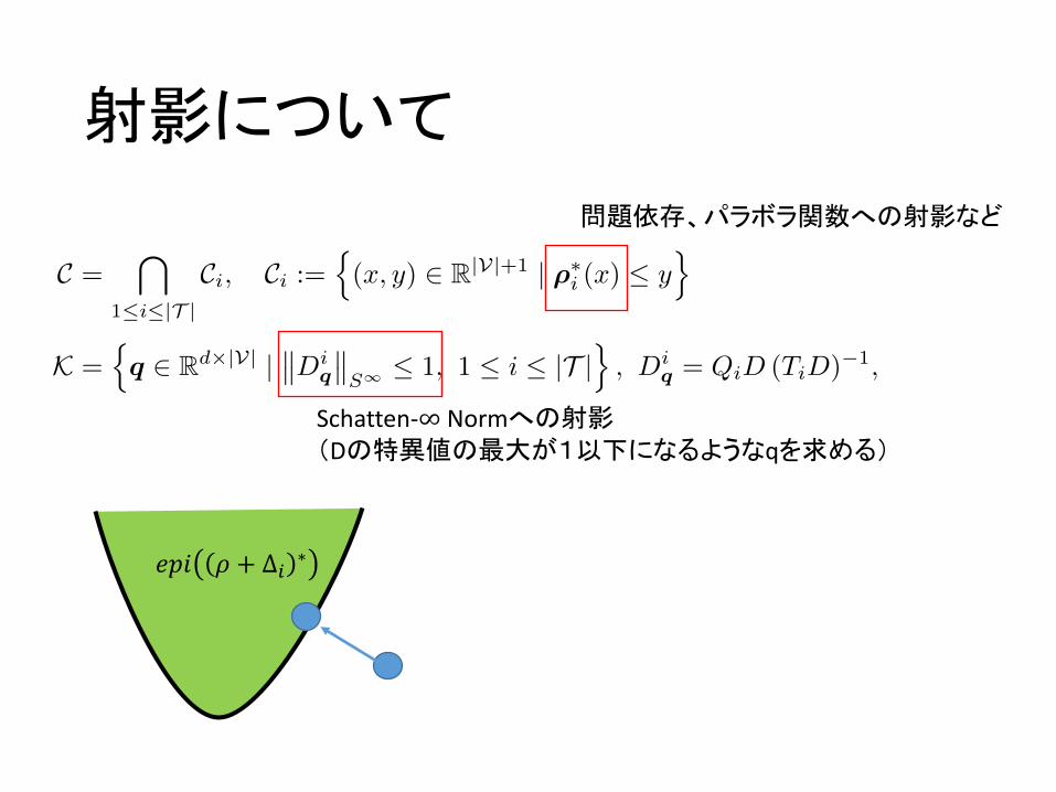
Schatten-∞ Normへの射影(Dの特異値の最大が1以下になるようなqを求める)
問題依存、パラボラ関数への射影など
𝑒𝑝𝑖 𝜌 + ∆R ∗
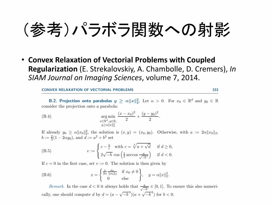
(参考)パラボラ関数への射影
• ConvexRelaxationofVectorialProblemswithCoupledRegularization (E.Strekalovskiy,A.Chambolle,D.Cremers), InSIAMJournalonImagingSciences,volume7,2014.
CONVEX RELAXATION OF VECTORIAL PROBLEMS 333
B.2. Projection onto parabolas y ≥ α∥x∥22. Let α > 0. For x0 ∈ Rd and y0 ∈ Rconsider the projection onto a parabola:
(B.4) argminx∈Rd, y∈R,y≥α∥x∥22
(x− x0)2
2+
(y − y0)2
2.
If already y0 ≥ α∥x0∥22, the solution is (x, y) = (x0, y0). Otherwise, with a := 2α∥x0∥2,b := 2
3(1− 2αy0), and d := a2 + b3 set
(B.5) v :=
⎧⎨
⎩c− b
c with c =3√
a+√d if d ≥ 0,
2√−b cos
(13 arccos
a√−b
3
)if d < 0.
If c = 0 in the first case, set v := 0. The solution is then given by
(B.6) x =
{v2α
x0∥x0∥2 if x0 = 0
0 else
}, y = α∥x∥22.
Remark. In the case d < 0 it always holds that a√−b
3 ∈ [0, 1]. To ensure this also numeri-
cally, one should compute d by d = (a−√−b
3)(a+
√−b
3) for b < 0.
Proof. First, for y0 ≥ α∥x0∥22 the projection is obviously (x, y) = (x0, y0). Otherwise, wedualize the parabola constraint using δz≥0 = supλ≥0−λz (for z ∈ R):
(B.7) minx∈Rd, y∈R
maxλ≥0
(x− x0)2
2+
(y − y0)2
2− λ
(y − α∥x∥22
).
Since this expression is convex in x, y and concave in λ, we can interchange the ordering ofmin and max. The inner minimization problem in x and y is then easily solved, giving thefollowing necessary representation, with a certain λ ≥ 0:
(B.8) x =x0
1 + 2αλ, y = y0 + λ.
For instance, x has the same direction as x0, so only the norm of x is unknown. The solutionmust also necessarily satisfy y = α∥x∥22. Plugging this into the second equation of (B.8), aswell as the expression for λ obtained from the first equation by taking the norms, we obtainthe cubic equation
(B.9) 2α2∥x∥32 + (1− 2αy0)∥x∥2 − ∥x0∥2 = 0.
Set a := 2α∥x0∥2, b := 23 (1− 2αy0), and t := 2α∥x∥2. Then (B.9) becomes
(B.10) t3 + 3bt− 2a = 0.
Since the derivative 3t2 + 3b of the left-hand side is monotonically increasing for t ≥ 0, thet we are looking for is the unique nonnegative solution of (B.10) for x0 = 0 (so that a > 0).This cubic equation can be solved using the method of elementary hyperbolic/trigonometricfunction identities [30], yielding the claimed solution. The second case in (B.5) correspondsto “x2” in equation (23) of [30].
For x0 = 0, because of the assumed inequality y0 < α∥x0∥22 = 0 we have the first case in(B.5), which leads to the correct solution (x, y) = (0, 0).
(参考) Schatten-∞ Normへの射影
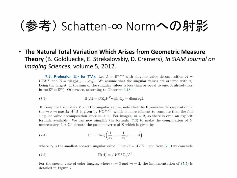
• TheNaturalTotalVariationWhichArisesfromGeometricMeasureTheory (B.Goldluecke,E.Strekalovskiy,D.Cremers), InSIAMJournalonImagingSciences,volume5,2012.
Copyright © by SIAM. Unauthorized reproduction of this article is prohibited.
VECTORIAL TOTAL VARIATION 555
in that color edges are preserved better. We also showed that TVJ can serve as a regularizerin more general energy functionals, which makes it applicable to general inverse problems likedeblurring, zooming, inpainting, and superresolution.
7.1. Projection ΠS for TVS. Since each channel is treated separately, we can computethe well-known projection for the scalar TV for each color channel. Let A ∈ Rn×m with rowsa1, . . . , an ∈ Rm. Then ΠS is defined rowwise as
(7.1) ΠS(ai) =ai
max(1, |ai|2).
7.2. Projection ΠF for TVF . Let A ∈ Rn×m with elements aij ∈ R. From (2.8) we seethat we need to compute the projection onto the unit ball in Rn·m when (aij) is viewed as avector in Rn·m. Thus,
(7.2) ΠF (A) =A
max!1,"#n
i=1
#mj=1 a
2ij
$ .
7.3. Projection ΠJ for TVJ . Let A ∈ Rn×m with singular value decomposition A =UΣV T and Σ = diag(σ1, . . . ,σm). We assume that the singular values are ordered with σ1being the largest. If the sum of the singular values is less than or equal to one, A already liesin co(En ⊗ Em). Otherwise, according to Theorem 3.18,
(7.3) Π(A) = UΣpVTwith Σp = diag(σp).
To compute the matrix V and the singular values, note that the Eigenvalue decomposition ofthe m×m matrix ATA is given by V Σ2V T , which is more efficient to compute than the fullsingular value decomposition since m < n. For images, m = 2, so there is even an explicitformula available. We can now simplify the formula (7.3) to make the computation of Uunnecessary. Let Σ+ denote the pseudoinverse of Σ which is given by
(7.4) Σ+ = diag
%1
σ1, . . . ,
1
σk, 0, . . . , 0
&,
where σk is the smallest nonzero singular value. Then U = AV Σ+, and from (7.3) we conclude
(7.5) Π(A) = AV Σ+ΣpVT .
For the special case of color images, where n = 3 and m = 2, the implementation of (7.5) isdetailed in Figure 7.
Appendix A. In this appendix we show explicitly how to compute the projection ΠK :Rn×m → Rn×m required for the algorithms in Figure 8 for the different types of vectorial totalvariation. In all cases, ΠK is the orthogonal projection onto a closed convex set K, which isgiven for the different regularizers in (5.3).
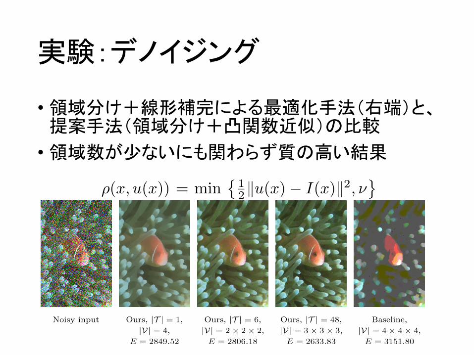
実験:デノイジング
• 領域分け+線形補完による最適化手法(右端)と、提案手法(領域分け+凸関数近似)の比較
• 領域数が少ないにも関わらず質の高い結果
12 E. Laude, T. Mollenho↵, M. Moeller, J. Lellmann, D. Cremers
Input image Unlifted Problem,
E = 992.50
Ours, |T | = 1,
|V| = 4,
E = 992.51
Ours, |T | = 6
|V| = 2 ⇥ 2 ⇥ 2
E = 993.52
Baseline,
|V| = 4 ⇥ 4 ⇥ 4,
E = 2255.81
Fig. 5: Convex ROF with vectorial TV. Direct optimization and proposed method
yield the same result. In contrast to the baseline method [11] the proposed ap-
proach has no discretization artefacts and yields a lower energy. The regulariza-
tion parameter is chosen as � = 0.3.
Noisy input Ours, |T | = 1,
|V| = 4,
E = 2849.52
Ours, |T | = 6,
|V| = 2 ⇥ 2 ⇥ 2,
E = 2806.18
Ours, |T | = 48,
|V| = 3 ⇥ 3 ⇥ 3,
E = 2633.83
Baseline,
|V| = 4 ⇥ 4 ⇥ 4,
E = 3151.80
Fig. 6: ROF with a truncated quadratic dataterm (� = 0.03 and ⌫ = 0.025).
Compared to the baseline method [11] the proposed approach yields much better
results, already with a very small number of 4 labels.
using the epigraph decomposition described in the second paragraph of Sec. 3.2.
It can be seen, that increasing the number of labels |V| leads to lower energies andat the same time to a reduced e↵ect of the TV. This occurs as we always compute
a piecewise convex underapproximation of the original nonconvex dataterm, that
gets tighter with a growing number of labels. The baseline method [11] again
produces strong discretization artefacts even for a large number of labels |V| =4⇥ 4⇥ 4 = 64.
Sublabel-Accurate Convex Relaxation of Vectorial Multilabel Energies 11
-1 0 1-1
0
1
Naive, 81 labels.
-1 0 1-1
0
1
[11], 81 labels.
�1 1�1
1
Ours, 4 labels.
Fig. 4: ROF denoising of a vector-valued signal f : [0, 1] ! [�1, 1]2, discretized
on 50 points (shown in red). We compare the proposed approach (right) with
two alternative techniques introduced in [11] (left and middle). The labels are
visualized by the gray grid. While the naive (standard) multilabel approach from
[11] (left) provides solutions that are constrained to the chosen set of labels, the
sublabel accurate regularizer from [11] (middle) does allow sublabel solutions,
yet – due to the dataterm bias – these still exhibit a strong preference for the grid
points. In contrast, the proposed approach does not exhibit any visible grid bias
providing fully sublabel-accurate solutions: With only 4 labels, the computed
solutions (shown in blue) coincide with the “unlifted” problem (green).
4 Experiments
4.1 Vectorial ROF Denoising
In order to validate experimentally, that our model is exact for convex dataterms,
we evaluate it on the Rudin-Osher-Fatemi [18] (ROF) model with vectorial
TV (2). In our model this corresponds to defining ⇢(x, u(x)) = 12ku(x)� I(x)k2.
As expected based on Prop. 4 the energy of the solution of the unlifted problem
is equal to the energy of the projected solution of our method for |V| = 4 up to
machine precision, as can be seen in Fig. 4 and Fig. 5. We point out, that the
sole purpose of this experiment is a proof of concept as our method introduces
an overhead and convex problems can be solved via direct optimization. It can
be seen in Fig. 4 and Fig. 5, that the baseline method [11] has a strong label
bias.
4.2 Denoising with Truncated Quadratic Dataterm
For images degraded with both, Gaussian and salt-and-pepper noise we define
the dataterm as ⇢(x, u(x)) = min�
12ku(x)� I(x)k2, ⌫
. We solve the problem

実験:オプティカルフローΩ
Sublabel-Accurate Convex Relaxation of Vectorial Multilabel Energies 13
Image 1 [8], |V| = 5 ⇥ 5,
0.67 GB, 4 min
aep = 2.78
[8], |V| = 11 ⇥ 11,
2.1 GB, 12 min
aep = 1.97
[8], |V| = 17 ⇥ 17,
4.1 GB, 25 min
aep = 1.63
[8], |V| = 28 ⇥ 28,
9.3 GB, 60 min
aep = 1.39
Image 2 [11], |V| = 3 ⇥ 3,
0.67 GB, 0.35 min
aep = 5.44
[11], |V| = 5 ⇥ 5,
2.4 GB, 16 min
aep = 4.22
[11], |V| = 7 ⇥ 7,
5.2 GB, 33 min
aep = 2.65
[11], |V| = 9 ⇥ 9,
Out of memory.
Ground truth Ours, |V| = 2 ⇥ 2,
0.63 GB, 17 min
aep = 1.28
Ours, |V| = 3 ⇥ 3,
1.9 GB, 34 min
aep = 1.07
Ours, |V| = 4 ⇥ 4,
4.1 GB, 41 min
aep = 0.97
Ours, |V| = 6 ⇥ 6,
10.1 GB, 56 min
aep = 0.9
Fig. 7: We compute the optical flow using our method, the product space ap-
proach [8] and the baseline method [11] for a varying amount of labels and
compare the average endpoint error (aep). The product space method clearly
outperforms the baseline, but our approach finds the overall best result already
with 2 ⇥ 2 labels. To achieve a similarly precise result as the product space
method, we require 150 times fewer labels, 10 times less memory and 3 times
less time. For the same number of labels, the proposed approach requires more
memory as it has to store a convex approximation of the energy instead of a
linear one.
4.3 Optical Flow
We compute the optical flow v : ⌦ ! R2 between two input images I1, I2.
The label space � = [�d, d]2 is chosen according to the estimated maximum
displacement d 2 R between the images. The dataterm is ⇢(x, v(x)) = kI2(x)�I1(x+ v(x))k, and �(x) is based on the norm of the image gradient rI1(x).
In Fig. 7 we compare the proposed method to the product space approach
[8]. Note that we implemented the product space dataterm using Lagrange mul-
• 領域分け+線形補完による最適化手法(右端)と、提案手法(領域分け+凸関数近似)の比較
• 領域数が少ないにも関わらず質の高い結果
まとめ
• 多次元のマルチラベル問題の一般解法を提案
• 凸関数で近似することで高精度な解を出力
• VectorialTotalVariationによる質の高い正則化
Recommended


![Sublabel-Accurate Convex Relaxation of Vectorial ... · Sublabel-Accurate Convex Relaxation of Vectorial Multilabel Energies 3 In a series of papers [5,6], connections of the above](https://img.pdfslide.net/doc/110x75/5ec59c20150d306a517bf7f3/sublabel-accurate-convex-relaxation-of-vectorial-sublabel-accurate-convex-relaxation.jpg)