Supply Chain Control:
A Theory of Vertical Integration∗†
Giovanni Ursino
Universitat Pompeu Fabra
and
Universita Ca’Foscari
October 8, 2008
Abstract
Improving a company’s bargaining position is often cited as a chief mo-
tivation to vertically integrate with suppliers. This paper expands on that
view in building a new theory of vertical integration. In my model firms
integrate to gain bargaining power against other suppliers in the produc-
tion process. The cost of integration is a loss of flexibility in choosing the
most suitable suppliers for a particular final product. I show that the firms
who make the most specific investments in the production process have the
greatest incentive to integrate. The theory provides novel insights to the
understanding of numerous stylized facts such as the effect of financial de-
velopment on the vertical structure of firms, the observed pattern from FDI
to outsourcing in international trade, the effect of technological obsolescence
on organizations, etc.
Keywords: vertical integration, supply chain, bargaining, outside options
∗I am grateful to Markus Mobius for his advice, to Filippo Balestrieri, Milo Bianchi andPaul Niehaus for discussions, and to seminar participants at Harvard and UPF. I gratefullyacknowledge financial support from the Associazione Borsisti Marco Fanno.
†This paper was written when the author was visiting the Department of Economics atHarvard University.
1 Introduction
I consider how vertical integration affects the bargaining power of the integrat-
ing firms against non-integrated firms in the supply chain. Integration has costs
because it limits an assembler’s flexibility in choosing the most suitable suppliers
for a particular end product. However, by gaining bargaining power the assembler
can appropriate a larger share of the total revenue which can make integration a
profitable strategy for the assembler.
I use two examples from the PC and the cell phone industry to motivate my
analysis. In the PC industry, IBM and Apple Inc. followed very different strategies.
IBM only controlled the hardware of the original PC and had Microsoft provide the
operating system. In contrast, Apple controlled both the operating system and the
hardware of the Macintosh PC from the start. Within a few short years, Microsoft
became the dominant player in the PC industry and in 2005 IBM exited the PC
business by selling its remaining factories. Apple, on the other hand, was able
to keep its PC business highly profitable and thriving. Apple’s decision did not
come without costs because the company was often slow in updating its operating
system.1 Ultimately, however, Apple’s decision to integrate software and hardware
and sacrifice flexibility proved profitable. In the cell phone industry, there has
been substantial disagreement about the optimal level of vertical integration and
the boundary between in-house and outside procurement has shifted a number of
time during the past 15 years. In the 1990s, large handset manufacturers such
as Motorola, Nokia and Ericsson outsourced a lot of the design and software de-
velopment to suppliers in Taiwan, Singapore and India. These suppliers gained
crucial knowledge and expertise as a result which allowed some of them to be-
come fierce competitors on their own right.2 The business press has acknowledged
the importance of vertical integration for bargaining with suppliers. For example,
the Financial Times stated in a special report on vertical integration that “An-
1For example, Windows 95 was considered a more stable system than the Apple OS 7. Infact, the main reason behind IBM’s decision not to develop the operating system in-house was adesire to bring the PC to market as quickly as possible.
2For example, HTC now produces own brand smart phones as well as those of its clients.The same is true for Compal and the goal of Flextronics’ CEO Michael E. Marks -as reportedby Business Week (March 21, 2005)- is to make Flextronics a low-cost, soup-to-nuts developer ofconsumer-electronics and tech gear.
1

other reason to integrate vertically is to affect bargaining power with suppliers”
(November 29, 1999).
In my model, each final product requires a continuum of inputs which are each
produced by a specialized supplier. Inputs in my model are complements and
each supplier has ex-ante equal ability to hold up assembly of the final product.
I assume that inputs differ in their specificity, defined by the extent to which
the revenue produced by each supplier is subject to hold up. The assembler of
the final product has the opportunity to purchase suppliers and integrate them
into a single company. The integrated company obtains bargaining power that is
disproportionately larger than the share of the production process that is being
integrated in the single company. In return, the assembler loses the ability to
choose the most suitable companies for production of the final product.
As long as the inefficiency that is caused by integration is not too severe a well
defined integrated equilibrium exists. I show that the vertically integrated com-
pany will incorporate those suppliers who are required to make the most specific
investments. The intuition behind this result is that those suppliers are most vul-
nerable to hold-up and therefore benefit the most from an increase in bargaining
power. In my basic model, integration always has negative welfare consequences
because integration affects the distribution of revenue between integrated and non-
integrated firms but actually decreases total available revenue (due to the decrease
in flexibility). In an extension of the model I allow firms to vary the level of
investment. I show that, in certain conditions, integration can improve welfare be-
cause firms with specific investments will invest more after integration since their
investments are better shielded from expropriation.
My model predicts that a greater incidence of incremental innovation, the in-
creased human to physical capital ratio and the rise of modern financial markets
(Rajan and Zingales (2001); Acemoglu, Johnson, and Mitton (2005)) lead to less
vertical integration which is consistent with recent trends in developed economies.
On the other hand, I also show that industries with a high level of basic research
give rise to vertically integrated firms (see Acemoglu, Aghion, Griffith, and Zili-
botti (2004)). The prediction that the vertically integrated company incorporates
those suppliers who are required to make the most specific investments explains
why Japanese auto makers have historically been unwilling to import US auto parts
2
with high technological content (Spencer and Qiu (2001); Qiu and Spencer (2002)).
My model also helps to explain why vertically integrated firms are mostly found
in developed countries while developing countries host predominantly small-sized
firms. Using a similar approach as in Antras (2005) my model can also explain
the recent shift from FDI to outsourcing in international trade (see also Vernon
(1966)).
My work shares several characteristics with the Property Rights theory of the
firm as developed in Grossman and Hart (1986) and Hart and Moore (1990). Just
as in the property-rights view firms’ investments can be appropriated by a partner.
However, my model analyzes the bargaining power of integrated (inside) firms ver-
sus non-integrated (outside) firms. My model also contributes to our understanding
of the optimal boundary of the firm. This question was famously posed by Coase
(1937) and became the cornerstone of Transaction Cost Economics (Williamson
(1985), Williamson (2002)). Although my model resembles models found in the
literature on vertical foreclosure (Salinger (1988), Hart and Tirole (1990), Kranton
and Minehart (2002)) the mechanism is quite different. In the foreclosure liter-
ature different assemblers produce an homogeneous final good and compete with
each other - integration serves as a means to exclude the competing assembler from
access to crucial supplier. In contrast, each assembler in my model is a monopolist
in the final product market. Finally, my model shares some features of Acemoglu,
Antras, and Helpman (2007), most notably the way contractual incompleteness is
modeled -more on this later.
In the next section I introduce and analyze the basic model. Section 3 endog-
enizes the investment decision of firms. In section 4 I apply the model to explain
a series of stylized facts. Section 5 concludes.
2 Theory
This section introduces a simple model that exhibits the tradeoff between the
bargaining advantage that vertical integration provides and the loss in flexibility.
3
2.1 Model Setup
I model an industry that produces L variants of a final product (such as the
automobile industry or the cell phone industry). Each final product variant is
assembled from a set of individual essential components3 which I index by i ∈ [0, 1].
Each type i component is produced by a type i firm. Since there are different
variants there are also multiple firms of each type, one per variant. Components
are put together by an assembler - there is one assembler for each final product
variant.
Each component can be either “perfect” or imperfect for the final product.
The share of perfect components in a product, x, determines the value of the final
product variant in the market. For the sake of simplicity I assume a simple linear
specification and define the final revenue, S, as:
S = πx (1)
In order to produce each firm has to make an investment of 1. Therefore, total
profits for a final product variant with a share x of perfect components are πx− 1.
Firms differ in their ability to appropriate the available revenue S. I as-
sume that each firm type i can appropriate a revenue of r(i)S by investing where
r(i) is an increasing function that lies between 0 and 1. The remaining revenue
S =∫ 1
0[1 − r(i)] S is subject to negotiation between firms which I describe in
greater detail below. The function r(i) is the specificity function and captures the
extent to which a firm’s claim to the revenue is subject to negotiation between
firms. For example, the revenue of a firm with specificity r(i) = 0 fully depends
on its ability to negotiate with other component suppliers. On the other hand, a
firm with specificity r(i) = 1 does not have to rely on negotiation at all. I con-
sider the specificity function as determined by production technology4. In section
3A final product cannot be produced and/or sold without each and every component, hencecomponents are essential. In other words, the production function is Leontief.
4Modeling investment specificity without reference to the existence of a second best market isnot novel. For instance Acemoglu, Antras, and Helpman (2007) model contractual incompletenessby allowing suppliers’ activities to be only partially verifiable: the degree of verifiability of asupplier’s activities is a primitive in their model and determines her bargaining outcome.
Moreover a large literature [...] attests that, when writing provisions for the breach of acontract, businessmen don’t actually believe they have a way out the contract failure other than
4
4 I analyze how vertical integration decisions differ across industries with different
specificity functions.
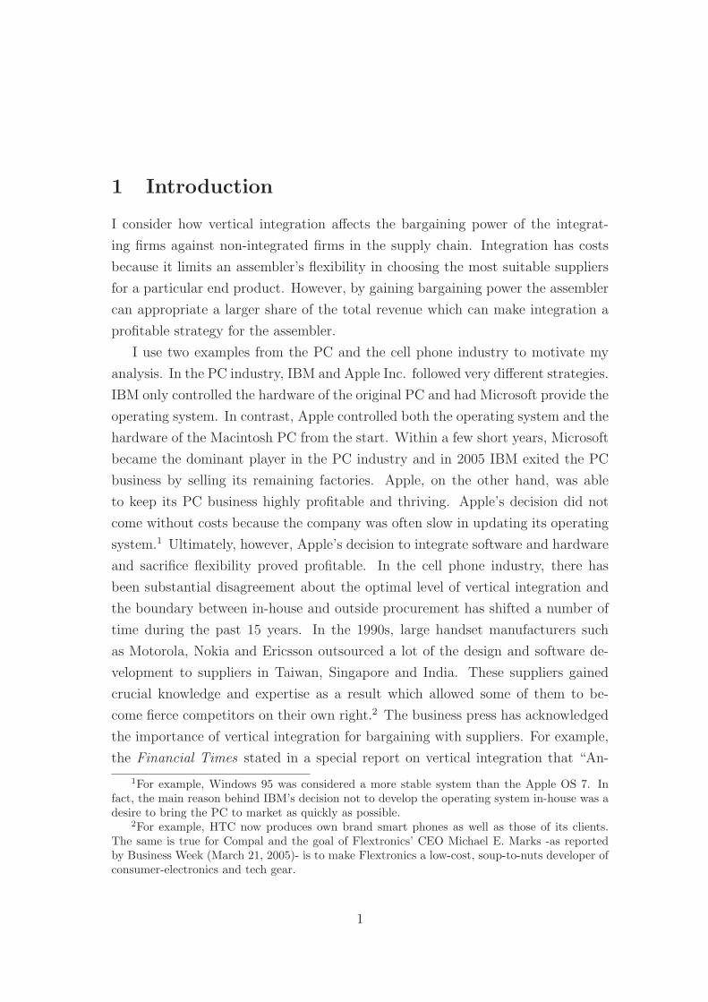
Figure 1: Timing for vertical integration game and negotiation over revenue
Assemblers buysubset
of suppliers
Stage 1
-
Firms alignwith
assemblers
Stage 2
-Firms makeinvestments
Stage 3
-Revenueis divided
Stage 4
The remainder of the model describes precisely how firms divide the appro-
priable revenue S among themselves and how they can affect the distribution of
revenue through vertical integration. Figure 1 lists the four main stages of the
model.
Stage 1: Vertical Integration Game
In the first period each assembler can buy a subset I ⊂ [0, 1] of component
firms and form a vertically integrated firm. To simplify notation I will focus on the
cases where assemblers use symmetric strategies such that each assembler buys the
same portfolio of firms. I will later show that the assemblers will prefer to buy a
contiguous set of firms I = [0, N ] where 0 ≤ N ≤ 1 and N =∫
Idi. However, the
model does not restrict assemblers to such strategies
In equilibrium the assembler has to offer each firm the profit the firm would
derive from remaining non-integrated.
Stage 2: Alignment Stage
In the second period non-integrated firms choose assemblers. I assume that
each non-integrated firm of type i produces a “perfect” component for exactly one
final product variant. For all other variants the firm’s component is non-perfect.
This gives rise to a simple assignment of non-integrated firms to assemblers: each
type i firm will choose its optimal variant.
I assume that each component produced by an integrated firm is perfect with
probability γ ≤ 1. The parameter γ is determined by technology and captures the
loss of flexibility that vertical integration entails. The lower γ the more costly is
the payment of fees. In other words, when dealing with complex transactions, managers normallydon’t take it seriously the existence of an outside market for their specific components.
5
vertical integration.
Integration by itself therefore induces a welfare loss because it bounds a portfo-
lio of component suppliers together before uncertainty about a supplier’s suitability
for a particular final product variant is resolved. For example, a vertically inte-
grated car manufacturer might discover that it needs to increase the share of fuel
efficient cars in its lineup. However, because the company is integrated it might be
forced to make use of gas-guzzling internally produced engines rather than source
engines from suppliers of fuel-efficient engines5.
Stage 3: Investment Stage
In this stage all firms decide whether to invest one unit of capital. Production
of a final product variant is Leontief - therefore it cannot take place unless all
suppliers make the required investment.
Stage 4: Bargaining Stage
In the bargaining stage both integrated and non-integrated firms divide the
appropriable revenue S:
S = π(1 − N + Nγ)
∫ 1
0
[1 − r(i)] di (2)
I assume that firms engage in Nash bargaining6. One problem with Nash bargain-
ing in the presence of a vertically integrated firm is that integration tends to reduce
bargaining power. To see the problem, consider simple bargaining over a pie of
size 1 with three firms with equal bargaining power and outside option 0. Each
firm will receive 13
of the pie. Now assume that two firms integrate and bargain as
a single entity with the third firm. Now the integrated firm will receive 12
of the
pie - therefore integration hurts a firm’s bargaining power.
I follow Kalai (1977) and assume that the integrated firm has Nash weight N7.
5Of course an assembler might well procure both internally and from outside at the sametime, possibly at a higher cost. Here I focus on a more drastic in or out decision.
6Another widely used concept is the Shapley Value. I use Nash Bargaining because a) beinga non cooperative solution concept it fits better the zero-sum opportunistic nature of the gamestudied here; and b) given the Leontief production function, the marginal contribution of eachsupplier would be equal to the whole value of production and the resulting share would be triviallyequal across suppliers.
7Kalai (1977) deals with group aggregation of players in multi-players Nash bargaining prob-lems and suggests that a group be weighted by the number of its components. This implies thata group-player enjoys a share of the pie proportional to its size.
6
This implies that integration per se does neither decrease nor increase a firm’s
bargaining power. Instead, in my model the division of the pie will be affected by
the outside option of integrated and non-integrated firms.
I assume that a non-integrated firm has outside option 0. The integrated firm,
however, can replace any non-integrated firm with a fringe supplier. Fringe sup-
pliers always produce imperfect components. Therefore, if bargaining in the last
period breaks down the integrated firm will bargain with fringe suppliers in an
auxiliary bargaining round where the appropriable revenue is now8:
Saux = πNγ
∫ 1
0
[1 − r(i)] di (3)
In this auxiliary round the outside option of both integrated firm and fringe sup-
pliers is zero.
2.2 Discussion
Intuitively, in my model vertical integration improves the bargaining power of
integrating firms in the bargaining stage but prevents them from optimally mixing
and matching component suppliers to maximize the share of perfect components
when producing the final product variant.
One immediate implication of the model is that integration always decreases
welfare even though integration can be privately optimal for the assembler. This
is no longer necessarily true when investment is endogenous: if firms can vary the
amount of their investment integration can improve investment incentives for the
integrating firms because it provides a shield against expropriation at the bargain-
ing stage. Under certain conditions the welfare gain through higher investment can
offset the welfare loss from lower flexibility. I discuss this extension in section 3.
8The difference between S and Saux is that (1 − N + Nγ) is replaced by Nγ because now,given the inferior quality of fringe suppliers’ components, the only perfect components are theNγ components produced by the integrated assembler
7
2.3 Analysis
I begin the analysis with the benchmark case of uniform specificity, such that
r(i) = i. This case is analytically particularly tractable. I will later generalize the
specificity function.
2.3.1 Uniform specificity
Under uniform specificity the appropriable revenue becomes:
S = π(1 − N + Nγ)
∫ 1
0
(1 − i) di (4)
where N is the number of component firms bought by the assembler at stage 1. The
appropriable revenue is maximized when there is no integration (N = 0) because
integration always reduces productivity since integrated firms always produce a
share of non-perfect components (γ < 1).
Without integration a firm of type i which invests one unit of capital obtains πi
units of “private” revenue plus an equal9 share of the appropriable revenue through
Nash bargaining. Its profit can be written as
π
[
i +
∫ 1
0
(1 − j)dj
]
− 1 (5)
which is positive for any firm as long as π is large enough. I assume that π is large
enough to make production individually rational. It follows from (5) that firms
with the least specific investments (high i) will be more profitable than firms with
more specific investments because they are less exposed to hold-up.
I solve the model backwards by analyzing the bargaining stage where the as-
sembler has integrated N firms. Assembler and non-integrated suppliers bargain
over the appropriable revenue S. Each non integrated supplier has an outside op-
tion of zero. The outside option of the assembler, on the other hand, is whatever
can be obtained in the auxiliary bargaining round which occurs if assembler and
suppliers cannot reach agreement in the first round. In this case the appropriable
9All the firms have zero outside option in this case. The share is 1 because there is a mass 1of firms.
8
revenue is (3) and the integrated assembler is entitled to a share N of it, as pre-
scribed by Nash bargaining a la Kalai. Thus, the outside option of the integrated
assembler in the first round is πN2γ∫ 1
0(1 − i) di.
Since the integrated assembler has a better outside option than the non inte-
grated component firms, the assembler can secure a share of revenue in the first
round, F (N), which exceeds its share of production N . Formally, the assembler’s
share of appropriable revenue, F (N), solves the following Nash maximization prob-
lem:
F (N) = arg maxs
{
ln
(
sπ(1 − N + Nγ)
∫ 1
0
(1 − i) di − πN2γ
∫ 1
0
(1 − i) di
)N
+(1 − N) ln
(
1 − s
1 − Nπ(1 − N + Nγ)
∫ 1
0
(1 − i) di
)
}
(6)
The second term in this expression describes the division of revenue among the
1 − N non-integrated firms, each one receiving an equal share of the revenue not
assigned to the assembler, 1−s. The revenue share of the assembler can be derived
as:
F (N) = N +γN2(1 − N)
1 − N + γN(7)
Clearly F (N) > N and F ′(N) > 0 for any N ∈ [0, 1]: there is a bargaining
premium which comes with size. Also, F (N) = 0 for N = 0 and F (N) = 1 for
N = 1. Finally, the share of revenue of the assembler does not depend at all on
which suppliers he buys nor on the appropriable revenue generated by production,
but solely on its size and on the inefficiency parameter γ: this is because the
amount of investment is the same for all firm types.
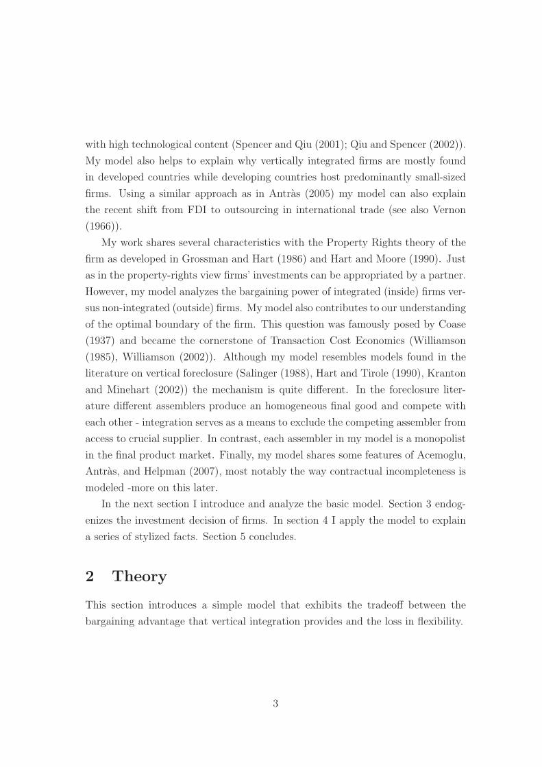
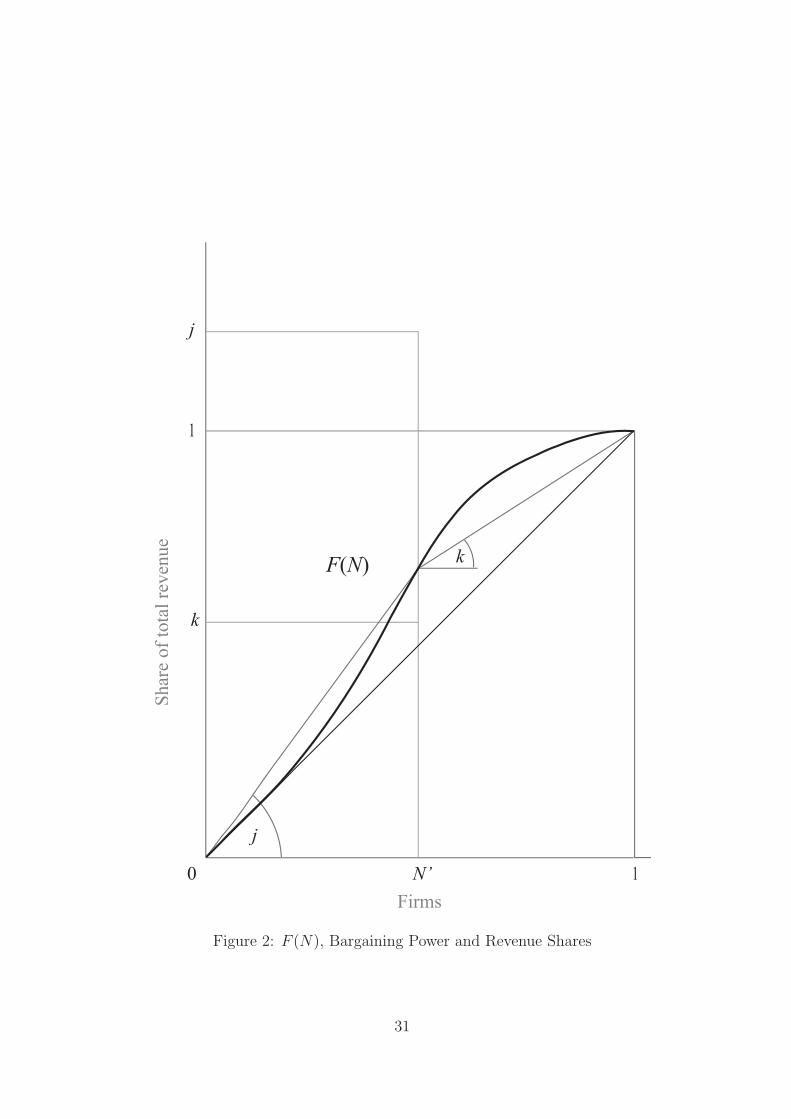
To illustrate the power balances resulting from vertical integration, notice that
the shares of revenue enjoyed by different firms can always be represented by means
of a cumulative distribution function. Figure 2 plots the cumulative share distribu-
tion as a function of N , with the corresponding shares of two representative firms:
an ideal (or average) component of the integrated firm, j, and a non integrated
firm, k. The s-shape curve indicates, for each N , the share of the corresponding
vertical integration while the 45 degrees line is the share cumulative distribution
under non integration. Under non integration each firm has a share of one. When
9
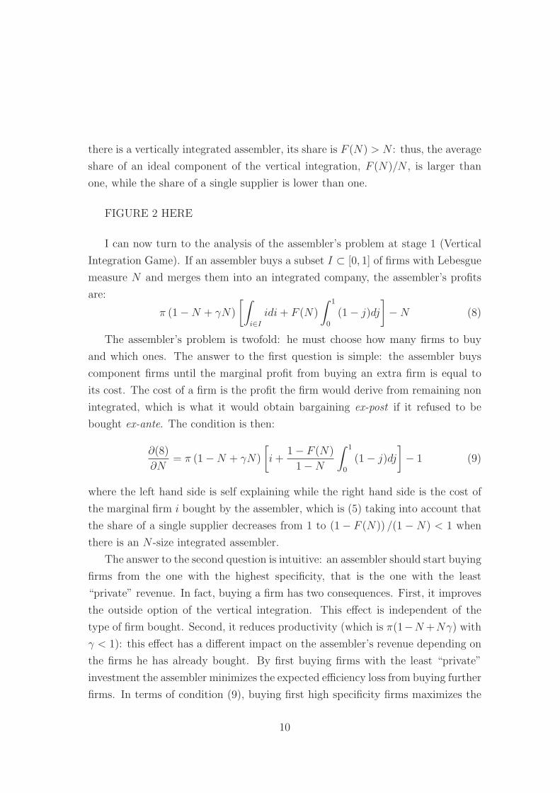
there is a vertically integrated assembler, its share is F (N) > N : thus, the average
share of an ideal component of the vertical integration, F (N)/N , is larger than
one, while the share of a single supplier is lower than one.
FIGURE 2 HERE
I can now turn to the analysis of the assembler’s problem at stage 1 (Vertical
Integration Game). If an assembler buys a subset I ⊂ [0, 1] of firms with Lebesgue
measure N and merges them into an integrated company, the assembler’s profits
are:
π (1 − N + γN)
[∫
i∈I
idi + F (N)
∫ 1
0
(1 − j)dj
]
− N (8)
The assembler’s problem is twofold: he must choose how many firms to buy
and which ones. The answer to the first question is simple: the assembler buys
component firms until the marginal profit from buying an extra firm is equal to
its cost. The cost of a firm is the profit the firm would derive from remaining non
integrated, which is what it would obtain bargaining ex-post if it refused to be
bought ex-ante. The condition is then:
∂(8)
∂N= π (1 − N + γN)
[
i +1 − F (N)
1 − N
∫ 1
0
(1 − j)dj
]
− 1 (9)
where the left hand side is self explaining while the right hand side is the cost of
the marginal firm i bought by the assembler, which is (5) taking into account that
the share of a single supplier decreases from 1 to (1 − F (N)) /(1 − N) < 1 when
there is an N -size integrated assembler.
The answer to the second question is intuitive: an assembler should start buying
firms from the one with the highest specificity, that is the one with the least
“private” revenue. In fact, buying a firm has two consequences. First, it improves
the outside option of the vertical integration. This effect is independent of the
type of firm bought. Second, it reduces productivity (which is π(1−N +Nγ) with
γ < 1): this effect has a different impact on the assembler’s revenue depending on
the firms he has already bought. By first buying firms with the least “private”
investment the assembler minimizes the expected efficiency loss from buying further
firms. In terms of condition (9), buying first high specificity firms maximizes the
10
difference between right and left hand sides, i.e. it maximizes the marginal profit
of the assembler net of the marginal cost.
Hence, if there is an optimal degree of vertical integration N∗, then the assem-
bler optimally buys a portfolio I = [0, N∗] of firms and produces internally the N∗
most specific components.
The problem of the assembler is then:
∂
∂N
(
π(
1 − N + γN)
[∫ N
0
idi + F (N)
∫ 1
0
(1 − j)dj
]
− N
)
=
= π(
1 − N + γN)
[
i +1 − F (N)
1 − N
∫ 1
0
(1 − j)dj
]
− 1 (10)
where the left hand side is the derivative of (8) with respect to N with the first
integral taken over the set I = [0, N ] and F (N) is as in (7). The right hand side
is (5) for the marginal firm i=N taking into account the decrease in the share of
appropriable revenue.
The following proposition holds:
Proposition 1 For γ sufficiently large, there exists an optimal number of firms,
N∗, which solves the problem of the assembler. N∗ is a well defined positive number
in the interval (0,1].
I have established that there exists an optimal degree of integration as long as
integration does not cause too much inefficiency. In particular, it is optimal for
firms with a highly specific investment to become part of an integrated company.
In fact, such firms are the ones which suffer the most from expropriation in the
bargaining game. By the same token these firms are less affected by efficiency
losses, because, by contributing more to the appropriable revenue, they also split
most of the loss with the firms they bargain with. Therefore, the assembler has a
stronger incentive to integrate high specificity firms than low specificity ones. In
this way he realizes the gains from power at the minimum efficiency cost.
In this base version of the model the optimal degree of integration solely de-
pends on the inefficiency of the assembler, γ: this is because I have constrained
the specificity function to a very simple specification. In the next section I in-
troduce a two parameters specificity function which allows for different specificity
11
patterns among the firms of a production process. This allows to study how the
technological characteristics of an industry affect its integration structure.
For now, however, it is useful to notice the following:
Proposition 2 An increase in the inefficiency of large organizations (a decrease
of γ) implies that the degree of vertical integration decreases.
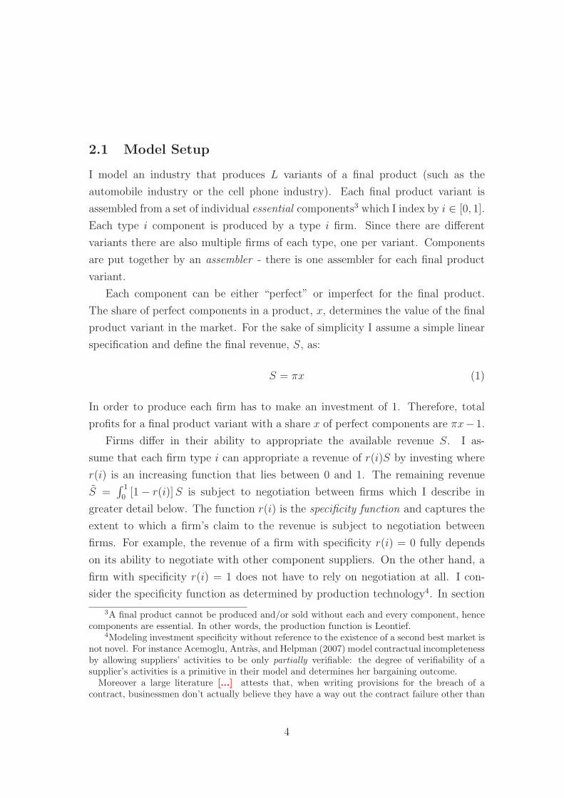
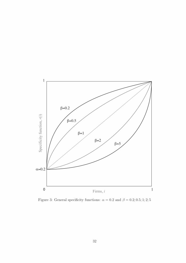
2.3.2 General specificity functions
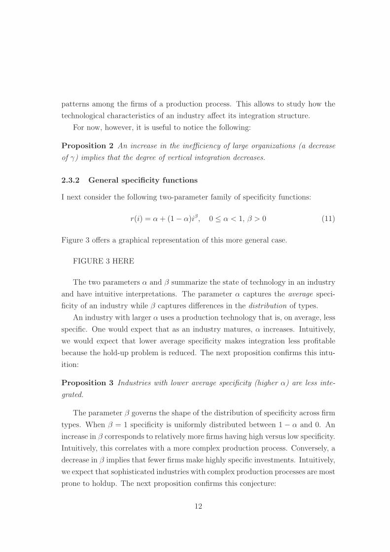
I next consider the following two-parameter family of specificity functions:
r(i) = α + (1 − α)iβ, 0 ≤ α < 1, β > 0 (11)
Figure 3 offers a graphical representation of this more general case.
FIGURE 3 HERE
The two parameters α and β summarize the state of technology in an industry
and have intuitive interpretations. The parameter α captures the average speci-
ficity of an industry while β captures differences in the distribution of types.
An industry with larger α uses a production technology that is, on average, less
specific. One would expect that as an industry matures, α increases. Intuitively,
we would expect that lower average specificity makes integration less profitable
because the hold-up problem is reduced. The next proposition confirms this intu-
ition:
Proposition 3 Industries with lower average specificity (higher α) are less inte-
grated.
The parameter β governs the shape of the distribution of specificity across firm
types. When β = 1 specificity is uniformly distributed between 1 − α and 0. An
increase in β corresponds to relatively more firms having high versus low specificity.
Intuitively, this correlates with a more complex production process. Conversely, a
decrease in β implies that fewer firms make highly specific investments. Intuitively,
we expect that sophisticated industries with complex production processes are most
prone to holdup. The next proposition confirms this conjecture:
12
Proposition 4 If production becomes more complex (β increases) vertical integra-
tion increases.
Finally, it can be easily shown that Proposition 2 holds in the extended model.10
3 Endogenous Investment
In the model introduced in the previous section integration is privately optimal
but socially wasteful. The total industry profit of both integrated and non-
integrated firms is greater under non-integration compared to integration, π− 1 >
π (1 − N∗ + γN∗)−1. This is because integrated firms are less flexible and produce
more imperfect components. Integration per se only allows the assembler to cap-
ture a disproportionate share of the appropriable revenue and hence is equivalent
to a welfare-neutral redistribution.
However, by fixing the level of investment at 1 for all firms my model shuts
down one potentially important channel through which integration might actually
increase welfare. Intuitively, integrated firms can shield their investment better
from expropriation. Since integrated firms make the most specific investments
within an industry this might increase the willingness of the integrated company
to invest in production.
The social planner might therefore allow integration because it may give rise
to a socially preferable second-best equilibrium.
I endogenize the level of investment using a highly simplified version of the
basic model:
1. There are two types of firms only: half have completely specific investment
(r = 0), half have not at all specific investment (r = 1)
2. Firms can invest either 1 or 2 units of capital.
10It suffices to show that the derivative of (16) with respect to γ is positive. Indeed it is:
∂(16)
∂γ=
N(
Nβ(1 − α) + α + β(
1 + 2(1 − α)(1 − 2N + N2))
)
(1 − α)β(
1 − (1 − γ)N)2
> 0 ∀N > 0
13
3. The productivity of investment is π1 (or π1(1−N + γN)) if a firm invests 1,
while it is π2 (or π2(1 − N + γN)) if it invests 2, with π1 > π2 > 1
4. The productivities are sufficiently large but not too close one another (in
particular 2γ
< π1 < 73
and π1
2+ 1
2γ< π2 < π1
2+ 1)
Under the above assumptions the following holds:
Proposition 5 If γ is close enough to 1, then the following statements are true:
1. Under non integration high specificity firms invest 1 and low specificity firms
invest 2
2. The equilibrium is characterized by full integration (N∗ = 1)
3. In equilibrium the assembler invests 2 in all the divisions of the vertically
integrated firm
4. The total surplus produced is greater in the integrated equilibrium than under
non integration
The proposition above demonstrates that integration is not necessarily detri-
mental to welfare. In fact, by providing a protection against revenue expropriation,
integration can provide greater incentives to invest. In some cases, as shown in the
proposition, this is sufficient to overcome the efficiency loss caused by integration
and, consequently, integration can enhance welfare.
4 Applications and predictions of the model
Vertical integration has generally diminished over the last few decades (Rajan and
Wulf (2006), Brynjolfsson, Malone, Gurbaxani, and Kambil (1994)). Companies
have increasingly outsourced activities that were previously carried out inside the
firm (Spencer (2005), Hummels, Ishii, and Yi (2001)). Firms have gained flexibility
by purchasing intermediate components on the market rather than producing them
inside the firm. These trends were accompanied by a deepening of financial markets
and rapid growth in some developing countries.
14
In the following I use the model developed in section 2.3.2 to provide a unified
interpretation of a variety of inter-related phenomena.
Applied research and process innovation. For a given industry, advances
in applied research and process innovation improve the efficiency and efficacy of
existing technologies. This kind of innovation tend to give physical capital gen-
erally more flexible production capabilities: technological advances have made
machinery both more responsive to production timing needs and market demand
rhythms as well as normally able to produce less standardized goods with a compa-
rable amount of invested capital. As an example, consider the diffusion of robotics
and just-in-time plant management techniques: Nemetz and Fry (1988) point out
that such flexible manufacturing technologies favor organizational forms with a
narrow span of control, a lower number of vertical layers and a more decentralized
decision making process as compared to mass production technology organizations.
In the context of my model these changes are equivalent to an increase of α, the
general state of technology. In fact, such advancements reduce the costs associated
to a certain technology and slowly help it spread throughout the economy, making
it increasingly standard. This, in turn, implies that investment in such technol-
ogy becomes less specific. In addition, it is likely that, if any, applied research
decreases β: in fact, those production stages which are less complex and tend to
be less specific are more likely to become standard first. Both these effects imply
a decrease of the optimal degree of vertical integration. This explains some impor-
tant aspects of the general trend in industries like automobiles: in such industries
the introduction of more flexible production techniques has made it convenient the
outsourcing of many activities to specialized firms. These in fact are now able to
provide different products for different customers with a comparable amount of
investment.
Human capital. It is well known that today’s economies are characterized by
a high and increasing level of human capital11. As modern economies move toward
services and knowledge intensive sectors, human capital has gained importance as
arguably the major factor of production. Now, human capital is by nature much
11As Gary S. Becker puts it, “Human capital is increasingly important in modern economies.Skills and knowledge are highly valuable in more high-tech economies [...]” (from a public con-ference in Milan, the 22nd of June 1998).
15
more flexible than physical capital and, to a great extent, it is non relation-specific.
In fact, if it is true that it is probably difficult for a nuclear physicist to become a
financial broker overnight, it is certainly true that the personal histories of many
businessmen, professionals and scientists demonstrate how easily human capital
transfers across and within single firms and sectors of the economy. Therefore an
investment in human capital tends to be less specific to the relationship and to
generate less quasi rents than an investment in physical capital. In terms of the
model a generalized increase of the ratio of human to physical capital is equivalent
to a rise in α as it touches, at least to some extent, all the industries and all the
production stages of an industry. This leads to a decrease of the optimal degree
of vertical integration. However, it is not clear how the rise in relative importance
of human vs. physical capital affects β making it hard to say what the final effect
is. MacDonald (1985) finds that the use of vertical integration is more prevalent
in capital intensive industries while Hortacsu and Syverson (2007) document that,
within an industry, vertically integrated firms have a higher capital-to-labor ratio
than non integrated firms. These findings, which appear to be robust, suggest that
more human capital as compared to physical capital leads to less integration.
Financial markets. As pointed out by Rajan and Zingales (2001), another
reason for why physical capital is today less crucial than in the past is the huge
development of financial markets in the last decades which has made it much less
of a constraint the acquisition of machineries, the building of new plants and the
investment in equipment in general. In fact, various authors (Rajan and Zingales
(2001); Acemoglu, Johnson, and Mitton (2005)) have studied the relationship be-
tween vertical integration and the development of financial markets. The argument
behind such studies is that more efficient financial markets tend to reduce the hold
up problem and, a fortiori, the degree of vertical integration. The mere existence
of efficient credit markets -the argument goes- makes hold up threads less credi-
ble because they provide entrepreneurs with more easily accessible outside options.
For instance, if a partner threatens to withdraw from production, an efficient credit
market might well mean that the threatened partner is able -or at least have more
chances- to buy and/or build the machineries to internally produce the missing
component. In other words, “with capital easy to come by, alienable assets such as
plant and equipment have become less unique” (Rajan and Zingales (2001)). This
16
means that physical investment is less relation-specific as a consequence of more
efficient financial markets. Ideally, with perfect financial markets, no hold up may
be based on any asset which could be possibly borrowed. In terms of the model the
development of financial markets can be formalized as an increase of α. Moreover,
it is likely that efficient credit markets are worth most to firms producing complex
products which have very specific investments. Thus, if any, β should decrease as
financial markets become more efficient. Which means that the degree of vertical
integration tends to diminish as a consequence of financial development.
Industries comparison. The model predicts that complex products requiring
high-tech and sophisticated machinery are produced in industries whose structure
tends to be more vertically integrated. In fact, one can interpret the parameter
β as a proxy for technology intensity or complexity. A sophisticated or complex
final product involves a relatively large number of sophisticated intermediate prod-
ucts which require investment in highly specific machinery: this corresponds to a
high β (see Figure 3). A relatively standard product, on the contrary, involves
relatively fewer complex stages of production, with less specific investments: this
corresponds to a small β. Thus, technology intensive products will be produced by
more integrated industries than standard products. Evidence of the above is very
neatly provided by Novak and Eppinger (2001) who explicitly test the hypothesis
that product complexity and vertical integration are complements. More evidence
has been provided by Wilson (1977) who finds that licensing is more attractive the
less complex the good involved is, and by Kogut and Zander (1993) whose results
show that the probability of internalization is lower the more codifiable, teachable,
and the less complex the technology is.
North-South differences. As a consequence of the previous point, poor
countries, producing less technology intensive products than rich countries, tend
to have a lower number of vertical conglomerates. This is consistent with the
observation that the economies of poor countries are generally characterized by
household-style, non integrated firms.
USA vs. Japanese keiretsu. Various authors (Spencer and Qiu (2001);
Qiu and Spencer (2002)) have studied the case of the Japanese keiretsu and the
reluctance of such conglomerates to import auto parts from abroad. They stress
17
the fact that the Japanese import only parts of limited technological content, such
as seat covers. The model presented in this paper predicts this phenomenon. In
fact, the model gives a rationale for why the most complex and technology intensive
parts of a production process should be produced internally. Those parts, in fact,
are the ones which require the most specific investments and which therefore will
be carried out by the vertical integration. Which, in the context of the Japanese
automobile industry, is the keiretsu itself. Only the less sophisticated parts are
produced by non integrated firms and therefore can be imported.
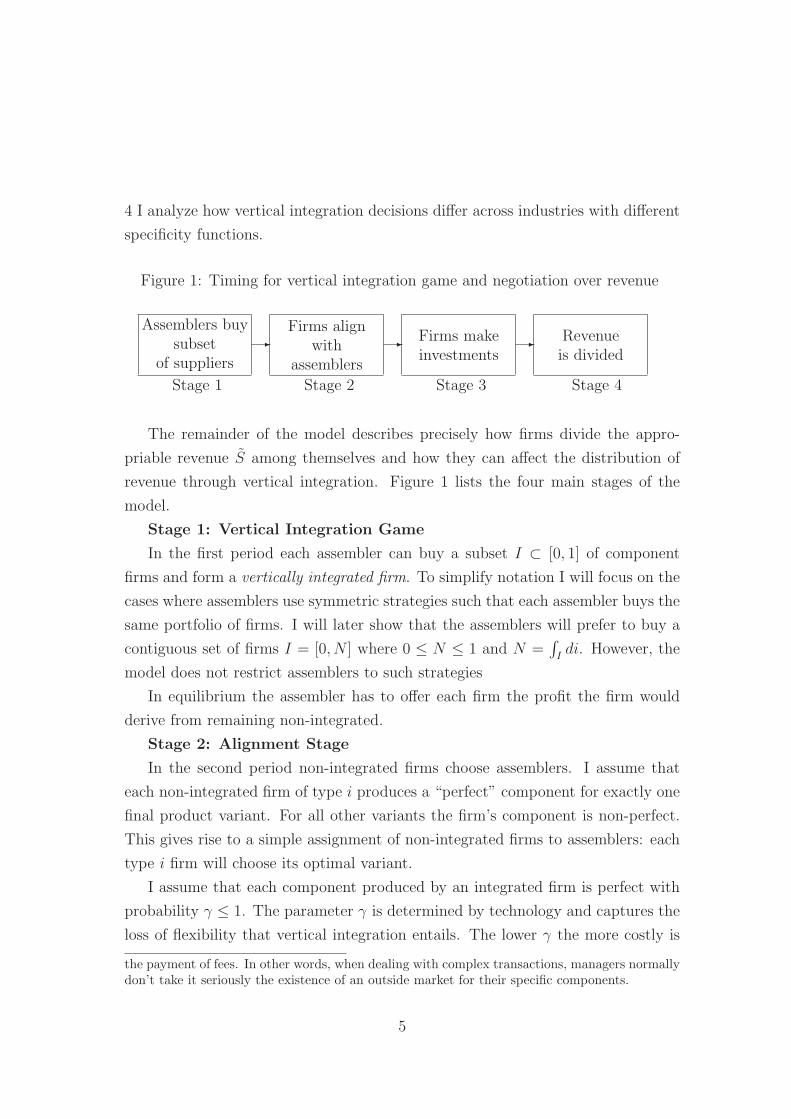
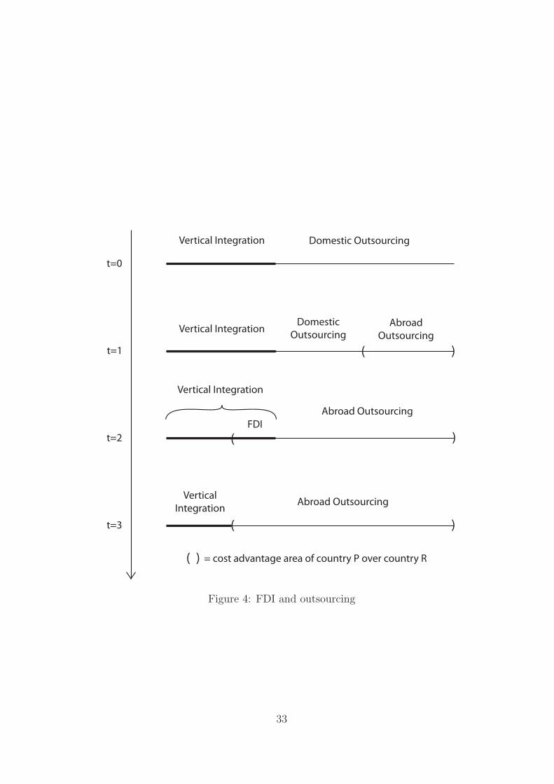
Trade patterns. Some authors (Vernon (1966); Antras (2005)) have explained
the pattern which leads firms to produce certain parts first internally, then in
regime of FDI and finally outsourcing them to less developed countries. In partic-
ular, Antras (2005) gives a Property Rights interpretation of such pattern. The
model presented here is able to explain the pattern quite naturally by assuming
that a) there is a (labor) cost advantage of poor countries (P); that b) rich coun-
tries (R) have a technological supremacy which reduces over time as poor countries
develop; and that c) there is technological progress12 and product standardization
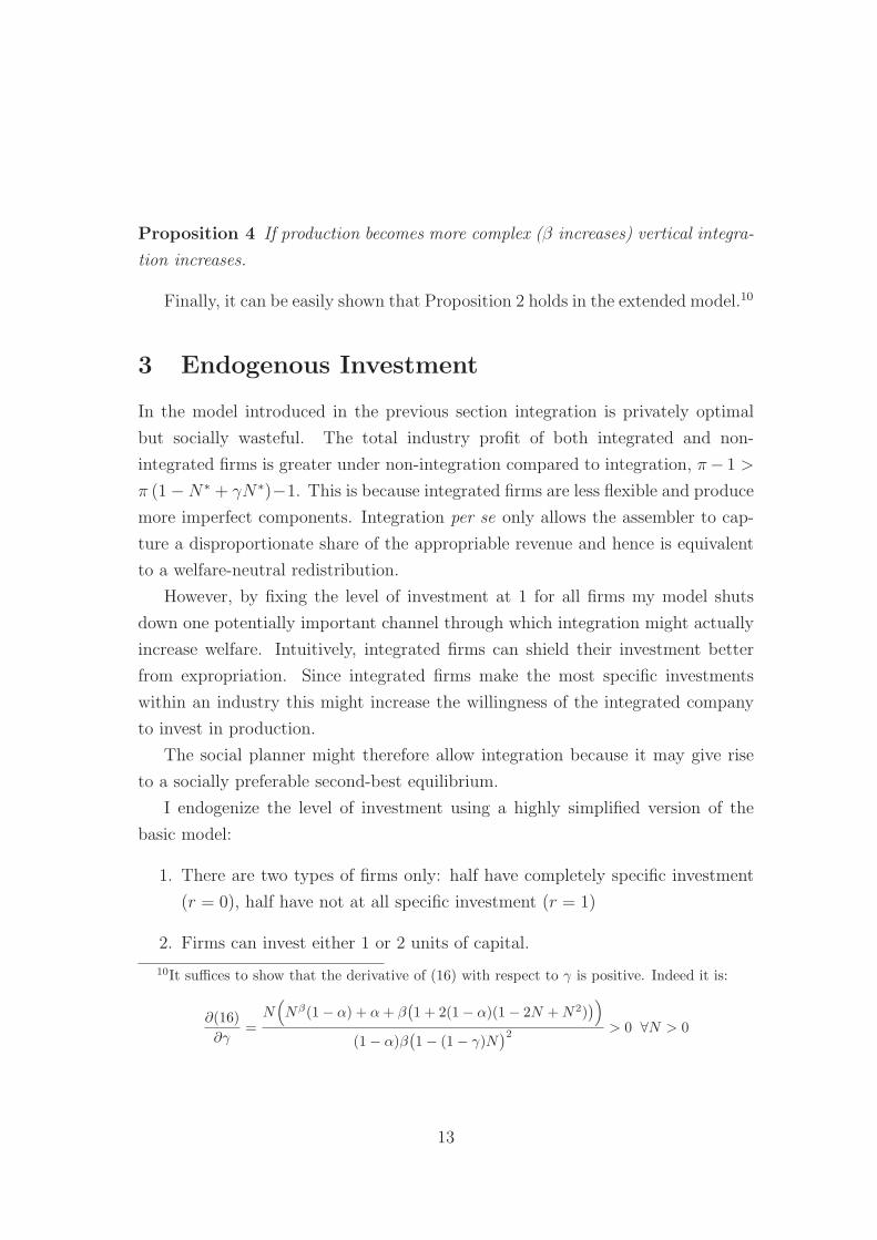
over time. Suppose there are four periods.
t=0 The product is invented in R, P has no skills and cannot produce. All produc-
tion is in R and, given technology, the optimal degree of vertical integration
is V I. The rest is produced in regime of domestic outsourcing
t=1 P develops, it becomes able to produce some parts: the firm in R buys some
standard pieces from P in foreign outsourcing regime
t=2 P develops further, it can produce more complex parts which are critical
to the firm: these are produced in regime of FDI with the firm operating
directly in P
t=3 Technology evolves: (some of) the parts produced in FDI are sufficiently
standard -no longer critical- to be bough outside the firm, hence the move
from FDI to outsourcing
12In particular applied research and process innovation may reduce the importance of hightech, critical inputs with the age or maturity of the final good as in Antras (2005).
18
The pattern just described is only a plausible example but many other patterns
could arise. It is depicted in Figure 3 where the horizontal lines represent the
spectrum of firms aligned from the most specific to the least, with the vertical
integration in bold.
FIGURE 4 HERE
Basic research. From the previous points it may seem that technological
progress will eventually undo vertical integration. Even though such perspective
is intriguing, vertically integrated firms are likely to endure. In fact, scientific
progress and basic research keep “creating” new products which, at least at the
beginning of their life cycle, are usually complex and non standard (robotic ma-
chines, hydrogen cars, new pharmaceuticals, etc.). Such products normally require
very specific investments before the technologies involved become standard and the
industry mature. This means that, as long as new discoveries are made, there will
still be a “demand for” vertical integration.
5 Conclusion
I have presented a theory of vertical integration which explains why and to what
extent firms in an industry become vertically integrated. The perspective of this
paper emphasizes the bargaining problem associated to the vertical integration
decision rather then the incentives to invest. As such, it is not mutually exclusive
with the prevalent Grossman-Hart-Moore perspective but rather complementary.
My model predicts that integration is the privately optimal response of a subset
of firms to their investments being appropriated by other firms with less specific
investments. Integration is viewed here as a means to gain bargaining power with
respect to non integrated firms. The context is a relationship between an assembler
and several suppliers which concur to the production of a final good and which
expropriate each other’s revenue because their investments are specific to the re-
lationship. Integration is the ex-ante optimal response of an assembler who has
to decide how much production to do in-house. He optimally integrates the firms
more exposed to expropriation in the ex-post bargaining problem: by merging
19
them into a larger organization he gains bargaining power and enjoys a dispropor-
tionately larger share of the total appropriable revenue. This happens at the cost
of foregone flexibility: the assembler is no longer able to choose the best suppliers
for its final good.
This paper views vertical integration as an optimal economizing strategy in the
presence of asymmetric exposure to expropriation: firms which are more exposed to
expropriation benefit the most from the increased power provided by integration.
As Williamson pointed out, there is, in the real world, a continuum of specificity
degrees: as the degree of specificity increases, the market becomes less and less
feasible for some firms and integration becomes a better response to the hold-up
problem. Coherent with a view which regards the market as the optimum, the
model displays a welfare loss in any equilibrium which involves integration.
However, the paper also considers the effect of integration on incentives and
demonstrates that there are conditions under which integration is indeed welfare
improving. In fact, by providing a shield against expropriation, integration im-
proves the incentive to invest of the assembler. In an extension of the model where
firms are allowed to vary the size of their investment it is shown that, under certain
conditions, the shield provided by integration leads to more investment and to a
higher welfare.
The paper also illustrates in which sense the technological development of the
several past decades might have impacted the organizational structure of firms
causing a wave of externalizations and a surge in outsourcing strategies. I ar-
gue that process innovation has made capital less specific over time reducing the
average degree of specificity of a given industry. This has made integration less
valuable over time determining the observed pattern of organizational structures.
Finally, the model offers a key to interpret the different propensity to vertically
integrate in different industries. I argue that when a majority of the stages of a
production process involve highly specific investments then it will be observed a
more vertically integrated organization of production and vice versa.
The model has a number of testable implications and provides an interesting
opportunity for the empirical researcher to further investigate the relationship
between specific investment, technology and vertical integration.
20
References
Acemoglu, D., P. Aghion, R. Griffith, and F. Zilibotti (2004): “Vertical
Integration and Technology: Theory and Evidence,” NBER Working Paper.
Acemoglu, D., P. Antras, and E. Helpman (2007): “Contracts and tech-
nology Adoption,” American Economic Review, 97(3), 916–943.
Acemoglu, D., S. Johnson, and T. Mitton (2005): “Determinants of Vertical
Integration: Finance, Contracts and Regulation,” NBER Working Paper.
Antras, P. (2005): “Incomplete Contracts and the Product Cycle,” American
Economic Review, 95, 1054–1073.
Bajari, P., and S. Tadelis (2001): “Incentives versus Transaction Costs: A
Theory of Procurement Contracts,” The RAND Journal of Economics, 32(3),
387–407.
Brynjolfsson, E., T. Malone, V. Gurbaxani, and A. Kambil (1994):
“Does Information Technology Lead to Smaller Firms?,” Management Science,
40(12), 1628–1644.
Chemla, G. (2003): “Downstream Competition, Foreclosure, and Vertical Inte-
gration,” Journal of Economics & Management Strategy, 12, 261–289.
Christensen, C. M., M. Raynor, and M. Verlinden (2001): “Skate to
Where the Money Will Be,” Harvard Business Review, November, 72–81.
Coase, R. H. (1937): “The Nature of the Firm,” Economica, 4(16), 386–405,
New Series.
Commons, J. R. (1931): “Institutional Economics,” The American Economic
Review, 21(4), 648–657.
Grossman, G. M., and E. Helpman (2002): “Integration Versus Outsourcing
in Industry Equilibrium,” The Quarterly Journal of Economics, 117(1), 85–120.
(2005): “Outsourcing in a Global Economy,” Review of Economic Studies,
72, 135–159.
21
Grossman, S. J., and O. D. Hart (1986): “The Costs and Benefits of Own-
ership: A Theory of Vertical and Lateral Integration,” The Journal of Political
Economy, 94(4), 691–719.
Hart, O., and J. Moore (1990): “Property Rights and the Nature of the Firm,”
The Journal of Political Economy, 98(6), 1119–1158.
Hart, O., and J. Tirole (1990): “Vertical Integration and Market Foreclosure,”
Brookings Papers on Economic Activity. Microeconomics, 1990(2), 205–286.
Head, K., J. Ries, and B. J. Spencer (2004): “Vertical Networks and US
Auto Parts Exports: Is Japan Different?,” Journal of Economics & Management
Strategy, 13(1), 37–67.
Holmstrom, B., and J. Roberts (1998): “The Boundaries of the Firm Revis-
ited,” The Journal of Economic Perspectives, 12(4), 73–94.
Hortacsu, A., and C. Syverson (2007): “Vertical Integration and Production:
Some Plant-Level Evidence,” Working Paper.
Hummels, D., J. Ishii, and K.-M. Yi (2001): “The nature and growth of
vertical specialization in world trade,” Journal of International Economics, 54,
75–96.
Jensen, M. C., and W. H. Meckling (1976): “Theory of the Firm: Manage-
rial Behavior, Agency Costs and Ownership Structure,” Journal of Financial
Economics, 3, 305–360.
Jensen, M. C., and K. J. Murphy (1990): “Performance Pay and Top-
Management Incentives,” The Journal of Political Economy, 98(2), 25–264.
Joskow, P. L. (1985): “Vertical integration and Long-Term Contracts: The Case
of Coal-Burning Electric Generating Plants,” The Journal of Law, Economics
& Organization, 1(1), 33–80.
Kalai, E. (1977): “Nonsymmetric Solutions and Replications of Two-Person Bar-
gaining,” International Journal of Game Theory, 6(3), 129–133.
22
Kemp, T. (2006): “Of Transactions and Transaction Costs: Uncertainty, Policy,
and the Process of Law in the Thought of Commons and Williamson,” Journal
of Economic Issues, XL, 45–58.
Kogut, B., and U. Zander (1993): “Knowledge of the Firm and the Evo-
lutionary Theory of the Multinational Corporation,” Journal of International
Business Studies, 24(4), 625–645.
Kranton, R. E., and D. F. Minehart (2002): “Vertical Foreclosure and
Specific Investments,” Working Paper.
Langlois, R. N. (1992): “External Economies and Economic Progress: The
Case of the Microcomputer Industry,” The Business History Review, 66(1), 1–
50, High-Technology Industries.
MacDonald, J. M. (1985): “Market Exchange or Vertical Integration: An Em-
pirical Analysis,” The Review of Economics and Statistics, 67(2), 327–331.
Magretta, J. (1998): “The Power of Virtual Integration: and Interview with
Dell Computer’s Michael Dell,” Harvard Business Review, 75, 72–84.
Masten, S. E. (1984): “The Organization of Production: Evidence from the
Aerospace Industry,” Journal of Law and Economics, 27(2), 403–417.
McLaren, J. (2000): “”Globalization and Vertical Structure”,” The American
Economic Review, 90(5), 1239–1254.
Nemetz, P. L., and L. W. Fry (1988): “Flexible Manufacturing Organizations:
Implications for Strategy Formulation and Organization Design,” OMEGA
Academy of Management Review, 13(4), 627–638.
Novak, S., and S. D. Eppinger (2001): “Sourcing by Design: Product Complex
and the Supply Chain,” Management Science, 47(1), 189–204.
Qiu, L. D., and B. J. Spencer (2002): “Keiretsu and relationship-specific
investment: implications for market-opening trade policy,” Journal of Interna-
tiona Economics, 58, 49–79.
23
Rajan, R. G., and J. Wulf (2006): “The Flattening of the Firm: Evidence from
Panel Data on the Changing Nature of Corporation Hierarchies,” The Review
of Economics and Statistics, 88(4), 759–773.
Rajan, R. G., and L. Zingales (2001): “The Influence of the Financial Rev-
olution on the Nature of Firms,” The American Economic Review, 91(2), 206–
211, Papers and Proceedings of the Hundred Thirteenth Annual Meeting of the
American Economic Association.
Riordan, M. H., and O. E. Williamson (1985): “Asset Specificity and Eco-
nomic Organization,” International Journal of Industrial Organization, 3, 365–
378.
Salinger, M. A. (1988): “Vertical Mergers and Market Foreclosure,” Quarterly
Journal of Economics, 103(2), 345–356.
Spencer, B. J. (2005): “International outsourcing and incomplete contracts,”
Canadian Journal of Economics, 38(4), 1107–1135.
Spencer, B. J., and L. D. Qiu (2001): “Keiretsu and Relationship-Specific
Investment: A Barrier to Trade?,” International Economic Review, 42(4), 871–
901.
Vernon, R. (1966): “International Investment and International Trade in the
Product Cycle,” The Quarterly Journal of Economics, 80(2), 190–207.
Williamson, O. E. (1979): “Transaction-Cost Economics: The Governance of
contractual Relations,” Journal of Law and Economics, 22(2), 233–261.
(1981): “The Economics of Organization: The Transaction Cost Ap-
proach,” The American Journal of Sociology, 87(3), 548–577.
(1985): The Economic Institutions of Capitalism. Free Press.
(2002): “The Theory of the Firm as Governance Structure: From Choice
to Contract,” The Journal of Economic Perspectives, 16(3), 171–195.
24
Wilson, R. W. (1977): “The Effect of Technological Environment and Product
Rivalry on R&D Effort and Licensing of Inventions,” The Review of Economics
and Statistics, 59(2), 171–178.
25
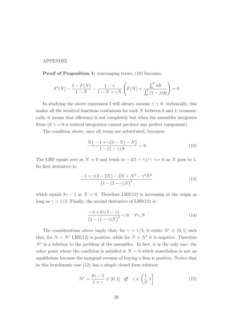
APPENDIX
Proof of Proposition 1: rearranging terms, (10) becomes:
F ′(N) −1 − F (N)
1 − N−
1 − γ
1 − N + γN
(
F (N) +
∫ N
0idi
∫ 1
0(1 − j)dj
)
= 0
In studying the above expression I will always assume γ > 0: technically, this
makes all the involved functions continuous for each N between 0 and 1; economi-
cally, it means that efficiency is not completely lost when the assembler integrates
firms (if γ = 0 a vertical integration cannot produce any perfect component).
The condition above, once all terms are substituted, becomes:
N(
− 1 + γ(3 − N) − N)
1 − (1 − γ)N= 0 (12)
The LHS equals zero at N = 0 and tends to −2(1 − γ)/γ <= 0 as N goes to 1.
Its first derivative is:
−1 + γ(3 − 2N) − 2N + N2 − γ2N2
(
1 − (1 − γ)N)2 (13)
which equals 3γ − 1 at N = 0. Therefore LHS(12) is increasing at the origin as
long as γ > 1/3. Finally, the second derivative of LHS(12) is:
−4 + 6γ(1 − γ)(
1 − (1 − γ)N)3 < 0 ∀γ,N (14)
The considerations above imply that, for γ > 1/3, it exists N∗ ∈ (0, 1] such
that, for N < N∗ LHS(12) is positive, while for N > N∗ it is negative. Therefore
N∗ is a solution to the problem of the assembler. In fact, it is the only one: the
other point where the condition is satisfied is N = 0 which nonetheless is not an
equilibrium because the marginal revenue of buying a firm is positive. Notice that
in this benchmark case (12) has a simple closed form solution:
N∗ =3γ − 1
1 + γ∈ (0, 1] iff γ ∈
(
1
3, 1
]
(15)
26
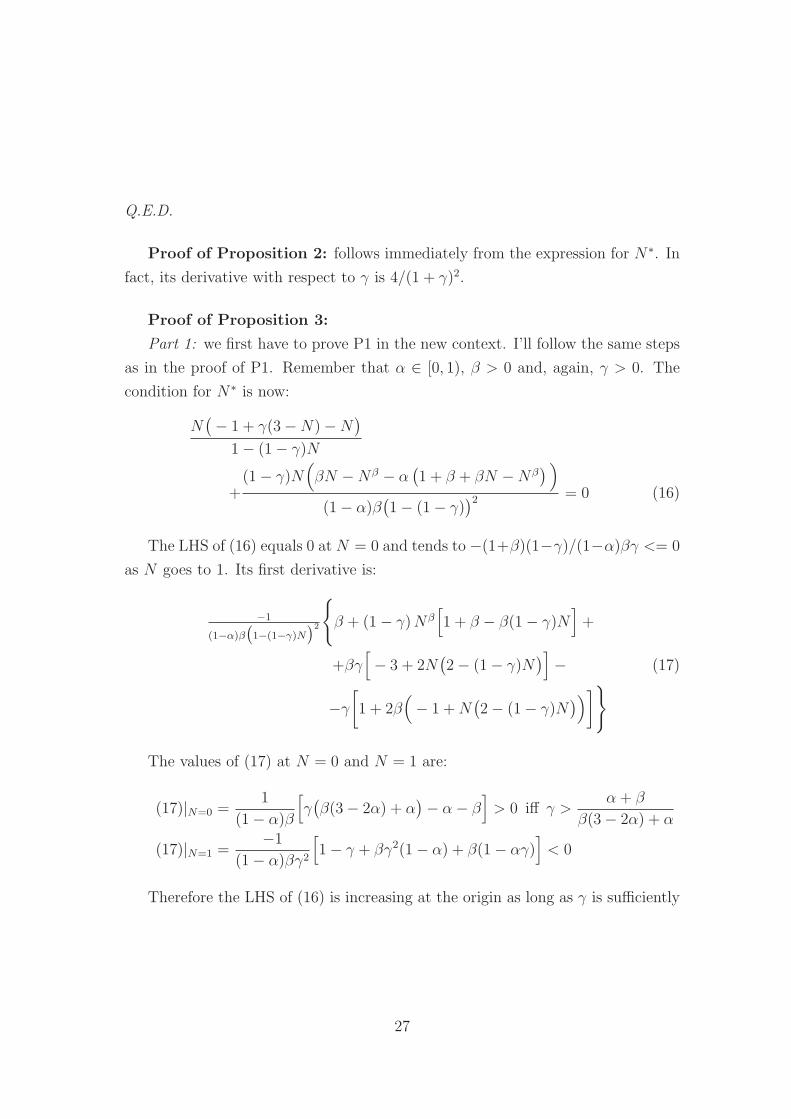
Q.E.D.
Proof of Proposition 2: follows immediately from the expression for N∗. In
fact, its derivative with respect to γ is 4/(1 + γ)2.
Proof of Proposition 3:
Part 1: we first have to prove P1 in the new context. I’ll follow the same steps
as in the proof of P1. Remember that α ∈ [0, 1), β > 0 and, again, γ > 0. The
condition for N∗ is now:
N(
− 1 + γ(3 − N) − N)
1 − (1 − γ)N
+(1 − γ)N
(
βN − Nβ − α(
1 + β + βN − Nβ)
)
(1 − α)β(
1 − (1 − γ))2 = 0 (16)
The LHS of (16) equals 0 at N = 0 and tends to −(1+β)(1−γ)/(1−α)βγ <= 0
as N goes to 1. Its first derivative is:
−1
(1−α)β(
1−(1−γ)N)2
{
β + (1 − γ) Nβ[
1 + β − β(1 − γ)N]
+
+βγ[
− 3 + 2N(
2 − (1 − γ)N)
]
− (17)
−γ
[
1 + 2β(
− 1 + N(
2 − (1 − γ)N)
)
]
}
The values of (17) at N = 0 and N = 1 are:
(17)|N=0 =1
(1 − α)β
[
γ(
β(3 − 2α) + α)
− α − β]
> 0 iff γ >α + β
β(3 − 2α) + α
(17)|N=1 =−1
(1 − α)βγ2
[
1 − γ + βγ2(1 − α) + β(1 − αγ)]
< 0
Therefore the LHS of (16) is increasing at the origin as long as γ is sufficiently
27
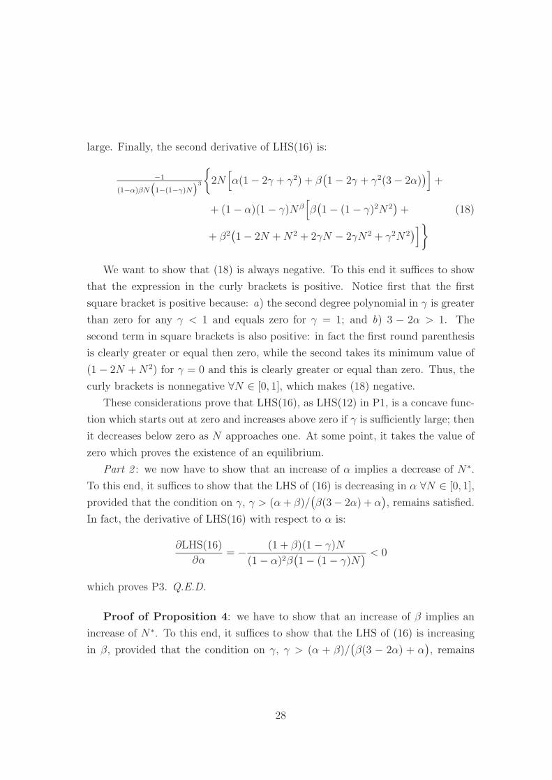
large. Finally, the second derivative of LHS(16) is:
−1
(1−α)βN
(
1−(1−γ)N)3
{
2N[
α(1 − 2γ + γ2) + β(
1 − 2γ + γ2(3 − 2α))
]
+
+ (1 − α)(1 − γ)Nβ[
β(
1 − (1 − γ)2N2)
+ (18)
+ β2(
1 − 2N + N2 + 2γN − 2γN2 + γ2N2)
]
}
We want to show that (18) is always negative. To this end it suffices to show
that the expression in the curly brackets is positive. Notice first that the first
square bracket is positive because: a) the second degree polynomial in γ is greater
than zero for any γ < 1 and equals zero for γ = 1; and b) 3 − 2α > 1. The
second term in square brackets is also positive: in fact the first round parenthesis
is clearly greater or equal then zero, while the second takes its minimum value of
(1 − 2N + N2) for γ = 0 and this is clearly greater or equal than zero. Thus, the
curly brackets is nonnegative ∀N ∈ [0, 1], which makes (18) negative.
These considerations prove that LHS(16), as LHS(12) in P1, is a concave func-
tion which starts out at zero and increases above zero if γ is sufficiently large; then
it decreases below zero as N approaches one. At some point, it takes the value of
zero which proves the existence of an equilibrium.
Part 2 : we now have to show that an increase of α implies a decrease of N∗.
To this end, it suffices to show that the LHS of (16) is decreasing in α ∀N ∈ [0, 1],
provided that the condition on γ, γ > (α + β)/(
β(3− 2α) + α)
, remains satisfied.
In fact, the derivative of LHS(16) with respect to α is:
∂LHS(16)
∂α= −
(1 + β)(1 − γ)N
(1 − α)2β(
1 − (1 − γ)N) < 0
which proves P3. Q.E.D.
Proof of Proposition 4: we have to show that an increase of β implies an
increase of N∗. To this end, it suffices to show that the LHS of (16) is increasing
in β, provided that the condition on γ, γ > (α + β)/(
β(3 − 2α) + α)
, remains
28
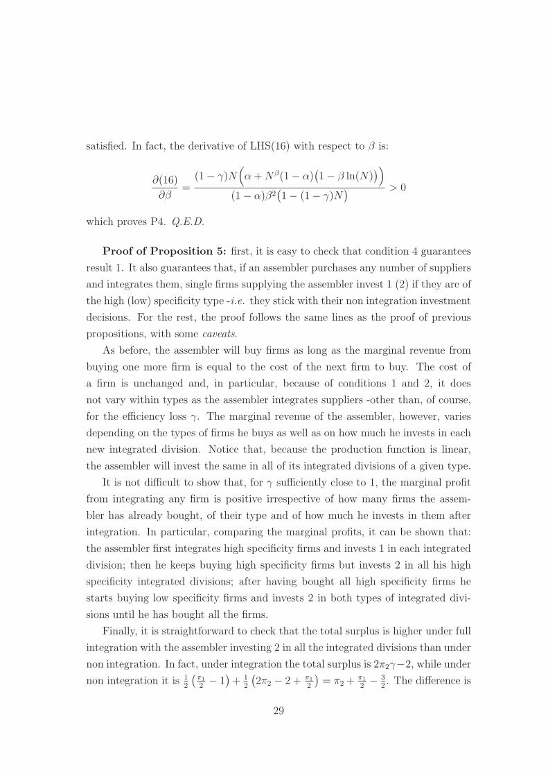
satisfied. In fact, the derivative of LHS(16) with respect to β is:
∂(16)
∂β=
(1 − γ)N(
α + Nβ(1 − α)(
1 − β ln(N))
)
(1 − α)β2(
1 − (1 − γ)N) > 0
which proves P4. Q.E.D.
Proof of Proposition 5: first, it is easy to check that condition 4 guarantees
result 1. It also guarantees that, if an assembler purchases any number of suppliers
and integrates them, single firms supplying the assembler invest 1 (2) if they are of
the high (low) specificity type -i.e. they stick with their non integration investment
decisions. For the rest, the proof follows the same lines as the proof of previous
propositions, with some caveats.
As before, the assembler will buy firms as long as the marginal revenue from
buying one more firm is equal to the cost of the next firm to buy. The cost of
a firm is unchanged and, in particular, because of conditions 1 and 2, it does
not vary within types as the assembler integrates suppliers -other than, of course,
for the efficiency loss γ. The marginal revenue of the assembler, however, varies
depending on the types of firms he buys as well as on how much he invests in each
new integrated division. Notice that, because the production function is linear,
the assembler will invest the same in all of its integrated divisions of a given type.
It is not difficult to show that, for γ sufficiently close to 1, the marginal profit
from integrating any firm is positive irrespective of how many firms the assem-
bler has already bought, of their type and of how much he invests in them after
integration. In particular, comparing the marginal profits, it can be shown that:
the assembler first integrates high specificity firms and invests 1 in each integrated
division; then he keeps buying high specificity firms but invests 2 in all his high
specificity integrated divisions; after having bought all high specificity firms he
starts buying low specificity firms and invests 2 in both types of integrated divi-
sions until he has bought all the firms.
Finally, it is straightforward to check that the total surplus is higher under full
integration with the assembler investing 2 in all the integrated divisions than under
non integration. In fact, under integration the total surplus is 2π2γ−2, while under
non integration it is 12
(
π1
2− 1)
+ 12
(
2π2 − 2 + π1
2
)
= π2 + π1
2− 3
2. The difference is
29
(2γ − 1) π2 −π1
2− 1
2, which is clearly positive under the above conditions. Q.E.D.
30
1
10 N’
j
k
k
j
Firms
Shar
e of
tota
l re
ven
ue
F(N)
Figure 2: F (N), Bargaining Power and Revenue Shares
31
1
1
α=0.2
0
β=0.2
β=0.5
β=1
β=2β=5
Firms, i
Sp
ecif
icit
y f
un
ctio
n, r(i)
Figure 3: General specificity functions: α = 0.2 and β = 0.2; 0.5; 1; 2; 5
32
(
(
( (
(
(
( ) = cost advantage area of country P over country R
Domestic Outsourcing
Domestic
OutsourcingAbroad
Outsourcing
Abroad Outsourcing
FDI
Vertical Integration
Vertical Integration
Vertical Integration
Vertical
IntegrationAbroad Outsourcing
t=0
t=1
t=2
t=3
Figure 4: FDI and outsourcing
33
Recommended