Term Structure Estimation in Markets with Infrequent Trading1
GONZALO CORTAZAR Pontificia Universidad Católica de Chile
EDUARDO S. SCHWARTZ University of California at Los Angeles
LORENZO F. NARANJO New York University
Term Structure Estimation in Markets with Infrequent Trading
ABSTRACT
There are two issues that are of central importance in term structure analysis. One is the modeling and estimation of the current term structure of spot rates. The second is the modeling and estimation of the dynamics of the term structure. These two issues have been addressed independently in the literature. The methods that have been proposed assume a sufficiently complete price data set and are generally implemented separately. However, there are serious problems when these methods are applied to markets with sparse bond prices.
We develop a method for jointly estimating the current term structure and its dynamics for markets with infrequent trading. We propose solving both issues by using a dynamic term structure model estimated from incomplete panel data. To achieve this, we modify the standard Kalman filter approach to deal with the missing-observation problem. In this way, we can use historic price data in a dynamic model to estimate the current term structure. With this approach we are able to obtain an estimate of the current term structure even for days with an arbitrary low number of price observations.
The proposed methodology can be applied to a broad class of continuous-time term-structure models with any number of stochastic factors. To show the implementation of the approach, we estimate a three-factor generalized Vasicek model using Chilean government bond price data. The approach, however, may be used in any market with infrequent trading, a common characteristic of many emerging markets.

2
1. Introduction
There are two issues that are of central importance in term structure analysis. One is the modeling and estimation of the current term structure of spot rates, which is essential for valuing and hedging cash flows that are linearly related to the discount function. The second is the modeling and estimation of the dynamics of the term structure, which is required for valuing and hedging cash flows that are non-linear functions of the term structure (all types of options). These two issues have been addressed independently in the literature.
For current term-structure estimation, most authors have proposed parametric and nonparametric methods for fitting curves to current bond prices (or yields) without regard to past prices. McCulloch (1971, 1975), Vasicek and Fong (1982), and Fisher, Nychka and Zervos (1994), among others, use spline curve-fitting methods to estimate the current term structure. Nelson and Siegel (1987), and Svensson (1994) use parsimonious representations of the yield curve, limiting the number of parameters and giving more stability to the term structure.
For the modeling of the term structure dynamics the main concern is the movement of the term structure across time. To address this issue one alternative is to model the stochastic movement of the spot rate and then to use no-arbitrage arguments to infer the dynamics of the term structure. Examples of this approach include one-factor mean-reverting models [Vasicek (1977)], two-factor models [Brennan and Schwartz (1979)], multifactor extensions of the Vasicek model [Langetieg (1980)], single-factor general equilibrium models [Cox, Ingersoll and Ross (1985)] and multi-factor extensions of the CIR model [Duffie and Kan (1996)], among many others. Another approach is to use the whole current term structure as the input to the model and no-arbitrage arguments to infer its stochastic movement [Ho and Lee (1986), Heath, Jarrow and Morton (1992)]. Even though these type of models use all the information contained in the current term structure they are more difficult to calibrate.
Once a dynamic model of interest rates is proposed, the estimation method that will be used must be chosen. One possibility is to estimate the model using a time-series of bond prices [Chan, Karolyi, Longstaff, and Sanders (1992), Broze, Scaillet, and Zakoian (1995), Brenner, Harjes, and Kroner (1996), Nowman

3
(1997, 1998), Andersen and Lund (1997)]. Alternatively, state variables and parameters may be estimated from a panel of bond prices with different maturities [Chen and Scott (1993), Pearson and Sun (1994), and Duffie and Singleton (1997)].
Even though there are obvious benefits of calibrating a model using a panel with a large number of price observations, the richer the data set, the larger the estimated measurement errors. These errors arise from the inability of a model with a limited number of factors to perfectly explain a large number of contemporaneous prices. A powerful and widely used methodology to optimally estimate unobservable state variables from a noisy panel-data is the Kalman filter. Recent applications of this methodology to dynamic models of interest rates include Lund (1994, 1997), Duan and Simonato (1995), Ball and Torous (1996), Geyer and Pichler (1998), Babbs and Nowman (2001), and Chen and Scott (2003). The advantage of using the Kalman filter on a panel-data is that it jointly uses all present and past price information. Maximum likelihood methods can then be used to estimate the parameters of the model.
Both type of methods proposed in the literature, curve-fitting for estimating the current term structure and Kalman filtering for dynamic models, have been successfully applied to markets for which there is a sufficiently complete price data-set. However, there are serious problems when these methods are used in markets with sparse bond price data. For example, traditional curve-fitting methods render unreliable estimates of the current term structure for days without a sufficient number of observations or without short or long-term bond prices. In addition, a typical Kalman filter implementation assumes a complete panel of bond prices (or yields), which becomes problematic if there is a substantial number of missing observations as is the case in many emerging markets.
In this article we develop and implement a method for jointly estimating the current term structure and its dynamics in markets with infrequent trading. We propose solving both issues by using a dynamic term structure model estimated from incomplete panel data. To achieve this, we modify the standard Kalman filter approach to deal with the missing-observation problem. We can then use historical price data and a dynamic model to estimate the current term structure. With this approach, we are able to obtain an estimate of the current term structure even for days with an arbitrary low number of price observations.

4
The proposed methodology can be applied to a broad class of continuous-time term-structure models with any number of stochastic factors. To show the implementation of the approach for an emerging market with infrequent trading, we estimate a three-factor generalized-Vasicek model using Chilean government bond price data. The approach, however, may be used in any market with infrequent trading as is the case in many emerging markets.
The next section explains the shortcomings of static term-structure estimation methods when there is sparse data. In Section 3 we present the generalized Vasicek model that will be used for illustrating our methodology. Section 4 presents the standard Kalman filter method and shows how it can be used in an incomplete panel-data setting. Section 5 presents empirical results of applying the methodology to the Chilean government bond market and Section 6 concludes.
2. Shortcomings of Static Term-Structure Estimation Markets with Infrequent Trading
Term structure estimation has been traditionally implemented with static models that only use current bond prices (or yields), without regard to past information. Some methods, like Nelson and Siegel (1987) and Svensson (1994), assume a parametric functional form for the forward rates2. Other methods, for example McCulloch (1971, 1975), and Fisher, Nychka and Zervos (1994), use non-parametric spline-based interpolation methods to calculate the term structure. Empirical evidence shows that in well developed markets, where numerous bonds are traded every day for different maturities, these static methods generate yield curves that accurately fit current bond transactions [Bliss (1996)].
There are, however, other features besides goodness-of-fit to observed prices that are desirable in a term-structure model, such as the time-series stability of the term-structure curves obtained. This stability can be analyzed by observing the sequence of daily term-structure estimations implied by the model. It might well be the case that the model fits very well existing bond prices (or yields), but it implies
2 See Appendix A for details on these methods.

5
large daily movements of yields for maturities that are not traded. This is not an issue for liquid markets, but as we shall see, is a serious problem for thin markets. One way of assessing the stability of the term-structure curves obtained is to compare the volatilities from the model with actual volatility from the data.
In markets with a complete cross-section of prices for each date, volatility of interest rates computed from the estimated term structures will closely match historical data and the stability of the model is not an issue. However, for sparse data sets in which at each date there are only a few different bond maturities traded, stability will become an important criteria for judging the reliability of the term structure estimation.
When the number of observed prices for a particular date is not sufficiently larger than the number of parameters to be estimated, any measurement error crucially affects the shape of the fitted curve. An extreme case is when the number of parameters to be estimated is larger than the number of observed prices; in this case there is an infinite number of curves that fit the observed prices. Figure 1 illustrates this extreme (but not uncommon in emerging markets) case of a date with fewer prices than model parameters by plotting two of the infinite term-structures that perfectly explain observed prices. This example is taken from one of the many dates in the Chilean government bond market with extremely thin trading. Curve-fitting methods clearly cannot be applied to dates with very low number of transactions.
A second problem of these static curve-fitting methods when used in markets with infrequent trading occurs when the prices for short or for long-term bonds are not available, even if the number observed prices is sufficient for the estimation. Curve-fitting methods provide reasonable estimates within the time range spanned by the available prices, but provide much less reliable estimates for extrapolations outside this range. In many emerging markets it is common that for some dates long-term bonds are not traded; but the need for a complete term-structure estimation for valuation and hedging purposes remains.
Figure 2 illustrates a 20-year term-structure estimate of the coupon-bond-yield in Chile for 10/06/1999, a date in which there are sufficient bond prices but the maturity of the longest bond traded was only 6 years. We use all pure-discount and

6
coupon bonds3 traded on that date to compute the implied pure-discount yield curve using the Svensson (1994) method. Once this curve is obtained we compute the yields of coupon bonds with maturities from 0.5 to 20 years priced using the implied pure-discount yield curve estimated earlier. This coupon-yield curve is then plotted in Figure 2 together with the yields of all market transactions on 10/06/1999 and on the day before.
From Figure 2 we can see that prices of traded bonds with similar maturities did not change much between both dates and that long-term bonds were traded only on the first day. Even though observed prices indicate that markets seem to have behaved similarly on both dates, the model estimates that the yield of a 19-year coupon bond changed by almost 1% in a day. The extrapolated 19-year yield is clearly inaccurate. Curve-fitting methods provide unstable estimates of long rates when no long-term bonds are traded.
Instability of term-structure estimates can be measured by comparing the volatility term-structure implied by the model with the empirical volatilities obtained from the time series of yields. It is well-known that the term structure of volatilities is downward sloping due to mean reversion in interest rates. This means that the volatility of long rates obtained form the model should be lower than the volatility of short rates.
Figure 3 plots the volatility of interest rates calculated from daily estimations of the term-structure in Chile between 1997 and 2001 using the Svensson (1994) method. It can be seen that this term-structure of volatilities is not consistent with mean reversion in interest rates: it implies very high volatilities for long-rates. Moreover, the Svensson volatility estimates are much higher than the empirical estimates obtained directly from bond prices, suggesting that missing observations induce unreliable rate estimates. Similar results are obtained when using other curve-fitting methods like Nelson and Siegel (1987).
3 The coupon bonds considered here are amortizing bonds paying semi-annually equal
coupons. These instruments are described in more detail in Section 5.

7
Bond Yields - 12/22/2000
0%
2%
4%
6%
8%
0 5 10 15 20Maturity (Years)
Yie
ld (%
)
Observed Bond Yields
N & S Method Bond Yields 1
N & S Method Bond Yields 2
Fig. 1. Two different estimations of yield curves from Chilean government inflation-protected discount and coupon bond data using the Nelson & Siegel method for
12/22/2000.
Fig. 2. Coupon bond yields for two consecutive dates (10/05/1999 and 10/06/1999) estimated from Chilean government inflation-protected discount and coupon bond
data using the Svensson (1994) method.
Bond Yields - 10/06/1999
0%
2%
4%
6%
8%
0 5 10 15 20Maturity (Years)
Yiel
d (%
)
Observed Bond Yields
Svensson Method Bond Yields
Previous Day Observed Bond Yields
Previous Day Svensson Method Bond Yields

8
Fig. 3. Empirical volatilities of interest rates in Chile and volatilities obtained from daily estimations of the term-structure between 1997 and 2001 using the Svensson
(1994) method.
3. The Generalized Vasicek Dynamic Term-Structure Model
As was shown in the previous section, traditional static term structure estimation only incorporates current bond price (or yield) observations, without regard to past information. When long-term bond prices are not available, the estimation of long-term interest rates becomes unreliable. Also, without a sufficient number of transactions an over-parameterization of traditional models can occur.
We propose to solve the problems of term-structure estimation in markets with infrequent trading by using also past price information to infer the current term structure. This requires a dynamic model of the stochastic behavior of interest rates to be able to mix current and past prices in a meaningful way.
Some dynamic models, in particular multifactor ones, use a limited number of unobservable factors to summarize the stochastic behavior of the whole yield curve in a way that is sufficiently accurate, but also tractable. These unobservable state variables, together with the model parameters, must be estimated using observable bond price information. In the following sections we present an estimation methodology, based in the Kalman filter, that may be successfully used to
Volatility Structure of Interest Rates (1997-2001)
0%
2%
4%
6%
8%
10%
12%
14%
1.5 3.5 5.5 7.5 9.5 11.5 13.5Maturity (Years)
Vola
tility
Svensson Method Volatility Structure
Empirical Volatility from Bond Yields

9
estimate the term structure in markets with infrequent trading. To illustrate our estimation methodology we will consider a generalized Vacisek model for the instantaneous risk free interest rate. Our methodology may be used, however, with other interest rate models such as a one factor CIR model [Cox, Ingersoll and Ross (1985)], a multifactor CIR model [Duffie and Kan (1996)] or general exponential-affine models [Dai and Singleton (2001)], among others.
A generalized Vasicek model is a multifactor mean-reverting Gaussian model of the instantaneous spot interest rate which extends Vasicek (1977). This generalized formulation goes back to Langetieg (1980), and is also analyzed in Babbs and Nowman (1999). It considers n stochastic mean-reverting factors represented by the vector tx , of dimension 1n× , that define the instantaneous interest rate tr :
t tr δ′= +1 x (1)
The vector of state variables tx is governed by the following stochastic
differential equation:
t t td dt d= − +x Kx Σ w (2)
where ( )idiag k=K and ( )idiag σ=Σ are n n× diagonal matrices with entries that are strictly positives constants and different. Also, tdw is a 1n× vector of
correlated Brownian motion increments such that:
( ) ( )t td d dt′ =w w Ω (3)
where the ( , )i j element of Ω is [1, 1]ijρ ∈ − , the instantaneous correlation of state
variables i and j . Under this specification, the state variables have the multivariate
normal distribution and each of them reverts to 0, at a mean reversion rate4 given by ik . Thus, according to equation (1) the instantaneous interest rate reverts to a long
term value given by the constant δ . Note that this is a canonical model in the sense
4 In a mean reverting model, every perturbation is on average reduced by half in log(2) / ik units of time.

10
that it contains the minimum number of parameters that can be econometrically identified (see Dai and Singleton, 2001)5.
By assuming constant risk premiums6 λ , the risk-adjusted process for the vector of the state variables is:
( )t t td dt d= − + +x λ Kx Σ w (4)
where λ is a 1n× vector of constants.
Applying standard no-arbitrage arguments, we obtain the value of a pure-discount bond ( , )tP tx :
( )( , ) exp ( ) ( )t tP vτ τ τ′= +x u x (5)
where
1 exp( )( ) ii
i
kuk
ττ − −= − (6)
1
1 1
1 exp( )( )
1 exp( ) 1 exp( ( ) )1 exp( )12
Ni i
i i i
N Ni j ij j i ji
i j i j i j i j
kvk k
k k kkk k k k k k
λ ττ τ δ τ
σ σ ρ τ τττ
=
= =
⎛ ⎞− −= − − ⋅⎜ ⎟
⎝ ⎠⎛ ⎞− − − − +− −
+ − − +⎜ ⎟⎜ ⎟+⎝ ⎠
∑
∑∑
(7)
Sometimes it is convenient to work with the equivalent annualized spot rate. From equation (5) we obtain:
5 The canonical form proposed by Dai and Singleton (2000) for Gaussian interest rates
allows for the possibility of common eigenvalues in matrix K. To obtain simpler analytical formulas
for the prices of pure discount bonds, we impose the condition that all eigenvalues are different, but
this restriction may easily be relaxed.
6 We assume for simplicity that risk premiums are constant, but this could be extended
to any linear function of the state variables.

11
( )1 1( , ) log ( , ) ( ) ( )t t tR P vτ τ τ ττ τ
′= − = − +x x u x (8)
which is a linear function of the state variables. Therefore, under the generalized Vasicek model, spot rates also have the Gaussian distribution.
The value of a coupon-bond ( , )tB tx with maturity Nτ τ= and N coupons iC paying at times iτ can therefore be computed as:
1( , ) ( , )
N
t i t ii
B C Pτ τ=
=∑x x (9)
The implied yield to maturity of a coupon-bond maturing at τ , ( , )ty τx ,
is obtained solving the following equation:
1( , ) exp( )
N
t i ii
B C yτ τ=
= −∑x (10)
Note that if 0, [1, ]iC i N≥ ∀ ∈ , the relationship between ( , )tB τx and ( , )ty τx is one-to-one and continuous in the state variables. However, unlike spot
rates, ( , )ty τx is not a linear function of the state variables and will not be normally
distributed.
4. Kalman Filter Estimation with Incomplete Panel-Data
The Kalman filter is a widely used methodology which recursively calculates optimal estimates of unobservable state variables, given all the information available up to some moment in time. Using Maximum Likelihood methods, we can also obtain consistent estimates of model parameters. In finance, the Kalman filter has been used to estimate and implement stochastic models of interest rates7, commodities8 and other relevant economic variables9.
7 For example see Lund (1994, 1997), Duan and Simonato (1995), Geyer and Pichler
(1998), Babbs and Nowman (1999), de Jong and Santa-Clara (1999), and de Jong (2000).
8 For example see Schwartz (1997), Schwartz and Smith (2000), and Sørensen (2002)

12
In spite of its extensive use, the literature has not stressed the Kalman filter’s ability to use historical information when there are missing observations.10 Most previous work have used complete panel-data, even at the cost of throwing away data on contracts not traded frequently or of aggregating data with close to, but not identical, maturities, with evident loss of information11. This problem is particularly acute in markets with infrequent trading where contracts with specific maturities do not trade every day. Below we show that a natural extension of the standard Kalman filter may be applied to jointly estimate the current term structure and its dynamics in markets with infrequent trading.
4.1 Standard Kalman Filter
In this section we present a very brief description of the Kalman filter. For a detailed explanation, see for example Harvey (1989), Chapter 3 or Hamilton (1994), Chapter 13.
The Kalman filter may be applied to dynamic models that are in a state-space representation, which include measurement and transition equations. At each point in time, the measurement equation relates a vector of observable variables tz with a vector of state variables tx , which in general is not observable:
~ ( , )t t t t t t tN= + +z H x d v v 0 R (11)
where tz is a 1m× vector, tH is a m n× matrix, tx is a 1n× vector, td is a 1m× vector and tv is a 1m× vector of serially uncorrelated Gaussian disturbances with mean 0 and covariance matrix tR . Even though we have implicitly assumed that
9 See for example Pennacchi (1991), and Dewachter and Maes (2001).
10 An exception is Sørensen (2002) who has applied Kalman filete for incomplete
panel-data in the commodity markets.
11 Cortazar and Schwartz (2003) discuss this issue and propose an alternative approach
that does not use the Kalman Filter to deal with this problem of missing observations and apply it to
commodity futures.

13
vector tz of observable variables is of a fixed size, we will later relax this
assumption to allow for missing observations. Also, note that the measurement equation contains a disturbance term to allow for measurement errors in the observed data. Measurement equation (11) also assumes the existence of a linear relation between observed variables and state variables. This assumption will also be relaxed later on.
The transition equation describes the dynamics of the state variables:
1 ~ ( , )t t t t t t tN−= + +x A x c ε ε 0 Q (12)
where tA is a n n× matrix, tc is an 1n× vector and tε is an 1n× vector of serially uncorrelated Gaussian disturbances with mean 0 and covariance matrix tQ .Under
this representation, the state variables have a multivariate Normal distribution. This assumption can also be relaxed to include non-Gaussian models for the state variables. Equations (11) and (12) define what is called the state space representation12.
The Kalman filter provides optimal estimates ˆ tx of the state variables given all the information up to time t . Let tP be the covariance matrix of the
estimation errors:
ˆ ˆE( )( )Tt t t t t= − −P x x x x (13)
Then, given 1ˆ t−x and 1t−P , which include all the information up to time
1t − , the estimator of the state variables and the covariance matrix of the estimation errors at time t are:
11ˆ ˆt t tt t −− = +x A x c (14)
11 t t t tt t −−′= +P A P A Q (15)
Equations (14) and (15) are usually called the prediction step.
12 The state space representation of the generalized Vasicek model is described in
Appendix B.

14
When new information (represented by tz ) becomes available, it is used
to obtain an optimal estimate of the state variables and of the error covariance matrix:
11 1ˆ ˆt t t tt t t t
−− −
′= +x x P H F ν (16)
11 1 1t t t tt t t t t t
−− − −
′= −P P P H F H P (17)
where
1t t t tt t− ′= +F H P H R (18)
1ˆ( )t t t tt t−= − +ν z H x d (19)
Equations (16) and (17) correspond to what is usually called the update step.
Intuitively, the update step is just the calculation of the conditional expectation of state variables tx , given all the history of observations 1
1
i ti i
= −
=z , and
the new information tz , i.e. 1ˆ =E ( )t t t t−x x z . It can be shown13 that this conditional
expectation is in fact an optimal estimation, in a mean square error sense, and corresponds to Equation (16). The Kalman filter is thus a particular type of Bayesian estimation.
Another useful characteristic of the Kalman filter, under the normality assumption, is that it provides consistent model parameters estimates ψ , when
maximizing the log-likelihood function of error innovations:
11 1log ( ) log '2 2t t t t
t t
L −= − −∑ ∑ψ F ν F ν (20)
where ψ represents a vector containing the unknown parameters.
Moreover, the covariance matrix of the estimation errors, 1ˆ( )−I ψ , may be obtained from the information matrix ( )I ψ :
13 See for example Øksendal (1998).

15
2 log ( )( )'
L∂=
∂ ∂ψI ψ
ψ ψ (21)
4.2 Kalman Filter Applied to Incomplete Panel-Data
As already stated, existent literature stresses the use of the Kalman filter methodology with complete panel-data sets. However, it is not necessary to assume a fixed number of observable variables at each time period in order to apply the Kalman filter.
Let tm be the number of observations available at time t , which needs
not be equal to the number of observations available at any other date. This means that the number of observations available at any date is time dependent. The measurement equation is again:
~ ( , )t t t t t t tN= + +z H x d v v 0 R (22)
but now tz is a 1tm × vector, tH is a tm n× matrix, tx is a 1n× vector, td is a 1tm × vector and tv is a 1tm × vector of serially uncorrelated Gaussian disturbances
with mean 0 and covariance matrix tR with dimension is t tm m× . Under this
assumptions, 1Ni T
i i
=
=z will be considered an incomplete panel-data set.
To see why the Kalman filter still may be used with incomplete panel-data sets, note that given a vector of state variables 1ˆ t−x and a covariance matrix 1t−P
of the estimation errors, the filter first calculates a prediction of the state variables 1ˆ t t−x and of the covariance matrix 1t t−P of the errors using equations (14) and (15).
For this calculations only the dynamic properties of the state variables are used which do not depend on the number of observable variables.
The filter then incorporates the new information given by the vector of observable variables tz . The same equations (16) and (17) can then be used to calculate optimal estimates of the state vector ˆ tx and of the covariance matrix tP .
As mentioned before, since the Kalman filter computes at every date the conditional expectation 1ˆ =E ( )t t t t−x x z , the estimates can still be computed, even if the number
of observations vary with time. Of course, the greater the number of observations

16
available to update the filter, the better the accuracy of the estimation. This is reflected in a lower variance of the estimation error.
When a reduced number of observations is available at some date, the estimation error and its variance will be greater, reflecting more uncertainty on the true value of the state variables. In any case, the estimation of the state variables takes into account the whole variance-covariance structure among observations.
4.3 Kalman Filter with a Nonlinear Measurement Equation
When applying the Kalman filter to coupon-bond yields (or prices), we usually obtain a nonlinear measurement equation. In this case the extended Kalman filter, which applies to nonlinear measurement and/or transition equations, must be used. We will briefly14 describe the mathematics of the extended Kalman filter.
Since under the generalized Vasicek model, which is been used to illustrate the methodology, the transition equation is a linear function of the state variables, we restrict the analysis to the case where only the measurement equation is a nonlinear function of the state variables15.
Let the measurement equation be a nonlinear function of the state variables:
( ) ~ ( , )t t t t t tN= +z f x v v 0 R (23)
14 Additional information can be found in Harvey (1989).
15 For example, under a CIR model, the resulting transition equation is also nonlinear.
See Lund (1994, 1997), Duan and Simonato (1995), Geyer and Pichler (1998), and Chen and Scott
(2003).

17
with : tmnt ℜ →ℜf a continuous and differentiable function16.
The extended Kalman filter, when only the measurement equation is nonlinear, is obtained by linearizing ( )t tf x around the conditional mean 1ˆ t t−x :
1 1ˆ ˆ( ) ( ) ( )t t t t tt t t t− −= + −f x f x H x x (24)
where 1ˆ
( )t t t
t t tt
−=
∂=
′∂x x
H f xx
.
The prediction step equations are the same as before. The update step equation under the extended Kalman filter is then:
11 1ˆ ˆt t t tt t t t
−− −
′= +x x P H F ν (25)
11 1 1t t t tt t t t t t
−− − −
′= −P P P H F H P (26)
where
1t t t tt t− ′= +F H P H R (27)
1ˆ( )t t t t t−= −ν z f x (28)
An explanation on how to apply the extended Kalman filter to coupon-bond yields can be found in Appendix B.
16 In this analysis we assume the general case of an incomplete panel-data setting, hence
the dimension of the function range depends on the number of observations available at time t . In a
complete panel-data setting, this time dependence disappears.

18
5. EMPIRICAL RESULTS
To illustrate our methodology, we estimate a 3-factor generalized Vasicek model using Chilean government bond data17. The data used consists of inflation-protected bonds, the most liquid fixed-income instrument traded in Chile. Thus, we are modeling the behavior of real, as opposed to nominal, interest rates. The choice of the Vasicek model seems appropriate for modeling real rates which may become negative whenever the rate of inflation exceeds the nominal interest rate.
Given that most of the outstanding bonds trade only sporadically, the Chilean government bond market can be characterized as a market with infrequent trading and is used to test our term-structure estimation methodology.
In the next sections we describe the data and analyze the estimation results based on in-sample and out-of-sample yield errors and on the ability of the model to fit the observed term-structure of volatilities.
5.1 Data description
The data consists of all transactions at the Santiago Stock Exchange from January 1997 to December 2001 (1243 days) of pure-discount bonds and semi-annual amortizing coupon bonds issued by the Chilean government. Pure-discount bonds are usually denominated PRBC (“Pagare Reajustable Banco Central”) bonds, and semi-annual amortizing coupon bonds are called PRC (“Pagare Reajustable con Cupones”) bonds. Both type of bonds are inflation-protected with payments brought to real terms using monthly inflation18.
17These instruments are actually issued by the Chilean Central Bank, an institution
equivalent to the Federal Reserve in the U.S.
18 In practice this is done by expressing payments in another unit, the UF (“Unidad de
Fomento”), which is updated every month using the previous month inflation.

19
Table 1 summarizes the data. It can be noted that pure-discount bonds have maturities of less than 1 year while coupon bonds have maturities ranging from 1 to 20 years. Trading frequency is defined as the number of days for which we have at least one transaction of a bond of a specific maturity over all available trading days. A trading frequency of 20% means that at least one bond with that maturity was traded an average of 50 days per year. From Table 1 we see that for most maturities, the trading frequency ranges from 30% to 45%. Standard deviation of observed yields generally decreases as bond maturity increases, which is consistent with mean reversion in interest rates.
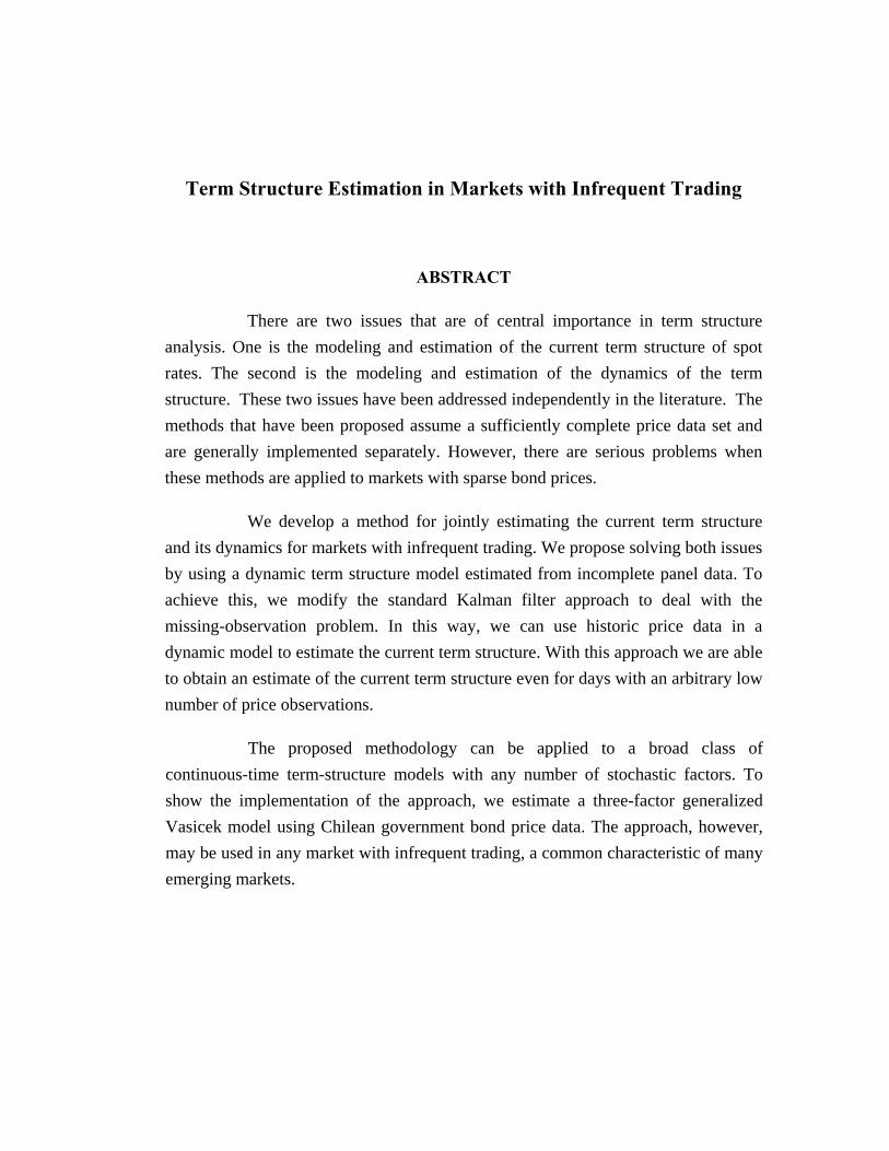
Figure 4 illustrates the sparseness or infrequent trading of daily bond transactions in Chile by showing for each day during the second semester of 2001 when a bond was traded or not. The panel-data shown is clearly incomplete, a condition that is critical in the choice of the estimation methodology.19
19 Curiously, the figure resembles a DNA pattern.

20
Table 1. Description of the data: Daily transactions of Chilean government inflation-protected pure discount and coupon bonds from January 1997 to December 2001.
Maturity Range(Years)
Number ofObservations
Average Trading
Frequency*
AverageYield**
Yield StandardDeviation**
0 - 1 1115 89.70% 5.81% 2.04%
1 - 1.5 377 30.33% 6.46% 1.83%1.5 - 2.5 426 34.27% 6.29% 1.45%2.5 - 3.5 443 35.64% 6.20% 1.17%3.5 - 4.5 642 51.65% 6.15% 1.17%4.5 - 5.5 519 41.75% 6.36% 1.12%5.5 - 6.5 550 44.25% 6.36% 0.87%6.5 - 7.5 766 61.63% 6.33% 0.91%7.5 - 8.5 921 74.09% 6.22% 0.81%8.5 - 9.5 451 36.28% 6.31% 0.80%
9.5 - 10.5 584 46.98% 6.31% 0.65%10.5 - 11.5 268 21.56% 6.30% 0.72%11.5 - 12.5 458 36.85% 6.21% 0.67%12.5 - 13.5 262 21.08% 6.20% 0.64%13.5 - 14.5 507 40.79% 6.14% 0.60%14.5 - 15.5 269 21.64% 6.10% 0.71%15.5 - 16.5 311 25.02% 6.13% 0.61%16.5 - 17.5 269 21.64% 6.18% 0.60%17.5 - 18.5 309 24.86% 6.32% 0.53%18.5 - 19.5 404 32.50% 6.32% 0.53%19.5 - 20 533 42.88% 6.26% 0.60%
Total 10384
**Continuous Compounding
Pure Discount Bonds
Coupon Bonds
*Trading frequency is defined as the number of days for which there is atransaction of a given bond over all available trading days.
21
0 1 2 3 4 5 6 7 8 9 10 11 12 13 14 15 16 17 18 19 200.03224256 0.05012399 0.050122610.03314705 0.0463109 0.0463109 0.04955178 0.05019394 0.05145328 0.0550562 0.0550562 0.05524547 0.055282270.03267019 0.04993237 0.04997993 0.05083569 0.05310465 0.05467756 0.05477224 0.05451975 0.05515085 0.055150850.02740139 0.04478214 0.04439959 0.04654956 0.04859967 0.0491635 0.05145328 0.05174215 0.05259245 0.05368294 0.05363555 0.05430738 0.053983010.03219057 0.04814234 0.04838192 0.04926624 0.05107327 0.05093073 0.05195974 0.05207445 0.05268732 0.05337092 0.053456510.03286377 0.04592893 0.04891714 0.04896533 0.05088321 0.05164323 0.05274424 0.05306672 0.053493370.03256219 0.04305949 0.04174956 0.04821857 0.05002749 0.05000768 0.0517382 0.05176193 0.05306672 0.05292446 0.05382509 0.05429877 0.054488180.03495657 0.05012411 0.05249757 0.05306672 0.05312994 0.05354077 0.05418432 0.05485056 0.055434710.03378013 0.04538756 0.04592893 0.050017040.03383304 0.05026527 0.05025998 0.05107327 0.05444084 0.054488180.03454163 0.04315527 0.04964694 0.049751390.03440825 0.0459926 0.04945661 0.04990587 0.05088321 0.05158444 0.05230778 0.05290414 0.05304775 0.05467756 0.054488180.0356514 0.04683588 0.04736057 0.05021772 0.05018602 0.05363555 0.054677560.0334695 0.04305949 0.04497336 0.04554681 0.04592893 0.04917104 0.04993638 0.05211795 0.05429877 0.05401459 0.05463022 0.05465389
0.03479536 0.04978966 0.04978015 0.05358816 0.05448818 0.05448818 0.054677560.03439727 0.05021486 0.0512633 0.05308252 0.05373032 0.0538014 0.05453553 0.05453553 0.05477224 0.054393490.03518736 0.046979 0.050217720.03507643 0.04497336 0.04583342 0.0475513 0.04736057 0.05021772 0.05172633 0.0553401 0.05526913 0.05543471 0.05534010.05165274 0.05306672 0.05515085 0.05515085 0.054961560.05693881 0.04831386 0.0504079 0.05064558 0.05401459 0.05420406 0.05571849 0.055488760.05477315 0.04955178 0.05095924 0.05548201 0.05586035 0.056002190.05675661 0.05354077 0.04688359 0.05182049 0.05171446 0.056474850.06059129 0.0480518 0.04997993 0.05145328 0.05173819 0.05396722 0.05496156 0.05567908 0.05559369 0.0553401 0.055340090.06929286 0.046979 0.0475513 0.04760579 0.04869492 0.05097824 0.05107327 0.05325636 0.05422774 0.05420406 0.05481957 0.05496156 0.054961560.06854219 0.04592893 0.04585464 0.04736057 0.04783733 0.05107327 0.05145328 0.05325636 0.05429877 0.05439349 0.05583671 0.05562390.06963685 0.04583342 0.04545126 0.04592893 0.05325636 0.05619128 0.056191280.05828173 0.04545126 0.04592893 0.04688359 0.051643230.06665192 0.04807562 0.05145328 0.05145328 0.05590763 0.05638034 0.05638034 0.05638034
0.04926624 0.05156093 0.05448818 0.056758340.06253141 0.04629181 0.04805974 0.05164323 0.057230630.0701727 0.04678816 0.04688359 0.04783733 0.05335118 0.05467756 0.05539529 0.05805662
0.06496817 0.04859967 0.04891714 0.05164323 0.05373032 0.05429877 0.05543471 0.05543471 0.0586462 0.05910582 0.05878764 0.05874049 0.058268910.0569815 0.05078817 0.05311413 0.05320896 0.05526322 0.05534956 0.05760831 0.05902334 0.05890886 0.05883479
0.06401926 0.046979 0.0475513 0.05344597 0.05410933 0.05656935 0.05647485 0.05915295 0.059023340.05858555 0.04955178 0.05344597 0.05798585 0.05958879 0.05977720.06168579 0.04974209 0.04736057 0.05439349 0.05444084 0.05515085 0.058929070.0503442 0.04914724 0.05420406 0.05420406 0.05537163 0.0566166 0.05817456 0.05845757
0.04783733 0.05429877 0.05496426 0.05699451 0.05823746 0.058245320.05354077 0.05543471 0.05836325 0.05817456
0.04821857 0.04845677 0.05306672 0.05293124 0.05543471 0.05534009 0.056663850.04350927 0.04592893 0.04736057 0.04736057 0.05102576 0.0512633 0.05172764 0.05240268 0.05410933 0.0548669 0.05496156 0.05600219 0.057041740.0409509 0.04401689 0.04688359 0.04945661 0.04974209 0.05026527 0.05106535 0.05128467 0.05344597 0.0551193 0.05552931
0.03437574 0.04688359 0.05112078 0.05135829 0.05179517 0.0553401 0.055718490.02982381 0.04611993 0.0510416 0.05183315 0.05216818 0.05259245 0.0564951 0.05656935 0.05656935 0.056569350.03334086 0.04545126 0.05207049 0.05205467 0.05249757 0.05638033 0.0570260.00548295 0.0415857 0.05164323 0.05249283 0.05425142 0.05638034 0.05713619 0.05713619
-0.01501203 0.05248319 0.05590763 0.05628581 0.05621019 0.05685281 0.05675834-0.02102432 0.02858746 0.04152574 0.04305949 0.04425609 0.04524739 0.05237658 0.05645122 0.05638034 0.05671109-0.01421161 0.057230630.00351594 0.04401689 0.04551496 0.05195974 0.05675834
-0.02389384 0.0428679 0.04569013 0.0488854 0.05128623 0.05249757 0.05543471 0.05609674 0.05604454 0.05586035 0.05606522-0.0261132 0.04401689 0.04580953 0.05135829 0.05168988 0.05581306 0.05581306 0.05623855 0.05628581 0.056214910.03685438 0.03913658 0.05122107 0.05182366 0.0553401
-0.02071134 0.0390925 0.05077366 0.05123954 0.05382509 0.05448818 0.0553401 0.0549584 0.05499753-0.01824861 0.02849027 0.03854741 0.03922071 0.04046993 0.04993237 0.04992345 0.05401459 0.05396722 0.05453553 0.05456935
0.03700673 0.03915661 0.04938622 0.05069311 0.05396722 0.05420406 0.054288250.03405773 0.04774199 0.04856395 0.0494445 0.05002749 0.05249757 0.05259245 0.05458288 0.0547249 0.054440840.0324666 0.04545126 0.04858776 0.04899845 0.05019394 0.04993237 0.05259245 0.05410933 0.05415669 0.05401459 0.05382509
0.03420817 0.03527061 0.0394803 0.04130188 0.048393 0.05116829 0.05297189 0.05401459 0.05382509 0.053540770.03156205 0.03912455 0.04834562 0.05306672 0.05346967 0.05388826 0.053919840.03244159 0.04793265 0.05021772 0.05211795 0.05306672 0.05292446 0.05316155 0.05335118 0.05354077 0.05354077
0.03419437 0.03917264 0.04545126 0.0479962 0.04802797 0.04964694 0.05059805 0.05228066 0.05287704 0.053208960.03200525 0.03507753 0.03792179 0.04497336 0.04277209 0.04435176 0.04821857 0.05211795 0.05365924 0.05382509 0.05420406
0.04449524 0.04879016 0.05316155 0.053161550.02664193 0.03355566 0.03944505 0.03912455 0.04736057 0.05287704 0.052877040.03436922 0.03681397 0.03970137 0.04042191 0.04564236 0.04736057 0.04936143 0.04974209 0.05448818 0.05477224
0.04764665 0.04879016 0.04917104 0.04974209 0.054393490.04396904 0.04807562 0.04833292 0.05230778 0.05240268 0.05287704 0.0527229
0.03893221 0.04106996 0.04162167 0.04808992 0.04821857 0.05230778 0.05259245 0.05259245 0.053066720.03349115 0.04740826 0.04859967 0.05211795
0.03902839 0.04104597 0.05159575 0.05207049 0.05226033 0.052307780.03541804 0.03825871 0.04018179 0.04114194 0.04974209 0.05164323 0.05145328 0.05183315 0.051500770.03541974 0.03575317 0.03902839 0.04487776 0.04688359 0.05202303 0.05183315 0.052402680.03636592 0.04015777 0.04018179 0.05240268 0.05230778
0.04640637 0.04707441 0.04731288 0.05107327 0.05135829 0.05211795 0.05221287 0.052402680.04659729 0.04659729 0.04688359 0.05192809 0.05183315 0.05183315 0.052117950.04583342 0.04687166 0.05164323 0.05169072 0.0518859
0.04726519 0.04726519 0.05221287 0.052133770.0429637 0.03922071 0.04699808 0.04783733
0.03797516 0.04688359 0.046979 0.05059805 0.05211795 0.052212870.03690133 0.03825871 0.04123791 0.04688359 0.0504079 0.05088321 0.051453280.03625274 0.03832287 0.03888412 0.04114194 0.03912455 0.0459926 0.0504079 0.05202303 0.05188062 0.05202303 0.05211795
0.04027785 0.04487776 0.05059805 0.052023030.03726029 0.03869173 0.03825871 0.0463109 0.04688359 0.05135829 0.05164323 0.051643230.0368868 0.04210118 0.04152574 0.03931686 0.04018179 0.04497336 0.04991334 0.05088321 0.05097824 0.05132663 0.05173819
0.03833414 0.04037389 0.04037389 0.04397435 0.04592893 0.04640637 0.04745594 0.05050298 0.05154826 0.05078817 0.05126330.03962759 0.04611993 0.050645580.04025162 0.03517407 0.04147778 0.04611993 0.05097824 0.05088321 0.05145328
0.045928930.04128963 0.04569013 0.04640637 0.0482821 0.050693110.0436218 0.04123791 0.04545126 0.04592893 0.04773246 0.05040790.0423335 0.04392118 0.04305949 0.04640637 0.04983724 0.04983724 0.0504396 0.05083569 0.05097824 0.05097824
0.04344256 0.04315527 0.04497336 0.04645411 0.04831386 0.05021772 0.05097824 0.051239540.04392119 0.04358617 0.04372976 0.04596077 0.04650184 0.04831386 0.050027490.04678816 0.04745594 0.04793265 0.04783733 0.04974209
0.04347447 0.04439959 0.04545126 0.04774199 0.05116829 0.0512633 0.052117950.04765619 0.05240268
0.04764665 0.047932650.04593661 0.04850441 0.04859967 0.05225013 0.05164323
0.04745594 0.053540770.04583342 0.04778966 0.04821857 0.04917104 0.04917104 0.05344597
0.04821857 0.04926624 0.04944736 0.04952799 0.05188379 0.05228774 0.053445970.04736057 0.05069311
0.04650183 0.04936143 0.04936143 0.05202303 0.05287704 0.053066720.04526013 0.04850441 0.052307780.04525249 0.04669273 0.04707441 0.04774199 0.05202303 0.05164323 0.05211795 0.05221287 0.05233941
0.04472477 0.04500922 0.046979 0.04812327 0.048123270.0435383 0.04409939 0.04478214 0.04812327 0.04831386 0.05202303 0.05234574
0.04564236 0.04452393 0.044734330.0435383 0.04592893 0.0471698 0.05021772 0.05173819 0.05202303 0.05211795 0.05205467
0.0439722 0.04305949 0.0433468 0.04526013 0.04533295 0.04669273 0.04654956 0.04793265 0.05050298 0.05116829 0.05159575 0.05155776 0.051928090.03762985 0.04305949 0.04385738 0.04468652 0.04573789 0.04683588 0.04669273 0.05200721 0.051928090.04072528 0.04200529 0.0436819 0.04358617 0.04688359 0.04688359 0.05154826 0.05161949 0.05197556
0.04392118 0.04449524 0.04564236 0.04659729 0.04664501 0.05112078 0.051358290.0418135 0.04347447 0.0433468 0.04650184 0.05069311 0.05097824 0.05097824
0.04248461 0.04602444 0.04614381 0.05002749 0.05070896 0.050835690.04219705 0.0435383 0.04635864 0.04669273 0.05078817
0.0429637 0.04666887 0.05116829 0.05107327 0.051073270.03936837 0.04162167 0.04305949 0.0463109 0.05050298 0.05085945 0.050978240.04379884 0.04066198 0.049551780.04194804 0.04114194
Bond Maturity (Years)
Chr
onol
ogic
al T
ime
Jul. 2001
Dec. 2001
Fig. 4. Graphical description of available Chilean government inflation-protected discount and coupon bond daily data for the second semester of 2001. A black cell
indicates that data was available for the corresponding maturity at a given day.
5.2 Estimation results
We estimate the 3-factor Vasicek model parameters using bond price transactions data from January 1997 to December 2001. As noted in section 4, the Kalman filter considers measurement errors in the observations. For simplicity we

22
assume that the error variance-covariance matrix tR is diagonal. Also, we aggregate
bonds into 5 groups depending on their maturities: the first group includes the discount bonds with maturities up to 1 year, and the next 4 groups include coupon bonds with maturities ranging from 1 to 5 years, from 6 to 10 years, from 11 to 15 years and from 16 to 20 years, respectively. Bonds within each group are assumed to have measurement errors with the same standard deviation: dξ , 1
cξ , 2cξ , 3
cξ and 4cξ ,
respectively. With these assumptions 18 different parameters must be estimated20. Table 2 presents parameter estimates and their respective estimation errors. Note that all the parameters are statistically significant, though the mean reversion coefficient of the first factor is very small suggesting that this factor follows a process which is close to a random walk.
Note that the correlation between the factors is very high which may lead us to believe that two factors could be sufficient to explain the dynamics of the yield curve. However, we find that with 1 and 2 factors the total in-sample RMSE is 0.52% and 0.35% respectively, compared with 0.12% obtained using 3 factors. Therefore, this important difference in estimation errors suggests that a 3 factor model is necessary to explain the complex dynamics of the Chilean yield curve. See appendix C for estimation results using 1 and 2 factor Vasicek models.
20 Implementation issues of the model can be found in Appendix B.

23
Table 2. Parameter estimates and standard errors from daily transactions of Chilean government inflation-protected pure discount and coupon bonds from January 1997 to
December 2001.
1κ 0.00050 0.00012
2κ 1.11455 0.01681
3κ 2.16431 0.05362
1σ 0.01747 0.00019
2σ 0.29298 0.00466
3σ 0.32780 0.00647
21ρ - 0.91042 0.01258
31ρ 0.84189 0.02376
32ρ - 0.97121 0.00246
1λ - 0.00056 0.00002
2λ 0.01599 0.00418
3λ - 0.05213 0.01836
δ 0.05614 0.02654
dξ 0.00225 0.00014
1cξ 0.00225 0.00004
2cξ 0.00079 0.00001
3cξ 0.00027 0.00001
4cξ 0.00038 0.00001

24
To illustrate the ability of the approach to fit observed prices on a day with a large number of transactions, Figure 5 shows the yield curve derived from the model for 01/09/1997. We see that the model is able to fit very well observed yields and this is representative of the sample period.
Recall that in Figure 2 we illustrated the inability of the curve-fitting methods to provide for reliable long term rates for a day when only short term bonds where traded. Figure 6 shows the yield curve obtained for the same day (10/06/1999) using our proposed methodology. We see that the estimated yield curve not only correctly fits observed yields for that day, but also is consistent with the previous day observations. Note that the yield curve shown has been constructed using only prices for that particular day, and the dynamics of the interest rate process. We have not included the previous day curve in Figure 6 because it is almost identical to the curve shown. The model’s long-term yields for the current day, for which there is no data, are very close to the observed previous day long-term yields. Comparing Figure 6 with Figure 2 which correspond to the same date, this example illustrates that our approach provides much more stable curves than those obtained by curve fitting methods.
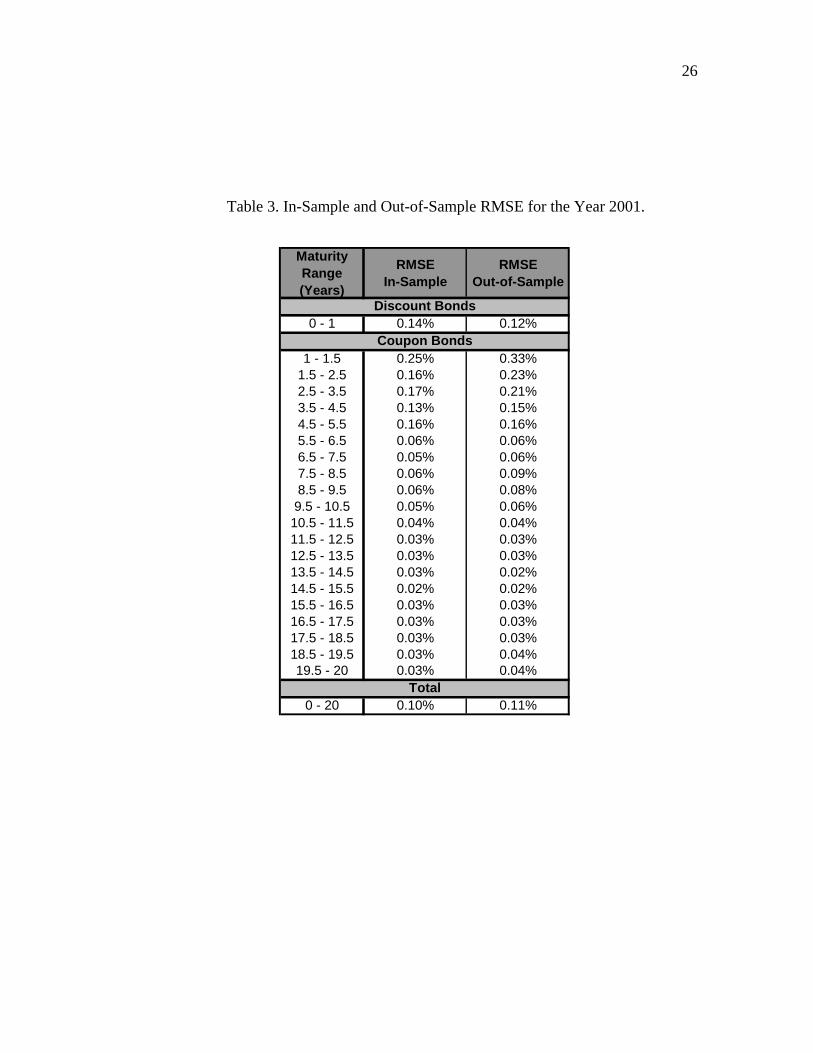
Table 3 presents in-sample and out-of-sample error measures by maturity. Out-of-sample error measures were calculated by re-estimating the model using data from 1997-2000, and then comparing yield curves obtained from the model to observed yields for the year 2001, which was not used in the parameter estimation. It can be seen that all errors are reasonably low, while errors for short term bonds are larger than for long term bonds. Out-of-sample errors are similar to in-sample errors, showing the stability of the model and its ability to be used in real world applications.

25
Bond Yields on
0%
2%
4%
6%
8%
0 5 10 15 20Maturity (Years)
Yiel
d (%
)
Observed Bond Yields
Model Term Structure
01/09/1997
Fig. 5. Estimated and observed coupon bond yields on 01/09/1997.
Bond Yields on
0%
2%
4%
6%
8%
0 5 10 15 20Maturity (Years)
Yiel
d (%
)
Previous Day Observed Bond YieldsObserved Bond YieldsModel Term Structure
10/06/1999
Fig. 6. Estimated and observed coupon bond yields on 10/06/1999.
26
Table 3. In-Sample and Out-of-Sample RMSE for the Year 2001.
Maturity Range(Years)
RMSEIn-Sample
RMSEOut-of-Sample
0 - 1 0.14% 0.12%
1 - 1.5 0.25% 0.33%1.5 - 2.5 0.16% 0.23%2.5 - 3.5 0.17% 0.21%3.5 - 4.5 0.13% 0.15%4.5 - 5.5 0.16% 0.16%5.5 - 6.5 0.06% 0.06%6.5 - 7.5 0.05% 0.06%7.5 - 8.5 0.06% 0.09%8.5 - 9.5 0.06% 0.08%9.5 - 10.5 0.05% 0.06%10.5 - 11.5 0.04% 0.04%11.5 - 12.5 0.03% 0.03%12.5 - 13.5 0.03% 0.03%13.5 - 14.5 0.03% 0.02%14.5 - 15.5 0.02% 0.02%15.5 - 16.5 0.03% 0.03%16.5 - 17.5 0.03% 0.03%17.5 - 18.5 0.03% 0.03%18.5 - 19.5 0.03% 0.04%19.5 - 20 0.03% 0.04%
0 - 20 0.10% 0.11%
Coupon Bonds
Total
Discount Bonds

27
Finally, we analyze the volatility term structure of spot interest rates and compare it to volatilities obtained directly from bond yields. The theoretical volatility structure of interest rates, which is independent of the state variables, is obtained by applying Ito’s lemma to Equation (8).
1/ 2
1 1
( ) ( ) ( )N N
R i j i j iji j
u uσ τ τ τ σ σ ρ= =
⎛ ⎞= ⎜ ⎟⎝ ⎠∑∑ (29)
where
1 exp( )( ) ii
i
kuk
ττ − −= − (30)
There are two difficulties in computing empirical estimates of the interest rate volatilities. First, most of the data consists of amortizing coupon bonds and we are interested in the volatility of spot rates. Second, the panel data contains many missing observations. To address these problems we aggregate the data in groups according to their maturity. The first group contains bonds with one to two years of maturity, and so on. Then, for each date we take the average yield of all the bonds in a given group and we compute the volatility of daily changes of these yields. In addition, we compute the average duration of the bonds in each group. To compare this empirical volatility to model spot volatilities, we assume that the volatility of each group represents the volatility of a discount bond with maturity equal to the average duration in the group.
Figure 7 shows the term structure of spot volatilities from the model and from the empirical estimates. Comparing this figure with Figure 3, we observe that our model volatilities are much closer to the empirical volatilities than those obtained using the curve fitting methods.

28
Fig. 7. Volatility Structure of Interest Rates 1997-2001.
6. Conclusion
The estimation of the term structure of interest rates is a critical issue, not only from a theoretical point of view, but also for all market participants including banks, regulators and financial institutions. It is an essential ingredient in the valuation and hedging of all fixed income securities. It is also necessary for financial planning and for implementing monetary policy. In economies with well developed and liquid financial markets, the existence of bond prices for a wide range of different maturities makes it easy to extract a term structure of spot rates that explains observed prices. Moreover, in some countries, such as the United States, zero-coupon bonds (Strips) of different maturities are individually traded. In many emerging markets, however, bonds trade infrequently so that for every particular day there are bond prices for only a few maturities. This missing-observation problem makes it difficult, and sometimes impossible, to estimate the term structure using only current data.
In this article we develop a methodology for using an incomplete panel-data of bond price observations to estimate the current term structure. We use an extended Kalman filter approach to estimate a dynamic multi-factor model of interest rates using the panel-data with missing observations. The Kalman filter estimation provides not only the parameters of the model but also the time series of the factors.
Volatility Structure of Interest Rates (1997-2001)
0%
2%
4%
6%
1,5 3,5 5,5 7,5 9,5 11,5 13,5
Maturity (Years)
Vola
tility
Model Volatility
Empirical Volatility from Bond Yields

29
The approach jointly estimates the current term structure and its dynamics. The model can be used to value and hedge all types of interest rate derivatives, including bonds with embedded options. This methodology also allows us to estimate the term structure for days with an arbitrary small number of traded bonds.
We implement the approach using a three-factor generalized Vasicek (1977) model and Chilean government bond data. The methodology, however, can be implemented with a broad class of dynamic interest rate models and in any market with infrequent trading, a very common situation in many emerging markets.
Our approach is currently being used by a consortium of financial and academic institutions in Chile to estimate the Chilean term structure of interest rates. The results are updated daily at the website RiskAmerica.com.

30
REFERENCES
ANDERSEN, T.G. and J. LUND (1997) Estimating continuous time stochastic volatility models of the short term interest rate. Journal of Econometrics, Vol. 77, 343-377.
BABBS, S.H. and K.B. NOWMAN (1999) Kalman filtering of generalized Vasicek term structure models. Journal of Financial and Quantitative Analysis, Vol. 34, N° 1, 115-130.
BALL, C. and W. TOROUS (1996) Unit roots and the estimation of interest rate dynamics. Journal of Empirical Finance, Vol. 3, 215-238.
BLISS, R.R. (1996) Testing term structure estimation methods. Advances in Futures and Operations Research, Vol. 9, 197-231.
BRENNAN, M.J., and E.S. SCHWARTZ (1979) A Continuous time approach to the pricing of bonds. Journal of Banking and Finance, Vol. 3, N° 2, 133-155.
BRENNER, R.J., R.H. HARJES, and K.F. KRONER (1996) Another look at models of the short-term interest rate. Journal of Financial and Quantitative Analysis, Vol. 31, 85-107.
BROZE, L., O. SCAILLET and J.-M. ZAKOIAN (1995) Testing continuous time models of the short-term interest rate. Journal of Empirical Finance, Vol. 2, 199-223.
CHAN, K.C., G.A. KAROLYI, F.A. LONGSTAFF and A.B. SANDERS (1992) Comparison models of the short-term interest rate. Journal of Finance, Vol. 47, 1209-1227.
CHEN, R.-R. and L. SCOTT (1993) Maximum likelihood estimation for a multifactor equilibrium model of the term structure of interest rates. Journal of Fixed Income, Vol. 3, 14-31.
CHEN, R.-R. and L. SCOTT (2003) Multi-factor Cox-Ingersoll-Ross models of the term structure: Estimates and tests from a Kalman filter model. Journal of Real Estate Finance and Economics, Vol. 27, N° 2.

31
CORTAZAR, G. and SCHWARTZ, E.S. (2003) Implementing a Stochastic Model for Oil Futures Prices. Energy Economics Vol. 25, N°3, 215-238.
COX, J.C., J. INGERSOLL, and S. ROSS (1985) A theory of the term structure of interest rates. Econometrica, Vol. 53, 385-407.
DAI, Q. and K.J. SINGLETON (2000) Specification analysis of affine term structure models. Journal of Finance, Vol. 55, N° 5, 1943-1978.
DE JONG, F. (2000) Time-series and cross-section information in affine term structure models. Journal of Business & Economics Statistics, Vol. 18, N° 3, 300-314.
DE JONG, F. and P. SANTA-CLARA (1999) The dynamics of the forward interest rate curve: A formulation with state variables. Journal of Financial and Quantitative Analysis, Vol. 34, N° 1, 131-157.
DEWACHTER, H. and K. MAES (2001) An admissible affine model for joint term structure dynamics of interest rates, Working Paper, Katholieke Universiteit Leuven.
DUAN, J.-C. and J.-G. SIMONATO (1995) Estimating and testing exponential-affine term structure models by Kalman filter, Working Paper, CIRANO.
DUFFIE, D. and R. KAN (1996) A yield-factor model of interest rates. Mathematical Finance, Vol. 6, 379-406.
DUFFIE, D. and K.J. SINGLETON (1997) An econometric model of the term structure of interest-rate swap yields. Journal of Finance, Vol. 52, N° 4, 1287-1321.
FISHER, M., D. NYCHKA, and D. ZERVOS (1994) Fitting the term structure of interest rates with smoothing splines, Working Paper, Federal Reserve Board of Governors.
GEYER, A.L.J. and S. PICHLER (1999) A state-space approach to estimate and test multifactor Cox-Ingersoll-Ross models of the term structure, Journal of Financial Research, Vol. 22, N° 1.
HAMILTON, J.D. (1994) Time series analysis, Princeton University Press, Princeton, N.J.

32
HARVEY, A.C. (1989) Forecasting, structural time series models and the Kalman filter, Cambridge University Press, Cambridge.
HEATH, D., R. JARROW, and A. MORTON (1992) Bond pricing and the term structure of interest rates: A new methodology for contingent claims valuation. Econometrica, Vol. 60, 77-105.
HO, T.S.Y. and S. LEE (1986) Term structure movements and the pricing of interest-rate contingent claims. Journal of Finance, Vol. 51, N° 5, 1011-1029.
LANGETIEG, T.C. (1980) A multivariate model of the term structure. Journal of Finance, Vol. 35, N° 1, 71-97.
LUND, J. (1994) Econometric analysis of continuous-time arbitrage-free models of the term structure of interest rates, Working Paper, The Aarhus School of Business.
LUND, J. (1997) Non-linear Kalman filtering techniques for term-structure models, Working Paper, The Aarhus School of Business.
MCCULOCH, J.H. (1971) Measuring the term structure of interest rates. Journal of Business, Vol. 44, N° 1, 19-31.
MCCULOCH, J.H. (1975) The tax adjusted yield curve. Journal of Finance, Vol. 30, N° 3, 811-830.
NELSON, C.R. and A.F. SIEGEL (1987) Parsimonious modeling of yield curves. Journal of Business, Vol. 60, N° 4, 473-489.
NOWMAN, K.B. (1997) Gaussian estimation of single-factor continuous time models of the term structure of interest rates. Journal of Finance, Vol. 52, 1695-1706.
NOWMAN, K.B. (1998) Continuous time short rate interest rate models. Applied Financial Economics, Vol. 8, 401-407.
ØKSENDAL, B. (1998) Stochastic differential equations : an introduction with applications. 5th ed., Springer, Berlin ; New York.

33
PEARSON, N.D. and T.-S. SUN (1994) Exploiting the conditional density in estimating the term structure: An application to the Cox, Ingersoll, and Ross model. Journal of Finance, Vol. 49, N° 4, 1279-1304.
PENNACCHI, G.G. (1991) Identifying the dynamics of real interest rates and inflation: Evidence using survey data. Review of Financial Studies, Vol. 4, N° 1, 53-86.
SCHWARTZ, E.S. (1997) The stochastic behavior of commodity prices: Implications for valuation and hedging. Journal of Finance, Vol. 52, N° 3, 923-973.
SCHWARTZ, E.S. and J.E. SMITH (2000) Short-term variations and long-term dynamics in commodity prices. Management Science, Vol. 46, 893-911.
SØRENSEN, C. (2002) Modeling seasonality in agricultural commodity futures. Journal of Futures Markets, Vol. 22, 393-426.
SVENSSON, L.E.O. (1994) Estimating and interpreting forward interest rates: Sweeden 1992-1994, Working Paper, National Bureau of Economic Research.
VASICEK, O.A. (1977) An equilibrium characterization of the term structure. Journal of Financial Economics, Vol. 5, N° 2, 177-188.
VASICEK, O.A. and H.G. FONG (1982) Term structure modeling using exponential splines. Journal of Finance, Vol. 37, N° 2, 339-356.

34
APPENDIX A
The Nelson and Siegel (1987) approach assumes that the forward rate curve is of the following form:
1 10 1 2
1
( )T TTf T e eτ τβ β β
τ
− −
= + + (31)
where T is the time to maturity, and 0β , 1β , 2β and 1 0τ > are parameters.
The spot rates can then be calculated as the integral of forward rates:
0 1 20
1( ) ( ) (1 ) ((1 ) )T T T T
R T f s ds e e eT T T
τ τ ττ τβ β β− − −
= = + − + − −∫ (32)
Svensson (1994) proposes a generalization of Nelson and Siegel (1987) introducing a new term in the forward rate curve:
1 1 20 1 2 3
1 2
( )T T TT Tf T e e eτ τ τβ β β β
τ τ
− − −
= + + + (33)
where the new parameters are 3β and 2 0τ > .
In both cases, coupon bond prices are calculated discounting each coupon at the corresponding spot rate. The parameters of the models can then be estimated by minimizing the quadratic errors in bond prices or yields.
APPENDIX B
In this appendix we describe in detail how to apply the methodology developed in Section 4 to the generalized Vasicek model introduced in Section 3, with an incomplete panel-data set of discount and coupon bond yields.
The transition equation of the state variables under a generalized Vasicek model is independent of the observations, and the associated terms appearing in equation (12) are:

35
(1 )t n idiag k t= − ∆A 1
t
n
t
t
λ
λ
− ∆⎛ ⎞⎜ ⎟= ⎜ ⎟⎜ ⎟− ∆⎝ ⎠
c M (34)
21 1 1
21 1
n n
t
n n n
tσ σ σ ρ
σ σ ρ σ
⎛ ⎞⎜ ⎟
= ∆⎜ ⎟⎜ ⎟⎝ ⎠
QL
M O M
L
(35)
where ( )n idiag x stands for a diagonal n n× matrix whose ( , )i i element is ix , t∆ is
the time interval at which yields are observed, and other parameters are the ones appearing in equation (4).
Let dtm and c
tm be the number at time t of observed discount and
coupon bonds respectively and , 1
dtnd
i t iτ
= and , 1
ctnc
i t iτ
= the sets containing their
respective associated maturities. The vector of observations tz is then:
dt
t ct
⎛ ⎞= ⎜ ⎟⎝ ⎠
zz
z (36)
where dtz and c
tz are 1dtm × and 1c
tm × vectors containing the observed yields of discount and coupon bonds respectively. Of course, either d
tm or ctm can be zero, but
not both at the same time.
The parameters of the measurement equation are:
dt
t ct
⎛ ⎞= ⎜ ⎟⎝ ⎠
HH
H
dt
t ct
⎛ ⎞= ⎜ ⎟⎝ ⎠
dd
d (37)
where
1,
1,
,
,
( )
( )dt
dt
dt
dt
dt
dm tdm t
ττ
τ
τ
⎛ ⎞′⎜ ⎟−⎜ ⎟⎜ ⎟
= ⎜ ⎟⎜ ⎟′⎜ ⎟−⎜ ⎟⎜ ⎟⎝ ⎠
u
HuM
1,1
1 ,
ˆ( , )
ˆ( , )ct
ctt t
ct
ct t m t
y
y
τ
τ
−
−
∂⎛ ⎞⎜ ⎟′∂⎜ ⎟
= ⎜ ⎟⎜ ⎟∂⎜ ⎟⎜ ⎟′∂⎝ ⎠
xx
H
xx
M (38)

36
1,
,
( )
( )dt
dt
dt
dm t
v
v
τ
τ
⎛ ⎞−⎜ ⎟
= ⎜ ⎟⎜ ⎟−⎝ ⎠
d M
1, 1,1 1 1
1 1 1, ,
ˆ ˆ ˆ( , ) ( , )
ˆ ˆ ˆ( , ) ( , )c ct t
c ct tt t t t t t
ct
c ct t t t t tm t m t
y y
y y
τ τ
τ τ
− − −
− − −
⎛ ∂ ⎞⎛ ⎞− ⎜ ⎟⎜ ⎟′∂⎝ ⎠⎜ ⎟⎜ ⎟=⎜ ⎟
∂⎛ ⎞⎜ ⎟− ⎜ ⎟⎜ ⎟′∂⎝ ⎠⎝ ⎠
x x xx
d
x x xx
M (39)
The gradient of the yield with respect state variables can be computed by differentiating implicitly equation (10) with respect the state variables:
( ) ( )
( )
1 1
1
exp ( ) ( ) exp ( , )
( , )exp ( , )
M MT
j j jj j
M
jj
v y
yyy
τ τ τ τ
ττ τ
= =
=
⎛ ⎞ ⎛ ⎞∂ ∂+ = −⎜ ⎟ ⎜ ⎟∂ ∂⎝ ⎠ ⎝ ⎠
⎛ ⎞∂ ∂= −⎜ ⎟∂ ∂⎝ ⎠
∑ ∑
∑
u x xx x
xxx
(40)
so that:
( )
( )1
1
( ) exp ( ) ( )( , )
exp ( , )
MT
j j jj
M
j jj
vy
y
τ τ ττ
τ τ τ
=
=
+∂
=∂ − −
∑
∑
u u xxx x
(41)
The remaining parameters to be specified belong to the covariance matrix of measurement errors. In this paper, we assume that this covariance matrix is diagonal and can only have 5 different parameters: dξ , 1
cξ , 2cξ , 3
cξ and 4cξ . The first
of them corresponds to the variance of measurement errors of discount bonds. The remaining 4 parameters correspond to the variance of coupon bonds for maturities ranging between 1 to 5 years, 6 to 10 years, 11 to 15 years and 16 to 20 years respectively. Therefore, the covariance matrix of measurement errors is:
dt
t ct
⎛ ⎞= ⎜ ⎟⎝ ⎠
R 0R
0 R (42)
where ( )dt
d dt n
diag=R ξ and ( )ct
c ct jn
diag=R ξ .

37
APPENDIX C
In this appendix we report additional results of our estimation. Tables 4 and 5 show the parameter estimates using a 1 and a 2 factor model using the same data set (1997-2001). We find that for both models, most parameters are statistically significant. Also, as in the 3 factor model case, the 2 factor model shows a very small mean reversion coefficient for the first factor, suggesting that this factor might follow a process close to a random walk. This does not happen with the 1 factor model.
Table 6 shows in-sample RMSE estimation errors for 1, 2 and 3 factor models. We can see that the 1 factor model does not price satisfactorily discount and coupon bonds. The 2 factor model behaves similar to the 3 factor model for pricing coupon bonds, although it does not price accurately discount bonds, which accounts for more than 10% of all available transactions. That explains why the overall in-sample RMSE for the 2 factor model is much higher than for the 3 factor model.

38
Table 4. Parameter estimates and standard errors using a 1 factor Vasicek model from daily transactions of Chilean government inflation-protected pure discount and coupon
bonds from January 1997 to December 2001.
1κ 0.20616 0.00376
1σ 0.01545 0.00050
1λ -0.00365 0.00855
δ 0.04738 0.04147
dξ 0.01413 0.00030
1cξ 0.00483 0.00008
2cξ 0.00122 0.00002
3cξ 0.00034 0.00001
4cξ 0.00083 0.00002

39
Table 5. Parameter estimates and standard errors using a 2 factor Vasicek model from daily transactions of Chilean government inflation-protected pure discount and coupon
bonds from January 1997 to December 2001.
1κ 0.00052 0.00067
2κ 0.87364 0.01584
1σ 0.01299 0.00036
2σ 0.08172 0.00287
21ρ -0.86349 0.01141
1λ -0.00012 0.00005
2λ -0.00444 0.00481
δ 0.05039 0.05647
dξ 0.01031 0.00024
1cξ 0.00229 0.00005
2cξ 0.00090 0.00002
3cξ 0.00029 0.00001
4cξ 0.00039 0.00001

40
Table 6. In-Sample RMSE for 1997-2001 using 1, 2 and 3 factors Vasicek models.
3 Factors 2 Factors 1 Factor
0 - 1 0.11% 1.01% 1.41%
1 - 1.5 0.25% 0.25% 0.79%1.5 - 2.5 0.29% 0.29% 0.60%2.5 - 3.5 0.17% 0.17% 0.36%3.5 - 4.5 0.15% 0.16% 0.31%4.5 - 5.5 0.18% 0.18% 0.28%5.5 - 6.5 0.07% 0.08% 0.16%6.5 - 7.5 0.09% 0.10% 0.14%7.5 - 8.5 0.08% 0.10% 0.11%8.5 - 9.5 0.08% 0.09% 0.10%9.5 - 10.5 0.04% 0.05% 0.06%10.5 - 11.5 0.04% 0.05% 0.04%11.5 - 12.5 0.02% 0.02% 0.02%12.5 - 13.5 0.04% 0.04% 0.03%13.5 - 14.5 0.02% 0.02% 0.03%14.5 - 15.5 0.03% 0.03% 0.04%15.5 - 16.5 0.04% 0.04% 0.06%16.5 - 17.5 0.03% 0.04% 0.07%17.5 - 18.5 0.03% 0.03% 0.07%18.5 - 19.5 0.03% 0.03% 0.09%19.5 - 20 0.03% 0.03% 0.10%
0 - 20 0.12% 0.35% 0.52%
Maturity Range(Years)
RMSEIn-Sample
(1997-2001)
Discount Bonds
Coupon Bonds
Total
Recommended