Testing Multiple Hypotheses and
False Discovery RateModels, Inference, and Algorithms
Primer
Manuel A. Rivas Broad Institute
Let’s assume that we wish to examine the association between a response and
m different covariates

When m tests are performed, the aim is to decide which of the nulls should be rejected.

Not flagged Flagged
H0
H1
Not flagged Flagged
H0
H1
K
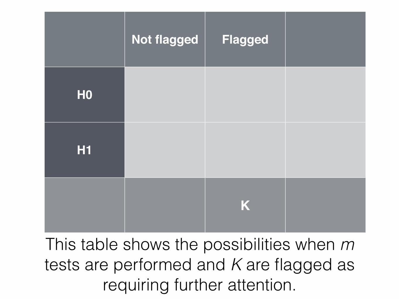
This table shows the possibilities when m tests are performed and K are flagged as
requiring further attention.

Not flagged Flagged
H0 m0
H1
K
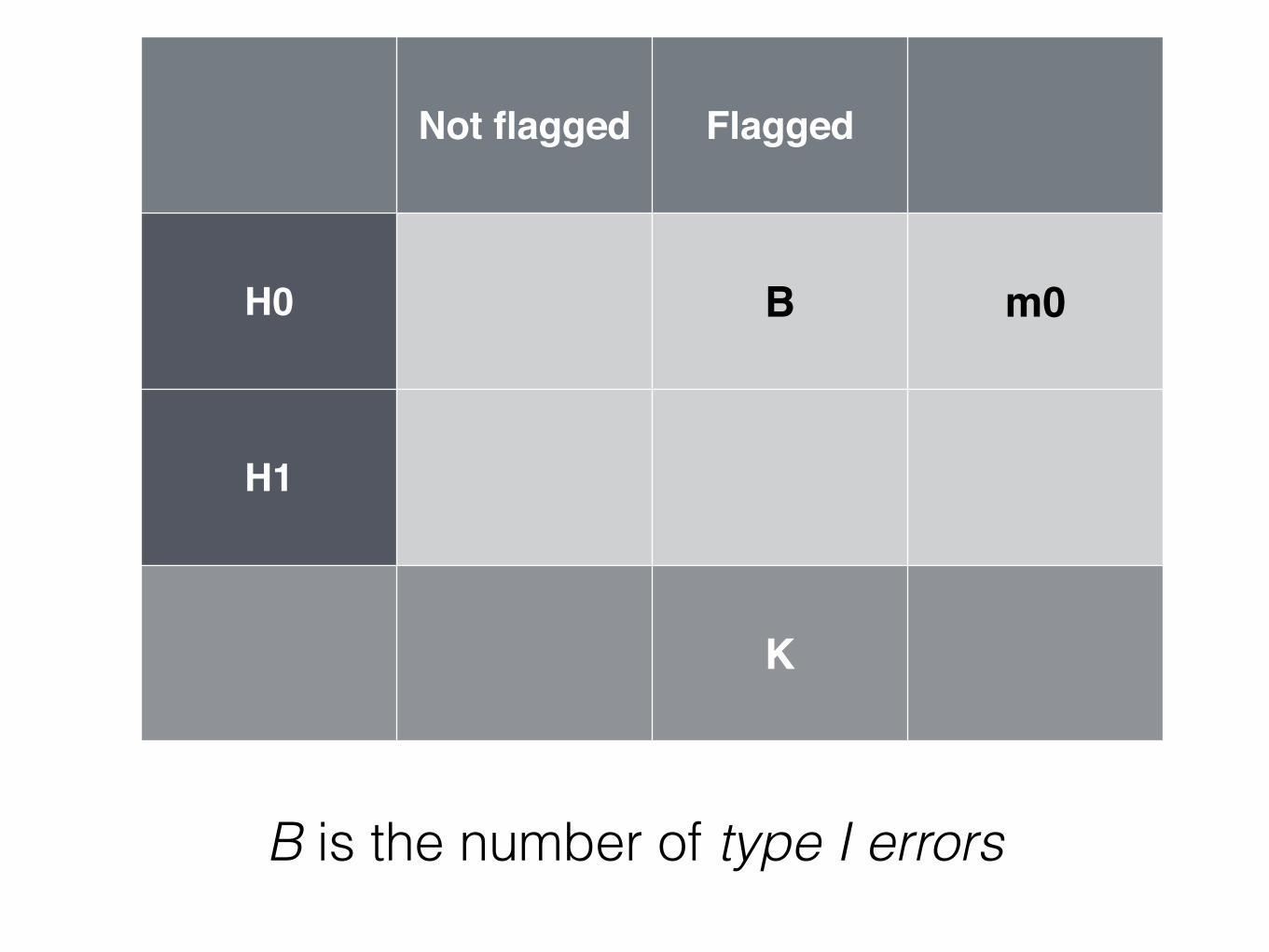
m0 is the number of true nulls
Not flagged Flagged
H0 B m0
H1
K
B is the number of type I errors

Not flagged Flagged
H0 B m0
H1 C
K
C is the number of type II errors

Not flagged Flagged
H0 A B m0
H1 C D m1
m - K K m
m1 is the number of true alternatives

Not flagged Flagged
H0 A B m0
H1 C D m1
m - K K m
Each of these quantities is unknown. The aim is to select a rule on the basis of some
criterion and this in turn will determine K.
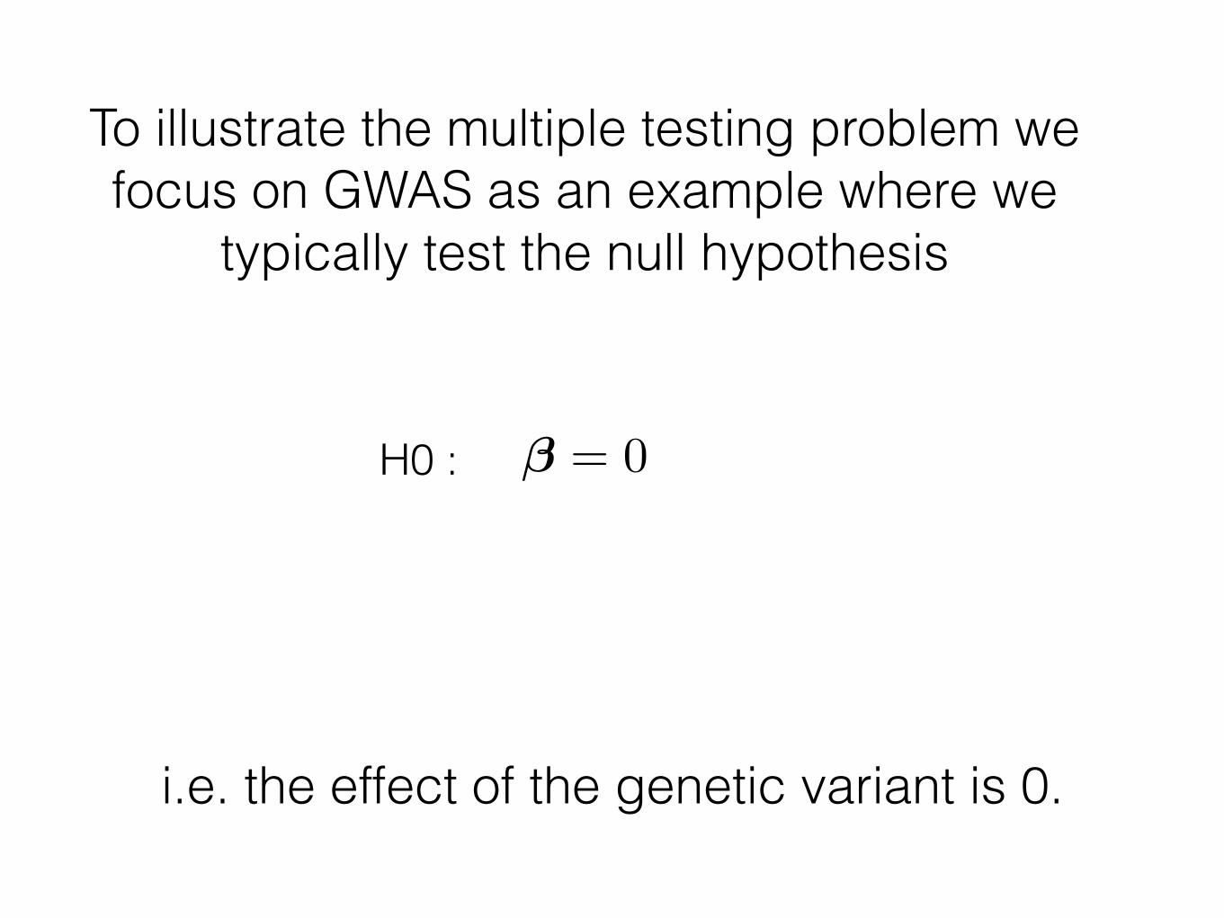
To illustrate the multiple testing problem we focus on GWAS as an example where we
typically test the null hypothesis
H0 : � = 0
i.e. the effect of the genetic variant is 0.
In a single test situation the historical emphasis has been on the control of the
type I error rate (false positives).
In a multiple testing situation there are a variety of criteria that may be considered.

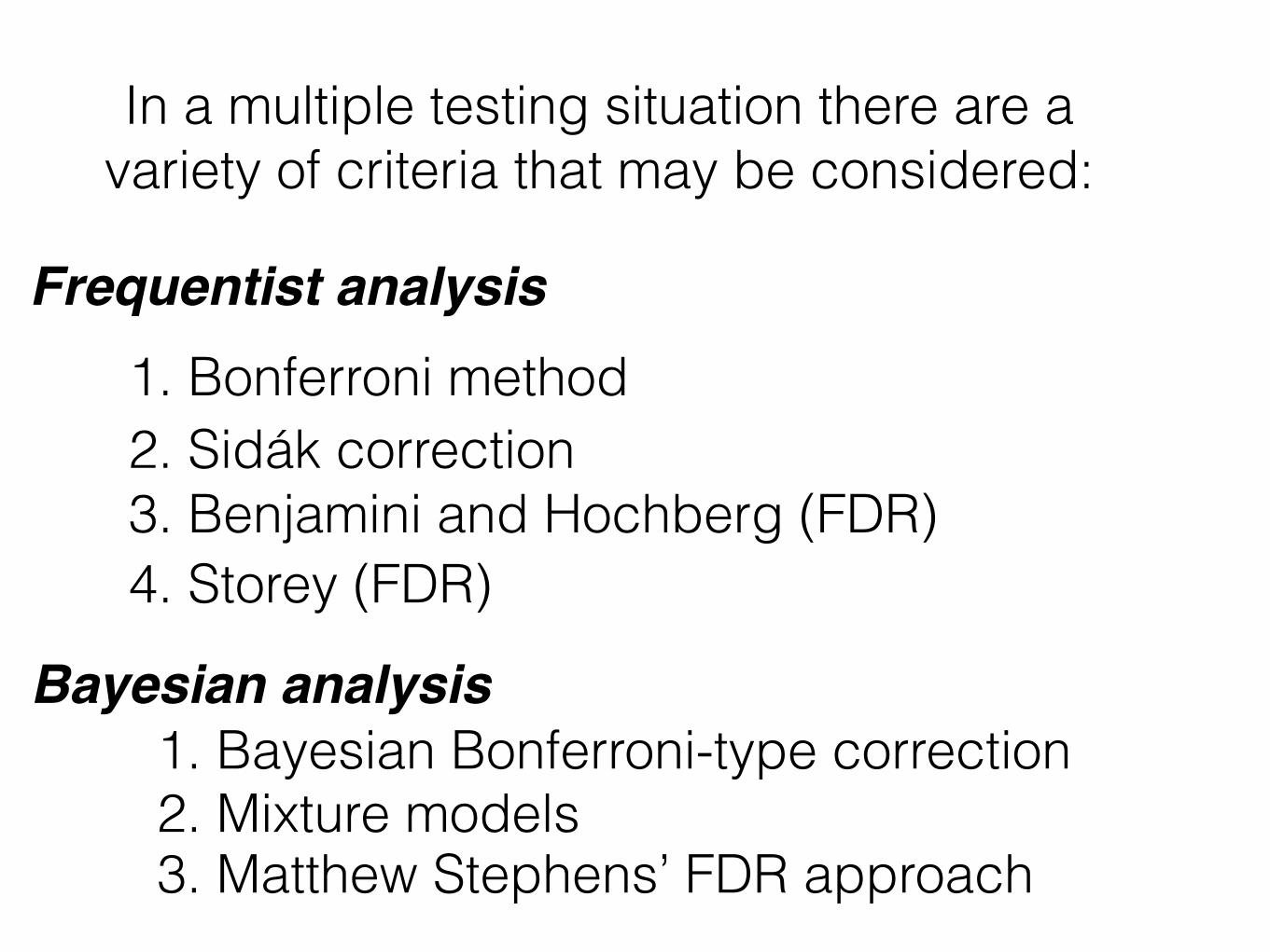
In a multiple testing situation there are a variety of criteria that may be considered:
1. Bonferroni method 2. Sidák correction 3. Benjamini and Hochberg (FDR) 4. Storey (FDR)
Frequentist analysis
In a multiple testing situation there are a variety of criteria that may be considered:
1. Bonferroni method 2. Sidák correction 3. Benjamini and Hochberg (FDR) 4. Storey (FDR)
Frequentist analysis
Bayesian analysis1. Bayesian Bonferroni-type correction 2. Mixture models 3. Matthew Stephens’ FDR approach

In a multiple testing situation there are a variety of criteria that may be considered:
1. Bonferroni method2. Sidák correction3. Benjamini and Hochberg (FDR) 4. Storey (FDR)
Frequentist analysis
Bayesian analysis 1. Bayesian Bonferroni-type correction 2. Mixture models 3. Matthew Stephens’ FDR approach

Family-wise error rate (FWER): the probability of making at least one type I error
Frequentist analysis

Family-wise error rate (FWER): the probability of making at least one type I error
Frequentist analysis
P (B � 1|H1 = 0, . . . , Hm = 0)
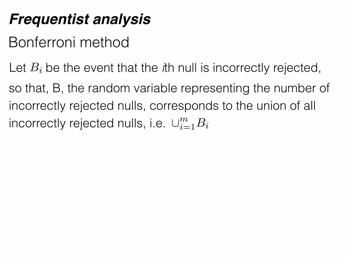
Bonferroni method Frequentist analysis
Let be the event that the ith null is incorrectly rejected,so that, B, the random variable representing the number of incorrectly rejected nulls, corresponds to the union of all incorrectly rejected nulls, i.e.
Bi
[mi=1Bi

Bonferroni method Frequentist analysis
With a common level for each test ↵⇤
the family-wise error rate (FWER) is
↵F = P (B � 1|H1 = 0, . . . , Hm = 0) = P ([mi=1Bi|H1 = 0, . . . , Hm = 0)
mX
i=1
P (Bi|H1 = 0, . . . , Hm = 0)
= m↵⇤

Bonferroni method Frequentist analysis
↵F = P (B � 1|H1 = 0, . . . , Hm = 0) = P ([mi=1Bi|H1 = 0, . . . , Hm = 0)
mX
i=1
P (Bi|H1 = 0, . . . , Hm = 0)
= m↵⇤
The Bonferroni method takes ↵⇤ = ↵F /m
to give FWER ↵F .

Bonferroni method Frequentist analysis
Preferred approach for GWAS where to control the FWER at a level of alpha = 0.05 with m = 1,000,000 tests, we would take
↵⇤ = .05/1, 000, 000 = 5⇥ 10�8.
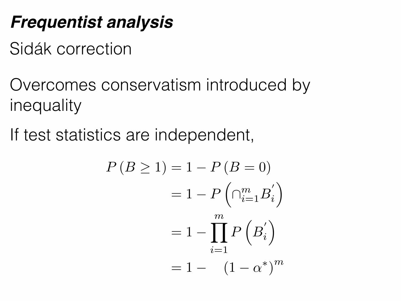
Sidák correction Frequentist analysis
Overcomes conservatism introduced by inequality If test statistics are independent,
P (B � 1) = 1� P (B = 0)
= 1� P⇣\mi=1B
0
i
⌘
= 1�mY
i=1
P⇣B
0
i
⌘
= 1� P (1� ↵⇤)m

Sidák correction Frequentist analysis
Overcomes conservatism introduced by inequality If test statistics are independent,
↵⇤ = 1� (1� ↵F )1/m .
In GWAS, assuming 1,000,000 tests were independent this would change it slightly to 5.13e-8 as a p-value threshold.

False Discovery Rate (FDR) Frequentist analysis
A simple way to overcome the conservative nature of the control of FWER is to increase ↵F .

False Discovery Rate (FDR) Frequentist analysis
A simple way to overcome the conservative nature of the control of FWER is to increase ↵F .
One measure to calibrate a procedure is via the expected number of false discoveries:
EFD = m0 ⇥ ↵⇤
m⇥ ↵⇤

False Discovery Rate (FDR) Frequentist analysis
A simple way to overcome the conservative nature of the control of FWER is to increase ↵F .
One measure to calibrate a procedure is via the expected number of false discoveries:
EFD = m0 ⇥ ↵⇤
m⇥ ↵⇤Recall m0 is the number of true nulls.

False Discovery Rate (FDR) Frequentist analysis
For example, we could specify ↵⇤ such that EFD <= 1
We choose: ↵⇤ = 1/m.
↵⇤ = 1⇥ 10�6 for GWAS with 1,000,000 markers.

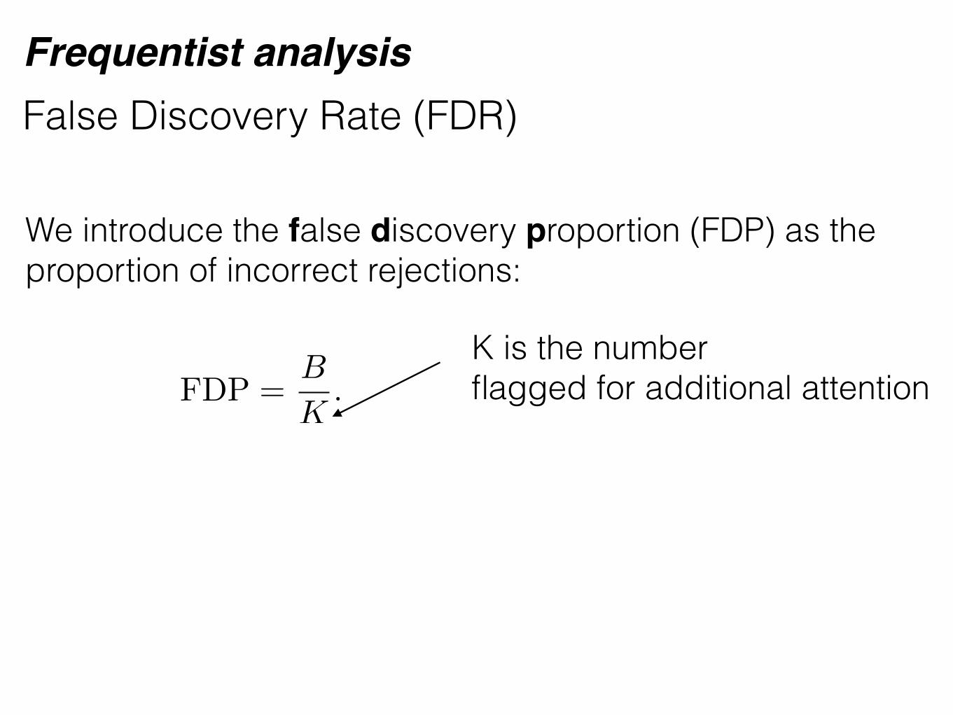
False Discovery Rate (FDR) Frequentist analysis
We introduce the false discovery proportion (FDP) as the proportion of incorrect rejections:
FDP =B
K.
B is the number of type I errors
False Discovery Rate (FDR) Frequentist analysis
We introduce the false discovery proportion (FDP) as the proportion of incorrect rejections:
FDP =B
K.
K is the number flagged for additional attention

False Discovery Rate (FDR) Frequentist analysis
False Discovery Rate (FDR), the expected proportion of rejected nulls that are actually true:
FDR = E [FDP] = E [B/K|K > 0]P (K > 0)

False Discovery Rate (FDR) Benjamini and Hochberg (1995) procedure
Frequentist analysis
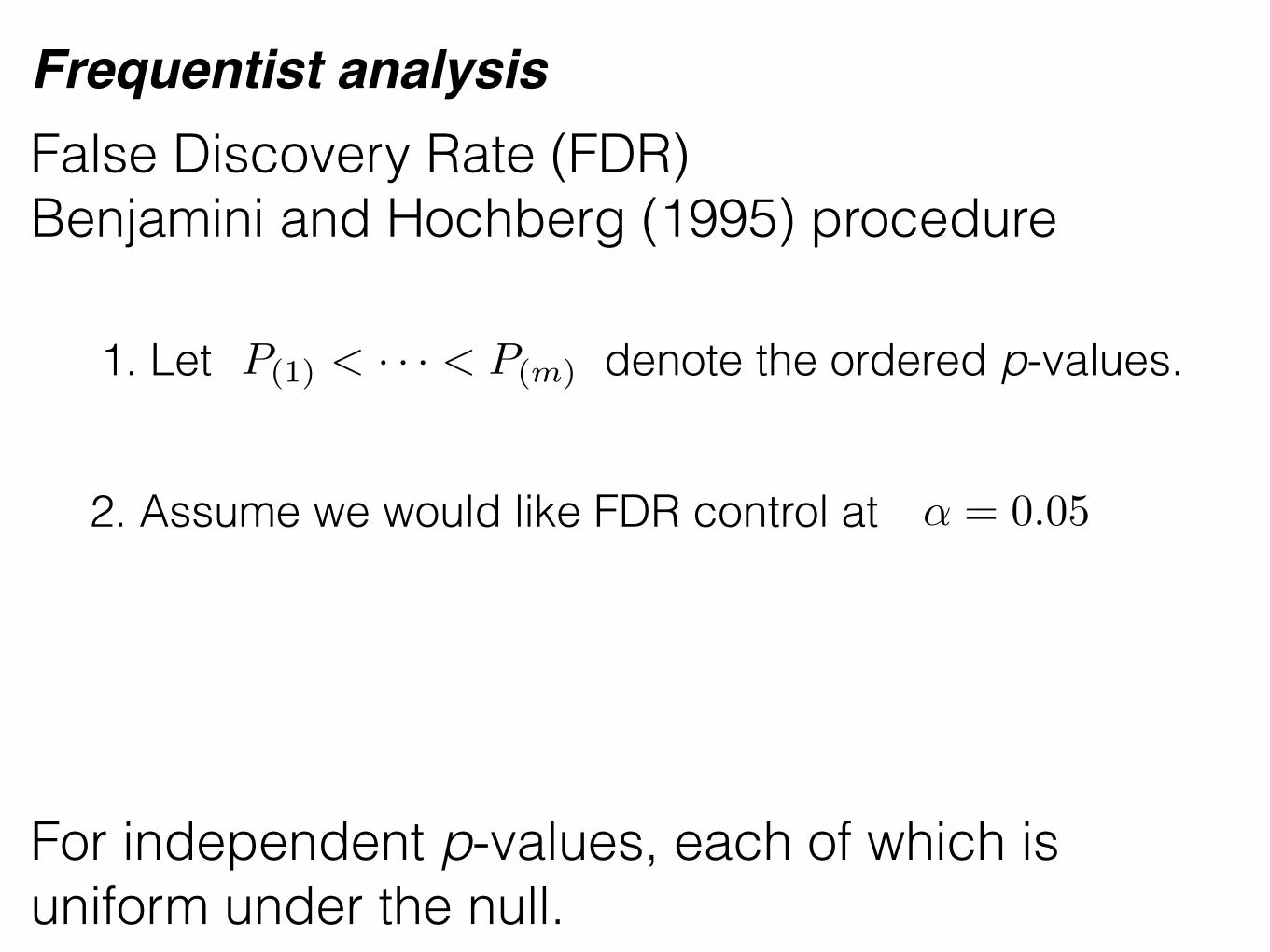
For independent p-values, each of which is uniform under the null.
P(1) < · · · < P(m)1. Let denote the ordered p-values.
False Discovery Rate (FDR) Benjamini and Hochberg (1995) procedure
Frequentist analysis
For independent p-values, each of which is uniform under the null.
P(1) < · · · < P(m)1. Let denote the ordered p-values.
2. Assume we would like FDR control at ↵ = 0.05

False Discovery Rate (FDR) Benjamini and Hochberg (1995) procedure
Frequentist analysisP(1) < · · · < P(m)1. Let denote the ordered p-values.
2. Assume we would like FDR control at ↵ = 0.05
li = i↵/m R = max
�i : P(i) < li
Let and
3. We use p-value threshold at P(R).

False Discovery Rate (FDR) Benjamini and Hochberg (1995) procedure
Frequentist analysis
GWAS example
1. Assume m = 1,000,000 independent tests.2. Assume P(10) = 4.5e-7 and P(11) = 5.7e-7
10*.05/1,000,000 = 5e-7P(10) < 5e-7

False Discovery Rate (FDR) Benjamini and Hochberg (1995) procedure
Frequentist analysis
GWAS example
1. Assume m = 1,000,000 independent tests.2. Assume P(10) = 4.5e-7 and P(11) = 5.7e-7
10*.05/1,000,000 = 5e-7P(10) < 5e-7
11*.05/1,000,000 = 5.5e-7P(11) 5.5e-7⌅

False Discovery Rate (FDR) Benjamini and Hochberg (1995) procedure
Frequentist analysis
GWAS example
1. Assume m = 1,000,000 independent tests.2. Assume P(10) = 4.5e-7 and P(11) = 5.7e-7
10*.05/1,000,000 = 5e-7P(10) < 5e-7
11*.05/1,000,000 = 5.5e-7P(11) 5.5e-7⌅
3. Use p-value threshold at P(10).

False Discovery Rate (FDR) Benjamini and Hochberg (1995) procedure
Frequentist analysis
FDR is controlled at
If procedure is applied, then regardless of how many nulls are true (m0) and regardless of the distribution of the p-values when the null is false
FDR m0
m↵ < ↵.
↵.

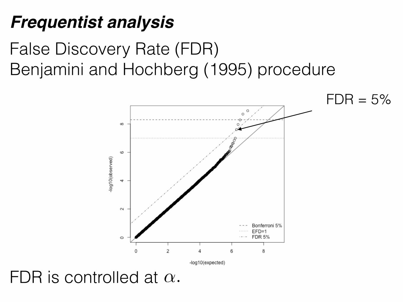
False Discovery Rate (FDR) Benjamini and Hochberg (1995) procedure
Frequentist analysis
FDR is controlled at ↵.
Bonferroni = 5%
False Discovery Rate (FDR) Benjamini and Hochberg (1995) procedure
Frequentist analysis
FDR is controlled at ↵.
FDR = 5%

False Discovery Rate (FDR) Benjamini and Hochberg (1995) procedure
Frequentist analysis
FDR is controlled at ↵.
EFD = 1
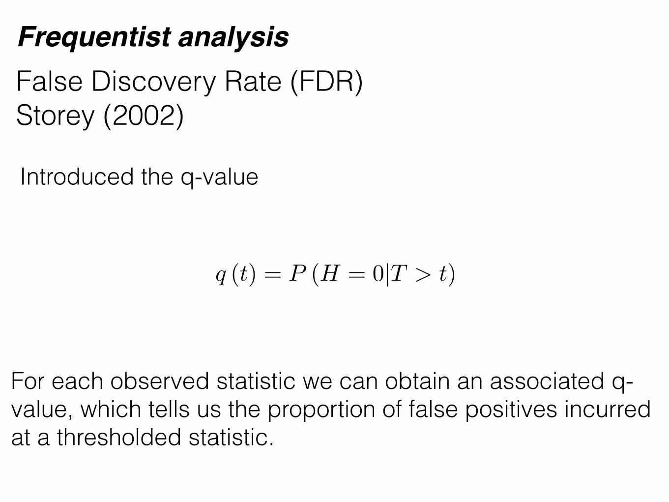
False Discovery Rate (FDR) Storey (2002)
Frequentist analysis
Introduced the q-value
For each observed statistic we can obtain an associated q-value, which tells us the proportion of false positives incurred at a thresholded statistic.
q (t) = P (H = 0|T > t)

In a multiple testing situation there are a variety of criteria that may be considered:
1. Bonferroni method 2. Sidák correction 3. Benjamini and Hochberg (FDR) 4. Storey (FDR)
Frequentist analysis
Bayesian analysis1. Bayesian Bonferroni-type correction2. Mixture models3. Matthew Stephens’ FDR approach

Bayes Factors
Bayesian analysis
Defined as ratios of marginal likelihoods of the data under two models.
Model 0 can be the null model.
Bayes Factori = P (Data|M0) /P (Data|M1)
Bayes Factors
Bayesian analysis
We apply the same procedure m times (can be genetic variants for instance).

Bayes Factors
Bayesian analysis
Combine with prior probabilities
Posterior Oddsi = Bayes Factori ⇥ Prior Oddsi
where
Prior Oddsi = ⇡0i/ (1� ⇡0i) .

Bayes Factors
Bayesian analysis
Combine with prior probabilities
Posterior Oddsi = Bayes Factori ⇥ Prior Oddsi
where
Prior Oddsi = ⇡0i/ (1� ⇡0i) .
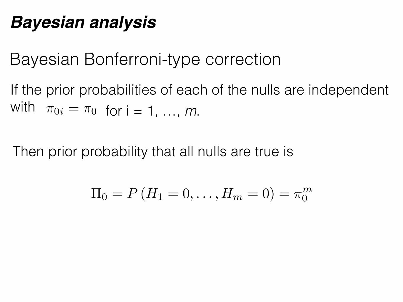
Bayesian Bonferroni-type correction
Bayesian analysis
If the prior probabilities of each of the nulls are independent with ⇡0i = ⇡0 for i = 1, …, m.
Then prior probability that all nulls are true is
⇧0 = P (H1 = 0, . . . , Hm = 0) = ⇡m0
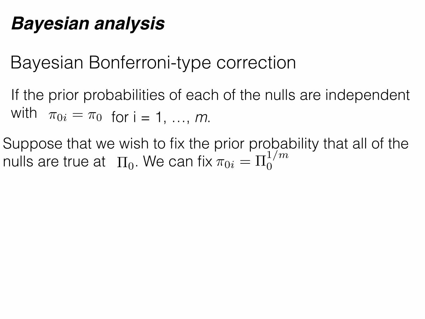
Bayesian Bonferroni-type correction
Bayesian analysis
If the prior probabilities of each of the nulls are independent with ⇡0i = ⇡0 for i = 1, …, m.
Suppose that we wish to fix the prior probability that all of the nulls are true at . We can fix ⇧0 ⇡0i = ⇧1/m
0
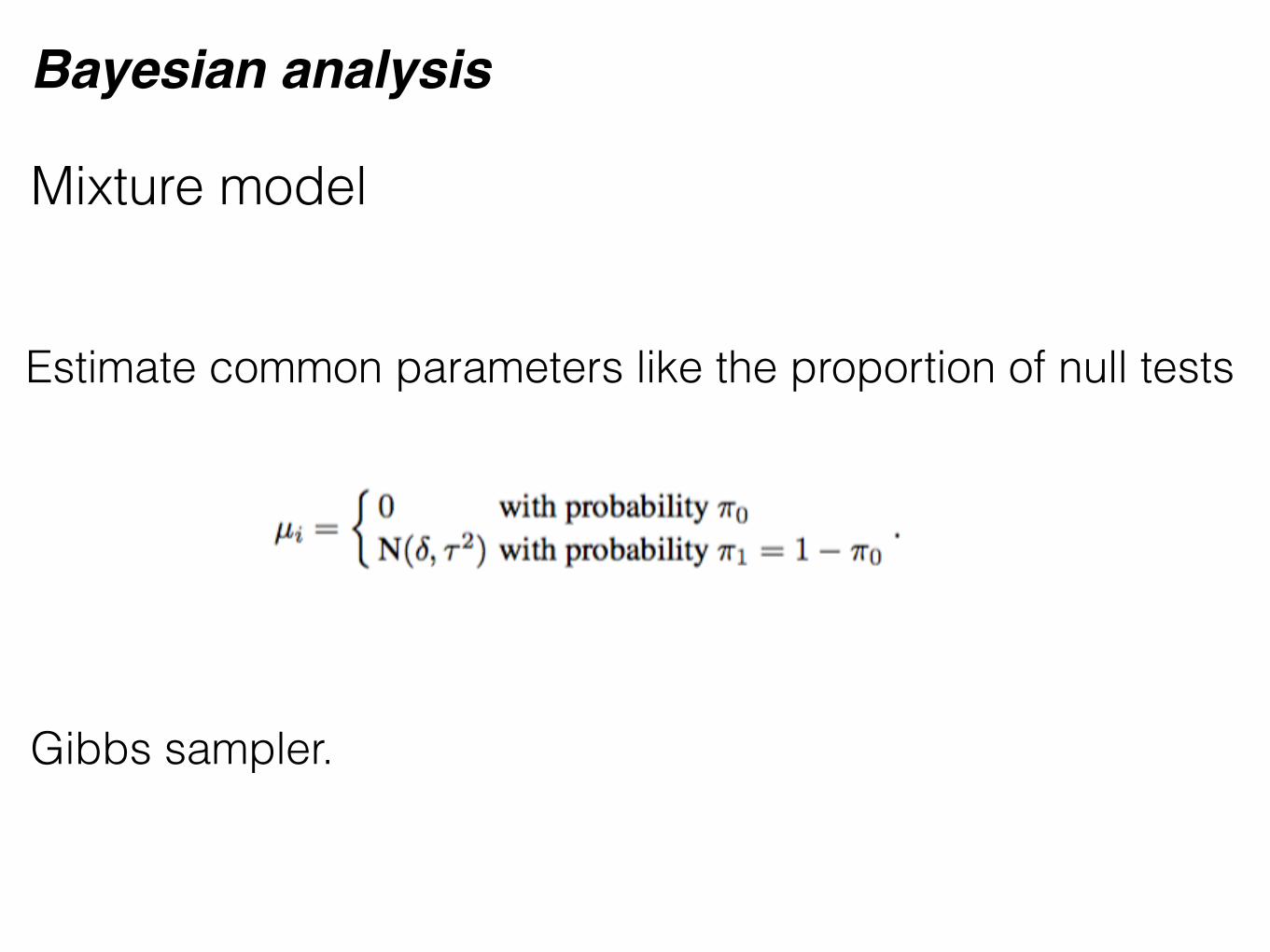
Mixture model
Bayesian analysis
Estimate common parameters like the proportion of null tests
Gibbs sampler.

Matthew Stephens’ FDR approach
Bayesian analysis
Matthew Stephens’ FDR approach
Bayesian analysis
Open source R package
http://github.com/stephens999/ashr
ashr

Matthew Stephens’ FDR approach
Bayesian analysis
Three key ideas
1. Assumes distribution of effects is unimodal, with a mode at 0.

Matthew Stephens’ FDR approach
Bayesian analysis
Three key ideas
1. Assumes distribution of effects is unimodal, with a mode at 0.
2. Takes as input two numbers: i) effect size estimate and ii) corresponding standard error.
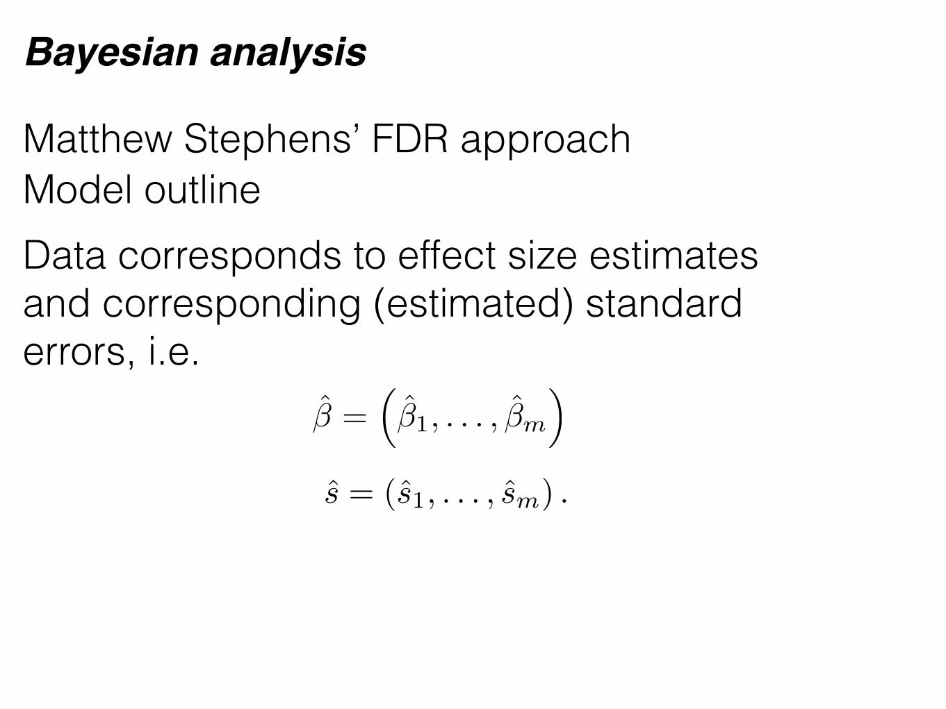
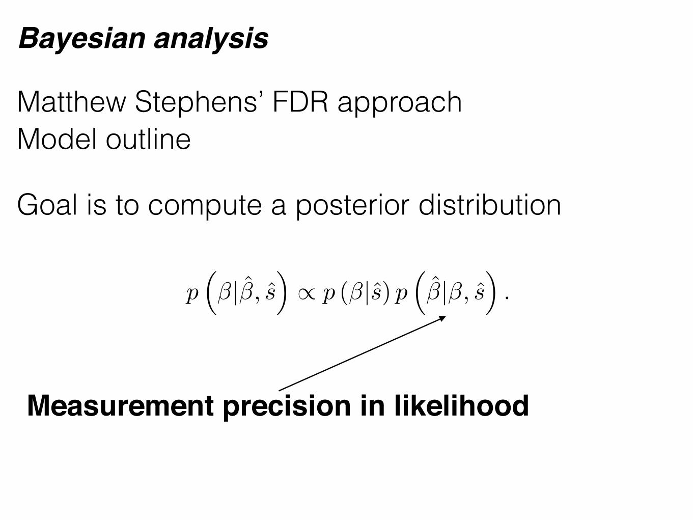
Matthew Stephens’ FDR approach
Bayesian analysis
Model outlineData corresponds to effect size estimates and corresponding (estimated) standard errors, i.e.
� =⇣�1, . . . , �m
⌘
s = (s1, . . . , sm) .

Matthew Stephens’ FDR approach
Bayesian analysis
Model outline
Goal is to compute a posterior distribution
p⇣�|�, s
⌘/ p (�|s) p
⇣�|�, s
⌘.
LikelihoodPrior

Matthew Stephens’ FDR approach
Bayesian analysis
Model outline
Goal is to compute a posterior distribution
p⇣�|�, s
⌘/ p (�|s) p
⇣�|�, s
⌘.
Key: For assumption is that the betas are independent from a unimodal distribution.
p (�|s)
“Unimodal assumption”
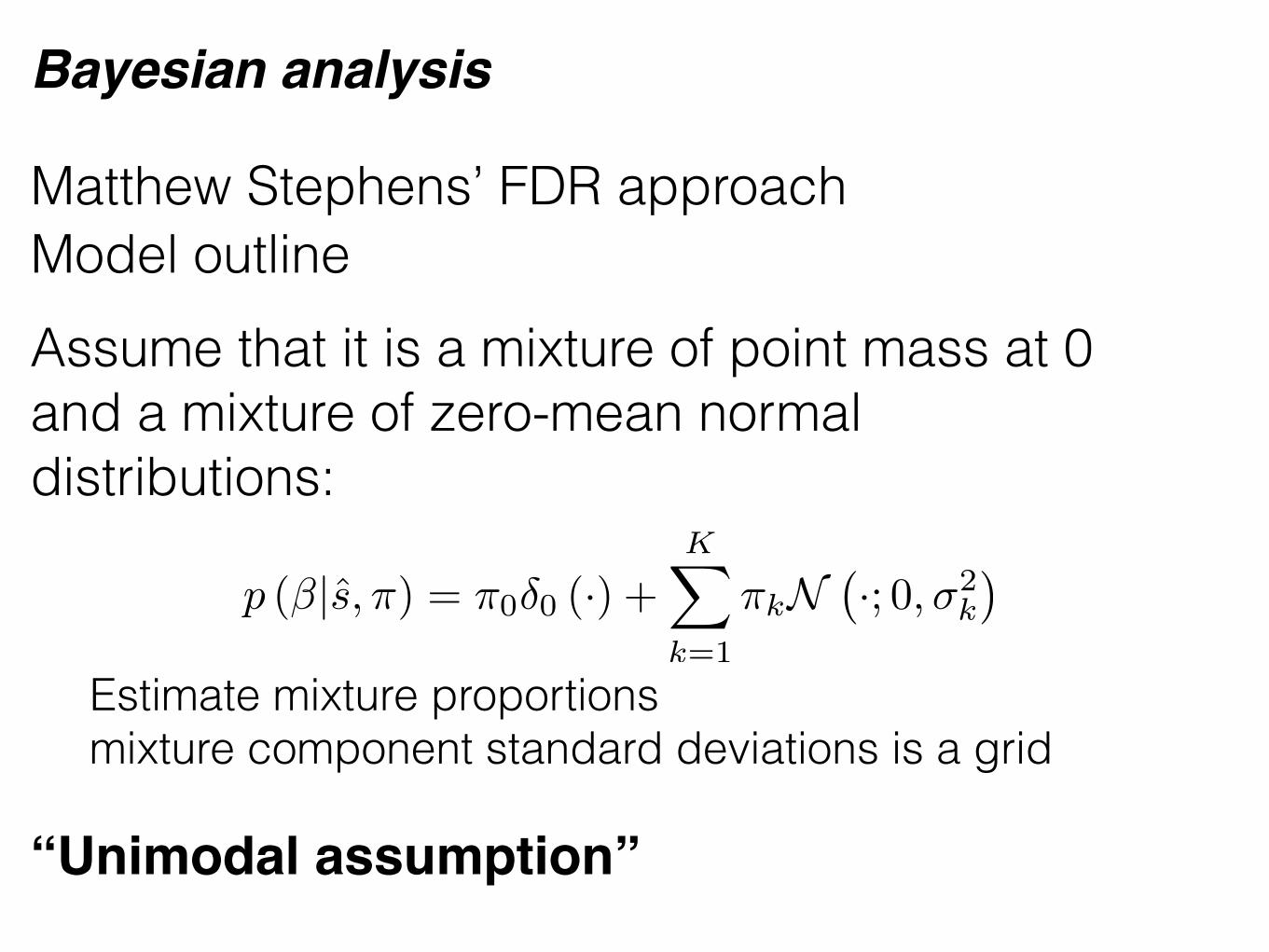
Matthew Stephens’ FDR approach
Bayesian analysis
Model outlineAssume that it is a mixture of point mass at 0 and a mixture of zero-mean normal distributions:
“Unimodal assumption”
p (�|s,⇡) = ⇡0�0 (·) +KX
k=1
⇡kN�·; 0,�2
k
�
Estimate mixture proportions mixture component standard deviations is a grid

Matthew Stephens’ FDR approach
Bayesian analysis
Model outline
For the likelihood p⇣�|�, s
⌘
p⇣�|�, s
⌘=
mY
j=1
N⇣�j ;�j , s
2j
⌘

Matthew Stephens’ FDR approach
Bayesian analysis
Model outline
Goal is to compute a posterior distribution
p⇣�|�, s
⌘/ p (�|s) p
⇣�|�, s
⌘.
“Unimodal assumption”
Matthew Stephens’ FDR approach
Bayesian analysis
Model outline
Goal is to compute a posterior distribution
p⇣�|�, s
⌘/ p (�|s) p
⇣�|�, s
⌘.
Measurement precision in likelihood

Matthew Stephens’ FDR approach
Bayesian analysis
Three key ideas
1. Assumes distribution of effects is unimodal, with a mode at 0.
2. Takes as input two numbers: i) effect size estimate and ii) corresponding standard error.
3. local false sign rate - probability of getting sign of effect wrong.
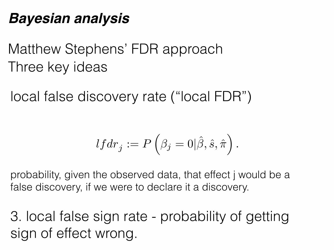
Matthew Stephens’ FDR approach
Bayesian analysis
Three key ideas
3. local false sign rate - probability of getting sign of effect wrong.
lfdrj := P⇣�j = 0|�, s, ⇡
⌘.
local false discovery rate (“local FDR”)
probability, given the observed data, that effect j would be a false discovery, if we were to declare it a discovery.
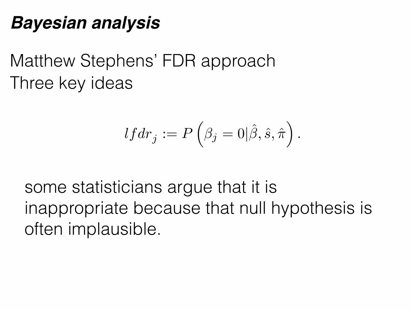
Matthew Stephens’ FDR approach
Bayesian analysis
Three key ideas
lfdrj := P⇣�j = 0|�, s, ⇡
⌘.
some statisticians argue that it is inappropriate because that null hypothesis is often implausible.
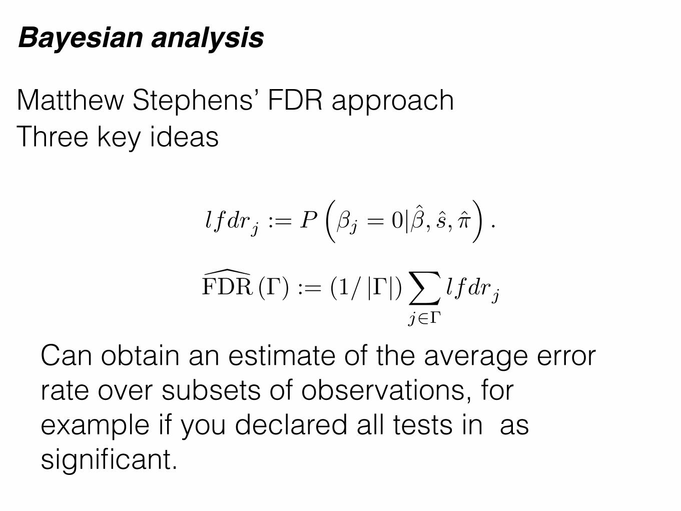
Matthew Stephens’ FDR approach
Bayesian analysis
Three key ideas
lfdrj := P⇣�j = 0|�, s, ⇡
⌘.
Can obtain an estimate of the average error rate over subsets of observations, for example if you declared all tests in as significant.
[FDR (�) := (1/ |�|)X
j2�
lfdrj

Matthew Stephens’ FDR approach
Bayesian analysis
Three key ideas
Tukey stated:
All we know about the world teaches us that the effects of A and B are always different - in some
decimal place - for any A and B.

Matthew Stephens’ FDR approach
Bayesian analysis
Three key ideas
3. local false sign rate - probability of getting sign of effect wrong.
Tukey suggested:
Is the evidence strong enough to support a belief that the observed difference has the correct sign?

Matthew Stephens’ FDR approach
Bayesian analysis
Three key ideas3. local false sign rate - probability of getting sign of effect wrong.
lfsrj := minhp⇣�j � 0|�, s
⌘, p
⇣�j 0|⇡, �, s
⌘i.

Matthew Stephens’ FDR approach
Bayesian analysis
Three key ideas3. local false sign rate - probability of getting sign of effect wrong.
lfsrj := minhp⇣�j � 0|�, s
⌘, p
⇣�j 0|⇡, �, s
⌘i.
Gelman proposed focusing on “type S errors”, errors in sign, rather than traditional type I errors.
Matthew Stephens’ FDR approach
Bayesian analysis
Other results/observations covered, but not in this primer
1. Computation/Implementation details 2. Comparisons to other approaches

Multiple tests of the same null hypothesis
Bayesian analysis
In genetics we may be interested in applying: 1) additive model, 2) dominant, and 3) recessive model.
How to correct?

Multiple tests of the same null hypothesis
Bayesian analysis
In genetics we may be interested in applying: 1) additive model, 2) dominant, and 3) recessive model.
Bonferroni?
Multiple tests of the same null hypothesis
Bayesian analysis
In genetics we may be interested in applying: 1) additive model, 2) dominant, and 3) recessive model.
Bonferroni? Too conservative.
Multiple tests of the same null hypothesis
Bayesian analysis
In genetics we may be interested in applying: 1) additive model, 2) dominant, and 3) recessive model.
Minimum p-value?
Multiple tests of the same null hypothesis
Bayesian analysis
In genetics we may be interested in applying: 1) additive model, 2) dominant, and 3) recessive model.
Minimum p-value? not valid p-value since it is not uniform under the null. (can modify null though)

Multiple tests of the same null hypothesis
Bayesian analysis
In genetics we may be interested in applying: 1) additive model, 2) dominant, and 3) recessive model.
Minimum p-value? not valid p-value since it is not uniform under the null.
Permutation.

Multiple tests of the same null hypothesis
Bayesian analysis
In genetics we may be interested in applying: 1) additive model, 2) dominant, and 3) recessive model.
Bayesian model averaging.
Hoeting, Madigan, Raftery and Volinksy Statisticial Science 1999
Recommended