Articleshttps://doi.org/10.1038/s41559-017-0383-4
© 2017 Macmillan Publishers Limited, part of Springer Nature. All rights reserved.
The architecture of mutualistic networks as an evolutionary spandrelSergi Valverde 1,2,3*, Jordi Piñero1,2, Bernat Corominas-Murtra4,5, Jose Montoya6, Lucas Joppa7 and Ricard Solé1,2,8*
1ICREA-Complex Systems Lab, Universitat Pompeu Fabra, Dr Aiguader 88, 08003 Barcelona, Spain. 2Institute of Evolutionary Biology (CSIC-UPF), 37–49 Passeig de la Barceloneta, 08003 Barcelona, Spain. 3European Centre for Living Technology, San Marco 2940, 30124 Venice, Italy. 4Section for the Science of Complex Systems, CeMSIIS, Medical University of Vienna, Spitalgasse 23, A-1090 Vienna, Austria. 5Vienna Complexity Science Hub, Josefstadterstrasse 39, 1080 Vienna, Austria. 6Theoretical and Experimental Ecology Station, CNRS-University Paul Sabatier, Moulis 09200, France. 7Microsoft Research, Cambridge CB1 2FB, UK. 8Santa Fe Institute, 1399 Hyde Park Road, Santa Fe, NM 87501, USA. *e-mail: [email protected]; [email protected]
SUPPLEMENTARY INFORMATION
In the format provided by the authors and unedited.
NaTuRe eCoLogy & eVoLuTioN | www.nature.com/natecolevol

Contents
I. Networks and Network Dataset 3
II. Topological network model 7
A. Mean Field Theory 9
B. Stationary degree distribution 12
III. Network nestedness: Estimation of spectral radius 16
Nestedness over S for the random network 18
IV. References 19
References 19
2

I. NETWORKS AND NETWORK DATASET
As a benchmark for our study, we have used a database of ecological networks from the
NCEAS site (https://www.nceas.ucsb.edu/interactionweb/). Specifically, we have used the
three datasets involving mutualistic interactions, namely plant-ant, plant-herbivore and plant-
pollinator webs along with two webs associated to anemone-fish interactions. This set includes a
range of network sizes with a very diverse class of plant-animal assemblies. The full description
of each dataset, including original publication, habitat type, location and size (number of species
in each layer) is provided in: https://www.nceas.ucsb.edu/interactionweb/resources.html.
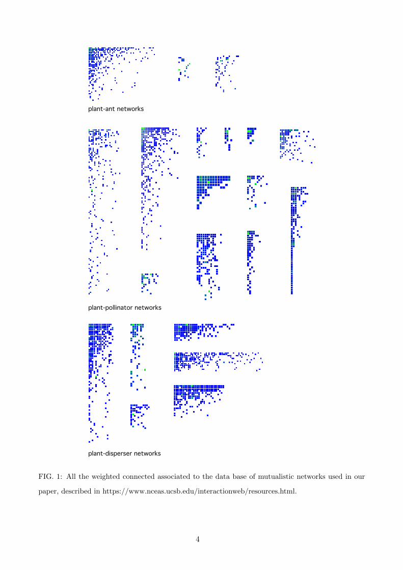
The data base includes many webs, but here we only use those that include the weights
of the interactions associated with each mutualistic association. These constitute a total of
25 networks, of which only 21 are fully connected. The weight of links has been determined
by means of the number of visits. The size of these networks varies widely from very small
(S ∼ 10) to relatively large (S ∼ 102). In Figure 1 the adjacency matrices are displayed for each
connected web, in order to illustrate the presence of nested patterning as well as its variability.
3
plant-ant networks
plant-pollinator networks
plant-disperser networks
FIG. 1: All the weighted connected associated to the data base of mutualistic networks used in our
paper, described in https://www.nceas.ucsb.edu/interactionweb/resources.html.
4

10-2 10-1 100 10110-2
10-1
100
100 101 10210-2
10-1
100
k/kc
k
P>
(k)
k�P
(k)
FIG. 2: This figure shows the structural behaviour of 6 of the real data sets, such that S ≥ 65. As
discussed in Jordano et al ((27) in the main text), this method shows that mutualistic networks follow
truncated power laws. The inset shows the comulative degree distributions before collapsing the data
under the scaling ansatz.
5

6

100 101 102
10-4
10-3
10-2
10-1
100
0 1 2 30
0.2
0.4
0.6
s(k)
k
⌘P
(⌘)
FIG. 3: This figure shows the scaling behaviour of the memmott network data for the strength against
the degree, k. The predicted exponent for this particular network is η = 1.50. The inset corresponds
to the normalized histogram of all the estimated exponents for the 25 real networks. Comparison
bewteen this figure and Figures 3a-b (in the main text) reveals the strong affinity between real data
and in silico generated networks from our model.
II. TOPOLOGICAL NETWORK MODEL
In this section we introduce a topological model for the growth dynamics of a bipartite
network. This model ignores the weights of the links and the threshold conditions associated to
both saturation and edge removal used in the main text. The weighted graph model is capable of
accounting for all the relevant features exhibited by real graphs where the relative importance
of each pairwise interaction have been estimated. There are two reasons for considering an
additional, non-weighted approach. The first is the difficulty to define a formal model involving
weighted links. The second is whether such a model is capable of capturing similar structural
trends, while comparing with the more accurate computational model.
In the weighted model, the loss of links under the threshold condition and the requirement
of a maximal number of links per node are important components of the rules. They provide
7

a mechanism for regulating the number of links per species and limits connection growth.
Network growth can be classified into a limited number of universality classes (1). The distinct
models characterized by the same universality class share several key fundamental properties as
reflected by the nature of the different phases they belong to. This is actually at the core of our
main message: beyond the specific details that can be included in a model, statistical physics
reveals an understanding of the coarse emerging patterns by considering only the underlying
skeleton of the interactions.
Since a topological counterpart will use a binary description of edges, the topological rules
will be necessarily different. The model will need to incorporate specific rules preserving the
essence of the duplication-rewiring mechanism while limiting the rate of link growth. Several
potential sets of rules can be considered. Here we explore the simplest set-up, which rules are
summarized in Figure 2.
Our bipartite network will be again a graph G(A,P, ω), such that A∪P is the set of all the
nodes of G, with the property that any given edge ωij ∈ ω links an element Ai ∈ A with an
element Pj ∈ P . Now, only two states are allowed for an edge, i.e., ωij ∈ {0, 1}, representing
absence or presence, respectively.
Let us introduce the model’s iterative rules:
(i) Begin iteration by choosing at random one of the two sets. Each subset µ = A,P will be
chosen with probability πµ such that∑
µ πµ = 1 .
(ii) As in the weighted model, duplicate a random element of the selected subset and ran-
domly delete duplicated links with probability δ.
(iii) Attach new edges to the duplicated element with probability α. Since our topological
model does not include a threshold condition that effectively limits the number and influence
of links, the probability introduced here will be affected inversely by the system size.
(iv) Return to (i) and repeat the sequence.
Using the rules above, we will derive a mean field theory that provides an estimate of
the average connectivity. As shown below, the average degree of these webs is a well-defined
function of the two key parameters associated to the duplication-divergence rules described
above. Additionally, the model also predicts a scaling law connecting the number of species S
and links L that is consistent with the observed in real webs and in the weighted model (as
shown in Figure 4, main text).
Moreover, the stationary degree distribution will also be determined by using a master
8

equation expansion and its stationary solution. This distribution is shown to display a truncated
power law behaviour, with specific predictions about the relevant parameters affecting the
scaling decay and its corresponding cut-off.
A. Mean Field Theory
The first step in our mathematical analysis is to determine how the connectivity scales with
species diversity. The observed data set (Figure 2b, main text) indicates that we should expect
a scaling law with the total number of species S = |A ∪ P |,
L ∼ S σ , (1)
that ranges between 1 < σ < 2. Notice that the network construction process is such that
S exactly corresponds to the time-step counter for the algorithm. The following analysis cor-
responds to a coarse-grained gauge of the bounds for σ. However, its predictions accurately
reflect the measurements from the fully computationally implemented model.
Taking into account the iteration process described above, let us try to formalize a minimal
model supposing that all network nodes are equally connected and in a highly mixed state. In
this mean field approach the following equation holds:
L(S) = Kµ(S)Sµ(S) =S
2
⟨K⟩π, (2)
where, Sµ = |µ|, with µ ∈ {A,P} . By construction, Sµ(S) = πµS, and we define
⟨K⟩π
:=∑µ
πµKµ .
From the algorithm rules, the following discrete dynamical equation is derived:
L(S + 1) = L(S) +∑µ
πµKµ − δ∑µ
πµKµ + α∑µ
πµ(Sµ −Kµ
), (3)
where we denote µ as the complementary subset of µ, i.e., A = P and P = A. We can transform
our discrete dynamical model into a continuous one through the approximation:
dL
dS' L(S + 1)− L(S) , (4)
which in our case reads:
dL
dS' (1− δ − α)
⟨K⟩π
+ 2απAπPS . (5)
9

A
P
P1 P2
A2A1 A3
A
P P1 P2
A2A1 A3 A4
A
P P1 P2
A2 A3 A4
A
PP1 P2
A2A1
P3
A3
⇡a ⇡p
� �
A1
P3
P3
P3
!
A
P P1 P2
A2 A3 A4A1
P3
↵
P4
A
PP1 P2
A2A1
P3
A3
P4
↵
A
PP1 P2
A2A1
P3
A3
P4
Spec
iatio
nDive
rgen
ce
FIG. 4: A summary of the rules applied to the topological model of bipartite graph evolution. Starting
from a given initial, small graph, we choose either A or P and a random species that becomes dupli-
cated. This occurs with probabilities πA (left) and πP = 1− πA (right). Afterwards, with probability
δ the redundant links can be deleted and finally, with some probability α, additional connections are
introduced.
10

At this point, we introduce a regulator on the attachment process by introducing a size-
dependent control of addition rate, which we choose to be an inverse of S, i.e., α = β/S.
This relationship provides one possible way of reducing the growth rate of connections that is
naturally present in the weighted model but needs to be introduced here. This kind of approach
has been used in the context of proteome evolution models (2,3). Other possibilities can be
used (4) by simply limiting the number of links to a small subset. It can be argued that a
diversity-dependent rule is a simple way of providing a limit to connectivity explosions, which
(in a dynamical scenario) would destabilise the ecosystem.
Under this premises, the following differential equation is derived for the evolution of the
number of links in the network,
dL
dS= 2(1− δ)L
S− 2β
L
S2+ 2βπAπP , (6)
which is now a differential equation with S as time and which general solution is given by
L(S) = S2(1−δ)e2β/S[C + πAπP (2β)2δΓ
(1− 2δ, 2β/S
)]. (7)
Henceforth, two phases for the growth of the bipartite network emerge, each with a charac-
teristic scaling law between the number of links and the total number of network nodes,
L ∼
S2(1−δ) 0 < δ < 1
2
S 1 > δ > 12.
(8)
In this model, when the deletion probability δ < 12, the duplication process, here generated
by (i)-(ii), is the dominant growth mechanism, while for greater values of δ the reattachement
process, (iii), becomes the dominant dynamics. These two mechanisms are characterised by the
two dynamical exponents found in eq. (9).
This is the main result of our analysis in this section. It provides a well defined prediction
for the scaling law L ∼ Sσ, consistent with the observed data sets and the weighted model
distributions. For high deletion rates, a lower bound of the model is given by a linear relation
(i.e. σ = 1) and for lower δ values the scaling exponent is bounded from above by σ = 2
(δ = 0). Shift from one behaviour to the other continuously transitions at δc = 1/2.
A complementary result is also obtained by computing the average connectivity:
Kµ ∼
S1−2δ 0 < δ < 1
2
K∗µ 1 > δ > 12,
(9)
11
where we have defined K∗µ as
K∗µ =2βπµ
2δ − 1. (10)
Provided that the system’s replication choice is taken to be symmetric, i.e., πA = πP = 12,
the average expected degree for δ > 12
becomes
K∗A = K∗P =β
2δ − 1. (11)
Here onwards we will only consider this particular symmetrical case. A better and more com-
plete description of the steady state properties of a network experiencing growth is conveyed
by the degree distribution. In the following section we derive this distribution and study its
emergent structure.
B. Stationary degree distribution
The network degree distribution pk provides a better characterisation of the network organ-
isation, beyond the average measures such as mean degree. It also reveals key features of the
network, in particular, the presence of scaling laws or cut-offs. As discussed in the main article,
available data reveal that mutualistic webs display distributions of connections that are more
complex than a simple exponential. Instead, they tend to be broad while exhibiting marked
cut-offs.
Let us begin by considering the network’s population degree, that is the number of nodes in
either subset A or P attached to k edges, nµk . Owing to symmetry, nAk = nBk ≡ nk. However, in
order to introduce the transition probabilities we will start by regarding the general problem
and later restrict the analysis to the symmetrical subset choice.
Now, as mentioned before, the time-step of the algorithm scales with the number of nodes
of the full network, t ∼ S since a new node is generated per iteration.
To proceed with a master equation first we require to ennumerate all the possible transitions
between degree populations at each iteration
1. Probability of simple increase of the kth−population
P [nµk → nµk + 1] = πµnµkSµ
(1− kδ) + πµnµk+1
Sµ(k + 1)δ , (12)
where the first term stands for the probability of replication of an element of nµk without
any removal, while the second considers replication of a member from the nµk+1 population with
subsequent removal process of a single edge, thus adding a member to nµk .
12

2. Probability of increase of the kth−population with elimination of a member of the (k −1)th−population
P [(nµk−1, nµk)→ (nµk−1 − 1, nµk + 1)] = πµ
nµk−1
Sµ(k − 1)(1− δ)
+ αnµk−1
Sµ(πµSµ + πµSµ) . (13)
Here, the first term corresponds to replication on the complementary subset with subsequent
duplication of an edge on the µ’s (k − 1)th−population (without removal); plus probability of
reattachement of an edge to a member of nµk−1. Notice that we approximate the latter by
considering it to be decoupled from the previous step of duplication.
Under the self-regulating ansatz for α,
αnµk−1
Sµ(πµSµ + πµSµ)→ 2βπµπµ
nµk−1
Sµ.
Focusing our analysis on the symmetrical case for subset choice probability, πA = πP = 1/2,
we study the variation of the degree-population of any subset,
dnkdt∼ dnk
dS= P [nk → nk + 1] + P [(nk−1, nk)→ (nk−1 − 1, nk + 1)]
−P [(nk, nk+1)→ (nk − 1, nk+1 + 1)]
=1
2pk(1− kδ) +
1
2pk+1(k + 1)δ +
1
2pk−1(k − 1)(1− δ)
+β
2pk−1 −
1
2pkk(1− δ)− β
2pk , (14)
where pk ≡ pAk = pBk ≡nµkNµ
= nkS/2
, i.e., pk is the degree distribution. Moreover, let us consider
that given a sufficiently large number of iterations, the distribution will become stationary.
Thus,
dpµkdt∼ dpµk
dS=
1
S
dnµkdS− pµkS
= 0 , (15)
therefore,
δ(k + 1)pk+1 + (1− δ)(k − 1)pk−1 − kpk + β(pk−1 − pk) = 0 . (16)
To solve this recursive equation, it is convenient to define a genereting function as follows:
φ(z) :=∑k≥0
pkzk , pk =
1
k!
dkφ
dzk
∣∣∣z=0
. (17)
Using probability normalization we obtain the boundary condition φ(1) = 1, while eq. (16)
becomes: [δ − z + (1− δ)z2
]dφdz
= β(1− z)φ(z) . (18)
13

Both sides of eq. (18) contain the root (1− z), thus, it can be reduced to
[δ − (1− δ)z
]dφdz
= βφ(z) , (19)
which leads to
φ(z) =(δ − (1− δ)z
2δ − 1
)− β1−δ
. (20)
From eq. (20) it is possible to extract some network measures such as the average degree
〈k〉 =∑k≥0
kpk = zdφ
dz
∣∣∣z=1
=β
2δ − 1, (21)
which corresponds to the mean field prediction for the symmetric case, eq. (11). On the other
hand, we can derive the degree distribution using eq. (17):
pk =1
k!
( δ
2δ − 1
)− β1−δ(1− δ
δ
)kΓ( β
1− δ + k)[
Γ( β
1− δ)]−1
(22)
In order to write down the previous equation in a more simple form, we introduce the Stirling
approximation for large degree values. The final result takes the familiar form of a truncated
power law:
pk ∼ (k0 + k)−γe−k/kc (23)
where the constants are given by the parameter combinations:
k0 =β
1− δ (24)
γ = 1− β
1− δ (25)
kc =1
log(
δ1−δ
) (26)
This distrbution may be normalized by taking the continuum limit as follows [1]:
∑k≥0
(k0 + k)−γe−k/kc →∫ ∞
0
(k0 + x)−γe−x/kcdx = e−k0/kc∫ ∞k0
t−γe−t/kc
= e−k0/kcΓ (1− γ, k0) = e−k0/kcΓ (k0, k0)
Finally, let us make some remarks in regards of this model. First notice how, if condition
δ > 1/2 is not met, then eq. (21) would not be well defined. The reason behind it is that, in
14

such circumstances, the system would not acquire a steady state and eq. (15) would no longer
hold.
Furthermore, previous results behave accordingly with the set of rules for the network
genereting model regarding the shift of the degree cuttoff (kc) and how the exponent γ is
expected to shift depending on the reattachement rate β. Alternative derivations of degree
distribution for generated networks have been put forward using clustering properties (5).
15

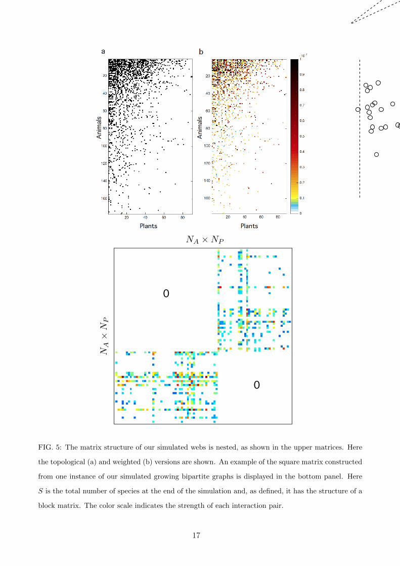
III. NETWORK NESTEDNESS: ESTIMATION OF SPECTRAL RADIUS
Let SA = |A| be the number of animal species and SP = |P | be the number of plant species,
i.e., the total number of species in our system is S = SA + SP . Now, assume that animals are
indexed 1, 2, .., SA and plants are labeled SA + 1, SA + 2, ..., SA +SP . The matrix of mutualistic
interactions ω = [ωij] has a block off-diagonal form like this:
ω =
0 ωSA×SP
ωSP×SA 0
=
0 BT
B 0
(27)
where 0 represents an all-zero matrix, indicating that there are no interactions between any
pair of alike species; and B is the incidence matrix (see (16) in the main text). Nestedness is
a relative value that depends on the size (number of species S) and the matrix fill (density of
interactions) of the bipartite matrix. In order to allow a comparison of different systems, it is
necessary to compute the normalized incidence matrix as follows:
B −→ B∑ij Bij
(28)
Now we are able to compute the spectral radius ρ(ω) as the largest eigenvalue associated to
the matrix ω. As shown by (16), this represents a natural natural measurement of nestedness:
large values of ρ(ω) will correspond to highly nested matrices and viceversa.
To assess the relevance of this measurement we compare the observed value of nestedness in
the model with an ensemble of random matrices with similar properties, (7,8). Here, we use the
null model proposed by (16), which keeps the structural features of the network while swapping
the order of weighted links (so-called ’binary shuffle’ in (8)). We assess the significance of
empirical nestedness with the Z-score:
Z =ρ(ω)− 〈ρ〉
σρ(29)
where 〈ρ〉 and σρ are the average value and the standard deviation of the network measure in
a random ensemble, respectively. Here, we consider that mutualistic networks are significantly
nested whenever the corresponding Z > 2 (i.e., p < 0.05 using the Z-test).
16
hki < 2hki > 2
hki=
1
hkiAverage network degree
L ⇠ S
L⇠ S
2
⇢(!
)
hki
0
0
NA ⇥ NP
NA⇥
NP
FIG. 5: The matrix structure of our simulated webs is nested, as shown in the upper matrices. Here
the topological (a) and weighted (b) versions are shown. An example of the square matrix constructed
from one instance of our simulated growing bipartite graphs is displayed in the bottom panel. Here
S is the total number of species at the end of the simulation and, as defined, it has the structure of a
block matrix. The color scale indicates the strength of each interaction pair.
17

Nestedness over S for the random network
Finally, we compare the diversity revealed by our model with the simplest null-model, the
large random network (9). A characteristical feature for this kind of systems is that they show
a well defined average degree. This implies that the scaling behaviour between L and S for
such networks is given by L ∼ S.
On the other hand, summation over all adjacency matrix elements correspods to L =∑
ij Aij.
Therefore, the process of normalization for the random matrix comes with an overall factor of
1/S.
As shown by Wigner (9), for sufficiently large S, the maximal eigenvalue for this system
scales as λM ∼√S. Which, upon reescaling of the matrix by the normalization factor, will
yield:
λ′M ∼ S −12 (30)
Figure 4b (main text) displays this scaling prediction against the largest eigenvalues (ρ(ω)) for
each of the m = 4000 generated networks, plus the 25 real data points from the sources in the
first section of this SM.
18

IV. REFERENCES
1. Dorogovtsev, S. N., Mendes, J. F. F. (2003). Evolution of Networks. Oxford U. Press.
2. Sole, R.V., Pastor-Satorras, R., Smith, E., Kepler, T. (2002). A model of large-scale
proteome evolution. Adv. Complex Syst. 5, 43-54.
3. Pastor-Satorras, R., Smith, E., R., Sole, R.V., (2003). Evolving protein interaction net-
works through gene duplication. J. Theoretical Biology. 222, 199-210.
4. Vazquez, A., Flammini, A., Maritan, A., Vespignani A. (2003). Modeling of Protein
Interaction Network. ComPlexUs. 1, 38-44.
5. Kim, J., Kahng, B., Krapivsky, P.L., Redner, S. (2002). Infinite-Order Percolation and
Giant Fluctuations in a Protein Interaction Network. 2002. Phys. Rev. E. 66, 055101.
6. Abramowitz, M. and Stegun, I. (1964) Handbook of Mathematical Functions. Dover Pub-
lications, New York.
7. Weitz, J. S., Poisot, T., Meyer, J. R., Flores, C. O., Valverde, S., Sullivan, M. B.,
Hochberg, M. E. (2013). Phage-bacteria infection networks. Trends in Microbiology
21(2), 82-91.
8. Beckett, S., Boulton, C.A., Williams, H. T. P. (2014). FALCON: a software package for
analysis of nestedness in bipartite networks. Nature, 500, 449-452.
9. Wigner, E.P. (1955). Characteristic vectors of bordered matrices with infinite dimensions.
Ann. of Math 62, 548-564.
[1] Γ(s, x) stands for the Incomplete Gamma function. See (6).
19
Recommended