The Copula GARCH model for time
varying betas in the banking sector.
INTERNATIONAL HELLENIC UNIVERSITYMaster of Science dissertation
byDimitris Nikolaidis
Dissertation Director: Dr. Markellos
August 2010
Contents
I The First Part - Statistical analysis of copulas 1
1 Introduction to Copulas 2
1.1 Intuition behind copulas. Measures of dependence . . . . . . . . . . . 2
1.1.1 Rank based measures of dependence . . . . . . . . . . . . . . 5
1.2 Definitions and fundamental properties . . . . . . . . . . . . . . . . . 7
1.3 Tail dependence . . . . . . . . . . . . . . . . . . . . . . . . . . . . . . 16
1.4 Inference on copulas . . . . . . . . . . . . . . . . . . . . . . . . . . . 19
1.4.1 Maximum likelihood method . . . . . . . . . . . . . . . . . . . 20
1.4.2 Inference functions for margins (IFM) . . . . . . . . . . . . . . 23
1.4.3 The pseudo likelihood method . . . . . . . . . . . . . . . . . . 25
1.5 Goodness of fit tests for copulas . . . . . . . . . . . . . . . . . . . . . 28
1.5.1 Graphical inspection method . . . . . . . . . . . . . . . . . . . 29
1.5.2 Squared radius method . . . . . . . . . . . . . . . . . . . . . . 31
1.5.3 Bivariate probability integral transform method . . . . . . . . 36
1.6 Conditional Copulas . . . . . . . . . . . . . . . . . . . . . . . . . . . 38
ii
1.6.1 Specifications for the dependence parameters . . . . . . . . . . 39
II The second part - Empirical application 44
2 Introduction 45
2.1 Literature review . . . . . . . . . . . . . . . . . . . . . . . . . . . . . 46
2.2 Data and methodology . . . . . . . . . . . . . . . . . . . . . . . . . . 53
2.2.1 Data and descriptive statistics . . . . . . . . . . . . . . . . . . 56
2.3 Empirical results . . . . . . . . . . . . . . . . . . . . . . . . . . . . . 57
2.3.1 Copula results and time varying parameters . . . . . . . . . . 63
2.3.2 Model comparison and time varying betas . . . . . . . . . . . 65
2.4 Time evolution of betas . . . . . . . . . . . . . . . . . . . . . . . . . 70
2.5 Other copula models . . . . . . . . . . . . . . . . . . . . . . . . . . . 72
2.6 Conclusion . . . . . . . . . . . . . . . . . . . . . . . . . . . . . . . . . 73
iii
Abstract
The Copula GARCH model for time varyingbetas in the banking sector.
Dimitris Nikolaidis
2010
Copula functions have become an increasingly popular tool in finance when the
distribution of asset returns is of extreme importance. The main features of copulas
are that they seperate a multivariate distribution into the dependence structure
and the margins, thus allowing two step estimation procedures for the distributional
parameters that minimize the computational burden and also add flexibility to the
distribution since the dependence governed by the copula and the margins do not have
to belong to the same parametric family, unlike standard multivariate distributions.
The aim of this study is twofold. In the first part, the statistical attributes of
copulas are discussed in full detail while in the second part an empirical investigation
of the evolution of stock betas during the modern global financial crisis period is
conducted. In the empirical part, it is evident that copula models clearly outperform
other, traditional models, in terms of both statistical validity and accuracy in risk
calculations
Part I
The First Part - Statistical
analysis of copulas
1
Chapter 1
Introduction to Copulas
The aim of this chapter is to provide to the reader a rigorous introduction to copulas.
It contains the intuition behind copulas, the main theorems and definitions of the
copula theory, discusses copula inference and presents an overview of the applications
of copulas in finance. For more information, the interested reader is referred to the
books of Joe (1996), Nelsen (2006) or Cherubinni et al. (2004).
1.1 Intuition behind copulas. Measures of depen-
dence
In financial applications the usual measure of dependence is Pearson’s linear corre-
lation. For two random variables X and Y Pearson’s correlation %, is defined as:
% (X, Y ) =cov(X, Y )
σXσY
2
However % measures only linear dependence. It is the correct measure of depen-
dence only in the Gaussian world, that is only if X ∼ N(µ1, σ21) and Y ∼ N(µ2, σ
22).
Linear correlation does not only incorporate information about the dependence of X
and Y but also about their marginal behavior, that is why it is not invariant under
strictly increasing transformations of the data. In other words the linear correlation
of X and Y is different of that of f(X) and g(Y ) for arbitrary strictly increasing
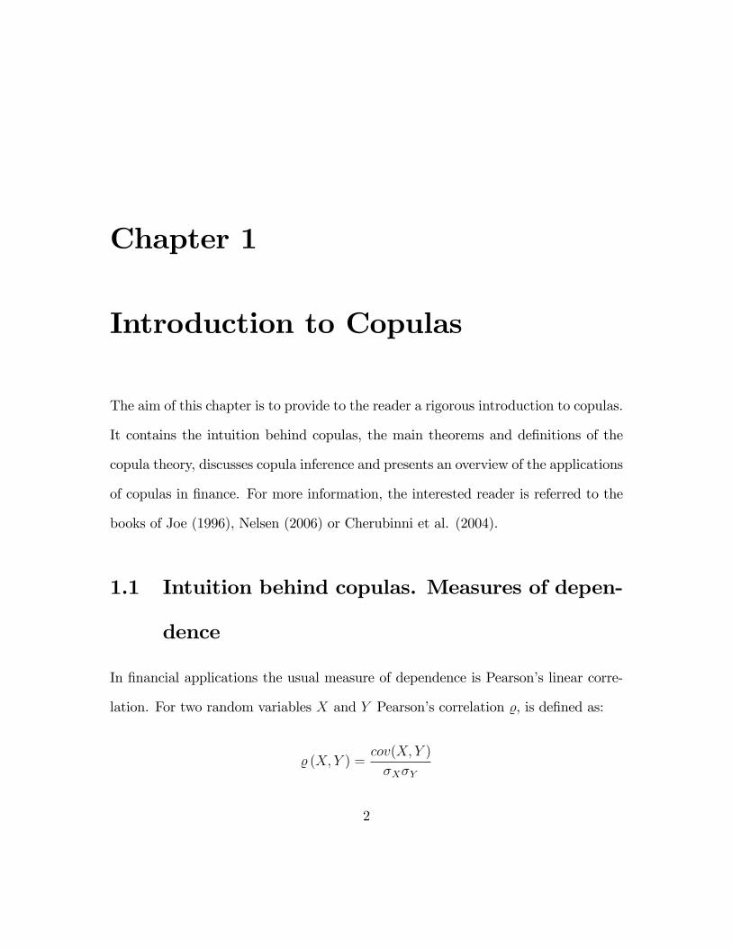
functions f and g. To make this more clear consider the case of two independent
standard normal variables X, Y and the transformation f(x) = exp(x). Figure 1.1
contains the Scatterplots of 100 realizations of (X, Y ) (left panel) and (f(X), f(Y ))
(right panel). The distortion of the dependence structure caused by the nonlinear
transformation is clear.
4 3 2 1 0 1 2 33
2
1
0
1
2
3
4Scatterplot X~N(0,1) & Y~N(0,1), sample rho = 0.1267
X~N(0,1)
Y~N
(0,1
)
0 2 4 6 8 10 12 14 16 18 200
5
10
15
20
25
W = exp(X)
Z =
exp(
Y)
Scatterplot of W and Z, sample rho = 0.0463
Figure 1.1 : Scatterplot of 100 realizations of two independent standard normal variables (left
panel) and of their transformation, created by f(x) = exp(x)
Therefore a measure of dependence more appropriate that the linear correlation
should not depend on X and Y and thus preserve the dependence for both pairs
(X, Y ) and (f(X), g(Y )). The remedy to this invariance problem is to use not the
3
data sample but the ranks associated with the sample. Let sXi and sY i denote the
ranks of observations Xi and Yi (Note: The rank of the observation Xi is the position
of Xi if the sample was set in increasing order, that is the smallest value of Xi would
have rank 1, the second smallest value of Xi would have rank 2, the biggest value of
Xi, in a sample of size n, would have rank n and so on). But since the ranks depend
on the sample size, instead of them the standardized ranks, SXi, SY i are used
SXi =sXin+ 1
, SY i =sY in+ 1
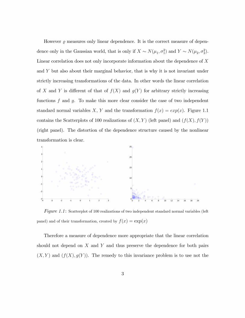
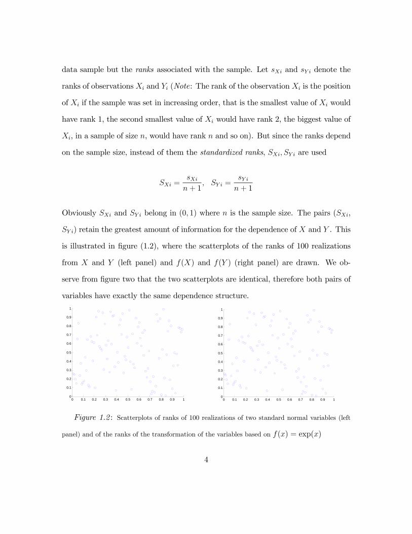
Obviously SXi and SY i belong in (0, 1) where n is the sample size. The pairs (SXi,
SY i) retain the greatest amount of information for the dependence of X and Y . This
is illustrated in figure (1.2), where the scatterplots of the ranks of 100 realizations
from X and Y (left panel) and f(X) and f(Y ) (right panel) are drawn. We ob-
serve from figure two that the two scatterplots are identical, therefore both pairs of
variables have exactly the same dependence structure.
0 0.1 0.2 0.3 0.4 0.5 0.6 0.7 0.8 0.9 10
0.1
0.2
0.3
0.4
0.5
0.6
0.7
0.8
0.9
1scatterplot of ranks of two independend standrad normal variables
0 0.1 0.2 0.3 0.4 0.5 0.6 0.7 0.8 0.9 10
0.1
0.2
0.3
0.4
0.5
0.6
0.7
0.8
0.9
1scatterplot of the rank of two transformed standard normal variable, based on exp(x)
Figure 1.2 : Scatterplots of ranks of 100 realizations of two standard normal variables (left
panel) and of the ranks of the transformation of the variables based on f(x) = exp(x)
4
Nevertheless, the dependence structure of two variables is fully characterized by
the joint distribution F , of the two variables and obviously the distribution function
of the pair (X, Y ) is not the same as the pair (SX , SY ). Hence a question arises:
Is it possible to find (if it exists) a joint distribution, say H, so as to F (X, Y ) =
H (SX , SY )? If such a function exists, it would describe the dependence structure of
X and Y in full, since both SX and SY do not depend on the marginal behavior of
X and Y. The answer to that question was provided by Sklar’s theorem (it will be
presented in the next section). According to it, if X and Y are continuous, such a
function always exists and it is unique. This function is called the copula of X and
Y , which is a Latin word that means link, because it couples the variables to define
their dependence structure.
1.1.1 Rank based measures of dependence
There are many rank based measures of dependence proposed in the statistical lit-
erature. However in this study we will deal only with Srearman’s rho and Kendall’s
tau because they are highly intuitive and they are directly connected to copulas, as
it will become clear in later sections. For more information about other dependence
measures the interested reader is referred to Genest and Verret (2005).
Spearman’s rho
Spearman’s rho is nothing more than Pearson’s linear correlation calculated for
the ranks of the data (Note: To what follows the word ranks will stand for standard-
5
ized ranks, unless otherwise noted)
rn =
n∑i=1
(SXi − SX)(SY i − SY )√n∑i=1
(SXi − SX)2n∑i=1
(SY i − SY )2
where SX = n+1n
n∑i=1
SXi = 12
= n+1n
n∑i=1
SY i = SY .Spearman’s rho has another, more
convenient form
rn =12
n
n∑i=1
SXi · SY i − 3n+ 1
n− 1
Spearman’s rho is theoretically superior than Pearson’s correlation for the follow-
ing reasons
1. It holds that E(rn) = 1 if Y = f(X) for any increasing function f, as opposed
to the linear correlation where E(%n) = 1 if Y = f(X) and f is an increasing
linear function. Analogously E(rn) = −1 if Y = f(X) for any decreasing
function f, as opposed to the linear correlation where E(%n) = −1 if Y = f(X)
and f is an decreasing linear function.
2. Spearman’s rho always exists unlike linear correlation. For example if X or Y
follow student’s t distribution with degree of freedom parameter less than two,
the corresponding variance and therefore the linear correlation does not exist.
3. It is invariant under strictly monotonic transformations; that is rn(X, Y ) =
rn(g(X), g(Y )) unlike linear correlation where %(X, Y ) 6= %(g(X), g(Y )), for
any strictly increasing function g.
6
Kendall’s tau
Kendall’s tau is based on the notion of concordance: Two pairs (Xi, Yi) and
(Xj, Yj) will be called concordant when (Xi, Yi) (Xj, Yj) > 0.If the two pairs are not
concordant they will be called discordant. The sample estimator of Kendall’s tau is
τn =Pn −Qn(
n2
) =4
n (n− 1)Pn − 1
where Pn and Qn are the number of concordant and discordant pairs.τn is a rank
based measure since (Xi, Yi) (Xj, Yj) > 0 if and only if (SXi − SXj)(SY i − SY j) >
0. Kendall’s tau shares all three characteristics of Spearman’s rho, that make it a
superior dependence measure when compared to the linear correlation and further
it is directly linked to a class of copulas named Archimedean copulas, as I will
demonstrate to the next section.
1.2 Definitions and fundamental properties
Definition 1 A copula is a multivariate distribution with uniform margins.
An equivalent, more mathematical definition is the following:
Definition 2 A Copula is a function C : [0, 1]d −→ [0, 1] , that satisfies the following
conditions:
1. For all (u1, u2, ..., ud) in [0, 1]d , if at least one component ui is zero then C(u1, u2, ..., ud) =
0
7
2. For every ui ∈ [0, 1], C (1, ..., 1, ui, ...1) = ui, for i = 1, 2, ..., d
3. For all [u11, u12]×[u21, u22]×...×[ud1, ud2] d - dimensional rectangles in [0, 1]d ,it
holds that ∑...∑
(−1)i1+...+id C (u1i1 , u2i2 , ..., udid) > 0
Copulas allow as to separate the marginal behavior of a multivariate distribution,
from the dependence structure as it was proven by Sklar (1959).
Theorem 3 (Sklar’s theorem) Let F be a d−dimensional distribution function with
univariate margins F1, ..., Fd with domains D1, ..., Dd respectively. Then there exists
a unique function H , defined on D1 ×D2 × ...×Dd, such that:
F (x1, ..., xd) = H (F1 (x1) , ..., Fd (xd)) .
The extension of H to [0, 1]d is a copula C. For such a function C we have:
F (x1, ..., xd) = C (F1 (x1) , ..., Fd (xd)) . (1.1)
If the marginal distributions Fi, i = 1, 2, ..., d are continuous, the function H co-
incides with the copula C, which is then unique. Conversely, for given univariate
distributions functions F1, ..., Fd and a d− dimensional copula C, the function defined
by:
F (x1, ..., xd) = C (F1 (x1) , ..., Fd (xd))
is a d− dimensional distribution function with univariate margins F1, ..., Fd.
8
Remark 4 To everything that follows, distributions will be denoted with capital let-
ters whereas densities will be denoted with small letters. Multivariate functions will
be denoted will bold letters. Further, all marginal distributions are considered con-
tinuous and strictly increasing, unless otherwise mentioned. Finally, the letter u will
be strictly used for uniform variables.
From Sklar’s Theorem we see that a joint distribution is a function of the marginal
distributions and the copula. Since the copula does not depend on the margins
we can say that it represents the dependence between the variables, that is why
a copula is referred to as the dependence structure in the international literature.
Sklar’s theorem provides the tools to construct a joint distribution from its marginal
distributions and a copula but it doesn’t say anything on how the copula distribution
can be constructed, from the corresponding joint distribution. Before doing so we
need the definition of the probability integral transformation.
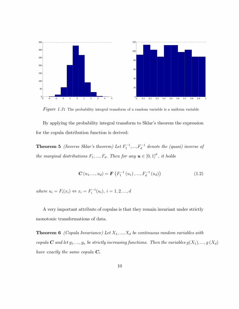
Let X1, ..., Xd be random variables with distributions F1, ..., Fd, respectively. The
probability integral transformation is a function T : Rd −→ [0, 1]d, such that: (x1, ..., xd)T−→
(F1 (x1) , ..., Fd (xd)) . The inverse of the probability integral transformation T−1 :
[0, 1]d −→ Rd is called the quantile transformation and it is defined as: (u1, ..., ud)T−1−→(
F−11 (u1) , ..., F−1
d (ud)). Obviously the probability integral transformation of a ran-
dom variable is a uniform variable, as depicted in figure 1.3, where a histogram of
1000 simulated values from the t5 distribution is plotted (left panel) and its corre-
sponding probability integral transformation.
9
5 4 3 2 1 0 1 2 3 4 50
50
100
150
200
250
300
350histogramm of a t(10) random variable
0 0.1 0.2 0.3 0.4 0.5 0.6 0.7 0.8 0.9 10
20
40
60
80
100
120histogramm of the PIT transform of the t(5) variable
Figure 1.3 : The probability integral transform of a random variable is a uniform variable
By applying the probability integral transform to Sklar’s theorem the expression
for the copula distribution function is derived:
Theorem 5 (Inverse Sklar’s theorem) Let F−11 ,...,F−1
d denote the (quasi) inverse of
the marginal distributions F1, ..., Fd. Then for any u ∈ [0, 1]d , it holds
C (u1, ..., ud) = F(F−1
1 (u1) , ..., F−1d (ud)
)(1.2)
where ui = Fi(xi)⇔ xi = F−1i (ui), i = 1, 2, ..., d
A very important attribute of copulas is that they remain invariant under strictly
monotonic transformations of data.
Theorem 6 (Copula Invariance) Let X1, ..., Xd be continuous random variables with
copulaC and let g1, ..., gn be strictly increasing functions. Then the variables g(X1), ..., g (Xd)
have exactly the same copula C.
10
From equations (1.1) and (1.2) the expression of the corresponding densities can
be derived. By taking derivatives to equation (1.1) we have:
f (x1, ..., xd) =∂dF (x1, ..., xd)
∂x1 · ... · ∂xd=∂dC (F1 (x1) , ..., Fd (xd))
∂x1 · ... · ∂xd=
=∂dC (F1 (x1) , ..., Fd (xd))
∂F1 (x1) · ... · ∂Fd (xd)
d∏i=1
dFi (xi)
dxi=
= c (F1 (x1) , ..., Fd (xd)) ·d∏i=1
fi (xi) (1.3)
and, analogously, equation (1.2) becomes:
c (u1, ..., ud) =f(F−1
1 (u1) , ..., F−1d (ud)
)d∏i=1
fi (F−1(ui))
(1.4)
Equations (1.2) and (1.4) are of extreme importance because they provide a tool
to create the copula density (and therefore the log - likelihood) that describes the
dependence structure of some common multivariate densities.
Example 7 (The Gaussian Copula) The Gaussian Copula describes the dependence
structure of the multivariate Gaussian distribution. Let X be a d−dimensional ran-
dom vector that follows the Gaussian distribution with zero mean and correlation
matrix Σ. Then the random vector U = (Φ (x1) , ...,Φ (xd)) follows the Gaussian
Copula, with distribution and density defined as:
CG (u1, ..., ud) = ΦΣ
(Φ−1 (u1) , ...,Φ−1 (ud)
)
11
and
cG (u1, ..., ud) =φΣ (Φ−1 (u1) , ...,Φ−1 (ud))
d∏i=1
φi (Φ−1(ui))
(1.5)
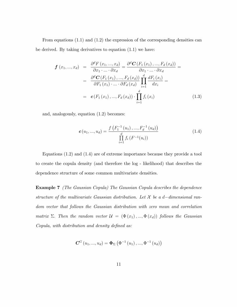
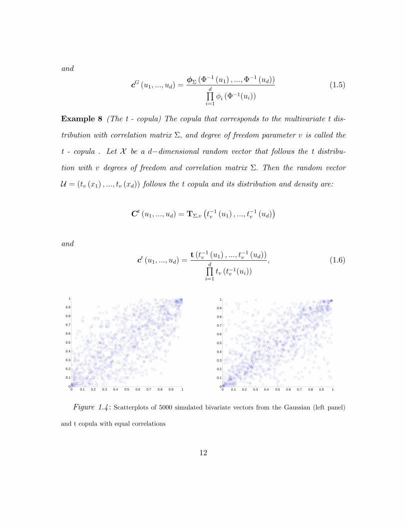
Example 8 (The t - copula) The copula that corresponds to the multivariate t dis-
tribution with correlation matrix Σ, and degree of freedom parameter v is called the
t - copula . Let X be a d−dimensional random vector that follows the t distribu-
tion with v degrees of freedom and correlation matrix Σ. Then the random vector
U = (tv (x1) , ..., tv (xd)) follows the t copula and its distribution and density are:
Ct (u1, ..., ud) = TΣ,v
(t−1v (u1) , ..., t−1
v (ud))
and
ct (u1, ..., ud) =t (t−1
v (u1) , ..., t−1v (ud))
d∏i=1
tv (t−1v (ui))
, (1.6)
0 0.1 0.2 0.3 0.4 0.5 0.6 0.7 0.8 0.9 10
0.1
0.2
0.3
0.4
0.5
0.6
0.7
0.8
0.9
1Scatterplot of simulated values from a Gaussian Copula with rho = .75
0 0.1 0.2 0.3 0.4 0.5 0.6 0.7 0.8 0.9 10
0.1
0.2
0.3
0.4
0.5
0.6
0.7
0.8
0.9
1Scatterplot of simulated values from a t copula with rho = .75 and v = 3
Figure 1.4 : Scatterplots of 5000 simulated bivariate vectors from the Gaussian (left panel)
and t copula with equal correlations
12
The Gaussian and t copula are constructed by applying Sklar’s theorem to the
multivariate Gaussian and multivariate t distribution, respectively. Another way of
constructing copulas is by the use of a copula generator function ψ. The copulas
constructed this way are called Archimedean copulas
Definition 9 (Archimedean Copulas) An Archimedean copula is a function C from
[0, 1]d −→ [0, 1] given by:
C (u1, ..., ud) = ψ[−1]
(d∑i=1
ψ (ui)
)(1.7)
where ψ (the generator function of C) is a continuous, strictly decreasing convex
function from [0, 1] to [0,+∞) such that ψ(1) = 0 and where ψ[−1] denotes the pseudo
- inverse function of ψ :
ψ[−1] (t) =
ψ−1 (t) for 0 6 t < ψ(0)
0 for t > ψ(0)
When ψ (0) = ∞, ψ and C are said to be strict (and ψ[−1] (t) = ψ−1 (t)); when
ψ (0) < ∞ ψ and C are non - strict. Furthermore, C (u1, ..., ud) > 0 on (0, 1]d if
and only if C is strict.
The term Archimedean copulas first appeared in Genest and Mackay (1995). It
arises from the fact that the copulas constructed by the equation (1.7) follow the
Archimedean property (Genest and Favre, 2007), which states that if u and v are
real numbers in (0, 1) there exists an integer n such that un < v. Given a copula
C, the "C − multiplication" is defined by u v = C (u, v) .Then un is defined
13
recursively by u2 = u u and un = un−1 u [Note: Non Archimedean copulas also
have this property, as long as C(u, u) < u for u in (0, 1).]
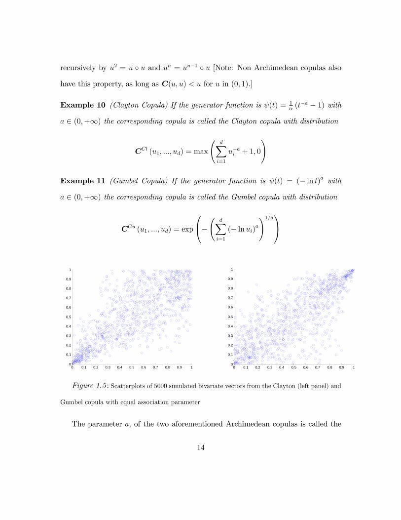
Example 10 (Clayton Copula) If the generator function is ψ(t) = 1α
(t−a − 1) with
a ∈ (0,+∞) the corresponding copula is called the Clayton copula with distribution
CCl (u1, ..., ud) = max
(d∑i=1
u−ai + 1, 0
)
Example 11 (Gumbel Copula) If the generator function is ψ(t) = (− ln t)a with
a ∈ (0,+∞) the corresponding copula is called the Gumbel copula with distribution
CGu (u1, ..., ud) = exp
−( d∑i=1
(− lnui)a
)1/a
0 0.1 0.2 0.3 0.4 0.5 0.6 0.7 0.8 0.9 10
0.1
0.2
0.3
0.4
0.5
0.6
0.7
0.8
0.9
1Scatterplot of random values simulated from a Clayton Copula with a = 2.35
0 0.1 0.2 0.3 0.4 0.5 0.6 0.7 0.8 0.9 10
0.1
0.2
0.3
0.4
0.5
0.6
0.7
0.8
0.9
1Scatterplot of random values simulated from a Gumbel copula with a = 2.17
Figure 1.5 : Scatterplots of 5000 simulated bivariate vectors from the Clayton (left panel) and
Gumbel copula with equal association parameter
The parameter a, of the two aforementioned Archimedean copulas is called the
14
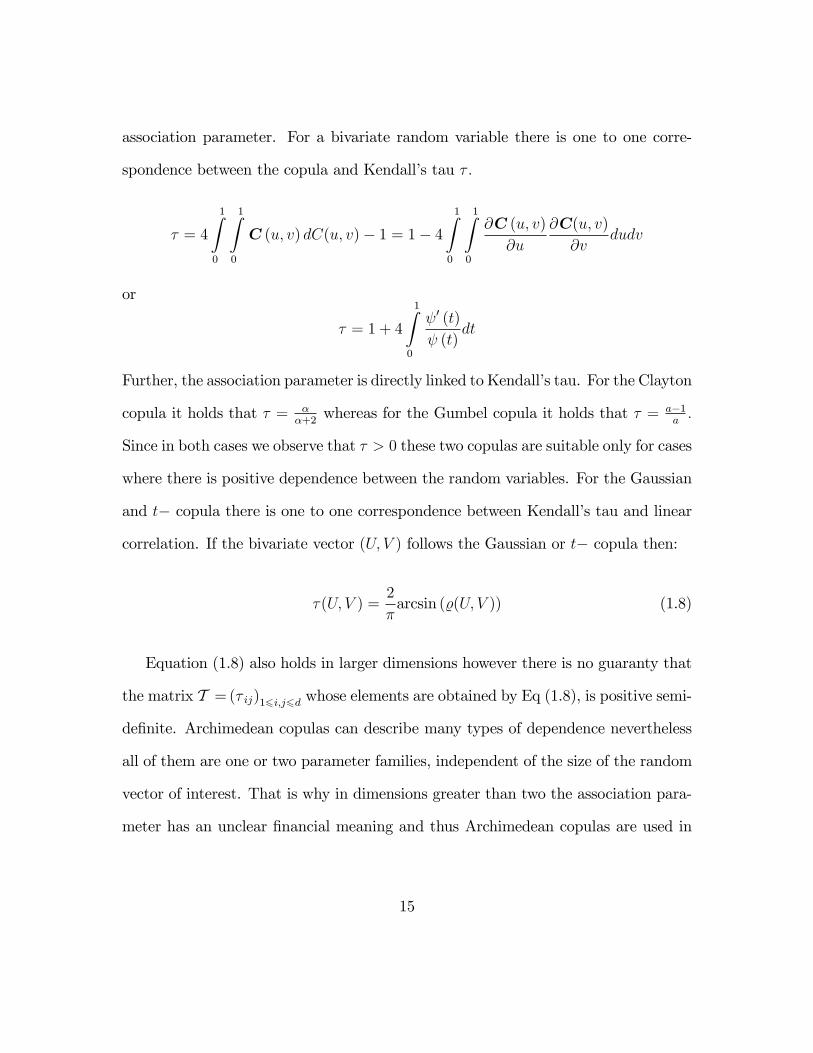
association parameter. For a bivariate random variable there is one to one corre-
spondence between the copula and Kendall’s tau τ .
τ = 4
1∫0
1∫0
C (u, v) dC(u, v)− 1 = 1− 4
1∫0
1∫0
∂C (u, v)
∂u
∂C(u, v)
∂vdudv
or
τ = 1 + 4
1∫0
ψ′ (t)
ψ (t)dt
Further, the association parameter is directly linked to Kendall’s tau. For the Clayton
copula it holds that τ = αα+2
whereas for the Gumbel copula it holds that τ = a−1a.
Since in both cases we observe that τ > 0 these two copulas are suitable only for cases
where there is positive dependence between the random variables. For the Gaussian
and t− copula there is one to one correspondence between Kendall’s tau and linear
correlation. If the bivariate vector (U, V ) follows the Gaussian or t− copula then:
τ(U, V ) =2
πarcsin (%(U, V )) (1.8)
Equation (1.8) also holds in larger dimensions however there is no guaranty that
the matrix T = (τ ij)16i,j6d whose elements are obtained by Eq (1.8), is positive semi-
definite. Archimedean copulas can describe many types of dependence nevertheless
all of them are one or two parameter families, independent of the size of the random
vector of interest. That is why in dimensions greater than two the association para-
meter has an unclear financial meaning and thus Archimedean copulas are used in
15
financial applications strictly for bivariate problems. Therefore in what follows we
will consider only bivariate Archimedean copulas.
1.3 Tail dependence
In applications related to risk management, the tails of the returns distribution
are of extreme importance, since the risk metric proposed by the Bassel accord for
financial institutions (Value at Risk) is related to the quantile function of the returns.
Analogously, in the multivariate setting, the accurate calculation of the probability
of a joint extreme event (stock market crush or simultaneous default of the majority
of loans, in a loan portfolio) is essential. A measure of this probability is the tail
dependence. Let X and Y be two random variables with distributions FX and FY .
The limit (if it exists) of the conditional probability that Y is greater than the 100th
- percentile of FY , given that X is greater than the 100th percentile of FX is called
upper tail dependence and is denoted as λU
λU = limu−→1−
Pr[Y > F−1
Y (u)|X > F−1X (u)
]Similarly the limit of the conditional probability that Y is less than or equal to the
100th - percentile of FY , given that X is less than or equal to the 100th percentile
of FX is called lower tail dependence and is denoted as λL
λL = limu−→0+
Pr[Y 6 F−1
Y (u)|X 6 F−1X (u)
]
16
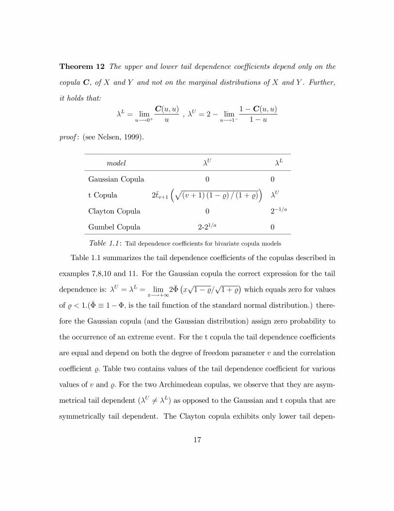
Theorem 12 The upper and lower tail dependence coeffi cients depend only on the
copula C, of X and Y and not on the marginal distributions of X and Y . Further,
it holds that:
λL = limu−→0+
C(u, u)
u, λU = 2− lim
u−→1−
1−C(u, u)
1− u
proof : (see Nelsen, 1999).
model λU λL
Gaussian Copula 0 0
t Copula 2tv+1
(√(v + 1) (1− %) / (1 + %)
)λU
Clayton Copula 0 2−1/a
Gumbel Copula 2-21/a 0
Table 1.1 : Tail dependence coeffi cients for bivariate copula models
Table 1.1 summarizes the tail dependence coeffi cients of the copulas described in
examples 7,8,10 and 11. For the Gaussian copula the correct expression for the tail
dependence is: λU = λL = limx−→+∞
2Φ(x√
1− %/√
1 + %)which equals zero for values
of % < 1.(Φ ≡ 1−Φ, is the tail function of the standard normal distribution.) there-
fore the Gaussian copula (and the Gaussian distribution) assign zero probability to
the occurrence of an extreme event. For the t copula the tail dependence coeffi cients
are equal and depend on both the degree of freedom parameter v and the correlation
coeffi cient %. Table two contains values of the tail dependence coeffi cient for various
values of v and %. For the two Archimedean copulas, we observe that they are asym-
metrical tail dependent (λU 6= λL) as opposed to the Gaussian and t copula that are
symmetrically tail dependent. The Clayton copula exhibits only lower tail depen-
17
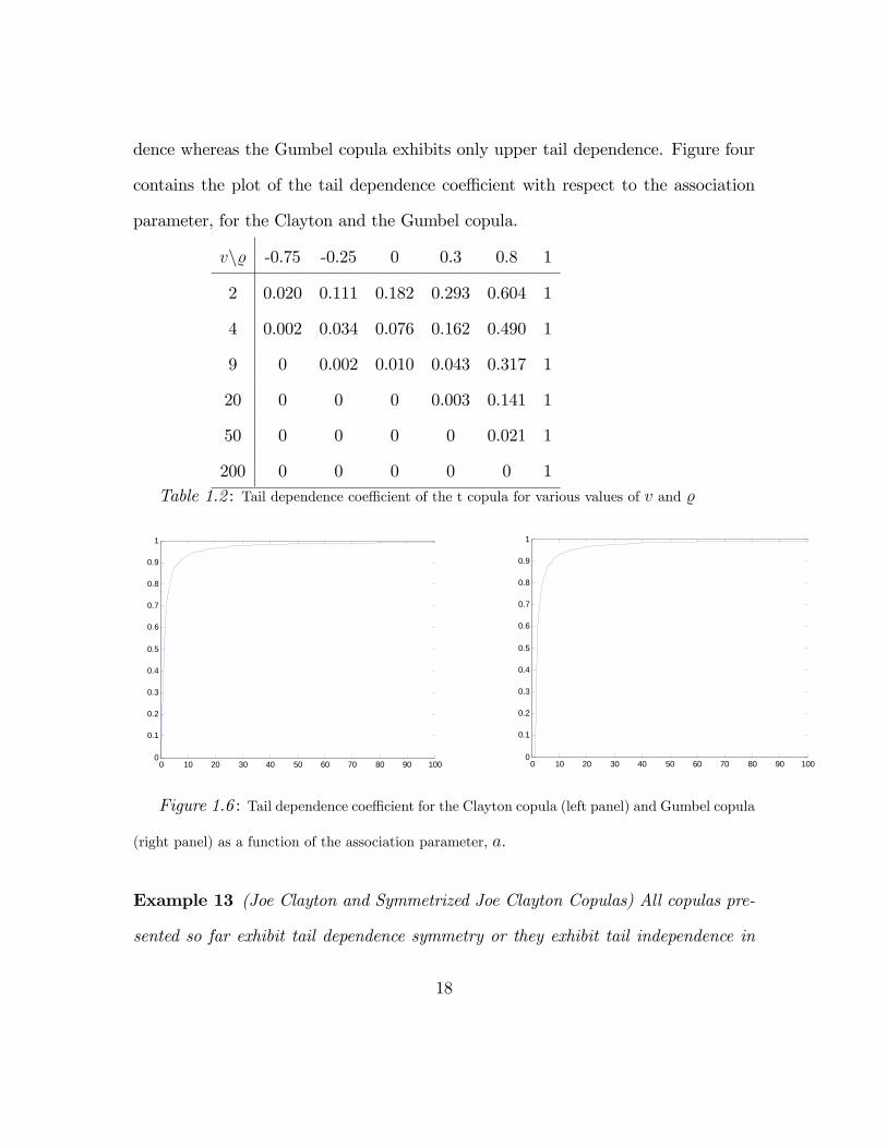
dence whereas the Gumbel copula exhibits only upper tail dependence. Figure four
contains the plot of the tail dependence coeffi cient with respect to the association
parameter, for the Clayton and the Gumbel copula.
v\% -0.75 -0.25 0 0.3 0.8 1
2 0.020 0.111 0.182 0.293 0.604 1
4 0.002 0.034 0.076 0.162 0.490 1
9 0 0.002 0.010 0.043 0.317 1
20 0 0 0 0.003 0.141 1
50 0 0 0 0 0.021 1
200 0 0 0 0 0 1Table 1.2 : Tail dependence coeffi cient of the t copula for various values of v and %
0 10 20 30 40 50 60 70 80 90 1000
0.1
0.2
0.3
0.4
0.5
0.6
0.7
0.8
0.9
1Kendall's tau of the Clayton Copula for various values of a
0 10 20 30 40 50 60 70 80 90 1000
0.1
0.2
0.3
0.4
0.5
0.6
0.7
0.8
0.9
1Kendall's tau of the Gumbel copula for various values of a
Figure 1.6 : Tail dependence coeffi cient for the Clayton copula (left panel) and Gumbel copula
(right panel) as a function of the association parameter, a.
Example 13 (Joe Clayton and Symmetrized Joe Clayton Copulas) All copulas pre-
sented so far exhibit tail dependence symmetry or they exhibit tail independence in
18
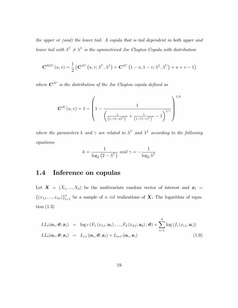
the upper or (and) the lower tail. A copula that is tail dependent in both upper and
lower tail with λU 6= λL is the symmetrized Joe Clayton Copula with distribution
CSGC (u, v) =1
2
(CJC
(u, v;λU , λL
)+CJC
(1− u, 1− v;λL, λU
)+ u+ v − 1
)where CJC is the distribution of the Joe Clayton copula defined as
CJC(u, v) = 1−
1− 1(1
(1−(1−u)k)γ + 1
(1−(1−v)k)γ − 1
)1/γ
1/k
where the parameters k and γ are related to λU and λL according to the following
equations
k =1
log2
(2− λU
) and γ = − 1
log2 λL
1.4 Inference on copulas
Let X = (X1, ..., Xd) be the multivariate random vector of interest and xt =
(x1,t, ..., xd,t)nt=1 be a sample of n iid realizations of X. The logarithm of equa-
tion (1.3)
LLt(αi,ϑ;xt) = log c (F1 (x1,t;a1) , ..., Fd (xd,t;ad) ;ϑ) +
d∑i=1
log (fi (xi,t;ai))
LLt(αi,ϑ;xt) = Lc,t (αi,ϑ;xt) + Lm,t (αi,xt) (1.9)
19
is the log - likelihood function for the t − th observation of a copula based model,
where αi is the vector of parameters of the i − th margin and ϑ is the vector of
copula parameters. To estimate the parameters vector φ = (a′1, ...,a′d,ϑ
′)′ three
methods have been proposed in the statistical literature, maximum likelihood (MLE),
Inference function for margins (IFM) and the pseudo likelihood method (PML).
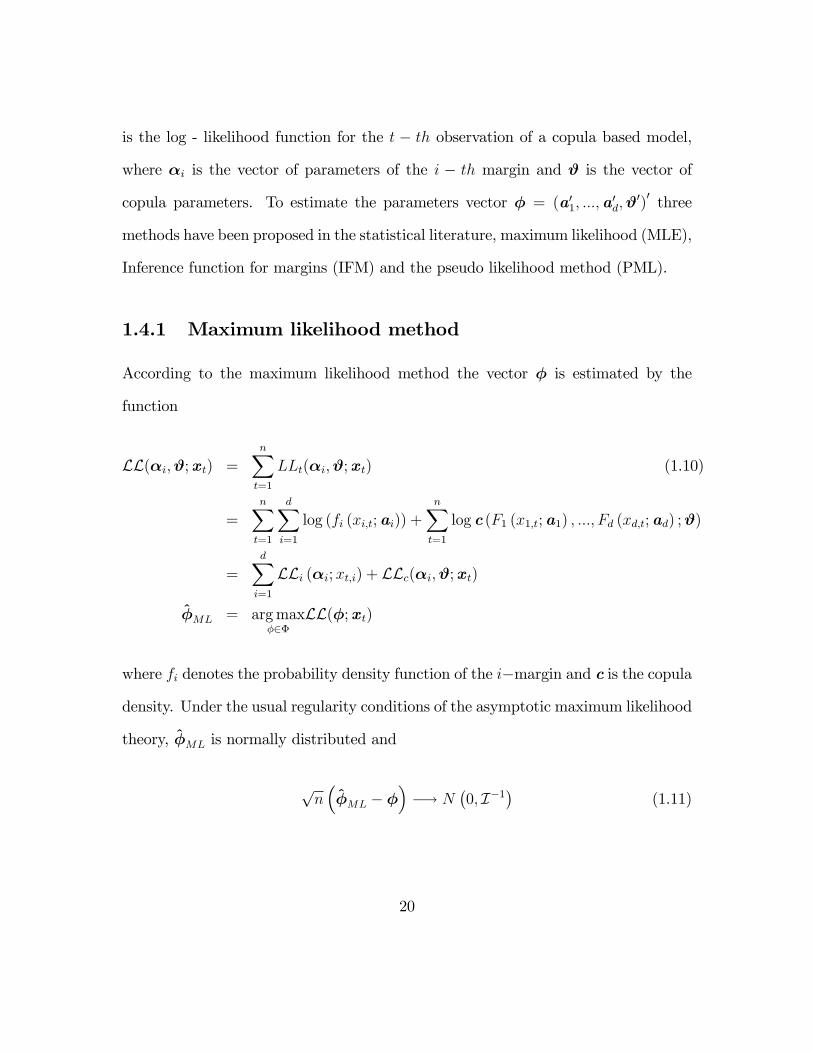
1.4.1 Maximum likelihood method
According to the maximum likelihood method the vector φ is estimated by the
function
LL(αi,ϑ;xt) =n∑t=1
LLt(αi,ϑ;xt) (1.10)
=n∑t=1
d∑i=1
log (fi (xi,t;ai)) +n∑t=1
log c (F1 (x1,t;a1) , ..., Fd (xd,t;ad) ;ϑ)
=d∑i=1
LLi (αi;xt,i) + LLc(αi,ϑ;xt)
φML = arg maxφ∈Φ
LL(φ;xt)
where fi denotes the probability density function of the i−margin and c is the copula
density. Under the usual regularity conditions of the asymptotic maximum likelihood
theory, φML is normally distributed and
√n(φML − φ
)−→ N
(0, I−1
)(1.11)
20
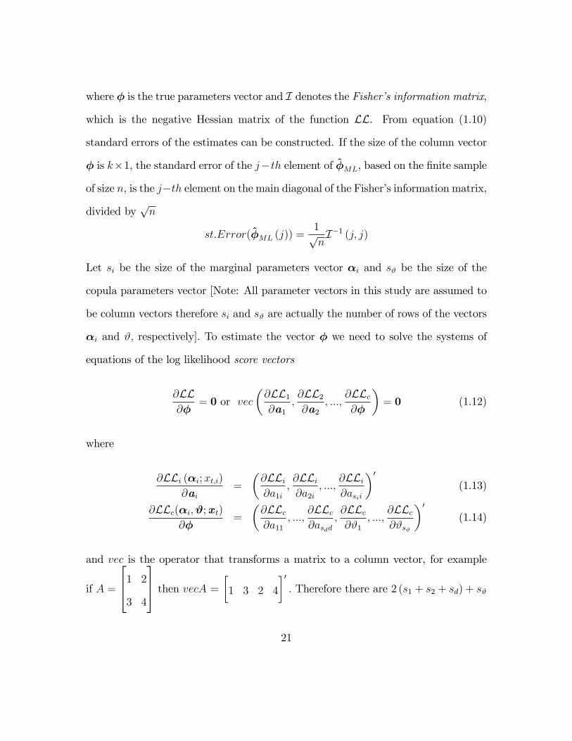
where φ is the true parameters vector and I denotes the Fisher’s information matrix,
which is the negative Hessian matrix of the function LL. From equation (1.10)
standard errors of the estimates can be constructed. If the size of the column vector
φ is k×1, the standard error of the j−th element of φML, based on the finite sample
of size n, is the j−th element on the main diagonal of the Fisher’s information matrix,
divided by√n
st.Error(φML (j)) =1√nI−1 (j, j)
Let si be the size of the marginal parameters vector αi and sϑ be the size of the
copula parameters vector [Note: All parameter vectors in this study are assumed to
be column vectors therefore si and sϑ are actually the number of rows of the vectors
αi and ϑ, respectively]. To estimate the vector φ we need to solve the systems of
equations of the log likelihood score vectors
∂LL∂φ
= 0 or vec
(∂LL1
∂a1
,∂LL2
∂a2
, ...,∂LLc∂φ
)= 0 (1.12)
where
∂LLi (αi;xt,i)∂ai
=
(∂LLi∂a1i
,∂LLi∂a2i
, ...,∂LLi∂asii
)′(1.13)
∂LLc(αi,ϑ;xt)
∂φ=
(∂LLc∂a11
, ...,∂LLc∂asdd
,∂LLc∂ϑ1
, ...,∂LLc∂ϑsϑ
)′(1.14)
and vec is the operator that transforms a matrix to a column vector, for example
if A =
1 2
3 4
then vecA = [1 3 2 4
]′. Therefore there are 2 (s1 + s2 + sd) + sϑ
21
equations based on the first derivatives of the log likelihood function that need to
be solved. It is obvious that the number of equations grows with d, making very
diffi cult to estimate such models in large dimensions. Further, the calculations of the
analytical scores of the log likelihood can be very tedious, that is why solving the
equations defined in (1.12) is a method to estimate φ that is never used in practice.
Instead numerical methods are usually employed. The term "numerical methods"
covers all methods where the optimum vector is not obtained by solving systems of
equations but by an iterative process based on numerical approximations of the log
likelihood gradient vector and Hessian matrix. A hybrid method of the two main-
tains the iterative scheme of the numerical methods but uses analytical expressions
for the gradient vector and/or the Hessian matrix of the log likelihood. The analyt-
ical derivatives based method is more effi cient when compared to numerically based
derivatives method, in both accuracy and speed of convergence, as it was advocated
in Hafner and Herwartz (2007) or in Diamantopoulos and Vrontos (2010), in a simi-
lar context. In what follows, when we refer to numerical optimization we mean the
iterative process that uses numerical approximations of the gradient and Hessian,
as opposed to the analytical optimization method where again an iterative process
is employed but with analytical expressions for the log likelihood gradient and the
Hessian. The iterative process that is usually employed is the so called BFGS al-
gorithm (Goldfarb (1970) and Shanno (1970)), according to which the parameters
vector φpobtained after p− iterations of the algorithm, equals
φp
= φp−1 − λH−1∂LL
∂φ(1.15)
22

where λ is a scalar that controls the step size, H is some approximation of the
Hessian, computed at φp−1and defines the direction of the search. In case where
the actual Hessian (numerical or analytical) is used, the BFGS method is known as
Newton - Raphson (NR) method, while if H is approximated by the outer product
of gradients
H =
(∂LL∂φ
)′∂LL∂φ
the method is known as BHHH method, from Berndt, Hall, Hall and Hausman
(1970). For more information on optimization methods the interested reader is re-
ferred to Fletcher and Roger (1987) or Avriel and Mordecai (2003). Nevertheless,
numerical methods (we are not aware of any attempt to estimate copulas with ana-
lytical methods, except of Liu and Luger (2009) who used analytical derivatives to
test a novel estimation method called maximization by parts. However they used
the analytical method to the simplest case possible, Gaussian copula with Gaussian
margins.) speed and accuracy depend heavily on the size of the parameters vector.
Therefore in empirical applications the maximum likelihood method is rarely used.
Instead, two step methods, like the IFM or the PML methods are employed.
1.4.2 Inference functions for margins (IFM)
The IFM method was proposed by Joe (1996) and is a fully parametric method
that consists of two steps. Its basic idea is instead of optimizing the log likelihood
function (LL, in equation (1.10)), to optimize LLi, i = 1, 2, ..d independently from
each other, in order to obtain estimates for the marginal parameters vectors αi at
23
the first step and at the second step the function LLc is optimized, conditioned upon
the results from the first step. Therefore the score vector of the first step for the i−
margin is
∂LLi (αi;xt,i)∂ai
=
(∂LLi∂a1i
,∂LLi∂a2i
, ...,∂LLi∂asii
)′i = 1, 2, ..., d.
Note that the above expression is identical to equation(1.13) thus the marginal esti-
mates of both methods are identical. At the second step the conditional score vector
equations obtained by the copula log likelihood, are used to estimate the copula
parameters∂LLc(ϑ;αi,xt)
∂ϑ=
(∂LLc∂ϑ1
, ...,∂LLc∂ϑsϑ
)′(1.16)
In other words, IFM method assumes working independence between the marginal
parameters and the copula log - likelihood. The procedure that is used to estimate
the parameters, with the IFM, is similar to that of the MLE method. One can
solve the systems of equations defined by the log likelihood scores or use an iterative
algorithm, as it is always done in practice. Let gk,n be the score vectors defined in
(1.13) and (1.16)
gk,n = vec
(∂LLi (αi;xt,i)
∂ai,∂LLc(ϑ;αi,xt)
∂ϑ
)
Joe proved that the variance - covariance matrix Vn, of the parameters vector φ,
based on the finite sample of size n, is given by the Godambe Information matrix,
24
defined as
Vn = H−1n JnH
−1n
whereHn =∂gk,n∂φ′ =
∂2LLi∂ai∂a′j
0
0 ∂2LLc∂ϑ∂ϑ′
and Jn = gk,n ·g′k,n.Van der Vaart (1998) argued
that instead of the Godambe information matrix , the variance covariance matrix
of the parameters can be obtained by applying one step of the Newton - Raphson
algorithm to the full likelihood, using the IFM estimators. An alternative method to
calculate the variance covariance matrix under the IFM framework is the jackknife
method (Dias, 2004).
Proposition 14 (Joe, 1996, page 302) Let φ(−t)
, t = 1, 2, ..., n be the IFM estimate
of φ obtained from the observed sample, with the t - th observation excluded. The
jackknife estimate of Vn is
Vn = nn∑t=1
(φ
(−t) − φ)(φ
(−t) − φ)′
Further, if h is a real valued function, the standard errors of h(φ)are given by
(n∑t=1
(h(φ
(−t))− h(φ)))1/2
.
1.4.3 The pseudo likelihood method
As it was pointed out in subsection 1.1 the copula of a d− dimensional random vector
X is the joint distribution of the ranks associated with X. In both MLE and IFM
25
methods the ranks of X are obtained for the probability integral transformation of
X, that is by assuming a marginal distribution Fi for Xi and calculating the ranks
of Xi, for a sample of size n by Fi (xi,t) , i = 1, .., d t = 1, ..., n. Therefore the correct
choice of the marginal distribution Fi is crucial for the accuracy of the method, as
noted for example in Kim et al. (2007). To avoid this potential pitfall, Genest and
Rivest (1995) proposed to calculate the ranks of the data not with the parametric
probability integral transformation but with the non - parametric empirical CDF
function
Fn (x) =1
n+ 1
n∑j=1
Iy∈R,y6x (xij)
Thus, according to the pseudo likelihood method, the n observed d− dimensional
vectors xi = (x1i, ..., xdi)ni=1 are transformed to ranks
(Fn (x1i) , ..., Fn (xdi))
and the copula parameters are estimated by optimizing the corresponding copula log
likelihood
LLc(ϑ;xt) =n∑t=1
log c (Fn (x1,t) , ..., Fd (xd,t) ;ϑ) (1.17)
Genest and Rivest proved the asymptotic normality of the parameters vector ϑPL
obtained by optimizing Eq (1.17).
ϑPL ∼ N(ϑ,v2
n)
26
A consistent estimator of the variance - covariance matrix of ϑPL is
v2n
n=
σ2n
nβ2n
where
σ2n =
1
n
n∑i=1
(Mi − M
)2
and
β2n =
1
n
n∑i=1
(Ni − N
)2
are sample variances computed from two sets of pseudo - observations. These pseudo
observations are computed from a procedure described in Genest and Favre (2007)
for a bivariate data set, as follows:
• Step one: Relabel the original data (X1, Y1), ..., (Xn, Yn), so as to X1 < .... <
Xn
• Step two: Write LLc(ϑ;xt) as L (ϑ,u1, u2) and calculate the derivatives of
eq(1.17) with respect to ϑ, u1 = Fn (x1,t) and u2 = Fn (x2,t) , denoted as Lϑ,
Lu1 and Lu2 , respectively.
• Step three: For i ∈ 1, 2, ..., n, set
Ni = Lϑ
(ϑPL;
i
n+ 1, SY i
)
27
• Step four: For i ∈ 1, 2, ..., n, define
Mi = Ni −1
n
n∑j=1
Lϑ
(ϑPL;
j
n+ 1, SY j
)Lu1
(ϑPL;
j
n+ 1, SY j
)− 1
n
∑SY j>SY i
Lϑ
(ϑPL;
j
n+ 1, SY j
)Lu1
(ϑPL;
j
n+ 1, SY j
)
1.5 Goodness of fit tests for copulas
Let U = (U1, ..., Ud) be a random vector with uniform [0, 1] margins and suppose
we have fitted a copula Cϑn to U , based on a finite sample ut = (u1,t, ..., ud,t)nt=1
of U . A natural question that arises is how good is the fit of Cϑn to the data. To
answer this section we will describe three goodness of fit tests for copulas; a graphical
inspection method, applicable only in the bivariate case, a test for goodness of fit
for the Gaussian and t copula, based on the squared radius of the corresponding
joint distribution, that was developed by Kole et al. (2007) and a test suitable for
Archimedean copulas that is based on the bivariate probability integral transform of
the Archimedean copula, which was originally developed by Wang and Wells (2000)
and generalized by Genest et al. (2006). For a more comprehensive presentation
of goodness of fit tests for copula based models the interested reader is referred to
Genest et al. (2009) who provides a review and a comparison of the various test used
in the copula context.
28
1.5.1 Graphical inspection method
4 3 2 1 0 1 2 3 45
4
3
2
1
0
1
2
3
4scatterplot of two standard normal r.v's with rho = 0.75
0 0.1 0.2 0.3 0.4 0.5 0.6 0.7 0.8 0.9 10
0.1
0.2
0.3
0.4
0.5
0.6
0.7
0.8
0.9
1scatterplot of the ranks of two gaussian r.v's with rho = 0.75
0 0.1 0.2 0.3 0.4 0.5 0.6 0.7 0.8 0.9 10
0.1
0.2
0.3
0.4
0.5
0.6
0.7
0.8
0.9
1scatterplot of a simulated gaussian copula with rho = 0.75
0 0.1 0.2 0.3 0.4 0.5 0.6 0.7 0.8 0.9 10
0.1
0.2
0.3
0.4
0.5
0.6
0.7
0.8
0.9
1scatterplot of 1000 simulated random number from a t copula with rho = 0.75 and dof = 3
0 0.1 0.2 0.3 0.4 0.5 0.6 0.7 0.8 0.9 10
0.1
0.2
0.3
0.4
0.5
0.6
0.7
0.8
0.9
1scatterplot of 1000 simulated random numbers from Clayton copula with a = 2.35
0 0.1 0.2 0.3 0.4 0.5 0.6 0.7 0.8 0.9 10
0.1
0.2
0.3
0.4
0.5
0.6
0.7
0.8
0.9
1scatterplot of 1000 simulated random numbers from a Gumbel copula with a = 2.17
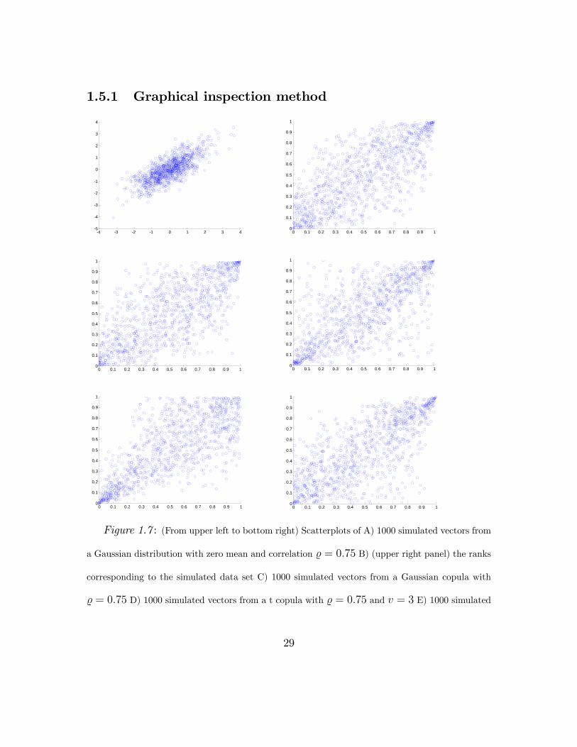
Figure 1.7 : (From upper left to bottom right) Scatterplots of A) 1000 simulated vectors from
a Gaussian distribution with zero mean and correlation % = 0.75 B) (upper right panel) the ranks
corresponding to the simulated data set C) 1000 simulated vectors from a Gaussian copula with
% = 0.75 D) 1000 simulated vectors from a t copula with % = 0.75 and v = 3 E) 1000 simulated
29
vectors from a Clayton copula with a = 2.35 and F) 1000 simulated vectors from a Gumbel copula
with a = 2.17
Let xt = (x1,t, x2,t)nt=1 and ut = (u1,t, u2,t)nt=1 be a sample of the initial ran-
dom vector X and its corresponding ranks, calculated by the probability integral
transform or by the empirical CDF function. The graphical inspection method com-
pares the scatterplots of ut and ut, where ut is a sample of size n, simulated by the
copula model assumed for ut. The copula whose simulated values have scatterplot
that best resembles the scatterplot of ut is the copula with the best fit. In figure
(1.7) the graphical inspection method is illustrated. At the top left panel there is
the scatterplot of 1000 bivariate vectors drawn from a multivariate Gaussian distrib-
ution with correlation coeffi cient % = 0.75 and at the top right panel the scatterplot
of the ranks of the simulated data set is drawn. The other four scatterplots of fig-
ure seven are scatterplots from a) A Gaussian copula with % = 0.75, b) a t copula
with % = 0.75 and degree of freedom parameter v = 3, c) A Clayton copula with
association parameter a = 2.35 and d) A Gumbel copula with association parameter
a = 2.17 (Note: the values of α, for the Clayton and Gumbel copula were chosen to
resemble the case of % = 0.75). It is clear that the scatterplot that best resembles
the one of the ranks (upper right) is the middle left that correspond to the Gaussian
copula. The shortcomings of the graphical inspection are obvious; it can be used
only for bivariate data sets and it does not quantify the goodness of fit with a valid
statistical test but only visualizes the dependence. Further, since this method is
based on simulations from a given parametric copula, it depends on whether the
30
inverse copula distribution exists in closed form
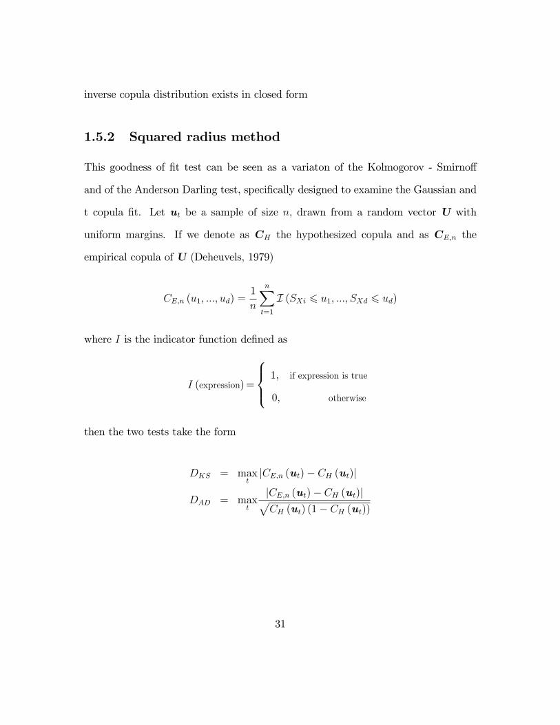
1.5.2 Squared radius method
This goodness of fit test can be seen as a variaton of the Kolmogorov - Smirnoff
and of the Anderson Darling test, specifically designed to examine the Gaussian and
t copula fit. Let ut be a sample of size n, drawn from a random vector U with
uniform margins. If we denote as CH the hypothesized copula and as CE,n the
empirical copula of U (Deheuvels, 1979)
CE,n (u1, ..., ud) =1
n
n∑t=1
I (SXi 6 u1, ..., SXd 6 ud)
where I is the indicator function defined as
I (expression) =
1, if expression is true
0, otherwise
then the two tests take the form
DKS = maxt|CE,n (ut)− CH (ut)|
DAD = maxt
|CE,n (ut)− CH (ut)|√CH (ut) (1− CH (ut))
31
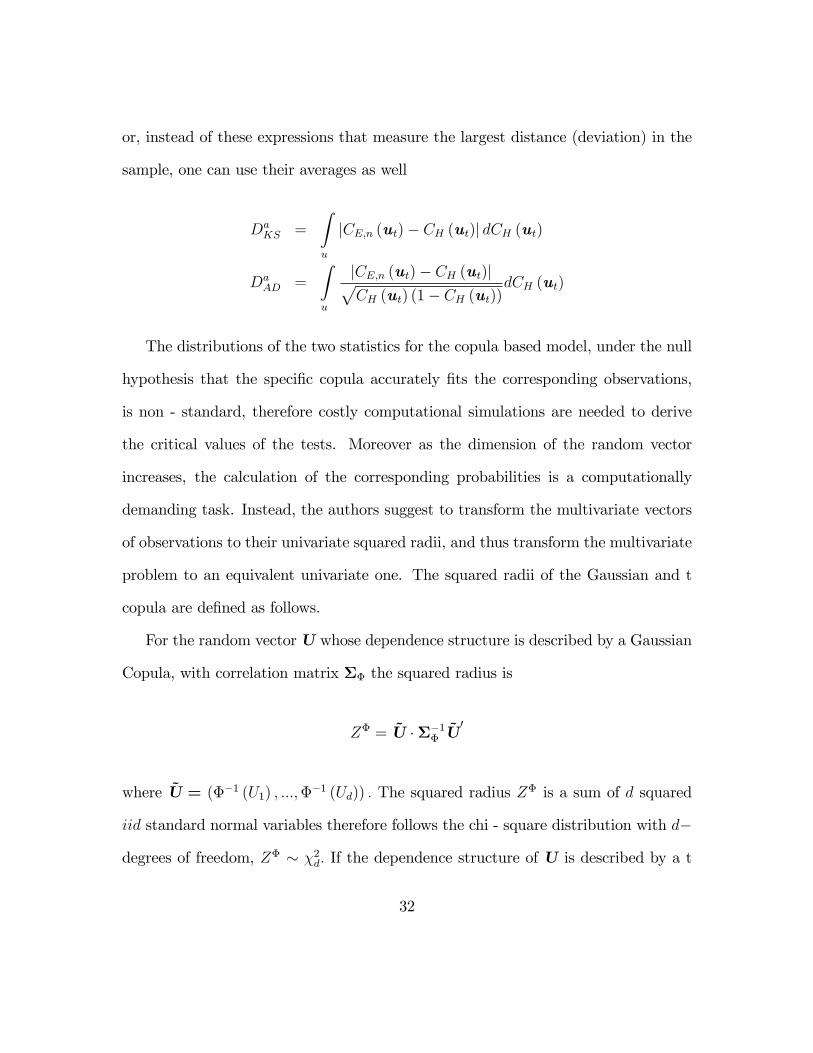
or, instead of these expressions that measure the largest distance (deviation) in the
sample, one can use their averages as well
DaKS =
∫u
|CE,n (ut)− CH (ut)| dCH (ut)
DaAD =
∫u
|CE,n (ut)− CH (ut)|√CH (ut) (1− CH (ut))
dCH (ut)
The distributions of the two statistics for the copula based model, under the null
hypothesis that the specific copula accurately fits the corresponding observations,
is non - standard, therefore costly computational simulations are needed to derive
the critical values of the tests. Moreover as the dimension of the random vector
increases, the calculation of the corresponding probabilities is a computationally
demanding task. Instead, the authors suggest to transform the multivariate vectors
of observations to their univariate squared radii, and thus transform the multivariate
problem to an equivalent univariate one. The squared radii of the Gaussian and t
copula are defined as follows.
For the random vector U whose dependence structure is described by a Gaussian
Copula, with correlation matrix ΣΦ the squared radius is
ZΦ = U ·Σ−1Φ U
′
where U = (Φ−1 (U1) , ...,Φ−1 (Ud)) . The squared radius ZΦ is a sum of d squared
iid standard normal variables therefore follows the chi - square distribution with d−
degrees of freedom, ZΦ ∼ χ2d. If the dependence structure of U is described by a t
32
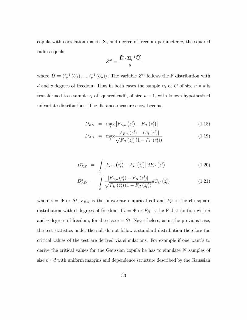
copula with correlation matrix Σt and degree of freedom parameter v, the squared
radius equals
Zst =U ·Σ−1
t U′
d
where U = (t−1v (U1) , ..., t−1
v (Ud)) . The variable Zst follows the F distribution with
d and v degrees of freedom. Thus in both cases the sample ut of U of size n× d is
transformed to a sample zt of squared radii, of size n× 1, with known hypothesized
univariate distributions. The distance measures now become
DKS = maxt
∣∣FE,n (zit)− FH (zit)∣∣ (1.18)
DAD = maxt
|FE,n (zit)− CH (zit)|√FH (zit) (1− FH (zit))
(1.19)
DaKS =
∫z
∣∣FE,n (zit)− FH (zit)∣∣ dFH (zit) (1.20)
DaAD =
∫z
|FE,n (zit)− FH (zit)|√FH (zit) (1− FH (zit))
dCH(zit)
(1.21)
where i = Φ or St, FE,n is the univariate empirical cdf and FH is the chi square
distribution with d degrees of freedom if i = Φ or FH is the F distribution with d
and v degrees of freedom, for the case i = St. Nevertheless, as in the previous case,
the test statistics under the null do not follow a standard distribution therefore the
critical values of the test are derived via simulations. For example if one want’s to
derive the critical values for the Gaussian copula he has to simulate N samples of
size n×d with uniform margins and dependence structure described by the Gaussian
33
copula, transform each of the N samples to their corresponding squared radii, and
calculate the distances defined in equations (1.18) to (1.21), N times. The critical
values of the test are the empirical quantiles of the N simulated values of the distance
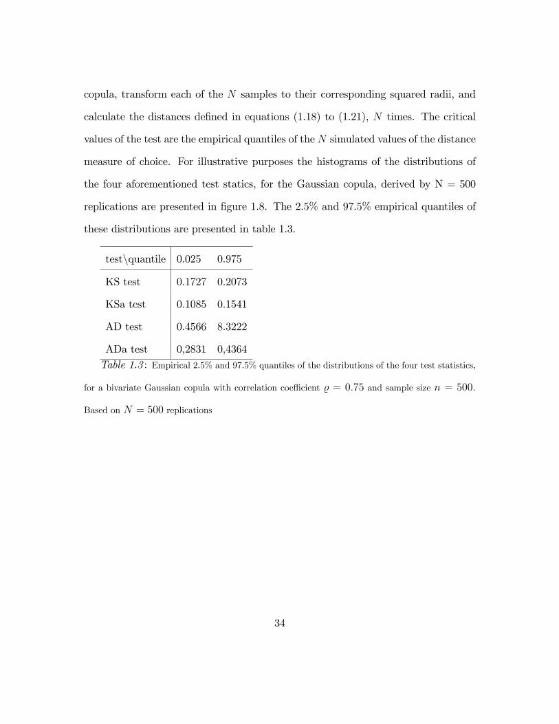
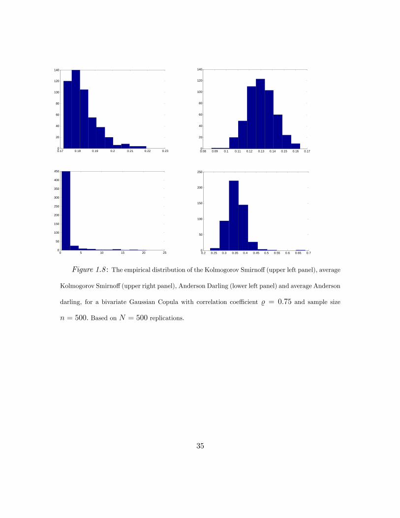
measure of choice. For illustrative purposes the histograms of the distributions of
the four aforementioned test statics, for the Gaussian copula, derived by N = 500
replications are presented in figure 1.8. The 2.5% and 97.5% empirical quantiles of
these distributions are presented in table 1.3.
test\quantile 0.025 0.975
KS test 0.1727 0.2073
KSa test 0.1085 0.1541
AD test 0.4566 8.3222
ADa test 0,2831 0,4364Table 1.3 : Empirical 2.5% and 97.5% quantiles of the distributions of the four test statistics,
for a bivariate Gaussian copula with correlation coeffi cient % = 0.75 and sample size n = 500.
Based on N = 500 replications
34
0.17 0.18 0.19 0.2 0.21 0.22 0.230
20
40
60
80
100
120
140KS test statistic distribution, based on N = 500 replications
0.08 0.09 0.1 0.11 0.12 0.13 0.14 0.15 0.16 0.170
20
40
60
80
100
120
140KSa test statistic distribution, based on N = 500 replications
0 5 10 15 20 250
50
100
150
200
250
300
350
400
450AD test statistic distribution, based on N = 500 replications
0.2 0.25 0.3 0.35 0.4 0.45 0.5 0.55 0.6 0.65 0.70
50
100
150
200
250ADa test statistic distribution, based on N = 500 replications
Figure 1.8 : The empirical distribution of the Kolmogorov Smirnoff (upper left panel), average
Kolmogorov Smirnoff(upper right panel), Anderson Darling (lower left panel) and average Anderson
darling, for a bivariate Gaussian Copula with correlation coeffi cient % = 0.75 and sample size
n = 500. Based on N = 500 replications.
35
1.5.3 Bivariate probability integral transform method
Let ut be a sample of size n, of the bivariate vector U = (U1, U2) and define the
variables
Wi =1
n
n∑j=1
Iij where Iij =
1, if u1j < u1i, u2j < u2i
0, otherwise
and
W = Cϑn (U, V )
where Cϑn is a copula from the Archimedean family and the pair (U, V ) is drawn
from Cϑn .Further, define Kn as the empirical distribution of the variables Wi and
Kϑn as the theoretical distribution of W. Genest and Rivest called the function Kϑn
the bivariate probability integral transform and proved that Kϑn (w) = w − ψ(w)ψ′(w)
where ψ is the generator function of the corresponding Archimedean copula. The
first derivative ofKϑn (w) with respect to w is denoted as kϑn (w) . Genest et al.(2006)
proposed two statistics Sn and Tnto test if Cϑn fits the data well, where
Sn =
1∫0
n |Kn (w)−Kϑn (w)|2 kϑn (w) dw
and
Tn = sup06w61
∣∣√n (Kn (w)−Kϑn (w))∣∣
36
or, the equivalent, simpler to calculate forms
Sn =n
3+ n
n−1∑j=1
K2n
(j
n
)[Kϑn
(j + 1
n
)−Kϑn
(j
n
)]
−nn−1∑j=1
Kn
(j
n
)[K2ϑn
(j + 1
n
)−K2
ϑn
(j
n
)](1.22)
and
Tn =√n max
06j6n−1
∣∣∣∣Kn
(j
n
)−Kϑn
(j + 1
n
)∣∣∣∣ , ∣∣∣∣Kn
(j
n
)−Kϑn
(j
n
)∣∣∣∣ (1.23)
In table 1.4, the expressions of the functions Kϑ and kϑ for the Clayton and Gumbel
copulas, are illustrated.
copula\function Kϑ (w) kϑ (w) = dKϑ (w) /dw
Clayton copula w +w(1−wϑ)
ϑ1 + 1−wϑ−wϑ+1 log ϑ
ϑ
Gumbel copula w − (1− ϑ)w logw 1-(1− ϑ) (1 + log ϑ)
Table 1.4: Expressions for the bivariate probability integral transform and its derivative for
the Clayton and Gumbel copulas.
Again, both tests do not follow any standard distribution and the critical values
associated with these tests are derived by a bootstrap procedure, described in the
following steps
• Step one: Estimate the parameter ϑn of the copula, based on the sample of
size n× 2
37
• Step two: Simulate N random samples drawn from C, of size n × 2.For each
sample calculate the corresponding value of the test statistic of interest
• Place the N values of the test statistic, derived in step two in ascending order.
The value of the test statistic that is located at the position [(1− a)N ] is the
a% critical value.
1.6 Conditional Copulas
Until so far, the dependence parameter of the copula was assumed to remain the
same over the whole sample period. However it has become a stylized fact that
dependence (usually measured by Pearson’s correlation in the standard financial
setting) is known to change over time, since, in general, economic variables depend on
their past observations. The time varying nature of correlations was first documented
by Longin and Solnik (1995) where it was proved that correlation of the excess
returns of seven major markets are time varying and also that correlations tend to
increase in high volatility periods. This gave birth to a new class of multivariate
GARCH models, known as correlation models, where the correlations assumed to be
time varying, like the DCC model of Engle (2002) or the TVC model of Tse and
Tsui (2002). Initially, correlation models were estimated under the joint normality
assumption, that fails to account for some of the characteristics of the financial time
series, like tail dependence. Therefore these models were extended to copula based
models, where the dependency parameter is allowed to change over time, conditioned
38
upon the set of past information. This extension is due to Patton (2006) who proved
that Sklar’s theorem, its inverse and the invariance property hold also in the case
that each margin is conditionally uniformly distributed
F t (x|Ft−1) = Ct (F1,t (x1|Ft−1) , ..., Fd,t (xd|Ft−1) |Ft−1) (1.24)
where Xi|Ft−1 ∼ Fi,t and Ct is the conditional copula of X t given Ft−1. Note that
in equation (1.24), which is the extension of Sklar’s theorem to conditional variables,
the information set Ft−1 is the same for the margins and the copula. Fermanian and
Wegkamp (2004) and Fermanian and Scaillet (2005) considered the implications of a
failure to use the same information set and concluded that in this case, the function
F t might not be a valid joint distribution. In financial applications however, it is
a common practice to assume an information subset Fi,t−1 such that Xi|Fi,t−1D=
Xi|Ft−1, and thus being able to use Fi,t−1 for the i−margin and Ft−1 for the copula.
Panchenko (2005) describes a method on how to reduce the size of the information
set and avoid this potential pitfall. The rest of this section aims to present the most
important specifications for the time varying dependency parameter, introduced in
the financial literature.
1.6.1 Specifications for the dependence parameters
When the time varying parameter is the correlation %t like in a bivariate (note:
Patton’s specification can be used only in the bivariate case) Gaussian, Clayton or t
copula, Patton (2006) proposed a specification that is a function of lagged data and
39
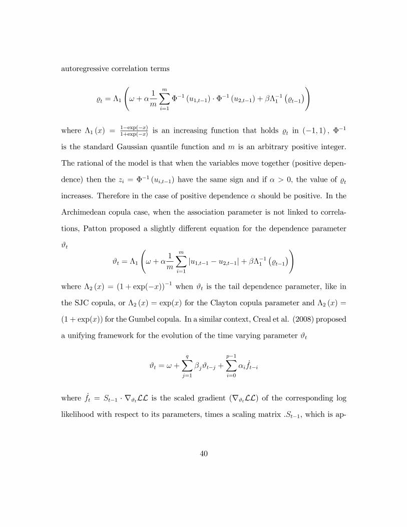
autoregressive correlation terms
%t = Λ1
(ω + α
1
m
m∑i=1
Φ−1 (u1,t−1) · Φ−1 (u2,t−1) + βΛ−11
(%t−1
))
where Λ1 (x) = 1−exp(−x)1+exp(−x)
is an increasing function that holds %t in (−1, 1) , Φ−1
is the standard Gaussian quantile function and m is an arbitrary positive integer.
The rational of the model is that when the variables move together (positive depen-
dence) then the zi = Φ−1 (ui,t−1) have the same sign and if α > 0, the value of %t
increases. Therefore in the case of positive dependence α should be positive. In the
Archimedean copula case, when the association parameter is not linked to correla-
tions, Patton proposed a slightly different equation for the dependence parameter
ϑt
ϑt = Λ1
(ω + α
1
m
m∑i=1
|u1,t−1 − u2,t−1|+ βΛ−11
(%t−1
))
where Λ2 (x) = (1 + exp(−x))−1 when ϑt is the tail dependence parameter, like in
the SJC copula, or Λ2 (x) = exp(x) for the Clayton copula parameter and Λ2 (x) =
(1 + exp(x)) for the Gumbel copula. In a similar context, Creal et al. (2008) proposed
a unifying framework for the evolution of the time varying parameter ϑt
ϑt = ω +
q∑j=1
βjϑt−j +
p−1∑i=0
αift−i
where ft = St−1 · ∇ϑtLL is the scaled gradient (∇ϑtLL) of the corresponding log
likelihood with respect to its parameters, times a scaling matrix .St−1, which is ap-
40
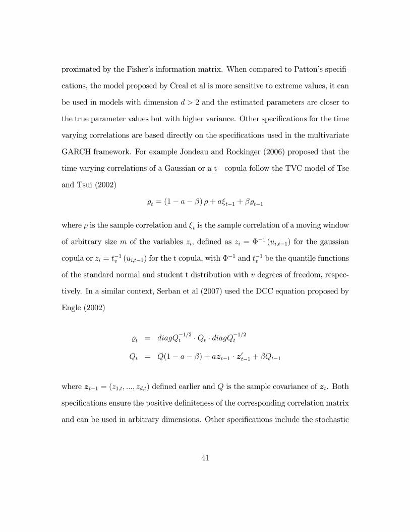
proximated by the Fisher’s information matrix. When compared to Patton’s specifi-
cations, the model proposed by Creal et al is more sensitive to extreme values, it can
be used in models with dimension d > 2 and the estimated parameters are closer to
the true parameter values but with higher variance. Other specifications for the time
varying correlations are based directly on the specifications used in the multivariate
GARCH framework. For example Jondeau and Rockinger (2006) proposed that the
time varying correlations of a Gaussian or a t - copula follow the TVC model of Tse
and Tsui (2002)
%t = (1− a− β) ρ+ aξt−1 + β%t−1
where ρ is the sample correlation and ξt is the sample correlation of a moving window
of arbitrary size m of the variables zi, defined as zi = Φ−1 (ui,t−1) for the gaussian
copula or zi = t−1v (ui,t−1) for the t copula, with Φ−1 and t−1
v be the quantile functions
of the standard normal and student t distribution with v degrees of freedom, respec-
tively. In a similar context, Serban et al (2007) used the DCC equation proposed by
Engle (2002)
%t = diagQ−1/2t ·Qt · diagQ−1/2
t
Qt = Q(1− a− β) + azt−1 · z′t−1 + βQt−1
where zt−1 = (z1,t, ..., zd,t) defined earlier and Q is the sample covariance of zt. Both
specifications ensure the positive definiteness of the corresponding correlation matrix
and can be used in arbitrary dimensions. Other specifications include the stochastic
41
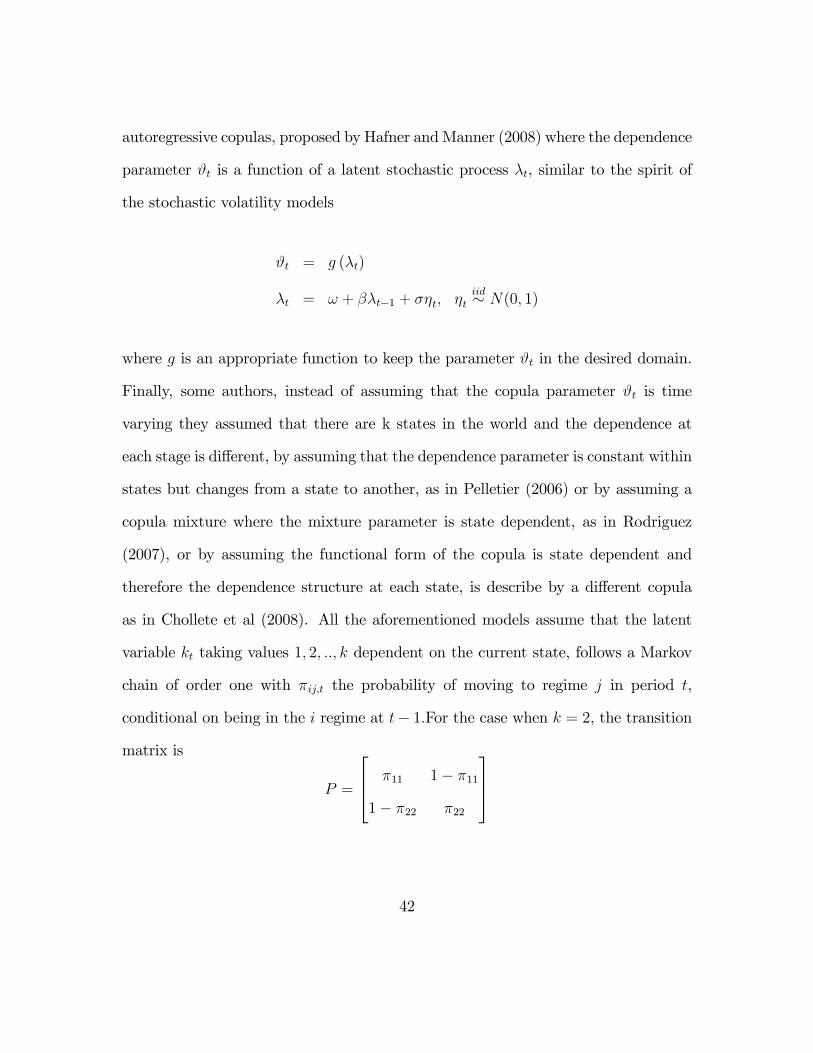
autoregressive copulas, proposed by Hafner andManner (2008) where the dependence
parameter ϑt is a function of a latent stochastic process λt, similar to the spirit of
the stochastic volatility models
ϑt = g (λt)
λt = ω + βλt−1 + σηt, ηtiid∼ N(0, 1)
where g is an appropriate function to keep the parameter ϑt in the desired domain.
Finally, some authors, instead of assuming that the copula parameter ϑt is time
varying they assumed that there are k states in the world and the dependence at
each stage is different, by assuming that the dependence parameter is constant within
states but changes from a state to another, as in Pelletier (2006) or by assuming a
copula mixture where the mixture parameter is state dependent, as in Rodriguez
(2007), or by assuming the functional form of the copula is state dependent and
therefore the dependence structure at each state, is describe by a different copula
as in Chollete et al (2008). All the aforementioned models assume that the latent
variable kt taking values 1, 2, .., k dependent on the current state, follows a Markov
chain of order one with πij,t the probability of moving to regime j in period t,
conditional on being in the i regime at t− 1.For the case when k = 2, the transition
matrix is
P =
π11 1− π11
1− π22 π22
42
now let ξt|t be the vector of probabilities of being in each state in the t−th period,
given the information at time t. Then
ξt|t =ξt|t−1 ηt
1′ξt|t−1 ηtξt+1|t = P ′ξt|t
LLC =
n∑t=1
log(1′ξt|t−1 ηt
)
where n is the sample size, 1′ is a vector of ones and ηt is the regime dependent quan-
tity of interest. The estimation procedure proposed for the above class of models is
called the expectation maximization (EM) algorithm and it is described in Hamilton
(1994). There are also other approaches proposed in the literature like ones that
assume structural breaks as in Dias and Embrechts (2004), the Local change point
method of Mercurrio and Spokoiny (2004) or the Adaptive estimation method of
Giacomini et al. For a review of these approaches the interested reader is referred to
Manner and Reznikova (2009).
43
Part II
The second part - Empirical
application
44
Chapter 2
Introduction
In this section I will try to quantify the dependence structure between some large
companys from the financial sector, listed in the S&P500 index and the index itself.
This is a fundamental problem in various areas of finance like risk management and
derivatives pricing since, both the risk (measured by the VaR of the CVaR of the
portfolio) and the price of a derivative written on a portfolio of assets, depend on the
distribution of the portfolio. Furthermore, my model can be seen as a time varying,
non normal version of the CAPM. The second part of the thesis is organized as
follows: Section (2.1) presents a literature review of the use of copulas and tries to
explain why copulas have become so popular in finance, section (2.2) describes the
proposed model in full detail and sections (2.3) to (2.5) compare the proposed with
other models and discuss the results and implications of the proposed model from
financial prespective. Section (2.6) concludes.
45
2.1 Literature review
In many financial applications, like portfolio selection, derivatives pricing and risk
management, the majority of the models used in practice, assume that the returns
distribution is multivariate normal and that the correlation among assets, which
is the measure of dependence in the multivariate normality framework, is constant
through time. For example, three of the most prominent financial applications,
Markowitz’s (1952) portfolio theory, portfolio Value at Risk (Morgan Stanley 1995)
and Black Merton and Scholes (1973) derivatives pricing theory, assume multivariate
normal returns and constant correlation. For more information the interested reader
is referred to Dowd (2001) or Jorion (1997).
However these two assumptions gained much criticism over the last years, since
they have failed to find any empirical support. Univariate financial time series share
some common characteristics, like heteroscedasticity, asymmetry and fat tails. The
univariate volatility structure is adequately described by the generalized autoregres-
sive conditional heteroscedasticity (GARCH) models of Bollerslev (1986) and its
extensions like the EGARCH model of Nelson (1991) and the asymmetric GARCH
model (GJR) of Glosten et al (1993), especially when these models are combined with
flexible distributions like the Skew-T distribution of Hansen (1994), as in Jondeau
and Rockinger (2006) or the SU-Normal distribution of Johnson’s (1949) system as
in Choi and Nam (2008). The interested reader in univariate GARCH models and
their extensions is referred to Terasvirta (2006) or Tsay (2002) and the references
therein. In the multivariate framework financial time series share some common
46
characteristics, like the tail dependence. Two series X and Y with distributions FX
and FY , are said to be tail dependent if the probability of an extreme co movement is
greater than zero. The measure of tail dependence, is the tail dependnece coeffi cient
λL = limu−→0+
Pr[Y 6 F−1
Y (u)|X 6 F−1X (u)
]For the lower tail, or:
λU = limu−→1−
Pr[Y > F−1
Y (u)|X > F−1X (u)
]For the upper tail.
Of course the definition of tail dependence can be extended to arbitrary dimen-
sions. In the same paper Embrechts, Mc Neil and Strautman prove that the multivari-
ate normal distribution does not exhibit any tail dependence, except of the extreme
case where % = 1. This means that under plausible conditions, the multivariate nor-
mal distribution assigns zero probability to extreme co movements therefore is not
able to describe financial returns. In a similar context, financial returns proved to
be not only tail dependent but asymmetric as well. By using extreme value theory
to model the tails of a multivariate distribution, Longin and Solnik (2001) showed
that correlations tend to increase in bear markets and decrease in bull markets, and
thus rejected the multivariate normality hypothesis. They proposed a measure of
47
this asymmetry named exceedance correlation defined as
Ex_Corr (X, Y, ϑ, φ) =
Corr(X, Y |X ≤ ϑ, Y ≤ φ) for ϑ, φ ≤ 0
Corr(X, Y |X ≥ ϑ, Y ≥ φ) for ϑ, φ ≥ 0
and they proved that, asymptotically, exceedance correlation is zero for large
positive returns and strictly positive for large negative returns. In a similar setting,
Ang and Chen (2002) showed that correlations between stocks are much greater in
downside moves than in upside moves. The existence of such stylized facts tends to
reject the normality hypothesis. Furthermore the constant correlations hypothesis
among financial returns failed to find empirical support, as in Engle and Sheppard
(2001) who proposed a test that failed to find support of constant correlation in
S&P500 portfolios. Constant correlation tests have also been proposed from Tse
(2000) and Berra and Kim (2001). Again, these test reviled that correlations among
assets tends to be time —varying.
To model this time varying dependence among financial returns, GARCH models
were extended to the multivariate setting. In the multivariate GARCH family belong
the vech model of Bollerslev, Engle and Wooldridge (1988), and its extension, the
diagonal vech however the vast number of estimated parameters and the complexity
of the conditions needed to ensure the positive —definiteness of the conditional co-
variance matrix make these models impractical, even for small dimensions. In order
to eliminate the problem of ensuring positive definiteness Engle and Kroner (1995)
proposed the BEKK model, which, in its general form, is also diffi cult to estimate,
48
since the number of estimated parameters is O(k4), where k is the dimension. In
order to minimize the number of estimated parameters and therefore the compu-
tational burden, Alexander (2000) proposed the orthogonal GARCH model, which
gave birth to a whole new class of models named factor GARCH models. The model
proposed by Alexander is a linear combination of univariate GARCH models under a
factor analysis framework. This model suffers from two limitations. It does not work
well in cases where the series are not highly correlated and it is diffi cult to interpret
the factors from a financial point of view. The multivariate GARCH model that
gained most of the attention and is now considered as the benchmark model is the
dynamic conditional correlation (DCC) model of Engle and Sheppard (2001). The
main advantage of DCC is that allows a two step estimation of the parameters, since
it decomposes correlation to variances and covariances. At the first step, working
independence among margins is assumed and the conditional variances are estimated
by univariate GARCH models. At the second step, the dynamic correlation is esti-
mated, conditional on the results of the first step. Furthermore, DCC ensures that
the estimated correlation matrices are positive definite under very mild conditions
and the number of the estimated parameters of the second step can be reduced down
to two, independent to the dimension of the series, therefore it can be estimated in
problems of very large dimensions . Silvennoinen and Terasvirta (2008) or Bauwens
et al (2006) give a complete overview of multivariate GARCH models.
The main criticism on multivariate GARCHmodels is that they estimated assum-
ing multivariate normality, although Bollerslev and Wooldridge (1992) showed that
the maximum likelihood estimations, assuming normality, are consistent, given that
49
both the conditional mean and conditional variance are specified correctly. Mul-
tivariate GARCH models that make non — normal distributional assumptions for
the residuals can be found in Pelagatti (2004) or Fiorentini et al (2003) where the
Student-T distribution is assumed or in Bauens and Laurent (2002) where the inno-
vations follow skew-T distribution. Nevertheless the use of any standard distribution
seldom fits the data well. If a returns process follows the Student —T distribution
with v degrees of freedom, each margin follows the Student-T distribution with v de-
grees of freedom and the joint distribution is also T with the same degrees of freedom,
an assumption that was found to be too restrictive in empirical applications.
The need for more flexible distributions that were able to better capture the char-
acteristics of financial distributions led the researchers to the use of copulas. Strictly
speaking a Copula is a d dimensional distribution function on [0, 1]d with standard
uniform margins. According to Sclar’s theorem (1959), if a multivariate distribution
has continuous margins there exists a unique copula that governs the dependence
structure, implied by the distribution. For example the t-copula represents the de-
pendence structure implied by the multivariate Student —T distribution. The main
advantage of copulas is that the joint distribution can be factored to the dependence
(the copula) and the margins. The marginal distributions are estimated separately
from the dependence, which is governed by the copula. Patton (2002) extended the
copula theory to cover the case of conditional multivariate distributions, allowing
the construction of flexible joint conditional distributions. The combination of the
conditional copulas and multivariate GARCH gave birth to a new class of models
named copula GARCH (CGARCH) models, which gained considerable popularity
50
the past few years. For example Jondeau and Rockinger (2006) apply this method-
ology to investigate the dependence between daily stock index returns. Serban et
al (2006) investigate the performance of a copula DCC model (a model with de-
pendence implied by the T-Copula and correlation dynamics implied by the DCC)
and they find it to be more effi cient that multivariate GARCH models. In a similar
setting Fantazzini used copula GARCH models to estimate the value at risk (VaR)
of various index portfolios, Patton (2006) investigates the asymmetric dependence
between exchange rates, while Ausin and Lopes (2006) used this setting to estimate
time varying multivariate distributions in a Bayesian framework.
Copulas are now considered to be the "industry standard" tool to quantify de-
pendence and are used in many financial applications. In the risk management
framework, recent implementations of copula theory can be found at Wang et al
(2010) where the VaR and CVaR of exchange rate portfolios are calculated for a bas-
ket of four international currencies, namely EUR, USD, JPY and HKD, or in Barges
et al (2009)where the problem of capital allocation under tail value at risk (TVaR,
Artzner et al 1999) is addressed. In a similar setting Perignon and Smith (2010)
study whether the diversification effect is underestimated as a possible explanation
to abnormal high levels of risk reported by international banks and its implications
to reserve capital requirements of a banking institution Finally Huang et al (2009)
propose a novel method to calculate the VaR of a portfolio based on copula GARCH
models and showed that the t - copula based estimations outperform classical ap-
proach in terms of VaR violations in all confidence levels. Copulas are also used to
quantify other sources of risk than market risk, like credit risk, as in Cousin and
51
Laurent (2008) or operational risk as in Chavez - Demoulin et al (2006).
In derivatives pricing Goorbergh et al (2005) is among the first who utilized copula
theory to price options written on S&P500 and Nazdaq indices. They conclude that
option prices implied by copula models differ significantly from those implied by the
standard Gaussian assumption. Similar results are obtained in Zhang and Guegan
(2008) where they conclude that prices obtained from a time varying t copula with
GARCH marginal processes are the optimum way to calculate prices for derivatives,
among their competing models. The pricing of derivatives issued on more than two
assets is the problem addressed in Bedento et al (2010) where options written on a
basket of five UK shares are studied. Their analysis reveals that results from copula
models differ significantly from the standard gaussian approaches only in volatile but
not in tranquil periods. Other authors, like Malo (2009) investigate the dependence
between spot and future electricity prices using Markov switching multifractal models
combined with copulas while Geman and Kharoubi (2009) study the assumption of
negatively correlated equity and commodity returns with copula models and find
that this assumption is mostly due to the Gaussian assumption previously used to
quantify dependencies. Finally Chen et al (2008) uses copula to study the dependence
structure between CDS’s (Credit Default Swap’s) and the kurtosis of equity returns
and observed that lower rating classes display positive and asymmetric dependence
structure unlike higher rating classes whose dependence structure seems to be almost
symmetric.
Another research area where copulas are extensively used in financial contagion
and the modern global financial crisis in general. The term financial contagion is used
52
to describe the interdependence between financial market and how a crisis originated
in some market can spread out to affect other markets as well. One of the first
studies of financial contagion is in Rodriguez (2007) who used copula models in a
regime switching setup to study the changing dependence between financial market
in periods of turmoil. In the same setting Aloiu et al (2010) and Kenourgios etal
(2010) examine the effect of the US and UK markets to those of BRIC countries
(Brasil, Russia India China) markets and found strong evidence of contagion.
2.2 Data and methodology
Let Rt = (rm, rs) be a bivariate random vector of log - returns of a stock (rs) traded
in a market, and the returns of the market (rm). The measure of market risk that the
stock berries is known as beta of the the stock and can be referred to as a measure
of the sensitivity of the asset’s returns to market returns. Beta is estimated with the
market model
rs − rf = a+ b (rm − rf ) + ε (2.1)
where rf is the risk free rate. The expectations on the market model derive the
model known as CAPM (Jack Treynor (1961, 1962), William Sharpe (1964), John
Lintner (1965a,b) and Jan Mossin (1966))
E(rs) = rf + b · E(rm − rf )
53
CAPM is one of the most extensively used models in finance. It holds that
b =cov(rm, rs)
var(rm)= corr(rm, rs) ·
√var(rs)
var(rm)
(2.2)
therefore, in order to estimate betas of stock the correlation between the stock and
the market and the variance of the stock need to be estimated in the highest possible
accuracy. Stock betas can be obtained by estimating the regression implied in (2.1)
however this approach has two serious limitations
• It is based on the normality assumption.
• It provides static (not time varying) beta estimates
In section (2.1) we saw that both of these assumptions are too restrictive in
real life situations. Instead we propose a different model based on copula functions,
named t copula GARCH model (tCGARCH). My model assumptions are:
• The returns of both the stock and the market exhibit significant departures
from Normality. More precisely, we assume that each series follows Hansen’s
Skew t distribution (Hansen, 1994), which can accommodate asymmetry and
kurtosis in returns with time varying variances modelled with a GARCH type
process.
• The dependence structure between each stock and the index is time varying
and it is modeled with a t - copula with static degrees of freedom and time
varying correlations that follow a specification similar to the DCC model of
Engle.
54
Our assumptions are similar to those in Jondeau and Rockinger (2006) with
only difference that time varying correlations are model with the TVC model in
Jondeau and Rockinger1 To estimate the betas of some major stock of the financial
sector during the modern crisis period, three models where estimated: A simple
market model implied by (2.1) a DCC GARCH model (that is a gaussian copula
with gaussian margins) and a tCGARCH model described earlier. The first model
provides static estimates for betas unlike the other two. The DCC model is used to
estimate time varying betas under the wrong assumption of normality. It is worth
noting that the tCGARCH model nest the DCC model, therefore both models can
be compared with standard likelihood tests or with an information criterion like BIC
or AIC. The aims of this empirical investigation are:
• To compare betas from the current period (2006 - 2010) to a less volatile
previous period (2002 - 2006) to see if the level or variablity of betas has
increased.
• To compare various models that are (or can be) used to calculate time varying
betas, in terms of their statistical accuracy
• To quantify the severity of model misspecification in risk management applica-
tions, by comparing the one step ahead VaR forecasts of the alternative models.
1I also estimated the model implied by Jondeau and Rockinger whoever log likelihood as wellas Akaike values are smaller in TVC than DCC in all cases that is why the DCC was my model ofchoice.
55
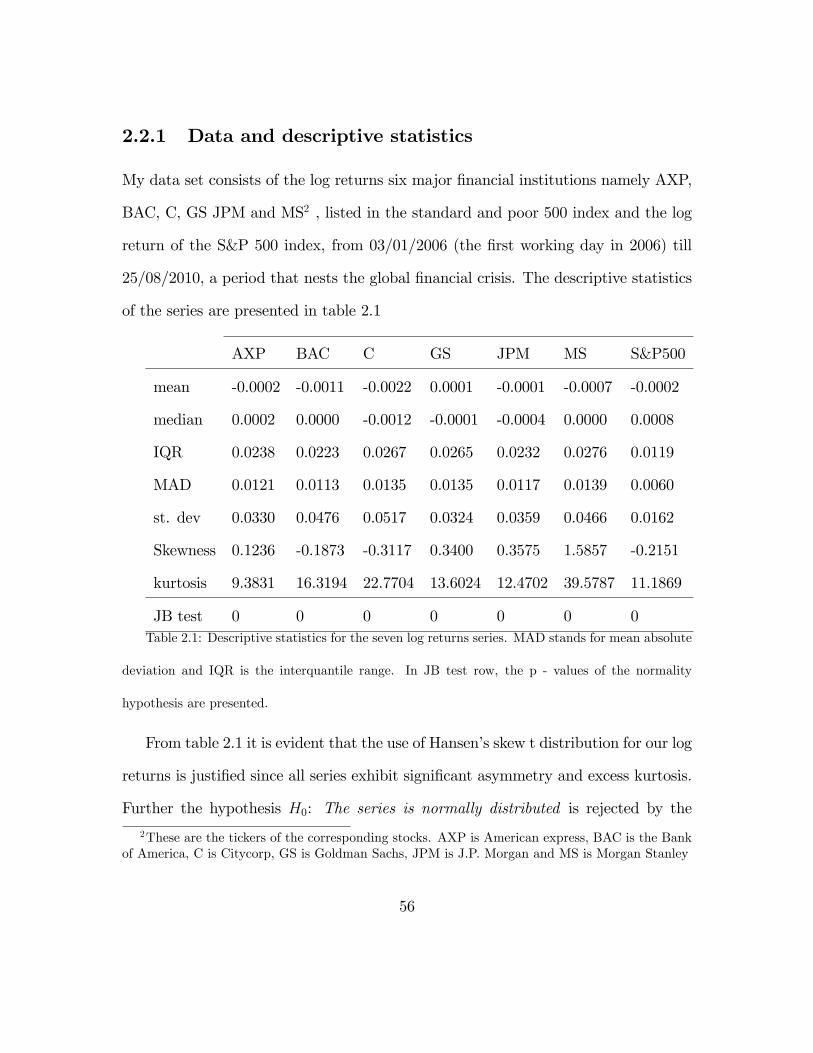
2.2.1 Data and descriptive statistics
My data set consists of the log returns six major financial institutions namely AXP,
BAC, C, GS JPM and MS2 , listed in the standard and poor 500 index and the log
return of the S&P 500 index, from 03/01/2006 (the first working day in 2006) till
25/08/2010, a period that nests the global financial crisis. The descriptive statistics
of the series are presented in table 2.1
AXP BAC C GS JPM MS S&P500
mean -0.0002 -0.0011 -0.0022 0.0001 -0.0001 -0.0007 -0.0002
median 0.0002 0.0000 -0.0012 -0.0001 -0.0004 0.0000 0.0008
IQR 0.0238 0.0223 0.0267 0.0265 0.0232 0.0276 0.0119
MAD 0.0121 0.0113 0.0135 0.0135 0.0117 0.0139 0.0060
st. dev 0.0330 0.0476 0.0517 0.0324 0.0359 0.0466 0.0162
Skewness 0.1236 -0.1873 -0.3117 0.3400 0.3575 1.5857 -0.2151
kurtosis 9.3831 16.3194 22.7704 13.6024 12.4702 39.5787 11.1869
JB test 0 0 0 0 0 0 0Table 2.1: Descriptive statistics for the seven log returns series. MAD stands for mean absolute
deviation and IQR is the interquantile range. In JB test row, the p - values of the normality
hypothesis are presented.
From table 2.1 it is evident that the use of Hansen’s skew t distribution for our log
returns is justified since all series exhibit significant asymmetry and excess kurtosis.
Further the hypothesis H0: The series is normally distributed is rejected by the
2These are the tickers of the corresponding stocks. AXP is American express, BAC is the Bankof America, C is Citycorp, GS is Goldman Sachs, JPM is J.P. Morgan and MS is Morgan Stanley
56
Jarque Berra test in all confidence levels.
2.3 Empirical results
In order to estimate the parameters of our six bivariate copulas we resort to the two
- step estimation method of Joe and Xu (1996) presented thoroughly in subsection
1.4.2. Each of the seven univariate returns series ri,t is modeled with a GARCH type
process as follows:
ri,t = c0,i + c1,iri,t−1 + εi,t
εi,t = εi,t√hi,t
hi,t = ωi + αiε2i,t−1 + βihi,t−1 + γiε
2i,t−1 · I (εi,t−1 < 0) (2.3)
εi,t ∼ iid ST (di, λi)
This is the GJR model of Glosten et al (1993) specifically designed to capture asym-
metric effects in conditional volatility process hi,t and ST (di, λi) is the univariate
skew t distribution of Hansen, with density:
fST (z; d, λ) =
bc(1 + 1d−2
(bz+a1−λ)2)−(d+1)/2
if z < −a/b
bc(
1 + 1d−2
(bz+a1+λ
)2)−(d+1)/2
if z ≥ −a/b(2.4)
57
where d and λ are the degree of freedom and asymmetry parameter, respectively,
and
a ≡ 4λcd− 2
d− 1, b ≡ 1 + 3λ2 − a2, c ≡
Γ(d+1
2
)Γ(d2
)√π (d− 2)
When λ = 0 Hansen’s Skew t distribution collapses to the central t - distribution
with d degrees of freedom. Further if both λ = 0 and d −→ ∞ the distribution
collapses the standard normal distribution, therefore this density nests the other two
densities that dominate the applications in GARCH processes. Having estimated
the marginal models independently, the standardized residuals are transformed to
uniform with the probability integral transformation
εi,t ∼ iid ST (di, λi) then ui,t = Fst (εi,t; di, λi) ∼ U(0, 1)
where Fst denotes the skew t cumulative distribution function. Having transformed
the standardized residuals to uniform, we create six bivariate data sets with uniform
margins, of the form ui,t, um,tTt=1 with i = AXP,BAC,C,GS, JPM,MS . To
each of the six data sets a t− copula with time varying correlations %t and static
58
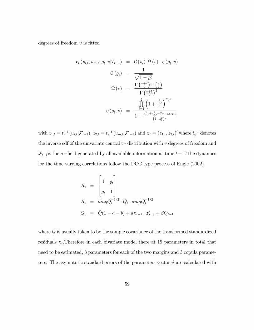
degrees of freedom v is fitted
ct (ui,t, um,t; %t, v|It−1) = C (%t) ·Ω (v) · η (%t, v)
C (%t) =1√
1− %2t
Ω (v) =Γ(v+2
2
)Γ(v2
)Γ(v+1
2
)2
η (%t, v) =
2∏i=1
(1 +
z2i,tv
) v+12
1 +z21,t+z
22,t−2%tz1,tz2,t
(1−%2t)v
with z1,t = t−1v (ui,t|Ft−1), z2,t = t−1
v (um,t|Ft−1) and zt = (z1,t, z2,t)′ where t−1
v denotes
the inverse cdf of the univariate central t - distribution with v degrees of freedom and
Ft−1is the σ−field generated by all available information at time t− 1.The dynamics
for the time varying correlations follow the DCC type process of Engle (2002)
Rt =
1 %t
%t 1
Rt = diagQ
−1/2t ·Qt · diagQ−1/2
t
Qt = Q(1− a− b) + azt−1 · z′t−1 + βQt−1
where Q is usually taken to be the sample covariance of the transformed standardized
residuals zt.Therefore in each bivariate model there at 19 parameters in total that
need to be estimated, 8 parameters for each of the two margins and 3 copula parame-
ters. The asymptotic standard errors of the parameters vector ϑ are calculated with
59
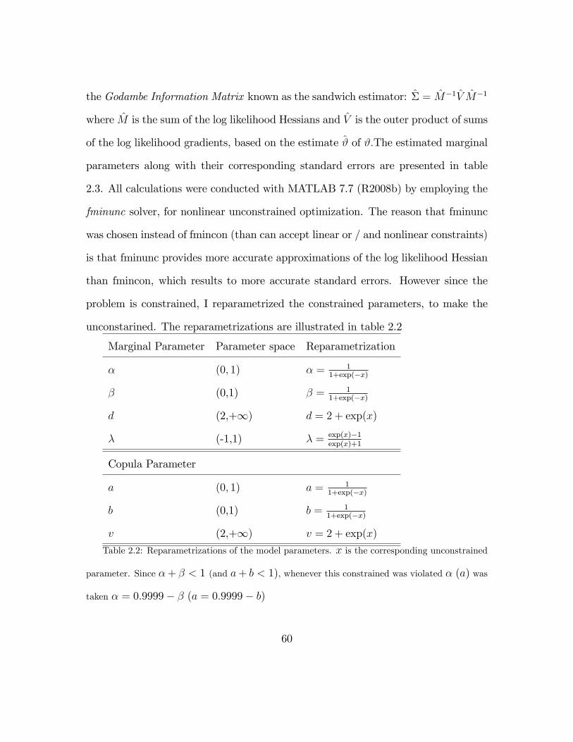
the Godambe Information Matrix known as the sandwich estimator: Σ = M−1V M−1
where M is the sum of the log likelihood Hessians and V is the outer product of sums
of the log likelihood gradients, based on the estimate ϑ of ϑ.The estimated marginal
parameters along with their corresponding standard errors are presented in table
2.3. All calculations were conducted with MATLAB 7.7 (R2008b) by employing the
fminunc solver, for nonlinear unconstrained optimization. The reason that fminunc
was chosen instead of fmincon (than can accept linear or / and nonlinear constraints)
is that fminunc provides more accurate approximations of the log likelihood Hessian
than fmincon, which results to more accurate standard errors. However since the
problem is constrained, I reparametrized the constrained parameters, to make the
unconstarined. The reparametrizations are illustrated in table 2.2
Marginal Parameter Parameter space Reparametrization
α (0, 1) α = 11+exp(−x)
β (0,1) β = 11+exp(−x)
d (2,+∞) d = 2 + exp(x)
λ (-1,1) λ = exp(x)−1exp(x)+1
Copula Parameter
a (0, 1) a = 11+exp(−x)
b (0,1) b = 11+exp(−x)
v (2,+∞) v = 2 + exp(x)
Table 2.2: Reparametrizations of the model parameters. x is the corresponding unconstrained
parameter. Since α+ β < 1 (and a+ b < 1), whenever this constrained was violated α (a) was
taken α = 0.9999− β (a = 0.9999− b)
60
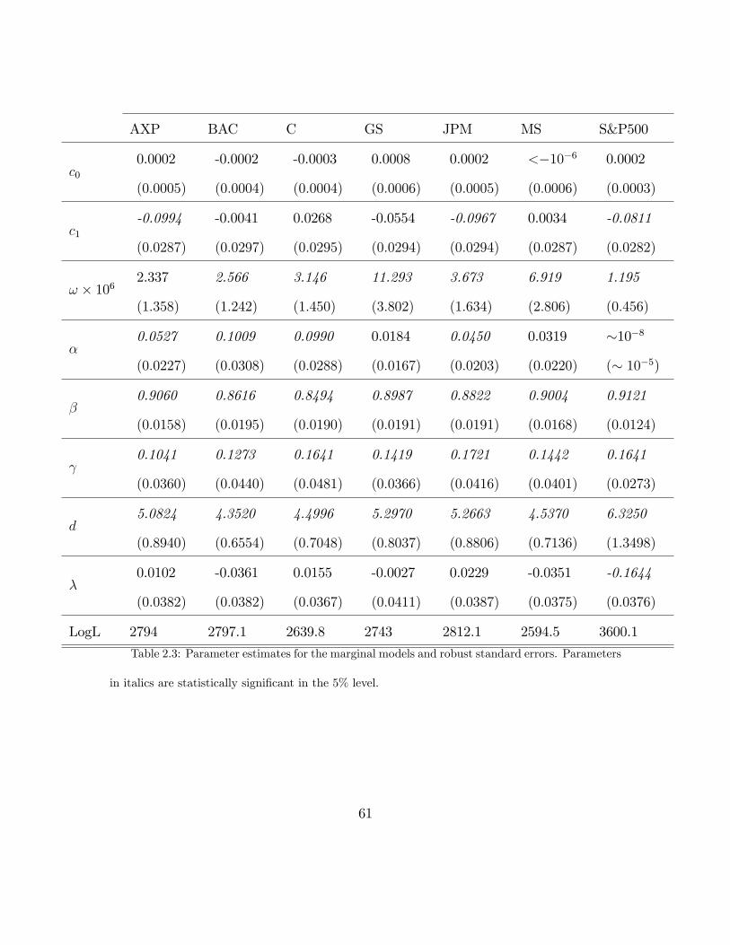
AXP BAC C GS JPM MS S&P500
c0
0.0002
(0.0005)
-0.0002
(0.0004)
-0.0003
(0.0004)
0.0008
(0.0006)
0.0002
(0.0005)
<−10−6
(0.0006)
0.0002
(0.0003)
c1
-0.0994
(0.0287)
-0.0041
(0.0297)
0.0268
(0.0295)
-0.0554
(0.0294)
-0.0967
(0.0294)
0.0034
(0.0287)
-0.0811
(0.0282)
ω × 1062.337
(1.358)
2.566
(1.242)
3.146
(1.450)
11.293
(3.802)
3.673
(1.634)
6.919
(2.806)
1.195
(0.456)
α0.0527
(0.0227)
0.1009
(0.0308)
0.0990
(0.0288)
0.0184
(0.0167)
0.0450
(0.0203)
0.0319
(0.0220)
∼10−8
(∼ 10−5)
β0.9060
(0.0158)
0.8616
(0.0195)
0.8494
(0.0190)
0.8987
(0.0191)
0.8822
(0.0191)
0.9004
(0.0168)
0.9121
(0.0124)
γ0.1041
(0.0360)
0.1273
(0.0440)
0.1641
(0.0481)
0.1419
(0.0366)
0.1721
(0.0416)
0.1442
(0.0401)
0.1641
(0.0273)
d5.0824
(0.8940)
4.3520
(0.6554)
4.4996
(0.7048)
5.2970
(0.8037)
5.2663
(0.8806)
4.5370
(0.7136)
6.3250
(1.3498)
λ0.0102
(0.0382)
-0.0361
(0.0382)
0.0155
(0.0367)
-0.0027
(0.0411)
0.0229
(0.0387)
-0.0351
(0.0375)
-0.1644
(0.0376)
LogL 2794 2797.1 2639.8 2743 2812.1 2594.5 3600.1
Table 2.3: Parameter estimates for the marginal models and robust standard errors. Parameters
in italics are statistically significant in the 5% level.
61
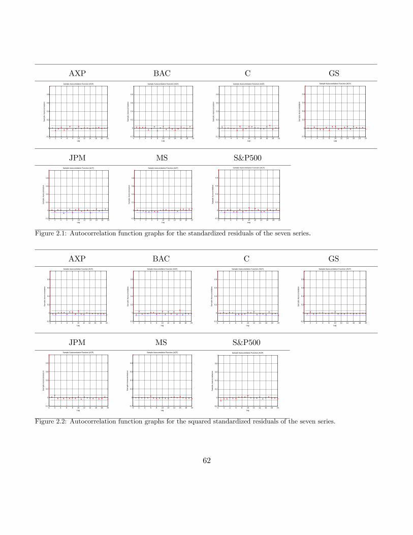
AXP BAC C GS
0 2 4 6 8 10 12 14 16 18 200.2
0
0.2
0.4
0.6
0.8
Lag
Sam
ple
Aut
ocor
rela
tion
Sample Autocorrelation Function (ACF)
0 2 4 6 8 10 12 14 16 18 200.2
0
0.2
0.4
0.6
0.8
Lag
Sam
ple
Aut
ocor
rela
tion
Sample Autocorrelation Function (ACF)
0 2 4 6 8 10 12 14 16 18 200.2
0
0.2
0.4
0.6
0.8
Lag
Sam
ple
Aut
ocor
rela
tion
Sample Autocorrelation Function (ACF)
0 2 4 6 8 10 12 14 16 18 200.2
0
0.2
0.4
0.6
0.8
Lag
Sam
ple
Aut
ocor
rela
tion
Sample Autocorrelation Function (ACF)
JPM MS S&P500
0 2 4 6 8 10 12 14 16 18 200.2
0
0.2
0.4
0.6
0.8
Lag
Sam
ple
Aut
ocor
rela
tion
Sample Autocorrelation Function (ACF)
0 2 4 6 8 10 12 14 16 18 200.2
0
0.2
0.4
0.6
0.8
Lag
Sam
ple
Aut
ocor
rela
tion
Sample Autocorrelation Function (ACF)
0 2 4 6 8 10 12 14 16 18 200.2
0
0.2
0.4
0.6
0.8
Lag
Sam
ple
Aut
ocor
rela
tion
Sample Autocorrelation Function (ACF)
Figure 2.1: Autocorrelation function graphs for the standardized residuals of the seven series.
AXP BAC C GS
0 2 4 6 8 10 12 14 16 18 200.2
0
0.2
0.4
0.6
0.8
Lag
Sam
ple
Aut
ocor
rela
tion
Sample Autocorrelation Function (ACF)
0 2 4 6 8 10 12 14 16 18 200.2
0
0.2
0.4
0.6
0.8
Lag
Sam
ple
Aut
ocor
rela
tion
Sample Autocorrelation Function (ACF)
0 2 4 6 8 10 12 14 16 18 200.2
0
0.2
0.4
0.6
0.8
Lag
Sam
ple
Aut
ocor
rela
tion
Sample Autocorrelation Function (ACF)
0 2 4 6 8 10 12 14 16 18 200.2
0
0.2
0.4
0.6
0.8
Lag
Sam
ple
Aut
ocor
rela
tion
Sample Autocorrelation Function (ACF)
JPM MS S&P500
0 2 4 6 8 10 12 14 16 18 200.2
0
0.2
0.4
0.6
0.8
Lag
Sam
ple
Aut
ocor
rela
tion
Sample Autocorrelation Function (ACF)
0 2 4 6 8 10 12 14 16 18 200.2
0
0.2
0.4
0.6
0.8
Lag
Sam
ple
Aut
ocor
rela
tion
Sample Autocorrelation Function (ACF)
0 2 4 6 8 10 12 14 16 18 200.2
0
0.2
0.4
0.6
0.8
Lag
Sam
ple
Aut
ocor
rela
tion
Sample Autocorrelation Function (ACF)
Figure 2.2: Autocorrelation function graphs for the squared standardized residuals of the seven series.
62
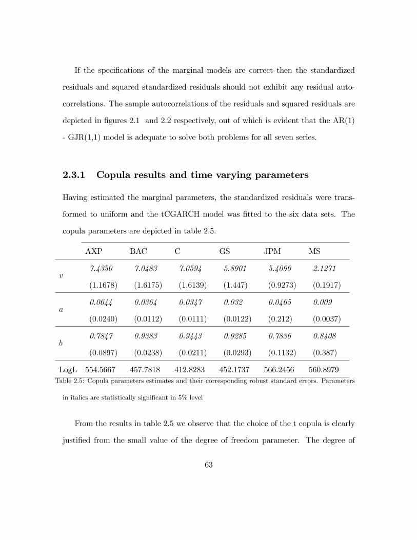
If the specifications of the marginal models are correct then the standardized
residuals and squared standardized residuals should not exhibit any residual auto-
correlations. The sample autocorrelations of the residuals and squared residuals are
depicted in figures 2.1 and 2.2 respectively, out of which is evident that the AR(1)
- GJR(1,1) model is adequate to solve both problems for all seven series.
2.3.1 Copula results and time varying parameters
Having estimated the marginal parameters, the standardized residuals were trans-
formed to uniform and the tCGARCH model was fitted to the six data sets. The
copula parameters are depicted in table 2.5.
AXP BAC C GS JPM MS
v7.4350
(1.1678)
7.0483
(1.6175)
7.0594
(1.6139)
5.8901
(1.447)
5.4090
(0.9273)
2.1271
(0.1917)
a0.0644
(0.0240)
0.0364
(0.0112)
0.0347
(0.0111)
0.032
(0.0122)
0.0465
(0.212)
0.009
(0.0037)
b0.7847
(0.0897)
0.9383
(0.0238)
0.9443
(0.0211)
0.9285
(0.0293)
0.7836
(0.1132)
0.8408
(0.387)
LogL 554.5667 457.7818 412.8283 452.1737 566.2456 560.8979Table 2.5: Copula parameters estimates and their corresponding robust standard errors. Parameters
in italics are statistically significant in 5% level
From the results in table 2.5 we observe that the choice of the t copula is clearly
justified from the small value of the degree of freedom parameter. The degree of
63
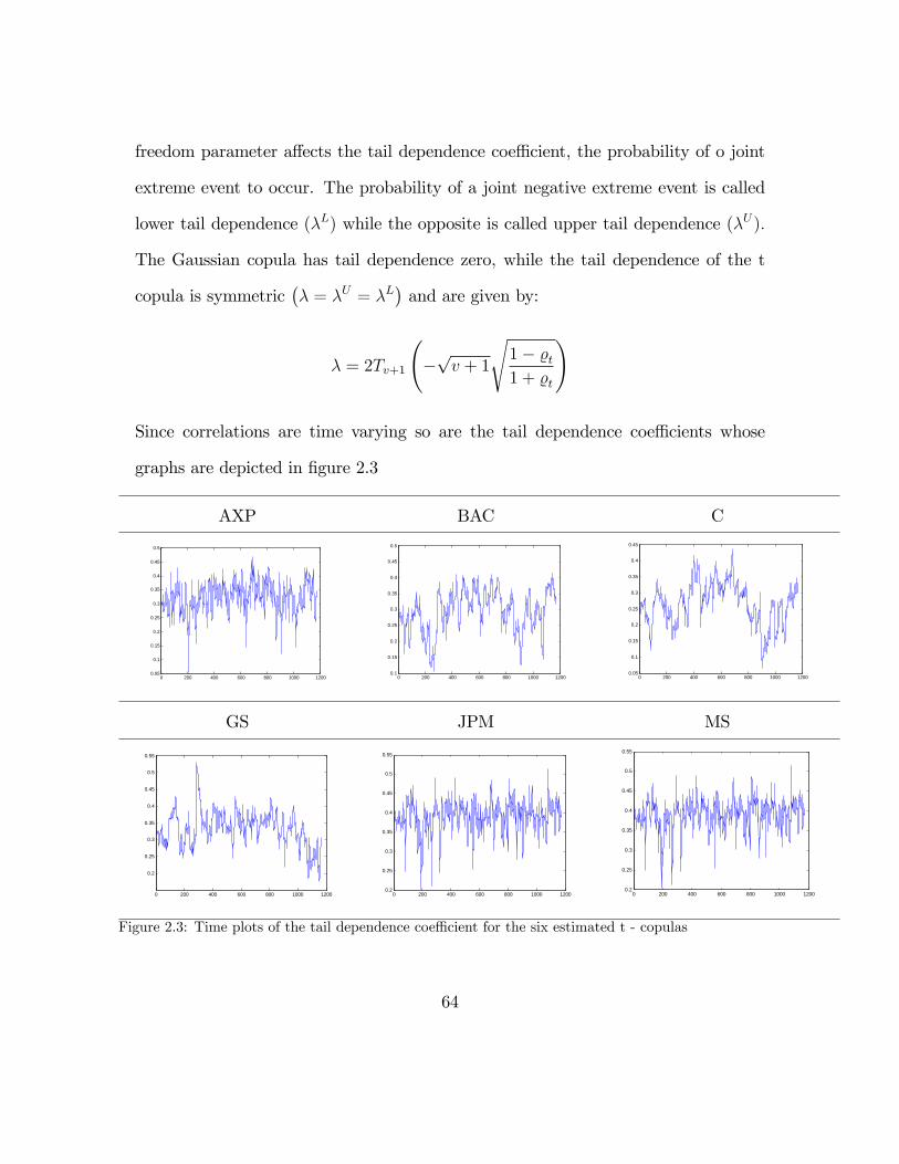
freedom parameter affects the tail dependence coeffi cient, the probability of o joint
extreme event to occur. The probability of a joint negative extreme event is called
lower tail dependence (λL) while the opposite is called upper tail dependence (λU).
The Gaussian copula has tail dependence zero, while the tail dependence of the t
copula is symmetric(λ = λU = λL
)and are given by:
λ = 2Tv+1
(−√v + 1
√1− %t1 + %t
)
Since correlations are time varying so are the tail dependence coeffi cients whose
graphs are depicted in figure 2.3
AXP BAC C
0 200 400 600 800 1000 12000.05
0.1
0.15
0.2
0.25
0.3
0.35
0.4
0.45
0.5
0 200 400 600 800 1000 12000.1
0.15
0.2
0.25
0.3
0.35
0.4
0.45
0.5
0 200 400 600 800 1000 12000.05
0.1
0.15
0.2
0.25
0.3
0.35
0.4
0.45
GS JPM MS
0 200 400 600 800 1000 1200
0.2
0.25
0.3
0.35
0.4
0.45
0.5
0.55
0 200 400 600 800 1000 12000.2
0.25
0.3
0.35
0.4
0.45
0.5
0.55
0 200 400 600 800 1000 12000.2
0.25
0.3
0.35
0.4
0.45
0.5
0.55
Figure 2.3: Time plots of the tail dependence coeffi cient for the six estimated t - copulas
64
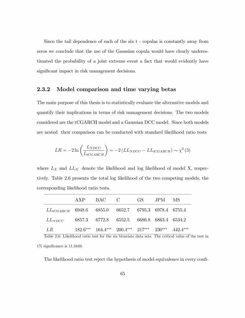
Since the tail dependence of each of the six t - copulas is constantly away from
zeros we conclude that the use of the Gaussian copula would have clearly underes-
timated the probability of a joint extreme event a fact that would evidently have
significant impact in risk management decisions.
2.3.2 Model comparison and time varying betas
The main purpose of this thesis is to statistically evaluate the alternative models and
quantify their implications in terms of risk management decisions. The two models
considered are the tCGARCH model and a Gaussian DCC model. Since both models
are nested their comparison can be conducted with standard likelihood ratio tests
LR = −2 ln
(LNDCC
LtCGARCH
)= −2 (LLNDCC − LLtCGARCH) ∼ χ2 (3)
where LX and LLX denote the likelihood and log likelihood of model X, respec-
tively. Table 2.6 presents the total log likelihood of the two competing models, the
corresponding likelihood ratio tests.
AXP BAC C GS JPM MS
LLtCGARCH 6948.6 6855.0 6652.7 6795.3 6978.4 6755.4
LLNDCC 6857.3 6772.8 6552.5 6686.8 6863.4 6534.2
LR 182.6∗∗∗ 164.4∗∗∗ 200.4∗∗∗ 217∗∗∗ 230∗∗∗ 442.4∗∗∗
Table 2.6: Likelihood ratio test for the six bivariate data sets. The critical value of the test in
1% significance is 11.3449.
The likelihood ratio test reject the hypothesis of model equivalence in every confi-
65
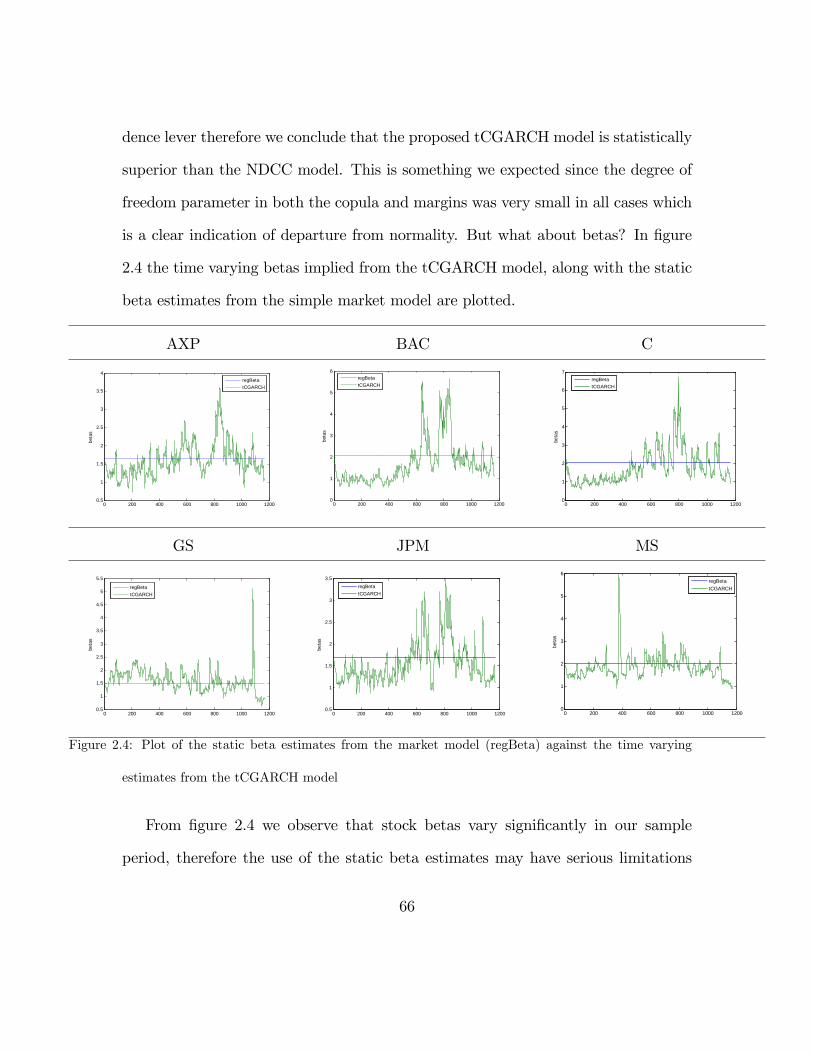
dence lever therefore we conclude that the proposed tCGARCH model is statistically
superior than the NDCC model. This is something we expected since the degree of
freedom parameter in both the copula and margins was very small in all cases which
is a clear indication of departure from normality. But what about betas? In figure
2.4 the time varying betas implied from the tCGARCH model, along with the static
beta estimates from the simple market model are plotted.
AXP BAC C
0 200 400 600 800 1000 12000.5
1
1.5
2
2.5
3
3.5
4
beta
s
regBetatCGARCH
0 200 400 600 800 1000 12000
1
2
3
4
5
6
beta
s
regBetatCGARCH
0 200 400 600 800 1000 12000
1
2
3
4
5
6
7
beta
s
regBetatCGARCH
GS JPM MS
0 200 400 600 800 1000 12000.5
1
1.5
2
2.5
3
3.5
4
4.5
5
5.5
beta
s
regBetatCGARCH
0 200 400 600 800 1000 12000.5
1
1.5
2
2.5
3
3.5
beta
s
regBetatCGARCH
0 200 400 600 800 1000 12000
1
2
3
4
5
6
beta
s
regBetatCGARCH
Figure 2.4: Plot of the static beta estimates from the market model (regBeta) against the time varying
estimates from the tCGARCH model
From figure 2.4 we observe that stock betas vary significantly in our sample
period, therefore the use of the static beta estimates may have serious limitations
66
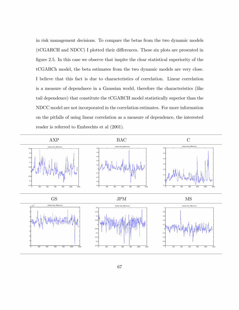
in risk management decisions. To compare the betas from the two dynamic models
(tCGARCH and NDCC) I plotted their differences. These six plots are presented in
figure 2.5. In this case we observe that inspite the clear statistical superiority of the
tCGARCh model, the beta estimates from the two dynamic models are very close.
I believe that this fact is due to characteristics of correlation. Linear correlation
is a measure of dependnece in a Gaussian world, therefore the characteristics (like
tail dependence) that constitute the tCGARCH model statistically superior than the
NDCCmodel are not incorporated in the correlation estimates. For more information
on the pitfalls of using linear correlation as a measure of dependence, the interested
reader is referred to Embrechts et al (2001).
AXP BAC C
0 200 400 600 800 1000 12000.15
0.1
0.05
0
0.05
0.1
0.15
0.2
0.25relative beta differences
0 200 400 600 800 1000 12000.4
0.3
0.2
0.1
0
0.1
0.2
0.3
0.4
0.5relative beta differences
0 200 400 600 800 1000 12000.1
0
0.1
0.2
0.3
0.4
0.5
0.6relative beta differences
GS JPM MS
0 200 400 600 800 1000 12005
4
3
2
1
0
1
2
3x 10⁶ relative beta differences
0 200 400 600 800 1000 12000.25
0.2
0.15
0.1
0.05
0
0.05
0.1
0.15
0.2relative beta differences
0 200 400 600 800 1000 12000.8
0.6
0.4
0.2
0
0.2
0.4
0.6
0.8
1relative beta differences
67
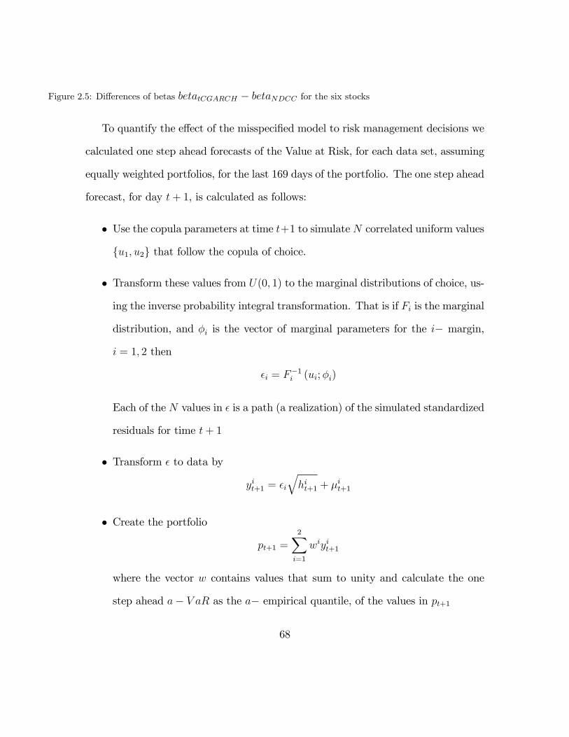
Figure 2.5: Differences of betas betatCGARCH − betaNDCC for the six stocks
To quantify the effect of the misspecified model to risk management decisions we
calculated one step ahead forecasts of the Value at Risk, for each data set, assuming
equally weighted portfolios, for the last 169 days of the portfolio. The one step ahead
forecast, for day t+ 1, is calculated as follows:
• Use the copula parameters at time t+1 to simulate N correlated uniform values
u1, u2 that follow the copula of choice.
• Transform these values from U(0, 1) to the marginal distributions of choice, us-
ing the inverse probability integral transformation. That is if Fi is the marginal
distribution, and φi is the vector of marginal parameters for the i− margin,
i = 1, 2 then
εi = F−1i (ui;φi)
Each of the N values in ε is a path (a realization) of the simulated standardized
residuals for time t+ 1
• Transform ε to data by
yit+1 = εi
√hit+1 + µit+1
• Create the portfolio
pt+1 =2∑i=1
wiyit+1
where the vector w contains values that sum to unity and calculate the one
step ahead a− V aR as the a− empirical quantile, of the values in pt+1
68
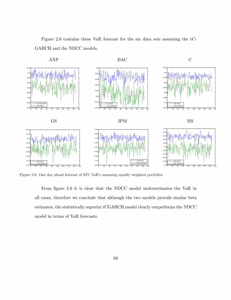
Figure 2.6 contains these VaR forecast for the six data sets assuming the tC-
GARCH and the NDCC models.
AXP BAC C
0 20 40 60 80 100 120 140 160 1800.034
0.032
0.03
0.028
0.026
0.024
0.022
0.02
0.018
VaR tCGARCHVaR NDCC
0 20 40 60 80 100 120 140 160 1800.034
0.032
0.03
0.028
0.026
0.024
0.022
0.02
VaR NDCCVaR tCGARCH
0 20 40 60 80 100 120 140 160 1800.075
0.07
0.065
0.06
0.055
0.05
0.045
0.04
0.035
VaR NDCCVaR tCGARCH
GS JPM MS
0 20 40 60 80 100 120 140 160 1800.032
0.03
0.028
0.026
0.024
0.022
0.02
0.018
0.016
VaR NDCCVaR tCGARCH
0 20 40 60 80 100 120 140 160 1800.032
0.03
0.028
0.026
0.024
0.022
0.02
0.018
0.016
VaR NDCCVaR tCGARCH
0 20 40 60 80 100 120 140 160 1800.04
0.038
0.036
0.034
0.032
0.03
0.028
0.026
0.024
0.022
0.02
VaR NDCCVaR tCGARCH
Figure 2.6: One day ahead forecast of 95% VaR’s assuming equally weighted portfolios
From figure 2.6 it is clear that the NDCC model underestimates the VaR in
all cases, therefore we conclude that although the two models provide similar beta
estimates, the statistically superior tCGARCH model clearly outperforms the NDCC
model in terms of VaR forecasts.
69
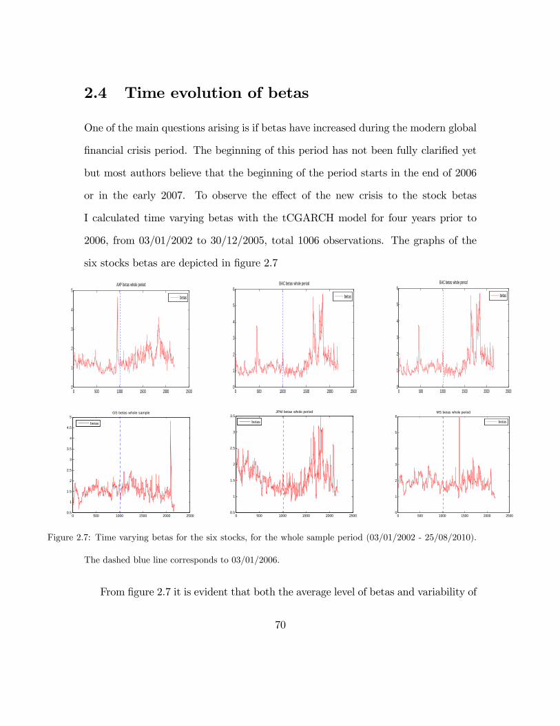
2.4 Time evolution of betas
One of the main questions arising is if betas have increased during the modern global
financial crisis period. The beginning of this period has not been fully clarified yet
but most authors believe that the beginning of the period starts in the end of 2006
or in the early 2007. To observe the effect of the new crisis to the stock betas
I calculated time varying betas with the tCGARCH model for four years prior to
2006, from 03/01/2002 to 30/12/2005, total 1006 observations. The graphs of the
six stocks betas are depicted in figure 2.7
0 500 1000 1500 2000 25000
1
2
3
4
5AXP betas whole period
betas
0 500 1000 1500 2000 25000
1
2
3
4
5
6BAC betas whole period
betas
0 500 1000 1500 2000 25000
1
2
3
4
5
6BAC betas whole period
betas
0 500 1000 1500 2000 25000.5
1
1.5
2
2.5
3
3.5
4
4.5
5GS betas whole sample
betas
0 500 1000 1500 2000 25000.5
1
1.5
2
2.5
3
3.5JPM betas whole period
betas
0 500 1000 1500 2000 25000
1
2
3
4
5
6MS betas whole period
betas
Figure 2.7: Time varying betas for the six stocks, for the whole sample period (03/01/2002 - 25/08/2010).
The dashed blue line corresponds to 03/01/2006.
From figure 2.7 it is evident that both the average level of betas and variability of
70
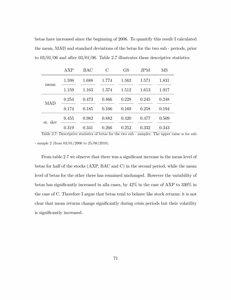
betas have increased since the beginning of 2006. To quantify this result I calculated
the mean, MAD and standard deviations of the betas for the two sub - periods, prior
to 03/01/06 and after 03/01/06. Table 2.7 illustrates these descriptive statistics
AXP BAC C GS JPM MS
mean1.598
1.159
1.688
1.163
1.774
1.374
1.562
1.512
1.571
1.613
1.831
1.917
MAD0.254
0.174
0.473
0.185
0.466
0.166
0.228
0.169
0.245
0.258
0.248
0.194
st. dev0.455
0.319
0.982
0.341
0.882
0.266
0.420
0.252
0.477
0.332
0.509
0.343Table 2.7: Descriptive statistics of betas for the two sub - samples. The upper value is for sub
- sample 2 (from 03/01/2006 to 25/08/2010).
From table 2.7 we observe that there was a significant increase in the mean level of
betas for half of the stocks (AXP, BAC and C) in the second period, while the mean
level of betas for the other three has remained unchanged. However the variability of
betas has significantly increased in alla cases, by 42% in the case of AXP to 330% in
the case of C. Therefore I argue that betas tend to behave like stock returns; it is not
clear that mean returns change significantly during crisis periods but their volatility
is significantly increased.
71
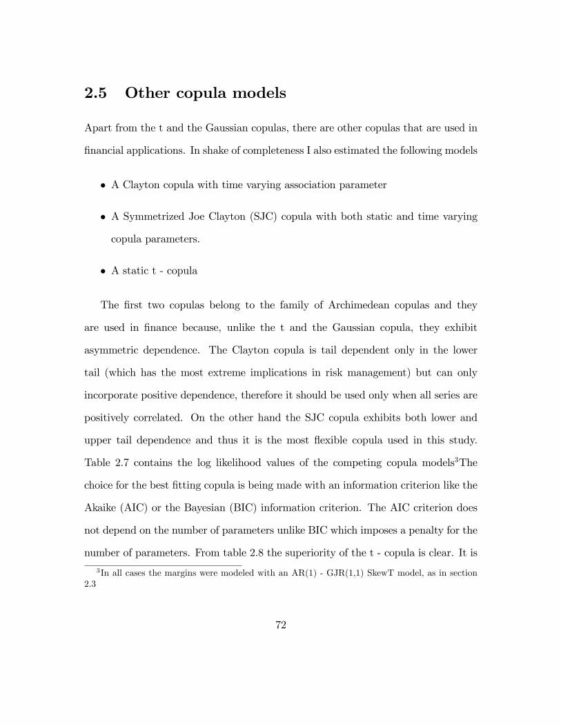
2.5 Other copula models
Apart from the t and the Gaussian copulas, there are other copulas that are used in
financial applications. In shake of completeness I also estimated the following models
• A Clayton copula with time varying association parameter
• A Symmetrized Joe Clayton (SJC) copula with both static and time varying
copula parameters.
• A static t - copula
The first two copulas belong to the family of Archimedean copulas and they
are used in finance because, unlike the t and the Gaussian copula, they exhibit
asymmetric dependence. The Clayton copula is tail dependent only in the lower
tail (which has the most extreme implications in risk management) but can only
incorporate positive dependence, therefore it should be used only when all series are
positively correlated. On the other hand the SJC copula exhibits both lower and
upper tail dependence and thus it is the most flexible copula used in this study.
Table 2.7 contains the log likelihood values of the competing copula models3The
choice for the best fitting copula is being made with an information criterion like the
Akaike (AIC) or the Bayesian (BIC) information criterion. The AIC criterion does
not depend on the number of parameters unlike BIC which imposes a penalty for the
number of parameters. From table 2.8 the superiority of the t - copula is clear. It is
3In all cases the margins were modeled with an AR(1) - GJR(1,1) SkewT model, as in section2.3
72
the superior copula in all sets for both criteria. The tCGARCH model is found to
be the best model in three cases according to the BIC and in five cases according to
the AIC, while the static t - copula is the best fitting copula, when the tCGARCH
isn’t.
AXP BAC C GS JPM MS
SJC tv
6 parameters
543.296 449.795 403,706 451.810 554.872 558.758
Clayton tv
3 parameters
449.675 381.201 342.541 379.99 474.9 481.42
t static
1 parameter
551.735 443.222 395.803 444.5 563.766 562.031
SJC static
2 parameters
533.566 437.067 388.443 443.111 542.445 527.918
tCGARCH
3 parameters
554.5671 457.7821 412.8281 452.1741 566.2461 560.898
Table 2.8: Loglikelihood values of the five alternative copula models. Values in boldface letters denote
the best fitting copula, according to Bayesian information criterion while values with thesuperscript 1 are
the best fitting copula according to Akaike information criterion
2.6 Conclusion
The multivariate distribution of a portfolio plays a significant role in finance since a
number of theories are based upon the statistical characteristics of the returns series.
73
In the univariate setting there are many distributions that seem to fit financial data
adequately however this is not the case when the problem in hand is multivariate. In
fact none of the existing multivariate distributions can accommodate all character-
istics of financial data. The remedy to this problem is to separate the multivariate
distribution to the marginal distributions and the dependence structure which is
described by a copula. This decomposition allows researcher to use different para-
metric models for the dependence and the margins that significantly adds flexibility
to the model. For example a multivariate t distribution enforces both the margins
and the dependence to have the same degree of freedom parameter which is rather
unrealistic. Instead one could use a t - copula with t - margins to allow all margins
and the copula to have their own degree of freedom parameter. This study aimed to
measure stock betas of some major financial institutions during the contemporary
period of global financial crisis by applying the results of copula theory, investigate
the implications of the proposed model in risk management applications and com-
pare the betas of the current regime to previous, less volatile periods.. The proposed
methodology, unlike traditional models, does not suffer from two serious limitations:
It does not assume normality and it can provide time varying beta calculations,
unlike the standard methodology used to calculate betas (the market model). I es-
tablished the statistical superiority of the proposed modeling scheme in comparison
with other sophisticated models used in finance and I concluded that, although the
proposed model provides similar results to other models that are based on the wrong
assumption of normality, it should be the model of choice when risk management
decisions are involved, since traditional models clearly underestimate the risk of the
74
portfolio, in comparison with the tCGARCH model. Further I provided empirical
evidence that betas behave like stock returns in terms of behavior during periods of
crisis. Even though the mean level of betas does not change during turmoil periods,
the variability of betas (like stock volatility) is significantly increased.
References
1. Aas, K., Haff, H., (2006), "The generalized hyperbolic Skew Student’s t distri-
bution." Journal of financial econometrics, 4 (2), 275 —309..
2. Alexander, C., (2000), "Orthogonal GARCH." Mastering risk volume 2.
3. Aloui R., Mohamed Safouane Ben Aissa, Duc Khuong Nguyen (2010), "Global
Financial crisis, extreme interdependences, and contagion effects: The role of
economic structure?" Journal of Banking & Finance (forthcoming)
4. Andersen, E.W. (2003), "Composite likelihood and two stage estimation in
family studies". Biostatistics 5, 15 —30.
5. Ausin, M.C., Lopez, H., (2009), "Time —varying joint distribution through
copulas." Computational statistics and data analysis, article in press.
6. Barges M., Helene Cossette, Etienne Marceau, (2009), "TVaR-based allocation
with copulas.", Insurance:Mathematics and Economics
75
7. Bartram S. M., Stephen J. Taylor, Yaw-Huei Wang, (2006), "The Euro and
European financial market dependence.", Journal of Banking & Finance
8. Bawens, L., Laurent, S., (2002), "A new class of multivariate skew densities,
with application to GARCH models." Journal of business and economic sta-
tistics.
9. Bawens, L., Laurent, S., Rombouts, J., (2006), "Multivariate GARCH models:
A survey." Journal of applied econometrics, 21, 79 —109
10. BedendoM., Francesca Campolongo, Elisabeth Joossens, Francesco Saia (2009),
"Pricing multiasset equity options:How relevant is the dependence function?"
Journal of Banking & Finance. 34 788-801
11. Bera, A.K., Kim, S., (2002), "Testing constancy of correlationand other speci-
fications of the BGARCH model." Working paper, CORE.
12. Besag, J.E. (1974), "Spatial interaction and the statistical analysis of lattice
systems." Journal of Royal statistical society, Series B (Methodological), 34,
192 —236.
13. Bessler, D. A., Yang, J. (2003). "The structure of interdependence in inter-
national stock markets." Journal of international money and finance 22, 261 -
287
14. Black, F., Scholes, M., (1973), "The Pricing of Options and Corporate Liabili-
ties". Journal of Political Economy 81 (3), 637—654.
76
15. Bollerslev, T., Engle, R., Wooldridge, J.M., (1988) "A capital asset pricing
model with time —varying covariances", The journal of political economy, 96,
116 —131.
16. Bollerslev, T., (1986), "Generalized autoregressive conditional heteroscedastic-
ity." Journal of Econometrics 31 (3), 307 - 327
17. Bollerslev, T., Wooldridge, J.M., (1992), "Quasi —maximum likelihood and
inference in dynamic models with time —varying covariances." Econometric
reviews 11 (2), 143 —172.
18. Berndt,E.K. Hall, B.H. and Hall, R.E. (1974) "Estimation and Inference in
Nonlinear Structural Models." Annals of Economic and Social Measurement,
Vol 3, (4)
19. Caporin, M., Mc Aleer, M., (2006), "Dynamic asymmetric GARCH." Journal
of financial econometrics, 4 (3), 385 —412.
20. Chan, Y., Li, H., (2008) "Tail dependence for multivariate t - copulas and its
monotonicity." Insurance: Mathematics and Economics, Vol42 (2), 763-770
21. Chavez-Demoulin V., P. Embrects, J. Neslehova, (2005), "Quantitative mod-
els for operational risk:Extremes, dependence and aggregation.", Journal of
Banking & Finance 30 2635-2658
22. Cherubini, U., Luciano, E., Vecchiato, W., (2004), "Copula methods in fi-
nance." John Wiley and sons, London.
77
23. Chen X., Fan, Y (2006) "Estimation and model selection of semiparamet-
ric copula-based multivariate dynamic models under copula misspecification"
Journal of Econometrics, 135, 1-2, 125-154
24. Chen, X, Wu, W.B., Yi, Y., (2009) "Effi cient estimation of copula-based semi-
parametric Markov models." Annals of statistics, vol 37 (6B), 4214-4253.
25. Chen Y.H., Anthony H. Tu, Kehluh Wang (2006), "Dependence structure be-
tween the credit default swap return and the kurtosis of the equity return dis-
tribution: Evidence from Japan.", Journal of International financial markets,
institutions & money 18 259-271
26. Chollete, L., Heinen, A., Valdesogo, A., (2009), "Modeling international finan-
cial returns with a multivariate regime switching copula." Journal of financial
econometrics, 7 (4), 437 - 480.
27. Cousin A., Jean - Paul Laurent (2008), "Comparison results for exchangeable
credit risk portfolios.", Insurance: Mathematics and Economics.42 1118-1127
28. Creal, D., Koopman, S.J. and Lucas, A., (2010) "A general framework for ob-
servation driven time varying parameter models." Discussion paper, Tinbergen
university.
29. Davison, A,C., Smith, R.L., (1990), "Models for exceedances over high thresh-
olds." Journal of Royal statistical society, Series B (Methodological), 52 (3),
393 —442.
78
30. Demarta, S., Mc Neil, A., (2005), "The t —copula and related copulas." Inter-
national statistical review, 73 (1), 111 —129.
31. Diamantopoulos, K., Vrontos, D., (2010) "A student - t full factor multivariate
GARCH model." Computational economics 35 (1), 63 - 83
32. Dias, A. (2004) "Copula inference for finance and insurance." PhD thesis, ETH
Zurich
33. Dias, A., Embrechts, P., (2004). "Dynamic copula models for multivariate high
frequency data in finance." ETH working paper.
34. Dowd, K. (2001), "Measuring Market Risk", John Wiley and sons.
35. Durrelman, V., Nikeghbali, A., Roncalli, T., (2000), "A simple transformation
of copulas." Technical report, Credit Lyonnais.
36. Engle, R.F., (2002), "Dynamic Conditional Correlation: A simple class of
multivariate generalized autoregressive conditional heteroscedasticity models."
Journal of business and economic statistics, 20, 339 —350.
37. Engle R.F., Kroner, K. F., (1995), "Multivariate simultaneous generalized
ARCH.", Econometric theory, 11, 122 —150.
38. Engle, R.F., Sheppard, K., (2001), "Theoretical and empirical properties of
dynamic conditional correlation multivariate GARCH." NBER working paper
8554
79
39. Engle, R.F., Shephard, N., Sheppard, K., (2008), "Fitting vast time —varying
covariance models." Draft paper, SSRN.
40. Embrechts, P., Mc Neil, A., Straumann, D., (2001). "Correlation and depen-
dence in risk management: Properties and Pitfalls." Risk management: value
at risk and beyond. Cambridge university press.
41. Fantazzini, D., (2008), "Dynamic Copula modeling for Value at Risk." Frontiers
in finance and economics, 5 (2), 72 —108.
42. Fermanian, J.D. and Scailet, O. (2004) "Some statistical pitfalls in copula
modeling for financial applications." "FAME research paper series, rp 108.
43. Fermanian, J.D. and Wegkamp, M.J. (2004) "Time dependent copulas."Work-
ing paper, centre de researche en economie et en statistique, Paris France
44. Fernandez, V., (2008) "Copula-based measures of dependence structure in as-
sets returns." Physica A: Statistical Mechanics and its Applications, Vol 387
(14), 3615-3628
45. Fiorentini G., Sentana E., CalzolariG., (2003), "Maximum likelihood estima-
tion and inference in multivariate conditionally heteroscedastic dynamic re-
gression models with Student t innovations." Journal of business and economic
statistics 21, 532 —546.
80
46. Glosten, R.T., Jagannathan, R., Runkle, D., (1993), "On the relation between
the expected value and the volatility of the nominal excess return on stocks."
Journal of finance 48 (5), 1779 —1801
47. Geman H., Cecile Kharoubi(2008), "WTI crude oil Futures in portfolio diver-
sification:The time -to-maturity effect.", Journal of Banking and Finance
48. Genest, C., Mackay, J., (1986). " The joy of copulas: bivariate distributions
with uniform marginals". American statisticial, vol 40, number 4.
49. Genest, C., Ghoudi, K., Rivest, L., (1995), "A semi —parametric estimation
procedure of dependence parameters in multivariate families of distributions."
Biometrica 82, 543 —552.
50. Genest, C., Verret, F., (2005) "Locally most powerful rank tests of indepen-
dence for copula models." Journal of nonparametric statistics, vol 17 (5), 521
—539
51. Genest, C., Quessy, J.F. and Remillard, B. (2006) "Goodness-of-fit Procedures
for Copula Models Based on the Probability Integral Transformation." Scan-
dinavian Journal of Statistics, 33 (2), 337-366
52. Genest, C. and Favre, A. (2007). "Everything you always wanted to know
about copula modeling but were affraid to ask." Journal of hydrologic engi-
neering, 12 (4), 347 - 368
81
53. Genest, C., Gendron, M., Bourdeau - Brien, M., (2009). "The Advent of
Copulas in Finance." The European journal of finance.
54. Giacomini, E., Hardle, W., Ignatieva,E., and Spokoiny, V., (2006) "Inhomo-
geneous dependency modeling with time varying copula." SFB 649 discussion
paper
55. Hamilton, J.D. (1994) "Time series analysis." Princeton university press, Prince-
ton
56. Hansen, B.E. (1994),"Autoregressive conditional density estimation." Interna-
tional Economic Review 35 (3), 705 —730
57. Huang, J.J., Lee, K.J., Liang, H., and Lin, W.F., (2009) "Estimating value at
risk of portfolio by conditional copula-GARCH method." Insurance: Mathe-
matics and economics, 45 (3), 315 - 324
58. Hult, H., Lindskog, F., (2002), ‘Multivariate extremes, Aggregation and De-
pendence in Elliptical Distributions.’Advances in Applied Probability, 34 (3),
587 —608
59. Hurlimann V., (2004). "Fitting bivariate cumulative returns with copulas."
Computational statistics and data analysis 45, 355 - 372 .
60. Joe, H., (1996,1997), "Multivariate models and dependence concepts." Chap-
man and Hall, London.
82
61. Johnson, N.L., (1949), "Systems of frequency curves generated by method of
translation." Biometrica 36, 149 —176.
62. Jondeau, E. and Rockinger, M. (2006),"The Copula —GARCH modelof con-
ditional dependencies: An international stock market application.", Journal of
International money and finance, 25, 827 —853.
63. Jorion, P. (1997), "Value at risk: The new benchmark for managing financial
risk", MC Grow —Hill
64. Kenourgios D., Ar. Samitas, N.Paltalidis (2010), "Financial c rises and stock
market contagion in a multivariate time-varying asymmetric framework.". Jour-
nal of International Financial Markets, Institutions & Money
65. Kim, G., Silvapulle, M.J., Silvapulle, P. (2007). "Comparison of semiparamet-
ric and parametric methods for estimating copulas." Computational statistics
and data analysis 51, 2386 - 2850.
66. Kole, E., Koedijk, K., Verbeek, M., (2007), "Selecting copulas for risk manage-
ment." Journal of banking and finance, 31 (8), 2405 —2423.
67. Kumar M.S., Tatsuyoshi Okimoto (2010), "Dynamics of International inte-
gration of government securities’markets.", Journal of Banking & Finance
forthcoming
83
68. Liu, Y. and Luger R., (2009) "Effi cient estimation of copula GARCH models."
Computational statistics and data analysis 53, 2284 - 2297
69. Longin, F., Solnik, B., (1995), "Is the correlation in equity markets constant:
1960 —1990?" Journal of International money and finance 14 (1), 3 —26.
70. Malo P., (2009), "Modeling electricity spot and futures price dependence:A
multifrequency approach.", Physica A 388 4763-4779
71. Manner, H., Reznikova, O., (2009) "Time varying copulas: A survey" IAP
statistical network : http://www.stat.ucl.ac.edu/IAP
72. Markowitz, H.M. (1952), "Portfolio Selection". The Journal of Finance 7 (1),
77—91.
73. Mashal, R., Zeevi,A. (2002). "Beyond correlation: Extreme co - movements
between financial assets."Working paper, Columbia graduate school of business.
74. Mendez, B., Souza, R. (2004). "Measuring financial risks with copulas." Inter-
national review of financial analysis 13, 27 - 45 .
75. Merton, R. C. (1973). "Theory of Rational Option Pricing". Bell Journal of
Economics and Management Science 4 (1), 141—183.
76. Morgan guaranty Trust company, Global research (1995), ‘Riskmetrics techni-
cal document.’
84
77. Nelson, D.B. (1991), "Conditional heteroscedasticity in asset returns: A new
approach," Econometrica, 59, 347 —70
78. Nielsen, R.B., (1999, 2006), "An introduction to copulas." Springer, first and
second edition.
79. Ning C., Tony S. Wirjanto (2009), "Extreme return-volume dependence in East
-Asian stock markets:A copula approach.", Finance Research Letters 6 202-209
80. Ning C.,(2009), "Dependence structure between the equity market and the
foreign exchange market- A copula approach.", Journal of International Money
and Finance 29 743-759
81. Panchenko. V., (2005) "Goodness of fit tests for copulas." Physica A: Statistical
Mechanics and its Applications, 355 (1), 176 - 182
82. Patton, A., J. (2007). "Copula-Based Models for Financial Time Series" in
T.G. Andersen, R.A. Davis, J.-P. Kreiss and T. Mikosch (eds.) Handbook of
Financial Time Series, Springer Verlag.
83. Patton, A.J., (2006). "Modelling Asymmetric Exchange Rate Dependence."
International economic review, 47, 527 —556.
84. Patton, A.J., (2006), "Estimation of copula models for time series of possibly
different lengths." Journal of applied econometrics, 21 (2), 147 —173.
85
85. Patton, A.J. ,(2002),"Modeling Time-Varying Exchange Rate Dependence Us-
ing the Conditional Copula",Working Paper 01-09, Department of Economics,
University of California, San Diego.
86. Pelagatti, M.M., Rondena, S., (2004), "Dynamic Conditional Correlation for
elliptical distributions." Discussion paper, universita di Milano —Bicocca.
87. Peletier, D., (2006) "Regime switching for dynamic correlations." Journal of
econometrics 131, 445 - 473
88. Perignon C., Daniel R. Smith (2009), "Diversification and Value-at-Risk.",
Journal of Banking & Finance 34 55-66
89. Rodriguez, J.C., (2007). "Measuring financial contagion: A copula approach."
Journal of empirical finance 14, 401 - 423 .
90. Serban, M., Brockwell, A., Lehoczky, J., Srivastava, S., (2006), "Modeling the
dynamic dependence structure in multivariate financial time series." Journal
of time series analysis, 28, (5), 763-782
91. Silvennoinen A., Terasvirta, T., (2008), "Multivariate GARCH models." Hand-
book of Financial Time Series. New York: Springer
92. Sklar, A., (1959) "Functions de repartition a n dimensions et leurs marges."
Publications de I’Institut Statistique de l’Universite de Paris 8, 229 —231
86
93. Terasvirta, T., (2006), "An introduction to univariate GARCHmodels." SSE/EFI
working papers in economics and finance, No 646.
94. Tse, Y.K., (2000) "A test for constant correlations in a multivariate GARCH
model." Journal of econometrics 98 (1), 107 —127.
95. Tse, Y.K., Tsui, K.C., (2002), "A multivariate generalized autoregressive con-
ditional heteroscedasticity model with time —varying correlations." Journal of
business and economic statistics, 20, 351 —362.
96. Tsay, R.S. (2002), "Analysis of financial time series." John Wiley and sons.
97. Van den Goorbergh, R.W.J., Genest, C., Werker, B.J.M. (2005), "Bivariate
option pricing using dynamic copula models." Insurance: Mathematics and
economics, 37, 101 —114.
98. Van rer Vaart (1998). "Asymptotic statistics." New York: Cambridge univer-
sity press.
99. Wang, W., Wells, M., (2000) "Estimation of Kendall’s tau under censoring."
Statistica sinica, 10,1199-1215
100. Wang Z. R., Xiao-Hong Chen, Yan-Bo Jin, Yan-ju Zhou (2010), "Estimating
risk of foreign exchange portfolio: Using VaR and CVaR based on GARCH-
EVT-Copula model.", Physica A 389 4918-4928
87

101. Zhang, J., Guegan D. (2009) "Pricing bivariate option under GARCH processes
with time-varying copula." Insurance: Mathematics and Economics, Vol 42 (3),
1095-1103
88
Recommended


![Analysis of Systemic Risk: A Vine Copula- based ARMA-GARCH … · ARCH model to the generalized ARCH (GARCH) model. Chen and Khashanah [5] implemented ARMA (p, q)-GARCH (1, 1) with](https://img.pdfslide.net/doc/110x75/5accda217f8b9aad468d2abd/analysis-of-systemic-risk-a-vine-copula-based-arma-garch-model-to-the-generalized.jpg)