1
The creep behavior of simple structures with
a stress range dependent constitutive model
James T Boyle
Department of Mechanical Engineering, University of Strathclyde, Glasgow, Scotland, G1 1XJ
Phone: +441415482311 Fax: +441415525105 E-mail [email protected]
Abstract High temperature design remains an issue for many components in a variety of
industries. Although finite element analysis for creep is now an accessible tool, most analyses
outside the research domain use long standing and very simple constitutive models – in particular
based on a power law representation. However for many years it has been known that a range of
materials exhibit different behaviors at low and moderate stress levels.. Recently studies of the
behavior of high temperature structures with such a stress range dependent constitutive model have
begun to emerge. The aim of this paper is to examine further the detailed behavior of simple
structures with a modified power law constitutive model in order to instigate a deeper
understanding of such a constitutive model’s effect on stress and deformation and the implications
for high temperature design. The structures examined are elementary – a beam in bending and a
pressurized thick cylinder – but have long been used to demonstrate the basic characteristics of
nonlinear creep.
Keywords Creep – Stress range dependent constitutive model – Structural
analysis – High temperature design
1 Introduction
Stress analysis for creep has a long history in engineering mechanics driven by the
needs of design for high temperature in many industries but primarily power
generation and aerospace and a growing need to ensure the reliability of solder
joints in electronics packaging. In the absence of the computing power required
for detailed finite element analysis of time-dependent nonlinear creep with
complex loading histories, robust simplified methods of analysis were developed
[1,2,3] for simple constitutive models. These simple constitutive models, for
example the time- and strain-hardening constitutive equations, were based on
adaptations for time-varying stress of equally simple models for the secondary
creep stage from constant load/stress uniaxial tests where minimum creep rate is

2
constant. The most common secondary creep constitutive model has been the
Norton-Bailey Law which gives a power-law relationship between minimum
creep rate and (constant) stress. The unique mathematical properties of the power
law allowed the development of robust simplified methods, many of which can be
found in high temperature design codes. Now that detailed finite element analysis
for creep is readily accomplished on the desktop it is perhaps surprising that the
simple time- or strain-hardening constitutive models based on power law creep
remain the most widely available in common commercial finite element software,
such as ANSYS or ABAQUS, even though more comprehensive time-dependent
nonlinear constitutive models are available (and can be included as user-defined
materials). The most common reason for persisting with the more simple
constitutive models is the ease with which material constants can be derived from
experiments, the ability to check detailed solutions with simplified (robust)
methods and an underlying understanding of the expected behavior of simple (but
fundamental) structures subject to power law creep [1,2,3]. Nevertheless it has
long been known that creep over a range of stress does not follow one simple
power law relationship, typically (approximately) following one power law at low
stress and another at high stress – a phenomenon known as ‘power-law
breakdown’. A common observation is a shift from a power law (usually
dislocation) mechanism at ‘moderate’ stress to a diffusion mechanism at ‘low’
stress, characterized by a linear viscous relationship between creep rate and stress
[4,5] with a more significant power-law breakdown at ‘high’ stress. Such a stress
range dependent constitutive model, with a transition from linear to power law
behavior, has recently been studied by Naumenko, Altenbach and Gorash [6,7,8]:
stress analyses using this modified power law were compared to linear and pure
power law over a range of stress and load for several simple structures.
In this paper the analyses of Naumenko, Altenbach & Gorash described in [6] are
extended to provide a more detailed representation of the behavior of two simple
structures – the beam in bending and a pressurized thick cylinder – using this
modified power law, in particular to add a study of the deformation characteristics
and the role of the simplified methods of analysis developed previously for pure
power law creep.

3
2 Secondary creep constitutive model
The minimum creep rate ( min ) during the secondary (or steady state) deformation
stage is often related to the (constant) applied stress () by a power law
relationship in the form
minnB (1)
where B and n are constants determined from uniaxial creep testing. Use of a
power law relation reflects an almost linear relationship between log(minimum
creep rate) and log(stress) which is often found in creep tests: typical results for an
austenitic stainless steel AISI 316L(N) taken from Rieth et al [9] are shown in
Fig. 1.
However many metals and alloys typically exhibit different regimes with n 1 at
low stresses and n 4 or 5 at higher stress levels with n increasing again in the
power law breakdown regime [4]. This is illustrated in Fig. 2, taken from [4]
based on data on 0.5Cr0.5Mo0.25V steel from Evans et al. [10]. Indeed at lower
temperatures (although still above that for creep) even the data from [9] shows
similar behavior, Fig.3. Numerous attempts have been made to find a continuous
curve to describe this behavior over the complete stress range, principal amongst
these being the hyperbolic sine relationship
min sinh( )B C (2)
and the equation proposed by Garofalo [11]
min sinh( )nB C (3)
where B, C and n are constants. A more complete summary can be found in [12].
It is often argued that the change in behavior from low to moderate stress can be
explained by diffusional creep theories, while the transition from moderate to high
stress (power law breakdown) can be accounted for by diffusion-controlled
mechanisms (such as diffusion through or along grain boundaries and movement
of lattice dislocations, for example in pure metals. These explanations are not
generally agreed [4]. Nevertheless there remains an obvious need to perform
stress analysis with this type of constitutive behavior and reliable (if not perfect)
constitutive models are required. Williams & Wilshire proposed the ‘transition
stress’ model [13] for power law breakdown

4
min 0( ) pB (4)
where B and p are constants and p is the transition stress. Unfortunately the
transition stress cannot be measured reliably. For the transition from low to
moderate stress Naumenko et al [6] proposed a constitutive relationship which
assumed that the physical mechanisms were independent and that the
corresponding creep rates could simply be added:
min
0 0 0
n
(5)
where 0, 0 and n are material constants. The stress 0 is a different kind of
transition stress from that of Williams & Wilshire since it specifies the stress level
at which the behavior changes from linear (viscous) to power law, Fig. 4. Eqn. 5,
which we shall refer to as a ‘modified power law’ for simplicity, was used by
Naumenko, Altenbach and Gorash [6,7] to examine how the stress system in
simple components – uniaxial stress relaxation, a beam in bending and a
pressurized thick cylinder – would change as compared to purely linear and purely
power-law behavior. In this paper the beam and thick cylinder problems will be
re-examined in more detail – the stress relaxation problem will be considered
elsewhere in the context of a more detailed analysis of elastic follow-up [14].
3. Simple component behavior
3.1 Pure bending of a beam
The classic problem of the pure bending of a rectangular cross section (b h)
beam with a modified power law (stress range dependent constitutive model)
subjected to a bending moment M has been considered by Naumenko, Altenbach
& Gorash [6]. The geometry and loading are as shown in Fig.5. In the following,
the notation from [6] is essentially maintained, but with minor variations.
Under a constant applied bending moment under secondary creep the rate of
curvature of the center-line of the beam is related, assuming pure bending, to
the axial (longitudinal) creep strain rate
x z (6)

5
where z is measured from the center-line as shown in Fig. 5.
The bending moment is related to the axial stress x through the equilibrium
equation
/2
02
h
xM b zdz (7)
The constitutive equation is taken as Eqn.(5).
As in [6], dimensionless (normalized) variables are defined as
0 0 0
2
2xz h
s eh
Introducing a dimensionless load factor 0
M
W
, where
2
6
bhW is the section
moment, Eqns. (5), (6) & (7) can be rewritten and combined as:
1
0( ) 3e f s s d
where ( ) nf s s s .
Then the rate of change of normalized curvature can be found, for a prescribed
load factor and creep exponent n, from a solution of the non-linear equation
1 1
03 ( ) 0f d (8)
which is expressed in a different, but equivalent, form in [6]. The longitudinal
stress distribution s() as it varies with through the thickness of the beam is then
derived from the solution of the non-linear equation
1( ) ( )s f (9)
For pure power law creep, ignoring the linear viscous part in Eqn. (5), the solution
to Eqns. (8) & (9) corresponds (using the current normalization scheme) to the
familiar steady state creep solution for a beam in bending [1, 2, 3, 12]:
1/2 1 2 1
3 3
nnn n
sn n
For pure linear (viscous) behavior, the solution is equivalent to that for linear
elasticity
s

6
We can then interpret the load factor as the ratio of the maximum linear (elastic)
stress in the beam to the transition stress 0. Of course both the classic steady state
and linear elastic solutions can be normalized such that the normalized curvature
rate and longitudinal stress are independent of the load factor , but this is not
done for the modified stress range dependent constitutive equation, Eqn.(5).
3.2 Pressurized thick cylinder
The classic problem of a pressurized thick cylinder was also considered by
Naumenko, Altenbach & Gorash [6,7] as an example of secondary creep using a
modified power law under multi-axial stress. In the following the notation of [6] is
repeated, again with minor variations:
Assume that the cylinder is long and uniformly heated, with an inner radius a and
an outer radius b, as shown in Fig. 6 and that plane strain conditions prevail. The
geometry of the cylinder is best described by a cylindrical polar coordinate system
(r, , z); then let the principal strain rates be ( , , )r z , the principal stresses be
( , , )r z and ( )r the von-Mises equivalent stress. The hoop and radial
displacement rates are given by v and rv respectively. The boundary conditions at
the inner and outer surfaces are given by
( ) ( ) 0r ra p b (10)
where p is the internal pressure.
The solution procedure for this problem is well established [1, 2, 3, 12] and relies
on the condition of volume constancy (incompressibility)
, 0r rr r
v dv
r dr (11)
to reveal that the radial displacement rate has the simple form
r
Cv
r (12)
where C is an integration constant.

7
For the conditions of radially symmetric plane strain it may be shown that the
hoop strain rate can be related to the equivalent von Mises stress using the
modified power law, Eqn.(5) by
0 0 0
3
2
n
(13)
which may be combined with the first of Eqns.(11) and the boundary conditions
(10) to obtain a nonlinear equation for the constant C (the details can be found in
[6] or [7]).
By introducing the dimensionless (normalized) variables
20 0 3
r C bs c
a aa
together with a load factor 0
p
we obtain, by combining Eqns.(10-13), the
following nonlinear equation for c:
12 21
23
cf d
(14)
where ( ) nf s s s .
For a prescribed radius ratio , power exponent n, and load factor the
normalized constant c can be obtained. Then the hoop and radial stress
distributions, ( ), ( )r , as they vary with , can be obtained as:
1 12 2
12
( ) 1 2 1
3
( ) 1 2 1
3r
c cf f d
p
cf d
p
(15)
respectively. As with the beam in bending the results will depend upon the load
factor .
The normalized maximum radial displacement rate occurs at the inside surface
from Eqn.(12) and can be shown to be

8
,max
0
3rvc
a
(16)
Due to the simplicity of the creep strain rates, also from Eqn.(12) the maximum
hoop and radial stress also occur at the inside and are proportional to ,maxrv .
Finally, the equivalent normalized stress distributions corresponding to pure
power law can be obtained as [1, 2, 3, 12]:
2 2 2 2
2 2
1 2 1 1 1
( ) ( )
1 11 1
n n n n
r
n n
nn
p p
(17)
The linear (viscous) solution can be obtained from the above with n = 1.
4. Results
It is required to use some form of numerical analysis to solve each of the
preceding problems: the beam in bending, Eqns. (8) & (9), and the pressurized
thick cylinder, Eqns.(14), (15) & (16). Here both Mathcad and Matlab were used
for the numerical analysis to ensure converged independently checked solutions.
In their study of these two problems Naumenko, Altenbach & Gorash [6] focused
on the effect of the stress range constitutive model change in each component’s
behavior compared to the limiting cases of linear (viscous) behavior and pure
power law creep. They usefully identified for each case an approximate limiting
stress/load level above which the pure power law could be applied and showed
that below this load level the stress distributions were affected by linear (viscous)
behavior. A few representative stress distributions were presented for each case.
In this paper a more detailed study of the behavior of these simple structures using
a modified power law is presented including a more detailed discussion of the
effect on stress distributions, deformation characteristics (which were not covered
in [6]) and the role of simplified methods of analysis.
9
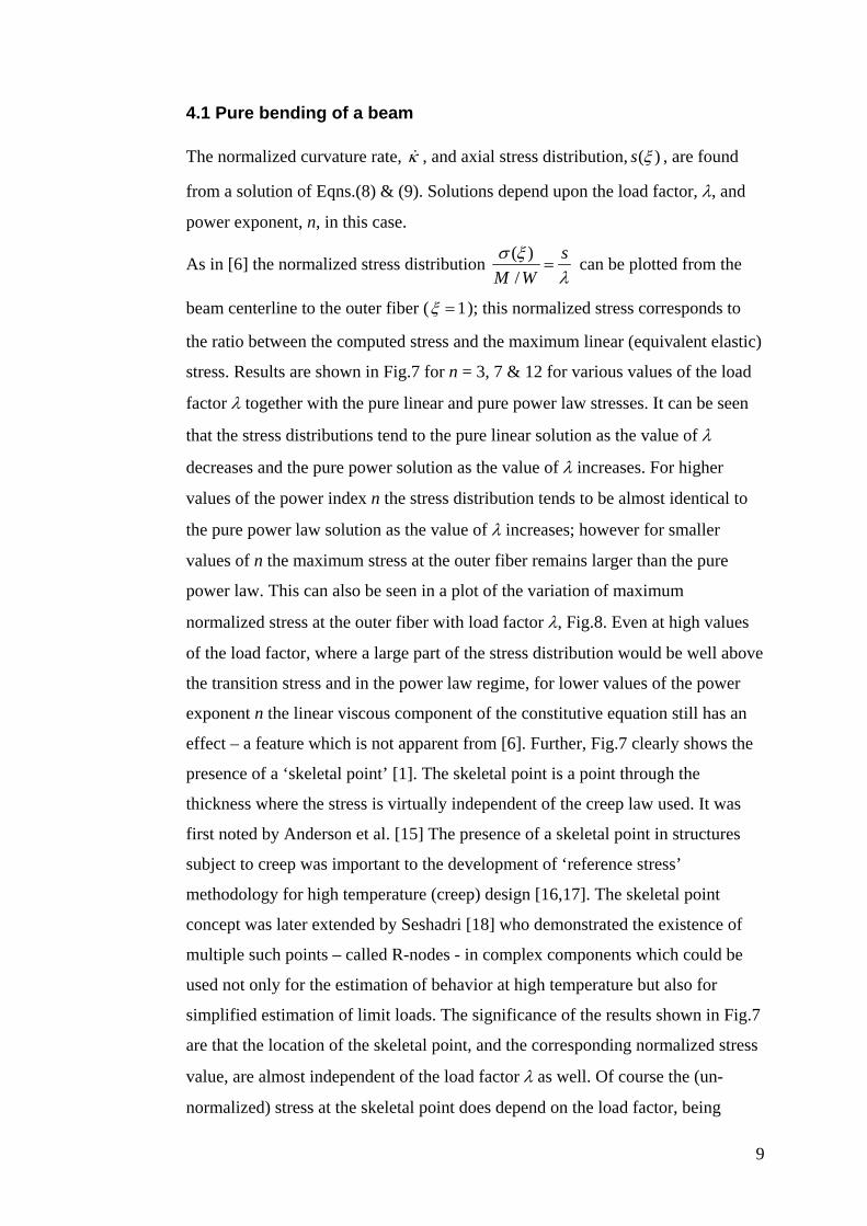
4.1 Pure bending of a beam
The normalized curvature rate, , and axial stress distribution, ( )s , are found
from a solution of Eqns.(8) & (9). Solutions depend upon the load factor, , and
power exponent, n, in this case.
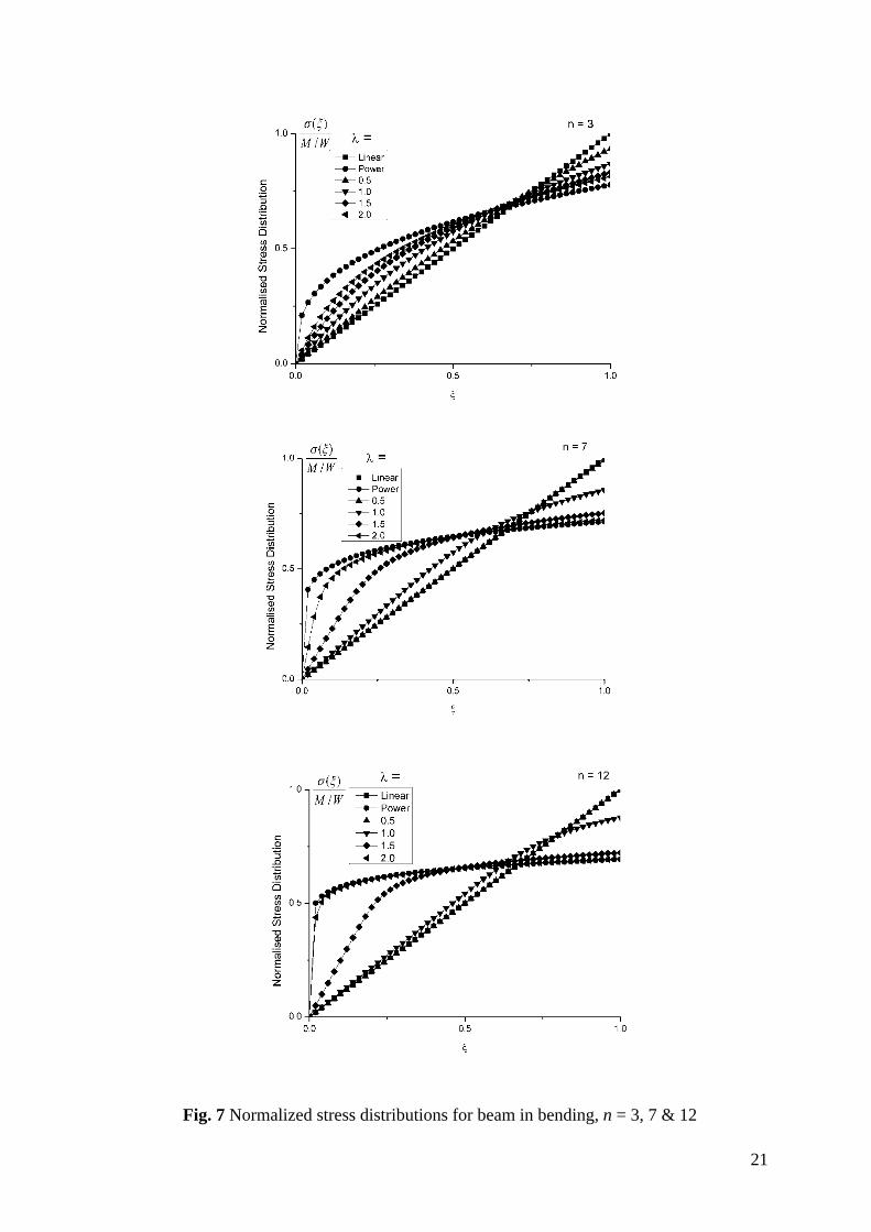
As in [6] the normalized stress distribution ( )
/
s
M W
can be plotted from the
beam centerline to the outer fiber ( 1 ); this normalized stress corresponds to
the ratio between the computed stress and the maximum linear (equivalent elastic)
stress. Results are shown in Fig.7 for n = 3, 7 & 12 for various values of the load
factor together with the pure linear and pure power law stresses. It can be seen
that the stress distributions tend to the pure linear solution as the value of
decreases and the pure power solution as the value of increases. For higher
values of the power index n the stress distribution tends to be almost identical to
the pure power law solution as the value of increases; however for smaller
values of n the maximum stress at the outer fiber remains larger than the pure
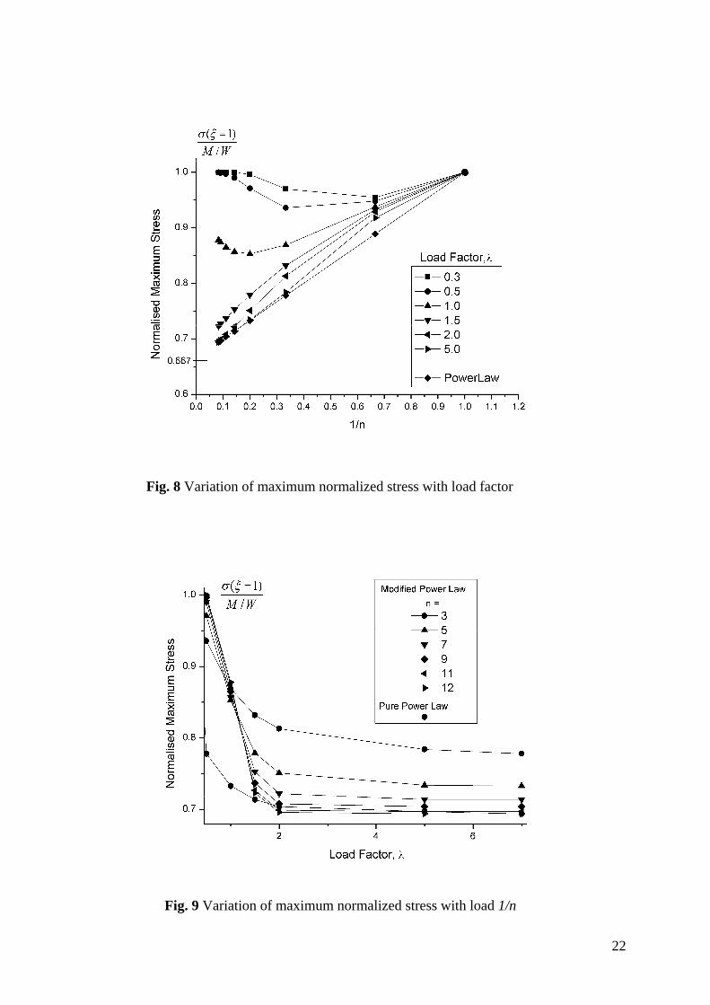
power law. This can also be seen in a plot of the variation of maximum
normalized stress at the outer fiber with load factor , Fig.8. Even at high values
of the load factor, where a large part of the stress distribution would be well above
the transition stress and in the power law regime, for lower values of the power
exponent n the linear viscous component of the constitutive equation still has an
effect – a feature which is not apparent from [6]. Further, Fig.7 clearly shows the
presence of a ‘skeletal point’ [1]. The skeletal point is a point through the
thickness where the stress is virtually independent of the creep law used. It was
first noted by Anderson et al. [15] The presence of a skeletal point in structures
subject to creep was important to the development of ‘reference stress’
methodology for high temperature (creep) design [16,17]. The skeletal point
concept was later extended by Seshadri [18] who demonstrated the existence of
multiple such points – called R-nodes - in complex components which could be
used not only for the estimation of behavior at high temperature but also for
simplified estimation of limit loads. The significance of the results shown in Fig.7
are that the location of the skeletal point, and the corresponding normalized stress
value, are almost independent of the load factor as well. Of course the (un-
normalized) stress at the skeletal point does depend on the load factor, being

10
proportional to the applied load. The skeletal point could be seen in the results
reported in [6] but its significance was not noted.
Further, in pure power law creep it has been observed that the maximum stress in
a component typically exhibits a linear variation with the reciprocal of the power
exponent, n, [1, 19]. For the beam in bending, the maximum normalized stress at
the outer fiber, is exactly obtained as
max 2 1
/ 3M W n
in which the linear variation with 1/n is evident. The limiting values of n =1 and
ncan be shown to correspond to linear elastic and perfectly-plastic
maximum stress. This feature of the pure power law has been demonstrated for
many components and load conditions [1] (a recent example is the peak stress in
an oval pressurized pipe bend [20]). Fig.9 plots the variation of maximum
normalized stress with 1/n for various values of the load factor for the modified
power law. It can be seen that provided the load factor 1 the normalized
maximum stress decreases from n = 1 as 1/n decreases towards n . The
variation tends towards linear with 1/n as the load factor increases. The following
may also be observed if 1 : (a) in all cases as 1n the normalized maximum
stress tends to 1, (b) in all cases as n the maximum stress (seems to) tend to
a value of 2/3, as the pure power law. As a consequence it may be concluded that,
to a good (engineering) approximation, above a certain value of load factor the
maximum stress variation with power exponent using a modified power law can
be well approximated by the pure power law solution, which itself can be well
estimated from linear elastic and perfectly plastic solutions.
The study reported in [6] did not consider the deformation characteristics of the
modified power law. Here the behavior of the normalized curvature rate will be
examined in more detail. Plots of normalized curvature rate, , against the load
factor, , for various values of the power exponent n are shown in Fig.10 – part
(a) shows the complete set of plots for the range of variables studied, while part
(b) focuses on a smaller region using a log/log plot. Fig.11 shows the equivalent
pure power law solution

11
2 1
3
nn
n
for comparison. It can be seen that for values of the load factor less than a ‘cross-
over’ point just less than 1.5 the variation of curvature rate with load factor is
almost linear and the linear viscous part of the constitutive equation dominates.
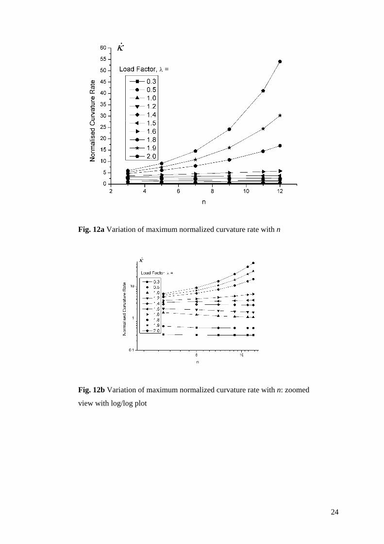
This behavior can be further seen in Fig. 12 where curvature rate is plotted against
the power index n for various values of the load factor - part (a) shows the
complete set of plots for the range of variables studied, while part (b) focuses on a
smaller region with a log/log plot. It can be seen that for 1.5 the curvature rate
is almost independent of the power index n. This feature is perhaps curious since
the stress distributions for such values of load factor are different from the
equivalent linear distributions and the normalized longitudinal strain rate is
proportional to the curvature rate, e . This observation prompted an
examination of the relation between the curvature rates (and therefore also strain
rates) from the pure linear, pure power law and modified power law constitutive
relations. It turns out that, depending on the load factor, deformations using the
modified power law can be reasonably estimated by simply adding the
deformations from pure linear and pure power law in this example. If the load
factor is close to (and less than) the ‘cross-over’ value for the load factor from
Fig.10 then this simple estimation can underestimate by up to 20% for large
values of the power exponent n, but is much less otherwise as shown in Fig.13.
This is an attractive observation: variations in strain rate predictions due to creep
testing, scatter and curve fitting can have similar error levels and the implication
(at least in this simple example) is that deformation rates for a material modeled
by the modified power law could simply be obtained from superimposing
equivalent linear deformations and pure power law creep deformations. The latter
could be estimated for design purposes using reference stress or other robust
simplified methods,. (High temperature creep design rules are more typically
based on deformation rather than stress in the first instance).

12
4.2 Pressurized thick cylinder
The simple thick cylinder problem allows a study of creep under a multi-axial
stress state. For a modified power law, the solution of Eqns. (14), (15) & (16)
depends not only on the power index n and load factor as for the beam in
bending, but also on a geometry factor - the radius ratio . The cylinder geometry
can therefore be varied from moderately-thin to thick: in this study varies takes
values of 1.3, 2.0 and 3.0. In the following study only the circumferential (hoop)
stress will be considered; the radial stress, due to the nature of the boundary
conditions, Eqns. (10), varies in a simple fashion from –p to zero. As a basis for
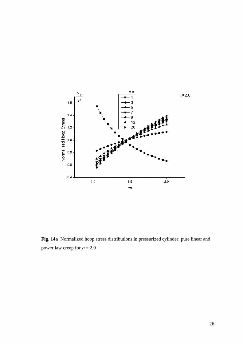
comparison, Figs. 14 (a) shows an example of the hoop stress distribution,
/ p , corresponding to a pure power law, for various values of the power index
n, and to a linear viscous law (n = 1) from Eqns.(17) for = 2.0. This plot can be
used toform the basis of comparisons of stress distribution changes due to the
effect of using the modified power law, where the load factor must be taken into
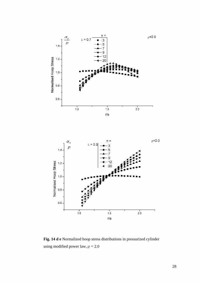
consideration. As is well known, the hoop stress variation through the thickness of
the cylinder in all three cases changes from the pure linear case, where the
maximum stress is at the inside surface, to the pure steady state, where the
maximum stress is at the outside, as can be seen from Fig. 14(a) These limiting
cases then may be compared to the hoop stress distributions as the load factor
varies from 0.2, 0.7, 0.9 & 2.0; these are not reproduced in full here but can be
found in Online Resource 1. Examining each of the plots of Online Resource 1 it
can be seen that as the load factor increases the hoop stress distribution changes
from a form similar to pure linear to that of the pure power law. For the
moderately thick cylinder ( = 1.3) the change occurs between load factors 0.2 &
0.7, Fig. 14 (b) & (c), while for the two thick cylinders ( = 2.0 & 3.0) the change
occurs between load factors 0.7 & 0.9, Fig 14(d) & (e), and 0.9 & 2.0
respectively. More detailed studies show that for the case = 3.0 the change
occurs between load factor 0.9 & 1.3. It is clear then (this was perhaps not
immediately clear from [6]) that the influence of the linear component of the
modified power law is more evident as the thickness increases in the sense that the
power law component does not dominate until higher values of the load factor.
This reflects the fact that the overall stress magnitude reduces as the thickness
increases. Further, as in the case of the beam in bending, an approximate ‘skeletal

13
point’ can be observed: the position of this point moves outwards as the cylinder
thickness increases while the magnitude of the stress at this point decreases. Close
to the values of load factor at which the behavior changes from being more
dominated by the power law component than the linear component of the
modified power law the skeletal point is perhaps less distinct, but arguably the
trend is clear enough for engineering design purposes, as discussed for the beam
in bending. In fact if the von-Mises equivalent stress / p is plotted instead, the
skeletal point becomes more distinct. Finally, as in the case of the beam in
bending, the position of the skeletal point and magnitude of the corresponding
normalized stress value are again almost independent of the load factor with the
(un-normalized) stress being proportional to the applied pressure at the skeletal
point.
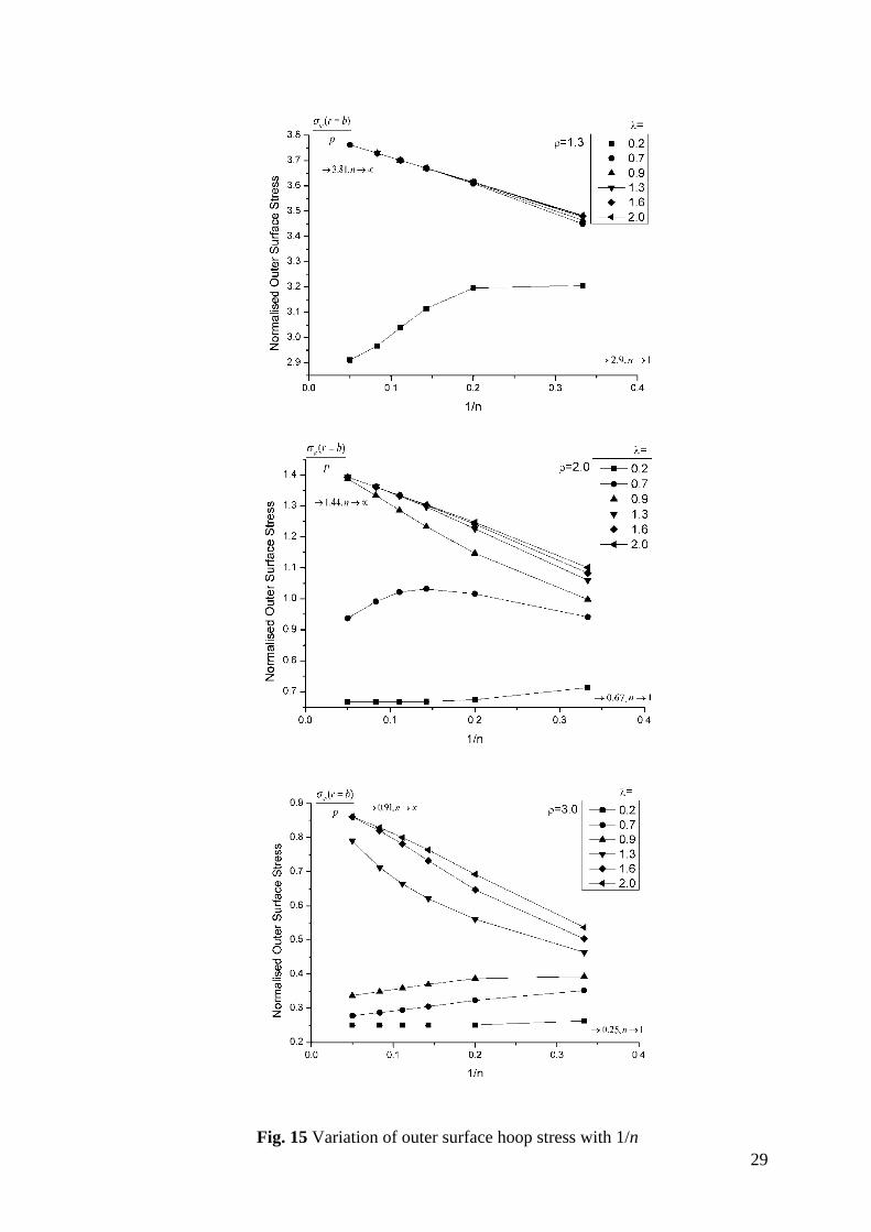
The study of the beam in bending in Sec. 4.1 showed that the maximum stress
exhibited an almost linear variation with the reciprocal of the power index, 1/n.
This observation would need more careful interpretation for the thick cylinder
since, as discussed from Fig. 14, the position of the maximum hoop stress changes
from the inner to the outer surface when considering pure linear and pure power
law. Fig.15 plots the (normalized) outer surface stress as a function of 1/n (with n
in the range 3 to 20) for various values of the load factor and for = 1.3, 2.0 &
3.0. It can be seen that in each case, above some transition value of the load
factor, the outer stress is indeed sensibly linear with 1/n. The limiting values of
the classical pure linear 1n and pure power law nare also indicated on
Fig.15 and it is apparent that the calculated results for the modified power law,
again above some transition value of the load factor, do tend to these limiting
values.
Finally, as for the beam in bending, the study reported in [6] did not consider the
deformation characteristics for the thick cylinder. The normalized maximum
displacement at the inside surface, Eqn.(16), is plotted in Fig.16 against the load
factor for various values of n - a log-log scale is used for discussion purposes.
Three values of thickness are used as before and in each case, similar to the beam
in bending, there is a cross-over value of load factor below which the variation of
maximum displacement is almost linear with respect to the load factor (this can be
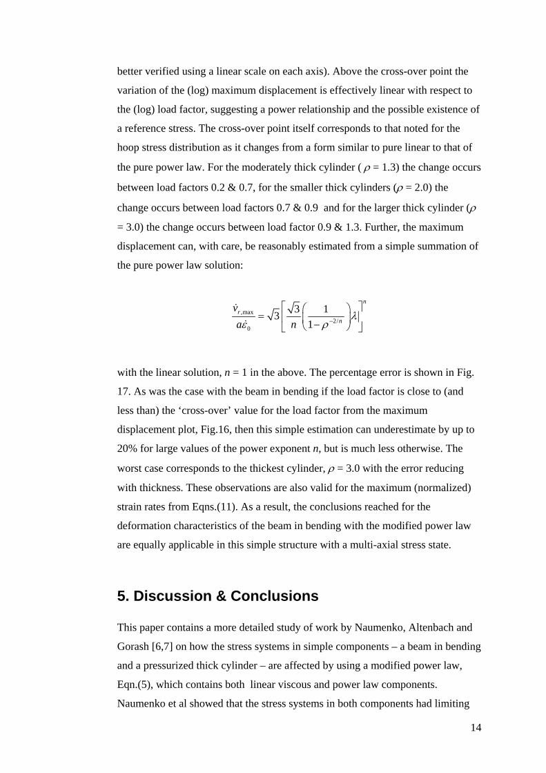
14
better verified using a linear scale on each axis). Above the cross-over point the
variation of the (log) maximum displacement is effectively linear with respect to
the (log) load factor, suggesting a power relationship and the possible existence of
a reference stress. The cross-over point itself corresponds to that noted for the
hoop stress distribution as it changes from a form similar to pure linear to that of
the pure power law. For the moderately thick cylinder ( = 1.3) the change occurs
between load factors 0.2 & 0.7, for the smaller thick cylinders ( = 2.0) the
change occurs between load factors 0.7 & 0.9 and for the larger thick cylinder (
= 3.0) the change occurs between load factor 0.9 & 1.3. Further, the maximum
displacement can, with care, be reasonably estimated from a simple summation of
the pure power law solution:
,max
2/0
3 13
1
n
r
n
v
a n
with the linear solution, n = 1 in the above. The percentage error is shown in Fig.
17. As was the case with the beam in bending if the load factor is close to (and
less than) the ‘cross-over’ value for the load factor from the maximum
displacement plot, Fig.16, then this simple estimation can underestimate by up to
20% for large values of the power exponent n, but is much less otherwise. The
worst case corresponds to the thickest cylinder, = 3.0 with the error reducing
with thickness. These observations are also valid for the maximum (normalized)
strain rates from Eqns.(11). As a result, the conclusions reached for the
deformation characteristics of the beam in bending with the modified power law
are equally applicable in this simple structure with a multi-axial stress state.
5. Discussion & Conclusions
This paper contains a more detailed study of work by Naumenko, Altenbach and
Gorash [6,7] on how the stress systems in simple components – a beam in bending
and a pressurized thick cylinder – are affected by using a modified power law,
Eqn.(5), which contains both linear viscous and power law components.
Naumenko et al showed that the stress systems in both components had limiting

15
cases for low and high stress, namely the pure viscous and pure power law
respectively. Between these limiting cases the (normalized) stress distributions
depended not only on the exponent in the power law, but also some load factor
since the modified power law solutions cannot be normalized to eliminate applied
load. In this study the analysis has been extended to examine the role of simplified
methods for estimating stress for design purposes and also to investigate the effect
of the modified power law on deformation rates.
It is clear that the stress distributions for the beam in bending, Fig.7, and thick
cylinder, Fig.14, change considerably from the limiting cases of pure linear
viscous and pure power law, especially as the respective load factor changes,
especially close to the transition from linear dominance to power law dominance.
Nevertheless some characteristic features of the stress distributions found for pure
power law can still be seen in both components: (i) the presence of a skeletal point
[15,16], where the normalized stress value is almost independent of the exponent
in the power law and also the load factor, and (ii) above some transition load
factor the maximum stress is approximately linear with respect to the reciprocal of
the power exponent, 1/n, with the limiting cases of 1n and n remaining
the linear viscous solution and perfectly plastic solutions respectively, as in the
case of the pure power law [19]. The latter seems to be valid even though large
parts of the component continue to be dominated by the linear component,
although the maximum stress location is dominated by the power law component.
It has also been demonstrated that the maximum displacement and strain rates in
these two components can be sensibly estimated through a superposition of the
pure linear and pure power law solutions, except for load factors close to the
transition from linear to power law dominance coupled with high values of the
power exponent, n, Figs 13 & 17. The worst estimates are no more than 20%
lower than the true solution and for a fairly wide range of load factor no more
than 10% - this being well within currently acceptable bounds for scatter in creep
data. There is the clear implication that maximum deformation rates can be
reasonably estimated (as a lower bound in both examples) from superposition of
linear and power law solutions, the latter allowing simplified estimates using
reference stress, linear elastic and perfectly plastic limit solutions [1-3].

16
In conclusion, it is apparent that the simple robust methods developed for the
estimation of maximum stress and deformation rate of components subject to pure
power law creep [1-3] continue to have some relevance for the modified power
law. Further work in the area of steady creep therefore includes a verification of
these results for more complex structures using detailed finite element analysis
and a more detailed study of the range of applicability of the simplified methods.
Indeed, this study has only considered steady creep under constant load and gives
no consideration of relaxation and redistribution of stress. Naumenko et al [6]
briefly examined relaxation of a bar using the modified creep law, demonstrating
that a stress range dependent creep law could have significant effect. That
example has been extended by the author [14] to more complex structures
undergoing creep relaxation, in particular elastic follow-up: it is shown there that
a stress range dependent creep law wholly alters the time dependent structural
response, unlike the steady creep cases described herein where familiar features
are retained.
References
1. Boyle, J.T., Spence, J.: Stress Analysis for Creep. Butterworths, London (1983)
2. Penny, R.K., Marriott, D.L.: Design for Creep. Chapman & Hall, London (1995)
3. Kraus, H.: Creep Analysis. Wiley, New York (1980)
4. Wilshire, B.: Observations, theories and predictions of high temperature creep behavior. Mettal.
& Mater. Trans. 33A:241-248 (2002)
5. Frost, H.J., Ashby, M.F.: Deformation-Mechanism Maps. Pergamon, Oxford (1982)
6. Naumenko, K., Altenbach, H., Gorash, Y.: Creep analysis with a stress range dependent
constitutive model. Arch. Appl. Mech. 79:619-630 (2009)
7. Altenbach, H., Gorash, Y., Naumenko, K.: Steady-state creep of a pressurized thick cylinder in
both the linear and power law ranges. Acta. Mech. 196:263-274 (2008)
8. Altenbach, H., Naumenko, K.,Gorash Y.: creep analysis for a wide stress range based on stress
relaxation experiments. Int. J. Modern Physics 22B:5413-5418 (2008)
9. Reith, M. et al: Creep of the Austenitic Steel AISI 316 L(N). Forschungszentrum Karlsruhe in
der Helmholtz-Gemeinschaft, Wissenschaftliche Berichte FZKA 7065 (2004)
10. Evans, R.W., Parker J.D., Wilshire B.: In: Wilshire B., Owen D.R.J. (eds.) Recent Advances in
Creep and Fracture of Engineering Materials and Structures; 135-184 (1982)
11. Garofalo, F.: An empirical relation defining the stress dependence of minimum creep rate in
metals. Trans. the Metall . Soc. AIME 227:351-356 (1963)

17
12. Naumenko, K., Altenbach, H.: Modelling of Creep for Structural Analysis. Springer, Berlin
(2007)
13. Williams, K. R., Wilshire, B.: On the Stress- and Temperature-Dependence of Creep of
Nimonic 80A. Met. Sci. J. 7:176-179 (1973)
14. Boyle, J.T.: Stress relaxation and elastic follow-up using a stress range dependent constitutive
model (Submitted)
15. Anderson, R.G. et al: Deformation of uniformly loaded beams obeying complex creep laws.
Journ. Mech. Eng. Sci. 5:238-244 (1963)
16. Anderson, R. G.: Some observations on reference stresses, skeletal points, limit loads and
finite elements. In: Creep in Structures, 3rd IUTAM Symposium, Leicester 166-178 (1981)
17. Boyle, J.T., Seshadri R.: The reference stress method in creep design: a thirty year
retrospective. General Lecture, In: Proc IUTAM Symposium on Creep in Structures, Nagoya, Ed.
S Murakami & N Ohno, 297-311, Kluwer (2000)
18. Seshadri, R.: Inelastic evaluation of mechanical and structural components
using the generalized local stress strain method of analysis. Nuclear Engineering and Design
153:287-303 (1995)
19. Calladine, C.R.: A rapid method for estimating the greatest stress in a structure subject to
creep. Proc. IMechE. Conf. Thermal Loading and Creep (1964)
20. Yaghi, A.H.,Hyde, T.H., Becker, A.A., Sun, W.: Parametric peak stress functions of 90 pipe
bends with ovality under steady-state creep conditions. Int. Journ. Press. Vess. Piping 86:684-692
(2009)

18
Fig. 1 Steady creep of austenitic AISI 316 L(N) 550-650C after [9]
Fig. 2 Steady creep of 0.5Cr0.5Mo0.25V after [4]

19
Fig. 4 Steady creep 9%Cr steel at 600C after [6]
Fig. 3 Steady creep of austenitic AISI 316 L(N) 550-750C after [9]

20
Fig. 5 Geometry and loading of a beam with rectangular cross section
Fig. 6 Geometry and loading of a pressurized thick cylinder
21
Fig. 7 Normalized stress distributions for beam in bending, n = 3, 7 & 12
22
Fig. 8 Variation of maximum normalized stress with load factor
Fig. 9 Variation of maximum normalized stress with load 1/n

23
Fig. 10a Variation of maximum normalized curvature rate with load factor
Fig. 10b Variation of maximum normalized curvature rate with load factor: zoomed view with log/log plot
Fig. 11 Variation of maximum normalized curvature rate with load factor: pure power law creep
24
Fig. 12a Variation of maximum normalized curvature rate with n
Fig. 12b Variation of maximum normalized curvature rate with n: zoomed
view with log/log plot

25
Fig. 13 Percentage error in normalized curvature rate comparing modified
power law and superposition of pure linear and pure power law
26
Fig. 14a Normalized hoop stress distributions in pressurized cylinder: pure linear and
power law creep for = 2.0

27
Fig. 14 b c Normalized hoop stress distributions in pressurized cylinder
using modified power law, = 1.3
28
Fig. 14 d e Normalized hoop stress distributions in pressurized cylinder
using modified power law, = 2.0
29
Fig. 15 Variation of outer surface hoop stress with 1/n

30
Fig. 16 Variation of maximum normalized displacement with load factor

31
Fig. 17 Percentage error in maximum normalized displacement comparing
modified power law and superposition of pure linear and pure power law
Recommended