Psicologica (2012), 33, 362-390.
The Dirichlet-Multinomial Model for Multivariate
Randomized Response Data and Small Samples
Marianna Avetisyan∗ & Jean-Paul Fox
University of Twente, the Netherlands
In survey sampling the randomized response (RR) technique can
be used to obtain truthful answers to sensitive questions. Although
the individual answers are masked due to the RR technique, individual
(sensitive) response rates can be estimated when observing multivariate
response data. The beta-binomial model for binary RR data will be
generalized to handle multivariate categorical RR data. The Dirichlet-
multinomial model for categorical RR data is extended with a linear
transformation of the masked individual categorical-response rates to
correct for the RR design and to retrieve the sensitive categorical-response
rates even for small data samples. This specification of the Dirichlet-
multinomial model enables a straightforward empirical Bayes estimation of
the model parameters. A constrained-Dirichlet prior will be introduced to
identify homogeneity restrictions in response rates across persons and/or
categories. The performance of the full Bayes parameter estimation
method is verified using simulated data. The proposed model will be
applied to the college alcohol problem scale study, where students were
interviewed directly or interviewed via the randomized response technique
about negative consequences from drinking.
The data collection through surveys based on direct-questioning methods
has been the most common way. The direct-questioning techniques
are usually assumed to provide the necessary level of reliability when
measuring opinions, attitudes, and behaviors. However, individuals with
different types of response behavior who are confronted with items about
sensitive issues of human life regarding ethical (stigmatizing) and legal
(prosecution) implications are reluctant to supply truthful answers.
∗E-mail: [email protected]
Dirichlet-multinomial model for RR data 363
Tourangeau, Rips, and Rasinski (2000), and Tourangeau and Yan (2007)
argued that socially desirable answers and refusals are to be expected when
asking sensitive questions directly.
Warner (1965), and Greenberg, Abu-Ela, Simmons, and Horvitz
(1969) developed RR techniques to obtain truthful answers to sensitive
questions in such a way that the individual answers are protected but
population characteristics can be estimated. These techniques are based on
univariate RR data. Recently, RR models have been developed to analyze
multivariate response data, where the item responses are nested within
the individual. Although the individual answers are masked due to the
RR technique, individual (sensitive) characteristics can be estimated when
observing multivariate RR data. Fox (2005) and Bockenholt and van der
Heijden (2007) introduced item response models for binary RR data. The
applications are focusing on surveys where the items measure an underlying
sensitive construct. The so-called randomized item response models have
been extended to handle categorical RR data by Fox and Wyrick (2008)
and De Jong, Pieters, and Fox (2010). The class of randomized item
response models are meant for large-scale survey data, since person as
well as item parameters need to be estimated (Fox and Wyrick, 2008). For
categorical item response data, more than 500 respondents are often needed
to obtain stable parameter estimates. Furthermore, the randomized item
response data are less informative than the direct-questioning data, since the
RR technique engenders additional random noise to the data. Fox (2008)
proposed a beta-binomial model for analyzing multivariate binary RR data,
which enables the computation of individual response estimates without
requiring a large-scale data set. The beta-binomial model has several
advantages like a simple interpretation of the model parameters, stable
parameter estimates for relatively small data sets, and a straightforward
empirical Bayes estimation method.
Here, a Dirichlet-multinomial model is proposed for handling
multivariate categorical RR data such that individual category-response
rates can be estimated. The individual observed RR data consist of a
number of randomized responses per category. Each individual set of
observed numbers are assumed to be multinomially distributed given the
individual category-response rates. The individual category-response rates
are assumed to follow a Dirichlet distribution. The individual response rates
are related to the observed randomized responses, which make them not
useful for the inferences basing on regular statistical approaches. However,
364 M. Avetisyan & J.-P. Fox
it will be shown that the individual category-response rates are linearly
related to the model-based (true) category-response rates. The latter one
relates to the latent responses, which are expected under the model when
the responses are not masked due to the randomized response technique.
The parameters of the linear transformation are design parameters and
are known characteristics of the randomizing device that is used to
mask the individual answers. The transformed categorical-response rates
will provide information about the latent individual characteristic that is
measured by the survey items. Analytical expressions of the posterior mean
and standard deviation of the true individual categorical-response rates will
be given. The expressions can be used for estimation given prior knowledge
or empirical Bayes estimates of the population response rates. Furthermore,
a WinBUGS implementation is given for a full Bayes estimation of the
model parameters.
To model and to identify constraints of homogeneity in category-
response rates, the restricted-Dirichlet prior (Schafer, 1997) is used. The
restriction on the Dirichlet prior can be used to identify effects of the
randomized response mechanism across individuals, groups of individuals,
and response categories.
In the next section, the randomized response technique is described
in a multiple-item setting. The beta-binomial model is described for
multivariate binary RR outcomes. Then, as a generalization, the Dirichlet-
multinomial model is presented for multivariate categorical RR data.
Properties of the conditional posterior distribution of the true individual
categorical-response rates are derived given observed randomized response
data. Then, empirical and full Bayes methods are proposed to estimate
all model parameters. A simulation study is given, where the properties
of the estimation methods are examined. Finally, the model will be used
to analyze data from a college alcohol problem scale survey, where U.S.
college students were asked about their alcohol drinking behavior with and
without using the randomized response technique. The restricted-Dirichlet
prior will be used to test assumptions of homogeneity over persons and
response categories. In particular, it will be shown that the effect of the
RR method varies over response categories, where the RR effect will be the
highest for the most sensitive response option.
Dirichlet-multinomial model for RR data 365
MULTIVARIATE RANDOMIZED RESPONSETECHNIQUES
In Warner’s RR technique (Warner, 1965) for univariate binary response
data, in the data collection procedure a randomizing device (RD) is
introduced. For each respondent the RD directs the choice of one of
two logically opposite questions. This sampling design guarantees the
confidentiality of the individual answers, since they cannot be related
directly to one of the opposite questions.
Greenberg et al. (1969) proposed the unrelated question technique,
where the outcome of the RD refers to the study-related sensitive question
or an irrelevant unrelated question. The RD is specified in such a way
that the sensitive question is selected with probability φ1 and the unrelated
question with probability 1− φ1. This RR method is extended to a forced
response method (Edgell, Himmelfarb, and Duchan, 1982), where the
unrelated question is not specified but an additional RD is used to generate
a forced answer. Each observed individual answer is protected, since it
cannot be revealed whether it is a true answer to the sensitive question or a
forced answer generated by the RD. As a result, the observed RR answers
are polluted by forced responses.
Let RD = 1 denote the event that an answer to the sensitive question is
required and P(RD = 1) = φ1k and RD = 0 otherwise. A forced positive
response to item k is generated with probability φ2k. For a multiple-item
survey, the probability of a positive RR of respondent i, given a forced
response sampling design, can be stated as
P(Yik = 1 | φ, pik) = P(RD = 1)pik +(1−P(RD = 1))φ2k, (1)
where the true response rate of person i to item k is denoted as pik. Note
that the response model for the RR data is a two-component mixture model.
For the first component the sensitive question needs to be answered and
for the second component a forced response needs to be generated. Thus,
the randomized response probability equals the true or the forced response
probability depending on the RD outcome. With φ1k > 1/2, for all k,
the data contain sufficient information to make inferences about the true
response rates.
The multiple items will be assumed to measure an underlying individual
response rate (e.g., alcohol dependence, academic fraud) such that pik =pi for all k. This individual response rate can be estimated from
366 M. Avetisyan & J.-P. Fox
the multivariate RR data. Note that in a multivariate setting the RD
characteristics are allowed to vary over items such that the proportion
of forced responses can vary over items. In practice, the sensitivity
of the items may vary although they relate to the same sensitive latent
characteristic. This variation in sensitivity can be controlled by adjusting
the RD characteristics, which are under the control of the interviewer.
The forced response model in Equation (1) can be extended to handle
polytomous multivariate RR data. Let φ2k(c) denote the probability of
a forced response in category c for c = 1, . . . ,Ck such that the number
of response categories may vary over items. The categorical-response
rates of individual i are denoted as pi(1), . . . , pi(Ck), which represent
the probabilities of honest (true) responses corresponding to the response
categories of item k. The probability of an observed randomized response
of individual i in category c of item k can be stated as,
P(Yik = c | φ, pik) = φ1k pi(c)+(1−φ1k)φ2k(c). (2)
This forced RR model for categorical data can be used to measure
individual categorical response rates related to a sensitive characteristic.
The individual answers are not known but the multivariate data make it
possible to retrieve information about latent individual characteristics.
THE BETA-BINOMIAL MODEL FOR MULTIVARIATEBINARY RR DATA
Let each participant i = 1, . . . ,N respond to k = 1, . . . ,K binary items. The
observations ui1, . . . ,uiK represent the answers of the ith participant to the K
items. The response observations are assumed to be Bernoulli distributed
given response rate pi for individual i. The observations are assumed to be
independently distributed given the response rate. Therefore, the sum of
individual response observations is binomially distributed with parameters
K and pi.
It is to be expected that the response rates vary over participants. This
variation is modeled by means of a beta distribution with parameters αand β, which specify the distribution of the response rates. This leads
to the following hierarchical model for the multivariate binary response

Dirichlet-multinomial model for RR data 367
observations,
Ui· | pi ∼ BI N (K, pi),
pi | α, β ∼ B(α, β),
where Ui· = ∑k Uik.
Within a Bayesian modeling approach, the beta prior distribution for
parameter pi is a conjugated prior when the data are binomially distributed
given the response rate. In that case, the posterior distribution of the
response rate is also a beta distribution. That is,
p(
pi | ui·, α, β)
=f (ui· | pi)π(pi | α, β)∫
f (ui· | pi)π(pi | α, β)d pi
=Γ(K + α+ β)
Γ(ui·+ α)Γ(K −ui·+ β)pui·+α−1
i (1− pi)K−ui·+β−1,
which can be recognized as a beta density with parameters ui·+ α and K −ui·+ β. The posterior mean and the variance are
E(pi | ui· , α, β) =ui· + α
K + α+ β,
Var(pi | ui· , α, β) =(ui· + α)(K −ui· + β)
(K + α+ β+1)(K + α+ β)2,
respectively. It follows that posterior inferences can be directly made when
knowing the population parameters α and β.
In a forced response design, the observations u are masked and
randomized responses y are observed. The RD specifies the probabilities
governing this randomization process such that an honest response is
to be given with probability φ1 and a positive forced response with
probability (1− φ1)φ2. The probability of observing a positive response
from participant i to item k is related to the true response by the following
expression:
P(Yik = 1 | pi) = φ1 f (uik | pi)+(1−φ1)φ2
= φ1 pi +(1−φ1)φ2 = Δ(pi).
368 M. Avetisyan & J.-P. Fox
It can be seen that the forced response design corresponds with a linear
transformation of the response rate. This linear transformation function,
Δ(.), operates on the individual response rate of the true responses.
Therefore, the beta-binomial model accommodates the forced response
sampling mechanism by modeling the linearly transformed response rates;
that is,
Yi· | pi ∼ BI N (K,Δ(pi)) ,Δ(pi) ∼ B(α,β),
where the transformation parameters φ1 and φ2 are characteristics of the RD
and are known a priori.
A population distribution is specified for the transformed response rates.
The transformed response rates are a priori beta distributed, which is the
conjugated prior for the binomially distributed likelihood. As a result, the
posterior distribution of the transformed response rates is beta distributed
with parameters yi·+α and K − yi·+β.
The posterior expected response rate given the randomized responses
can be expressed as
E (Δ(pi) | yi· ,α,β) =yi· +α
K +α+β= Δ(E(pi) | yi· ,α,β)
= φ1E (pi | yi· ,α,β)+(1−φ1)φ2,
using that the expected value of the linearly transformed response rate
equals the linearly transformed expected response rate. As a result, the
posterior expected value of the (true) response rate can be expressed as
E (pi | yi· ,α,β) = φ−11
(yi· +α
K +α+β
)+(1−φ−1
1 )φ2. (3)
In the same way, an expression can be found for the posterior variance of
the true response rate,
Var (pi | yi· ,α,β) =(yi· +α)(K − yi· +β)
φ21(K +α+β+1)(K +α+β)2
.
There are two straightforward methods for estimating the hyperparameters
α and β, the method of moments and the method of maximizing the
marginal likelihood. Given the estimated hyperparameters, empirical

Dirichlet-multinomial model for RR data 369
Bayes estimates of the response rates can be derived by inserting the
hyperparameter estimates into Equation (3). Furthermore, the estimation
of confidence intervals and Bayes factors is described in Fox (2008).
THE DIRICHLET-MULTINOMIAL MODEL FORMULTIVARIATE CATEGORICAL RR DATA
The number of responses per response category over items for person
i are stored in a vector ui· = (ui·1, . . . ,ui·C)t , where ui·c = ∑k uikc for c =
1, . . . ,C. They represent the number of choices per response category
over items. In the college alcohol study we will present in Section 7.2,
the data represent the frequency of alcohol-related negative consequences.
In marketing research, Goodhardt, Ehrenberg, and Chatfield (1984)
considered data about individual number of purchases per brand in a time
period. In social research, Wilson and Chen (2007) considered frequencies
to television viewing questions from the High School and Beyond survey
study in the United States. Their item-based test is assumed to measure
the daily television viewing habit and interest is focused on time-specific
population response rates.
The number of responses per category given the category response rates
are assumed to be independently distributed. They can be modeled by
a multinomial distribution with parameters K and category response rates
pi1, . . . , piC. For respondent i, the contribution to the likelihood is
f (ui· | pi) =K!
∏c ui·c! ∏c
pui·cic .
The variability in the vectors of response counts is often higher than can
be accommodated by the multinomial distribution. Therefore, individual
variation in category response rates is modeled by a Dirichlet distribution
with parameters α = (α1, . . . , αC), which is represented by
π(pi | α) =Γ(α0)
∏c Γ(αc)∏
cpαc−1
ic .
where α0 =∑c αc. The within-individual and between-individual variability
370 M. Avetisyan & J.-P. Fox
in response rates is described by a Dirichlet-multinomial model; that is,
Ui·1, . . . ,Ui·C | pi1, . . . , piC ∼ Mult(K, pi1, . . . , piC),pi1, . . . , piC ∼ D(α1, . . . , αC),
where Ui·c = ∑k Uikc for c = 1, . . . ,C. The compact form of this expression
can be written in terms of vector notation
Ui· | pi ∼ Mult(K,pi) ,pi ∼ D(α),
where Ui· = (Ui·1, . . . ,Ui·C)t .
The Dirichlet distribution is a conjugate prior for the parameters of the
multinomially distributed responses. Therefore, the conditional posterior
distribution of the category response rates is a Dirichlet distribution, which
is represented by
p(pi | ui· , α) =f (ui· | pi)π(pi | α)∫
f (ui· | pi)π(pi | α)dpi
=Γ(K + α0)
∏c Γ(ui·c + αc)∏
cpui·c+αc−1
ic .
The posterior mean and the variance of the category response rates of
individual i equals
E(pic | ui· , α) =ui·c + αc
K + α0
and
Var(pic | ui· , α) =(ui·c + αc)(K + α0 − (ui·c + αc))
(K + α0 +1)(K + α0)2,
respectively, where the prior parameters α are unknown.
According to Equation (2), the probability of an observed randomized
response in category c for item k can be expressed as
P(Yik = c | pic) = φ1 pic +(1−φ1)φ2(c)= Δ(pic),
where Δ(pic) is the linearly transformed category-response rate of person
Dirichlet-multinomial model for RR data 371
i, which depends on the parameters of the forced randomized response
design. Let yi· = (yi·1, . . . ,yi·C)t denote the vector of observed randomized
count data per response category across items for subject i. The Dirichlet-
multinomial model for the observed randomized count data per category
takes the form
Yi· | pi ∼ Mult(K,Δ(pi)) ,Δ(pi) ∼ D(α), (4)
where Yi· = (Yi·1, . . . ,Yi·C)t and Δ(pi) = (Δ(pi1), . . . ,Δ(piC))
t .
The conditional posterior distribution of the transformed category-
response rate can now be stated as
p(Δ(pi) | yi· ,α) =Γ(K +α0)
∏c Γ(yi·c +αc)∏
c(Δ(pic))
yi·c+αc−1.
Subsequently, the posterior expected (true) category-response rate can be
obtained through a linear transformation. That is,
E (Δ(pic) | yi· ,α) =yi·c +αc
K +α0= Δ(E (pic) | yi· ,α) (5)
= φ1E (pic | yi· ,α)+(1−φ1)φ2(c).
Applying the inverse of the linear transformation on E(Δ(pic) | yi·,α), the
conditional posterior expected value can be obtained as
E(pic | yi· ,α) = φ−11
(yi·c +αc
K +α0
)+(1−φ−1
1 )φ2(c).
The expression for the conditional posterior variance can be derived in a
similar way and is equal to
Var (pic | yi· ,α) =(yi·c +αc)(K +α0 − (yi·c +αc))
φ21 (K +α0 +1)(K +α0)
2.
EMPIRICAL BAYES AND FULL BAYES ESTIMATION
There are two major approaches for estimating the model parameters when
the prior parameters are unknown. An empirical Bayes approach, where the
372 M. Avetisyan & J.-P. Fox
prior parameters are estimated from the marginal likelihood of the data and
a full Bayes approach where hyperpriors are defined for the prior parameters
and all model parameters are estimated simultaneously.
EMPIRICAL BAYES ESTIMATION
The marginal distribution of the data given the prior parameters is obtained
by integrating out the category-response rates. In Appendix A, a derivation
is given of the marginal likelihood of the randomized response data given
the prior parameters α. This conditional distribution is given by
p(y | α) = ∏i
∫Δ(pi)
p(yi· | Δ(pi)) p(Δ(pi) | α)d(Δ(pi))
= ∏i
K!
∏c yi·c!
Γ(α0)
∏c Γ(αc)
∏c Γ(αc + yi·c)
Γ(α0 +K).
There are two ways of obtaining empirical Bayes estimates from this
marginal likelihood. The most straightforward way is using the method
of moments (Brier, 1980; Danaher, 1988; Mosimann, 1962). The second
way is the method of marginal maximum likelihood (Paul, Balasooriya,
and Banerjee, 2005).
Method of Moments. Let the sum of the prior parameters be α0 and the
fraction αcα0
for each c be greater than zero. Now, the observed proportion of
category responses is used to estimate the fraction αcα0
; that is,
N−1N
∑i=1
yi·c/K =αc
α0,
for c = 1, . . . ,C. The sum of the prior parameters α0 is estimated using a
relationship between the covariance matrix of the observed data, denoted as
Σy of dimension (C−1)(C−1), and of the category response rates, denoted
as ΣΔ(p) of dimension (C−1)(C−1). Mosimann (1962) showed that
(1+α0)Σy = (K +α0)ΣΔ(p). (6)
The observed data can be used to estimate the covariance matrices; that is,
Σy =
{(N −1)−1 ∑N
i=1 (yi.c − y..c)2 diagonal terms,
(N −1)−1 ∑Ni=1 (yi.c − y..c)(yi.c′ − y..c′) off-diagonal terms, c �= c′
Dirichlet-multinomial model for RR data 373
and
ΣΔ(p) =
{y..c (K − y..c)/K diagonal terms,−y..cy..c′/K off-diagonal terms, c �= c′,
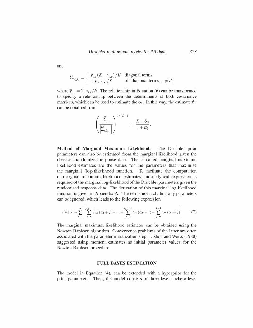
where y..c = ∑i yi.c/N. The relationship in Equation (6) can be transformed
to specify a relationship between the determinants of both covariance
matrices, which can be used to estimate the α0. In this way, the estimate α0
can be obtained from⎛⎝∣∣∣Σy
∣∣∣∣∣∣ΣΔ(p)
∣∣∣⎞⎠1/(C−1)
=K + α0
1+ α0.
Method of Marginal Maximum Likelihood. The Dirichlet prior
parameters can also be estimated from the marginal likelihood given the
observed randomized response data. The so-called marginal maximum
likelihood estimates are the values for the parameters that maximize
the marginal (log-)likelihood function. To facilitate the computation
of marginal maximum likelihood estimates, an analytical expression is
required of the marginal log-likelihood of the Dirichlet parameters given the
randomized response data. The derivation of this marginal log-likelihood
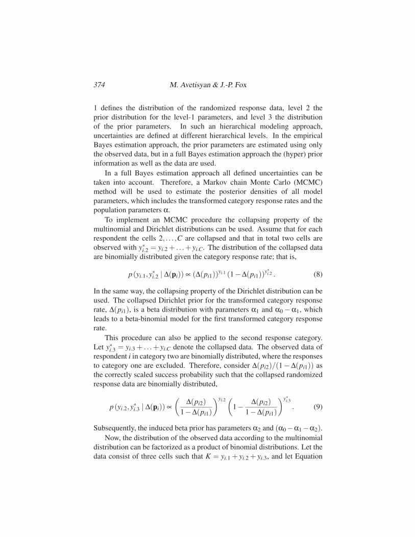
function is given in Appendix A. The terms not including any parameters
can be ignored, which leads to the following expression
l(α | y) ∝N
∑i=1
[yi.1−1
∑j=0
log(α1 + j)+ . . .+yi.C−1
∑j=0
log(αC + j)−K−1
∑j=0
log(α0 + j)
]. (7)
The marginal maximum likelihood estimates can be obtained using the
Newton-Raphson algorithm. Convergence problems of the latter are often
associated with the parameter initialization step. Dishon and Weiss (1980)
suggested using moment estimates as initial parameter values for the
Newton-Raphson procedure.
FULL BAYES ESTIMATION
The model in Equation (4), can be extended with a hyperprior for the
prior parameters. Then, the model consists of three levels, where level
374 M. Avetisyan & J.-P. Fox
1 defines the distribution of the randomized response data, level 2 the
prior distribution for the level-1 parameters, and level 3 the distribution
of the prior parameters. In such an hierarchical modeling approach,
uncertainties are defined at different hierarchical levels. In the empirical
Bayes estimation approach, the prior parameters are estimated using only
the observed data, but in a full Bayes estimation approach the (hyper) prior
information as well as the data are used.
In a full Bayes estimation approach all defined uncertainties can be
taken into account. Therefore, a Markov chain Monte Carlo (MCMC)
method will be used to estimate the posterior densities of all model
parameters, which includes the transformed category response rates and the
population parameters α.
To implement an MCMC procedure the collapsing property of the
multinomial and Dirichlet distributions can be used. Assume that for each
respondent the cells 2, . . . ,C are collapsed and that in total two cells are
observed with y∗i.2 = yi.2 + . . .+ yi.C. The distribution of the collapsed data
are binomially distributed given the category response rate; that is,
p(yi.1,y∗i.2 | Δ(pi)) ∝ (Δ(pi1))yi.1 (1−Δ(pi1))
y∗i.2 . (8)
In the same way, the collapsing property of the Dirichlet distribution can be
used. The collapsed Dirichlet prior for the transformed category response
rate, Δ(pi1), is a beta distribution with parameters α1 and α0 −α1, which
leads to a beta-binomial model for the first transformed category response
rate.
This procedure can also be applied to the second response category.
Let y∗i.3 = yi.3 + . . .+ yi.C denote the collapsed data. The observed data of
respondent i in category two are binomially distributed, where the responses
to category one are excluded. Therefore, consider Δ(pi2)/(1−Δ(pi1)) as
the correctly scaled success probability such that the collapsed randomized
response data are binomially distributed,
p(yi.2,y∗i.3 | Δ(pi)) ∝(
Δ(pi2)
1−Δ(pi1)
)yi.2(
1− Δ(pi2)
1−Δ(pi1)
)y∗i.3. (9)
Subsequently, the induced beta prior has parameters α2 and (α0−α1−α2).
Now, the distribution of the observed data according to the multinomial
distribution can be factorized as a product of binomial distributions. Let the
data consist of three cells such that K = yi.1 + yi.2 + yi.3, and let Equation
Dirichlet-multinomial model for RR data 375
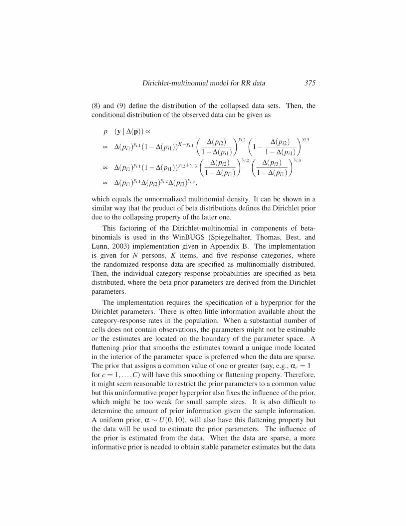
(8) and (9) define the distribution of the collapsed data sets. Then, the
conditional distribution of the observed data can be given as
p (y | Δ(p)) ∝
∝ Δ(pi1)yi.1(1−Δ(pi1))
K−yi.1
(Δ(pi2)
1−Δ(pi1)
)yi.2(
1− Δ(pi2)
1−Δ(pi1)
)yi.3
∝ Δ(pi1)yi.1(1−Δ(pi1))
yi.2+yi.3
(Δ(pi2)
1−Δ(pi1)
)yi.2(
Δ(pi3)
1−Δ(pi1)
)yi.3
∝ Δ(pi1)yi.1Δ(pi2)
yi.2Δ(pi3)yi.3 ,
which equals the unnormalized multinomial density. It can be shown in a
similar way that the product of beta distributions defines the Dirichlet prior
due to the collapsing property of the latter one.
This factoring of the Dirichlet-multinomial in components of beta-
binomials is used in the WinBUGS (Spiegelhalter, Thomas, Best, and
Lunn, 2003) implementation given in Appendix B. The implementation
is given for N persons, K items, and five response categories, where
the randomized response data are specified as multinomially distributed.
Then, the individual category-response probabilities are specified as beta
distributed, where the beta prior parameters are derived from the Dirichlet
parameters.
The implementation requires the specification of a hyperprior for the
Dirichlet parameters. There is often little information available about the
category-response rates in the population. When a substantial number of
cells does not contain observations, the parameters might not be estimable
or the estimates are located on the boundary of the parameter space. A
flattening prior that smooths the estimates toward a unique mode located
in the interior of the parameter space is preferred when the data are sparse.
The prior that assigns a common value of one or greater (say, e.g., αc = 1
for c = 1, . . . ,C) will have this smoothing or flattening property. Therefore,
it might seem reasonable to restrict the prior parameters to a common value
but this uninformative proper hyperprior also fixes the influence of the prior,
which might be too weak for small sample sizes. It is also difficult to
determine the amount of prior information given the sample information.
A uniform prior, α ∼ U(0,10), will also have this flattening property but
the data will be used to estimate the prior parameters. The influence of
the prior is estimated from the data. When the data are sparse, a more
informative prior is needed to obtain stable parameter estimates but the data
376 M. Avetisyan & J.-P. Fox
will be used to estimate the amount of prior information. Furthermore,
the estimated prior parameter estimates will reveal whether the observed
data do not support the model. In that case, a substantial amount of prior
information is needed, more than 20% of the sample data, to obtain stable
parameter estimates.
RESTRICTED DIRICHLET-MULTINOMIALMODELING
The Dirichlet-multinomial model in Equation (4) is a saturated model
in the sense that the category-response rates are freely estimated over
individuals. The Dirichlet prior does not impose any restrictions that are
typically present in a cross-classified data structure.
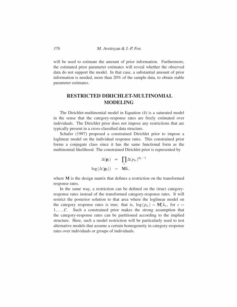
Schafer (1997) proposed a constrained Dirichlet prior to impose a
loglinear model on the individual response rates. This constrained prior
forms a conjugate class since it has the same functional form as the
multinomial likelihood. The constrained Dirichlet prior is represented by
Δ(pi) ∝ ∏c
Δ(pic)αc−1
log(Δ(pi)) = Mλ,
where M is the design matrix that defines a restriction on the transformed
response rates.
In the same way, a restriction can be defined on the (true) category-
response rates instead of the transformed category-response rates. It will
restrict the posterior solution to that area where the loglinear model on
the category response rates is true; that is, log(pic) = Mtcλc, for c =
1, . . . ,C. Such a constrained prior makes the strong assumption that
the category-response rates can be partitioned according to the implied
structure. Here, such a model restriction will be particularly used to test
alternative models that assume a certain homogeneity in category-response
rates over individuals or groups of individuals.
Dirichlet-multinomial model for RR data 377
APPLICATION OF THE DIRICHLET-MULTINOMIALMODEL
A simulation study is performed to evaluate the performance of the full
Bayes method for estimating the population proportions. Furthermore, the
full and empirical Bayes estimates of the true individual response rates are
compared under different conditions given categorical randomized response
data. Then, the model is used to analyze randomized response data from the
college alcohol problem scale (CAPS, O’Hare, 1997).
SIMULATION STUDY
In order to investigate the performance of the full Bayes estimation method,
data were simulated under various conditions. The number of persons (Nequaled 100 or 500), items (K equaled ten or fifteen), response categories (Cequaled three or five), and randomizing device characteristics (φ1 equaled .6
or .8) were varied. The data generation procedure comprised the following.
For each respondent C category-response rates were simulated from a
Dirichlet distribution given prior parameters α. The prior parameters were
constant or varied over response categories. For the constant case, the sum
of the prior parameters equaled C and the prior parameters equaled one such
that the population proportions equaled 1/C. For the non-constant case, the
sum of the prior parameters was not equal to C and the prior parameters
(α1,α2,α3) equaled (1,2,1) for C = 3 and (α1,α2,α3,α4,α5) equaled
(1,2,4,2,1) for C = 5. The simulated category-response rates were used
to generate true response patterns, which were randomized using the forced
response design with randomizing device probabilities φ1 and φ2 = 1/C.
Ten independent samples were generated for each condition.
The parameters were re-estimated using WinBUGS. The WinBUGS
code of the Dirichlet-multinomial model for RR data is given in Appendix
B. For each data set, 15,000 iterations were made with a burn-in period of
5,000 iterations. Each model parameter was estimated by the average of the
corresponding sampled values, which is an estimate of the posterior mean.
The method was successful in model parameter estimation. In both
cases, the point estimates are close to the true values and the standard
deviations become smaller when increasing the number of respondents.
Similar trends were found for the cases of three and five response categories.
However, for the C = 5 case, the reduction in the estimated prior weights
is better visible when increasing the number of items and/or decreasing
378 M. Avetisyan & J.-P. Fox
the percentage of forced responses. This follows from the fact that more
parameters need to be estimated with the same amount of observed data.
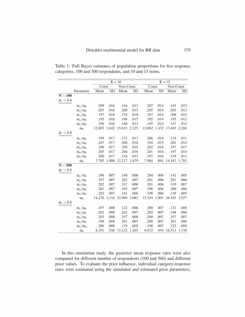
In Table 1, for C = 5, the estimated population proportions per category
are presented. The prior parameters were divided by the sum of the prior
parameters such that they were scaled in the same way as the true generating
values. Note that each estimate is an average of the estimates corresponding
to the ten independently generated data sets. It can be seen that the prior
parameter estimates resemble the true values quite well for the constant and
non-constant case. Increasing the number of persons leads to more accurate
results, since the estimated standard deviations become smaller.
When decreasing the percentage of forced responses, the standard
deviations remain constant for the case of ten and fifteen items, and 100
and 500 persons. The actual amount of information will increase when the
amount of forced responses is reduced, since the forced responses are just
random noise to mask the individual answers. From Equation (5) it can be
seen that the the number of items K as well as α0 determine the prior weight
in the computation of the individual expected posterior category-response
rate. It is clear that particularly for these situations the prior weights
reduce since the sum of the prior parameters become smaller. That is, the
influence of the population prior on the posterior mean category-response
rates becomes smaller when decreasing the amount of forced responses.
The observed RR data will contain more information about the individual
category-response rates when less forced responses are observed and less
prior information will be used to estimate the response rates. Note that the
standard deviations of the sum of the prior parameters (α0) become smaller
when decreasing the number of forced responses. The typical advantage of
the full Bayes estimation method applies here, where the prior weights are
also estimated from the data. Note that for φ1 = .6, 40% of the data are
forced responses. So, the actual amount of information in the data is rather
limited but the population parameters can still be recovered. The decrease
in the amount of forced responses leads to more accurate results.
When increasing the number of items, the standard deviations only
become slightly smaller. The additional amount of five RR observations
did not led to a substantial increase in the precision of the posterior mean
estimates. The increase in items led in to a higher estimate of α0 with a
smaller standard deviation. As a result, the posterior mean response rates
will be more influenced by the data than the prior information due to the
higher number of items and the higher posterior mean estimate of α0.
Dirichlet-multinomial model for RR data 379
Table 1: Full Bayes estimates of population proportions for five response
categories, 100 and 500 respondents, and 10 and 15 items.
K = 10 K = 15
Const. Non-Const. Const. Non-Const.
Parameter Mean SD Mean SD Mean SD Mean SD
N = 100φ1 = 0.6
α1/α0 .209 .016 .144 .013 .207 .014 .145 .012
α2/α0 .203 .016 .200 .015 .205 .014 .205 .013
α3/α0 .197 .016 .318 .018 .197 .014 .308 .015
α4/α0 .195 .016 .198 .015 .195 .014 .195 .013
α5/α0 .196 .016 .140 .013 .195 .014 .147 .012
α0 12.003 1.642 15.615 2.225 12.082 1.432 17.445 2.204
φ1 = 0.8
α1/α0 .199 .017 .123 .013 .206 .016 .114 .011
α2/α0 .207 .017 .208 .016 .194 .015 .201 .014
α3/α0 .190 .017 .350 .019 .202 .016 .357 .017
α4/α0 .205 .017 .204 .016 .201 .016 .197 .014
α5/α0 .200 .017 .116 .012 .197 .016 .119 .011
α0 7.785 1.008 12.217 1.679 7.984 .861 14.183 1.781
N = 500φ1 = 0.6
α1/α0 .196 .007 .140 .006 .204 .006 .141 .005
α2/α0 .197 .007 .203 .007 .201 .006 .201 .006
α3/α0 .202 .007 .321 .008 .201 .006 .319 .007
α4/α0 .201 .007 .195 .007 .196 .006 .200 .006
α5/α0 .203 .007 .141 .006 .198 .006 .139 .005
α0 14.276 1.116 22.994 2.083 15.534 1.001 26.183 2.057
φ1 = 0.8
α1/α0 .197 .008 .122 .006 .200 .007 .122 .005
α2/α0 .202 .008 .201 .007 .202 .007 .198 .006
α3/α0 .203 .008 .357 .008 .200 .007 .357 .007
α4/α0 .198 .008 .201 .007 .200 .007 .201 .006
α5/α0 .200 .008 .119 .005 .198 .007 .122 .005
α0 8.351 .526 15.232 1.265 8.672 .454 16.511 1.110
In this simulation study, the posterior mean response rates were also
compared for different number of respondents (100 and 500) and different
prior values. To evaluate the prior influence, individual category-response
rates were estimated using the simulated and estimated prior parameters,
380 M. Avetisyan & J.-P. Fox
and through a full Bayes estimation method. Per response category, the
mean squared error (MSE) of the estimated response rates was calculated.
The MSE comprises a comparison of the estimate of the individual response
rate with the true value. For category c, the MSE can be stated as
MSE(pc | y) =N
∑i=1|c
E(pic − pic)2 +
N
∑i=1|c
Var(pic)2,
where the first term is the cumulative bias between the true value and its
estimate and the second term represents the cumulative variance of the
estimate.
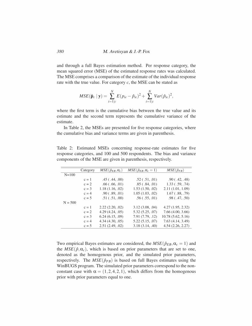
In Table 2, the MSEs are presented for five response categories, where
the cumulative bias and variance terms are given in parenthesis.
Table 2: Estimated MSEs concerning response-rate estimates for five
response categories, and 100 and 500 respondents. The bias and variance
components of the MSE are given in parenthesis, respectively.
Category MSE(pEB,αc) MSE(pEB,αc = 1) MSE(pFB)N=100
c = 1 .45 ( .44, .00) .52 ( .51, .01) .90 ( .42, .48)
c = 2 .66 ( .66, .01) .85 ( .84, .01) 1.33 ( .59, .74)
c = 3 1.18 (1.16, .02) 1.53 (1.50, .02) 2.11 (1.01, 1.09)
c = 4 .90 ( .89, .01) 1.05 (1.03, .02) 1.67 ( .88, .79)
c = 5 .51 ( .51, .00) .56 ( .55, .01) .98 ( .47, .50)
N = 500
c = 1 2.22 (2.20, .02) 3.12 (3.08, .04) 4.27 (1.95, 2.32)
c = 2 4.29 (4.24, .05) 5.32 (5.25, .07) 7.66 (4.00, 3.66)
c = 3 6.24 (6.15, .09) 7.91 (7.79, .12) 10.78 (5.62, 5.16)
c = 4 4.34 (4.30, .05) 5.22 (5.15, .07) 7.63 (4.14, 3.49)
c = 5 2.51 (2.49, .02) 3.18 (3.14, .40) 4.54 (2.26, 2.27)
Two empirical Bayes estimates are considered, the MSE( pEB,αc = 1) and
the MSE( p,αc), which is based on prior parameters that are set to one,
denoted as the homogenous prior, and the simulated prior parameters,
respectively. The MSE(pFB) is based on full Bayes estimates using the
WinBUGS program. The simulated prior parameters correspond to the non-
constant case with α = (1,2,4,2,1), which differs from the homogenous
prior with prior parameters equal to one.
Dirichlet-multinomial model for RR data 381
For 100 and 500 persons, the bias is smallest for the full Bayes
estimates and they are slightly better than empirical Bayes estimates given
the true prior parameters. The full Bayes estimates are accurate with
respect to bias since the prior weights are also estimated from the sampled
data. The estimates using the homogenous prior, with all prior parameters
equal to one, have the highest bias but smaller MSEs than those based
on the full Bayes estimates. For the latter one, the estimated variances
are much higher due to the fact that the prior parameters also need to
be estimated. Therefore, the homogenous prior leads to quite accurately
estimated category-response rates and performs better than the full Bayes
estimates given the MSEs.
RESPONSE RATES OF ALCOHOL-RELATED NEGATIVECONSEQUENCES
The college alcohol problem scale (CAPS; OHare, 1997) was used
to measure frequencies of alcohol-related negative consequences among
college students. Thirteen items of the CAPS scale were used that
covered socio-emotional problems (hangovers, memory loss, nervousness,
depression) and community problems (drove under the influence, engaged
in activities related to illegal drugs, problems with the law). Each item has
a five-point scale (one = never/almost never, five =almost always).
A total of 793 US college student were at random divided in two groups.
One group of 351 participants answered the questionnaire directly without
using a randomizing device, denoted as the direct-questioning (DQ) group.
The other group, denoted as the RR group, consisted of 442 participants
and they responded to the questionnaire according to a forced randomized
response design, where φ1 = .60 and φ2(c) = .20 for c = 1, . . . ,5. The RR
group used a spinner to answer the questions. The spinner was developed
such that 60% of the area was comprised of answer honestly space, and 40%
of the area was divided into equal sections to represent the five possible
answer choices.
The main focus of the study was to investigate whether the RR technique
improved the accuracy of self-reports. The sensitivity of the response
categories was evaluated, where it was expected that a strong confirmation
to an item is more sensitive than a negative confirmation. The Dirichlet-
multinomial model with a restricted Dirichlet prior was used to evaluate
the effect of the RR technique per category, where the between-group
382 M. Avetisyan & J.-P. Fox
differences in mean category-response rates were investigated.
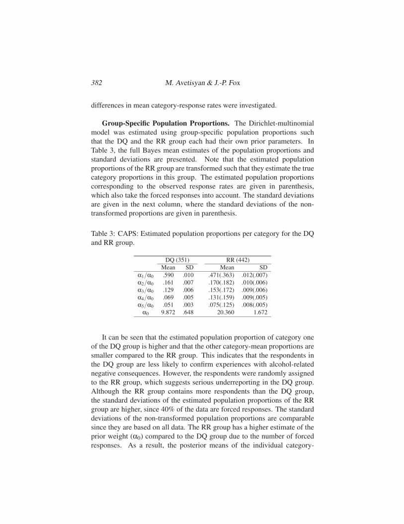
Group-Specific Population Proportions. The Dirichlet-multinomial
model was estimated using group-specific population proportions such
that the DQ and the RR group each had their own prior parameters. In
Table 3, the full Bayes mean estimates of the population proportions and
standard deviations are presented. Note that the estimated population
proportions of the RR group are transformed such that they estimate the true
category proportions in this group. The estimated population proportions
corresponding to the observed response rates are given in parenthesis,
which also take the forced responses into account. The standard deviations
are given in the next column, where the standard deviations of the non-
transformed proportions are given in parenthesis.
Table 3: CAPS: Estimated population proportions per category for the DQ
and RR group.
DQ (351) RR (442)
Mean SD Mean SD
α1/α0 .590 .010 .471(.363) .012(.007)
α2/α0 .161 .007 .170(.182) .010(.006)
α3/α0 .129 .006 .153(.172) .009(.006)
α4/α0 .069 .005 .131(.159) .009(.005)
α5/α0 .051 .003 .075(.125) .008(.005)
α0 9.872 .648 20.360 1.672
It can be seen that the estimated population proportion of category one
of the DQ group is higher and that the other category-mean proportions are
smaller compared to the RR group. This indicates that the respondents in
the DQ group are less likely to confirm experiences with alcohol-related
negative consequences. However, the respondents were randomly assigned
to the RR group, which suggests serious underreporting in the DQ group.
Although the RR group contains more respondents than the DQ group,
the standard deviations of the estimated population proportions of the RR
group are higher, since 40% of the data are forced responses. The standard
deviations of the non-transformed population proportions are comparable
since they are based on all data. The RR group has a higher estimate of the
prior weight (α0) compared to the DQ group due to the number of forced
responses. As a result, the posterior means of the individual category-
Dirichlet-multinomial model for RR data 383
response rates are more influenced by the prior in the RR group than in
the DQ group.
Linear Restricted Category Response Rates. To investigate the category-
specific effect of the RR method, a loglinear model was defined for the
category-response rates. For each category, the logarithm of the true
category-response rates were explained by a constant and a category-
specific RR effect. This restriction of the Dirichlet prior is given by
log(pic) = λ0c +λ1cRRi,
for c = 1, . . . ,C, where RRi equals one when respondent i belongs to the RR
group and zero otherwise. Note that the loglinear representation was only
used to evaluate the category-specific RR effect.
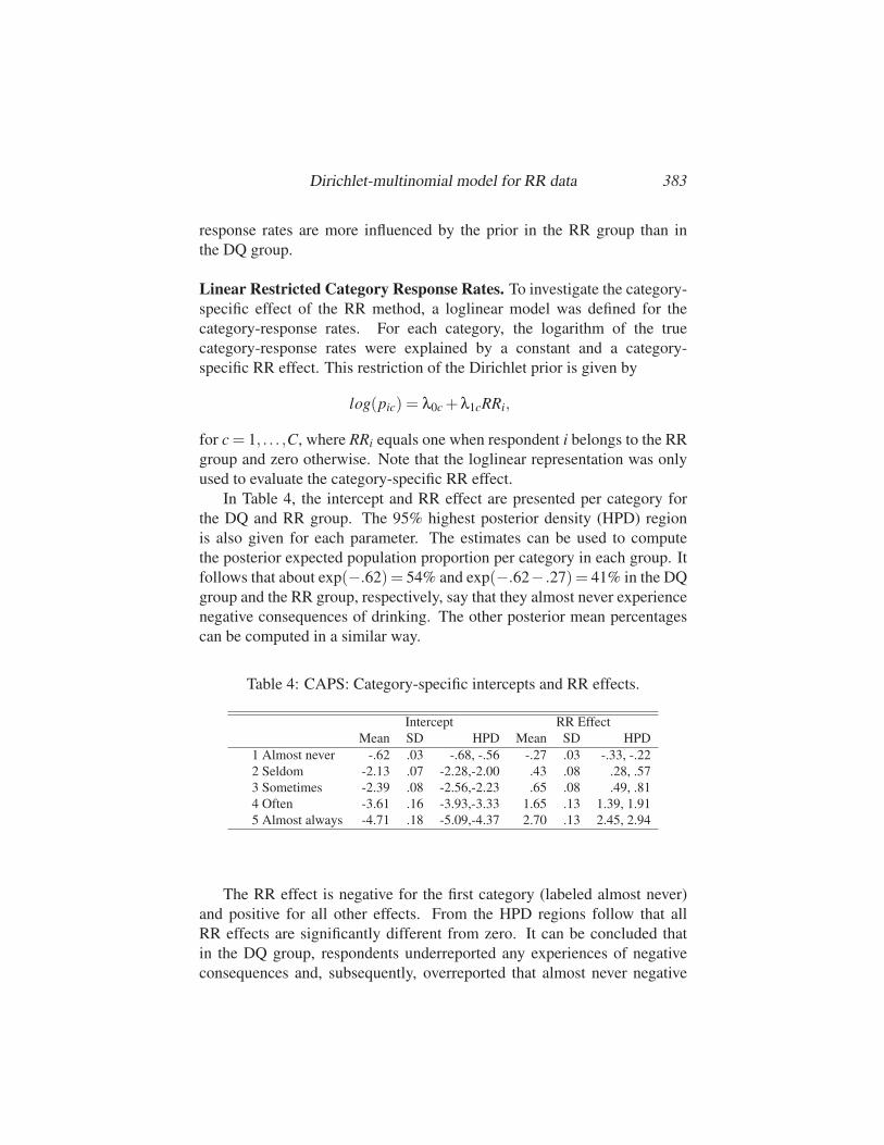
In Table 4, the intercept and RR effect are presented per category for
the DQ and RR group. The 95% highest posterior density (HPD) region
is also given for each parameter. The estimates can be used to compute
the posterior expected population proportion per category in each group. It
follows that about exp(−.62) = 54% and exp(−.62− .27) = 41% in the DQ
group and the RR group, respectively, say that they almost never experience
negative consequences of drinking. The other posterior mean percentages
can be computed in a similar way.
Table 4: CAPS: Category-specific intercepts and RR effects.
Intercept RR Effect
Mean SD HPD Mean SD HPD
1 Almost never -.62 .03 -.68, -.56 -.27 .03 -.33, -.22
2 Seldom -2.13 .07 -2.28,-2.00 .43 .08 .28, .57
3 Sometimes -2.39 .08 -2.56,-2.23 .65 .08 .49, .81
4 Often -3.61 .16 -3.93,-3.33 1.65 .13 1.39, 1.91
5 Almost always -4.71 .18 -5.09,-4.37 2.70 .13 2.45, 2.94
The RR effect is negative for the first category (labeled almost never)
and positive for all other effects. From the HPD regions follow that all
RR effects are significantly different from zero. It can be concluded that
in the DQ group, respondents underreported any experiences of negative
consequences and, subsequently, overreported that almost never negative
384 M. Avetisyan & J.-P. Fox
consequences were experienced. Furthermore, the estimated RR effects
increase with an increase in the number of negative experiences, where the
fifth category has the highest RR effect. Thus, an increase in the number
of experiences of alcohol-related negative consequences leads to a more
sensitive response option. The difference between the groups with respect
to the posterior expected proportion of respondents that admits experiencing
negative consequences is highest for the fifth response option. In that case,
around 1% of the DQ group admits to have almost always alcohol-related
negative consequences, which is around 13% in the RR group. It can be
concluded that the RR technique led to a higher degree of cooperation and
more accurate data, especially when the response options become more
sensitive.
The response data from the RR group were used to explore ethnic
differences in experiencing alcohol-related negative consequences. The
responses from the DQ group were shown to be biased, since effects of
under- and overreporting were found. In this study, the racial origin of the
respondents was administered. The RR group consisted of 2% Asians, 83%
white Americans, 11% African Americans, and 12% belonged to another
race. An indicator variable, labeled Ethnicity, was used in the log-linear
model that represented the racial origin of each respondent.
In Table 5, the estimated category-specific effects of ethnicity on the
individual category response rates are given. Each posterior mean effect is
accompanied with a posterior standard deviation (SD) and a 95% highest
posterior density (HPD) interval. Under the column labeled Effect, the
estimated effects are represented, where each category-specific intercept
represents the average population level on the logarithmic scale. Under
the column labeled Scaled Effect, the intercept represents the average
population level of the African Americans on the logarithmic scale. The
scaled ethnic effect of the this group is in that case equal to zero.
For the first category, the African Americans score significantly higher
than the other groups. Furthermore, the estimated scaled effects of the
other groups are significantly smaller. This means that the percentage
of African-Americans experiencing almost never negative consequences is
much higher compared to the other groups. In the same way, it follows that
the percentage of African-Americans experiencing negative consequences
seldom to almost always is lower than that of other groups. In the second
category, the white Americans also score significantly higher than the
African Americans, which follows from the scaled effects. The third to
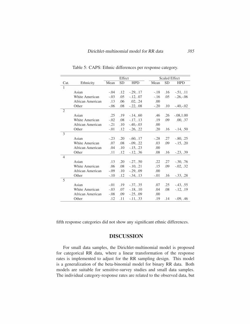
Dirichlet-multinomial model for RR data 385
Table 5: CAPS: Ethnic differences per response category.
Effect Scaled Effect
Cat. Ethnicity Mean SD HPD Mean SD HPD
1
Asian -.04 .12 -.29, .17 -.18 .16 -.51, .11
White American -.03 .05 -.12, .07 -.16 .05 -.26,-.06
African American .13 .06 .02, .24 .00
Other -.06 .08 -.22, .08 -.20 .10 -.40,-.02
2
Asian .25 .19 -.14, .60 .46 .26 -.08,1.00
White American -.02 .08 -.17, .13 .19 .09 .00, .37
African American -.21 .10 -.40,-.03 .00
Other -.01 .12 -.26, .22 .20 .16 -.14, .50
3
Asian -.23 .20 -.60, .17 -.28 .27 -.80, .25
White American .07 .08 -.09, .22 .03 .09 -.15, .20
African American .04 .10 -.15, .23 .00
Other .11 .12 -.12, .36 .08 .16 -.23, .39
4
Asian .13 .20 -.27, .50 .22 .27 -.30, .76
White American .06 .08 -.10, .21 .15 .09 -.02, .32
African American -.09 .10 -.29, .09 .00
Other -.10 .12 -.34, .13 -.01 .16 -.33, .28
5
Asian -.01 .19 -.37, .35 .07 .25 -.43, .55
White American -.03 .07 -.18, .10 .04 .08 -.12, .19
African American -.08 .09 -.25, .09 .00
Other .12 .11 -.11, .33 .19 .14 -.09, .46
fifth response categories did not show any significant ethnic differences.
DISCUSSION
For small data samples, the Dirichlet-multinomial model is proposed
for categorical RR data, where a linear transformation of the response
rates is implemented to adjust for the RR sampling design. This model
is a generalization of the beta-binomial model for binary RR data. Both
models are suitable for sensitive-survey studies and small data samples.
The individual category-response rates are related to the observed data, but
386 M. Avetisyan & J.-P. Fox
a linear transformation can be used to derive the true categorical-response
rates. The parameters of this linear transformation are the characteristics
of the randomizing device and they are usually known. The derived
expressions of the posterior expectation and variance of the category-
response rates are useful in case of empirical Bayes estimation or explicit
prior knowledge about response rate population parameters.
The idea of full Bayes parameter estimation was elaborated using the
synthetic data set. The simulation study has shown that full Bayes model
was able to rather accurately estimate values of parameters for different
number of response categories. The method was equally successful
in retrieving the parameters for the constant case of homogenous prior
parameters as well as for the case of non-constant prior parameters.
Moreover, the simulation study concluded that increasing the number of
persons leads to more accurate results, while the variation of the percentage
of forced responses does not influence the accuracy.
A constrained-Dirichlet prior is used to identify homogeneity in
response rates over items and persons. Therefore, the WinBUGS program
was extended to define a constrained-Dirichlet prior, where a loglinear
model was defined on the true category-response rates.
An important effect was identified in the real data study, which showed
that the effect of the RR method varied over response categories. A priori
it was assumed that the response options varied in their sensitivity, where a
higher degree of accordance with the sensitive item but this hypothesis was
never tested in the literature. The analysis showed a substantial increase
in agreement with more sensitive response options under the randomized
response condition.
In RR studies the topic of compliance is often an issue. Respondents
are instructed to follow the RR instructions but may for different reasons
act differently. In large-scale sample studies, a latent class structure can be
integrated in the model to identify non-compliant behavior. The responses
from the non-compliant subjects are modeled differently. The Dirichlet-
multinomial model can also be extended with a two-component latent-class
structure to allow for non-compliance, but that would require more response
data to obtain stable parameter estimates.
Dirichlet-multinomial model for RR data 387
REFERENCES
Brier, S. S. (1980). Analysis of contingency tables under cluster sampling.
Biometrika, 67, 591−596.
Bockenholt, U., & van der Heijden, P. G. M. (2007). Item-
randomized response models for measuring noncompliance: Risk-
return perception, social influences, and self-protective responses.
Psychometrika, 72, 245−262.
Danaher, P. J. (1988). Parameter estimation for the Dirichlet-
multinomial distribution using supplementary beta-binomial data.
Communications in Statistics - Theory and Methods, 17, 1777−1788.
Dishon, M., & Weiss, G. H. (1980). Small sample comparison of
estimation methods for the Beta distribution. Journal of StatisticalComputation and Simulation, 11, 1−11.
De Jong, M. G., Pieters, R., & Fox, J.-P. (2010). Reducing social
desirability bias through item randomized response: An application
to measure underreported desires. Journal of Marketing Research,47, 14−27.
Edgell, S. E., Himmelfarb, S., & Duchan, K. L. (1982). The validity
of forced responses in a randomized response model. SociologicalMethods and Research, 11, 89−100.
Fox, J.-P. (2005). Randomized item response theory models. Journal ofEducational and Behavioral Statistics, 30, 189−212.
Fox, J.-P. (2008). Beta-binomial ANOVA for multivariate randomized
response data. British Journal of Mathematical and StatisticalPsychology, 61, 453−470.
Fox, J.-P., & Wyrick, C. (2008). A mixed effects randomized item
response model. Journal of Educational and Behavioral Statistics,33, 389−415.
Greenberg, B. G., Abul-Ela, A.-L. A., Simmons, W. R., & Horwitz,
D. G. (1969). The unrelated question randomized response
model: Theoretical framework. Journal of the American StatisticalAssociation, 64, 520−539.
388 M. Avetisyan & J.-P. Fox
Goodhardt, G. J., Ehrenberg, A. S. C., & Chatfield, C. (1984). The
Dirichlet: A comprehensive model of buying behavior. Journal ofthe Royal Statistical Society. Series A (General), 147, 621−655.
Mosimann, J. E. (1962). On the compound multinomial distribution,
the multivariate β-distribution, and correlations among proportions.
Biometrika, 49, 65−82.
O’Hare, T. M. (1997). Measuring problem drinkers in first time offenders:
Development and validation of the Collage Alcohol Problem Scale
(CAPS). Journal of Substance Abuse Treatment, 14, 383−387.
Paul, S. R., Balasooriya, U., & Banerjee, T. (2005). Fisher information
matrix of the Dirichlet-multinomial distribution.
Biometrical Journal, 47, 230−236.
Schafer, J. L. (1997). Analysis of incomplete multivariate data. London:
Chapman & Hall.
Spiegelhalter, D. J., Thomas, A., Best, N., & Lunn, D. (2003).
WinBUGS User Manual, Version 1.4 Retrieved from http://www.mrc-
bsu.cam.ac.uk /bugs/winbugs/manual14.pdf.
Tourangeau, R., Rips, L. J., & Rasinski, K. (2000). The psychology ofsurvey response. Cambridge, England: Cambridge University Press.
Tourangeau, R., & Yan, T. (2007). Sensitive questions in surveys.
Psychological Bulletin, 133, 859−883.
Warner, S. L. (1965). Randomized response: A survey technique for
eliminating evasive answer bias. Journal of the American StatisticalAssociation, 60, 63−69.
Wilson, J. R., & Chen, G. S. C. (2007). Dirichlet-multinomial model
with varying response rates over time. Journal of Data Science, 5,
413−423.
Dirichlet-multinomial model for RR data 389
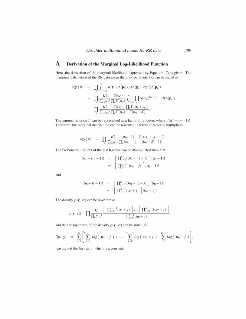
A Derivation of the Marginal Log-Likelihood Function
Here, the derivation of the marginal likelihood expressed by Equation (7) is given. The
marginal distribution of the RR data given the prior parameters α can be stated as
p(y | α) = ∏i
∫Δ(pi)
p(yi. | Δ(pi)) p(Δ(pi) | α)d(Δ(pi))
= ∏i
K!
∏c yi.c!
Γ(α0)
∏c Γ(αc)
∫Δ(pi)
∏c
Δ(pic)αc+yi.c−1d(Δ(pi))
= ∏i
K!
∏c yi.c!
Γ(α0)
∏c Γ(αc)
∏c Γ(αc + yi.c)
Γ(α0 +K).
The gamma function Γ can be represented as a factorial function, where Γ(n) = (n− 1)!.Therefore, the marginal distribution can be rewritten in terms of factorial multipliers.
p(y | α) = ∏i
K!
∏c yi.c!
(α0 −1)!
∏c(αc −1)!
∏c(αc + yi.c −1)!
(α0 +K −1)!.
The factorial multipliers of the last fraction can be manipulated such that
(αc + yi.c −1)! =[
∏yi.cj=1((αc −1)+ j)
](αc −1)!
=[
∏yi.c−1j=0 (αc + j)
](αc −1)!
and
(α0 +K −1)! =[
∏Kj=1((α0 −1)+ j)
](α0 −1)!
=[
∏K−1j=0 (α0 + j)
](α0 −1)!.
The density p(y | α) can be rewritten as
p(y | α) = ∏i
K!
∏c yi.c!
[∏yi.1−1
j=0 (α1 + j)]. . .
[∏yi.C−1
j=0 (αC + j)]
∏K−1j=0 (α0 + j)
and the the logarithm of the density p(y | α) can be stated as
l(α | y) ∝N
∑i=1
[yi.1−1
∑j=0
log(
α1 + j)+ . . .+
yi.C−1
∑j=0
log(
αC + j)−K−1
∑j=0
log(
α0 + j)]
,
leaving out the first term, which is a constant.

390 M. Avetisyan & J.-P. Fox
B WinBUGS Code of the Multinomial-Dirichlet Model
The code of the Dirichlet-multinomial model for RR data is given for N persons, K items,
and five response categories. The randomizing device has parameters φ1 and φ2.
model
{f o r ( i i n 1 :N)
{y [ i , 1 : 5 ] ˜ d m u l t i ( q [ i , ] , K)
q [ i , 1 ] ˜ d b e t a ( a l p h a [ 1 ] , b e t a t o t 1 )
q 2 s t a r [ i ] ˜ d b e t a ( a l p h a [ 2 ] , b e t a t o t 2 )
q [ i ,2]<− q 2 s t a r [ i ]∗(1−q [ i , 1 ] )
q 3 s t a r [ i ] ˜ d b e t a ( a l p h a [ 3 ] , b e t a t o t 3 )
q [ i ,3]<− q 3 s t a r [ i ]∗(1−q [ i ,1]−q [ i , 2 ] )
q 4 s t a r [ i ] ˜ d b e t a ( a l p h a [ 4 ] , a l p h a [ 5 ] )
q [ i ,4]<− q 4 s t a r [ i ]∗(1−q [ i ,1]−q [ i ,2]−q [ i , 3 ] )
q [ i ,5]<−1−q [ i ,1]−q [ i ,2]−q [ i ,3]−q [ i , 4 ]
}
a l p h a [ 1 ] ˜ d u n i f ( 0 , 1 0 )
a l p h a [ 2 ] ˜ d u n i f ( 0 , 1 0 )
a l p h a [ 3 ] ˜ d u n i f ( 0 , 1 0 )
a l p h a [ 4 ] ˜ d u n i f ( 0 , 1 0 )
a l p h a [ 5 ] ˜ d u n i f ( 0 . 5 , 1 0 )
a lpha0<−sum ( a l p h a [ 1 : 5 ] )
b e t a t o t 1 <−sum ( a l p h a [ 2 : 5 ] )
b e t a t o t 2 <−sum ( a l p h a [ 3 : 5 ] )
b e t a t o t 3 <−sum ( a l p h a [ 4 : 5 ] )
f o r ( i i n 1 :N)
{ f o r ( c i n 1 : 5 )
{p [ i , c ] <− ( q [ i , c ] − (1− ph i1 )∗ ph i2 ) / ph i1
}}
}
Recommended