THE EFFECTS OF REFRACTIVE INDEX MISMATCH ON
MULTIPHOTON FLUORESCENCE EXCITATION
MICROSCOPY OF BIOLOGICAL TISSUE
Pamela Anne Young
Submitted to the faculty of the University Graduate School in partial fulfillment of the requirements
for the degree Doctor of Philosophy
in the Program of Biomolecular Imaging and Biophysics Indiana University
July 2010

ii
Accepted by the Faculty of Indiana University, in partial fulfillment of the requirements for the degree of Doctor of Philosophy.
_____________________________________
Kenneth W. Dunn, Ph.D., Chair
_____________________________________
Robert L. Bacallao, M.D.
Doctoral Committee
_____________________________________
Ricardo S. Decca, Ph.D.
June 17, 2010
_____________________________________
Michael Rubart, M.D.

iii
ACKNOWLEDGEMENTS
I would like to thank my mentor, Dr. Ken Dunn, for teaching me how to be a
scientist.
I would also like to thank the other members of my research committee: Dr.
Robert Bacallao, Dr. Ricardo Decca, and Dr. Michael Rubart. Dr. Decca, thank you for
the hours at the whiteboard in your office, answering the millions of emails I sent you,
and your incredible patience. Dr. Bacallao, thank you for excellent advice, the off the
wall questions that were always exactly relevant enough to stretch my mind but never
anything I would have thought of on my own, and your fantastic jokes. Dr. Rubart, thank
you for your endless support, your thoughts and advice, and your incredibly prompt
replies to my emails. I would not have been able to complete this dissertation project
without you.
I would like to thank Dr. Simon Atkinson, my program director, for encouraging
me to join the new graduate program in Biomolecular Imaging. I would like to thank Dr.
Bruce Molitoris, the director of the Indiana Center for Biological Microscopy and
chairman of the Nephrology Division of the Department of Medicine, for his support and
encouragement.
Additionally, I would like to thank Jason Byars for his hours of programming in
an attempt to minimize my masochism. I would like to thank Sherry Clendenon, my
partner in crime. I would like to thank Cliff Babbey for always listening and lending
advice. I would like to thank George Rhodes for training me in animal surgery and
intravital microscopy. I would like to thank Ruben Sandoval for training me and helping

iv
me over and over again. I would like to thank Jeff Clendenon for being an endless
resource of information about microscopy and image processing. I would like to thank
Bruce Henry for helping me with the microscopy. I would like to thank Exing Wang for
designing the excitation path on the microscope where I conducted the majority of my
experiments and for training me in alignment of the system. I would like to thank
Heather Ward for teaching me how to fix and store tissue samples and trying to teach me
Amira.
I would also like to thank all of my friends for supporting me through graduate
school, especially Sarah Wean, Nicci Knipe, Henry Mang, David Southern, Stacy
Bennett, Keri Jeter, Nikki Ray, and Tabitha Hardy.
Finally, I would like to thank my family for their endless support.
This work was supported by a George M. O’Brien award from the NIH (P30 DK
079312-01) and conducted at the Indiana Center for Biological Microscopy.

v
ABSTRACT
Pamela Anne Young
THE EFFECTS OF REFRACTIVE INDEX MISMATCH ON MULTIPHOTON
FLUORESCENCE EXCITATION MICROSCOPY OF BIOLOGICAL TISSUE
Introduction: Multiphoton fluorescence excitation microscopy (MPM) is an
invaluable tool for studying processes in tissue in live animals by enabling biologists to
view tissues up to hundreds of microns in depth. Unfortunately, imaging depth in MPM
is limited to less than a millimeter in tissue due to spherical aberration, light scattering,
and light absorption. Spherical aberration is caused by refractive index mismatch
between the objective immersion medium and sample. Refractive index heterogeneities
within the sample cause light scattering. We investigate the effects of refractive index
mismatch on imaging depth in MPM.
Methods: The effects of spherical aberration on signal attenuation and resolution
degradation with depth are characterized with minimal light absorption and scattering
using sub-resolution microspheres mounted in test sample of agarose with varied
refractive index. The effects of light scattering on signal attenuation and resolution
degradation with depth are characterized using sub-resolution microspheres in kidney
tissue samples mounted in optical clearing media to alter the refractive index
heterogeneities within the tissue.
Results: The studies demonstrate that signal levels and axial resolution both
rapidly decline with depth into refractive index mismatched samples. Interestingly,

vi
studies of optical clearing with a water immersion objective show that reducing scattering
increases reach even when it increases refractive index mismatch degrading axial
resolution. Scattering, in the absence of spherical aberration, does not degrade axial
resolution. The largest improvements in imaging depth are obtained when both scattering
and refractive index mismatch are reduced.
Conclusions: Spherical aberration, caused by refractive index mismatch between
the immersion media and sample, and scattering, caused by refractive index
heterogeneity within the sample, both cause signal to rapidly attenuate with depth in
MPM. Scattering, however, seems to be the predominant cause of signal attenuation with
depth in kidney tissue.
Kenneth W. Dunn, Ph.D., Chair
vii
TABLE OF CONTENTS
I. Introduction ....................................................................................................................1
A. Multiphoton fluorescence excitation microscopy in biomedical research ...............1
B. Multiphoton fluorescence excitation microscopy ....................................................3
1. Multiphoton fluorescence excitation ...................................................................3
2. Lasers ...................................................................................................................7
3. Beam intensity control .........................................................................................8
4. Beam expander collimator ...................................................................................9
5. Beam scanner .....................................................................................................10
6. Objectives ..........................................................................................................10
7. Detectors ............................................................................................................12
C. Single-photon versus two-photon microscopy.......................................................14
D. Imaging depth limitations of MPM........................................................................18
1. Spherical aberration ...........................................................................................18
a. Point spread function .................................................................................20
b. Axial scaling ..............................................................................................22
c. Signal attenuation.......................................................................................23
d. Resolution ..................................................................................................24
2. Scattering ...........................................................................................................24
3. Absorption .........................................................................................................26
E. Optical clearing ......................................................................................................27
F. Hypothesis..............................................................................................................29
viii
II. Materials and Methods .................................................................................................31
A. Sample preparation ................................................................................................31
1. Agarose sample preparation...............................................................................31
2. Microsphere labeling .........................................................................................31
3. Immunofluorescence ..........................................................................................32
4. Mounting media .................................................................................................33
B. Two-photon microscopy ........................................................................................33
C. Signal attenuation and resolution degradation .......................................................36
1. Excitation and Emission Spectra .......................................................................36
2. Fluorescence Saturation .....................................................................................37
3. Image collection .................................................................................................38
4. Signal attenuation analysis.................................................................................38
5. Resolution degradation analysis ........................................................................40
D. Excitation attenuation ............................................................................................41
1. Image collection .................................................................................................41
2. Excitation attenuation analysis ..........................................................................42
3. Excitation attenuation calibration data collection ..............................................44
E. Emission attenuation ..............................................................................................45
1. Calculation based on signal and excitation data ................................................45
2. Comparison of descanned and non-descanned detectors ...................................46
F. Analysis of outliers ................................................................................................46
G. Immunofluorescence image collection ..................................................................47

ix
III. Results ..........................................................................................................................48
Chapter 1. The Effect of Spherical Aberration on Multiphoton Microscopy ............48
A. Alignment of the two-photon excitation light path ................................................48
B. Characterization of suncoast yellow 0.2 micron microspheres .............................48
C. Effects from the media at the coverslip .................................................................52
D. Fluorescence saturation ..........................................................................................52
E. Signal attenuation...................................................................................................57
F. Resolution degradation ..........................................................................................59
G. Excitation attenuation ............................................................................................61
1. Photobleaching rate............................................................................................61
2. Excitation power versus photobleaching rate ....................................................63
H. Emission attenuation ..............................................................................................63
1. Fluorescence signal versus fluorescence excitation...........................................63
2. Comparison of descanned and non-descanned detectors ...................................66
I. Signal attenuation in kidney tissue ........................................................................66
1. Comparison of agarose and kidney tissue samples ............................................66
2. Comparison of water and oil immersion objectives ..........................................69
Chapter 2. The effect of refractive index heterogeneity in multiphoton
microscopy of kidney tissue.................................................................................71
A. The effect of mounting media refractive index on signal attenuation with
depth in kidney tissue using a water immersion objective ....................................71
B. The effect of mounting media refractive index on resolution degradation
with depth in kidney tissue using a water immersion objective ............................73

x
C. The effect of reducing both refractive index heterogeneity and mismatch
on signal attenuation with depth in kidney tissue ..................................................75
D. The effect of reducing both refractive index heterogeneity and mismatch
on resolution degradation .......................................................................................81
Chapter 3. Mathematical model of refractive index mismatch in MPM using
geometric optics ....................................................................................................83
A. Theory ....................................................................................................................83
B. MATLAB ...............................................................................................................92
1. Overview ............................................................................................................92
2. Intensity program ...............................................................................................94
3. Optimize D program ..........................................................................................96
4. Optimize D Range program ...............................................................................98
5. Overnight OD program ......................................................................................98
6. Model calculations .............................................................................................99
C. Comparison to empirical data ................................................................................99
IV. Discussion ..................................................................................................................104
A. Summary ..............................................................................................................104
B. The effect of refractive index mismatch on signal attenuation ............................105
C. The effect of refractive index mismatch on excitation attenuation ......................106
D. The effect of refractive index mismatch on emission attenuation .......................107
E. Signal attenuation in kidney tissue ......................................................................107
F. Axial resolution degradation in kidney tissue ......................................................109
G. Geometrical model of refractive index mismatch in MPM .................................111

xi
V. Conclusions ................................................................................................................114
VI. Future Studies ............................................................................................................115
VII. Appendices ...............................................................................................................117
A. Geometrical model ...............................................................................................117
1. Overnight OD program ....................................................................................117
2. Optimize D Range program .............................................................................117
3. Optimize D program ........................................................................................117
4. Intensity program .............................................................................................119
B. ImageJ plugins .....................................................................................................122
1. Getting_Loaded_Olympus.java .......................................................................122
2. Pam_Background.java .....................................................................................127
3. Pam_Bead_Stats.java .......................................................................................129
4. Pam_Bead_Stats2.java .....................................................................................137
5. Pam_Bead_Stats3.java .....................................................................................150
6. Pam_Bead_StatsMedian.java ..........................................................................165
7. Pam_Bead_StatsResolution.java .....................................................................196
C. Excel macros ........................................................................................................219
1. Common_Tools ...............................................................................................219
2. Pam_Tools .......................................................................................................227
3. Resolution_Tools .............................................................................................257
VIII.References ................................................................................................................284
Curriculum Vitae

xii
LIST OF TABLES
Table 1. Comparison of confocal and multiphoton microscopy .......................................17
Table 2. Mounting media ..................................................................................................34
Table 3. Objective lens parameters ...................................................................................84
Table 4. Global variables ..................................................................................................97

xiii
LIST OF FIGURES
Figure 1. Jablonski diagram ...............................................................................................4
Figure 2. Fluorescence excitation for one-and two-photon microscopy............................6
Figure 3. Schematic of Keplerian beam expander/collimator .........................................11
Figure 4. Refractive index mismatch broadens the focal point .......................................19
Figure 5. Effect of correction collar adjustments on the point spread functions
of fluorescent microspheres .............................................................................21
Figure 6. Beam expander/collimator ................................................................................35
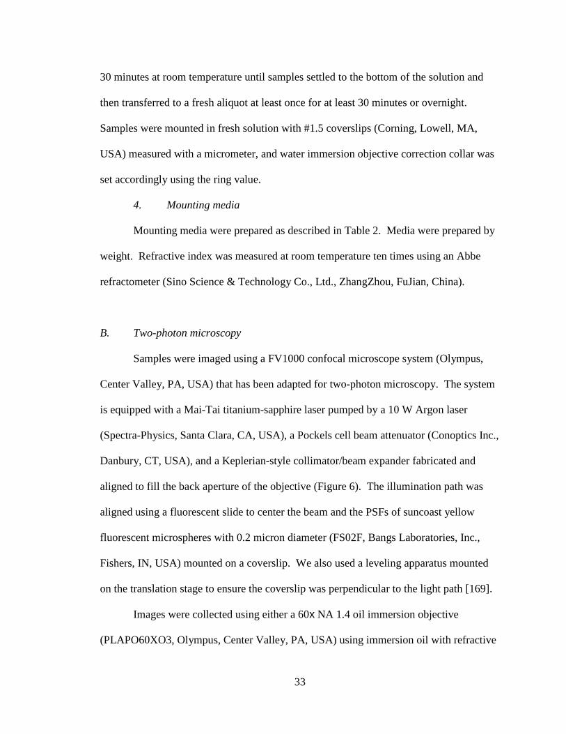
Figure 7. Beam expander/collimator alignment ...............................................................49
Figure 8. Excitation spectra for suncoast yellow 0.2 micron microspheres ....................50
Figure 9. Emission spectra for suncoast yellow 0.2 micron microspheres ......................51
Figure 10. Comparison of fluorescence intensity at the coverslip-sample interface
for samples with different refractive index ......................................................53
Figure 11. Fluorescence Saturation Data ..........................................................................54
Figure 12. Fluorescence Saturation Data ..........................................................................55
Figure 13. Fluorescence Saturation Data ..........................................................................56
Figure 14. Fluorescence signal attenuation .......................................................................58
Figure 15. Axial resolution degradation ...........................................................................60
Figure 16. Photobleaching rate attenuation ......................................................................62
Figure 17. Calibration data ...............................................................................................64
Figure 18. Emission attenuation .......................................................................................65
Figure 19. Comparison of descanned and non-descanned detector ..................................67

xiv
Figure 20. Signal attenuation in kidney tissue ..................................................................68
Figure 21. Water immersion objective versus oil immersion objective ...........................70
Figure 22. Qualitative study of signal attenuation caused by refractive index
heterogeneity using water immersion objective .............................................72
Figure 23. Quantitative study of signal attenuation caused by refractive index
heterogeneity using water immersion objective .............................................74
Figure 24. Quantitative study of resolution degradation caused by refractive index
heterogeneity using water immersion objective .............................................76
Figure 25. Qualitative study of signal attenuation caused by refractive index
heterogeneity using oil immersion objective ..................................................77
Figure 26. Quantitative study of signal attenuation caused by refractive index
heterogeneity using oil immersion objective ..................................................79
Figure 27. Optimization of refractive index heterogeneity and mismatch .......................80
Figure 28. Quantitative study of resolution degradation caused by refractive index
heterogeneity using oil immersion objective ..................................................82
Figure 29. Model schematic ..............................................................................................85
Figure 30. Model schematic ..............................................................................................87
Figure 31. Model schematic ..............................................................................................89
Figure 32. Model schematic ..............................................................................................91
Figure 33. Model schematic ..............................................................................................93
Figure 34. Model calculations.........................................................................................100
Figure 35. Model calculations.........................................................................................101
Figure 36. Comparison of model and empirical data ......................................................102

xv
LIST OF ABBREVIATIONS
AFP
AOM
BABB
CCD
CLSM
EOM
DMSO
FWHM
GaAs
GaAsP
GFP
MPM
NA
Nd:YVO4
NFP
PBS
PEG
PMT
PSF
RFP
Ti:S
Actual focal position
Acousto-optic modulator
Benzyl alcohol/benzyl benzoate
Cooled charge-coupled device
Confocal fluorescence laser scanning microscopy
Electro-optic modulator
Dimethyl sulfoxide
Full width at half maximum
Gallium arsenide
Gallium arsenide phosphide
Green fluorescent protein
Multiphoton fluorescence excitation microscopy
Numerical aperture
Neodymium doped yttrium orthvanadate
Nominal focal position
Phosphate buffered saline
Polyethylene glycol
Photomultiplier tube
Point spread function
Red fluorescent protein
Titanium sapphire

1
I. INTRODUCTION
A. Multiphoton fluorescence excitation microscopy in biomedical research
In vivo imaging techniques have become widely utilized in biology. Techniques,
such as positron emission tomography (PET), single photon emission computed
tomography (SPECT), and magnetic resonance imaging (MRI), are excellent for studying
whole organs and tissues but have spatial and temporal resolution that are too poor to
characterize cellular processes at sub-second timescales [1]. Multiphoton fluorescence
excitation microscopy (MPM) enables biologists to study processes hundreds of microns
in depth in tissue in live animals with submicron resolution and timescales of seconds or
less [2-13]. As a fluorescence technique, MPM can be used to localize multiple specific
molecules simultaneously. MPM has also been shown to have low photon toxicity,
allowing extended observation of highly sensitive processes without detectable damage
[14]. MPM offers biologists the capability of characterizing cellular and subcellular
processes deep into tissues in three dimensions in the context of tissues and organs in
living animals.
In brain tissue, the first tissue to be studied using MPM, images were collected of
neurons in invertebrate ganglia, mammalian brain slices, and intact mammalian brains
[15, 16]. Since then MPM has been used to study blood flow [17-20], dendritic spine
behavior [21-27], calcium dynamics in dendrites [28-33] and presynaptic boutons [34-
36], and microglia cell dynamics [37, 38]. The effects of plaques on dendritic structure
and dendritic spines have been examined in Alzheimer studies [39-42]. MPM has also
been used for in vivo studies of stroke in mice [43, 44].

2
There have been numerous studies of the immune system to examine lymphocyte
dynamics in vivo [45-56] and study model antigen systems to examine immune responses
to infection in vivo [57-62]. Immune system studies using MPM have examined skin
[63-65], spinal cord [66], gut [67], bone marrow [68, 69], and liver [70]. MPM has also
been used to study intracellular signaling [71, 72], cell proliferation [55], chemotaxis [73-
80], and T cell effector function [65, 81, 82].
MPM has also enabled biologists to study the cardiovascular system to examine
calcium transients and study cellular transplantation in Langendorff-perfused mouse
hearts [83-85]. Research has also been done using MPM to examine lymphocyte
infiltration into atherosclerotic arteries [86].
In live rats and mice, the kidney has been externalized and apposed to a coverslip
on the stage of the microscope, and MPM images have been directly collected for
measurement of basic renal physiological parameters [3, 87], including glomerular
filtration and permeability, tubular fluid and blood flow, urinary concentration/dilution,
and rennin content and release [88-92]. This method has also been used for studies of
acute renal failure [93-95], microvascular leakage in a rat model of renal ischemia [96,
97], folic acid uptake and transport [98], organic anion transport [7], bacterial infections
[57, 59-62], and nephrotoxicity of aminoglycoside antibiotics [99, 100]. Fixed
embryonic kidneys from a mouse model of polycystic kidney disease have been studied
to characterize renal development [101, 102].

3
B. Multiphoton fluorescence excitation microscopy
1. Multiphoton fluorescence excitation
Conventional fluorescence microscopy generates images by exciting fluorescent
molecules, whether endogenous to the sample or added exogenously, allowing
investigators to collect images of the distribution and behavior of these specific
molecules. Short wavelengths of light excite the fluorescent molecule from the ground
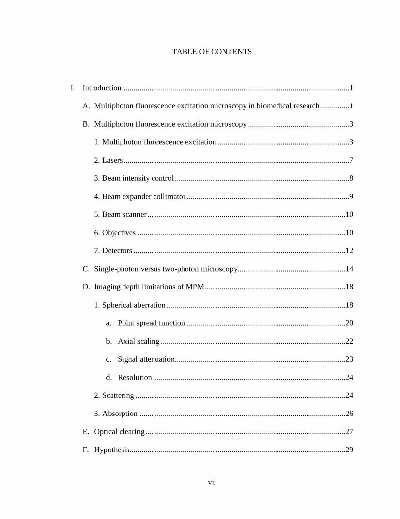
electronic state to an excited electronic state (Figure 1). Within each electronic state are
vibrational states. The fluorescence molecule then loses a small amount of energy as heat
as the molecule relaxes to a lower vibrational state. It then relaxes back to the ground
state, emitting a photon with less energy and a longer wavelength than the excitation
light. The difference between the excitation and emission wavelengths is known as the
Stokes shift. A dichromatic mirror is used to separate the excitation wavelengths from
the emission wavelengths, generating images with extremely high contrast. By
specifically labeling multiple molecules in a tissue with spectrally distinct fluorophores,
researchers can collect images of distributions of multiple molecules in the same sample
to compare spatial relationships. Samples are excited sequentially with wavelengths
specific for each probe, and fluorescence emissions are collected using barrier filters
optimized for collection of each separate probe.
Unlike single-photon fluorescence excitation, multiphoton fluorescence excitation
is based on a nonlinear process where two or more low energy photons are absorbed by a
fluorescent molecule exciting the molecule to fluoresce (Figure 1). In the case of two-
photon fluorescence excitation, this requires that the summed energy of the two photons
be equal to the energy required to stimulate an electronic transition to a higher energy

4
Figure 1. Jablonski diagram Jablonski diagram demonstrating one- and two-photon fluorescence excitation. Two-photon excitation results from the simultaneous absorption of two low-energy photons by a fluorophore.
5
state. Because energy is inversely proportional to wavelength, the wavelength of the two
photon excitation spectra is generally approximately twice that of the single photon
excitation spectra, typically optimal between 700-1000 nm. In order for two photons to
stimulate an electronic transition, they must arrive within the lifetime of the virtual
excitation state, approximately 10-16 seconds [5, 11, 103]. The probability that two-
photon excitation will occur depends quadratically on the excitation power and is very
low when typical energies are used for single-photon fluorescence microscopy [104].
The probability is improved to generate sufficient signal by pulsing near-infrared laser
light temporally and focusing the light spatially with an objective lens [5] (Figure 2).
Rapidly but briefly pulsing the laser generates a peak power sufficient to excite two-
photon fluorescence but an average power low enough to avoid harming the sample. A
typical MPM system generates a peak photon flux approximately one million times that
at the surface of the sun [12]. However, it has been show to be gentle enough not to harm
developing hamster embryos [14].
Focusing the illuminating light spatially with an objective lens will create a
conical geometry of the illuminating beam, causing the photon density to decrease with
the square of axial distance from the focal plane. This, combined with the quadratic
dependence of two-photon excitation, results in fluorescence decreasing with the fourth
power of axial distance from the focus. Therefore, the photon density is only sufficient to
cause two-photon excitation at the focus in a volume dependent upon the excitation
wavelength, refractive index, and numerical aperture (NA) of the objective. High NA
objectives make it possible to collect subfemtoliter focal volumes [11]. Because

6
Figure 2. Fluorescence excitation for one- and two-photon microscopy In one-photon fluorescence microscopy, a continuous wave ultraviolet or visible light laser excites fluorophores throughout the volume. In two-photon microscopy, an infrared laser provides pulsed illumination such that the density of photons sufficient for simultaneous absorption of two photons by fluorophores only occurs at the focal point.

7
fluorescence excitation is localized to a single point in the sample, an image is formed by
scanning the focus across the sample. A photomultiplier tube collects the emitted
fluorescence to build up the image point by point. In order to acquire images in
reasonable periods of time, each point in the sample is imaged very briefly, on the order
of microseconds.
2. Lasers
MPM was first introduced in 1990 by Denk et al., who were able to generate the
extremely high photon flux required for two-photon fluorescence excitation with
appreciable probability [103]. They achieved this by combining the tight focusing of a
laser scanning microscope with the temporal concentration from a 25 mW colliding-
pulse, mode-locked dye laser (Clark Instruments, Pittsford, NY) (λ~630 nm) to produce a
stream of pulses with 100 fs pulse duration at about 80 MHz repetition rate.
Unfortunately, femtosecond dye lasers, like those they used, are impractical for the
average biologist. Not only are they toxic, requiring regular dye changes leading to
generation of a lot of toxic waste, but they also are difficult to tune, with changes of
greater than 30 nm requiring an entire dye change [105].
However, in 1992, a “home-built” self-sustaining mode-locked titanium sapphire
(Ti:S) crystal-based laser was applied to MPM [106]. Ti:S lasers have become the most
common MPM excitation sources available. They consist of a pair of two separate lasers,
a continuous-wave diode pump laser (typically Neodymium Doped Yttrium Orthvanadate
(Nd:YVO4) crystal-based laser) and Ti:S laser, or may be in a single box containing both
the pump laser and the Ti:S oscillator. Ti:S lasers use broadband optics so that the
wavelength can be tuned within the range of 690-1020 nm, two-laser, or 720-920 nm,

8
single-box [11]. Many of these lasers are now computer-controlled, making them
extremely user-friendly. The laser power available varies depending on the pump laser
but ranges from 5-10 W pump, providing an average power of up to 1-2 W at the Ti:S
peak wavelengths. However, a mode-locked Ti:S laser produces a pulsed laser beam
with extremely high peak power.
A laser is “mode-locked” when only a certain set of frequencies are propagating
in the laser cavity, with the phase between these frequencies creating destructive
interference between all of the propagating frequencies except at one point in the cavity
where the waves add constructively, resulting in a single short pulse of light. Typical
mode-locked lasers have a pulse duration with full width at half maximum (FWHM) of
80-150 fs [11]. The distance between the two cavity end mirrors determines the
repetition rate, typically ~80 MHz. Because femtosecond Ti:S lasers require many
intracavity frequencies, the pulses have a large spectral bandwidth, typically with FWHM
of ~10 nm, with a symmetrical Gaussian shape. The pulse duration and spectral
bandwidth are related, therefore if the pulse passes through a dispersive media, because
longer wavelengths travel faster than shorter wavelengths, the pulse becomes “positively
chirped,” increasing the pulse duration but not changing the spectrum. Pulse broadening
reduces the photon flux, decreasing two-photon fluorescence excitation. Lasers are
available for MPM that correct for group velocity dispersion by adding negative
dispersion to pre-chirp the laser.
3. Beam intensity control
The laser intensity can be controlled by neutral-density filters, a rotatable
polarizer, an electro-optic modulator (EOM), or an acousto-optic modulator (AOM).

9
Neutral-density filters attenuate laser intensity independent of wavelength and come in
two general types, absorptive gray glass filters or reflective metallic filters [107].
Because MPM utilizes high laser powers, absorptive gray glass filters may overheat.
Graded neutral density filters and filter wheels are good for general attenuation but are
not fast enough to blank the beam during retrace with a linear galvanometer scanner.
Fast shuttering requires an EOM or AOM. An EOM uses a crystal, such as
lithium niobate or gallium arsenide, that produces birefringence, induced by an electric
field, to control laser intensity. Laser beam attenuation is controlled by varying the
voltage applied to the Pockels cell. An EOM can also be used to modulate the phase, the
frequency, or the direction of propagation of the laser beam [107]. EOMs have very high
throughput, but incomplete extinction [108]. An AOM modulates the laser intensity
using the optical effects of an acoustic field on a birefringent crystal [107]. A
piezoelectric crystal is attached to the birefringent crystal and generates an acoustic field.
The frequency of the acoustic wave affects the local density of crystal, and therefore the
refractive index, creating a periodic diffractor. Light passing through the crystal is
diffracted at an angle depending on the wavelength of light and frequency of the acoustic
wave. The intensity of the deflected beam can be varied from 0-85% and switched on an
off with a high extinction ratio. The dispersive materials used in EOMs and AOMs
spread the laser pulse temporally, decreasing photon flux, and therefore the optical
system would benefit from prechirping [108].
4. Beam expander collimator
A beam expander can be used to adjust the beam width of the laser at the back
aperture of the objective. Underfilling the back aperture of the objective elongates and

10
enlarges the illumination profile at the focus of the objective and reduces the effective
numerical aperture. Filling and overfilling the back aperture result in a diffraction-
limited focus.
There are two main types of beam expanders. The Galilean type consists of a
negative lens causing the beam to diverge followed by a positive lens that collimates the
beam. The Keplerian type consists of two positive lenses with wither focal points
coincident (Figure 3). The Keplerian type beam expander can also be used in
conjunction with a spatial filter to remove the scattered components of the beam. The
spatial filter consists of a pinhole positioned at the focus of the converging beam.
5. Beam scanner
MPM typically uses mirrors mounted on galvanometer motors to scan the focused
laser beam across the sample. XY scanner designs include nonresonant linear
galvanometers or resonant galvanometers [11]. Nonresonant linear galvanometers raster
scan the beam, using a sawtooth pattern with a relatively slow linear recording time
followed by a fast retrace [107]. The benefit of linear galvanometers is that they have
adjustable scan speed, providing a digital zoom and the ability to rotate the scan axis
[11]. Resonant galvanometers use a torsion spring to vibrate at a fixed frequency so
recording time is during the trace and retrace [107]. They are able to achieve much faster
scan rates but are not as capable of zooming, panning, or rotating [11].
6. Objectives
For two-photon excitation to occur with appreciable probability, the laser must be
condensed temporally, by pulsing, and spatially, using an objective lens to form a tight

11
Figure 3. Schematic of Keplerian beam expander/collimator The schematic depicts D0 is the beam width of the incident light, f0 is the focal length of the first lens, f1 is the focal length of the second lens and d1 is the beam width of the expanded beam.

12
focus [5]. Because the objective lens in MPM acts as the condenser and objective, it
needs to have excellent optics to form a tight focus and to provide good throughput to
minimize light loss. Therefore ideal objective lenses use optics that have been optimized
to transmit visible and near-infrared wavelengths. Although MPM can be achieved using
low or high NA objectives, MPM benefits from the use of high NA objective not only
because of the tight focus but also because of the large collection angle, enabling high
NA objectives to collect more scattered emissions [109].
High NA objectives are available with water, glycerol, or oil immersion. Because
oil has the highest refractive index, these objectives are capable of having the highest
NA. However when focusing deep into an aqueous sample, refractive index mismatch
causes spherical aberration which degrades image quality. Therefore water and glycerol
immersion objectives are frequently the better choice for biological imaging. Water and
glycerol objectives have been designed with a correction collar on the objective lens that
moves optical elements inside the lens to correct for refractive index mismatch caused by
coverslip thickness variation. This correction collar can also be used to correct for
temperature-dependent index changes and the refractive index of the sample [110, 111].
A useful comparison of many objective lenses available from Leica Microsystems
(Wetzlar, Germany), Carl Zeiss MicroImaging (GmbH, Germany), Nikon Instruments
Inc. (Tokyo, Japan), and Olympus (Tokyo, Japan) can be found in reference [112].
7. Detectors
In MPM, three-dimensional localization is accomplished by excitation alone,
making numerous detection options available. The most commonly used type of non-
descanned detection is whole-area detection where fluorescence light passes through the
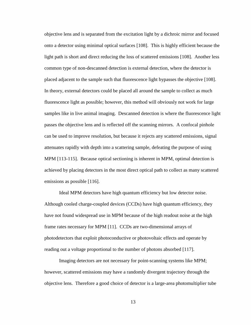
13
objective lens and is separated from the excitation light by a dichroic mirror and focused
onto a detector using minimal optical surfaces [108]. This is highly efficient because the
light path is short and direct reducing the loss of scattered emissions [108]. Another less
common type of non-descanned detection is external detection, where the detector is
placed adjacent to the sample such that fluorescence light bypasses the objective [108].
In theory, external detectors could be placed all around the sample to collect as much
fluorescence light as possible; however, this method will obviously not work for large
samples like in live animal imaging. Descanned detection is where the fluorescence light
passes the objective lens and is reflected off the scanning mirrors. A confocal pinhole
can be used to improve resolution, but because it rejects any scattered emissions, signal
attenuates rapidly with depth into a scattering sample, defeating the purpose of using
MPM [113-115]. Because optical sectioning is inherent in MPM, optimal detection is
achieved by placing detectors in the most direct optical path to collect as many scattered
emissions as possible [116].
Ideal MPM detectors have high quantum efficiency but low detector noise.
Although cooled charge-coupled devices (CCDs) have high quantum efficiency, they
have not found widespread use in MPM because of the high readout noise at the high
frame rates necessary for MPM [11]. CCDs are two-dimensional arrays of
photodetectors that exploit photoconductive or photovoltaic effects and operate by
reading out a voltage proportional to the number of photons absorbed [117].
Imaging detectors are not necessary for point-scanning systems like MPM;
however, scattered emissions may have a randomly divergent trajectory through the
objective lens. Therefore a good choice of detector is a large-area photomultiplier tube

14
(PMT) [118, 119]. PMTs use a photocathode that absorbs signal photons, producing
photoelectrons which are amplified by charge multiplication, producing a signal current
[120]. The current is then digitized in intervals based on the timing of the scanning
mirrors such that each pixel value in the image represents the signal intensity during the
brief time period the appropriate area of the sample is being imaged [121]. PMTs have a
rapid response and high gain, for a good dynamic range, but low quantum efficiency [11].
This is because most photons are either transmitted or reflected rather than absorbed and
therefore do not contribute to the signal [120]. However, gallium arsenide (GaAs) and
gallium arsenide phosphide (GaAsP) PMTs have markedly higher quantum efficiency
than traditional multi-alkali PMTs [11, 120].
C. Single-photon versus two-photon microscopy
Conventional fluorescence microscopy generates images with extremely high
contrast by exciting fluorescent molecules in a sample, then collecting the fluorescence
emissions while rejecting the excitation light. This works well for thin samples;
however, thick samples generate fluorescence throughout the sample, causing out-of-
focus fluorescence to appear in the image. Out-of-focus fluorescence reduces contrast
[122] and the signal-to-noise ratio [123]. This problem was first addressed in 1957 with
the development of the confocal fluorescence microscope [124]. Confocal fluorescence
microscopy uses a set of conjugate apertures located in the illumination and detection
path to ensure that the microscope illuminates and detects from the same focal volume.
These pinholes function as spatial filters to eliminate stray light, rejecting out-of-focus
fluorescence, effectively collecting an “optical section” within the thick sample.

15
Confocal fluorescence microscopy has advanced since 1957. Today, confocal
fluorescence laser scanning microscopy (CLSM) is a technique that uses laser light to
excite fluorescence in the sample and galvanometer scanning mirrors to raster scan the
focus across the sample to build an image. By repeating this for multiple focal planes an
image volume of the sample can be collected.
MPM and CLSM are very similar techniques. Both types of microscopy use point
scanning to collect optical sections of the sample. Surprisingly, MPM and CLSM have
similar resolution. Because CLSM uses ultraviolet and visible excitation wavelengths
and MPM uses near-infrared, about twice the wavelength, the Rayleigh criterion predicts
that under ideal conditions CLSM will have lateral resolution of approximately
𝑟𝑥𝑦,𝑐𝑜𝑛𝑓𝑜𝑐𝑎𝑙 ≈0.4𝜆𝑒𝑚𝑁𝐴
and MPM will have lateral resolution of approximately
𝑟𝑥𝑦,𝑚𝑝𝑚 ≈0.7𝜆𝑒𝑚𝑁𝐴
where 𝜆𝑒𝑚 is the emission wavelength and 𝑁𝐴 is the numerical aperture of the objective
[125]. Similarly, axial resolution is predicted to be
𝑟𝑧,𝑐𝑜𝑛𝑓𝑜𝑐𝑎𝑙 ≈1.4𝜆𝑒𝑚𝑛𝑁𝐴2
𝑟𝑧,𝑚𝑝𝑚 ≈2.3𝜆𝑒𝑚𝑛𝑁𝐴2
where 𝑛 is the refractive index of the objective lens immersion fluid [125]. However,
“ideal imaging conditions” are rarely achieved. Frequently, when collecting images with
CLSM, samples are dim causing a low signal-to-noise ratio which reduces resolution
[125]. By opening up the pinhole, more signal can be collected, improving signal-to-

16
noise ratio, but this is also at the expense of resolution [125]. Typical pinhole
adjustments result in CLSM resolution similar to MPM [11].
Though both CLSM and MPM can be used to collect image volumes, MPM is
inherently better for deep tissue imaging. MPM utilizes near-infrared wavelengths of
light (700-1000 nm) for excitation. These wavelengths are within an “optical window” in
the absorption spectrum of biological tissue, making them ideal for imaging biological
samples [6]. Also, because Rayleigh scattering has a wavelength dependence of ~λ-4,
these longer excitation wavelengths scatter less than shorter wavelengths, improving
imaging depth compared to CLSM [116].
MPM also has that advantage that no pinhole is required to collect an optical
section. This means that all of the fluorescent emissions come from the focus and can be
collected to form the image. Therefore, large-area detectors can be placed in the light
path close to the objective lens, eliminating light loss from optical elements in the
descanning path and scattering. Calculations have shown that nearly all of the
fluorescence stimulated 100 microns deep in tissue are scattered before exiting the tissue
[5, 119]. Centonze and White [116] have shown that using descanned detectors, MPM
improves imaging depth 2-fold over CLSM. They have also shown that using non-
descanned detectors, imaging depth improves three-fold over that of MPM with
descanned detectors.
Another important advantage of MPM over CLSM is that photobleaching and
photodamage are minimized [126]. CLSM excites fluorescence throughout the entire

Table 1. Comparison of confocal and multiphoton microscopy
17

18
double-inverted cone of light leading to photobleaching and photodamage anywhere that
cone intersects the sample [126]. MPM uses near-infrared excitation light and only
excites the sample at the focus, a much smaller area exposed to photobleaching and
photodamage [11]. However, it is important to note that MPM can still lead to
considerable photodamage and photobleaching in the focal volume. In fact,
photobleaching, expected to occur in proportion to the square of excitation power, has
actually been shown to occur at higher-order [127].
D. Imaging depth limitations of MPM
Although MPM improves fluorescence signal with depth over other fluorescence
techniques, imaging depth is still limited. Fluorescence signals can be expected to
attenuate with depth in tissues due to reduced stimulation of fluorescence or reduced
detection of fluorescence. This is caused by spherical aberration, light scattering, and
absorption of light [5, 11, 110, 111, 115, 116, 119, 128-132]. Both excitation and
detection of fluorescence at depth are sensitive to scattering and absorption of light.
Spherical aberration is caused by refractive index mismatch between the objective
immersion fluid and sample and will also limit signal at depth.
1. Spherical aberration
Although MPM has many advantages over CLSM with respect to imaging deep
into biological tissue, MPM is still depth-limited. Deep tissue imaging typically involves
imaging into a medium whose refractive index does not match that of the objective
immersion fluid. Refractive index mismatch between the immersion fluid, coverslip, and

19
Figure 4. Refractive index mismatch broadens the focal point Schematic (not to scale) of excitation light path. Dashed line indicates ideal case where sample refractive index is 1.515, matching immersion oil. Red line indicates excitation light path into sample with refractive index less than 1.515. The ideal case comes to a sharp focus, but when the sample has a different refractive index than the objective immersion fluid, the light bends upon encountering the sample, broadening the focal point.

20
sample causes spherical aberration [110, 111, 115, 128, 131, 132]. Spherical aberration
is a condition where the focal point is broadened due to the peripheral rays of light
coming to focus at a different place than the paraxial rays (Figure 4). Spherical
aberration is an on-axis aberration. However, since MPM uses galvanometer scanning
mirrors to raster scan the focal point of light to build the image, refractive index
mismatch in MPM causes minor off-axis aberrations as well.
a. Point spread function
The effect of spherical aberration can be visualized by collecting images of the
point spread function (PSF). The PSF describes the three-dimensional light intensity
distribution at the focus and is a convolution of the illumination PSF, the light intensity
distribution for the illumination process, and detection PSF, the probability that a
fluorescent photon is able to propagate to the detector. The PSF can be visualized by
collecting images of sub-resolution fluorescent microspheres. Figure 5 shows XZ cross-
sectional images of 0.5 micron red fluorescent microspheres (F8812, Invitrogen, Eugene,
OR, USA). Imaging was conducted using the Olympus FV1000 confocal microscope
system that has been adapted for two-photon microscopy by the Indiana Center for
Biological Microscopy. A Mai Tai Ti:S laser (Spectra-Physics, Mountain View, CA,
USA) provided the excitation light at wavelength 800 nm. Image volumes were collected
using a water immersion objective (Olympus, 60x Plan Apochromat, NA 1.2) designed
for use with glass coverslips. Since correction for spherical aberration critically depends
upon coverslip thickness, such objectives are equipped with correction collars. This
collar moves the objective lens elements so that the paraxial and peripheral rays of light
form a tight focus after traveling through a glass coverslip of defined thickness.

21
Figure 5. Effect of correction collar adjustments on the point spread functions of fluorescent microspheres XZ cross-section of 0.5 micron fluorescent microspheres mounted immediately below the coverslip with collar settings (A) 0.13, (B) 0.17, and (C) 0.21 mm. Pseudocolor based on intensity. Scale bar = 2 microns. X=Z.

22
Conversely, the collar can be used to manipulate spherical aberration in a particular
sample. In Figure 5, the images were collected with the objective collar adjusted for a
nominal 0.13 mm thickness (A), 0.17 mm thickness (B), and 0.21 mm thickness (C).
Since the coverslip was measured to be 0.180 ± 0.001 mm thick, it is not surprising that
the best results were obtained using the nominal 0.17 mm collar setting, which generated
compact and vertically symmetrical PSFs (Figure 5B).
Adjusting the collar to 0.13 mm introduced negative spherical aberration into the
imaging system (Figure 5A). Negative spherical aberration results from the refractive
index of the sample being greater than the refractive index of the immersion fluid,
resulting in displacement of peripheral rays to a deeper focus than axial rays. This causes
diffraction rings that, when imaged using CLSM or MPM, extend toward the objective
lens. In Figure 5A, this is reflected by the asymmetrical formation of rings projecting
towards the objective lens.
Adjusting the collar to 0.21 mm resulted in positive spherical aberration (Figure
5C). Positive spherical aberration results from the refractive index of the sample being
less than the refractive index of the immersion fluid, as in the case of imaging with an oil
objective into water. Positive spherical aberration results in displacement of peripheral
rays to a shallower focus than axial rays causing diffraction rings that, when imaged
using CLSM or MPM, extend more intensely deeper into the sample. In Figure 5C, this
is reflected by the formation of rings projecting away from the objective lens.
b. Axial scaling
Spherical aberration also results in axial scaling [132]. Axial scaling refers to the
image volume being either compressed or stretched axially. Negative spherical

23
aberration results in an axially compressed image volume. Positive spherical aberration
results in an image volume that is stretched axially. This is caused by the peripheral rays
not focusing to the same place as the paraxial rays, resulting in a focal shift. The focal
shift is the difference between the actual focal position (AFP) and the nominal focal
position (NFP). The NFP is the distance between the coverslip and the focus in a system
with refractive indices that are perfectly matched. Imaging depth is typically measured
by the physical axial movement of the objective lens, which reflects the NFP. The AFP
can be approximated from the NFP using the paraxial approximation, the ratio of the
refractive index of the sample to the refractive index of the immersion medium [133].
The axial scaling factor is the ratio between the AFP and NFP. The axial scaling factor
has been measured using CLSM and used to determine the correct thickness and
refractive index of a sample [134, 135].
c. Signal attenuation
Since broadening of the image of the focal spot results in the rejection of
fluorescence by the confocal pinhole, spherical aberration significantly reduces the
collection of fluorescence at depth in confocal microscopy. The use of large area
detectors makes the effects of spherical aberration on fluorescence collection much less
pronounced in MPM [5]. Thus the fluorescence detection system of a multiphoton
microscope makes it much less susceptible to the effects of both scattering and spherical
aberration on signal collection.
However, the quality of the illumination focus, which is critically important to
efficient multiphoton fluorescence stimulation, may be an issue that can be addressed to
significantly improve MPM at depth. Because multiphoton fluorescence excitation is

24
critically dependent upon a tightly focused, diffraction limited spot, degradation of the
focal spot will lead to decreased photon density and quadratically decreased fluorescence.
It is well understood that spherical aberration degrades the tight focus of illumination
light, and accordingly, studies in model systems have shown MPM will be highly
sensitive to spherical aberration [115, 131, 136-138].
d. Resolution
Spherical aberration may also cause axial resolution degradation with depth. By
broadening the focus, spherical aberration reduces resolution in widefield microscopy
[139]. Because of the confocal pinhole, the effects of spherical aberration on resolution
are not nearly as significant in CLSM [140]. The effects of spherical aberration on
MPM are hard to predict. Focal broadening results in a decreased photon flux, but a high
photon flux is crucial for achieving appreciable two-photon excitation. Therefore,
resolution may decrease as the focus broadens, or it may not be affected because the
photon density is insufficient to excite two-photon fluorescence. While some studies
indicate that resolution of MPM decreases with depth into biological tissues [141, 142],
other studies find no such effect [116, 130, 143]. However studies that have specifically
looked at the effect of spherical aberration have found that resolution decreases with
depth [131, 136, 143].
2. Scattering
Scattering is a predominant factor ultimately limiting the reach of MPM.
Scattering results from refractive index heterogeneities in the tissue, for example from
cell membranes or intracellular structures [144]. Biological samples are heterogeneous
and do not have a uniform refractive index [145-147]. Kidney tissue, for example, is

25
made up of a rich vasculature, renal corpuscles, renal tubules, and covered in a fibrous
capsule. This is unfortunate for biologists interested in using microscopy to study the
kidney because the light path through kidney tissue has many interfaces where light is
refracted and reflected, and even light in the “optical window” is strongly scattered [145].
Scattering arises due to refractive index mismatch at the boundaries between these
inhomogeneities, such as at the extracellular fluid-cell membrane interface. Calculations
have shown that nearly all of the fluorescence stimulated 100 microns deep in tissue are
scattered before exiting the tissue [5, 119], making large-area detectors necessary for
deep tissue imaging.
Because MPM can efficiently collect scattered light, scattering primarily impacts
imaging depth by reducing power at the focus of illumination. Studies indicate that
scattered photons do not contribute to two-photon excitation [5, 131, 143, 148]. Imaging
depth ultimately is limited by the relative amount of excitation at the focus versus
shallower depths. The decrease in fluorescence excitation caused by light scattering and
absorption can be addressed by increasing laser power with depth into the sample or
using a regenerative amplifier, at least up to the fundamental depth limit.
Scattering has been shown to fundamentally limit imaging depth [129]. In brain
tissue, the fundamental imaging depth was found to be ~1 mm [9]. A regenerative
amplifier was used as the excitation source to lower repetition rates while maintaining the
average power, significantly increasing depth penetration. However, depth was limited
by an increase in out-of-focus fluorescence from the surface of the sample. Near-surface
fluorescence is caused by scattered excitation light, increasing the background signal
such that fluorescence excited at the focus cannot be discerned from the background

26
levels. This was first reported by Ying et al. [142]. They described that with increasing
scattering strength of the sample, the location of the maximum fluorescence intensity
moves away from the focal region toward the surface of the sample where it is more
evenly distributed, causing loss of the optical sectioning ability inherent in MPM.
By decreasing refractive index heterogeneity, the ultimate depth limit can be
addressed. Reducing refractive index heterogeneity reduces scattering and out-of-focus
fluorescence at the surface of the sample, thereby increasing the fundamental depth limit.
Using excitation powers below the level that causes out-of-focus fluorescence, it
is difficult to predict how scattering will affect resolution. It seems unlikely that
scattered light would contribute to the focus. This idea is supported by studies that show
that imaging deep into scattering samples has no effect on resolution [116, 130, 143].
However, Schilders et al. showed that scattering does affect resolution [142]. In fact,
they state that resolution degradation caused by refractive index mismatch is negligible
compared to the degradation caused by scattering.
3. Absorption
Absorption is likely not a major limit to imaging depth, except in certain kinds of
tissues. A few of the main compounds in biological tissue that absorb light are water,
hemoglobin, lipids, cytochrome c oxidase, melanin, and myoglobin [144]. However,
typical absorption coefficients for biological tissue in the visible and near-infrared
wavelengths are more than an order of magnitude less than typical scattering coefficients
[149-152]. In fact, scattering has been shown to typically be ten to one hundred times
more significant than absorption [150, 153].

27
E. Optical clearing
The application of optical clearing methods has been shown to decrease tissue
scattering, increasing optical transmittance [146, 154-158]. The application of optical
clearing agents reduces the mismatch between tissue components, reducing scattering and
improving penetration depth of light. The refractive index of biological tissue can be
defined as the sum of the background index and the mean index variation [146]. The
background index is determined from the refractive indices of the interstitial fluid and the
cytoplasm. The mean index variation is determined from the refractive indices of the
major contributors to index variation, for example connective tissue fibers have refractive
index 1.47, and organelles have refractive index 1.38-1.41. The ratio of the total
refractive index of the tissue to the background index determines the reduced scattering
coefficient. By immersing kidney tissue in media with refractive index greater than 1.33,
the background index of the tissue is raised, reducing refractive index mismatch at
interfaces within the tissue, and lowering the reduced scattering coefficient [146].
The immersion method for optical clearing is not new and was extremely popular
from 1950-1970 for cell and microorganism phase-contrast microscopy studies [146].
There are numerous optical clearing agents. Glucose or glycerol solutions with various
concentrations have been used in in vitro studies of bovine scleral tissue [146], human
and rabbit dura mater [146], and skin [146, 159], porcine gastric tissue [154], tendon
[157, 159, 160], cranial bone [160, 161], tooth [160], skeletal muscle [157] and mouse
intestine [162]; in in vivo studies of scleral tissue by putting drops of 40% glucose in
rabbit eye [146], of rabbit dura mater at the open cranium [146], and of skin [146]; and in
ex vivo studies of porcine skin [163] and human skin [158]. FocusClear solution

28
(CelExplorer, Hsinchu, Taiwan) has been used in studies of collagen, chitosan, and
cellulose [164]. Trazograph is an x-ray contrast agent, a derivative of 2,4,6-
triiodobenzene acid (Trazograph-60, molecular weight ~500 and refractive index 1.437),
and has been used for in vitro studies of human and bovine eye sclera and in vivo studies
of skin using topical applications [146]. Polyethylene glycol (PEG) has been used in in
vitro studies of bovine sclera [146]. Mannitol solutions have been used to study human
and rabbit dura mater [146]. Dimethyl sulfoxide (DMSO) solutions have been used in in
vitro studies of skin [146, 165] and porcine gastric tissue (in solution with glycerol and
water) but are not good for in vivo studies because of potential toxicity [146]. Propylene
glycol has been used in in vitro, in vivo and ex vivo studies of skin [146, 158], in vitro
studies of human eye sclera [160] and cranial bone [161]. Oleic acid (a mono-
unsaturated fatty acid) and cosmetic lotions and gels have been used in in vitro and in
vivo studies of skin [146]. Gelatin gels containing clearing agents (Verografin, glycerol
or glucose) have been designed to improve the efficiency of topical applications [146].
Methyl salicylate or benzyl alcohol/benzyl benzoate (BABB, in solution with ethanol)
have been used in studies of brain, heart, kidney, tumor, red fluorescent protein (RFP)
and green fluorescent protein (GFP) labeled cells [155] and mouse intestine [162].
Methyl salicylate was shown to be better at fluorescent preservation, though BABB
solution achieved better optical clarity. Solutions of 2,2’-thiodiethanol in phosphate
buffered saline (PBS) have been used to study mouse intestine [162, 166].
Clearing agents have different osmotic properties and dehydration abilities [146,
154, 159]. Dehydration can lead to structural changes in the sample including changes in
collagen fibrils and interfibrillar spacings [167]. Change in tissue can be monitored by

29
measuring refractive index of agent in bath before and after clearing, and by measuring
weight of tissue. Trazograph-60 has been shown to mostly replace the water in tissue
during clearing, with the weight of the sample changing little before and after clearing
[146]. However, the weight of samples decreases significantly after clearing with 40%
glucose and PEG, indicating the water flux out of the tissue caused by 40% glucose and
PEG is much stronger than the flux of solution into the tissue [146]. This is due to the
osmotic gradient created by the solute, glucose or PEG. These optical clearing agents act
upon tissues differently optically as well. It has been shown that DMSO decreases
absorption and reduced scattering coefficients. However, glycerol increased wavelength
dependent absorption coefficient but did not significantly decrease the reduced scattering
coefficient in squamous epithelial tissue. This supports DMSO as the more effective
optical clearing agent [156].
F. Hypothesis
Our hypothesis is that reducing refractive index mismatch and refractive index
heterogeneity will improve imaging depth and resolution at depth in MPM.
We expect to find spherical aberration from refractive index mismatch between
the immersion fluid, coverslip, and sample plays a significant role in signal attenuation.
Here we quantify the effects of refractive index mismatch on signal levels, fluorescence
excitation, and resolution as a function of depth in both test samples and biological
samples.

30
We also quantify the effects of scattering on signal attenuation and resolution in
MPM of fixed kidney tissue. We expect to find that optical clearing provides a simple
method for significantly extending the reach of MPM.
We expect these studies will demonstrate the significance of the spherical
aberration component and the scattering component to signal attenuation at depth in
MPM of biological tissues.

31
II. MATERIALS AND METHODS
A. Sample preparation
1. Agarose sample preparation
Samples of agarose were prepared with refractive indices 1.342 ± 0.002, 1.371 ±
0.001, 1.404 ± 0.001, 1.442 ± 0.003 (22º C) using varying concentrations of sucrose in
NANOpure® water. Fluorescent microspheres with 0.2 micron diameter (FS02F, Bangs
Laboratories, Inc., Fishers, IN, USA) were suspended in agarose while heated to a liquid
state. The agarose then cooled at room temperature to solidify. A vibratome was used to
section the agarose to 100 microns. The refractive index of the sample was measured
with an Abbe refractometer.
Samples were mounted with #1.5 coverslips (Corning, Lowell, MA, USA)
measured with a micrometer so that coverslip thickness was 174 ± 3 microns. Before
mounting, fluorescent microspheres were dried to the surface of the coverslip and surface
of the slide to delineate the top and bottom of the sample in the image volumes.
2. Microsphere labeling
Animal studies were conducted within the National Institutes of Health Guide for
the Care and Use of Laboratory Animals standards. A 250 g Munich-Wistar rat was
anesthetized with pentobarbital (60 mg/kg IP). The femoral vein was then catheterized
and suncoast yellow fluorescent microspheres with 0.2 micron diameter (FS02F, Bangs
Laboratories, Inc., Fishers, IN, USA) were injected. The animal was then euthanized,
and the kidneys were excised. The kidney tissue was fixed by immersion in 4%
paraformaldehyde in PBS, pH 7.4, overnight at 4º C. The tissue was sectioned to 100

32
microns and stored in 0.25 % paraformaldehyde in PBS, pH 7.4, at 4º C. Before image
collection, the tissue was washed overnight in PBS at 4º C.
Samples were mounted with #1.5 coverslips (Corning, Lowell, MA, USA). Only
coverslips with uniform thickness (181 ± 2 microns as measured at several locations)
were used. The water immersion objective correction collar was set to the average
coverslip thickness. Before mounting, suncoast yellow fluorescent microspheres with 0.2
micron diameter (FS02F, Bangs Laboratories, Inc., Fishers, IN, USA) were dried to the
surface of the coverslip and surface of the slide to delineate the top and bottom of the
sample in the image volumes.
3. Immunofluorescence
Rat kidney tissue was labeled and cleared as described [168]. Rat kidneys were
perfusion fixed using 4% paraformaldehyde in PBS, pH 7.4. The tissue was then
sectioned to 200-300 microns using a vibratome (Technical Products International, Inc.,
S. Louis, MO, USA). Samples were blocked and permeabilized in 0.5% Triton-X 100,
1% Bovine Serum Albumin (BSA), 5% Fetal Bovine Serum (FBS), 1x PBS pH 7.4.
Tissue was labeled using Lens Culinaris Agglutinin-Fluorescein (Vector Labs,
Burlingame, CA) at a dilution of 1:200, Hoechst 33342 (10mg/mL) (Invitrogen,
Carlsbad, CA), and Phalloidin-Rhodamine at a dilution of 1:100 (Invitrogen, Carlsbad,
CA).
Before image collection, samples were washed overnight in PBS at 4º C. Before
mounting, the tissue was incubated in a graded series of glycerol in PBS solutions,
17.5%, 35%, and 70%, for at least 30 minutes at room temperature until samples settled
to the bottom of the solution. Samples were incubated in mounting solutions for at least
33
30 minutes at room temperature until samples settled to the bottom of the solution and
then transferred to a fresh aliquot at least once for at least 30 minutes or overnight.
Samples were mounted in fresh solution with #1.5 coverslips (Corning, Lowell, MA,
USA) measured with a micrometer, and water immersion objective correction collar was
set accordingly using the ring value.
4. Mounting media
Mounting media were prepared as described in Table 2. Media were prepared by
weight. Refractive index was measured at room temperature ten times using an Abbe
refractometer (Sino Science & Technology Co., Ltd., ZhangZhou, FuJian, China).
B. Two-photon microscopy
Samples were imaged using a FV1000 confocal microscope system (Olympus,
Center Valley, PA, USA) that has been adapted for two-photon microscopy. The system
is equipped with a Mai-Tai titanium-sapphire laser pumped by a 10 W Argon laser
(Spectra-Physics, Santa Clara, CA, USA), a Pockels cell beam attenuator (Conoptics Inc.,
Danbury, CT, USA), and a Keplerian-style collimator/beam expander fabricated and
aligned to fill the back aperture of the objective (Figure 6). The illumination path was
aligned using a fluorescent slide to center the beam and the PSFs of suncoast yellow
fluorescent microspheres with 0.2 micron diameter (FS02F, Bangs Laboratories, Inc.,
Fishers, IN, USA) mounted on a coverslip. We also used a leveling apparatus mounted
on the translation stage to ensure the coverslip was perpendicular to the light path [169].
Images were collected using either a 60x NA 1.4 oil immersion objective
(PLAPO60XO3, Olympus, Center Valley, PA, USA) using immersion oil with refractive

Mounting Medium Refractive Index (22°C) Standard Deviation
A 98% PBS, 2% DABCO 1.3386 0.0002
B 49% PBS, 49% glycerol, 2% DABCO 1.4031 0.0005
C 19.6% PBS, 78.4% glycerol, 2% DABCO 1.4744 0.0002
D 13% benzyl alcohol, 85% glycerol, 2% DABCO 1.4836 0.0006
E 53% benzyl alcohol, 45% glycerol, 2% DABCO 1.511 0.001
F 83% benzyl alcohol, 15% glycerol, 2% DABCO 1.5297 0.0004
Table 2. Mounting media Mounting media refractive indices measured with an Abbe refractometer.
34

35
Figure 6. Beam expander/collimator The beam expander/collimator on our system.

36
index 1.515 (UPLAPO60XW3/IR, Olympus, Center Valley, PA, USA) or a 60x NA 1.2
water immersion objective (Olympus, Center Valley, PA, USA) using water with
refractive index 1.33. Images were collected either using descanned detectors with the
confocal pinhole maximally open or using non-descanned detectors mounted on the right
side port of an Olympus IX-81 microscope. The blue channel was collected using a
bialkali PMT (Hamamatsu R1924AHA) and a 380-480 nm bandpass filter (Chroma
HQ430/100M-2P). The green channel was collected using a multialkali PMT
(Hamamatsu R6357HA) and a 500-550 nm bandpass filter (Chroma HQ525/50M). And
the red channel was collected using a multialkali PMT (Hamamatsu R6357HA) with a
560-650 nm bandpass filter (Chroma HQ605/90M-2P). The PMT gain was constant and
below PMT saturation, and PMT black level was constant for all images collected.
C. Signal attenuation and resolution degradation
1. Excitation and emission spectra
Fluorescent microspheres with 0.2 micron diameter labeled with suncoast yellow
(FS02F, Bangs Laboratories, Inc., Fishers, IN, USA) were dried on a #1.5 coverslip
(Corning, Lowell, MA, USA) in 50% PBS / 50% glycerol with 1% DABCO. A spectral
scan was collected every 25 nm from 500-700 nm emission wavelength with a bandwidth
of 25 nm. This was repeated for excitation wavelengths 710, 740, 770, 800, 830, 860,
890, 920, and 950 nm. Laser power was measured immediately following the Pockels
cell to ensure that all images were collected with the same laser power. Images were
collected using a 60x NA 1.4 oil immersion objective (Olympus, Center Valley, PA,

37
USA) using immersion oil with refractive index 1.515. The images were 512x512 pixels
with XY pixel dimension of 0.139 microns.
To analyze the spectral data, a 20x20 pixel square region was placed around each
of thirteen microspheres from each image. A fourteenth 20x20 pixel square region was
used to collect background data. The integrated intensity in each region was recorded.
To find the fluorescence intensity of the microsphere, the integrated intensity in the
background region was subtracted from the integrated intensity of the 20x20 pixel square
region surrounding the microsphere. The data from the thirteen microspheres were then
averaged and plotted on the excitation spectrum and emission spectrum curves.
2. Fluorescence saturation
Fluorescence saturation was measured after each realignment of the excitation
path because laser power was being measured at the Pockels cell, not the stage, therefore
realignment could cause a difference in excitation power at the stage. Fluorescence
saturation was measured by collecting three images of microspheres dried on the
coverslip in agarose samples with refractive index 1.342 using a 60x NA 1.4 oil
immersion objective (Olympus, Center Valley, PA, USA) using immersion oil with
refractive index 1.515. This was repeated for increasing laser power from 12.5-60 mW.
To analyze the spectral data, a 20x20 pixel square region was placed around each
of 3-20 microspheres from each image. A 20x20 pixel square region was used to collect
background data. The integrated intensity in each region was recorded. To find the
fluorescence intensity of the microsphere, the integrated intensity in the background
region was subtracted from the integrated intensity of the 20x20 pixel square region

38
surrounding the microsphere. The data from the microspheres in each image were then
averaged and plotted versus laser power.
3. Image collection
The images were 512x512 pixels with XY pixel dimension of 0.101 microns. The
axial step size was 0.10 microns. The pixel dwell time was 2.0 microseconds, and lines
were Kalman averaged x2. The excitation wavelength was 800 nm. Fluorescence
saturation was measured as described, and laser power was maintained constant for all
images and below saturating levels. Images were collected using descanned detectors
with the confocal pinhole maximally open. The PMT gain was constant and below PMT
saturation, and PMT black level was constant for all images collected. A leveling
apparatus mounted on the stage was used to ensure the coverslip was perpendicular to the
light path [169]. Seven to ten image volumes were collected of each sample. The
experiment was repeated three times for each sample.
4. Signal attenuation analysis
Data were analyzed using ImageJ [170] and a custom plugin written at the Indiana
Center for Biological Microscopy which returns the fluorescence intensity of each
microsphere, the image plane number of each microsphere, and the background intensity
of the image volume. Fluorescence intensity of a microsphere was quantified as the
average value of the 3x3x3 voxel region within the image of the microsphere with
maximal integrated fluorescence intensity. The image plane number of the microsphere
was determined from the center of this 3x3x3 voxel region. Background signal in each
image volume was determined from the average intensity of the last ten image planes
collected, below the microspheres mounted on the slide at the bottom of the image, and

39
was subtracted from the fluorescence intensity of each microsphere. The depth of each
microsphere was measured in microns from the coverslip-sample interface, based on the
physical movement of the objective, referred to as the nominal focal position (𝑁𝐹𝑃). The
𝑁𝐹𝑃 is calculated
𝑁𝐹𝑃 = 𝑧𝑠𝑡𝑒𝑝 ∗ (𝑛𝑝𝑙𝑎𝑛𝑒 − 𝑛𝑜𝑓𝑓𝑠𝑒𝑡)
where 𝑧𝑠𝑡𝑒𝑝 is the axial step size (0.10 microns/plane), 𝑛𝑝𝑙𝑎𝑛𝑒 is the image plane number
of the microsphere, and 𝑛𝑜𝑓𝑓𝑠𝑒𝑡 is calculated by averaging the image plane numbers of all
microspheres located at the coverslip. Microspheres were assumed to be located at the
coverslip if they were within six image planes of the shallowest microsphere. Axial
scaling from refractive index mismatch was not measured.
The data from three trials were combined and averaged in intervals such that there
were 25 microspheres per bin. The intervals began at 0.5 microns deep to exclude
microspheres that were dried on the coverslip and only include microspheres mounted
within agarose. Bin widths ranged from 0.61 to 8.00 microns wide. Because we
attempted to distribute the microspheres homogeneously within the agarose, the bin width
was not related to depth in the sample.
The average intensity of the microspheres located at the coverslip was calculated
and used to normalize the data. The error for the normalization of the data at the
coverslip was calculated
�𝛿𝑛𝑜𝑟𝑚𝑎𝑙𝑖𝑧𝑎𝑡𝑖𝑜𝑛,𝑛� = �√2
⟨𝑥⟩𝑐𝑜𝑣𝑒𝑟𝑠𝑙𝑖𝑝,𝑛� ∗ 𝛿𝑐𝑜𝑣𝑒𝑟𝑠𝑙𝑖𝑝,𝑛
where ⟨𝑥⟩𝑐𝑜𝑣𝑒𝑟𝑠𝑙𝑖𝑝,𝑛 is the average intensity of the microspheres located at the coverslip
for three trials of samples with refractive index 𝑛 and 𝛿𝑐𝑜𝑣𝑒𝑟𝑠𝑙𝑖𝑝,𝑛 is the standard error for

40
the intensity of the microspheres located at the coverslip for three trials of samples with
refractive index 𝑛.
5. Resolution degradation analysis
Axial resolution was measured using the image volumes collected of 0.2 micron
fluorescent microsphere mounted in agarose samples. Although 0.2 microns is close to
the lateral resolution of the microscope, measured to be 0.3 microns using the Olympus
60x NA 1.4 oil immersion objective, it is much less than the axial resolution, measured to
be 0.9 microns using 800 nm two-photon excitation and collected using a 560-660 nm
emission filter, and is therefore a reasonable size for axial resolution analysis.
Data were analyzed using ImageJ [170] and a custom plugin written at the Indiana
Center for Biological Microscopy which returns pixel values from the line of pixels
running axially through the center of the microsphere and the image plane number of the
center of the microsphere. The center of the image of the microsphere was determined
from the 3x3x3 voxel region within the image of the microsphere with maximal
integrated fluorescence intensity. The 𝑁𝐹𝑃 was calculated as described in Signal
attenuation analysis. The FWHM for the fluorescence intensity distribution from each
microsphere was then calculated by curve fitting the data using SigmaPlot (Systat
Software, Inc., San Jose, CA, USA). The data were fit to a four parameter Gaussian
curve
𝑦 = 𝑦0 + 𝑎𝑒�−0.5�𝑥−𝑥0𝑏 �2�.
The FWHM was then calculated
𝐹𝑊𝐻𝑀 = 2𝑏�2ln (2) ∗ 𝑧𝑠𝑡𝑒𝑝

41
where 𝑏 is a fitting parameter from the four parameter Gaussian curve and 𝑧𝑠𝑡𝑒𝑝 is the
axial step size (0.10 microns/plane).
The data from three trials were combined and averaged in intervals such that there
were 30 microspheres per bin. The intervals began at 0.5 microns deep to exclude
microspheres that were dried on the coverslip and only include microspheres mounted
within agarose. Bin widths ranged from 0.65 to 8.11 microns wide.
D. Excitation attenuation
1. Image collection
Agarose samples were mounted as described in Agarose sample preparation.
Photobleaching data were collected by first focusing on a microsphere using very low
excitation power (as determined by causing undetectable photobleaching after five
minutes of continuous scanning). Once the microsphere was in focus, 300 images were
collected at approximately 1 frame per second of this single image plane using an
Olympus 60x NA 1.4 oil immersion objective. Laser power was measured and
maintained constant just below the level that causes fluorescence saturation at the surface
of the sample.
The nominal focal position (𝑁𝐹𝑃) of each microsphere was measured from the
coverslip based on the physical movement of the objective. Images were collected for
microspheres located in 3-10 depths in each sample. The experiment was repeated three
times for samples with each refractive index.
Fluorescence saturation was assessed by measuring laser power immediately
following attenuation of the Pockels cell and then collecting an image of fluorescent

42
microspheres mounted on a #1.5 coverslip. This was repeated for a range of laser powers
to determine at what laser power fluorescence intensity stopped depending quadratically
on excitation power, indicating saturation of the fluorophore. Five images were collected
at each laser power.
To minimize effects from variable levels of reactive oxygen species from sample
to sample, the described agarose samples were mounted in sucrose solutions with 2% 1,4-
Diazabicyclo(2,2,2)octane (DABCO), a singlet oxygen quencher [171].
2. Excitation attenuation analysis
Photobleaching depends on excitation power and is independent of collection
efficiency [172]. Hence, photobleaching was measured as a function of depth to
determine the effect of spherical aberration on fluorescence excitation as a function of
depth.
For each image plane, the integrated intensity of pixels in a 20x20 region around a
microsphere was calculated using MetaMorph Image Processing software version 4.6r5
(Molecular Devices, Downingtown, PA). A 20x20 region was placed in each image that
contained no microsphere to measure the integrated intensity of the background. The
background was subtracted from the integrated intensity of each 20x20 region containing
a microsphere.
The fluorescence intensity did not decay exponentially during photobleaching;
therefore, an exponential fit could not be used to determine the photobleaching rate. We
have confirmed by overlaying curves (data not shown), however, that over long intervals
the intensity is a universal function of 𝑡𝜏𝑑
where 𝑡 is time, and 1𝜏𝑑
is the depth dependent
photobleaching rate. Therefore the intensity at depth 𝑑 can be written as

43
𝐼𝑑 = 𝐼0𝑑𝑓 �𝑡𝜏𝑑�
where 𝐼0 is the intensity at 𝑡 = 0 seconds.
This was done by first averaging the background subtracted intensity versus time
data from each microsphere within the field. Intensity versus time data were then
averaged for each microsphere within a five micron interval in depth. Intensity versus
time data were then normalized to the intensity at 𝑡 = 0 seconds.
The normalized intensity versus time curve from the image plane collected at the
surface of the sample was then scaled in time by multiplying the time axis by an
empirical constant 𝑐𝑑 such as to make the normalized intensity curves for all depths
coincide. This constant 𝑐𝑑 was determined by
𝑐𝑑 =𝑡𝑑𝑡0
where 𝑡𝑑 is 5 minutes of photobleaching at depth 𝑑 and 𝑡0 is the time at which
𝑓 �𝑡0𝜏0� =
𝐼𝑡0𝐼00
=𝐼𝑡𝑑𝐼0𝑑
= 𝑓 �𝑡𝑑𝜏𝑑�
where 𝐼𝑡0is the intensity at the surface of the sample at time 𝑡0, 𝐼𝑡𝑑 is the intensity at
depth 𝑑 after five minutes of photobleaching. Therefore, 𝑡0 is the time necessary to
photobleach the surface of the sample such that the normalized intensity at the surface 𝐼𝑡0𝐼00
is equal to 𝐼𝑡𝑑𝐼0𝑑
, the normalized intensity after 5 minutes of photobleaching at depth 𝑑.
Therefore we found that for each depth there exists a constant 𝑐𝑑 such that the curves
overlaid each other, and thus there exists a universal curve 𝑓 � 𝑡𝜏𝑑� valid for all depths.
This was repeated for each depth in five micron intervals.

44
Because there exists a universal curve valid for all depths, we can determine the
depth dependence of the photobleaching rate 1𝜏𝑑
in our sample. For each depth 𝑑 the
photobleaching rate was normalized to its surface value as
𝜏0𝜏𝑑
=𝑡0𝑡𝑑
= 1𝑐𝑑
where 𝑡𝑑 = 5 minutes. Hence, 𝜏0𝜏𝑑
is equivalent to the ratio of scales in the time axis to
make 𝐼𝑡𝑑𝐼0𝑑
curves for all depths coincide. Normalized photobleaching rates were averaged
from the three trials.
Because there exists a universal curve 𝑓 � 𝑡𝜏𝑑� valid for all depths, we could have
used the time derivative of the function at 𝑡 = 0 seconds to find 𝜏𝑑. For 𝑡𝑑∗ ≪ 𝜏𝑑,
�𝜕𝑓0𝜕𝑡′
�𝑡0∗
= �𝜕𝑓𝑑𝜕𝑡′
�𝑡𝑑∗
where 𝑡′ = 𝑡𝜏𝑑
and 𝑓𝑑 = 𝑓 � 𝑡𝜏𝑑�.
3. Excitation attenuation calibration data collection
Calibration data was measured using fluorescent microspheres dried on a #1.5
coverslip (Corning, Lowell, MA, USA). The laser power was measured immediately
following attenuation by the Pockels cell. Photobleaching data were collected as
described above for five different fields at each laser power over a range below
fluorescence saturation. The experiment was repeated three times.

45
E. Emission attenuation
1. Calculation based on signal and excitation data
Signal attenuation with depth results from the combined effect of the depth-
dependent decrease in excitation of fluorescence and the decrease in collection of
fluorescence emissions. By measuring signal attenuation with depth and excitation
attenuation with depth, emission attenuation with depth can be estimated from
𝐼𝑠 = 𝐼𝑒2 ∗ 𝐼𝑐
where 𝐼𝑠 is signal intensity normalized to the surface of the sample, 𝐼𝑒 is the excitation
intensity calculated from the photobleaching rate and normalized to the surface of the
sample, and 𝐼𝑐 is the corresponding collection intensity normalized to the surface of the
sample.
To calculate the excitation intensity 𝐼𝑒 from the photobleaching rate, the
excitation calibration data was plotted on a log-log scale, and a linear fit was used to
determine the power relationship between the photobleaching rate and the excitation
power
𝑅 = 𝐼𝑒𝑝
log𝑅 = 𝑝 log 𝐼𝑒
where 𝑅 is the photobleaching rate, 𝐼𝑒 is the excitation intensity, and 𝑝 is the power
relationship. Excitation intensity versus depth could then be calculated from the
photobleaching rate versus depth measurements. Because excitation is nonlinear based
on a two-photon process, the excitation intensity is then squared for direct comparison to
the measured signal attenuation with depth.

46
The fluorescence signal intensity was averaged for 20 microspheres centered
every five microns deep into the sample and normalized to the average fluorescence
intensity at the surface of sample. Bin widths varied from 2.53 to 5.44 microns wide.
The fraction of signal attenuation with depth that can be attributed to emission
attenuation is thus calculated
𝐼𝑐 =𝐼𝑠𝐼𝑒2
for five micron intervals deep into the sample.
2. Comparison of descanned and non-descanned detectors
To compare signal attenuation using descanned detectors with the pinhole
maximally open and non-descanned detectors, image volumes were collected of an
agarose sample with refractive index 1.342 containing 0.2 micron fluorescent
microspheres (as described). Images were collected using the descanned detector as
described and then the same fields were collected using the non descanned detector. The
non-descanned detector is a GaAsP PMT (Hamamatsu H7422P-40) mounted on the right
side port of an Olympus IX-81 microscope, along with a focusing lens (CVI BFPL-25.4-
50.0-C-425-675) and 560-650 nm bandpass filter (Chroma HQ605/90M-2P). To avoid
effects from photobleaching, in some cases images were collected with the non-
descanned detector before collection with the descanned detector.
F. Analysis of outliers
Data were omitted from analysis if fluorescence from the microsphere saturated
the detector, or if the fluorescence intensity was greater than double that of other
47
microspheres at the same depth, indicating the microsphere was an aggregation. The data
were then tested statistically to eliminate questionable outliers [173].
G. Immunofluorescence image collection
Five to ten XZ cross-sectional images were collected for each immunofluorescent
kidney tissue sample. The images were collected with lateral pixel dimension of 0.345
microns and axial step of 0.35 microns. The pixel dwell time was 4.0 microseconds. The
excitation wavelength was 800 nm. Images were collected using descanned detectors
with the confocal pinhole maximally open. The gain and black level of the PMT were
kept constant for all images collected. Because fluorescence intensity varied widely
between samples mounted in the different media, the laser power was adjusted such that
the image at surface of the tissue was just below PMT saturation.
The image volume of the glomerulus was collected using non-descanned
detectors mounted on the right side port of an Olympus IX-81 microscope. The blue
channel was collected using a bialkali PMT (Hamamatsu R1924AHA) and a 380-480 nm
bandpass filter (Chroma HQ430/100M-2P). The green channel was collected using a
multialkali PMT (Hamamatsu R6357HA) and a 500-550 nm bandpass filter (Chroma
HQ525/50M). And the red channel was collected using a multialkali PMT (Hamamatsu
R6357HA) with a 560-650 nm bandpass filter (Chroma HQ605/90M-2P). The image
volume was collected with lateral pixel dimension of 0.414 microns and axial step of 0.41
microns. The pixel dwell time was 4.0 microseconds and lines were Kalman averaged
x3. The excitation wavelength was 800 nm.

48
III. RESULTS
Chapter 1. The Effect of Spherical Aberration on Multiphoton Microscopy
A. Alignment of the two-photon excitation light path
The two-photon excitation light path was aligned such that 800 nm excitation
light for a Mai Tai Ti:S laser was both centered in the objective lens and traveling
perpendicular to the lens. Using a Keplerian beam expander/collimator, the laser beam
was expanded 1.25x to fill the back aperture of an Olympus 60x oil immersion NA 1.4
objective with a back aperture of 8.4 mm. Figure 7 shows images of the axial PSF of the
system. When the second lens of the collimator is misaligned, the laser beam diverges,
and the PSF increases axially. When the collimator is aligned, the back aperture of the
objective is filled and stray light is eliminated so the excitation beam forms a compact
PSF.
B. Characterization of suncoast yellow 0.2 micron microspheres
The excitation and emission spectra were measured for the 0.2 micron diameter
microspheres labeled with suncoast yellow. A spectral scan was collected from 500-700
nm with 25 nm bandwidth and 25 nm step size. This was repeated for excitation
wavelengths 710, 740, 770, 800, 830, 860, 890, 920, and 950 nm. The laser power was
measured for each excitation wavelength and maintained constant. Figure 8 shows the
excitation spectra for suncoast yellow with a peak excitation wavelength at 740 nm for all
49
Figure 7. Beam expander/collimator alignment XZ projected images of sub-resolution microspheres mounted on #1.5 coverslip. Comparison of the PSF before the collimator was installed, after the collimator was installed but with incorrect alignment of the collimating lens, and after alignment such that the excitation beam is collimated and filling the back aperture of the objective.

Figure 8. Excitation spectra for suncoast yellow 0.2 micron microspheres Suncoast yellow 0.2 micron microspheres mounted on #1.5 coverslip. Legend indicates emission wavelength (nm).
50
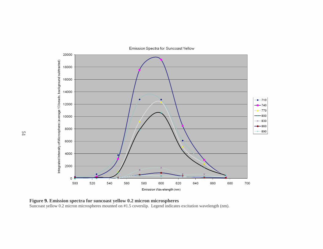
Figure 9. Emission spectra for suncoast yellow 0.2 micron microspheres Suncoast yellow 0.2 micron microspheres mounted on #1.5 coverslip. Legend indicates excitation wavelength (nm).
51
52
emission wavelengths measured. Figure 9 shows the emission spectra for suncoast
yellow with peak emission wavelengths in the range of 575-600 nm for all excitation
wavelengths. However for our studies, we used an excitation wavelength of 800 nm
because 740 nm excitation caused extremely fast photobleaching (data not shown) and
would have required such low laser power, it would have required additional optics to
attenuate the laser enough to measure the fluorescence saturation curve.
C. Effects from the media at the coverslip
The fluorescence intensity of 0.2 microns microspheres at the coverslip-sample
interface was compared for samples with different refractive index to investigate possible
effects from the sucrose solutions on fluorescence intensity. Figure 10 shows that
increasing sucrose concentration not only increased refractive index but also caused
immediate decrease in fluorescence at the surface of the sample. Therefore to assess
signal attenuation, fluorescence intensity data were normalized to the intensity at the
surface of the sample.
D. Fluorescence saturation
Fluorescence saturation was measured for suncoast yellow labeled 0.2 micron
microspheres. The fluorescence intensity of microsphere dried on the coverslip and
mounted with a 1.342 agarose sample was measured for laser powers ranging from 12.5-
60 mW after each realignment of the excitation path (Figures 11-13). Fluorescence
saturation was found to occur after 30 mW of excitation power, measured at the Pockels
cell. Therefore, 30 mW was the excitation power used for our studies.

53
Figure 10. Comparison of fluorescence intensity at the coverslip-sample interface for samples with different refractive index Fluorescence intensity was measured at the coverslip-sample interface for samples with different refractive index.
0
500
1000
1500
2000
2500
Mounting Refractive Index
Fluo
resc
ence
Inte
nsit
y (a
u)
1.3334
1.36408
1.39926
1.4397

54
Figure 11. Fluorescence saturation data Fluorescence saturation measured after excitation light path alignment before the signal attenuation study. Suncoast yellow 0.2 micron microspheres mounted on #1.5 coverslip. Each data point represents 50 microspheres collected in five images. Linear fit of data for the first 30 mW. Data collected with 800nm excitation wavelength, 600V detector gain, and XY pixel dimensions of 0.207um.

55
Figure 12. Fluorescence saturation data Fluorescence saturation measured after excitation light path alignment before the excitation attenuation study without DABCO. Suncoast yellow 0.2 micron microspheres mounted on #1.5 coverslip. Laser power was measured at the Pockels cell. Data collected with 800nm excitation wavelength and 0.101 micron XY pixel dimensions. A) Each data point represents three images with 4-13 microspheres. Data collected with 540V detector gain. Linear fit of data for the first 30 mW. B) Each data point represents three images with 3-15 microspheres. Data collected with 640V detector gain. Linear fit of data for the first 30 mW.

56
Figure 13. Fluorescence saturation data Fluorescence saturation measured after excitation light path alignment before the excitation attenuation study with DABCO. Suncoast yellow 0.2 micron microspheres mounted on #1.5 coverslip. Laser power was measured at the Pockels cell. Data collected with 800nm excitation wavelength, 535V detector gain, and 0.101 micron XY pixel dimensions. Linear fit of data for the first 30 mW. A) Each data point represents three images with 4-25 microspheres. B) Each data point represents three images with 4-14 microspheres. C) Each data point represents three images with 5-20 microspheres.

57
E. Signal attenuation
Since two-photon fluorescence excitation is quadratically related to photon
density, spherical aberration would be expected to diminish fluorescence excitation at
depth into refractive index mismatched samples. In order to isolate the effects of
spherical aberration on multiphoton fluorescence excitation, test samples were prepared
with minimal light scattering and absorption to assess the effects of refractive index
mismatch between the immersion medium, coverslip, and sample. Fluorescent
microspheres were suspended in samples of agarose, prepared with different refractive
indices using sucrose solutions. Images were collected with a 60x oil immersion
objective NA 1.4. The average intensity of the microspheres located at the coverslip was
calculated and used to normalize the data. Data from the individual microspheres at the
coverslip are not plotted to improve visualization because among the 12 trials there are
597 individual microspheres at the surface of the samples (Figure 14). The error for the
normalization of the data at the coverslip was calculated to be 2 % for each of the four
samples.
In all cases fluorescence intensity decreased with depth. However, as expected,
fluorescence intensity did not decrease as quickly in samples with refractive index closer
to the refractive index of the immersion oil, 1.515. In fact, at 40 microns deep into the
sample there is a 3.5-fold improvement in fluorescence signal in a sample with refractive
index 1.442 compared to a sample with refractive index 1.342.
Refractive index mismatch not only broadens the focal point, but it also causes a
focal shift [132]. In all samples, because the refractive index is less than that of the
immersion oil, the focal point will be increasingly offset toward the coverslip with depth

58
Figure 14. Fluorescence signal attenuation Fluorescence intensity of 0.2 micron microspheres mounted in agarose with varying refractive index, normalized to the average intensity at the surface, versus NFP. Images collected with 60x oil immersion objective NA 1.4 with immersion oil (refractive index 1.515). Lines represent the average of data from 25 microspheres per bin. Bin widths varied from 0.61 to 8.00 microns wide. Inset: Average normalized fluorescence intensity versus depth, where depth has been scaled using the paraxial approximation.

59
into the sample. In samples with refractive index 1.342, this offset is larger than in
samples with refractive index 1.442. Therefore the NFP, the measurement of depth based
on the physical movement of the stage, overestimates the AFP. By scaling depth using a
paraxial approximation, the ratio of the refractive index of the sample to the refractive
index of the immersion oil [133], the effect of refractive index mismatch on signal
becomes even more pronounced (Figure 14-Inset). Using the paraxial approximation to
scale imaging depth, at 40 microns deep into a sample with refractive index 1.442, there
is a 3.9-fold improvement in fluorescence signal over a sample with refractive index
1.342.
F. Resolution degradation
The effects of spherical aberration on resolution are hard to predict knowing that
decreased photon flux leads to decreased excitation. Axial resolution was measured as
the FWHM of the intensity distributed axially through the centroid of point spread
functions of sub-resolution microspheres mounted in agarose samples. At the surface of
the samples the axial resolution was measured with standard error to be 0.893 ± 0.005,
0.908 ± 0.006, 0.870 ± 0.014, and 0.928 ± 0.005 microns (mean ± standard error) for the
samples with refractive index 1.342, 1.371, 1.404, and 1.442 respectively. Data from
individual microspheres at the coverslip are not plotted to improve visualization, only the
average FWHM (Figure 15).
In all cases axial resolution degrades with imaging depth. However, the effect of
depth on resolution is less pronounced in samples whose refractive index is closer to that
of the immersion oil. Axial resolution degrades to 1.7 microns, nearly two-fold worse, at

60
Figure 15. Axial resolution degradation Axial intensity distribution FWHM of 0.2 micron fluorescent microspheres mounted in agarose with varying refractive index versus NFP. Images collected with 60x oil immersion objective NA 1.4 with immersion oil (refractive index 1.515). Lines represent the average of data from 30 microspheres per bin. Bin widths varied from 0.65 to 8.11 microns wide.

61
100 microns of depth into the sample with refractive index 1.442 but in less than 30
microns of depth into the sample with refractive index 1.342. At 100 microns deep into
the sample with refractive index 1.342, axial resolution is 2.5 microns, nearly 3-fold
worse than at the surface.
G. Excitation attenuation
1. Photobleaching rate
Because MPM relies on a multiphoton process, fluorescence excitation is highly
dependent on photon density. Therefore, we expect the preponderance of the signal
attenuation with depth in a refractive index mismatched sample to result from decreased
fluorescence excitation with depth. Since it is not possible to directly measure the rate of
fluorescence excitation, the effect of refractive index mismatch between the immersion
medium, coverslip, and sample on two-photon excitation was assessed indirectly by
measuring the effect of depth on photobleaching rates, which do not depend on
fluorescence collection, only fluorescence excitation. Quantification of the rate of
photobleaching of fluorescent microspheres mounted in agarose samples showed that
photobleaching rates decreased with imaging depth (Figure 16). However, the rate of
photobleaching at depth was higher in samples with refractive index closer to that of the
immersion oil. At 30 microns, the sample with refractive index 1.442 had over 7-fold
greater photobleaching than the sample with refractive index 1.342. The increase in
photobleaching rate at depth indicates that refractive index mismatch markedly affects
fluorescence excitation.

62
Figure 16. Photobleaching rate attenuation Photobleaching rate normalized at the surface of the sample versus NFP. Images were collected with 60x oil immersion objective NA 1.4 with immersion oil (refractive index 1.515) for five minutes of 0.2 micron fluorescent microspheres mounted in agarose samples with varying refractive index. Photobleaching rate was calculated for the average of 10-15 microspheres in 5 micron intervals and normalized to the photobleaching rate at the surface. Error bars represent standard deviation of three trials.
63
2. Excitation power versus photobleaching rate
Photobleaching data were measured at the coverslip-sample interface for different
laser powers to develop a calibration curve to convert photobleaching data to
fluorescence excitation power (Figure 17). Excitation intensity data could then be
compared directly to data calculated from a geometrical model of excitation intensity
distribution. And by squaring the excitation intensity data to predict fluorescence
excitation, we are able to compare these values with measured fluorescence signal to
calculate fluorescence emission attenuation at depth.
We found that the photobleaching rate of suncoast yellow label microspheres is
5.2-power of excitation which is very different from the intensity-squared dependence of
fluorescence excitation. Similarly, Patterson and Piston [127] measured photobleaching
rates of different fluorophores and found them to depend on ≥ 3 power of the excitation
intensity, with aminocoumarin dextran as high as 5.1 ± 0.2.
H. Emission attenuation
1. Fluorescence signal versus fluorescence excitation
On first principles, signal attenuation with depth is caused by attenuation of
fluorescence excitation and decreased collection efficiency of fluorescent emissions.
Based on the measurements of signal attenuation and excitation attenuation with depth,
the contribution of emission attenuation can be inferred. Excitation attenuation is shown
to be the predominant contributor to signal attenuation (Figure 18). At 40 microns deep
into the sample, only 20% of fluorescence is excited compared to fluorescence excitation

64
Figure 17. Calibration data Photobleaching data were collected of 0.2 micron fluorescent microspheres dried on the coverslip mounted with agarose sample with 2% DABCO and refractive index 1.342. Data were collected for laser powers measured at the Pockels cell in the range of 12.5-30mW. Images were collected with an Olympus 60x oil immersion objective NA 1.4.

65
Figure 18. Emission attenuation Signal attenuation and excitation attenuation versus NFP measured in agarose samples with refractive index 1.342 using a 60x oil immersion objective NA 1.4 with immersion oil (refractive index 1.515). Signal attenuation data are the average of data from 20 microspheres centered every five microns deep and normalized to the average fluorescence intensity at the surface. Excitation attenuation data are calculated from the photobleaching rates every five microns deep. Calculated fluorescence emission collection attenuation versus NFP calculated every five microns deep.

66
at the surface of the sample. Therefore, fluorescence excitation is attenuated by nearly
80%. However 40% of fluorescence emissions were collected at 40 microns deep into
the sample compared to collection at the surface of the sample. Therefore, collection of
emissions is attenuated by only about 60%.
2. Comparison of descanned and non-descanned detectors
Non-descanned detectors have been shown to improve collection of scattered
light, reducing the excitation power and detector gain necessary to generate bright images
[116]. To assess how signal attenuation with depth compares between non-descanned
and descanned detectors, image volumes were collected of agarose samples, refractive
index 1.34 (Figure 19). At 50 microns in depth, signal attenuated by 92%, using non-
descanned detectors, and by 95%, using the descanned detectors with the pinhole open
fully. Therefore although non-descanned detectors collect over 60% more scattered light
at 50 microns deep than descanned detectors, that only amounts to 3% more signal at 50
microns in depth.
I. Signal attenuation in kidney tissue
1. Comparison of agarose and kidney tissue samples
Images were collected of kidney tissue mounted in PBS, with refractive index
1.34, using an oil immersion objective. The rate of signal attenuation with depth into
kidney tissue was compared to that found in an agarose sample with refractive index
1.342 (Figure 20). Spherical aberration was shown to cause 88% of signal to attenuate at
30 microns deep in a sample with refractive index 1.342. In fixed kidney tissue mounted
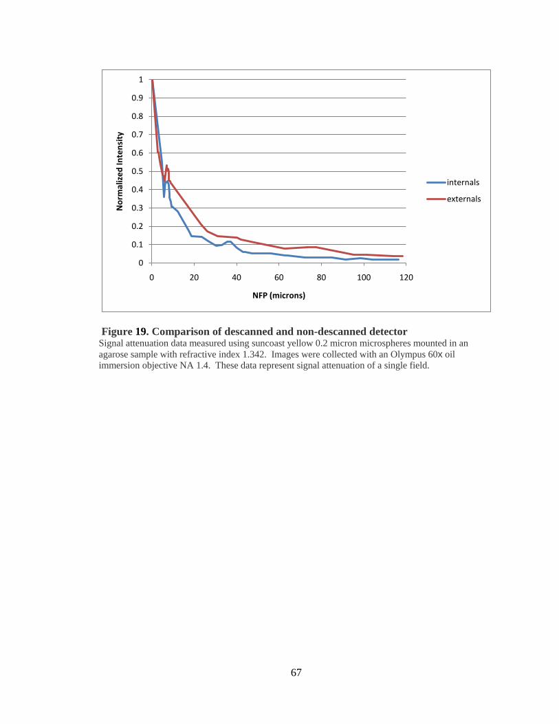
67
Figure 19. Comparison of descanned and non-descanned detector Signal attenuation data measured using suncoast yellow 0.2 micron microspheres mounted in an agarose sample with refractive index 1.342. Images were collected with an Olympus 60x oil immersion objective NA 1.4. These data represent signal attenuation of a single field.
0
0.1
0.2
0.3
0.4
0.5
0.6
0.7
0.8
0.9
1
0 20 40 60 80 100 120
Nor
mal
ized
Inte
nsit
y
NFP (microns)
internals
externals

68
Figure 20. Signal attenuation in kidney tissue Signal attenuation versus NFP of 0.2 micron fluorescent microspheres mounted in agarose with refractive index 1.404 or kidney tissue. Images were collected with a 60x oil immersion objective NA 1.4 with immersion oil (refractive index 1.515). The average of data from 20 microspheres are centered every five microns deep and normalized to the average fluorescence intensity at the surface. Error bars indicate the bin width and standard error.

69
in PBS, refractive index 1.34, signal attenuated by 98% at 30 microns deep, indicating
82% more signal attenuated that was not due to spherical aberration and was likely due to
scattering.
2. Comparison of water and oil immersion objectives
By collecting images with a water immersion objective, refractive index
mismatch between the immersion fluid, coverslip, and sample is reduced, decreasing the
effect of spherical aberration (Figure 21). Signal is significantly improved in the first 25
microns of depth; however, by 40 microns deep the improvement is negligible.

70
Figure 21. Water immersion objective versus oil immersion objective Signal attenuation of 0.2 micron fluorescent microspheres mounted in kidney tissue. Images were collected with a 60x oil immersion objective NA 1.4 with immersion oil (refractive index 1.515) or a 60x water immersion objective NA 1.2 with immersion water (refractive index 1.33). The average of data from 20 microspheres are centered every five microns deep and normalized to the average fluorescence intensity at the surface. Error bars indicate the bin width and standard error. Bin widths varied from 2.07 to 6.10 microns wide for data collected with the oil immersion objective and 1.71 to 11.68 microns wide for data collected with the water immersion objective.

71
Chapter 2. The effect of refractive index heterogeneity in multiphoton microscopy of
kidney tissue
A. The effect of mounting media refractive index on signal attenuation with depth in
kidney tissue using a water immersion objective
In order to evaluate the effect of the refractive index of mounting media on MPM
of biological tissues, we collected image volumes of kidney tissue labeled with Lens
Culinaris Agglutinin-Fluorescein and mounted in a set of clearing solutions with different
refractive indices. Figure 22 shows a series of XZ cross-sectional images of kidney
tissues mounted in different refractive index media collected with an Olympus 60x, NA
1.2 water immersion objective. Interestingly, the greatest depth was achieved in the
samples mounted in the highest refractive index media, refractive index 1.51 and 1.53.
This is surprising in that these samples should show the greatest amount of spherical
aberration, resulting from the greatest refractive index mismatch between the immersion
fluid and sample.
In order to quantify the effect of the refractive index of the mounting medium on
the rate of signal attenuation with depth, we collected images of 0.2 micron fluorescent
microspheres within kidney tissue mounted in media with refractive index 1.34, 1.40, or
1.51. Images were collected using an Olympus 60x NA 1.2 water immersion objective.
The average intensity of the microspheres located at the coverslip was calculated and
used to normalize the data. Data from the individual microspheres at the coverslip are
not plotted to improve visualization because among the 9 trials there are 365 individual

72
Figure 22. Qualitative study of signal attenuation caused by refractive index heterogeneity using water immersion objective Two-photon microscopy XZ cross-sectional images of kidney tissue mounted in media with refractive index 1.34, 1.40, 1.47, 1.48, 1.51, 1.53 and collected with an Olympus NA 1.2 water immersion objective. Pixel dimensions are 0.345x0.35 microns. Scale bar is 10 microns. Images collected by Sherry Clendenon.

73
microspheres at the surface of the samples. The standard error for the data at the
coverslip was calculated to be 1-3% for each of the three samples.
Quantization of microsphere fluorescence showed that, as in Figure 22, signal
levels attenuated most rapidly in the sample mounted in a medium of low refractive index
(Figure 23). For example, signal attenuated by 90% over an axial distance of 75 microns
in kidney tissue with refractive index 1.51, but the same degree of attenuation was seen
over only one third of this distance in a sample with refractive index 1.34. Thus, despite
an increase in refractive index mismatch, signal improved with depth, in agreement with
the images shown in Figure 22. This effect most likely resulted from a reduction in
refractive index heterogeneity. Interestingly in Figure 23, maximum fluorescence
intensity was not at the surface for all samples. Though this effect was outside the scope
of our study, this may have resulted from the extra lens elements used in the correction
collar of the water immersion objective.
Based upon refractive index mismatch, we expected that fluorescence intensity
would attenuate most rapidly in samples mounted in media with higher refractive index.
We previously found that refractive index mismatch compromised the achievable
imaging depth. Interestingly, we get better depth penetration with high refractive index
samples.
B. The effect of mounting media refractive index on resolution degradation with
depth in kidney tissue using a water immersion objective
Although we get better depth penetration with high refractive index samples, the
axial resolution is lower, as indicated by an increase in the axial FWHM of the intensity

74
Figure 23. Quantitative study of signal attenuation caused by refractive index heterogeneity using water immersion objective Two-photon microscopy of 0.2 micron fluorescent microspheres in kidney tissue mounted in media with refractive index 1.34, 1.40, or 1.51 and collected with an Olympus 60x NA 1.2 water immersion objective, refractive index 1.33. Line represents the average of data from 30 microspheres per bin. Bin widths varied from 2.34 to 13.42 microns wide.

75
profile on injected microspheres (Figure 24). Data from individual microspheres at the
coverslip are again not plotted to improve visualization, only the average FWHM at the
surface calculated for each sample with a standard error of 0.006-0.009 microns.
Samples mounted in media with refractive index 1.34 maintained axial resolution
on the order of 1 micron up to 40 microns deep into tissue; whereas, the axial resolution
of samples mounted in media with refractive index 1.51 was measured to be
approximately 1.5 and 2.0 microns at depths of 40 and 80 microns, respectively. This is
likely because scatter reduces illumination density but does not broaden it so much since
scattered illumination photons are discarded from the illumination spot. So, unlike
spherical aberration, scattering affects imaging depth by reducing the number of photons
reaching the focus, but not really affecting the effective volume of excitation.
C. The effect of reducing both and refractive index heterogeneity and mismatch on
signal attenuation with depth in kidney tissue
Based upon previous results, ideally we would eliminate refractive index
mismatch and scattering. In order to evaluate the effect of simultaneously reducing both,
we collected images of kidney tissue labeled with Lens Culinaris Agglutinin-Fluorescein
and mounted in various media, using an oil immersion objective. To minimize scattering
and spherical aberration, the kidney tissue was mounted in different clearing solutions,
and XZ cross-sectional images were collected using an Olympus 60x NA 1.4 oil
immersion objective. The deepest imaging depth was achieved in the samples mounted
in refractive index media 1.51, clearing the tissue and matching the refractive index of the
immersion oil (Figure 25).

76
Figure 24. Quantitative study of resolution degradation caused by refractive index heterogeneity using water immersion objective Two-photon microscopy of 0.2 micron fluorescent microspheres in kidney tissue mounted in media with refractive index 1.34, 1.40, or 1.51 and collected with an Olympus 60x NA 1.2 water immersion objective, refractive index 1.33. Line represents the average of data from 31 microspheres per bin. Bin widths varied from 2.50 to 19.86 microns wide (excluding the deepest bins for each sample the maximum bin width was 8.30 microns wide).
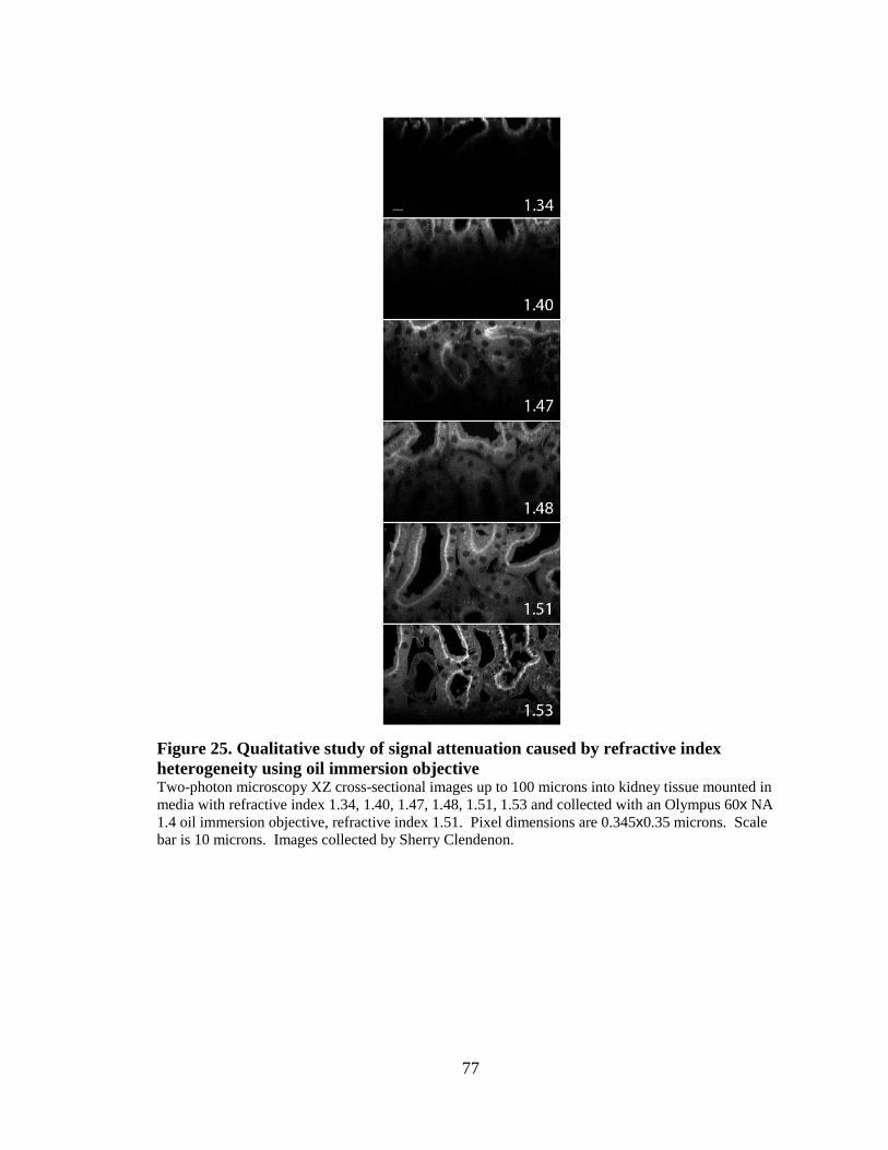
77
Figure 25. Qualitative study of signal attenuation caused by refractive index heterogeneity using oil immersion objective Two-photon microscopy XZ cross-sectional images up to 100 microns into kidney tissue mounted in media with refractive index 1.34, 1.40, 1.47, 1.48, 1.51, 1.53 and collected with an Olympus 60x NA 1.4 oil immersion objective, refractive index 1.51. Pixel dimensions are 0.345x0.35 microns. Scale bar is 10 microns. Images collected by Sherry Clendenon.

78
These qualitative results were supported in quantitative analyses of fluorescent
microspheres in kidney tissue. Samples were mounted in media with refractive indices of
1.34, 1.40, or 1.51 and imaged using an Olympus 60x NA 1.4 oil immersion objective
(refractive index of the immersion oil, 1.515). The average intensity of the microspheres
located at the coverslip was calculated and used to normalize the data. Data from the
individual microspheres at the coverslip are not plotted to improve visualization because
among the 9 trials there are 456 individual microspheres at the surface of the samples.
The standard error for the data at the coverslip was calculated to be 1-2% for each of the
three samples.
As shown in Figure 26, the rate of signal attenuation with depth was dramatically
decreased in samples mounted in a high refractive index medium. Signal attenuated by
90% in less than 20 microns of depth into kidney tissue mounted in medium with
refractive index 1.34, whereas in samples mounted in medium with refractive index 1.51
signal only attenuated by 45% in 100 microns of depth. There results support the notion
that scattering of the excitation and fluorescent light, and not spherical aberration, is a
major contributor to signal degradation under our experimental conditions.
Remarkable results were obtained in samples mounted in the highest refractive
index media (Figure 27). High quality images were collected through the entire working
distance of the objective, 150 microns. Interestingly, even though scattering has been
significantly reduced, the shortest wavelength emissions still attenuate faster with depth
than the longer wavelengths. This is evident from the Figure 27C, 125 microns deep into
tissue, which has far more red signal (emission wavelengths 560-650 nm), than Figure
27A, 25 microns deep into tissue, which has far more blue signal (emission wavelengths

79
Figure 26. Quantitative study of signal attenuation caused by refractive index heterogeneity using oil immersion objective Two-photon microscopy of 0.2 micron fluorescent microspheres in kidney tissue mounted in media with refractive index 1.34, 1.40, or 1.51 and collected with an Olympus 60x NA 1.4 oil immersion objective, refractive index 1.515. Line represents the average of data from 25 microspheres per bin. Bin widths varied from 1.30 to 11.29 microns wide.

80
Figure 27. Optimization of refractive index heterogeneity and mismatch Two-photon microscopy of kidney tissue labeled with Hoechst, Lens Culinaris Agglutinin-Fluorescein, and Phalloidin-Rhodamine and mounted in media with refractive index 1.51. Image volume collected with Olympus 60x NA 1.4 oil immersion objective. Images were collected A) 25 microns deep, B) 75 microns deep, C) 125 microns deep, and D) XZ cross-section. Pixel dimensions are 0.414x0.414x0.41 microns. Scale bar is 10 microns. Contrast stretching and unsharp mask were the same for all images. Images collected by Sherry Clendenon.

81
380-480 nm). This is also evident in Figure 27D, XZ cross-section, with more blue
signal near the surface and red signal at depth.
D. The effect of reducing both and refractive index heterogeneity and mismatch on
resolution degradation with depth in kidney tissue
Our previous studies demonstrate that refractive index mismatch compromises
axial resolution in images collected at depth by MPM. Consistent with this observation,
increasing the refractive index of the mounting medium to match that of the immersion
medium profoundly improved the axial resolution of images of microspheres collected at
depth in kidney tissue (Figure 28). Data from individual microspheres at the coverslip
are again not plotted to improve visualization, only the average FWHM at the surface
calculated for each sample with a standard error of 0.003-0.006 microns.
Quantitative analysis of microsphere point spread functions in these samples
demonstrates that eliminating refractive index mismatch essentially eliminates depth-
induced degradation in axial resolution. The axial resolution of samples mounted in
media with refractive index 1.34 was measured to be approximately 1.5 microns 25
microns deep into tissue. Samples mounted in media with refractive index 1.51
maintained axial resolution on the order of 0.9 microns up to 100 microns deep into
tissue.
The results of these studies demonstrate that additional profound improvement in
reach and image quality can be achieved by minimizing spherical aberration and
scattering.

82
Figure 28. Quantitative study of resolution degradation caused by refractive index heterogeneity using oil immersion objective Two-photon microscopy of 0.2 micron fluorescent microspheres in kidney tissue mounted in media with refractive index 1.34, 1.40, or 1.51 and collected with an Olympus 60x NA 1.4 oil immersion objective, refractive index 1.515. Line represents the average of data from 40 microspheres per bin. Bin widths varied from 3.38 to 10.94 microns wide.

83
Chapter 3. Mathematical model of refractive index mismatch in MPM using
geometric optics
A. Theory
A mathematical model was developed using geometrical optics to predict the
excitation light path from the objective lens to the focus through the immersion fluid,
coverslip, and into a homogeneous sample. This geometrical model is used to calculate
the first order approximation of the axial distribution of excitation and fluorescence
intensity demonstrating the effect of refractive index mismatch in multiphoton
fluorescence microscopy.
This geometrical model relies on Snell’s law which states
𝑛1𝑠𝑖𝑛 𝛼1 = 𝑛2𝑠𝑖𝑛 𝛼2
where 𝑛1 is the refractive index of the first medium, 𝛼1 is the angle of incidence, 𝑛2 is the
refractive index of the second medium, and 𝛼2 is the angle of refraction. Using Snell’s
law and the objective lens parameters for an Olympus 60x NA 1.4 oil immersion
objective lens (PLAPO60XO3) (Table 3), we calculate initial parameters (Figure 29).
By definition
𝑁𝐴 = 𝑛𝑜𝑏𝑗 sin𝛼𝑁𝐴
where 𝑁𝐴 is the numerical aperture of the objective lens, 𝑛𝑜𝑏𝑗 is the ideal refractive
index as described by the objective manufacturer, and 𝛼𝑁𝐴 is the aperture angle of the
objective lens. By simple geometry
𝑟𝑚𝑎𝑥 = 𝐴 tan𝛼𝑁𝐴

Objective lens parameters
numerical aperture 𝑁𝐴 1.4 ideal refractive index 𝑛𝑜𝑏𝑗 1.515 working distance + ideal coverslip thickness (microns) 𝐴 150 microns + 170 microns = 320 actual refractive index of objective lens 𝑛 1.51633
Table 3. Objective lens parameters Objective lens parameters for an Olympus 60x NA 1.4 oil immersion objective lens (PLAPO60XO3).
84

85
Figure 29. Model schematic Using the objective parameters: numerical aperture, 𝑁𝐴, ideal objective refractive index 𝑛𝑜𝑏𝑗, working distance + ideal coverslip thickness, 𝐴, and actual objective lens refractive index, 𝑛, we calculate the maximum radius of incident light at the objective, 𝑟𝑚𝑎𝑥, the aperture angle, 𝛼𝑁𝐴, the angle of light from radius, 𝑟, assuming no refraction, 𝛼(𝑟), and the actual angle of light from radius, 𝑟, incident on the objective lens, β(r).

86
where 𝑟𝑚𝑎𝑥 is the maximum radius of incident light at the objective, 𝐴 is the sum of the
working distance and the ideal coverslip thickness, and 𝛼𝑁𝐴 is the aperture angle of the
objective lens (Figure 29). And assuming no refraction, the angle of light from radius, 𝑟,
can be defined as
𝛼(𝑟) = tan−1𝑟𝐴
where 𝐴 is the sum of the working distance and the ideal coverslip thickness (Figure 29).
However, because the actual refractive index of the objective lens is not the ideal
refractive index indicated by the manufacturer for the immersion fluid of the system, we
use Snell’s law to define the actual angle of light incident on the objective lens
𝑛 sin𝛽(𝑟) = 𝑛𝑜𝑏𝑗 sin𝛼(𝑟)
where 𝑛 is the actual refractive index of the objective lens and 𝑛𝑜𝑏𝑗 is the ideal refractive
index as described by the objective manufacturer (Figure 29). Using 𝑛 and 𝛽(𝑟), we
define refraction angles 𝜃1, 𝜃2, and 𝜃3 for the objective lens-immersion fluid interface,
immersion fluid-coverslip interface, and coverslip-sample interface respectively
𝑛 sin𝛽(𝑟) = 𝑛1 sin𝜃1(𝑟) = 𝑛2 sin𝜃2(𝑟) = 𝑛3 sin𝜃3(𝑟)
where 𝑛1 is the refractive index of the immersion fluid, 𝑛2 is the refractive index of the
cover glass, and 𝑛3 is the refractive index of the sample (Figure 30). We calculate the
depth into the sample, 𝑍(𝑟), where light from a cone with radius, 𝑟, will focus
𝑍(𝑟) =𝑟 − 𝐷 tan𝜃1(𝑟) − 𝑇 tan𝜃2(𝑟)
tan 𝜃3(𝑟)
where 𝐷 is the distance from the objective lens to the coverslip and 𝑇 is the coverslip
thickness. Using this calculation and radially stepping across the objective lens from

87
Figure 30. Model schematic Using 𝛽(𝑟) calculated from the objective parameters, for light from a specific radius, 𝑟, we calculate refraction angles, 𝜃1(𝑟), 𝜃2(𝑟), and 𝜃3(𝑟), for refractive indices, 𝑛1, 𝑛2, and 𝑛3, respectively, chosen based on values from actual experiments. Using the refraction angles, 𝜃1(𝑟), 𝜃2(𝑟), and 𝜃3(𝑟), we can calculate the depth into the sample from the coverslip-sample interface that light from a specific radius, 𝑟, focuses.

88
paraxial rays to peripheral rays, we are able to build a linear projection histogram
representing the distribution of excitation intensity axially within the sample.
However, because we are modeling excitation intensity for a 0.2 micron diameter
fluorescent microsphere, confining the focal spot to a single point is unreasonable. It is
necessary to consider all rays that pass within the volume of the microsphere. Also, we
know diffraction causes the focus to have an intensity distribution, PSF, with FWHM of
0.3 microns laterally and 0.9 microns axially at an excitation wavelength of 800 nm using
a 60x oil immersion objective NA 1.4. Therefore, to determine the excitation intensity
within the sample for a specific 𝐷 and 𝑇, we sum the intensities from cones of light that
focus within a range of a certain depth, 𝑍𝑓𝑝.
To determine the excitation intensity for a given 𝑍𝑓𝑝, we integrate the input laser
beam intensity over 𝑟 such that the excitation light passes within a range of 𝑍𝑓𝑝 (Figure
31)
∫ 𝐼(𝑟)𝑑𝑟.
The axial range is defined such that 𝑍(𝑟) is bound by
𝑍𝑓𝑝 − 𝑦 ≤ 𝑍(𝑟) ≤ 𝑍𝑓𝑝 + 𝑦 .
The lateral range is defined such that 𝑍(𝑟) and tan𝜃3(𝑟) are bound by
�𝑍(𝑟) − 𝑍𝑓𝑝� tan𝜃3(𝑟) ≤ 𝑥 .
Although we are using geometrical optics to model our system, we model the input light
as a Gaussian beam with a cylindrically symmetric wavefront using the beam radius and
average power measured at the back aperture of the objective.

Figure 31. Model Schematic The intensity for light rays focusing within an axial and lateral range of 𝑍𝑓𝑝 is summed to determine the excitation intensity.
A B
89

90
Using a Gaussian distribution for intensity yields
𝐼(𝑆) =2𝑃0𝜋𝑤2 𝑒
−2𝑆2𝑤2
where 𝑃0 is the average power at the back aperture of the objective and 𝑤 is the beam
radius of the laser at the back aperture (Figure 32). The microscope objective is
simplified to two lenses, the objective lens and a lens at the back aperture. The back
aperture lens is idealized to take on all the properties of the lenses within the microscope
objective such that light at the back aperture projects on to the objective lens with angle
𝛽(𝑟). The back aperture is assumed to be filled, which refers to the FWHM of the
Gaussian beam equaling the diameter of the back aperture of the microscope objective.
Therefore the beam radius, 𝑤, measured as half the FWHM of the Gaussian beam, equals
the radius of the back aperture of the objective.
Assuming cylindrical symmetry, the excitation intensity integral becomes
𝐼 = �2𝑃0𝜋𝑤2 𝑒
−2𝑆2
𝑤2 (2𝜋𝑆)𝑑𝑆𝑆2
𝑆1
where 𝑆1 and 𝑆2 are determined using MATLAB (The MathWorks, Inc., Natick, MA,
USA) to iterate over 𝑟, calculating 𝑆1 from 𝑟 when it first encounter a ray within the axial
or lateral range of 𝑍𝑓𝑝, and 𝑆2 when subsequently, 𝑟 encounters a ray that is no longer in
the axial or lateral range of 𝑍𝑓𝑝 (Figure 31). 𝑆 is calculated from 𝑟 by
𝑆(𝑟) = 𝑤−𝑟𝑚𝑎𝑥
tan�sin−1 NAn �tan𝛽(𝑟) + 𝑟.
This is repeated though 𝑟𝑚𝑎𝑥 summing intensities to get the total intensity at 𝑍𝑓𝑝.
To determine at what depth is the AFP for a particular 𝐷 and 𝑇, this is repeated by
iteratively stepping 𝑍𝑓𝑝 from the coverslip-sample interface
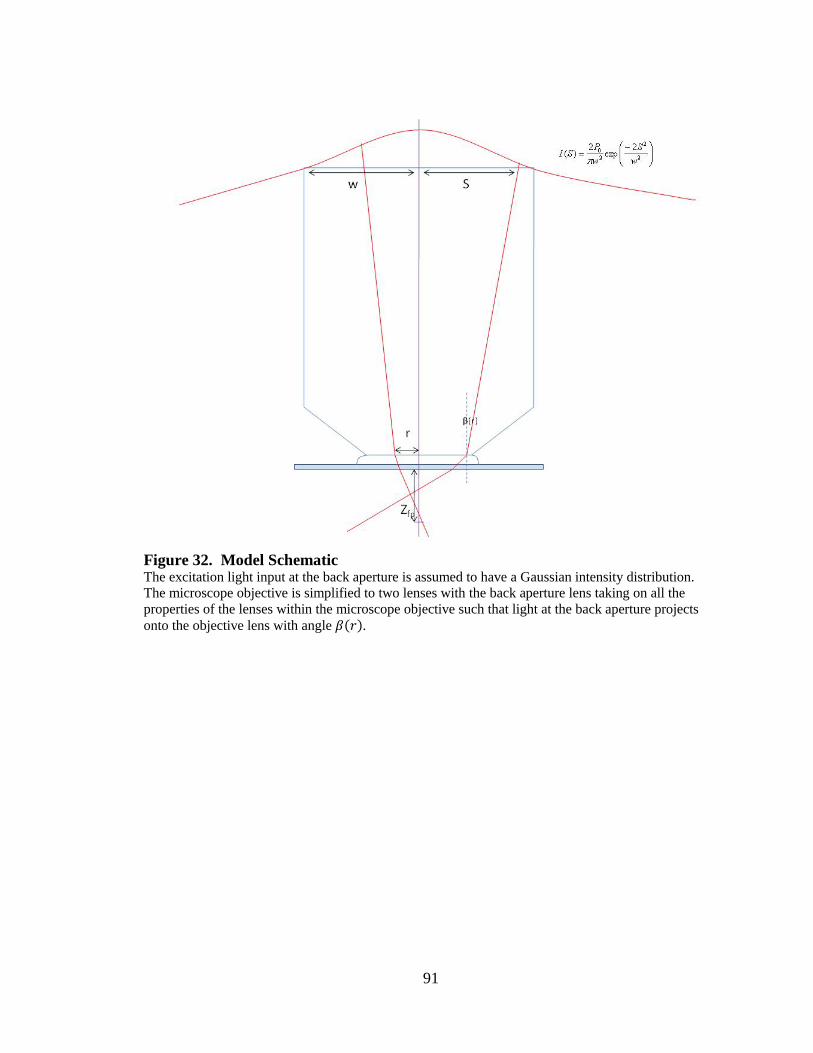
91
Figure 32. Model Schematic The excitation light input at the back aperture is assumed to have a Gaussian intensity distribution. The microscope objective is simplified to two lenses with the back aperture lens taking on all the properties of the lenses within the microscope objective such that light at the back aperture projects onto the objective lens with angle 𝛽(𝑟).

92
deep into the sample. The depth, 𝑍𝑓𝑝, where the maximum intensity is achieved is the
AFP for 𝐷 and 𝑇 (Figure 33). To compare to experimental data, this is repeated for 𝐷,
the distance from the coverslip to the objective lens, ranging through the full working
distance of the objective to find the maximum intensity associate with each step of the
objective, 𝐷. The NFP is
𝑁𝐹𝑃 = 𝐴 − (𝐷 + 𝑇).
B. MATLAB
1. Overview
Because the mathematical model could not be solved analytically, MATLAB
(The MathWorks, Inc., Natick, MA, USA) was used to calculate the excitation intensity
versus focal depth numerically. The code can be found in Appendix 1.
The Intensity program was written to calculate the excitation intensity for a given
AFP and distance between the objective and coverslip, D.
The Optimize D program was then written to find at what D, the distance between
the objective and coverslip, the maximum intensity occurs for a given AFP and sample
refractive index. The Optimize D program runs the Intensity program for all D through
the full working distance of the objective.
The Optimize D Range program finds the optimized D value, the associated
maximum intensity for a range of focal positions and a given sample refractive index.
The Optimize D Range program was run for focal positions from 1 micron to 149
microns, with a 1 micron step.

93
Figure 33. Model schematic The intensity for light rays focusing within a range of 𝑍𝑓𝑝 is summed to determine the excitation intensity. 𝑍𝑓𝑝 is iteratively stepped axially through the sample, to find the depth where the excitation intensity is maximal, the AFP.

94
The Overnight OD program produces saved files each containing a spreadsheet of
the full range of focal positions from 1-149, each associated optimized D, and the
associated maximum intensity. The Overnight OD program runs the Optimize D Range
program for each sample refractive index input into an array.
2. Intensity program
The program intensityford was developed to calculate the excitation intensity
at a specific focal plane. This program requires input values of d, the distance between
the coverslip and the objective, fp, the focal plane, and rstep, the step size to iterate
across the radius of the objective lens. This program steps across the radius of the
objective lens and determines if the associated ray of excitation light propagates within a
range of the focal plane, fp. This is determined using the function thetans, a
convenience function that performs calculations that occur in several places described
below. Using the values returned by thetans, the ray is tested to see if it propagates
within the range of fp (Figure 31). If it is within either the lateral range, lower <=
tan(theta3) and tan(theta3) <= upper, or the axial range, fp-.1 <= z and z <=
fp+.1, then the variable R1 is set equal to r. R1 is the first r position where a ray of
excitation light contributes to the excitation intensity at the focal plane, fp.
intensityford continues stepping r across the objective lens until it finds an r that is
not in bounds. It sets the previous r position equal to R2. R2 is the last r position where
a ray of excitation light contributes to the excitation intensity at the focal plane, fp.
Because we are assuming the excitation light has a Gaussian wavefront filling the back
aperture of the objective, the excitation intensity cannot be calculated directly from R1

95
and R2. Using the function S, described below, R1 and R2 are converted to S1 and S2, the
associated radii at the back aperture of the objective. S1 and S2 are then used to calculate
the integrated intensity from this ring of excitation as intensity = pi * w^2 / 2 *
abs(sintensity(S2) - sintensity(S1)). The function sintensity is described
below. Because there may be more rays of excitation light that contribute to the
excitation intensity farther along r, the function continues stepping r across the objective
lens until it reaches rmax. If it encounters another r position in bounds, it repeats and
adds the excitation intensity from this ring of light to the total intensity.
The function, thetans, performs calculations that occur in several places and
requires input values for r, the radius at the objective lens to be tested, and d and fp,
which are the original values inputted into intensityford. thetans calculates alphar,
beta, theta1, theta2, theta3, z, lower, and upper. alphar is the angle of light from
radius, r, assuming no refraction. beta is the actual angle of light incident on the
objective lens. theta1 is the refraction angle from the objective lens-immersion fluid
interface. theta2 is the refraction angle for the immersion fluid-coverslip interface.
theta3 is the refraction angle for the coverslip-sample interface. z is the depth into the
sample where light from a cone with radius, r, with focus. lower and upper are the
bounds associated with the lateral range around fp for a given radius r. thetans returns
beta, theta3, z, lower, and upper.
The function, S, calculates the radial position at the back aperture of the objective
associate with a value r, the radial position at the objective lens, and beta, the actual
angle of light incident on the objective lens calculated by the function thetans. This is
calculated using the equation sposition = (w - rmax) / (tan (asin (NA / N))) *

96
tan (beta) + r. w, rmax, NA, and N are global variables defined in Table 4. w is the
radius of the back aperture of the objective, rmax is the radius of the objective lens, NA is
the numerical aperture of the objective, and N is the actual refractive index of the
objective lens glass.
The function, sintensity, calculates the excitation intensity for a given radial
position along the back aperture of the objective, s, assuming a Gaussian wavefront.
This is calculated using the equation sint = I * exp(-2 * (s)^2 / (w^2)). I is the
intensity at the peak of the Gaussian distribution, a global variable defined in Table 4.
3. Optimize D program
The program, optimized, was developed to use the data from the
intensityford program to find the maximum intensity for the given focal plane and the
associated distance between the objective and the coverslip. The program, optimized,
requires input values fp, the focal plane, and ned, the refractive index of the sample. The
program runs intensityford for a range of d, the distance between the objective and
coverslip, through the full working distance of the objective, stepping at micron intervals.
The program, intensityford, returns the excitation intensity for a specific focal plane,
given a specific distance between the objective and coverslip. To find the maximum
intensity, optimized steps d through the working distance of the objective, running
intensityford using d, the given fp, and an rstep of 1. The variable maxintensity is
set equal to the intensity value returned by intensityford if the new intensity is greater
than the intensity for the previous d. This is repeated until the new intensity value is less
than maxintensity. Once the maximum intensity is found, this is repeated for a smaller
range of d, d ± 2, with a finer interval, where the step is reduced to a tenth of a micron.

97
Global variables NA 1.4 numerical aperture of the objective NOBJ 1.515 refractive index of the objective WOBJ 150 working distance of the objective in microns T 170 coverslip thickness in microns
WDT WOBJ+T working distance + ideal coverslip thickness in microns
N 1.51633 actual refractive index of the objective lens glass N1 1.515 refractive index of the immersion fluid N2 1.515 refractive index of the cover glass N3 ned refractive index of the sample ALPHA asin(NA/NOBJ) aperture angle rmax (WDT)*tan(ALPHA) radius of the objective lens
w 4200 radius of the back aperture in microns and beam radius
P 2000 power in microWatts I 2*P/(3.14159*w^2) intensity at the peak of the Gaussian delta 10^-58 fluorophore cross section in m^4sec f 82*10^6 repetition rate of laser in Hz tau 100*10^-15 temporal pulse width of laser in seconds lambda 800*10^-9 wavelength in meters X 0.1 lateral range to include at fp ZRANGE 150 distance from coverslip into the sample in microns
Table 4. Global variables Global variables used in geometrical model. Objective lens parameters based on an Olympus 60x NA 1.4 oil immersion objective lens (PLAPO60XO3).

98
This is again repeated with finer passes until the dstep is 0.0001 microns. Initially we
attempted using built-in minimization functions, but we ran into problems with local
minima and maxima. While a linear search is not idea or efficient, it is reliable.
optimized returns the distance between the objective and the coverslip where the
excitation intensity is a maximum found during this final search.
4. Optimize D Range program
The program, optimizedrange, was developed to find the maximum intensity
and associated distance between the objective and coverslip for a range of focal positions
and a given refractive index of the sample, ned. This program repeatedly runs
optimized for the range of focal positions from 1 micron deep into the sample through
ZRANGE - 1. Calculations are not defined at focal position 0 microns or when ZRANGE =
WOBJ. optimizedrange returns an array with three values, the focal position, fp, the
distance between the objective and the coverslip where the excitation intensity is a
maximum, returned from optimized, and the maximum intensity returned from
intensityford.
5. Overnight OD program
The program, overnightod, was developed to run optimizedrange for multiple
refractive indices of the sample input as an array, ned, and save the data in a separate
spreadsheet for each refractive index. overnightod iterates over the input array, ned,
and populates a spreadsheet with the focal position, fp, the distance between the
objective and the coverslip where the excitation intensity is a maximum, returned from
optimized, and the maximum intensity returned from intensityford.

99
6. Model calculations
Calculations from the model are presented in Figure 34 and 35. Figure 34 is a
plot of the maximum intensity returned from intensityford versus the AFP, fp. In
Figure 35 the maximum intensity data are normalized to the value at fp = 1 and are
plotted versus the NFP, calculated as the difference between the working distance of the
objective, WOBJ, and the distance between the objective and the coverslip where the
excitation intensity is a maximum, returned from optimized.
C. Comparison to empirical data
The geometrical model was developed to predict the excitation light path from the
objective lens to the focus through the immersion fluid, coverslip, and into a
homogeneous sample. This model is used to calculate the first order approximation of
the axial distribution of excitation intensity. Calculations made based on the geometrical
model were compared to the excitation attenuation data collected as described in
Excitation attenuation (Figure 36). Briefly, photobleaching rates were measured over a
range of depths in samples of agarose, a homogeneous sample, with refractive indices
1.34, 1.37, 1.40, 1.44 containing 0.2 micron fluorescent microspheres (Figure 16).
Photobleaching rates were also collected at the coverslip-sample interface for a range of
laser powers measured at the Pockels cell. A calibration curve was developed relating
photobleaching rates and laser power (Figure 17). The calibration curve was then used to
convert photobleaching rates versus depth to excitation power versus depth.
Model calculations and empirical data were normalized to the intensity five
microns deep into the sample because the model was undefined at the coverslip-sample

100
Figure 34. Model calculations The intensity for light rays focusing within a range of 𝑍𝑓𝑝 is summed to determine the excitation intensity. 𝑍𝑓𝑝 is iteratively stepped axially through the sample, to find the depth where the excitation intensity is maximal, the AFP. This is repeated for 𝐷, the distance from the coverslip to the objective lens, ranging through the full working distance of the objective to find the maximum intensity associate with each step of the objective, 𝐷. The maximal intensity is plotted versus AFP.

101
Figure 35. Model calculations The intensity for light rays focusing within a range of 𝑍𝑓𝑝 is summed to determine the excitation intensity. 𝑍𝑓𝑝 is iteratively stepped axially through the sample, to find the depth where the excitation intensity is maximal, the AFP. This is repeated for 𝐷, the distance from the coverslip to the objective lens, ranging through the full working distance of the objective to find the maximum intensity associate with each step of the objective, 𝐷. The NFP is calculated from 𝐷. The maximal intensity is normalized to the value at one micron below the coverslip-sample interface and is plotted versus NFP.

Figure 36. Comparison of model and empirical data The photobleaching data were converted to excitation attenuation using the calibration curve. Because the model was undefined for 𝑍𝑓𝑝 = 0, the model was calculated started at 𝑍𝑓𝑝 = 1 micron. Therefore both empirical data and model calculations were normalized to NFP = 5 microns.
102
103
interface. Because the model calculated a much faster attenuation rate than the
experimental data, this also improved agreement between the model and empirical data.
In fact, there is near agreement at depth for the 1.34 and 1.40 samples. However, overall
the model was not a good predictor of the experimental data.
Although squaring the excitation intensity will model two-photon fluorescence
excitation, signal attenuation data from Figure 14 were not compared to model
predictions because attenuation of fluorescent emissions were not modeled.

104
IV. DISCUSSION
A. Summary
In Chapter 1, refractive index mismatch was shown to result in a rapid
degradation of axial resolution, attenuation of signal and fluorescence excitation with
depth, even in samples lacking significant scattering or absorption. This is likely due to
spherical aberration-induced broadening of the focal point. In samples with reduced
mismatch in refractive index, fluorescence excitation, signal, and resolution were
improved.
In Chapter 2, we showed that refractive index heterogeneity in kidney tissue plays
a significant role in signal attenuation with depth in MPM. Since refractive index
heterogeneity causes scattering which has been shown to be a predominant cause of
signal attenuation with depth, we investigated a simple way to minimize scatter, which
profoundly improves image quality of deep tissue MPM images. Our clearing method
utilizes a benzyl alcohol and glycerol solution to raise the background refractive index of
kidney tissue, lowering the reduced scattering coefficient.
In Chapter 3, we modeled the effect of refractive index mismatch on fluorescence
intensity with depth in multiphoton fluorescence microscopy. We took a geometrical
optics approach, neglecting diffraction, to approximate to first order the axial distribution
of light intensity typically used to trigger a two-photon event in multiphoton microscopy
of biological tissue. However to improve the model, the excitation light was modeled as
a Gaussian beam with a cylindrically symmetric wavefront using the beam radius and
average power measured at the back aperture of the objective. Using this approach we

105
modeled how excitation intensity decreases due to refractive index mismatch between the
immersion fluid and sample as one focuses deeper into a sample. These findings will be
discussed in more detail below.
B. The effect of refractive index mismatch on signal attenuation
Refractive index mismatch between the immersion medium and sample causes
spherical aberration which widens the focus of illumination light, reducing the photon
density. Accordingly, studies in model systems have shown that spherical aberration
causes fluorescence signal to attenuate with depth in MPM [115, 131, 136-138]. As
expected, we found that fluorescence signal attenuated as a function of the magnitude of
refractive index mismatch. This is likely due to spherical aberration-induced broadening
of the focal point. In samples with reduced refractive index mismatch, fluorescence
signal at depth was improved.
We and others have shown that further improvement in reach can be
accomplished by manipulating spherical aberration via objective lens adjustment collars
[110, 111]. More elaborate, but still easily implemented solutions for correcting
spherical aberration in MPM include adaptive optics manipulations of the illumination
beam, which has been shown to effectively address a variety of tissue-induced
aberrations and thus improve the reach of MPM [138, 174, 175]. Unfortunately, adaptive
optics requires collection of many images to derive the solution that will correct for the
aberrations. This increases collection time, photobleaching, and photodamage. Time
resolution is extremely important for collection of images of dynamic processes;
therefore, current adaptive optics solutions are not well-suited for intravital imaging. Our

106
results suggest that, rather than using an exhaustive trial-and-error iterative approach,
significant improvement in image quality may be more rapidly obtained with mirror
solutions chosen from a much smaller subset of potential solutions directed at correcting
spherical aberration.
C. The effect of refractive index mismatch on excitation attenuation
By measuring photobleaching rates, we were able to examine the effect of
refractive index mismatch on excitation attenuation. The photobleaching rate depends on
fluorescence excitation, but not on collection efficiency. Therefore, by comparing
photobleaching rates at depth in samples with differing refractive indices, we showed that
samples with greater refractive index mismatch had slower photobleaching rates at depth
than those with less refractive index mismatch. These results indicate that greater
refractive index mismatch causes more rapid attenuation of fluorescence excitation in
MPM.
In principle, spherical aberration may reduce both excitation and collection of
fluorescence. However, based upon the quadratic dependence of fluorescence excitation,
and the use of non-descanned detectors, we anticipated that the preponderant effect of
spherical aberration would be to reduce fluorescence excitation. As expected, excitation
attenuation was shown to be the major contributor to signal attenuation with depth in
MPM. Using an oil immersion objective, fluorescence excitation attenuated by nearly
80% at 40 micron-depth in agarose samples with refractive index 1.342. This is likely
due to the quadratic dependence of fluorescence on excitation power when collecting

107
images with MPM. Therefore, optimizing fluorescence excitation as a function of depth
is key to improving MPM images at depth.
D. The effect of refractive index mismatch on emission attenuation
Although spherical aberration was shown to predominantly affect excitation
attenuation with depth in MPM, collection efficiency was also shown to depend on
spherical aberration. Using the measured signal attenuation and excitation attenuation,
we were able to calculate the fraction of fluorescence collected at depth compared to
fluorescence collected at the surface of the sample. It was shown that collected emissions
attenuated by 60% at 40 microns. Use of non-descanned detectors improves collection of
scattered light, reducing the excitation power and detector gain necessary to generate
bright images [116]. To assess how signal attenuation with depth compares between non-
descanned and descanned detectors, image volumes were collected of agarose samples,
refractive index 1.34. At 50 microns in depth, signal attenuated by 92%, using non-
descanned detectors, and by 95%, using the descanned detectors with the pinhole open
fully. Therefore although non-descanned detectors collect over 60% more scattered light
at 50 microns deep than descanned detectors, that only amounts to 3% more signal at 50
microns in depth. Therefore regardless of detection method, attenuation of collection
with depth is not nearly as important as attenuation of excitation.
E. Signal attenuation in kidney tissue
In order to assess the contribution of spherical aberration to signal attenuation in
kidney tissue, signal attenuation was compared in kidney tissue and homogeneous test

108
samples of agarose with refractive index of 1.342, which matches the refractive index of
the tissue mounting medium, PBS of 1.34. At 30 microns deep into the sample, signal
attenuated by 98% in kidney and attenuated by 88% in a sample largely lacking in
scattering and absorption, but similar in refractive index. Therefore, while a large
fraction of signal attenuation in kidney tissue could be attributed to refractive index
mismatch, an approximately equal further attenuation in signal (82%) was obtained in the
kidney sample, likely due to light scatter and absorption induced by the tissue.
By collecting images with the water immersion objective, which closely matches
the refractive index of kidney tissue mounted in PBS, fluorescent signal was greatly
improved over the first 25 microns into the sample. However, at depths greater than 25
microns, the benefit of matching refractive index decreased. Therefore although, by
comparing kidney tissue to test samples, it seemed that spherical aberration and scattering
contributed equally to signal attenuation, these data indicate that spherical aberration is
most significant at shallow depths while scattering is the predominant contributor further
into biological tissue. Nonetheless, we have shown that spherical aberration can be a
major contributor to depth-dependent signal attenuation in MPM, and that in fixed kidney
tissue, signal attenuation can be improved by use of a water immersion objective.
Further studies in kidney tissue confirmed that scattering, caused by refractive
index heterogeneity within the samples, plays a significant role in signal attenuation with
depth in MPM. We investigated a simple method to minimize scatter, resulting in
profound improvement of the quality of deep tissue MPM images. Our optical clearing
method utilizes a benzyl alcohol and glycerol mixture to raise and homogenize the
background refractive index of kidney tissue. By comparing different compilations of

109
optical clearing solutions to adjust the refractive indices of the media, we showed that
reducing refractive index heterogeneity within fixed kidney tissue significantly improved
imaging depth.
Although we have shown that refractive index mismatch between the immersion
fluid and sample causes significant attenuation of signal and resolution with depth,
studies with a water immersion objective show that reducing scattering increases reach
despite an increase in spherical aberration. These data confirm that scattering is the
predominant cause of signal attenuation at depth in fixed kidney tissue.
The largest improvements are obtained when both scattering and refractive index
mismatch are reduced. Images collected using an oil immersion objective of kidney
tissue mounted in media with refractive index 1.51 showed very minor signal attenuation
with depth.
F. Axial resolution degradation in kidney tissue
The effect of refractive index mismatch on resolution is hard to predict knowing
that decreased photon flux leads to decreased excitation. Refractive index mismatch
between the immersion fluid and sample leads to spherical aberration which broadens the
focus. In conventional, single-photon fluorescence excitation, the broadening of the focal
spot by spherical aberration increases the volume of excitation. However, because of the
quadratic dependence of two-photon fluorescence on excitation intensity, the effect on
resolution depends upon the distribution of illumination in the distorted PSF, and
spherical aberration may not necessarily increase the effective volume of excitation.
Therefore, refractive index mismatch could reduce resolution except that focal
110
broadening also decreases the photon flux which reduces the probability of two-photon
excitation occurring.
By collecting PSF data using fluorescent sub-resolution microspheres mounted in
agarose samples with varied refractive indices, we found that refractive index mismatch
caused axial resolution to degrade with imaging depth. We also found that in samples
with less refractive index mismatch, axial resolution degradation was less pronounced at
depth. This agrees with previous studies examining the effect of spherical aberration on
axial resolution with depth [131, 136, 143].
Resolution might also be expected to be affected by the scattering that results
from refractive index heterogeneity within kidney tissue. However, the effect of
scattering on resolution depends upon the scattering anisotropy. Whereas highly
anisotropic scattering may result in a broadened focal point, isotropic scattering may
reduce the total number of photons at the focus without changing the size of the focus of
effective fluorescence excitation.
Using sub-resolution fluorescent microspheres injected into kidney tissue and
mounted with different optical clearing solutions to vary refractive index heterogeneity,
we evaluated axial resolution at depth in kidney tissue. Axial resolution did not degrade
in samples with heterogeneous refractive index when images were collected without
refractive index mismatch between the immersion fluid and the sample mounting
medium. Axial resolution was shown to depend only on spherical aberration but not on
refractive index heterogeneity. In fact using the oil immersion objective, axial resolution
degraded similarly in fixed kidney tissue mounted in PBS and agarose samples with
refractive index 1.34 (Figures 15 and 28).

111
Our data are consistent with some studies that show that imaging deep into
scattering samples has no effect on resolution [116, 130, 143] and contradicts those
studies that show scattering degrades resolution with depth [141, 142]. However, both
contradicting studies were conducted with refractive index mismatch between the
objective immersion media (air) and the aqueous sample. Schilders et al. [142] point out
that refractive index mismatch between the objective and sample leads to degradation of
resolution; although, they state that resolution degradation caused by refractive index
mismatch is negligible compared to the degradation caused by scattering. This may be
the case for their samples with extremely short scattering-mean-free-path lengths;
however, our data show that the degree of scattering in kidney tissue does not degrade
axial resolution within 50 microns of depth (Figure 24). As for Ying et al. [141], their
data support the work by Theer et al. on the fundamental imaging depth [129]. Both
studies show that when imaging deep into tissue, scattering causes out-of-focus
fluorescence at the surface of the sample, degrading image quality. We suggest that
scattering on the order of that in biological tissue eliminates photons from the two-photon
excitation PSF; therefore, within the fundamental imaging depth, axial resolution is not
degraded. Whereas refractive index mismatch between the immersion medium and
sample causes spherical aberration which broadens the focus and degrades axial
resolution.
G. Geometrical model of refractive index mismatch in MPM
To model the effect of refractive index mismatch in MPM, we developed a
geometrical model to approximate to first order the axial distribution of excitation

112
intensity as a function of focal depth. The model was not a good predictor of the
excitation attenuation data collected. The model predicted a much steeper fall off in
excitation than was actually measured. Because the model was undefined for a focal
position at the coverslip, the data was normalized to 5 microns deep which did improve
the fit at depth for the 1.34 sample and the 1.40 sample.
The model relies on many assumptions. We used geometrical optics instead of
diffraction theory which has been shown to be in a inaccurate predictor of axial scaling
[135]. To improve the model, we modeled the excitation light as a Gaussian beam with a
cylindrically symmetric wavefront using the beam radius and average power measured at
the back aperture of the objective. To map the correct intensity from the back aperture to
the focus, it was necessary to make assumptions about the oil immersion objective. We
simplified the objective to two lenses and defined the back aperture lens based on the
angles known about the front objective lens.
Therefore, even with improvements to the geometrical optics approach, our model
does not accurately predict the effect of refractive index mismatch in MPM. Diffraction
theory may generate an accurate model of fluorescence excitation in MPM. In confocal
fluorescence microscopy, accurate models of axial scaling for increasing focusing depth
from refractive index mismatch have been used to calculate the correct thickness of
objects in tissues and the refractive index of tissues [134, 135]. This theoretical model
was first suggested by Hell et al. and is based on vectoral diffraction theory using the
Huygens-Fresnel principle and Fermat’s principle [140]. Kuypers et al. refined it by
taking into account the shape of the actual illumination profile for their system at the exit
pupil of the objective lens when calculating the illumination PSF [135]. Török et al. have

113
also developed a rigorous theory of high aperture confocal PSFs when focusing through a
dielectric interface, but they used the Debye approximation [176-178]. This was shown
to produce the same results as the model derived by Hell et al. [179]. More recently,
Nasse and Woehl developed a model of the illumination PSF in CLSM that takes into
account imaging through up to three layers (immersion oil, glass coverslip, aqueous
sample medium), and they account for objectives with collars to correct for certain
coverslip thicknesses and refractive indices but are operated under non-design conditions
[180].
However for MPM, models of the PSF have been limited to systems with low NA
objective lenses [115, 181, 182]. Sheppard and Gu calculated the two-photon PSF was
the same as the single-photon confocal PSF, but they did not examine the effects of
refractive index mismatch [181]. Booth and Wilson defined the aberration function using
Zernike polynomials like Török et al. and applied it to single-photon confocal
fluorescence microscopy, two-photon conventional fluorescence microscopy, and two-
photon confocal fluorescence microscopy [115]. Jacobsen et al. developed a model for
refractive index mismatch-induced aberration in two-photon confocal fluorescence
microscopy using high NA objectives based on the model by Hell et al. for single-photon
confocal fluorescence microscopy; however, they note that a variety of photophysical and
photochemical processes are not accounted for in the model that might also play a
significant role in two-photon excitation image generation [137].

114
V. CONCLUSIONS
We have examined the effects of refractive index mismatch on imaging depth in
MPM. We investigated both refractive index mismatch between the microscope
objective lens immersion fluid, the coverslip, and the sample as well as refractive index
mismatch within the sample caused by refractive index heterogeneities. By reducing
refractive index heterogeneity and scattering using optical clearing, we were able to
improve imaging depth. However, it is important when using optical clearing media that
the refractive index of the media matches that of the immersion fluid of the microscope
objective. Although reducing refractive index heterogeneity, at the expense of refractive
index mismatch, improves imaging depth, axial resolution degrades with depth.
However, by reducing refractive index heterogeneities and matching the refractive index
of the sample with the immersion fluid of the objective, we were able to improve imaging
depth and axial resolution at depth over the entire working distance (150 microns) of an
NA 1.4 oil immersion objective.
In conclusion, spherical aberration and scattering cause rapid signal attenuation in
MPM of biological tissue. For quantitative studies using MPM, high quality images must
be collected through the entire image volume. Therefore minimization of spherical
aberration and scattering is crucial to collecting the highest quality and deepest
fluorescent images necessary for quantitative analysis.
115
VI. FUTURE STUDIES
The characterization of signal attenuation and resolution degradation with depth
caused by refractive index mismatch and refractive index heterogeneity and their
contribution to signal attenuation and resolution degradation with depth in kidney tissue
are novel findings. There are however, a number of future studies that are needed to
improve imaging depth in MPM. One of the studies would be to evaluate the
effectiveness of underfilling the back aperture of the objective on the illumination path,
which would effectively decrease the NA, improving signal attenuation with depth, but
retaining the benefits of the large acceptance angle of a high NA objective for collecting
emissions [130]. Although this does not affect fluorescence excitation [5], the effect on
axial resolution would need to be evaluated. We expect that axial resolution will
decrease at the surface; however, at depth, it is not intuitive how the axial resolution will
compare to overfilling the back aperture of the objective. Because lower NA objectives
are less sensitive to spherical aberration [183], axial resolution may actually be better at
depth when imaging with an underfilled objective than an overfilled objective.
We and others have shown that further improvement in reach can be
accomplished by manipulating spherical aberration via objective lens adjustment collars
[110, 111]. Another study would be to develop and evaluate a lens system that can be
placed in the excitation path to correct for spherical aberration at depth in samples of a
known refractive index. Intelligent Imaging Innovations has developed a Spherical
Aberration Correction System for confocal microscopy that is placed in the collection
path to compensate for spherical aberration so more signal passes through the pinhole

116
reaching the detector. For MPM this lens system could be adjusted empirically for
samples of unknown refractive index. By mounting fluorescent beads in a sample, the
system could be empirically adjusted to minimize axial resolution at depth by examining
the PSF. A better approach would be a lens system that could be adjusted with depth
such that it automatically corrected for spherical aberration.
More elaborate, but still easily implemented solutions for improving imaging
depth in MPM include adaptive optics manipulations of the illuminations beam, which
has been shown to effectively address a variety of tissue-induced aberrations and thus
improve the reach of MPM [138, 174, 175]. This system would compensate for both
refractive index mismatch and refractive index heterogeneity. Or a more simplified
approach would be to use adaptive optics to correct for spherical aberration, and not
refractive index heterogeneity, which would greatly increase the speed necessary for
adequate correction. Combining these approaches with an optical parametric oscillator as
an infrared multiphoton light source and near-infrared fluorophores would help reduce
effects from Rayleigh scattering and absorption of light by hemoglobin.
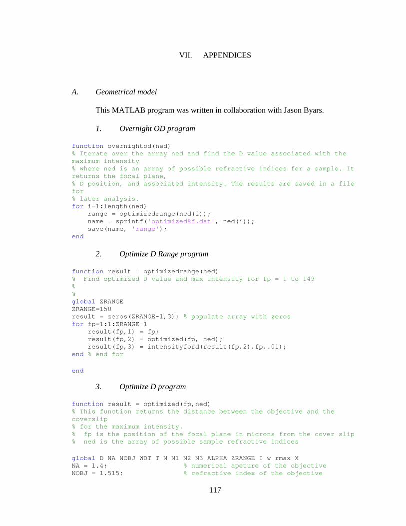
117
VII. APPENDICES
A. Geometrical model
This MATLAB program was written in collaboration with Jason Byars. 1. Overnight OD program function overnightod(ned) % Iterate over the array ned and find the D value associated with the maximum intensity % where ned is an array of possible refractive indices for a sample. It returns the focal plane, % D position, and associated intensity. The results are saved in a file for % later analysis. for i=1:length(ned) range = optimizedrange(ned(i)); name = sprintf('optimized%f.dat', ned(i)); save(name, 'range'); end 2. Optimize D Range program function result = optimizedrange(ned) % Find optimized D value and max intensity for fp = 1 to 149 % % global ZRANGE ZRANGE=150 result = zeros(ZRANGE-1,3); % populate array with zeros for fp=1:1:ZRANGE-1 result(fp,1) = fp; result(fp,2) = optimized(fp, ned); result(fp,3) = intensityford(result(fp,2),fp,.01); end % end for end 3. Optimize D program function result = optimized(fp,ned) % This function returns the distance between the objective and the coverslip % for the maximum intensity. % fp is the position of the focal plane in microns from the cover slip % ned is the array of possible sample refractive indices global D NA NOBJ WDT T N N1 N2 N3 ALPHA ZRANGE I w rmax X NA = 1.4; % numerical apeture of the objective NOBJ = 1.515; % refractive index of the objective

118
WOBJ = 150; % working distance of the objective in um T = 170; % cover slip thickness in microns WDT = WOBJ + T; % working distance + ideal coverslip thickness in um N = 1.51633; % actual refractive index of objective lens glass N1 = 1.515; % refractive index of the immersion fluid N2 = 1.515; % actual refractive index of cover glass N3 = ned; % hypothetical refractive index of the sample ALPHA = asin (NA/NOBJ); % apeture angle rmax = (WDT)*tan (ALPHA); % radius of the objective lens %step = 0.5; w = 4200; % radius of the back apeture in microns and pulse width % assume filled objective P = 2000; % power in uW I = 2*P/(3.14159*w^2); % initial intensity delta = 10^-58; % fluorophore cross section in m^4sec f = 82*10^6; % repetition rate of laser in Hz tau = 100*10-15; % temporal pulse width of laser in seconds lambda = 800*10^-9; % wavelength in meters X=0.1; % lateral range to include at fp %excitprob = delta*(P*10^-6)^2/(f^2*tau)*(NA^2/(2*1.0546*10^-34*3*10^8*lambda))^2; % rintensity is in microwatts! so plug it in here? %zrange 5-150 step 5 where zrange always <= WOBJ ZRANGE = 150; % distance from coverslip into the sample in um dmax = WOBJ-fp; % maximum depth into the sample in microns d= dmax; dstep = -1; maxintensity = 0.0; % integrated intensity disp(sprintf('doing fp %d', fp)); % loop over D range rough pass assuming after reaching a peak we can stop % searching for d = dmax:dstep:1 intensity = intensityford(d,fp,1); if maxintensity > intensity break; else maxintensity = intensity; end end % end d loop dmax = d+2; % search d-2 to d+2 for actual peak intensity location and value disp(sprintf('optimal d between %f and %f for dstep of %f intensity %f',dmax-2, dmax, dstep, maxintensity));

119
dstep = dstep / 10; % reduce step size on each pass to refine search % search cutoff of .0001 step size from emprical results while ( abs(dstep) >= .0001 ) maxintensity = 0; %disp(sprintf('%f:%f:%f',dmax,dstep,(dmax-20*abs(dstep)) )); for d = dmax:dstep:(dmax-20*abs(dstep)) intensity = intensityford(d,fp,1); if maxintensity > intensity break; else maxintensity = intensity; end end % end d loop d = d+1; dmax = d + 2*abs(dstep); %disp(sprintf('optimal d between %f and %f for dstep of %f intensity %f',dmax+2*dstep,dmax, dstep, maxintensity)); dstep = dstep / 10; end result = d + 10*abs(dstep); % move back to the d value that was the peak end %end function 4. Intensity program function intensity = intensityford(d,fp,rstep) % For a given distance between coverslip and objective, focal plane, and % step to integrate over the objective radius, return the intensity global rmax w arr = floor(rmax); % integrating over integer steps for practical time constraints intensity = 0; start = 1; R1 = 1; %search for doughnuts while (R1 < arr && R1 ~= 0) S1 = 0; % the S value (radius at the back apeture) associated with R1 S2 = 0; % the S value (radius at the back apeture) associated with R2 R1 = 0; % the first r position that contributes to the intensity R2 = 0; % the last r position that contributes to the intensity % find R1 for r = start:rstep:arr [beta,theta3, z, lower, upper] = thetans(r,d,fp); %disp(sprintf('fp %d d %d r %d %f <= %f <= %f',fp,d,r,lower, tan(theta3), upper)); if z < 0 continue; end % if within bounds the intensity contributes if (lower <= tan(theta3) && tan(theta3) <= upper) || ( fp-.1 <= z && z <= fp+.1 )

120
R1 = r; if R1 == 1 S1 = 0; else S1 = S(R1, beta); end break; end end %end for if (R1 == 0 || R1 == arr) %check for out of bound %disp(sprintf('fp %d d %d No R1', fp, d)); break; end % find R2 for r = R1+rstep:rstep:arr [beta,theta3, z, lower, upper] = thetans(r,d,fp); if z < 0 continue; end % if within bounds the intensity contributes if ((lower > tan(theta3) || tan(theta3) > upper) && ( fp-.1 > z || z > fp+.1 ) ) R2 = r-rstep; [beta,theta3, z, lower, upper] = thetans(R2,d,fp); S2 = S(R2, beta); break; end if (r == arr) R2 = rmax; S2 = S(R2, beta); end end %end for if (R2 == 0) %disp(sprintf('fp %d d %d R1 %d No R2',fp, d, R1)); break; end start = R2+rstep; % continue searching for contributing R values after R2 intensity = intensity + pi*w^2/2*abs(sintensity(S2)-sintensity(S1)); end %end while end function [beta,theta3,z,lower,upper] =thetans(r,d,fp) % This is a convenience function to perform calculations that occur in % several places. global WDT NOBJ N N1 N2 N3 T X alphar = atan (r/(WDT)); % assuming no refraction, the angle of light from radius beta = asin((NOBJ/N)*sin(alphar)); % the actual angle of light incident on the objective lens theta1 = asin (N/N1*sin (beta)); % refraction angles for the objective lens-immersion fluid interface theta2 = asin (N/N2*sin (beta)); % refraction angles for the immersion fluid-coverslip interface

121
theta3 = asin (N/N3*sin (beta)); % refraction angles for the coverslip-sample interface z = (r-d*tan(theta1)-T*tan(theta2))/tan(theta3); % depth into the sample where light from a cone with radius r will focus lower = (r-d*tan(theta1)-T*tan(theta2)-X)/fp; % lateral range around fp upper = (r-d*tan(theta1)-T*tan(theta2)+X)/fp; % lateral range around fp end function sposition = S(r, beta) % radial distance at the back apeture associated with r for a given beta global w NA N rmax sposition = (w-rmax)/(tan(asin(NA/N)))*tan(beta)+r; %disp(sprintf('(%f-%f)/(tan(asin(%f/%f))*tan(%f)+%f',w,rmax,NA,N,beta,r)); end function sint = sintensity(s) % intensity calculation for a given S position global I w sint = I*exp(-2*(s)^2/(w^2)); %disp(sprintf('r %.10f rmax %.10f beta %.10f S %.10f rintensity %.10f', r, rmax, beta,S(r,rmax,beta), arr)); end % warn about out of bounds later function zoff = zindex(z, r) % not used in final version global ZRANGE zoff = round(z); if (zoff <= 0 || zoff == NaN || zoff > ZRANGE) disp(sprintf('z is bad %f for r %f', z, r)); zoff = -1; end end function s = finds(r, start) % not used in final version global N NA w WDT NOBJ ALPHA alphar = atan (r/(WDT)); beta = asin((NOBJ/N)*sin(alphar)); rmax = (WDT)*tan (ALPHA); s = ((w-rmax)/(tan(asin(NA/N)))*tan(beta) + r) - start; s = abs(s); end function arr = findr(s) % not used in final version global WDT ALPHA rmax = (WDT)*tan (ALPHA); [arr, val] = fminbnd(@(x)finds(x, s), 0, rmax); %disp(sprintf('S %f R %f val %f', s, arr, val)); end

122
B. ImageJ plugins
1. Getting_Loaded_Olympus.java
import ij.*; import ij.io.*; import ij.plugin.*; import ij.process.*; import java.io.*; import java.util.Arrays; import java.util.Comparator; /** This filter just matches oif files. There is nothing exciting here. */ class OIFFilter implements FilenameFilter { public boolean accept(File dir, String name) { File foo = new File(dir.getPath() + File.separator + name); if (!foo.isFile()) return false; if (!foo.canRead()) return false; return (name.toLowerCase().endsWith(".oif")); } } /** This filter just matches tif files. There is nothing exciting here. */ class TiffFilter implements FilenameFilter { public boolean accept(File dir, String name) { File foo = new File(dir.getPath() + File.separator + name); if (!foo.isFile()) return false; if (!foo.canRead()) return false; return (name.toLowerCase().endsWith(".tif")); } } /** This comparator is used to determine the appropriate order of tiff files * based on channel and slice. */ class TIFFComparator implements Comparator<String> { public int compare(final String o1, final String o2) { int index = o1.lastIndexOf("_C0"); index = o1.indexOf("Z", index)+1; int end = index; while (Character.isDigit(o1.charAt(end))) end++;

123
int z1 = Integer.valueOf(o1.substring(index,end)).intValue(); index = o2.lastIndexOf("_C0"); index = o2.indexOf("Z", index)+1; end = index; while (Character.isDigit(o2.charAt(end))) end++; int z2 = Integer.valueOf(o2.substring(index,end)).intValue(); return z1-z2; } } /** This plugin quickly loads Olympus OIF files into ImageJ correctly dealing with stack with * greather than 1000 slices. * @author Jason Byars <[email protected]> * @version 0.001 */ public class Getting_Loaded_Olympus implements PlugIn { String[][] slices; String src; int channels; /** This is the main method of the plugin. It prompts the user for the path to the directory of tiffs * when not provided one as an argument. * @see ij.plugin.PlugIn#run(java.lang.String) * @param arg used to provide a single paramter, src when run from macros * */ public void run(String arg) { channels = 0; slices = null; src = null; if (IJ.versionLessThan("1.40")) { IJ.showMessage("ImageJ 1.40 or greater required."); return; } try { if (Macro.getOptions() == null) { if (!showDialog()) return; } else { src = Macro.getValue(Macro.getOptions(), "src", ""); if (src.trim() == "") { IJ.showStatus("Error: no folder specified");

124
return; } } if (!divineList()) return; load(); } catch (Exception e) { CharArrayWriter caw = new CharArrayWriter(); PrintWriter pw = new PrintWriter(caw); e.printStackTrace(pw); IJ.write(caw.toString()); IJ.showStatus(""); } IJ.register(Getting_Loaded_Olympus.class); } /** Get a list of all the tiffs in the folder. Sort the list appropriately by channel and * z section. * */ private boolean divineList() { try { File folder = new File(src); FilenameFilter filter = new TiffFilter(); String[] tlist = folder.list(filter); if (tlist == null) { IJ.showStatus("Error: could not find any tiffs"); return false; } if (tlist.length == 0) return false; StringBuffer pattern = new StringBuffer(); for(int i=0; tlist != null && i < tlist.length; i++) { int index = tlist[i].lastIndexOf("_C0"); String tmp = tlist[i].substring(index, index+5); if (pattern.indexOf(tmp) == -1) { pattern.append(tmp); channels++; } } //sort into channels in case there is an act of stupidity slices = new String[channels][]; int index=0; String chtmp = "";

125
for (int c=0; c<channels; c++) { slices[c] = new String[tlist.length/channels]; int count=0; //get the pattern for(int i=0; tlist != null && i < tlist.length; i++) { if (tlist[i] == null) continue; index = tlist[i].lastIndexOf("_C0"); String tmp = tlist[i].substring(index, index+5); if (chtmp.indexOf(tmp) == -1) { chtmp = tmp; break; } } for(int i=0; tlist != null && i < tlist.length; i++) { if (tlist[i] == null) continue; if (tlist[i].indexOf(chtmp) != -1) { slices[c][count++] = tlist[i]; tlist[i] = null; } } //sort along z for dumb numbering Arrays.sort(slices[c], new TIFFComparator()); } } catch (Exception e) { CharArrayWriter caw = new CharArrayWriter(); PrintWriter pw = new PrintWriter(caw); e.printStackTrace(pw); IJ.write(caw.toString()); IJ.showStatus(""); } return true; }
/** This method iterates over the list of tiffs and build large single channels stacks. * */ public void load() { Opener opener = new Opener(); opener.setSilentMode(true); ImagePlus imp = null; ImageStack stack = null; for(int c=0; c<channels; c++) { imp = opener.openImage(src, slices[c][0]);

126
stack = imp.getStack(); for (int i=1; i<slices[c].length; i++) { imp = opener.openImage(src, slices[c][i]); ImageProcessor ip = imp.getProcessor(); File nfo = new File(slices[c][i]); stack.addSlice(nfo.getName(), ip); imp = null; IJ.showStatus((i+1)+"/"+slices[c].length); IJ.showProgress(i+1, slices[c].length); } int end = slices[0][0].lastIndexOf("_C0"); String title = slices[0][0].substring(0,end); ImagePlus imp2 = new ImagePlus(title, stack); imp2.show(); } } /** Prompt the user for the location of the folder of tiffs. * */ public boolean showDialog() { DirectoryChooser dc = new DirectoryChooser("Select the folder of tiffs"); src = dc.getDirectory(); if (src == null) return false; return true; } void showAbout() { String title = "About " + getClass().getName() + "..."; IJ.showMessage(title, "This plugin open Olympus stacks with over 1000 slices correctly"); } void error() { String title = "About " + getClass().getName() + "..."; IJ.showMessage(title, "This plugin requires an Olympus folder of tiffs"); } }

127
2. Pam_Background.java
import ij.*; import ij.measure.*; import ij.plugin.*; /** Find the mean of the last 10 slices of a stack. * @author Jason Byars <[email protected]> * @version 0.001 */ public class Pam_Background implements PlugIn { ImagePlus imp; ResultsTable rt; //********************************************************************************* public Pam_Background() { makeResultTable(); IJ.register(Pam_Bead_Stats.class); } //********************************************************************************* /** Find the mean of the last 10 slices of a stack. */ private double last10Mean() { int orig = imp.getSlice(); int first = imp.getNSlices()-9; //-9 does 10 slices first = (first < 1) ? 1 : first; long total = 0; for (int i=first; i<=imp.getNSlices(); i++) { imp.setSlice(i); for (int y=0; y<imp.getHeight(); y++) { for (int x=0; x<imp.getWidth(); x++) { total += imp.getPixel(x,y)[0]; } } } imp.setSlice(orig); double mean = total / (10.0*imp.getWidth()*imp.getHeight()); return mean; }

128
//********************************************************************************* /** Create a results table. */ private void makeResultTable() { rt = new ResultsTable(); rt.reset(); rt.getFreeColumn("Mean"); //fields for array of data points } //********************************************************************************* /** Find the mean of the last 10 slices of a stack and show the results in the results table. * @see ij.plugin.PlugIn#run(java.lang.String) * @param arg used to provide a single paramter, src when run from macros */ public void run(String arg) { if (IJ.versionLessThan("1.40")) { IJ.showMessage("ImageJ 1.40 or greater required."); return; } imp = WindowManager.getCurrentImage(); if (imp==null) { IJ.showMessage("You must have images open for this plugin!"); return; } if (imp.getNSlices() < 10) { IJ.error("The stack has less than 10 slices. Try again hoser."); return; } double mean = last10Mean(); rt.incrementCounter(); rt.addLabel("Stack", imp.getTitle()); rt.addValue(0, mean); rt.show("Mean of last 10 slices"); } //********************************************************************************* void showAbout() {
129
String title = "About " + getClass().getName() + "..."; IJ.showMessage(title, "This plugin finds the mean for the last 10 slices in a stack."); } //********************************************************************************* void error() { IJ.showMessage(getClass().getName(), "Something went wrong."); } }
3. Pam_Bead_Stats.java
import ij.*; import ij.plugin.frame.*; import ij.measure.*; import ij.gui.*; import java.awt.*; import java.awt.event.*; /** Given a region of interest it, it finds the brighest point and averages with the specified * number of surrounding points. * @author Jason Byars <[email protected]> * @version 0.005 */ public class Pam_Bead_Stats extends PlugInFrame implements ActionListener { private static final long serialVersionUID = -8626748743748121467L; Panel panel; static Frame instance; GridBagConstraints gbc = new GridBagConstraints(); ImagePlus imp; Roi currentRoi; ResultsTable rt; TextField txtPlanes; TextField txtRadius; int planes; int radius; public Pam_Bead_Stats() { super("Pam_Bead_Stats v0.005"); if (IJ.versionLessThan("1.40")) {

130
IJ.showMessage("ImageJ 1.40 or greater required."); return; } if (instance!=null) { instance.toFront(); return; } instance = this; addKeyListener(IJ.getInstance()); makeResultTable(); showDialog(); IJ.register(Pam_Bead_Stats.class); } public void actionPerformed(ActionEvent e) { imp = WindowManager.getCurrentImage(); currentRoi = imp.getRoi(); if (imp==null) { IJ.beep(); IJ.showStatus("No image"); return; } if (currentRoi == null) { IJ.beep(); IJ.showStatus("No ROI"); return; } if (currentRoi.getType() == Roi.LINE) { IJ.beep(); IJ.showStatus("Rectangles or Ovals only!"); return; } String label = e.getActionCommand(); if (label==null) { IJ.showStatus("I have no idea what to do"); return; } try { planes = Integer.parseInt(txtPlanes.getText()); radius = Integer.parseInt(txtRadius.getText()); } catch (NumberFormatException n) { IJ.showMessage("Give me real numbers!"); return; }

131
if (planes < 1) { IJ.showMessage("Invalid number of planes. Try again hoser."); return; } if (radius < 1) { IJ.showMessage("Invalid radius. Try again hoser."); return; } if (label == "Measure") measureit(); else if (label == "Measure All") measureAll(); else if (label == "Dump ROI") dumpROI(); else imp.killRoi(); } private void dumpROI() { int[] value = {0,0,0,0}; int orig = imp.getSlice(); Rectangle bounds = currentRoi.getBounds(); ResultsTable tmp = new ResultsTable(); tmp.reset(); for (int x = (int) bounds.getX(); x <= (int) (bounds.getX() + bounds.getWidth()); x++) tmp.getFreeColumn("X"+x); int zmin = imp.getSlice() - planes; int zmax = imp.getSlice() + planes; if (zmin < 1) zmin = 1; if (zmax > imp.getNSlices()) zmax = imp.getNSlices(); for (int z = zmin; z <= zmax; z++) { imp.setSlice(z); for (int y = (int) bounds.getY(); y <= (int) (bounds.getY() + bounds.getHeight()); y++) { tmp.incrementCounter(); for (int x = (int) bounds.getX(); x <= (int) (bounds.getX() + bounds.getWidth()); x++) { if (currentRoi.contains(x,y)) value = imp.getPixel(x,y); else
132
value[0] = 0; tmp.addValue((int) (x-bounds.getX()), value[0]); } } } tmp.show("ROI x"+(int) bounds.getX()+" y"+ (int) bounds.getY()+" z"+imp.getSlice()); imp.setSlice(orig); } private int[] findPeak() { int zmin = imp.getSlice() - planes; int zmax = imp.getSlice() + planes; if (zmin < 1) zmin = 1; if (zmax > imp.getNSlices()) zmax = imp.getNSlices(); int[] peak = {0,0,0,0,0}; int[] value = {0,0,0,0}; int multi = 1; Rectangle bounds = currentRoi.getBounds(); for (int z = zmin; z <= zmax; z++) { imp.setSlice(z); for (int y = (int) bounds.getY(); y <= (int) (bounds.getY() + bounds.getHeight()); y++) { for (int x = (int) bounds.getX(); x <= (int) (bounds.getX() + bounds.getWidth()); x++) { if (!currentRoi.contains(x,y)) continue; value = imp.getPixel(x,y); if ( value[0] > peak[0] ) { peak[0] = value[0]; peak[1] = x; peak[2] = y; peak[3] = z; multi = 1; } else if (value[0] == peak[0]) { multi++; } } } } peak[4] = multi; return peak; }

133
private void measureAll() { RoiManager mgr = RoiManager.getInstance(); if (mgr == null) { IJ.beep(); IJ.showStatus("Roi Manager not open"); return; } Roi[] rois = mgr.getRoisAsArray(); int orig = imp.getSlice(); for (int i=0; i < rois.length; i++) { currentRoi = rois[i]; imp.setSlice(mgr.getSliceNumber(currentRoi.getName())); if (mgr.getSliceNumber(currentRoi.getName()) < 1) { IJ.error("I don't know what the slice is for ROI "+currentRoi.getName()); } measureit(); } imp.setSlice(orig); } private void measureit() { int orig = imp.getSlice(); int[] peak = findPeak(); int[] value = {0,0,0,0}; //ok do stats double intensity = 0; int voxels = 0; int xmin = peak[1]-radius; int xmax = peak[1]+radius; int ymin = peak[2]-radius; int ymax = peak[2]+radius; int zmin = peak[3]-radius; int zmax = peak[3]+radius; if ( xmin < 0 ) xmin = 0; if ( ymin < 0 ) ymin = 0; if ( zmin < 0 ) zmin = 0; if ( xmax > imp.getWidth()-1 ) xmax = imp.getWidth() - 1; if ( ymax > imp.getHeight()-1 ) ymax = imp.getHeight() - 1; if ( zmax > imp.getNSlices()-1 ) zmax = imp.getNSlices() - 1; for (int z = zmin; z <= zmax; z++) { imp.setSlice(z);

134
for (int y = ymin; y <= ymax; y++) { for (int x = xmin; x <= xmax; x++,voxels++) { value = imp.getPixel(x,y); intensity += value[0]; } } } imp.setSlice(orig); if (rt.getCounter()==0) makeResultTable(); //results table closed rt.incrementCounter(); rt.addLabel("Name",currentRoi.getName()); rt.addValue(0,peak[1]); rt.addValue(1,peak[2]); rt.addValue(2,peak[3]); rt.addValue(3,peak[0]); rt.addValue(4,intensity); rt.addValue(5,intensity/voxels); rt.addValue(6,peak[4]); rt.show("Results for Peak Pixel"); String s = "Peak "+peak[0]+" x: "+peak[1]+" y: "+peak[2]+" z: "+peak[3]; IJ.showStatus(s); } private void makeResultTable() { rt = new ResultsTable(); rt.reset(); rt.getFreeColumn("X"); rt.getFreeColumn("Y"); rt.getFreeColumn("Z"); rt.getFreeColumn("Peak"); rt.getFreeColumn("Total Intensity"); rt.getFreeColumn("Mean"); rt.getFreeColumn("Multiple"); } public void processWindowEvent(WindowEvent e) { super.processWindowEvent(e); if (e.getID()==WindowEvent.WINDOW_CLOSING) { instance = null; } } private void set_gbc(int row, int column, int width, int height, int fill) { set_gbc(row,column,width,height,fill,0,0);

135
} private void set_gbc(int row, int column, int width, int height, int fill, int padx, int pady) { gbc.gridy = row; gbc.gridx = column; gbc.gridwidth = width; gbc.gridheight = height; gbc.fill = fill; // GridBagConstraints.NONE .HORIZONTAL .VERTICAL .BOTH gbc.ipadx = padx; gbc.ipady = pady; // leave other fields (eg, anchor) unchanged. } public void showDialog() { //because windows is stupid setLayout(new FlowLayout()); panel = new Panel(); GridBagLayout gridbag = new GridBagLayout(); panel.setLayout(gridbag); String s = "Select a region around a bead."; Label l = new Label(s); set_gbc(0,0,4,1, GridBagConstraints.HORIZONTAL, 0, 0); gridbag.setConstraints(l,gbc); panel.add(l, gbc); s = "Specify how far above and below to look."; l = new Label(s); set_gbc(1,0,4,1, GridBagConstraints.HORIZONTAL, 0, 0); gridbag.setConstraints(l,gbc); panel.add(l, gbc); s = "Specify the radius to average."; l = new Label(s); set_gbc(2,0,4,1, GridBagConstraints.HORIZONTAL, 0, 10); gridbag.setConstraints(l,gbc); panel.add(l, gbc); l = new Label("Planes to check", Label.RIGHT); set_gbc(3,0,2,1, GridBagConstraints.HORIZONTAL); gridbag.setConstraints(l,gbc); panel.add(l, gbc); txtPlanes = new TextField("10", 20); set_gbc(3,2,2,1, GridBagConstraints.NONE); gridbag.setConstraints(txtPlanes,gbc); panel.add(txtPlanes, gbc); l = new Label("Radius", Label.RIGHT); set_gbc(4,0,2,1, GridBagConstraints.HORIZONTAL);

136
gridbag.setConstraints(l,gbc); panel.add(l, gbc); txtRadius = new TextField("1", 20); set_gbc(4,2,2,1, GridBagConstraints.NONE); gridbag.setConstraints(txtRadius,gbc); panel.add(txtRadius, gbc); Button b = new Button("Measure"); b.addActionListener(this); b.addKeyListener(IJ.getInstance()); set_gbc(5,0,1,1, GridBagConstraints.NONE); gridbag.setConstraints(b,gbc); panel.add(b); b = new Button("Measure All"); b.addActionListener(this); b.addKeyListener(IJ.getInstance()); set_gbc(5,1,1,1, GridBagConstraints.NONE); gridbag.setConstraints(b,gbc); panel.add(b); b = new Button("Dump ROI"); b.addActionListener(this); b.addKeyListener(IJ.getInstance()); set_gbc(5,2,1,1, GridBagConstraints.NONE); gridbag.setConstraints(b,gbc); panel.add(b); b = new Button("Clear ROI"); b.addActionListener(this); b.addKeyListener(IJ.getInstance()); set_gbc(5,3,1,1, GridBagConstraints.NONE); gridbag.setConstraints(b,gbc); panel.add(b); add(panel); pack(); GUI.center(this); setVisible(true); } void showAbout() { String title = "About " + getClass().getName() + "..."; IJ.showMessage(title, "This app takes a region, finds the brightest point and averages it with pixels in a radius of x."); } void error() {

137
IJ.showMessage("Pam_Bead_Stats", "This plugin requires a definied region to work"); } }
4. Pam_Bead_Stats2.java
import ij.*; import ij.plugin.frame.*; import ij.measure.*; import ij.gui.*; import java.awt.*; import java.awt.event.*; import java.io.*; /** Given a region of interest it, it finds the brighest point and averages with the specified * number of surrounding points. * @author Jason Byars <[email protected]> * @version 0.008 */ public class Pam_Bead_Stats2 extends PlugInFrame implements ActionListener { private static final long serialVersionUID = 3102557507830434785L; /** A convenient class to track all the stats generated from each bright point. * @author Jason Byars <[email protected]> */ class PamResults { public int hotPixel3x3; //hottest pixel in the selected integrated intensity region public int hotPixelRoi; //hottest pixel in the whole region public int multiple; //number of regions w/ public int x; public int y; public int z; public double mean; public double stdev; public double background; public double backgroundStdev; public double totalIntensity; public int voxels; String stackName; String roiName;

138
/** Appends the stats for this point to a given results table. * @param rt the results table to append the stats to */ void reportRT(ResultsTable rt) { rt.incrementCounter(); rt.addLabel("Name",roiName); rt.addValue(0, hotPixel3x3); // hottest pixel 3x3 rt.addValue(1, hotPixelRoi); // hottest pixel roi rt.addValue(2, multiple); // number of regions w/ same total intensity rt.addValue(3, x); // x rt.addValue(4, y); // y rt.addValue(5, z); // z rt.addValue(6, totalIntensity); // total intensity rt.addValue(7, mean); // mean rt.addValue(8, stdev); // standard deviation of the mean rt.addValue(9, background); // mean of last 10 planes in the stack rt.addValue(10, backgroundStdev); // standard deviation of the background mean } /** Appends the stats for this point to a given csv file. * @param bf the BufferedWriter for the desired csv file */ void reportCSV(BufferedWriter bf) { String s = String.format("%s,%s,%d,%d,%d,%d,%d,%d,%f,%f,%f,%f,%f", stackName, roiName, hotPixel3x3, hotPixelRoi, multiple, x,y,z, mean, stdev, background, backgroundStdev, mean-background); try { bf.write(s); bf.newLine(); } catch (IOException e) { System.err.println(e); }
139
} }; Panel panel; static Frame instance; GridBagConstraints gbc = new GridBagConstraints(); ImagePlus imp; Roi currentRoi; PamResults result; ResultsTable rt; TextField txtPlanes; TextField txtRadius; int planes; int radius; int peakIntensity; int voxels; double persistentbkg; double persistentbkgstdev; BufferedWriter csvout; //********************************************************************************* public Pam_Bead_Stats2() { super("Pam_Bead_Stats2 v0.008"); if (IJ.versionLessThan("1.40")) { IJ.showMessage("ImageJ 1.40 or greater required."); return; } if (instance!=null) { instance.toFront(); return; } instance = this; addKeyListener(IJ.getInstance()); IJ.register(Pam_Bead_Stats2.class); } //********************************************************************************* public void actionPerformed(ActionEvent e) { imp = WindowManager.getCurrentImage(); currentRoi = imp.getRoi();

140
if (imp==null) { IJ.beep(); IJ.showStatus("No image"); return; } if (currentRoi == null) { IJ.beep(); IJ.showStatus("No ROI"); return; } if (currentRoi.getType() == Roi.LINE) { IJ.beep(); IJ.showStatus("Rectangles or Ovals only!"); return; } String label = e.getActionCommand(); if (label==null) { IJ.showStatus("I have no idea what to do"); return; } try { planes = Integer.parseInt(txtPlanes.getText()); radius = Integer.parseInt(txtRadius.getText()); } catch (NumberFormatException n) { IJ.showMessage("Give me real numbers!"); return; } if (!validateArgs()) return; if (label == "Measure") measureit(); else if (label == "Measure All") measureAll(); else if (label == "Dump ROI") dumpROI(); else imp.killRoi(); } //********************************************************************************* private void dumpROI() { int[] value = {0,0,0,0}; int orig = imp.getSlice();

141
Rectangle bounds = currentRoi.getBounds(); ResultsTable tmp = new ResultsTable(); tmp.reset(); for (int x = (int) bounds.getX(); x <= (int) (bounds.getX() + bounds.getWidth()); x++) tmp.getFreeColumn("X"+x); int zmin = imp.getSlice() - planes; int zmax = imp.getSlice() + planes; if (zmin < 1) zmin = 1; if (zmax > imp.getNSlices()) zmax = imp.getNSlices(); for (int z = zmin; z <= zmax; z++) { imp.setSlice(z); for (int y = (int) bounds.getY(); y <= (int) (bounds.getY() + bounds.getHeight()); y++) { tmp.incrementCounter(); for (int x = (int) bounds.getX(); x <= (int) (bounds.getX() + bounds.getWidth()); x++) { if (currentRoi.contains(x,y)) value = imp.getPixel(x,y); else value[0] = 0; tmp.addValue((int) (x-bounds.getX()), value[0]); } } } tmp.show("ROI x"+(int) bounds.getX()+" y"+ (int) bounds.getY()+" z"+imp.getSlice()); imp.setSlice(orig); } //********************************************************************************* private void findPeak() { int zmin = imp.getSlice() - planes; int zmax = imp.getSlice() + planes; if (zmin < 1) zmin = 1; if (zmax > imp.getNSlices()) zmax = imp.getNSlices(); double value = 0; int multi = 1; Rectangle bounds = currentRoi.getBounds(); for (int z = zmin; z <= zmax; z++) { imp.setSlice(z);

142
for (int y = (int) bounds.getY(); y <= (int) bounds.getY() + (int) bounds.getHeight(); y++) { for (int x = (int) bounds.getX(); x <= (int) bounds.getX() + (int) bounds.getWidth(); x++) { if (!currentRoi.contains(x,y)) continue; value = integratedIntensity(x,y,z); if ( peakIntensity > result.hotPixelRoi ) result.hotPixelRoi = peakIntensity; if ( (int) value > result.totalIntensity ) { result.totalIntensity = (int) value; result.x = x; result.y = y; result.z = z; result.voxels = voxels; result.hotPixel3x3 = peakIntensity; multi = 1; } else if ((int) value == result.totalIntensity) { multi++; } } } } result.mean = result.totalIntensity/result.voxels; result.stdev = integratedStdev(result.x,result.y,result.z, result.mean); result.multiple = multi; return; } //********************************************************************************* private double integratedIntensity(int x, int y, int z) { double intensity = 0; voxels = 0; peakIntensity = 0; int[] value = {0,0,0,0}; int xmin = x-radius; int xmax = x+radius; int ymin = y-radius; int ymax = y+radius; int zmin = z-radius; int zmax = z+radius; if ( xmin < 0 ) xmin = 0; if ( ymin < 0 ) ymin = 0; if ( zmin < 1 ) zmin = 1; if ( xmax > imp.getWidth()-1 ) xmax = imp.getWidth() - 1;

143
if ( ymax > imp.getHeight()-1 ) ymax = imp.getHeight() - 1; if ( zmax > imp.getNSlices() ) zmax = imp.getNSlices(); for (z = zmin; z <= zmax; z++) { imp.setSlice(z); for (y = ymin; y <= ymax; y++) { for (x = xmin; x <= xmax; x++,voxels++) { value = imp.getPixel(x,y); intensity += value[0]; if (value[0] > peakIntensity) peakIntensity = value[0]; } } } return intensity; } //********************************************************************************* private double integratedStdev(int x, int y, int z, double mean) { double total = 0; double voxels = 0; int xmin = x-radius; int xmax = x+radius; int ymin = y-radius; int ymax = y+radius; int zmin = z-radius; int zmax = z+radius; if ( xmin < 0 ) xmin = 0; if ( ymin < 0 ) ymin = 0; if ( zmin < 1 ) zmin = 1; if ( xmax > imp.getWidth()-1 ) xmax = imp.getWidth() - 1; if ( ymax > imp.getHeight()-1 ) ymax = imp.getHeight() - 1; if ( zmax > imp.getNSlices() ) zmax = imp.getNSlices(); for (z = zmin; z <= zmax; z++) { imp.setSlice(z); for (y = ymin; y <= ymax; y++) { for (x = xmin; x <= xmax; x++,voxels++) { int value = imp.getPixel(x,y)[0]; total += Math.pow(value - mean, 2); } } } double stdev = Math.sqrt(total/(voxels-1)); return stdev; }

144
//********************************************************************************* private double last10Mean() { int orig = imp.getSlice(); int first = imp.getNSlices()-9; //-9 does 10 slices first = (first < 1) ? 1 : first; long total = 0; for (int i=first; i<=imp.getNSlices(); i++) { imp.setSlice(i); for (int y=0; y<imp.getHeight(); y++) { for (int x=0; x<imp.getWidth(); x++) { total += imp.getPixel(x,y)[0]; } } } imp.setSlice(orig); double mean = total / (10.0*imp.getWidth()*imp.getHeight()); return mean; } //********************************************************************************* private double last10Stdev(double mean) { int orig = imp.getSlice(); int first = imp.getNSlices()-9; //-9 does 10 slices first = (first < 1) ? 1 : first; double total = 0; for (int i=first; i<=imp.getNSlices(); i++) { imp.setSlice(i); for (int y=0; y<imp.getHeight(); y++) { for (int x=0; x<imp.getWidth(); x++) { total += Math.pow(imp.getPixel(x,y)[0] - mean, 2); } } } imp.setSlice(orig); double stdev = Math.sqrt(total/(imp.getWidth()*imp.getHeight()*(imp.getNSlices()-first+1)-1)); return stdev; } //********************************************************************************* private void measureAll() { RoiManager mgr = RoiManager.getInstance(); if (mgr == null) {

145
IJ.beep(); IJ.showStatus("Roi Manager not open"); return; } Roi[] rois = mgr.getRoisAsArray(); persistentbkg = last10Mean(); persistentbkgstdev = last10Stdev(persistentbkg); int orig = imp.getSlice(); for (int i=0; i < rois.length; i++) { currentRoi = rois[i]; imp.setSlice(mgr.getSliceNumber(currentRoi.getName())); if (mgr.getSliceNumber(currentRoi.getName()) < 1) { IJ.error("I don't know what the slice is for ROI "+currentRoi.getName()); } measureit(); } imp.setSlice(orig); persistentbkg = -1; persistentbkgstdev = -1; } //********************************************************************************* private void measureit() { int orig = imp.getSlice(); result = new PamResults(); result.stackName = imp.getTitle(); result.roiName = currentRoi.getName(); findPeak(); //int[] value = {0,0,0,0}; //peakIntensity = 0; //ok do stats imp.setSlice(orig); //these ops are constant for the stack, don't do them every time! if (persistentbkg >= 0 ) { result.background = persistentbkg; result.backgroundStdev = persistentbkgstdev; } else { result.background = last10Mean(); result.backgroundStdev = last10Stdev(result.background); }

146
if ( rt == null ) { // macro version! result.reportCSV(csvout); } else { if (rt.getCounter()==0) makeResultTable(); //results table closed result.reportRT(rt); rt.show("Results Integrated peak"); } String s = "Peak "+result.totalIntensity+" x: "+result.x+" y: "+result.y+" z: "+result.z; IJ.showStatus(s); result = null; } //********************************************************************************* private void makeResultTable() { rt = new ResultsTable(); rt.reset(); rt.getFreeColumn("Hottest Pixel 3x3"); rt.getFreeColumn("Hottest Pixel ROI"); rt.getFreeColumn("Multiple"); rt.getFreeColumn("X"); rt.getFreeColumn("Y"); rt.getFreeColumn("Z"); rt.getFreeColumn("Total Intensity"); rt.getFreeColumn("Mean"); rt.getFreeColumn("Stdev"); rt.getFreeColumn("Background"); rt.getFreeColumn("Background Stdev"); } //********************************************************************************* public void processWindowEvent(WindowEvent e) { super.processWindowEvent(e); if (e.getID()==WindowEvent.WINDOW_CLOSING) { instance = null; } } //********************************************************************************* public void run(String arg) { String options = ""; String csvname = "";

147
if (IJ.versionLessThan("1.40")) { IJ.showMessage("ImageJ 1.40 or greater required."); return; } persistentbkg = -1; persistentbkgstdev = -1; if (Macro.getOptions() == null) { makeResultTable(); showDialog(); } else { //validation options = Macro.getOptions(); imp = WindowManager.getCurrentImage(); if (imp == null) return; try { planes = Integer.parseInt(Macro.getValue(options, "planes", "10")); radius = Integer.parseInt(Macro.getValue(options, "radius", "1")); csvname = Macro.getValue(options, "csv", imp.getTitle()); } catch (NumberFormatException e) { IJ.error("At least one of the arguments is not parseable! " + options); } if (!validateArgs()) return; try { if (!csvname.toLowerCase().endsWith("csv")) csvname += ".csv"; File csv = new File(csvname); csvout = new BufferedWriter(new FileWriter(csv)); csvout.write("planes," + planes + ",radius," + radius); csvout.newLine(); csvout.write("image name,region name,hottest pixel 3x3,hottest pixel roi,multiple,x,y,z,mean,mean stdev,background,background stdev,mean-background"); csvout.newLine(); measureAll(); csvout.close(); } catch (IOException e) { System.err.println(e); } } }

148
//********************************************************************************* private void set_gbc(int row, int column, int width, int height, int fill) { set_gbc(row,column,width,height,fill,0,0); } //********************************************************************************* private void set_gbc(int row, int column, int width, int height, int fill, int padx, int pady) { gbc.gridy = row; gbc.gridx = column; gbc.gridwidth = width; gbc.gridheight = height; gbc.fill = fill; // GridBagConstraints.NONE .HORIZONTAL .VERTICAL .BOTH gbc.ipadx = padx; gbc.ipady = pady; // leave other fields (eg, anchor) unchanged. } //********************************************************************************* private boolean validateArgs() { if (planes < 1) { IJ.showMessage("Invalid number of planes. Try again hoser."); return false; } if (radius < 1) { IJ.showMessage("Invalid radius. Try again hoser."); return false; } return true; } //********************************************************************************* public void showDialog() { //because windows is stupid setLayout(new FlowLayout()); panel = new Panel(); GridBagLayout gridbag = new GridBagLayout(); panel.setLayout(gridbag); String s = "Select a region around a bead.";

149
Label l = new Label(s); set_gbc(0,0,4,1, GridBagConstraints.HORIZONTAL, 0, 0); gridbag.setConstraints(l,gbc); panel.add(l, gbc); s = "Specify how far above and below to look."; l = new Label(s); set_gbc(1,0,4,1, GridBagConstraints.HORIZONTAL, 0, 0); gridbag.setConstraints(l,gbc); panel.add(l, gbc); s = "Specify the radius to average."; l = new Label(s); set_gbc(2,0,4,1, GridBagConstraints.HORIZONTAL, 0, 10); gridbag.setConstraints(l,gbc); panel.add(l, gbc); l = new Label("Planes to check", Label.RIGHT); set_gbc(3,0,2,1, GridBagConstraints.HORIZONTAL); gridbag.setConstraints(l,gbc); panel.add(l, gbc); txtPlanes = new TextField("10", 20); set_gbc(3,2,2,1, GridBagConstraints.NONE); gridbag.setConstraints(txtPlanes,gbc); panel.add(txtPlanes, gbc); l = new Label("Radius", Label.RIGHT); set_gbc(4,0,2,1, GridBagConstraints.HORIZONTAL); gridbag.setConstraints(l,gbc); panel.add(l, gbc); txtRadius = new TextField("1", 20); set_gbc(4,2,2,1, GridBagConstraints.NONE); gridbag.setConstraints(txtRadius,gbc); panel.add(txtRadius, gbc); Button b = new Button("Measure"); b.addActionListener(this); b.addKeyListener(IJ.getInstance()); set_gbc(5,0,1,1, GridBagConstraints.NONE); gridbag.setConstraints(b,gbc); panel.add(b); b = new Button("Measure All"); b.addActionListener(this); b.addKeyListener(IJ.getInstance()); set_gbc(5,1,1,1, GridBagConstraints.NONE); gridbag.setConstraints(b,gbc); panel.add(b); b = new Button("Dump ROI"); b.addActionListener(this); b.addKeyListener(IJ.getInstance()); set_gbc(5,2,1,1, GridBagConstraints.NONE);

150
gridbag.setConstraints(b,gbc); panel.add(b); b = new Button("Clear ROI"); b.addActionListener(this); b.addKeyListener(IJ.getInstance()); set_gbc(5,3,1,1, GridBagConstraints.NONE); gridbag.setConstraints(b,gbc); panel.add(b); add(panel); pack(); GUI.center(this); setVisible(true); } //********************************************************************************* void showAbout() { String title = "About " + getClass().getName() + "..."; IJ.showMessage(title, "This app takes a region, finds the brightest point and averages it with pixels in a radius of x."); } //********************************************************************************* void error() { IJ.showMessage("Pam_Bead_Stats2", "This plugin requires a definied region to work"); } }
5. Pam_Bead_Stats3.java
import ij.*; import ij.plugin.frame.*; import ij.plugin.filter.*; import ij.measure.*; import ij.process.*; import ij.gui.*; import java.awt.*; import java.awt.event.*; /** Given a region of interest it, it finds the brighest subregion. It then takes the central pixel, return a range along * Z, finds the max of the range, and does the FWHM.

151
* @author Jason Byars <[email protected]> * @version 0.004 */ public class Pam_Bead_Stats3 extends PlugInFrame implements ActionListener { private static final long serialVersionUID = 421671022521828779L; Panel panel; static Frame instance; GridBagConstraints gbc = new GridBagConstraints(); ImagePlus imp; Roi currentRoi; ResultsTable rt; TextField txtPlanes; TextField txtGaussianRadius; TextField txtMaxRadius; TextField txtIntegratedIntensity; TextField txtRange; GaussianBlur blur; double gaussianRadius; int maxRadius; int planes; int radius; int range; int peakIntensity; int voxels; int[] zrange; static final int window = 21; //size of substack for filtering //********************************************************************************* public Pam_Bead_Stats3() { super("Pam_Bead_Stats3 v0.004"); if (IJ.versionLessThan("1.40")) { IJ.showMessage("ImageJ 1.40 or greater required."); return; } if (instance!=null) { instance.toFront(); return; } instance = this; addKeyListener(IJ.getInstance()); //makeResultTable(); showDialog();
152
IJ.register(Pam_Bead_Stats3.class); } //********************************************************************************* public void actionPerformed(ActionEvent e) { imp = WindowManager.getCurrentImage(); currentRoi = imp.getRoi(); if (imp==null) { IJ.beep(); IJ.showStatus("No image"); return; } if (currentRoi == null) { IJ.beep(); IJ.showStatus("No ROI"); return; } if (currentRoi.getType() == Roi.LINE) { IJ.beep(); IJ.showStatus("Rectangles or Ovals only!"); return; } String label = e.getActionCommand(); if (label==null) { IJ.showStatus("I have no idea what to do"); return; } try { planes = Integer.parseInt(txtPlanes.getText()); range = Integer.parseInt(txtRange.getText()); radius = Integer.parseInt(txtIntegratedIntensity.getText()); maxRadius = Integer.parseInt(txtMaxRadius.getText()); gaussianRadius = Double.parseDouble(txtGaussianRadius.getText()); } catch (NumberFormatException n) { IJ.showMessage("Give me real numbers!"); return; } if (planes < 1) { IJ.showMessage("Invalid number of planes. Try again hoser."); return; } if (radius < 1) { IJ.showMessage("Invalid radius. Try again hoser."); return;

153
} //We're actually going to do something if (label == "Measure") { makeResultTable(); measureit(); } else if (label == "Measure All") { makeResultTable(); measureAll(); } else if (label == "Dump ROI") dumpROI(); else imp.killRoi(); } //********************************************************************************* void displayFWHM(int[] peak, int[] subpeak, double[] fwhm, double[] gfwhm, ImagePlus tmp, ImagePlus gtmp, int zmin, int zmax, int zpad) { double [] x = new double[tmp.getNSlices()]; double [] y = new double[tmp.getNSlices()]; double [] result = new double[tmp.getNSlices()]; for (int z=1; z<=tmp.getNSlices(); z++) { x[z-1] = z+zmin-1; tmp.setSlice(z); y[z-1] = tmp.getPixel(subpeak[0],subpeak[1])[0]; } if (gaussianRadius > 0) { for (int z=1; z<=gtmp.getNSlices(); z++) { gtmp.setSlice(z); result[z-1] = gtmp.getPixel(subpeak[0],subpeak[1])[0]; } } Plot p = new Plot("FWHM for "+currentRoi.getName(),"Z plane","Intensity", (double[]) null,(double[]) null); p.setLimits(zmin, zmax, 0, fwhm[4]+100); p.setColor(Color.blue); p.addPoints(x,y,PlotWindow.CIRCLE); p.setColor(Color.red); if (gaussianRadius > 0) { p.setColor(Color.green); p.addPoints(x,result, PlotWindow.X); // add a fwhm curve double[] x2 = {gfwhm[1]+zpad,gfwhm[2]+zpad};

154
double[] y2 = {gfwhm[4]/2.0, gfwhm[4]/2.0}; double[] x3 = {gfwhm[3]+zpad, gfwhm[3]+zpad}; double[] y3 = {gfwhm[4]/2.0, gfwhm[4]}; p.setColor(Color.red); p.addPoints(x2,y2,PlotWindow.X); p.addPoints(x2,y2,PlotWindow.LINE); p.addPoints(x3,y3,PlotWindow.LINE); } else { double[] x2 = {gfwhm[1]+zpad,gfwhm[2]+zpad}; double[] y2 = {gfwhm[4]/2.0, gfwhm[4]/2.0}; double[] x3 = {gfwhm[3]+zpad, gfwhm[3]+zpad}; double[] y3 = {gfwhm[4]/2.0, gfwhm[4]}; p.setColor(Color.red); p.addPoints(x2,y2,PlotWindow.X); p.addPoints(x2,y2,PlotWindow.LINE); p.addPoints(x3,y3,PlotWindow.LINE); } // add label p.setColor(Color.black); //p.changeFont(new Font("Helvetica", Font.PLAIN, 24)); p.addLabel(0.02, 0.1, String.format("Center: %d,%d,%d",peak[0],peak[1],peak[2])); p.addLabel(0.02, 0.2, "Max pixel: "+fwhm[4]); if (fwhm[0] > 0) p.addLabel(0.02, 0.3, String.format("FWHM: %.2f",fwhm[0])); else p.addLabel(0.02, 0.3, String.format("FWHM: failed",fwhm[0])); if (gaussianRadius > 0) { p.addLabel(0.02, 0.4, "Gauss Max pixel: "+gfwhm[4]); if (gfwhm[0] > 0) p.addLabel(0.02, 0.5, String.format("Gauss FWHM: %.2f",gfwhm[0])); else p.addLabel(0.02, 0.5, String.format("Gauss FWHM: failed",gfwhm[0])); } //p.changeFont(new Font("Helvetica", Font.PLAIN, 16)); p.setColor(Color.lightGray); p.show(); }

155
//********************************************************************************* private void dumpROI() { int[] value = {0,0,0,0}; int orig = imp.getSlice(); Rectangle bounds = currentRoi.getBounds(); ResultsTable tmp = new ResultsTable(); tmp.reset(); for (int x = (int) bounds.getX(); x <= (int) (bounds.getX() + bounds.getWidth()); x++) tmp.getFreeColumn("X"+x); int zmin = imp.getSlice() - planes; int zmax = imp.getSlice() + planes; if (zmin < 1) zmin = 1; if (zmax > imp.getNSlices()) zmax = imp.getNSlices(); for (int z = zmin; z <= zmax; z++) { imp.setSlice(z); for (int y = (int) bounds.getY(); y <= (int) (bounds.getY() + bounds.getHeight()); y++) { tmp.incrementCounter(); for (int x = (int) bounds.getX(); x <= (int) (bounds.getX() + bounds.getWidth()); x++) { if (currentRoi.contains(x,y)) value = imp.getPixel(x,y); else value[0] = 0; tmp.addValue((int) (x-bounds.getX()), value[0]); } } } tmp.show("ROI x"+(int) bounds.getX()+" y"+ (int) bounds.getY()+" z"+imp.getSlice()); imp.setSlice(orig); } //********************************************************************************* private double[] findFWHM(int[] peak, ImagePlus tmp) { double [] fwhm = {-1, 0,0,0,0}; final int x = peak[0]; final int y = peak[1]; int z = peak[2]; //int zmin = peak[2]-range;
156
//if ( zmin < 1 ) zmin = 1; //int zmax = peak[2]+range; //if ( zmax > tmp.getNSlices() ) zmax = tmp.getNSlices(); //find peak pixel, start w/ center and work out tmp.setSlice(z); double limit = tmp.getPixel(x,y)[0]; for(int zed = peak[2]-maxRadius; zed<= peak[2]+maxRadius; zed++) { tmp.setSlice(zed); int value = tmp.getPixel(x,y)[0]; if (value > limit) { z = zed; limit = value; } } IJ.write(String.format("value %f z %d", limit, z)); fwhm[3] = z; fwhm[4] = limit; limit/=2.0; int i=0; double x1=0, x2=0, left=0, right=0, slope=0, offset=0; for (i=z; i>=1; i--) { tmp.setSlice(i); if (tmp.getPixel(x,y)[0] <= limit) { //interpolate x1 = tmp.getPixel(x,y)[0]; tmp.setSlice(i+1); x2 = tmp.getPixel(x,y)[0]; offset = limit - x1; slope = x2 - x1; left = i + (offset/slope); break; } } if (i<1) return fwhm; //out of bounds for (i=z; i<=tmp.getNSlices(); i++) { tmp.setSlice(i); if (tmp.getPixel(x,y)[0] <= limit) { //interpolate x2 = tmp.getPixel(x,y)[0]; tmp.setSlice(i-1); x1 = tmp.getPixel(x,y)[0]; offset = limit - x1; slope = x2 - x1;
157
right = i-1 + (offset/slope); break; } } if (i>tmp.getNSlices()) return fwhm; //out of bounds fwhm[0] = right - left; fwhm[1] = left; fwhm[2] = right; return fwhm; } //********************************************************************************* private int[] findPeak() { int zmin = imp.getSlice() - planes; int zmax = imp.getSlice() + planes; if (zmin < 1) zmin = 1; if (zmax > imp.getNSlices()) zmax = imp.getNSlices(); int[] peak = {0,0,0,0}; int value = 0; Rectangle bounds = currentRoi.getBounds(); for (int z = zmin; z <= zmax; z++) { imp.setSlice(z); for (int y = (int) bounds.getY(); y <= (int) bounds.getY() + (int) bounds.getHeight(); y++) { for (int x = (int) bounds.getX(); x <= (int) bounds.getX() + (int) bounds.getWidth(); x++) { if (!currentRoi.contains(x,y)) continue; value = (int) integratedIntensity(x,y,z); if ( value > peak[3] ) { peak[0] = x; peak[1] = y; peak[2] = z; peak[3] = value; } } } } return peak; } //********************************************************************************* private void GaussIt(ImagePlus tmp, double rad) {

158
ImageProcessor ip = tmp.getProcessor(); if (blur == null) blur = new GaussianBlur(); for (int i=1; i<tmp.getNSlices(); i++) { tmp.setSlice(i); blur.blur(ip,rad); } tmp.updateImage(); } //********************************************************************************* private double integratedIntensity(int x, int y, int z) { double intensity = 0; voxels = 0; int[] value = {0,0,0,0}; int xmin = x-radius; int xmax = x+radius; int ymin = y-radius; int ymax = y+radius; int zmin = z-radius; int zmax = z+radius; if ( xmin < 0 ) xmin = 0; if ( ymin < 0 ) ymin = 0; if ( zmin < 1 ) zmin = 1; if ( xmax > imp.getWidth()-1 ) xmax = imp.getWidth() - 1; if ( ymax > imp.getHeight()-1 ) ymax = imp.getHeight() - 1; if ( zmax > imp.getNSlices() ) zmax = imp.getNSlices(); for (z = zmin; z <= zmax; z++) { imp.setSlice(z); for (y = ymin; y <= ymax; y++) { for (x = xmin; x <= xmax; x++,voxels++) { value = imp.getPixel(x,y); intensity += value[0]; } } } return intensity; } //********************************************************************************* //odd dimensions only, no funny business private ImagePlus makeSubStack(String name, int x, int y, int zmin, int zmax, int length, int width ) {

159
final int xmin = x-(length/2); //final int xmax = x+(length/2); final int ymin = y-(width/2); //final int ymax = y+(width/2); /* int zmin = z-(depth/2); int zmax = z+(depth/2); if (zmin < 1) { depth-= ( 1-zmin); zmin = 1; } if (zmax > imp.getNSlices()) { depth-=(zmax-imp.getNSlices()); zmax = imp.getNSlices(); } */ ImagePlus tmp = NewImage.createShortImage(name, length, width,zmax-zmin+1, NewImage.FILL_BLACK); ImageProcessor ip = tmp.getProcessor(); int[] data = new int[length*4]; for (int i=zmin,w=1; i<=zmax; i++,w++) { imp.setSlice(i); tmp.setSlice(w); for (int j=0; j<width; j++) { imp.getProcessor().getRow(xmin, j + ymin, data, length); ip.putRow(0,j, data,length); } } tmp.updateImage(); return tmp; } //********************************************************************************* private void measureAll() { RoiManager mgr = RoiManager.getInstance(); if (mgr == null) { IJ.beep(); IJ.showStatus("Roi Manager not open"); return; } Roi[] rois = mgr.getRoisAsArray(); int orig = imp.getSlice();

160
for (int i=0; i < rois.length; i++) { currentRoi = rois[i]; imp.setSlice(mgr.getSliceNumber(currentRoi.getName())); if (mgr.getSliceNumber(currentRoi.getName()) < 1) { IJ.error("I don't know what the slice is for ROI "+currentRoi.getName()); } measureit(); } imp.setSlice(orig); } //********************************************************************************* private void measureit() { final int orig = imp.getSlice(); Duplicater d = new Duplicater(); ImagePlus tmp, gtmp; try { int[] peak = findPeak(); int[] subpeak = {10,10,range+1}; int zmin=peak[2]-range; if (zmin<1) zmin = 1; int zmax=peak[2]+range; if (zmax>imp.getNSlices()) zmax = imp.getNSlices(); int zpad=0; //if we are too close the front of the stack, we don't pad. if (peak[2]-range<1) { subpeak[2] = peak[2]; } else { zpad = peak[2] - range -1; } //ok we know 3x3 and center pixel tmp = makeSubStack("Before",peak[0],peak[1], zmin, zmax, window,window); gtmp = d.duplicateStack(tmp, "After"); GaussIt(gtmp, gaussianRadius); double[] fwhm = findFWHM(subpeak, tmp); double[] gfwhm = findFWHM(subpeak, gtmp); //ok do stats

161
ImageStack c = new ImageStack(window*2,window, tmp.getImageStack().getColorModel()); ImageProcessor ip = tmp.getProcessor(); ImageProcessor ip2; for (int zed=1; zed<=tmp.getNSlices(); zed++) { ip2 = ip.createProcessor(window*2,window); ip2.setValue(0); ip2.fill(); ip2.insert(tmp.getStack().getProcessor(zed),0,0); ip2.insert(gtmp.getStack().getProcessor(zed),window,0); c.addSlice(null,ip2); } ImagePlus combined = new ImagePlus("Before/After Gauss " + currentRoi.getName(), c); combined.setSlice(subpeak[2]); combined.resetDisplayRange(); combined.show(); if (rt.getCounter()==0) makeResultTable(); //results table closed rt.incrementCounter(); rt.addLabel("Name",currentRoi.getName()); rt.addValue(0,peak[0]); //center x rt.addValue(1,peak[1]); //center y rt.addValue(2,peak[2]); //center z rt.addValue(3,gfwhm[3]+zpad); //max z rt.addValue(4,gfwhm[4]); //max pixel value rt.addValue(5,fwhm[0]); //fwhm rt.addValue(6,fwhm[1]+zpad); //left position rt.addValue(7,fwhm[2]+zpad); //right position rt.addValue(8,gfwhm[0]); //gaussed fwhm rt.addValue(9,gfwhm[1]+zpad); //left position rt.addValue(10,gfwhm[2]+zpad);//right position //for (int z=peak[4]-range,i=6; z<=peak[4]+range; z++,i++) { // imp.setSlice(z); // rt.addValue(i,imp.getPixel(peak[0],peak[1])[0]); //} rt.show("Results Integrated FWHM"); String s = "Peak "+peak[0]+" x: "+peak[1]+" y: "+peak[2]+" z: "+peak[3]; IJ.showStatus(s); displayFWHM(peak, subpeak, fwhm, gfwhm, tmp, gtmp, zmin, zmax, zpad); tmp.flush(); gtmp.flush();

162
} catch (Exception e) { } imp.setSlice(orig); } //********************************************************************************* private void makeResultTable() { rt = new ResultsTable(); rt.reset(); rt.getFreeColumn("Cen X"); rt.getFreeColumn("Y"); rt.getFreeColumn("Z"); rt.getFreeColumn("Gauss Max Z"); rt.getFreeColumn("Gauss Max pixel"); rt.getFreeColumn("FWHM"); rt.getFreeColumn("Left"); rt.getFreeColumn("Right"); rt.getFreeColumn("G FWHM"); rt.getFreeColumn("G Left"); rt.getFreeColumn("G Right"); //fields for array of data points } //********************************************************************************* public void processWindowEvent(WindowEvent e) { super.processWindowEvent(e); if (e.getID()==WindowEvent.WINDOW_CLOSING) { instance = null; } } //********************************************************************************* private void set_gbc(int row, int column, int width, int height, int fill) { set_gbc(row,column,width,height,fill,0,0); } //********************************************************************************* private void set_gbc(int row, int column, int width, int height, int fill, int padx, int pady) { gbc.gridy = row; gbc.gridx = column;

163
gbc.gridwidth = width; gbc.gridheight = height; gbc.fill = fill; // GridBagConstraints.NONE .HORIZONTAL .VERTICAL .BOTH gbc.ipadx = padx; gbc.ipady = pady; // leave other fields (eg, anchor) unchanged. } //********************************************************************************* public void showDialog() { //because windows is stupid setLayout(new FlowLayout()); panel = new Panel(); GridBagLayout gridbag = new GridBagLayout(); panel.setLayout(gridbag); String s = "Select a region around a bead."; Label l = new Label(s); set_gbc(0,0,4,1, GridBagConstraints.HORIZONTAL, 0, 0); gridbag.setConstraints(l,gbc); panel.add(l, gbc); s = "Specify how far above and below to look."; l = new Label(s); set_gbc(1,0,4,1, GridBagConstraints.HORIZONTAL, 0, 0); gridbag.setConstraints(l,gbc); panel.add(l, gbc); s = "Specify the radius to average."; l = new Label(s); set_gbc(2,0,4,1, GridBagConstraints.HORIZONTAL, 0, 10); gridbag.setConstraints(l,gbc); panel.add(l, gbc); l = new Label("Planes to check", Label.RIGHT); set_gbc(3,0,2,1, GridBagConstraints.HORIZONTAL); gridbag.setConstraints(l,gbc); panel.add(l, gbc); txtPlanes = new TextField("20", 20); set_gbc(3,2,2,1, GridBagConstraints.NONE); gridbag.setConstraints(txtPlanes,gbc); panel.add(txtPlanes, gbc); l = new Label("Range to Return", Label.RIGHT); set_gbc(4,0,2,1, GridBagConstraints.HORIZONTAL); gridbag.setConstraints(l,gbc); panel.add(l, gbc); txtRange = new TextField("50", 20); set_gbc(4,2,2,1, GridBagConstraints.NONE);

164
gridbag.setConstraints(txtRange,gbc); panel.add(txtRange, gbc); l = new Label("Integrated Intensity NxN", Label.RIGHT); set_gbc(5,0,2,1, GridBagConstraints.HORIZONTAL); gridbag.setConstraints(l,gbc); panel.add(l, gbc); txtIntegratedIntensity = new TextField("3", 20); set_gbc(5,2,2,1, GridBagConstraints.NONE); gridbag.setConstraints(txtIntegratedIntensity,gbc); panel.add(txtIntegratedIntensity, gbc); l = new Label("Max Radius", Label.RIGHT); set_gbc(6,0,2,1, GridBagConstraints.HORIZONTAL); gridbag.setConstraints(l,gbc); panel.add(l, gbc); txtMaxRadius = new TextField("2", 20); set_gbc(6,2,2,1, GridBagConstraints.NONE); gridbag.setConstraints(txtMaxRadius,gbc); panel.add(txtMaxRadius, gbc); l = new Label("Gaussian Radius", Label.RIGHT); set_gbc(7,0,2,1, GridBagConstraints.HORIZONTAL); gridbag.setConstraints(l,gbc); panel.add(l, gbc); txtGaussianRadius = new TextField("1.0", 20); set_gbc(7,2,2,1, GridBagConstraints.NONE); gridbag.setConstraints(txtGaussianRadius,gbc); panel.add(txtGaussianRadius, gbc); Button b = new Button("Measure"); b.addActionListener(this); b.addKeyListener(IJ.getInstance()); set_gbc(8,0,1,1, GridBagConstraints.NONE); gridbag.setConstraints(b,gbc); panel.add(b); b = new Button("Measure All"); b.addActionListener(this); b.addKeyListener(IJ.getInstance()); set_gbc(8,1,1,1, GridBagConstraints.NONE); gridbag.setConstraints(b,gbc); panel.add(b); b = new Button("Dump ROI"); b.addActionListener(this); b.addKeyListener(IJ.getInstance()); set_gbc(8,2,1,1, GridBagConstraints.NONE); gridbag.setConstraints(b,gbc); panel.add(b); b = new Button("Clear ROI"); b.addActionListener(this);

165
b.addKeyListener(IJ.getInstance()); set_gbc(8,3,1,1, GridBagConstraints.NONE); gridbag.setConstraints(b,gbc); panel.add(b); add(panel); pack(); GUI.center(this); setVisible(true); } //********************************************************************************* void showAbout() { String title = "About " + getClass().getName() + "..."; IJ.showMessage(title, "This app takes a region, finds the brightest point and averages it with pixels in a radius of x."); } //********************************************************************************* void error() { IJ.showMessage("Pam_Bead_Stats3", "This plugin requires a definied region to work"); } }
6. Pam_Bead_StatsMedian.java
import ij.*; import ij.plugin.frame.*; import ij.plugin.filter.*; import ij.measure.*; import ij.process.*; import ij.gui.*; import java.awt.*; import java.awt.event.*; import java.awt.datatransfer.*; import java.io.*; import java.util.Arrays; /** Given a region of interest it, it finds the brighest subregion. It then takes the central pixel, return a range along

166
* Z, finds the max of the range, and does the FWHM. Decided the median filtered smoothing was not a good enough fit. There were * concerns it was underestimating. * @author Jason Byars <[email protected]> * @version 0.008 */ public class Pam_Bead_StatsMedian extends PlugInFrame implements ActionListener, ClipboardOwner { private static final long serialVersionUID = -4437255474438582193L; /** Convenience class to track subregion location and peak intensity. */ class Vektor { public int x; public int y; public int z; public int peak; public Vektor() { x = y = z = peak = 0; } public String toString() { String s = "Peak "+peak+" x: "+x+" y: "+y+" z: "+z; return s; } }; /** Convenience class to track subregion stats. */ class PamMedianResults { public double fwhm; public double dlh; public double left; public double right; public double peak; public int peakz; public double l1; public double l2; public double r1; public double r2; public PamMedianResults() { fwhm = -1; left = 0;

167
right = 0; dlh = 0; peak = 0; peakz = 0; l1 = l2 = r1 = r2 = 0; } }; Panel panel; static Frame instance; GridBagConstraints gbc = new GridBagConstraints(); ImagePlus imp; ImagePlus origImg; ImagePlus filteredImg; PamMedianResults origResults; PamMedianResults filteredResults; Roi currentRoi; ResultsTable rt; boolean median3d; Checkbox chkMedian3d; TextField txtPlanes; TextField txtMedianRadius; TextField txtIntegratedIntensity; TextField txtRange; TextField txtFlattop; GaussianBlur blur; double backgroundsubtract; double medianRadius; int planes; int integratedRadius; int range; int peakIntensity; int voxels; int[] zrange; double [] index; double [] zValues; double [] medianResults; static final int window = 21; //size of substack for filtering int flattop; //if 3 or more pixels are at max value, it is a flattop problem BufferedWriter csvout; //********************************************************************************* public Pam_Bead_StatsMedian() { super("Pam_Bead_StatsMedian v0.008"); if (IJ.versionLessThan("1.40")) {

168
IJ.showMessage("ImageJ 1.40 or greater required."); return; } if (instance!=null) { instance.toFront(); return; } instance = this; addKeyListener(IJ.getInstance()); IJ.register(Pam_Bead_StatsMedian.class); } //********************************************************************************* public void actionPerformed(ActionEvent e) { imp = WindowManager.getCurrentImage(); currentRoi = imp.getRoi(); if (imp==null) { IJ.beep(); IJ.showStatus("No image"); return; } if (currentRoi == null) { IJ.beep(); IJ.showStatus("No ROI"); return; } if (currentRoi.getType() == Roi.LINE) { IJ.beep(); IJ.showStatus("Rectangles or Ovals only!"); return; } String label = e.getActionCommand(); if (label==null) { IJ.showStatus("I have no idea what to do"); return; } try { planes = Integer.parseInt(txtPlanes.getText()); range = Integer.parseInt(txtRange.getText()); integratedRadius = Integer.parseInt(txtIntegratedIntensity.getText()); medianRadius = Double.parseDouble(txtMedianRadius.getText()); flattop = Integer.parseInt(txtFlattop.getText());

169
median3d = chkMedian3d.getState(); } catch (NumberFormatException n) { IJ.showMessage("Give me real numbers!"); return; } if (!validateArgs()) return; //We're actually going to do something if (label == "Measure") { makeResultTable(); measureit(); } else if (label == "Measure All") { makeResultTable(); measureAll(); } else if (label == "Dump ROI") { dumpROI(); } else if (label == "Copy Values") { copyValues(); } else if (label == "Copy Median") { copyMedian(); } else if (label == "Check Outlier") { checkOutlier(); } else imp.killRoi(); } //********************************************************************************* void checkOutlier() { final int orig = imp.getSlice(); ImagePlus tmp; Vektor peak = findPeak(); Vektor subpeak = new Vektor(); subpeak.x = window/2; subpeak.y = window/2; subpeak.z = range+1; int zmin=peak.z-range; if (zmin<1) zmin = 1; int zmax=peak.z+range; if (zmax>imp.getNSlices()) zmax = imp.getNSlices(); //int zpad=0; //if we are too close the front of the stack, we don't pad. if (peak.z-range<1) {

170
subpeak.z = peak.z; } else { //zpad = peak.z - range -1; } //ok we know 3x3 and center pixel tmp = makeSubStack("Before",peak.x,peak.y, zmin, zmax, window,window); //PamMedianResults fwhm = findFWHM(subpeak, tmp); int cubed = (int)Math.pow(2*integratedRadius+1,3); double[][] index = new double[tmp.getNSlices()][]; double[] centerValues = new double[tmp.getNSlices()]; double[] meanValues = new double[tmp.getNSlices()]; double[][] zValues = new double[tmp.getNSlices()][]; int maxpixel = 0; double intensity = 0; int value = 0; int xminr = peak.x-integratedRadius; int xmaxr = peak.x+integratedRadius; int yminr = peak.y-integratedRadius; int ymaxr = peak.y+integratedRadius; if ( xminr < 0 ) xminr = 0; if ( yminr < 0 ) yminr = 0; if ( xmaxr > imp.getWidth()-1 ) xmaxr = imp.getWidth() - 1; if ( ymaxr > imp.getHeight()-1 ) ymaxr = imp.getHeight() - 1; for (int j=zmin; j<=zmax; j++) { intensity = 0; int zminr = j-integratedRadius; int zmaxr = j+integratedRadius; if ( zminr < 1 ) zminr = 1; if ( zmaxr > imp.getNSlices() ) zmaxr = imp.getNSlices(); index[j-zmin] = new double[cubed]; zValues[j-zmin] = new double[cubed]; for (int z = zminr, n=0; z <= zmaxr; z++) { imp.setSlice(z); for (int y = yminr; y <= ymaxr; y++) { for (int x = xminr; x <= xmaxr; x++, n++) { value = imp.getPixel(x,y)[0]; index[j-zmin][n] = j; zValues[j-zmin][n] = value; intensity+=value; if (value > maxpixel) maxpixel = value; }

171
} } intensity = intensity / cubed; imp.setSlice(j); centerValues[j-zmin]= imp.getPixel(peak.x, peak.y)[0]; meanValues[j-zmin] = intensity; } double[] zindex = new double[tmp.getNSlices()]; for (int i=zmin; i<=zmax; i++) zindex[i-zmin] = i; Plot p = new Plot("Check Outliers for "+currentRoi.getName(),"Z plane","Intensity", (double[]) null,(double[]) null); p.setLimits(zmin, zmax, 0, maxpixel+100); //100 p.setColor(Color.blue); for (int j=0; j<tmp.getNSlices(); j++) { p.addPoints(index[j],zValues[j],Plot.DOT); } p.addLabel(0.02, 0.2, "Integrated Values"); p.setColor(Color.orange); p.addPoints(zindex, meanValues, PlotWindow.LINE); p.addLabel(0.02, 0.3, "NxN Mean"); p.setColor(Color.green); p.addPoints(zindex, centerValues, PlotWindow.X); p.addLabel(0.02, 0.4, "Center Value"); p.setColor(Color.black); p.addLabel(0.02, 0.1, String.format("Center: %d,%d,%d",peak.x,peak.y,peak.z)); p.show(); imp.setSlice(orig); } //********************************************************************************* void copyValues() { Clipboard systemClipboard = null; try {systemClipboard = getToolkit().getSystemClipboard();} catch (Exception e) {systemClipboard = null; } if (systemClipboard==null) {IJ.error("Unable to copy to Clipboard."); return;} IJ.showStatus("Copying z values..."); CharArrayWriter aw = new CharArrayWriter(index.length*4); PrintWriter pw = new PrintWriter(aw); for (int i=0; i<index.length; i++) { pw.print(IJ.d2s(index[i],0)+"\t"+IJ.d2s(zValues[i],0)+"\n"); } String text = aw.toString();

172
pw.close(); StringSelection contents = new StringSelection(text); systemClipboard.setContents(contents, this); IJ.showStatus(text.length() + " characters copied to Clipboard"); } //********************************************************************************* void copyMedian() { Clipboard systemClipboard = null; try {systemClipboard = getToolkit().getSystemClipboard();} catch (Exception e) {systemClipboard = null; } if (systemClipboard==null) {IJ.error("Unable to copy to Clipboard."); return;} IJ.showStatus("Copying median values..."); CharArrayWriter aw = new CharArrayWriter(index.length*4); PrintWriter pw = new PrintWriter(aw); for (int i=0; i<index.length; i++) { pw.print(IJ.d2s(index[i],0)+"\t"+IJ.d2s(medianResults[i],0)+"\n"); } String text = aw.toString(); pw.close(); StringSelection contents = new StringSelection(text); systemClipboard.setContents(contents, this); IJ.showStatus(text.length() + " characters copied to Clipboard"); } //********************************************************************************* void displayFWHM(Vektor peak, Vektor subpeak, int zmin, int zmax, int zpad) { index = new double[origImg.getNSlices()]; zValues = new double[origImg.getNSlices()]; medianResults = new double[origImg.getNSlices()]; for (int z=1; z<=origImg.getNSlices(); z++) { index[z-1] = z+zmin-1; origImg.setSlice(z); zValues[z-1] = origImg.getPixel(subpeak.x,subpeak.y)[0]; } if (medianRadius > 0) { for (int z=1; z<=filteredImg.getNSlices(); z++) { filteredImg.setSlice(z); medianResults[z-1] = filteredImg.getPixel(subpeak.x,subpeak.y)[0]; } }
173
Plot p = new Plot("FWHM for "+currentRoi.getName(),"Z plane","Intensity", (double[]) null,(double[]) null); p.setLimits(zmin, zmax, 0, origResults.peak+100); //100 p.setColor(Color.blue); p.addPoints(index,zValues,PlotWindow.CIRCLE); // add label //compute double half max p.setColor(Color.black); p.addLabel(0.02, 0.1, String.format("Center: %d,%d,%d",peak.x,peak.y,peak.z)); p.addLabel(0.02, 0.2, String.format("Max pixel: %d z: %d",(int)origResults.peak,(int)origResults.peakz)); if (origResults.fwhm > 0) { p.addLabel(0.02, 0.3, String.format("FWHM: %.2f",origResults.fwhm)); p.addLabel(0.02, 0.4, String.format("DLH: %.2f",origResults.dlh)); } else p.addLabel(0.02, 0.3, String.format("FWHM: failed",origResults.fwhm)); if (medianRadius > 0) { p.addLabel(0.02, 0.5, String.format("Median Max pixel: %d z: %d",(int)filteredResults.peak,(int)filteredResults.peakz)); if (filteredResults.fwhm > 0) { p.addLabel(0.02, 0.6, String.format("Median FWHM: %.2f",filteredResults.fwhm)); p.addLabel(0.02, 0.7, String.format("DLH: %.2f",filteredResults.dlh)); } else p.addLabel(0.02, 0.6, String.format("Median FWHM: failed",filteredResults.fwhm)); } //debug show mean p.setColor(Color.orange); double[] meanValues = new double[origImg.getNSlices()]; double size = Math.pow(2*integratedRadius+1, 3); for (int z=zmin,i=0; z<=zmax; z++,i++) { meanValues[i] = integratedIntensity(peak.x,peak.y,z)/size; //IJ.write(String.format("integrated intesity %f", meanValues[i])); } p.addPoints(index,meanValues,PlotWindow.LINE); if (medianRadius > 0) {

174
//fwhm cross p.setColor(new Color(150,150,255)); double[] x2 = {origResults.left+zpad,origResults.right+zpad}; double[] y2 = {origResults.peak/2.0, origResults.peak/2.0}; double[] x3 = {origResults.peakz+zpad, origResults.peakz+zpad}; double[] y3 = {origResults.peak/2.0, origResults.peak}; p.addPoints(x2,y2,PlotWindow.X); p.addPoints(x2,y2,PlotWindow.LINE); p.addPoints(x3,y3,PlotWindow.LINE); p.setColor(Color.green); p.addPoints(index,medianResults, PlotWindow.X); // add a fwhm curve x2[0] = filteredResults.left+zpad; x2[1] = filteredResults.right+zpad; y2[0] = filteredResults.peak/2.0; y2[1] = filteredResults.peak/2.0; x3[0] = filteredResults.peakz+zpad; x3[1] = filteredResults.peakz+zpad; y3[0] = filteredResults.peak/2.0; y3[1] = filteredResults.peak; p.setColor(Color.red); p.addPoints(x2,y2,PlotWindow.X); p.addPoints(x2,y2,PlotWindow.LINE); p.addPoints(x3,y3,PlotWindow.LINE); } else { double[] x2 = {filteredResults.left+zpad,filteredResults.right+zpad}; double[] y2 = {filteredResults.peak/2.0, filteredResults.peak/2.0}; double[] x3 = {filteredResults.peakz+zpad, filteredResults.peakz+zpad}; double[] y3 = {filteredResults.peak/2.0, filteredResults.peak}; p.setColor(Color.red); p.addPoints(x2,y2,PlotWindow.X); p.addPoints(x2,y2,PlotWindow.LINE); p.addPoints(x3,y3,PlotWindow.LINE); } //p.changeFont(new Font("Helvetica", Font.PLAIN, 16)); p.setColor(Color.lightGray); p.show(); } //*********************************************************************************

175
private void dumpROI() { int[] value = {0,0,0,0}; int orig = imp.getSlice(); Rectangle bounds = currentRoi.getBounds(); ResultsTable tmp = new ResultsTable(); tmp.reset(); for (int x = (int) bounds.getX(); x <= (int) (bounds.getX() + bounds.getWidth()); x++) tmp.getFreeColumn("X"+x); int zmin = imp.getSlice() - planes; int zmax = imp.getSlice() + planes; if (zmin < 1) zmin = 1; if (zmax > imp.getNSlices()) zmax = imp.getNSlices(); for (int z = zmin; z <= zmax; z++) { imp.setSlice(z); for (int y = (int) bounds.getY(); y <= (int) (bounds.getY() + bounds.getHeight()); y++) { tmp.incrementCounter(); for (int x = (int) bounds.getX(); x <= (int) (bounds.getX() + bounds.getWidth()); x++) { if (currentRoi.contains(x,y)) value = imp.getPixel(x,y); else value[0] = 0; tmp.addValue((int) (x-bounds.getX()), value[0]); } } } tmp.show("ROI x"+(int) bounds.getX()+" y"+ (int) bounds.getY()+" z"+imp.getSlice()); imp.setSlice(orig); } //********************************************************************************* /* fwhm[0] = full width half max fwhm[1] = left limit fwhm[2] = right limit fwhm[3] = peak pixel z fwhm[4] = peak pixel fwhm[5] = dlh */ private PamMedianResults findFWHM(Vektor peak, ImagePlus tmp) {

176
//double [] fwhm = {-1, 0,0,0,0,0}; PamMedianResults result = new PamMedianResults(); final int x = peak.x; final int y = peak.y; int z = 0; //find peak pixel where ever it may be //tmp.setSlice(z); double limit = 0; for(int zed = 1; zed<= tmp.getNSlices(); zed++) { tmp.setSlice(zed); int value = tmp.getPixel(x,y)[0]; if (value > limit) { z = zed; limit = value; } } IJ.write(String.format("value %f z %d", limit, z)); result.peakz = z; result.peak = limit; limit/=2.0; int i=0; double x1=0, x2=0, left=0, right=0, slope=0, offset=0; for (i=z; i>=1; i--) { tmp.setSlice(i); if (tmp.getPixel(x,y)[0] <= limit) { //interpolate x1 = tmp.getPixel(x,y)[0]; tmp.setSlice(i+1); x2 = tmp.getPixel(x,y)[0]; offset = limit - x1; slope = x2 - x1; left = i + (offset/slope); result.l1 = i; result.l2 = i+1; break; } } if (i<1) return result; //out of bounds for (i=z; i<=tmp.getNSlices(); i++) { tmp.setSlice(i); if (tmp.getPixel(x,y)[0] <= limit) { //interpolate x2 = tmp.getPixel(x,y)[0];

177
tmp.setSlice(i-1); x1 = tmp.getPixel(x,y)[0]; offset = limit - x1; slope = x2 - x1; right = i-1 + (offset/slope); result.r1 = i-1; result.r2 = i; break; } } if (i>tmp.getNSlices()) return result; //out of bounds result.fwhm = right - left; result.left = left; result.right = right; double dlh = ( result.peakz-left > right-result.peakz) ? result.peakz-left : right-result.peakz; dlh*=2; result.dlh = dlh; return result; } //********************************************************************************* /* peak[0] = x coordinate of peak 0 based peak[1] = y coordinate of peak 0 based peak[2] = z coordinate of peak 1 based peak[3] = peak value */ private Vektor findPeak() { int zmin = imp.getSlice() - planes; int zmax = imp.getSlice() + planes; if (zmin < 1) zmin = 1; if (zmax > imp.getNSlices()) zmax = imp.getNSlices(); //int[] peak = {0,0,0,0}; Vektor peak = new Vektor(); int value = 0; Rectangle bounds = currentRoi.getBounds(); for (int z = zmin; z <= zmax; z++) { imp.setSlice(z); for (int y = (int) bounds.getY(); y <= (int) bounds.getY() + (int) bounds.getHeight(); y++) { for (int x = (int) bounds.getX(); x <= (int) bounds.getX() + (int) bounds.getWidth(); x++) { if (!currentRoi.contains(x,y)) continue;

178
value = (int) integratedIntensity(x,y,z); if ( value > peak.peak ) { peak.x = x; peak.y = y; peak.z = z; peak.peak = value; } } } } return peak; } //********************************************************************************* private int[] fixBounds(ImagePlus tmp, int x, int y, int z) { int[] v = new int[6]; v[0] = x-integratedRadius; v[1] = x+integratedRadius; v[2] = y-integratedRadius; v[3] = y+integratedRadius; v[4] = z-integratedRadius; v[5] = z+integratedRadius; if ( v[0] < 0 ) v[0] = 0; if ( v[2] < 0 ) v[2] = 0; if ( v[4] < 1 ) v[4] = 1; if ( v[1] > imp.getWidth()-1 ) v[1] = imp.getWidth() - 1; if ( v[3] > imp.getHeight()-1 ) v[3] = imp.getHeight() - 1; if ( v[5] > imp.getNSlices() ) v[5] = imp.getNSlices(); return v; } //********************************************************************************* /* private void GaussIt(ImagePlus tmp, double rad) { ImageProcessor ip = tmp.getProcessor(); if (blur == null) blur = new GaussianBlur(); for (int i=1; i<tmp.getNSlices(); i++) { tmp.setSlice(i); blur.blur(ip,rad); } tmp.updateImage(); }

179
*/ //********************************************************************************* private double integratedIntensity(int x, int y, int z) { double intensity = 0; voxels = 0; int[] value = {0,0,0,0}; int[] v = fixBounds(imp,x,y,z); int xmin = v[0]; int xmax = v[1]; int ymin = v[2]; int ymax = v[3]; int zmin = v[4]; int zmax = v[5]; for (z = zmin; z <= zmax; z++) { //imp.setSlice(z); imp.setPosition(1,z,1); //imp.setPositionWithoutUpdate(1,z,1); for (y = ymin; y <= ymax; y++) { for (x = xmin; x <= xmax; x++,voxels++) { value = imp.getPixel(x,y); intensity += value[0]; } } } return intensity; } //********************************************************************************* // just needed to avoid abstract class public void lostOwnership(Clipboard clipboard, Transferable contents) {} //********************************************************************************* //odd dimensions only, no funny business private ImagePlus makeSubStack(String name, int x, int y, int zmin, int zmax, int length, int width ) { final int xmin = x-(length/2); //final int xmax = x+(length/2); final int ymin = y-(width/2); //final int ymax = y+(width/2); /*
180
int zmin = z-(depth/2); int zmax = z+(depth/2); if (zmin < 1) { depth-= ( 1-zmin); zmin = 1; } if (zmax > imp.getNSlices()) { depth-=(zmax-imp.getNSlices()); zmax = imp.getNSlices(); } */ ImagePlus tmp = NewImage.createShortImage(name, length, width,zmax-zmin+1, NewImage.FILL_BLACK); ImageProcessor ip = tmp.getProcessor(); int[] data = new int[length*4]; for (int i=zmin,w=1; i<=zmax; i++,w++) { imp.setSlice(i); tmp.setSlice(w); for (int j=0; j<width; j++) { imp.getProcessor().getRow(xmin, j + ymin, data, length); ip.putRow(0,j, data,length); } } tmp.updateImage(); return tmp; } //********************************************************************************* double mad(ImagePlus tmp, int x, int y, int z) { double size = Math.pow(2*integratedRadius+1, 3); double[] array = new double[(int) size]; int orig = tmp.getSlice(); int[] v = fixBounds(tmp,x,y,z); int xmin = v[0]; int xmax = v[1]; int ymin = v[2]; int ymax = v[3]; int zmin = v[4]; int zmax = v[5]; int n = 0; String s = "mad: " + z; for(z = zmin; z<=zmax; z++) { tmp.setSlice(z);

181
for(y = ymin; y<=ymax; y++) { for(x = xmin; x<=xmax; x++) { array[n++] = tmp.getPixel(x,y)[0]; s += " "+array[n-1]; } } } Arrays.sort(array); double median = array[array.length/2]; int i; for (i=0; i<array.length; i++) { array[i] = Math.abs(array[i] - median); } Arrays.sort(array); s+= String.format("= %.0f point %d zmin %d zmax %d median %f", array[array.length/2],(int) i/2, zmin, zmax,median); IJ.write(s); tmp.setSlice(orig); return array[array.length/2]; } //********************************************************************************* double madmedian(ImagePlus tmp, int x, int y, int z) { double size = Math.pow(2*integratedRadius+1, 3); double[] array = new double[(int) size]; int orig = tmp.getSlice(); int[] v = fixBounds(tmp,x,y,z); int xmin = v[0]; int xmax = v[1]; int ymin = v[2]; int ymax = v[3]; int zmin = v[4]; int zmax = v[5]; int n = 0; for(z = zmin; z<=zmax; z++) { tmp.setSlice(z); for(y = ymin; y<=ymax; y++) { for(x = xmin; x<=xmax; x++) { array[n++] = tmp.getPixel(x,y)[0]; } }

182
} Arrays.sort(array); tmp.setSlice(orig); double median = array[array.length/2]; return median; } //********************************************************************************* private void measureAll() { RoiManager mgr = RoiManager.getInstance(); if (mgr == null) { IJ.beep(); IJ.showStatus("Roi Manager not open"); return; } Roi[] rois = mgr.getRoisAsArray(); int orig = imp.getSlice(); for (int i=0; i < rois.length; i++) { currentRoi = rois[i]; imp.setSlice(mgr.getSliceNumber(currentRoi.getName())); if (mgr.getSliceNumber(currentRoi.getName()) < 1) { IJ.error("I don't know what the slice is for ROI "+currentRoi.getName()); } measureit(); } imp.setSlice(orig); } //********************************************************************************* private void medianFilter(ImagePlus before, ImagePlus after) { final int window = 2*((int)medianRadius)+1; int data[] = new int[window*window]; final int xmin = before.getWidth() / 2 - ((int)medianRadius); final int xmax = before.getWidth() / 2 + ((int)medianRadius); final int ymin = before.getHeight() / 2 - ((int)medianRadius); final int ymax = before.getHeight() / 2 + ((int)medianRadius); //IJ.write(String.format("%d %d %d %d",xmin,xmax,ymin,ymax)); for (int z=1; z<before.getNSlices(); z++) { int i=0; String s = "z: "+z; before.setSlice(z);

183
after.setSlice(z); for (int y=ymin; y<=ymax;y++) { for (int x=xmin; x<=xmax; x++) { data[i++] = before.getPixel(x,y)[0]; s += " "+data[i-1]; //IJ.write(String.format("%d",data[i-1])); } } //sort Arrays.sort(data); s+= "= "+data[i/2]+" point "+i/2; IJ.write(s); //IJ.write(String.format("%d %d", data[i/2], window*window/2)); ImageProcessor ip = after.getProcessor(); ip.putPixel(after.getWidth()/2,after.getHeight()/2,data[i/2]); } after.updateImage(); } //********************************************************************************* private void chkMedian3dFilter(ImagePlus before, ImagePlus after) { final int window = 2*((int)medianRadius)+1; int data[] = new int[window*window*window]; final int xmin = before.getWidth() / 2 - ((int)medianRadius); final int xmax = before.getWidth() / 2 + ((int)medianRadius); final int ymin = before.getHeight() / 2 - ((int)medianRadius); final int ymax = before.getHeight() / 2 + ((int)medianRadius); //IJ.write(String.format("%d %d %d %d",xmin,xmax,ymin,ymax)); for (int z=1; z<before.getNSlices(); z++) { int i=0; String s = "z: "+z; for (int ztmp=z-(int)medianRadius; ztmp<=z+(int)medianRadius; ztmp++) { before.setSlice(ztmp); after.setSlice(ztmp); for (int y=ymin; y<=ymax;y++) { for (int x=xmin; x<=xmax; x++) { data[i++] = before.getPixel(x,y)[0]; s += " "+data[i-1]; //IJ.write(String.format("%d",data[i-1])); } } } //sort Arrays.sort(data);

184
s+= String.format("= %d point %d zmin %d zmax %d",data[i/2],i/2,(int)(z-medianRadius),(int)(z+medianRadius)); IJ.write(s); //IJ.write(String.format("%d %d", data[i/2], window*window*window/2)); ImageProcessor ip = after.getProcessor(); after.setSlice(z); ip.putPixel(after.getWidth()/2,after.getHeight()/2,data[i/2]); } after.updateImage(); } //********************************************************************************* private void measureit() { final int orig = imp.getSlice(); Duplicater d = new Duplicater(); try { Vektor peak = findPeak(); Vektor subpeak = new Vektor(); subpeak.x = window/2; subpeak.y = window/2; subpeak.z = range+1; int zmin=peak.z-range; if (zmin<1) zmin = 1; int zmax=peak.z+range; if (zmax>imp.getNSlices()) zmax = imp.getNSlices(); int zpad=0; //if we are too close the front of the stack, we don't pad. if (peak.z-range<1) { subpeak.z = peak.z; } else { zpad = peak.z - range -1; } //ok we know 3x3 and center pixel origImg = makeSubStack("Before",peak.x,peak.y, zmin, zmax, window,window); filteredImg = d.duplicateStack(origImg, "After"); filteredImg.updateImage(); //IJ.run("Median...", "radius=" +medianRadius); if (median3d)
185
chkMedian3dFilter(origImg, filteredImg); else medianFilter(origImg, filteredImg); origResults = findFWHM(subpeak, origImg); filteredResults = findFWHM(subpeak, filteredImg); //ok do stats /* ImageStack c = new ImageStack(window*2,window, tmp.getImageStack().getColorModel()); ImageProcessor ip = tmp.getProcessor(); ImageProcessor ip2; for (int zed=1; zed<=tmp.getNSlices(); zed++) { ip2 = ip.createProcessor(window*2,window); ip2.setValue(0); ip2.fill(); ip2.insert(tmp.getStack().getProcessor(zed),0,0); ip2.insert(filteredImg.getStack().getProcessor(zed),window,0); c.addSlice(null,ip2); } */ //no point show combined. Only 1 pixel changes //ImagePlus combined = new ImagePlus("Before/After Median " + currentRoi.getName(), c); //combined.setSlice(subpeak[2]); //combined.resetDisplayRange(); //combined.show(); if ( rt == null ) { reportCSV(peak,subpeak,zpad); } else { if (rt.getCounter()==0) makeResultTable(); //results table closed reportRT(peak,subpeak,zpad); rt.show("Results Integrated FWHM"); IJ.showStatus(peak.toString()); displayFWHM(peak, subpeak, zmin, zmax, zpad); } origImg.flush(); filteredImg.flush(); } catch (Exception e) { } imp.setSlice(orig); }

186
//********************************************************************************* private void makeResultTable() { rt = new ResultsTable(); rt.reset(); rt.getFreeColumn("Cen X"); rt.getFreeColumn("Y"); rt.getFreeColumn("Z"); rt.getFreeColumn("Median Max Z"); rt.getFreeColumn("Median Max pixel"); rt.getFreeColumn("FWHM"); rt.getFreeColumn("DLH"); rt.getFreeColumn("Left"); rt.getFreeColumn("Right"); rt.getFreeColumn("Med FWHM"); rt.getFreeColumn("Med DLH"); rt.getFreeColumn("Med Left"); rt.getFreeColumn("Med Right"); rt.getFreeColumn("Status"); rt.getFreeColumn("MAD Max"); rt.getFreeColumn("MAD Max Med"); rt.getFreeColumn("MAD L1"); rt.getFreeColumn("MAD L1 Med"); rt.getFreeColumn("MAD L2"); rt.getFreeColumn("MAD L2 Med"); rt.getFreeColumn("MAD R1"); rt.getFreeColumn("MAD R1 Med"); rt.getFreeColumn("MAD R2"); rt.getFreeColumn("MAD R2 Med"); //fields for array of data points } //********************************************************************************* private double validate(double max, Vektor subpeak) { int count=0; for (int z=1; z<=origImg.getNSlices(); z++) { origImg.setSlice(z); if (max == origImg.getPixel(subpeak.x,subpeak.y)[0]) count++; if (count >= flattop) { return 1.0; } }

187
double hmax = filteredResults.peak/2.0; for (int z=(int) Math.ceil(filteredResults.left-1); z>0; z--) { filteredImg.setSlice(z); //IJ.write(String.format("hmax %f > %d at %d starting %f", hmax, filteredImg.getPixel(subpeak[0],subpeak[1])[0], z, filteredResults[1])); if (filteredImg.getPixel(subpeak.x,subpeak.y)[0] > hmax) { return 2.0; } } for (int z=(int) Math.floor(filteredResults.right+1); z<filteredImg.getNSlices(); z++) { filteredImg.setSlice(z); if (filteredImg.getPixel(subpeak.x,subpeak.y)[0] > hmax) { return 3.0; } } return 0.0; } //********************************************************************************* public void processWindowEvent(WindowEvent e) { super.processWindowEvent(e); if (e.getID()==WindowEvent.WINDOW_CLOSING) { instance = null; } } //********************************************************************************* private void reportCSV(Vektor peak, Vektor subpeak, int zpad) { String s = String.format("%s,%s,%d,%d,%d,%d,%f,%f,%f,%f,%f,%f,%f,%f,%f,%f,%f,%f,%f,%f,%f,%f,%f,%f,%f,%f", imp.getTitle(), currentRoi.getName(), peak.x, peak.y, peak.z, filteredResults.peakz+zpad, filteredResults.peak, origResults.fwhm, origResults.dlh, origResults.left+zpad, origResults.right+zpad,

188
filteredResults.fwhm, filteredResults.dlh, filteredResults.left+zpad, filteredResults.right+zpad, validate(origResults.peak,subpeak), mad(origImg,window/2,window/2,filteredResults.peakz), madmedian(origImg,window/2,window/2,filteredResults.peakz), mad(origImg,window/2,window/2,(int) filteredResults.l1), madmedian(origImg,window/2,window/2,(int) filteredResults.l1), mad(origImg,window/2,window/2,(int) filteredResults.l2), madmedian(origImg,window/2,window/2,(int) filteredResults.l2), mad(origImg,window/2,window/2,(int) filteredResults.r1), madmedian(origImg,window/2,window/2,(int) filteredResults.r1), mad(origImg,window/2,window/2,(int) filteredResults.r2), madmedian(origImg,window/2,window/2,(int) filteredResults.r2)); try { csvout.write(s); csvout.newLine(); } catch (IOException e) { IJ.write(e.getMessage()); } } //********************************************************************************* private void reportRT(Vektor peak, Vektor subpeak, int zpad) { rt.incrementCounter(); rt.addLabel("Name",currentRoi.getName()); rt.addValue(0,peak.x); //center x rt.addValue(1,peak.y); //center y rt.addValue(2,peak.z); //center z rt.addValue(3,filteredResults.peakz+zpad); //max z rt.addValue(4,filteredResults.peak); //max pixel value rt.addValue(5,origResults.fwhm); //fwhm rt.addValue(6,origResults.dlh); //dlh rt.addValue(7,origResults.left+zpad); //left position rt.addValue(8,origResults.right+zpad); //right position rt.addValue(9,filteredResults.fwhm); //median fwhm rt.addValue(10,filteredResults.dlh); //median dlh rt.addValue(11,filteredResults.left+zpad); //left position rt.addValue(12,filteredResults.right+zpad);//right position

189
rt.addValue(13,validate(origResults.peak,subpeak)); rt.addValue(14,mad(origImg,window/2,window/2,filteredResults.peakz)); rt.addValue(15,madmedian(origImg,window/2,window/2,filteredResults.peakz)); rt.addValue(16,mad(origImg,window/2,window/2,(int) filteredResults.l1)); rt.addValue(17,madmedian(origImg,window/2,window/2,(int) filteredResults.l1)); rt.addValue(18,mad(origImg,window/2,window/2,(int) filteredResults.l2)); rt.addValue(19,madmedian(origImg,window/2,window/2,(int) filteredResults.l2)); rt.addValue(20,mad(origImg,window/2,window/2,(int) filteredResults.r1)); rt.addValue(21,madmedian(origImg,window/2,window/2,(int) filteredResults.r1)); rt.addValue(22,mad(origImg,window/2,window/2,(int) filteredResults.r2)); rt.addValue(23,madmedian(origImg,window/2,window/2,(int) filteredResults.r2)); //for (int z=peak[4]-range,i=6; z<=peak[4]+range; z++,i++) { // imp.setSlice(z); // rt.addValue(i,imp.getPixel(peak[0],peak[1])[0]); //} } //********************************************************************************* public void run(String arg) { String options = ""; String csvname = ""; backgroundsubtract = 0; if (IJ.versionLessThan("1.40")) { IJ.showMessage("ImageJ 1.40 or greater required."); return; } if (Macro.getOptions() == null) { makeResultTable(); showDialog(); } else { //validation options = Macro.getOptions(); imp = WindowManager.getCurrentImage(); if (imp == null) return; try {

190
planes = Integer.parseInt(Macro.getValue(options, "planes", "20")); range = Integer.parseInt(Macro.getValue(options, "range", "50")); integratedRadius = Integer.parseInt(Macro.getValue(options, "integratedradius", "1")); medianRadius = Integer.parseInt(Macro.getValue(options, "medianradius", "1")); flattop = Integer.parseInt(Macro.getValue(options, "flattop", "3")); median3d = Macro.getValue(options, "3d", "false") != "false"; backgroundsubtract = Integer.parseInt(Macro.getValue(options, "subtract","0")); csvname = Macro.getValue(options, "csv", imp.getTitle()); } catch (NumberFormatException e) { IJ.error("At least one of the arguments is not parseable! " + options); } if (!validateArgs()) return; try { if (!csvname.toLowerCase().endsWith("csv")) csvname += ".csv"; File csv = new File(csvname); csvout = new BufferedWriter(new FileWriter(csv)); csvout.write("planes," + planes + ",range," + range + ",integrated radius," + integratedRadius + ",median radius," + medianRadius + ",flat top," + flattop + ",3D," + median3d + ",background sub," + backgroundsubtract); csvout.newLine(); csvout.write("image name,region name,x,y,z,median max z,median max pixel,fwhm,dlh,left,right,median fwhm,med dlh,median left,median right,status,mad max,mad max med,mad l1,mad l1 med,mad l2,mad l2 med,mad r1,mad r1 med,mad r2,mad r2 med"); csvout.newLine(); if (backgroundsubtract>0) //in case pam wants to subtract separately IJ.run("Subtract...", "value="+backgroundsubtract+" stack"); measureAll(); csvout.close(); } catch (Exception e) { CharArrayWriter caw = new CharArrayWriter(); PrintWriter pw = new PrintWriter(caw); e.printStackTrace(pw);

191
IJ.write(caw.toString()); IJ.showStatus(""); } } } //********************************************************************************* private void set_gbc(int row, int column, int width, int height, int fill) { set_gbc(row,column,width,height,fill,0,0); } //********************************************************************************* private void set_gbc(int row, int column, int width, int height, int fill, int padx, int pady) { gbc.gridy = row; gbc.gridx = column; gbc.gridwidth = width; gbc.gridheight = height; gbc.fill = fill; // GridBagConstraints.NONE .HORIZONTAL .VERTICAL .BOTH gbc.ipadx = padx; gbc.ipady = pady; // leave other fields (eg, anchor) unchanged. } //********************************************************************************* private boolean validateArgs() { if (planes < 1) { IJ.showMessage("Invalid number of planes. Try again hoser."); return false; } if (range < 10) { IJ.showMessage("Invalid range to display. Try again hoser."); return false; } if (integratedRadius < 1) { IJ.showMessage("Invalid integrated radius. Try again hoser."); return false; } if (medianRadius < 1) { IJ.showMessage("Invalid median radius. Try again hoser."); return false; }

192
if (flattop < 2) { IJ.showMessage("Invalid flattop radius. Try again hoser."); return false; } return true; } //********************************************************************************* public void showDialog() { //because windows is stupid setLayout(new FlowLayout()); panel = new Panel(); GridBagLayout gridbag = new GridBagLayout(); panel.setLayout(gridbag); String s = "Select a region around a bead."; Label l = new Label(s); set_gbc(0,0,4,1, GridBagConstraints.HORIZONTAL, 0, 0); gridbag.setConstraints(l,gbc); panel.add(l, gbc); s = "Specify how far above and below to look."; l = new Label(s); set_gbc(1,0,4,1, GridBagConstraints.HORIZONTAL, 0, 0); gridbag.setConstraints(l,gbc); panel.add(l, gbc); s = "Specify the radius to average."; l = new Label(s); set_gbc(2,0,4,1, GridBagConstraints.HORIZONTAL, 0, 10); gridbag.setConstraints(l,gbc); panel.add(l, gbc); l = new Label("Planes to check", Label.RIGHT); set_gbc(3,0,2,1, GridBagConstraints.HORIZONTAL); gridbag.setConstraints(l,gbc); panel.add(l, gbc); txtPlanes = new TextField("20", 20); set_gbc(3,2,2,1, GridBagConstraints.NONE); gridbag.setConstraints(txtPlanes,gbc); panel.add(txtPlanes, gbc); l = new Label("Range to Return", Label.RIGHT); set_gbc(4,0,2,1, GridBagConstraints.HORIZONTAL); gridbag.setConstraints(l,gbc); panel.add(l, gbc); txtRange = new TextField("50", 20); set_gbc(4,2,2,1, GridBagConstraints.NONE); gridbag.setConstraints(txtRange,gbc);

193
panel.add(txtRange, gbc); l = new Label("Integrated Intensity radius", Label.RIGHT); set_gbc(5,0,2,1, GridBagConstraints.HORIZONTAL); gridbag.setConstraints(l,gbc); panel.add(l, gbc); txtIntegratedIntensity = new TextField("1", 20); set_gbc(5,2,2,1, GridBagConstraints.NONE); gridbag.setConstraints(txtIntegratedIntensity,gbc); panel.add(txtIntegratedIntensity, gbc); //l = new Label("Max Radius", Label.RIGHT); //set_gbc(6,0,2,1, GridBagConstraints.HORIZONTAL); //gridbag.setConstraints(l,gbc); //panel.add(l, gbc); //txtMaxRadius = new TextField("2", 20); //set_gbc(6,2,2,1, GridBagConstraints.NONE); //gridbag.setConstraints(txtMaxRadius,gbc); //panel.add(txtMaxRadius, gbc); l = new Label("Median Radius", Label.RIGHT); set_gbc(6,0,2,1, GridBagConstraints.HORIZONTAL); gridbag.setConstraints(l,gbc); panel.add(l, gbc); txtMedianRadius = new TextField("1", 20); set_gbc(6,2,2,1, GridBagConstraints.NONE); gridbag.setConstraints(txtMedianRadius,gbc); panel.add(txtMedianRadius, gbc); l = new Label("Flat top pixels", Label.RIGHT); set_gbc(7,0,2,1, GridBagConstraints.HORIZONTAL); gridbag.setConstraints(l,gbc); panel.add(l, gbc); txtFlattop = new TextField("3", 20); set_gbc(7,2,2,1, GridBagConstraints.NONE); gridbag.setConstraints(txtFlattop,gbc); panel.add(txtFlattop, gbc); chkMedian3d = new Checkbox("3D Median"); set_gbc(8,2,1,1, GridBagConstraints.NONE); gridbag.setConstraints(chkMedian3d, gbc); panel.add(chkMedian3d, gbc); Button b = new Button("Measure"); b.addActionListener(this); b.addKeyListener(IJ.getInstance()); set_gbc(9,0,1,1, GridBagConstraints.HORIZONTAL); gridbag.setConstraints(b,gbc); panel.add(b); b = new Button("Measure All"); b.addActionListener(this); b.addKeyListener(IJ.getInstance());

194
set_gbc(9,1,1,1, GridBagConstraints.HORIZONTAL); gridbag.setConstraints(b,gbc); panel.add(b); b = new Button("Dump ROI"); b.addActionListener(this); b.addKeyListener(IJ.getInstance()); set_gbc(9,2,1,1, GridBagConstraints.HORIZONTAL); gridbag.setConstraints(b,gbc); panel.add(b); b = new Button("Clear ROI"); b.addActionListener(this); b.addKeyListener(IJ.getInstance()); set_gbc(9,3,1,1, GridBagConstraints.HORIZONTAL); gridbag.setConstraints(b,gbc); panel.add(b); b = new Button("Copy Values"); b.addActionListener(this); b.addKeyListener(IJ.getInstance()); set_gbc(10,0,1,1, GridBagConstraints.NONE); gridbag.setConstraints(b,gbc); panel.add(b); b = new Button("Copy Median"); b.addActionListener(this); b.addKeyListener(IJ.getInstance()); set_gbc(10,1,1,1, GridBagConstraints.NONE); gridbag.setConstraints(b,gbc); panel.add(b); b = new Button("Check Outlier"); b.addActionListener(this); b.addKeyListener(IJ.getInstance()); set_gbc(10,2,1,1, GridBagConstraints.NONE); gridbag.setConstraints(b,gbc); panel.add(b); l = new Label("Status:"); set_gbc(11,0,2,1, GridBagConstraints.HORIZONTAL); gridbag.setConstraints(l,gbc); panel.add(l, gbc); l = new Label("0 - valid"); set_gbc(12,0,2,1, GridBagConstraints.HORIZONTAL); gridbag.setConstraints(l,gbc); panel.add(l, gbc); l = new Label("Blue - original values"); set_gbc(12,2,2,1, GridBagConstraints.HORIZONTAL); gridbag.setConstraints(l,gbc); panel.add(l, gbc); l = new Label("1 - flat top");

195
set_gbc(13,0,2,1, GridBagConstraints.HORIZONTAL); gridbag.setConstraints(l,gbc); panel.add(l, gbc); l = new Label("Green - median filtered values"); set_gbc(13,2,2,1, GridBagConstraints.HORIZONTAL); gridbag.setConstraints(l,gbc); panel.add(l, gbc); l = new Label("2 - noisy left of peak"); set_gbc(14,0,2,1, GridBagConstraints.HORIZONTAL); gridbag.setConstraints(l,gbc); panel.add(l, gbc); l = new Label("Orange - mean of integrated"); set_gbc(14,2,2,1, GridBagConstraints.HORIZONTAL); gridbag.setConstraints(l,gbc); panel.add(l, gbc); l = new Label("3 - noisy right of peak"); set_gbc(15,0,2,1, GridBagConstraints.HORIZONTAL); gridbag.setConstraints(l,gbc); panel.add(l, gbc); add(panel); pack(); GUI.center(this); setVisible(true); } //********************************************************************************* void showAbout() { String title = "About " + getClass().getName() + "..."; IJ.showMessage(title, "This app takes a region, finds the brightest point and averages it with pixels in a radius of x."); } //********************************************************************************* void error() { IJ.showMessage("Pam_Bead_StatsMedian", "This plugin requires a definied region to work"); } }

196
7. Pam_Bead_StatsResolution.java
import ij.*; import ij.plugin.frame.*; import ij.plugin.filter.*; import ij.measure.*; import ij.process.*; import ij.gui.*; import java.awt.*; import java.awt.event.*; import java.awt.datatransfer.*; import java.io.*; /** Given a region of interest it, it finds the brighest subregion. It then takes the central pixel, return a range along * Z, finds the max of the range, and does the FWHM. This is the final incarnation that was used. Sigmaplot was used for the fittings. * * @author Jason Byars <[email protected]> * @version 0.001 */ public class Pam_Bead_StatsResolution extends PlugInFrame implements ActionListener, ClipboardOwner { private static final long serialVersionUID = 2145848743530492113L; /** Convenience class to track subregion location and peak intensity. */ class Vektor { public int x; public int y; public int z; public int peak; public Vektor() { x = y = z = peak = 0; } public String toString() { String s = "Peak "+peak+" x: "+x+" y: "+y+" z: "+z; return s; } }; /** Convenience class to track stats for a given subregion. */

197
class PamStatsResults { public double fwhm; public double dlh; public double left; public double right; public double peak; public int peakz; public double l1; public double l2; public double r1; public double r2; public PamStatsResults() { fwhm = -1; left = 0; right = 0; dlh = 0; peak = 0; peakz = 0; l1 = l2 = r1 = r2 = 0; } }; Panel panel; static Frame instance; GridBagConstraints gbc = new GridBagConstraints(); ImagePlus imp; ImagePlus origImg; PamStatsResults origResults; Roi currentRoi; ResultsTable rt; TextField txtPlanes; TextField txtIntegratedIntensity; TextField txtRange; TextField txtFlattop; GaussianBlur blur; double backgroundsubtract; int planes; int integratedRadius; int range; int peakIntensity; int voxels; int[] zrange; double [] index; double [] zValues; static final int window = 21; //size of substack for filtering
198
int flattop; //if 3 or more pixels are at max value, it is a flattop problem BufferedWriter csvout; //********************************************************************************* public Pam_Bead_StatsResolution() { super("Pam_Bead_StatsResolution v0.001"); if (IJ.versionLessThan("1.40")) { IJ.showMessage("ImageJ 1.40 or greater required."); return; } if (instance!=null) { instance.toFront(); return; } instance = this; addKeyListener(IJ.getInstance()); IJ.register(Pam_Bead_StatsResolution.class); } //********************************************************************************* public void actionPerformed(ActionEvent e) { imp = WindowManager.getCurrentImage(); currentRoi = imp.getRoi(); if (imp==null) { IJ.beep(); IJ.showStatus("No image"); return; } if (currentRoi == null) { IJ.beep(); IJ.showStatus("No ROI"); return; } if (currentRoi.getType() == Roi.LINE) { IJ.beep(); IJ.showStatus("Rectangles or Ovals only!"); return; } String label = e.getActionCommand(); if (label==null) { IJ.showStatus("I have no idea what to do"); return;

199
} try { planes = Integer.parseInt(txtPlanes.getText()); range = Integer.parseInt(txtRange.getText()); integratedRadius = Integer.parseInt(txtIntegratedIntensity.getText()); flattop = Integer.parseInt(txtFlattop.getText()); } catch (NumberFormatException n) { IJ.showMessage("Give me real numbers!"); return; } if (!validateArgs()) return; //We're actually going to do something if (label == "Measure") { makeResultTable(); measureit(); } else if (label == "Measure All") { makeResultTable(); measureAll(); } else if (label == "Dump ROI") { dumpROI(); } else if (label == "Copy Values") { copyValues(); } else if (label == "Check Outlier") { checkOutlier(); } else imp.killRoi(); } //********************************************************************************* void checkOutlier() { final int orig = imp.getSlice(); ImagePlus tmp; Vektor peak = findPeak(); Vektor subpeak = new Vektor(); subpeak.x = window/2; subpeak.y = window/2; subpeak.z = range+1; int zmin=peak.z-range; if (zmin<1) zmin = 1; int zmax=peak.z+range; if (zmax>imp.getNSlices()) zmax = imp.getNSlices();

200
//int zpad=0; //if we are too close the front of the stack, we don't pad. if (peak.z-range<1) { subpeak.z = peak.z; } else { // zpad = peak.z - range -1; } //ok we know 3x3 and center pixel tmp = makeSubStack("Before",peak.x,peak.y, zmin, zmax, window,window); //PamStatsResults fwhm = findFWHM(subpeak, tmp); int cubed = (int)Math.pow(2*integratedRadius+1,3); double[][] index = new double[tmp.getNSlices()][]; double[] centerValues = new double[tmp.getNSlices()]; double[] meanValues = new double[tmp.getNSlices()]; double[][] zValues = new double[tmp.getNSlices()][]; int maxpixel = 0; double intensity = 0; int value = 0; int xminr = peak.x-integratedRadius; int xmaxr = peak.x+integratedRadius; int yminr = peak.y-integratedRadius; int ymaxr = peak.y+integratedRadius; if ( xminr < 0 ) xminr = 0; if ( yminr < 0 ) yminr = 0; if ( xmaxr > imp.getWidth()-1 ) xmaxr = imp.getWidth() - 1; if ( ymaxr > imp.getHeight()-1 ) ymaxr = imp.getHeight() - 1; for (int j=zmin; j<=zmax; j++) { intensity = 0; int zminr = j-integratedRadius; int zmaxr = j+integratedRadius; if ( zminr < 1 ) zminr = 1; if ( zmaxr > imp.getNSlices() ) zmaxr = imp.getNSlices(); index[j-zmin] = new double[cubed]; zValues[j-zmin] = new double[cubed]; for (int z = zminr, n=0; z <= zmaxr; z++) { imp.setSlice(z); for (int y = yminr; y <= ymaxr; y++) { for (int x = xminr; x <= xmaxr; x++, n++) { value = imp.getPixel(x,y)[0]; index[j-zmin][n] = j;
201
zValues[j-zmin][n] = value; intensity+=value; if (value > maxpixel) maxpixel = value; } } } intensity = intensity / cubed; imp.setSlice(j); centerValues[j-zmin]= imp.getPixel(peak.x, peak.y)[0]; meanValues[j-zmin] = intensity; } double[] zindex = new double[tmp.getNSlices()]; for (int i=zmin; i<=zmax; i++) zindex[i-zmin] = i; Plot p = new Plot("Check Outliers for "+currentRoi.getName(),"Z plane","Intensity", (double[]) null,(double[]) null); p.setLimits(zmin, zmax, 0, maxpixel+100); //100 p.setColor(Color.blue); for (int j=0; j<tmp.getNSlices(); j++) { p.addPoints(index[j],zValues[j],Plot.DOT); } p.addLabel(0.02, 0.2, "Integrated Values"); p.setColor(Color.orange); p.addPoints(zindex, meanValues, PlotWindow.LINE); p.addLabel(0.02, 0.3, "NxN Mean"); p.setColor(Color.green); p.addPoints(zindex, centerValues, PlotWindow.X); p.addLabel(0.02, 0.4, "Center Value"); p.setColor(Color.black); p.addLabel(0.02, 0.1, String.format("Center: %d,%d,%d",peak.x,peak.y,peak.z)); p.show(); imp.setSlice(orig); } //********************************************************************************* void copyValues() { Clipboard systemClipboard = null; try {systemClipboard = getToolkit().getSystemClipboard();} catch (Exception e) {systemClipboard = null; } if (systemClipboard==null) {IJ.error("Unable to copy to Clipboard."); return;} IJ.showStatus("Copying z values..."); CharArrayWriter aw = new CharArrayWriter(index.length*4); PrintWriter pw = new PrintWriter(aw);

202
for (int i=0; i<index.length; i++) { pw.print(IJ.d2s(index[i],0)+"\t"+IJ.d2s(zValues[i],0)+"\n"); } String text = aw.toString(); pw.close(); StringSelection contents = new StringSelection(text); systemClipboard.setContents(contents, this); IJ.showStatus(text.length() + " characters copied to Clipboard"); } //********************************************************************************* void displayFWHM(Vektor peak, Vektor subpeak, int zmin, int zmax, int zpad) { index = new double[origImg.getNSlices()]; zValues = new double[origImg.getNSlices()]; for (int z=1; z<=origImg.getNSlices(); z++) { index[z-1] = z+zmin-1; origImg.setSlice(z); zValues[z-1] = origImg.getPixel(subpeak.x,subpeak.y)[0]; } Plot p = new Plot("FWHM for "+currentRoi.getName(),"Z plane","Intensity", (double[]) null,(double[]) null); p.setLimits(zmin, zmax, 0, origResults.peak+100); //100 p.setColor(Color.blue); p.addPoints(index,zValues,PlotWindow.CIRCLE); // add label //compute double half max p.setColor(Color.black); p.addLabel(0.02, 0.1, String.format("Center: %d,%d,%d",peak.x,peak.y,peak.z)); p.addLabel(0.02, 0.2, String.format("Max pixel: %d z: %d",(int)origResults.peak,(int)origResults.peakz)); if (origResults.fwhm > 0) { p.addLabel(0.02, 0.3, String.format("FWHM: %.2f",origResults.fwhm)); p.addLabel(0.02, 0.4, String.format("DLH: %.2f",origResults.dlh)); } else p.addLabel(0.02, 0.3, String.format("FWHM: failed",origResults.fwhm)); //debug show mean p.setColor(Color.orange); double[] meanValues = new double[origImg.getNSlices()];

203
double size = Math.pow(2*integratedRadius+1, 3); for (int z=zmin,i=0; z<=zmax; z++,i++) { meanValues[i] = integratedIntensity(peak.x,peak.y,z)/size; //IJ.write(String.format("integrated intesity %f", meanValues[i])); } p.addPoints(index,meanValues,PlotWindow.LINE); double[] x2 = {origResults.left+zpad,origResults.right+zpad}; double[] y2 = {origResults.peak/2.0, origResults.peak/2.0}; double[] x3 = {origResults.peakz+zpad, origResults.peakz+zpad}; double[] y3 = {origResults.peak/2.0, origResults.peak}; p.setColor(Color.red); p.addPoints(x2,y2,PlotWindow.X); p.addPoints(x2,y2,PlotWindow.LINE); p.addPoints(x3,y3,PlotWindow.LINE); //p.changeFont(new Font("Helvetica", Font.PLAIN, 16)); p.setColor(Color.lightGray); p.show(); } //********************************************************************************* private void dumpROI() { int[] value = {0,0,0,0}; int orig = imp.getSlice(); Rectangle bounds = currentRoi.getBounds(); ResultsTable tmp = new ResultsTable(); tmp.reset(); for (int x = (int) bounds.getX(); x <= (int) (bounds.getX() + bounds.getWidth()); x++) tmp.getFreeColumn("X"+x); int zmin = imp.getSlice() - planes; int zmax = imp.getSlice() + planes; if (zmin < 1) zmin = 1; if (zmax > imp.getNSlices()) zmax = imp.getNSlices(); for (int z = zmin; z <= zmax; z++) { imp.setSlice(z); for (int y = (int) bounds.getY(); y <= (int) (bounds.getY() + bounds.getHeight()); y++) { tmp.incrementCounter();

204
for (int x = (int) bounds.getX(); x <= (int) (bounds.getX() + bounds.getWidth()); x++) { if (currentRoi.contains(x,y)) value = imp.getPixel(x,y); else value[0] = 0; tmp.addValue((int) (x-bounds.getX()), value[0]); } } } tmp.show("ROI x"+(int) bounds.getX()+" y"+ (int) bounds.getY()+" z"+imp.getSlice()); imp.setSlice(orig); } //********************************************************************************* /* fwhm[0] = full width half max fwhm[1] = left limit fwhm[2] = right limit fwhm[3] = peak pixel z fwhm[4] = peak pixel fwhm[5] = dlh */ private PamStatsResults findFWHM(Vektor peak, ImagePlus tmp) { //double [] fwhm = {-1, 0,0,0,0,0}; PamStatsResults result = new PamStatsResults(); final int x = peak.x; final int y = peak.y; int z = 0; //find peak pixel where ever it may be //tmp.setSlice(z); double limit = 0; for(int zed = 1; zed<= tmp.getNSlices(); zed++) { tmp.setSlice(zed); int value = tmp.getPixel(x,y)[0]; if (value > limit) { z = zed; limit = value; } } IJ.write(String.format("value %f z %d", limit, z)); result.peakz = z; result.peak = limit;
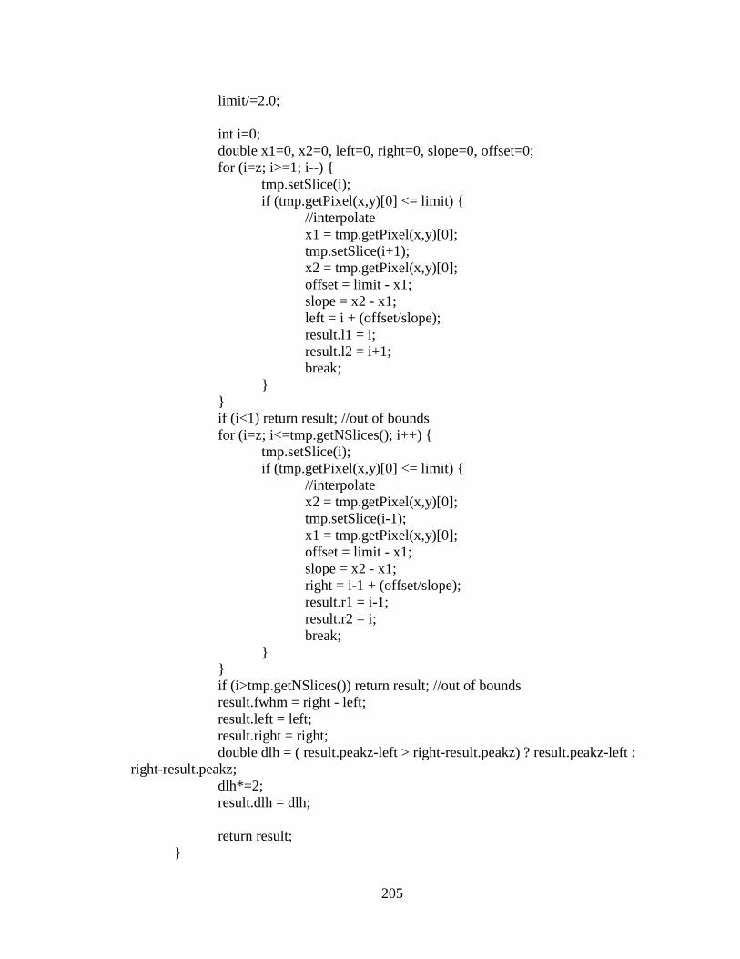
205
limit/=2.0; int i=0; double x1=0, x2=0, left=0, right=0, slope=0, offset=0; for (i=z; i>=1; i--) { tmp.setSlice(i); if (tmp.getPixel(x,y)[0] <= limit) { //interpolate x1 = tmp.getPixel(x,y)[0]; tmp.setSlice(i+1); x2 = tmp.getPixel(x,y)[0]; offset = limit - x1; slope = x2 - x1; left = i + (offset/slope); result.l1 = i; result.l2 = i+1; break; } } if (i<1) return result; //out of bounds for (i=z; i<=tmp.getNSlices(); i++) { tmp.setSlice(i); if (tmp.getPixel(x,y)[0] <= limit) { //interpolate x2 = tmp.getPixel(x,y)[0]; tmp.setSlice(i-1); x1 = tmp.getPixel(x,y)[0]; offset = limit - x1; slope = x2 - x1; right = i-1 + (offset/slope); result.r1 = i-1; result.r2 = i; break; } } if (i>tmp.getNSlices()) return result; //out of bounds result.fwhm = right - left; result.left = left; result.right = right; double dlh = ( result.peakz-left > right-result.peakz) ? result.peakz-left : right-result.peakz; dlh*=2; result.dlh = dlh; return result; }

206
//********************************************************************************* /* peak[0] = x coordinate of peak 0 based peak[1] = y coordinate of peak 0 based peak[2] = z coordinate of peak 1 based peak[3] = peak value */ private Vektor findPeak() { int zmin = imp.getSlice() - planes; int zmax = imp.getSlice() + planes; if (zmin < 1) zmin = 1; if (zmax > imp.getNSlices()) zmax = imp.getNSlices(); //int[] peak = {0,0,0,0}; Vektor peak = new Vektor(); int value = 0; Rectangle bounds = currentRoi.getBounds(); for (int z = zmin; z <= zmax; z++) { imp.setSlice(z); for (int y = (int) bounds.getY(); y <= (int) bounds.getY() + (int) bounds.getHeight(); y++) { for (int x = (int) bounds.getX(); x <= (int) bounds.getX() + (int) bounds.getWidth(); x++) { if (!currentRoi.contains(x,y)) continue; value = (int) integratedIntensity(x,y,z); if ( value > peak.peak ) { peak.x = x; peak.y = y; peak.z = z; peak.peak = value; } } } } return peak; } //********************************************************************************* private int[] fixBounds(ImagePlus tmp, int x, int y, int z) { int[] v = new int[6]; v[0] = x-integratedRadius; v[1] = x+integratedRadius; v[2] = y-integratedRadius;

207
v[3] = y+integratedRadius; v[4] = z-integratedRadius; v[5] = z+integratedRadius; if ( v[0] < 0 ) v[0] = 0; if ( v[2] < 0 ) v[2] = 0; if ( v[4] < 1 ) v[4] = 1; if ( v[1] > imp.getWidth()-1 ) v[1] = imp.getWidth() - 1; if ( v[3] > imp.getHeight()-1 ) v[3] = imp.getHeight() - 1; if ( v[5] > imp.getNSlices() ) v[5] = imp.getNSlices(); return v; } //********************************************************************************* /* private void GaussIt(ImagePlus tmp, double rad) { ImageProcessor ip = tmp.getProcessor(); if (blur == null) blur = new GaussianBlur(); for (int i=1; i<tmp.getNSlices(); i++) { tmp.setSlice(i); blur.blur(ip,rad); } tmp.updateImage(); } */ //********************************************************************************* private double integratedIntensity(int x, int y, int z) { double intensity = 0; voxels = 0; int[] value = {0,0,0,0}; int[] v = fixBounds(imp,x,y,z); int xmin = v[0]; int xmax = v[1]; int ymin = v[2]; int ymax = v[3]; int zmin = v[4]; int zmax = v[5]; for (z = zmin; z <= zmax; z++) { //imp.setSlice(z); imp.setPosition(1,z,1); //imp.setPositionWithoutUpdate(1,z,1); for (y = ymin; y <= ymax; y++) { for (x = xmin; x <= xmax; x++,voxels++) {

208
value = imp.getPixel(x,y); intensity += value[0]; } } } return intensity; } //********************************************************************************* // just needed to avoid abstract class public void lostOwnership(Clipboard clipboard, Transferable contents) {} //********************************************************************************* //odd dimensions only, no funny business private ImagePlus makeSubStack(String name, int x, int y, int zmin, int zmax, int length, int width ) { final int xmin = x-(length/2); //final int xmax = x+(length/2); final int ymin = y-(width/2); //final int ymax = y+(width/2); /* int zmin = z-(depth/2); int zmax = z+(depth/2); if (zmin < 1) { depth-= ( 1-zmin); zmin = 1; } if (zmax > imp.getNSlices()) { depth-=(zmax-imp.getNSlices()); zmax = imp.getNSlices(); } */ ImagePlus tmp = NewImage.createShortImage(name, length, width,zmax-zmin+1, NewImage.FILL_BLACK); ImageProcessor ip = tmp.getProcessor(); int[] data = new int[length*4]; for (int i=zmin,w=1; i<=zmax; i++,w++) { imp.setSlice(i); tmp.setSlice(w); for (int j=0; j<width; j++) { imp.getProcessor().getRow(xmin, j + ymin, data, length);

209
ip.putRow(0,j, data,length); } } tmp.updateImage(); return tmp; } //********************************************************************************* private void measureAll() { RoiManager mgr = RoiManager.getInstance(); if (mgr == null) { IJ.beep(); IJ.showStatus("Roi Manager not open"); return; } Roi[] rois = mgr.getRoisAsArray(); int orig = imp.getSlice(); for (int i=0; i < rois.length; i++) { currentRoi = rois[i]; imp.setSlice(mgr.getSliceNumber(currentRoi.getName())); if (mgr.getSliceNumber(currentRoi.getName()) < 1) { IJ.error("I don't know what the slice is for ROI "+currentRoi.getName()); } measureit(); } imp.setSlice(orig); } //********************************************************************************* private void measureit() { final int orig = imp.getSlice(); try { Vektor peak = findPeak(); Vektor subpeak = new Vektor(); subpeak.x = window/2; subpeak.y = window/2; subpeak.z = range+1; int zmin=peak.z-range; if (zmin<1) zmin = 1; int zmax=peak.z+range;

210
if (zmax>imp.getNSlices()) zmax = imp.getNSlices(); int zpad=0; //if we are too close the front of the stack, we don't pad. if (peak.z-range<1) { subpeak.z = peak.z; } else { zpad = peak.z - range -1; } //ok we know 3x3 and center pixel origImg = makeSubStack("Before",peak.x,peak.y, zmin, zmax, window,window); origResults = findFWHM(subpeak, origImg); if ( rt == null ) { reportCSV(peak,subpeak,zpad); } else { if (rt.getCounter()==0) makeResultTable(); //results table closed reportRT(peak,subpeak,zpad); rt.show("Results Integrated FWHM"); IJ.showStatus(peak.toString()); displayFWHM(peak, subpeak, zmin, zmax, zpad); } origImg.flush(); } catch (Exception e) { } imp.setSlice(orig); } //********************************************************************************* private void makeResultTable() { rt = new ResultsTable(); rt.reset(); rt.getFreeColumn("Cen X"); rt.getFreeColumn("Y"); rt.getFreeColumn("Z"); rt.getFreeColumn("Max"); rt.getFreeColumn("FWHM"); rt.getFreeColumn("DLH"); rt.getFreeColumn("Left");

211
rt.getFreeColumn("Right"); rt.getFreeColumn("Status"); //fields for array of data points } //********************************************************************************* private double validate(double max, Vektor subpeak) { int count=0; for (int z=1; z<=origImg.getNSlices(); z++) { origImg.setSlice(z); if (max == origImg.getPixel(subpeak.x,subpeak.y)[0]) count++; if (count >= flattop) { return 1.0; } } double hmax = origResults.peak/2.0; for (int z=(int) Math.ceil(origResults.left-1); z>0; z--) { origImg.setSlice(z); //IJ.write(String.format("hmax %f > %d at %d starting %f", hmax, filteredImg.getPixel(subpeak[0],subpeak[1])[0], z, filteredResults[1])); if (origImg.getPixel(subpeak.x,subpeak.y)[0] > hmax) { return 2.0; } } for (int z=(int) Math.floor(origResults.right+1); z<origImg.getNSlices(); z++) { origImg.setSlice(z); if (origImg.getPixel(subpeak.x,subpeak.y)[0] > hmax) { return 3.0; } } return 0.0; } //********************************************************************************* public void processWindowEvent(WindowEvent e) { super.processWindowEvent(e); if (e.getID()==WindowEvent.WINDOW_CLOSING) { instance = null; } }
212
//********************************************************************************* private void reportCSV(Vektor peak, Vektor subpeak, int zpad) { try { String s = String.format("%s,%s,%d,%d,%d,%f,%f,%f,%f,%f,%.0f", imp.getTitle(), currentRoi.getName(), peak.x, peak.y, peak.z, origResults.peak, origResults.fwhm, origResults.dlh, origResults.left+zpad, origResults.right+zpad, validate(origResults.peak,subpeak)); for (int z=1; z<=origImg.getNSlices(); z++) { origImg.setSlice(z); s += String.format(",%d",origImg.getPixel(subpeak.x,subpeak.y)[0]); } csvout.write(s); csvout.newLine(); } catch (IOException e) { IJ.write(e.getMessage()); } catch (Exception e) { IJ.write(e.getMessage()); } } //********************************************************************************* private void reportRT(Vektor peak, Vektor subpeak, int zpad) {

213
rt.incrementCounter(); rt.addLabel("Name",currentRoi.getName()); rt.addValue(0,peak.x); //center x rt.addValue(1,peak.y); //center y rt.addValue(2,peak.z); //center z rt.addValue(3,origResults.peak); rt.addValue(4,origResults.fwhm); //fwhm rt.addValue(5,origResults.dlh); //dlh rt.addValue(6,origResults.left+zpad); //left position rt.addValue(7,origResults.right+zpad); //right position rt.addValue(8,validate(origResults.peak,subpeak)); } //********************************************************************************* public void run(String arg) { String options = ""; String csvname = ""; backgroundsubtract = 0; if (IJ.versionLessThan("1.40")) { IJ.showMessage("ImageJ 1.40 or greater required."); return; } if (Macro.getOptions() == null) { makeResultTable(); showDialog(); } else { //validation options = Macro.getOptions(); imp = WindowManager.getCurrentImage(); if (imp == null) return; try { planes = Integer.parseInt(Macro.getValue(options, "planes", "20")); range = Integer.parseInt(Macro.getValue(options, "range", "50")); integratedRadius = Integer.parseInt(Macro.getValue(options, "integratedradius", "1")); flattop = Integer.parseInt(Macro.getValue(options, "flattop", "3")); backgroundsubtract = Integer.parseInt(Macro.getValue(options, "subtract","0")); csvname = Macro.getValue(options, "csv", imp.getTitle()); } catch (NumberFormatException e) {

214
IJ.error("At least one of the arguments is not parseable! " + options); } if (!validateArgs()) return; try { if (!csvname.toLowerCase().endsWith("csv")) csvname += ".csv"; File csv = new File(csvname); csvout = new BufferedWriter(new FileWriter(csv)); csvout.write("planes," + planes + ",range," + range + ",integrated radius," + integratedRadius + ",flat top," + flattop + ",background sub," + backgroundsubtract); csvout.newLine(); csvout.write("image name,region name,x,y,z,max,fwhm,dlh,left,right,status"); for (int i=0; i<(range*2+1); i++) csvout.write(","+i); csvout.newLine(); if (backgroundsubtract>0) //in case pam wants to subtract separately IJ.run("Subtract...", "value="+backgroundsubtract+" stack"); measureAll(); csvout.close(); } catch (Exception e) { CharArrayWriter caw = new CharArrayWriter(); PrintWriter pw = new PrintWriter(caw); e.printStackTrace(pw); IJ.write(caw.toString()); IJ.showStatus(""); } } } //********************************************************************************* private void set_gbc(int row, int column, int width, int height, int fill) { set_gbc(row,column,width,height,fill,0,0); } //********************************************************************************* private void set_gbc(int row, int column, int width, int height, int fill, int padx, int pady) { gbc.gridy = row; gbc.gridx = column;

215
gbc.gridwidth = width; gbc.gridheight = height; gbc.fill = fill; // GridBagConstraints.NONE .HORIZONTAL .VERTICAL .BOTH gbc.ipadx = padx; gbc.ipady = pady; // leave other fields (eg, anchor) unchanged. } //********************************************************************************* private boolean validateArgs() { if (planes < 1) { IJ.showMessage("Invalid number of planes. Try again hoser."); return false; } if (range < 10) { IJ.showMessage("Invalid range to display. Try again hoser."); return false; } if (integratedRadius < 1) { IJ.showMessage("Invalid integrated radius. Try again hoser."); return false; } if (flattop < 2) { IJ.showMessage("Invalid flattop radius. Try again hoser."); return false; } return true; } //********************************************************************************* public void showDialog() { //because windows is stupid setLayout(new FlowLayout()); panel = new Panel(); GridBagLayout gridbag = new GridBagLayout(); panel.setLayout(gridbag); String s = "Select a region around a bead."; Label l = new Label(s); set_gbc(0,0,4,1, GridBagConstraints.HORIZONTAL, 0, 0); gridbag.setConstraints(l,gbc); panel.add(l, gbc); s = "Specify how far above and below to look.";

216
l = new Label(s); set_gbc(1,0,4,1, GridBagConstraints.HORIZONTAL, 0, 0); gridbag.setConstraints(l,gbc); panel.add(l, gbc); s = "Specify the radius to average."; l = new Label(s); set_gbc(2,0,4,1, GridBagConstraints.HORIZONTAL, 0, 10); gridbag.setConstraints(l,gbc); panel.add(l, gbc); l = new Label("Planes to check", Label.RIGHT); set_gbc(3,0,2,1, GridBagConstraints.HORIZONTAL); gridbag.setConstraints(l,gbc); panel.add(l, gbc); txtPlanes = new TextField("20", 20); set_gbc(3,2,2,1, GridBagConstraints.NONE); gridbag.setConstraints(txtPlanes,gbc); panel.add(txtPlanes, gbc); l = new Label("Range to Return", Label.RIGHT); set_gbc(4,0,2,1, GridBagConstraints.HORIZONTAL); gridbag.setConstraints(l,gbc); panel.add(l, gbc); txtRange = new TextField("50", 20); set_gbc(4,2,2,1, GridBagConstraints.NONE); gridbag.setConstraints(txtRange,gbc); panel.add(txtRange, gbc); l = new Label("Integrated Intensity radius", Label.RIGHT); set_gbc(5,0,2,1, GridBagConstraints.HORIZONTAL); gridbag.setConstraints(l,gbc); panel.add(l, gbc); txtIntegratedIntensity = new TextField("1", 20); set_gbc(5,2,2,1, GridBagConstraints.NONE); gridbag.setConstraints(txtIntegratedIntensity,gbc); panel.add(txtIntegratedIntensity, gbc); l = new Label("Flat top pixels", Label.RIGHT); set_gbc(6,0,2,1, GridBagConstraints.HORIZONTAL); gridbag.setConstraints(l,gbc); panel.add(l, gbc); txtFlattop = new TextField("3", 20); set_gbc(6,2,2,1, GridBagConstraints.NONE); gridbag.setConstraints(txtFlattop,gbc); panel.add(txtFlattop, gbc); Button b = new Button("Measure"); b.addActionListener(this); b.addKeyListener(IJ.getInstance()); set_gbc(7,0,1,1, GridBagConstraints.HORIZONTAL); gridbag.setConstraints(b,gbc);

217
panel.add(b); b = new Button("Measure All"); b.addActionListener(this); b.addKeyListener(IJ.getInstance()); set_gbc(7,1,1,1, GridBagConstraints.HORIZONTAL); gridbag.setConstraints(b,gbc); panel.add(b); b = new Button("Dump ROI"); b.addActionListener(this); b.addKeyListener(IJ.getInstance()); set_gbc(7,2,1,1, GridBagConstraints.HORIZONTAL); gridbag.setConstraints(b,gbc); panel.add(b); b = new Button("Clear ROI"); b.addActionListener(this); b.addKeyListener(IJ.getInstance()); set_gbc(7,3,1,1, GridBagConstraints.HORIZONTAL); gridbag.setConstraints(b,gbc); panel.add(b); b = new Button("Copy Values"); b.addActionListener(this); b.addKeyListener(IJ.getInstance()); set_gbc(8,0,1,1, GridBagConstraints.NONE); gridbag.setConstraints(b,gbc); panel.add(b); b = new Button("Check Outlier"); b.addActionListener(this); b.addKeyListener(IJ.getInstance()); set_gbc(8,1,1,1, GridBagConstraints.NONE); gridbag.setConstraints(b,gbc); panel.add(b); l = new Label("Status:"); set_gbc(9,0,2,1, GridBagConstraints.HORIZONTAL); gridbag.setConstraints(l,gbc); panel.add(l, gbc); l = new Label("0 - valid"); set_gbc(10,0,2,1, GridBagConstraints.HORIZONTAL); gridbag.setConstraints(l,gbc); panel.add(l, gbc); l = new Label("Blue - original values"); set_gbc(10,2,2,1, GridBagConstraints.HORIZONTAL); gridbag.setConstraints(l,gbc); panel.add(l, gbc); l = new Label("1 - flat top"); set_gbc(11,0,2,1, GridBagConstraints.HORIZONTAL); gridbag.setConstraints(l,gbc);

218
panel.add(l, gbc); l = new Label("Orange - mean of integrated"); set_gbc(11,2,2,1, GridBagConstraints.HORIZONTAL); gridbag.setConstraints(l,gbc); panel.add(l, gbc); l = new Label("2 - noisy left of peak"); set_gbc(12,0,2,1, GridBagConstraints.HORIZONTAL); gridbag.setConstraints(l,gbc); panel.add(l, gbc); l = new Label("3 - noisy right of peak"); set_gbc(13,0,2,1, GridBagConstraints.HORIZONTAL); gridbag.setConstraints(l,gbc); panel.add(l, gbc); add(panel); pack(); GUI.center(this); setVisible(true); } //********************************************************************************* void showAbout() { String title = "About " + getClass().getName() + "..."; IJ.showMessage(title, "This app takes a region, finds the brightest point and averages it with pixels in a radius of x."); } //********************************************************************************* void error() { IJ.showMessage(getClass().getName(), "This plugin requires a definied region to work"); } }

219
C. Excel macros
1. Common_Tools Option Explicit Public WSColl As Collection Public CHColl As Collection Public Const c_badpoint As Integer = 6 Public Const c_saturated As Integer = 3 Public Const c_pamdecide As Integer = 7 Public Const c_dontgraph As Integer = 15 Const c_name As Integer = 1 Const c_roi As Integer = 2 Const c_z As Integer = 8 Const c_meanbkg As Integer = 13 Sub StopAllEvents() ''' There are problems with out of control event cascades Application.EnableEvents = False 'Your code here. Application.EnableEvents = True End Sub Sub stop_excel(control As IRibbonControl) ''' Disable the GUI so an event cascade isn't triggered ''' control is not used Application.EnableEvents = False Application.ScreenUpdating = False Application.DisplayAlerts = False End Sub Sub start_excel(control As IRibbonControl) ''' Enables the GUI to process user events ''' control is not used Application.EnableEvents = True Application.ScreenUpdating = True Application.DisplayAlerts = True End Sub Private Sub BuildCustomMenu() ''' This adds the right click functionality of the plugin. ''' At the moment that is just the ability to remove and restore rows from the processed sheet.s

220
Dim ctrl As CommandBarControl Dim btn As CommandBarControl Dim i As Integer 'add a 'popup' control to the cell commandbar (menu) Set ctrl = Application.CommandBars("Cell").Controls.Add(Type:=msoControlButton, Before:=1, Temporary:=True) ctrl.Caption = "Remove row" ctrl.OnAction = "remove_row" Set ctrl = Application.CommandBars("Cell").Controls.Add(Type:=msoControlButton, Before:=2, Temporary:=True) ctrl.Caption = "Restore row" ctrl.OnAction = "restore_row" Set ctrl = Application.CommandBars("Row").Controls.Add(Type:=msoControlButton, Before:=1, Temporary:=True) ctrl.Caption = "Remove row" ctrl.OnAction = "remove_row" Set ctrl = Application.CommandBars("Row").Controls.Add(Type:=msoControlButton, Before:=2, Temporary:=True) ctrl.Caption = "Restore row" ctrl.OnAction = "restore_row" End Sub Private Sub DeleteCustomMenu() ''' This goes through and removes any additions to the right click menus. ''' It is used to prevent duplicate entries and cleanup. Dim ctrl As CommandBarControl 'go thru all the cell commandbar controls and delete our menu item For Each ctrl In Application.CommandBars("Cell").Controls If ctrl.Caption = "Restore row" Or _ ctrl.Caption = "Remove row" Then ctrl.Delete End If Next For Each ctrl In Application.CommandBars("Row").Controls If ctrl.Caption = "Restore row" Or _ ctrl.Caption = "Remove row" Then ctrl.Delete End If Next End Sub Function GetRolling(arr As Range, low As Double, high As Double, zmicrons As Integer, col As Integer)

221
Dim rw As Range Dim count, i As Integer Dim total As Double Dim currentUpdating As Boolean currentUpdating = Application.ScreenUpdating Application.ScreenUpdating = False Application.DisplayAlerts = False total = 0 count = 0 ' count points For i = arr.Row To arr.Row + arr.Rows.count - 1 If Cells(i, zmicrons).value >= low And Cells(i, zmicrons).value < high Then total = total + Cells(i, col).value count = count + 1 End If Next i If count < 1 Then GetRolling = 0 Else GetRolling = total / count End If Application.ScreenUpdating = currentUpdating Application.DisplayAlerts = True End Function Function GetRollingStdev(arr As Range, low As Double, high As Double, zmicrons As Integer, col As Integer, meancol As Range) Dim count, i As Integer Dim total As Double Dim currentUpdating As Boolean currentUpdating = Application.ScreenUpdating Application.ScreenUpdating = False Application.DisplayAlerts = False total = 0 count = 0 ' count points For i = arr.Row To arr.Row + arr.Rows.count - 1 If Cells(i, zmicrons).value >= low And Cells(i, zmicrons).value < high Then total = total + (Cells(i, col).value - meancol.value) ^ 2 count = count + 1 End If
222
Next i If count < 2 Then GetRollingStdev = 0 Else GetRollingStdev = Sqr(total / (count - 1)) End If Application.ScreenUpdating = currentUpdating Application.DisplayAlerts = True End Function Function GetTTest(arr As Range, fwhm As Range, rolling As Range, stdev As Range) Dim t As Double If stdev.value <> 0 Then ' t test t = Abs(fwhm.value - rolling.value) / stdev.value If count < 3 Then Cells(fwhm.Row, c_resttest).Interior.ColorIndex = c_dontgraph ElseIf count > 147 And t >= Sheets("ASTM").Cells(Application.Min(count, 147) - 1, 3).value Then Cells(fwhm.Row, c_resttest).Interior.ColorIndex = c_pamdecide ElseIf t >= Sheets("ASTM").Cells(Application.Min(count, 147) - 1, 3).value Then Cells(fwhm.Row, c_resttest).Interior.ColorIndex = c_badpoint Else Cells(fwhm.Row, c_resttest).Interior.ColorIndex = 0 End If Else Cells(fwhm.Row, c_resttest).Interior.ColorIndex = c_badpoint End If GetTTest = t End Function ' Because excel screws this up a disturbing amount of the time! Function GetStopRow(ByVal start_row As Integer) Dim i As Integer Dim s As String i = start_row s = Cells(i, 1).value Do i = i + 1 Loop Until (s <> Cells(i, 1)) Or (i > ActiveSheet.UsedRange.Rows.count) GetStopRow = i - 1 End Function ' flag row in raw sheet Function highlight_and_delete_row(arr As Range, color As Integer) As Boolean

223
Dim j As Integer Dim name, roi As String highlight_and_delete_row = False name = arr.Cells(1, 1).value roi = arr.Cells(1, 2).value For j = 3 To Sheets("Raw").UsedRange.Rows.count If Sheets("Raw").Cells(j, 1).value = name And Sheets("Raw").Cells(j, 2).value = roi Then Range(Sheets("Raw").Cells(j, 1), Sheets("Raw").Cells(j, 26)).Interior.ColorIndex = color GoTo FOUND_IT End If Next j MsgBox arr.Address & " cannot be found in the raw sheet" Exit Function FOUND_IT: arr.Rows(1).EntireRow.Delete highlight_and_delete_row = True End Function Public Function MyDocsPath() As String MyDocsPath = Environ$("USERPROFILE") & "\My Documents\" End Function Sub remove_row() If (ActiveSheet.name <> "Processed" And ActiveSheet.name <> "Binning") Or Selection.Rows.count < 1 Then Exit Sub End If Dim currentUpdating As Boolean currentUpdating = Application.ScreenUpdating Application.ScreenUpdating = False Application.DisplayAlerts = False Dim color As Integer Dim cl As Range Dim i, first, last As Integer ' loop rows first = Selection.Row last = Selection.Row + Selection.Rows.count - 1

224
For i = first To last ' find color For Each cl In Cells(first, c_name).EntireRow.Cells If cl.Interior.ColorIndex > 0 Then color = cl.Interior.ColorIndex GoTo FOUND_COLOR End If Next cl color = c_badpoint FOUND_COLOR: Call highlight_and_delete_row(Cells(first, c_name).EntireRow, color) Next i Application.ScreenUpdating = currentUpdating Application.DisplayAlerts = False End Sub Sub restore_row() If ActiveSheet.name <> "Raw" Or Selection.Rows.count < 1 Then Exit Sub End If ' find the sample in processed Dim j, first, last As Integer Dim name, roi As String Dim arr, src As Range Dim raw, processed As Worksheet Dim currentUpdating As Boolean currentUpdating = Application.ScreenUpdating Application.ScreenUpdating = False Application.DisplayAlerts = False Set raw = Sheets("Raw") Set processed = Sheets("Processed") Set src = Selection.Rows(1).EntireRow name = src.Cells(1, c_name).value roi = src.Cells(1, c_roi).value first = 0 last = 0 For j = 3 To processed.UsedRange.Rows.count If processed.Cells(j, c_name).value = name Then first = j GoTo FOUND_BEGINNING End If Next j

225
FOUND_BEGINNING: For j = first + 1 To processed.UsedRange.Rows.count If processed.Cells(j, c_name).value <> name Then last = j - 1 GoTo FOUND_END End If Next j FOUND_END: Set arr = Range(Cells(first, c_name), Cells(last, 26)) ' insert row at end of sample in processed last = last + 1 processed.Rows(last).EntireRow.Insert processed.Rows(last).EntireRow.value = src.value 'processed.Range(processed.Cells(last, c_name), processed.Cells(last, c_meanbkg)).Interior.ColorIndex = 40 ' resort the sample Debug.Print "sorting " & first & " " & last With processed.Sort .SortFields.Clear .SortFields.Add Key:=Range(processed.Cells(first, c_z), processed.Cells(last, c_z)), _ SortOn:=xlSortOnValues, Order:=xlAscending, DataOption:=xlSortTextAsNumbers .SetRange Range(processed.Cells(first, c_name), processed.Cells(last, c_meanbkg)) .Header = xlNo .Orientation = xlTopToBottom .SortMethod = xlPinYin .Apply End With ' Plug in all the stats stuff Call Stat_Columns(first, last) Application.ScreenUpdating = currentUpdating Application.DisplayAlerts = True raw.Activate End Sub Sub Ribbon_Loaded(ribbon As IRibbonUI) ' put everything to do on startup here! Call DeleteCustomMenu Call BuildCustomMenu End Sub Sub Setup_Workbook() Dim currentUpdating As Boolean Dim i As Integer Dim s As Worksheet

226
Dim tmp As Workbook Dim WSObj As CWorksheetObject Set WSObj = New CWorksheetObject Set WSColl = New Collection currentUpdating = Application.ScreenUpdating Application.ScreenUpdating = False Application.DisplayAlerts = False If Workbooks.count = 0 Then Set tmp = Workbooks.Add tmp.Title = "Analysis" End If Sheets.Add after:=Worksheets(Worksheets.count) Sheets.Add after:=Worksheets(Worksheets.count) Sheets.Add after:=Worksheets(Worksheets.count) Sheets.Add after:=Worksheets(Worksheets.count) For i = ActiveWorkbook.Worksheets.count - 4 To 1 Step -1 Worksheets(i).Delete Next i Set s = Sheets(1) s.name = "Raw" Set s = Sheets(2) s.name = "Processed" Set WSObj.WS = s WSColl.Add Item:=WSObj, Key:=s.name Set s = Sheets(3) s.name = "ASTM" Set s = Sheets(4) s.name = "Binning" Application.DisplayAlerts = False Application.ScreenUpdating = currentUpdating End Sub Sub UnSelectActiveCell() Dim Rng As Range Dim FullRange As Range If Selection.Cells.count > 1 Then For Each Rng In Selection.Cells If Rng.Address <> ActiveCell.Address Then

227
If FullRange Is Nothing Then Set FullRange = Rng Else Set FullRange = Application.Union(FullRange, Rng) End If End If Next Rng If FullRange.Cells.count > 0 Then FullRange.Select End If End If End Sub
2. Pam_Tools Option Explicit Const c_name As Integer = 1 Const c_roi As Integer = 2 Const c_hot3x3 As Integer = 3 Const c_hotpixel As Integer = 4 Const c_multiple As Integer = 5 Const c_x As Integer = 6 Const c_y As Integer = 7 Const c_z As Integer = 8 Const c_mean As Integer = 9 Const c_meanstdev As Integer = 10 Const c_background As Integer = 11 Const c_backgroundstdev As Integer = 12 Const c_meanbkg As Integer = 13 Const c_intensityerror As Integer = 14 Const c_offset As Integer = 15 Const c_offsetstdev As Integer = 16 Const c_zmicrons As Integer = 17 Const c_zerror As Integer = 18 Const c_count As Integer = 19 Const c_rollingz As Integer = 20 Const c_rollingzstdev As Integer = 21 Const c_ttest As Integer = 22 Const c_smoothedz As Integer = 23 Const c_smoothedcount As Integer = 24 Const c_graph_zmicrons As Integer = 26 Const c_graph_meanbkg As Integer = 27

228
Const c_graph_rollingz As Integer = 28 Const c_avgz As Integer = 30 Const c_avgmeanbkg As Integer = 31 Const c_stdevz As Integer = 32 Const c_stdevmeanbkg As Integer = 33 Const c_minz As Integer = 34 Const c_maxz As Integer = 35 Public smite As Boolean Sub smite_status(control As IRibbonControl, state As Boolean) smite = state End Sub Sub addToolBar(ByVal barName As String) Dim bar As CommandBar On Error Resume Next Set bar = Application.CommandBars(barName) If Not bar Is Nothing Then Application.CommandBars(barName).Delete End If Set bar = Application.CommandBars.Add(barName, Position:=msoBarFloating, Temporary:=True) End Sub 'Private Sub ThisAddIn_Shutdown(ByVal sender As Object, ByVal e As System.EventArgs) Handles Me.Shutdown ' Application.CommandBars("Monte Carlo").Delete() 'End Sub ' This is just a stub show I can pick icons easier Sub Show_icons() Dim oToolbar As CommandBar Dim oButton As CommandBarButton Dim MyToolbar As String Dim i As Integer ' Give the toolbar a name MyToolbar = "Icon List" ' First, delete the toolbar if it already exists 'On Error Resume Next ' so that it doesn't stop on the next line if the toolbar's already there

229
' Build the command bar addToolBar (MyToolbar) Set oToolbar = Application.CommandBars(MyToolbar) 'Set oToolbar = CommandBars.Add(Name:=MyToolbar, Position:=msoBarFloating, Temporary:=True) If Err.Number <> 0 Then ' Probably means the toolbar's already there, so we have nothing to do Debug.Print Err.Number & " " & Err.Description Exit Sub End If On Error GoTo ErrorHandler ' loop adding buttons For i = 1 To 255 Set oButton = oToolbar.Controls.Add(Type:=msoControlButton) ' And set some of the button's properties With oButton .DescriptionText = "Merge a folder of CSVs into 1 sheet" 'Tooltip text when mouse if placed over button .Caption = "" & i 'Text if Text in Icon is chosen .Style = msoButtonIcon ' Button displays as icon, not text or both .FaceId = i '52 is my favorite pig; chooses icon #52 from the available Office icons End With Next i oToolbar.Visible = True NormalExit: Exit Sub ' so it doesn't go on to run the errorhandler code ErrorHandler: 'Just in case there is an error Debug.Print Err.Number & vbCrLf & Err.Description Resume NormalExit: End Sub ' Merge csv and generate sheets for Pam ' from the Dark Lord of Information ' 'Sub Auto_Open() ' Dim oToolbar As CommandBar

230
' Dim oButton As CommandBarButton ' Dim MyToolbar As String ' Give the toolbar a name ' MyToolbar = "Pam Tools" ' First, delete the toolbar if it already exists ' On Error Resume Next ' so that it doesn't stop on the next line if the toolbar's already there ' Build the command bar ' Build the command bar ' addToolBar (MyToolbar) ' Set oToolbar = Application.CommandBars(MyToolbar) ' If Err.Number <> 0 Then ' Probably means the toolbar's already there, so we have nothing to do ' Debug.Print Err.Number & " " & Err.Description ' Exit Sub ' End If ' On Error GoTo ErrorHandler ' Now add a button to the new toolbar ' Set oButton = oToolbar.Controls.Add(Type:=msoControlButton) ' And set some of the button's properties ' With oButton ' .DescriptionText = "Merge a folder of CSVs into 1 sheet" 'Tooltip text when mouse if placed over button ' .Caption = "Merge CSVs" 'Text if Text in Icon is chosen ' .OnAction = "mergeCSVs" 'Runs the Sub Button1() code when clicked ' .Style = msoButtonIcon ' Button displays as icon, not text or both ' .FaceId = 23 '52 is my favorite pig; chooses icon #52 from the available Office icons ' End With ' Now add a button to the new toolbar ' Set oButton = oToolbar.Controls.Add(Type:=msoControlButton) ' And set some of the button's properties ' With oButton ' .DescriptionText = "Sort, remove maxxed, and compute common parameters" 'Tooltip text when mouse if placed over button ' .Caption = "Prune" 'Text if Text in Icon is chosen ' .OnAction = "prune" 'Runs the Sub Button1() code when clicked ' .Style = msoButtonIcon ' Button displays as icon, not text or both

231
' .FaceId = 108 ' End With ' Now add a button to the new toolbar ' Set oButton = oToolbar.Controls.Add(Type:=msoControlButton) ' And set some of the button's properties ' With oButton ' .DescriptionText = "Group beads according to depth" 'Tooltip text when mouse if placed over button ' .Caption = "Binning" 'Text if Text in Icon is chosen ' .OnAction = "fruitcake" 'Runs the Sub Button1() code when clicked ' .Style = msoButtonIcon ' Button displays as icon, not text or both ' .FaceId = 107 ' End With ' Set oButton = oToolbar.Controls.Add(Type:=msoControlButton) ' And set some of the button's properties ' With oButton ' .DescriptionText = "Group beads according to depth" 'Tooltip text when mouse if placed over button ' .Caption = "Graphs" 'Text if Text in Icon is chosen ' .OnAction = "graphs" 'Runs the Sub Button1() code when clicked ' .Style = msoButtonIcon ' Button displays as icon, not text or both ' .FaceId = 17 ' End With ' You can set the toolbar position and visibility here if you like ' By default, it'll be visible when created ' oToolbar.Top = 150 ' oToolbar.Left = 150 ' oToolbar.Visible = True 'NormalExit: ' Exit Sub ' so it doesn't go on to run the errorhandler code 'ErrorHandler: 'Just in case there is an error ' MsgBox Err.Number & vbCrLf & Err.Description ' Resume NormalExit: 'End Sub Sub fruitcake(control As IRibbonControl) Dim free_col, i, j, k As Integer Dim processed As Worksheet

232
Set processed = Worksheets(2) Dim currentUpdating As Boolean currentUpdating = Application.ScreenUpdating Application.ScreenUpdating = False Application.DisplayAlerts = False free_col = processed.UsedRange.Columns.count + 2 Cells(1, free_col).Select ActiveCell.value = "binning" Cells(2, free_col).Select ActiveCell.value = "z (microns)" Cells(2, free_col + 1).Select ActiveCell.value = "z avg" Cells(2, free_col + 2).Select ActiveCell.value = "z stdev" Cells(2, free_col + 3).Select ActiveCell.value = "z error" Cells(2, free_col + 4).Select ActiveCell.value = "z error total" Cells(2, free_col + 5).Select ActiveCell.value = "intensity" Cells(2, free_col + 6).Select ActiveCell.value = "intensity stdev" Cells(2, free_col + 7).Select ActiveCell.value = "intensity error" Cells(2, free_col + 8).Select ActiveCell.value = "total intensity error" Cells(2, free_col + 9).Select ActiveCell.value = "count" Dim start_row, stop_row, last_row As Integer Dim low, high As Double Dim arr As Range start_row = 3 stop_row = processed.UsedRange.Rows.count k = start_row For j = 0 To 150 Step 5 Cells(k, free_col).value = j If j = 0 Then low = -100 Else low = j - 2.5 End If

233
If j = 150 Then high = 1000 Else high = j + 2.5 End If Set arr = ActiveSheet.Range(Cells(start_row, c_zmicrons), Cells(stop_row, c_zmicrons)) Cells(k, free_col + 1).Select ActiveCell.Formula = "=GetZAvg(" & arr.Address & "," & low & "," & high & ")" Cells(k, free_col + 2).Select ActiveCell.Formula = "=GetZStdev(" & arr.Address & "," & low & "," & high & ")" Cells(k, free_col + 3).Select Set arr = ActiveSheet.Range(Cells(start_row, c_zmicrons), Cells(stop_row, c_zerror)) ActiveCell.Formula = "=GetZError(" & arr.Address & "," & low & "," & high & ")" Cells(k, free_col + 4).Select ActiveCell.Formula = "=iferror(sqrt(V$" & k & "^2 + W$" & k & "^2)," & Chr(34) & "undefinied" & Chr(34) & ")" Cells(k, free_col + 5).Select Set arr = ActiveSheet.Range(Cells(start_row, c_mean), Cells(stop_row, c_zmicrons)) ActiveCell.Formula = "=GetIntensity(" & arr.Address & "," & low & "," & high & ")" Cells(k, free_col + 6).Select ActiveCell.Formula = "=GetIntensityStdev(" & arr.Address & "," & low & "," & high & ")" Cells(k, free_col + 7).Select Set arr = ActiveSheet.Range(Cells(start_row, c_intensityerror), Cells(stop_row, c_zmicrons)) ActiveCell.Formula = "=GetIntensityError(" & arr.Address & "," & low & "," & high & ")" Cells(k, free_col + 8).Select ActiveCell.Formula = "=iferror(sqrt(Z$" & k & "^2 + AA$" & k & "^2)," & Chr(34) & "undefinied" & Chr(34) & ")" Cells(k, free_col + 9).Select Set arr = ActiveSheet.Range(Cells(start_row, c_zmicrons), Cells(stop_row, c_zmicrons)) ActiveCell.Formula = "=GetCount(" & arr.Address & "," & low & "," & high & ")" k = k + 1 Next j Application.ScreenUpdating = False Application.DisplayAlerts = currentUpdating End Sub

234
Sub graph(control As IRibbonControl) Dim arr As Range Dim dst, xaxis, meanbkg As Range Dim current, i, start_row, stop_row As Long Dim zlimit As Double Dim currentUpdating As Boolean currentUpdating = Application.ScreenUpdating Application.ScreenUpdating = False Application.DisplayAlerts = False 'Application.EnableEvents = False 'copy current = 3 stop_row = ActiveSheet.UsedRange.Rows.count For i = 3 To stop_row If (Cells(i, c_ttest).Interior.ColorIndex < 1 Or Cells(i, c_ttest).Interior.ColorIndex = c_dontgraph) Then Cells(current, c_graph_zmicrons).value = Cells(i, c_zmicrons).value Cells(current, c_graph_meanbkg).value = Cells(i, c_meanbkg).value Cells(current, c_graph_rollingz).value = Cells(i, c_smoothedz).value current = current + 1 End If Next i Set arr = Range(Cells(3, c_zmicrons), Cells(stop_row, c_zmicrons)) Set dst = Range(Cells(3, c_graph_zmicrons), Cells(stop_row, c_graph_zmicrons)) 'dst.value = arr.value Set xaxis = dst Set arr = Range(Cells(3, c_meanbkg), Cells(stop_row, c_meanbkg)) Set dst = Range(Cells(3, c_graph_meanbkg), Cells(stop_row, c_graph_meanbkg)) 'dst.value = arr.value Set meanbkg = dst Set arr = Range(Cells(3, c_smoothedz), Cells(stop_row, c_smoothedz)) Set dst = Range(Cells(3, c_graph_rollingz), Cells(stop_row, c_graph_rollingz)) 'dst.value = arr.value stop_row = current 'sort With ActiveSheet.Sort .SortFields.Clear .SortFields.Add Key:=Range(Cells(3, c_graph_zmicrons), Cells(stop_row, c_graph_zmicrons)), _ SortOn:=xlSortOnValues, Order:=xlAscending, DataOption:=xlSortTextAsNumbers .SetRange Range(Cells(3, c_graph_zmicrons), Cells(stop_row, c_graph_rollingz)) .Header = xlNo .Orientation = xlTopToBottom

235
.SortMethod = xlPinYin .Apply End With ' find start_row based on Z criteria! start_row = 3 ' idiot check If Not IsNumeric(Cells(1, c_stdevmeanbkg).value) Or IsEmpty(Cells(1, c_stdevmeanbkg).value) Then MsgBox "Error: Graph from Z must be a number!" Exit Sub End If zlimit = Cells(1, c_stdevmeanbkg).value For start_row = 3 To stop_row If Cells(start_row, c_graph_zmicrons).value >= zlimit Then Exit For End If Next start_row 'generate extra averaged stuff Debug.Print "Start row " & start_row Set arr = Range(Cells(start_row, c_graph_rollingz), Cells(stop_row, c_graph_rollingz)) Call BinZ(arr) 'graph Dim CHObj As MyChartObject Set CHObj = New MyChartObject Set CHColl = New Collection Range(Cells(start_row, c_graph_zmicrons), Cells(stop_row, 28)).Activate ActiveSheet.Shapes.AddChart(Excel.XlChartType.xlXYScatter).Select Set CHObj.CO = ActiveChart Debug.Print ActiveChart.name CHColl.Add Item:=CHObj, Key:=ActiveChart.name Set xaxis = Range(Cells(start_row, c_graph_zmicrons), Cells(stop_row, c_graph_zmicrons)) Set meanbkg = Range(Cells(start_row, c_graph_meanbkg), Cells(stop_row, c_graph_meanbkg)) Set dst = Range(Cells(start_row, c_graph_rollingz), Cells(stop_row, c_graph_rollingz)) 'ActiveChart.SeriesCollection.NewSeries

236
ActiveChart.SeriesCollection(1).name = "=""mean-background""" ActiveChart.SeriesCollection(1).XValues = xaxis ActiveChart.SeriesCollection(1).Values = meanbkg 'ActiveChart.SeriesCollection.NewSeries ActiveChart.SeriesCollection(2).name = "=""smoothed Z""" ActiveChart.SeriesCollection(2).XValues = xaxis ActiveChart.SeriesCollection(2).Values = dst ActiveChart.SeriesCollection(1).Select With Selection .MarkerStyle = xlMarkerStyleDiamond .MarkerSize = 2 End With ActiveChart.SeriesCollection(2).Select With Selection .MarkerStyle = 1 .MarkerSize = 2 End With ActiveChart.Axes(xlCategory).MinimumScale = 0 Dim offset As Integer offset = ActiveChart.Parent.Top + ActiveChart.Parent.Height + 50 ' chart 2.0 Set CHObj = New MyChartObject Set CHColl = New Collection Range(Cells(start_row, c_graph_zmicrons), Cells(stop_row, c_graph_rollingz)).Activate ActiveSheet.Shapes.AddChart(Excel.XlChartType.xlXYScatter).Select Set CHObj.CO = ActiveChart Debug.Print ActiveChart.name CHColl.Add Item:=CHObj, Key:=ActiveChart.name ActiveChart.SeriesCollection(1).name = "=""mean-background""" ActiveChart.SeriesCollection(1).XValues = xaxis ActiveChart.SeriesCollection(1).Values = meanbkg Set xaxis = Range(Cells(3, c_avgz), Cells(Range(Cells(65536, c_avgz).Address).End(xlUp).Row, c_avgz)) Set dst = Range(Cells(3, c_avgmeanbkg), Cells(Range(Cells(65536, c_avgmeanbkg).Address).End(xlUp).Row, c_avgmeanbkg)) ActiveChart.SeriesCollection(2).name = "=""Averaged Z""" ActiveChart.SeriesCollection(2).XValues = xaxis ActiveChart.SeriesCollection(2).Values = dst ActiveChart.SeriesCollection(1).Select

237
With Selection .MarkerStyle = xlMarkerStyleDiamond .MarkerSize = 2 End With ActiveChart.SeriesCollection(2).Select With Selection .MarkerStyle = 1 .MarkerSize = 2 End With ActiveChart.Axes(xlCategory).MinimumScale = 0 ActiveChart.Parent.Top = offset Application.ScreenUpdating = currentUpdating Application.DisplayAlerts = True Application.EnableEvents = False End Sub Sub highlight_outliers_4095() Dim raw As Worksheet Dim rw As Range Dim currentUpdating As Boolean currentUpdating = Application.ScreenUpdating Application.ScreenUpdating = False Application.DisplayAlerts = False Set raw = Worksheets(1) For Each rw In raw.UsedRange.Rows If Cells(rw.Row, 3).value >= 4095 And IsNumeric(Cells(rw.Row, 3).value) Then rw.EntireRow.Interior.ColorIndex = c_saturated End If Next rw Application.ScreenUpdating = currentUpdating Application.DisplayAlerts = True End Sub Sub MergeCSVs(control As IRibbonControl) On Error GoTo SMACK_PAM Dim planes, radius As Integer Dim currentUpdating As Boolean Dim folderName As Variant Dim cell_to_paste_next_dataset As Range Dim active_workbook, dataset_workbook As Workbook Dim active_sheet As Worksheet planes = 0

238
radius = 0 'Get folder Dim fd As FileDialog Set fd = Application.FileDialog(msoFileDialogFolderPicker) With fd If .Show = -1 Then folderName = .SelectedItems.Item(1) Else Exit Sub End If End With Set fd = Nothing Call Setup_Workbook 'Lists all the files in the current directory Set cell_to_paste_next_dataset = Cells(1, 1) Set active_workbook = ActiveWorkbook Set active_sheet = Sheets("Raw") Dim fool As String currentUpdating = Application.ScreenUpdating Application.ScreenUpdating = False Application.DisplayAlerts = False Debug.Print (folderName & "*.csv") fool = Dir(folderName & "\\*.csv") Dim paste_row As Integer paste_row = 1 ' so I don't skip the first row... Do While fool <> vbNullString Debug.Print fool If active_workbook.name <> fool And fool <> "" Then Workbooks.Open Filename:=folderName & "\" & fool Set dataset_workbook = ActiveWorkbook ' valid same parameters before adding! If (planes <> 0) Then If planes <> Cells(1, 2).value Or radius <> Cells(1, 4).value Then MsgBox ("File " & fool & " has different processing parameters. Ignoring!") fool = Dir GoTo OOPS End If Else planes = Cells(1, 2).value radius = Cells(1, 4).value End If

239
Range(ActiveCell.SpecialCells(xlLastCell), Cells(1)).Copy active_sheet.Activate Cells(paste_row, 1).Select ActiveSheet.Paste dataset_workbook.Close paste_row = ActiveCell.SpecialCells(xlLastCell).Row + 1 End If OOPS: fool = Dir Loop ' bring in T test chart! Set active_sheet = Sheets("ASTM") Debug.Print MyDocsPath & "astm.xlsx" Workbooks.Open Filename:=MyDocsPath & "astm.xlsx" Set dataset_workbook = ActiveWorkbook Range(ActiveCell.SpecialCells(xlLastCell), Cells(1)).Copy active_sheet.Activate Cells(1, 1).Select ActiveSheet.Paste dataset_workbook.Close paste_row = ActiveCell.SpecialCells(xlLastCell).Row + 1 Sheets("Raw").Activate Call highlight_outliers_4095 Debug.Print planes & " " & radius Application.DisplayAlerts = True Application.ScreenUpdating = currentUpdating Call UnSelectActiveCell Exit Sub SMACK_PAM: MsgBox "Put the astm.xlsx file in your My Documents folder!" End Sub Sub process_merged(control As IRibbonControl) Dim currentUpdating As Boolean Dim source, processing As Worksheet Dim i As Integer Set source = Worksheets(1) Set processing = Worksheets(2) currentUpdating = Application.ScreenUpdating Application.ScreenUpdating = False Application.DisplayAlerts = False source.Activate

240
Range(ActiveCell.SpecialCells(xlLastCell), Cells(1)).Copy processing.Activate Cells(1, 1).Select ActiveSheet.Paste i = 3 ' remove dupe captions Do If Cells(i, 1).value Like "planes" Or Cells(i, 1).value Like "image name" Then processing.Rows(i).EntireRow.Delete Else i = i + 1 End If Loop Until (i > processing.UsedRange.Rows.count Or IsEmpty(Cells(i, 1).value)) i = 3 ' remove pegged rows Do If Cells(i, 3).value >= 4095 Then processing.Rows(i).EntireRow.Delete Else i = i + 1 End If Loop Until i > processing.UsedRange.Rows.count ' assign sort column 'hint_col = processing.UsedRange.Columns.count + 2 'Cells(3, hint_col).Select 'ActiveCell.Formula = "=GetElement(B3,1,""-"")" 'ActiveCell.FormulaR1C1 = "=GetElement(RC[-13],3,""-"")" 'ActiveCell.AutoFill Range(ActiveCell, Cells(processing.UsedRange.Rows.count, ActiveCell.Column)) ' sort ranges Dim start_row, stop_row As Integer i = 3 Do start_row = i stop_row = GetStopRow(start_row) i = stop_row + 1 Debug.Print start_row & " " & stop_row With processing.Sort .SortFields.Clear .SortFields.Add Key:=Range(Cells(start_row, c_z), Cells(stop_row, c_z)), _ SortOn:=xlSortOnValues, Order:=xlAscending, DataOption:=xlSortTextAsNumbers

241
.SetRange Range(Cells(start_row, 1), Cells(stop_row, c_meanbkg)) .Header = xlNo .Orientation = xlTopToBottom .SortMethod = xlPinYin .Apply End With Loop Until i > processing.UsedRange.Rows.count 'processing.Columns(hint_col).EntireColumn.Delete processing.Activate Application.ScreenUpdating = currentUpdating Application.DisplayAlerts = True Call Stat_Columns(3, processing.UsedRange.Rows.count) Call UnSelectActiveCell End Sub Sub Label_Columns() Cells(2, c_intensityerror).value = "intensity error" Cells(2, c_offset).value = "offset" Cells(2, c_offsetstdev).value = "offset stdev" Cells(2, c_zmicrons).value = "z (microns)" Cells(2, c_zerror).value = "z error" Cells(2, c_count).value = "count" Cells(2, c_rollingz).value = "Rolling Z" Cells(2, c_rollingzstdev).value = "Rolling Z Stdev" Cells(2, c_ttest).value = "T Test" Cells(2, c_smoothedz).value = "Smoothed Z" Cells(2, c_smoothedcount).value = "Smoothed Count" Cells(1, c_ttest).value = "Fudge" Cells(1, c_smoothedz).Select If (IsEmpty(ActiveCell.value)) Then ActiveCell.value = 5 Cells(2, c_graph_zmicrons).Select ActiveCell.value = "z (microns)" Cells(2, c_graph_meanbkg).Select ActiveCell.value = "mean-background" Cells(2, c_graph_rollingz).Select ActiveCell.value = "Rolling Z" Cells(1, c_avgz).value = "# beads" Cells(1, c_avgmeanbkg).Select If (IsEmpty(ActiveCell.value)) Then ActiveCell.value = 20 Cells(2, c_avgz).value = "Average Z" Cells(2, c_avgmeanbkg).value = "Average mean-background" Cells(1, c_stdevz).value = "Graph from Z"

242
Cells(2, c_stdevz).value = "Stdev Z" Cells(1, c_stdevmeanbkg).Select If (IsEmpty(ActiveCell.value)) Then ActiveCell.value = 0.4 Cells(2, c_stdevmeanbkg).value = "Stdev mean-background" Cells(2, c_minz).value = "Min Z" Cells(2, c_maxz).value = "Max Z" End Sub Sub Stat_Columns(ByVal first As Integer, ByVal last As Integer) Dim processed As Worksheet Dim currentUpdating As Boolean Dim start_row, stop_row, i As Integer Dim arr As Range currentUpdating = Application.ScreenUpdating Application.ScreenUpdating = False Application.DisplayAlerts = False Application.EnableEvents = False Set processed = Worksheets(2) processed.Activate 'Debug.Print processed.UsedRange.Columns.count & "," & processed.UsedRange.Rows.count 'free_col = processed.UsedRange.Columns.count + 1 Call Label_Columns 'Cells(2, c_intensityerror).value = "intensity error" Cells(3, c_intensityerror).Select ActiveCell.Formula = "=sqrt(J3^2+L3^2)" ActiveCell.AutoFill Range(ActiveCell, Cells(processed.UsedRange.Rows.count, ActiveCell.Column)) 'free_col = processed.UsedRange.Columns.count + 1 'Cells(2, c_offset).Select 'ActiveCell.value = "offset" 'Cells(2, c_offsetstdev).Select 'ActiveCell.value = "offset stdev" i = first Do start_row = i stop_row = GetStopRow(start_row) i = stop_row + 1 Cells(start_row, c_offset).Select ActiveCell.Formula = "=GetOffset(" & Range(Cells(start_row, c_z), Cells(stop_row, c_z)).Address & ")" ActiveCell.AutoFill Range(ActiveCell, Cells(stop_row, ActiveCell.Column))

243
Cells(start_row, c_offsetstdev).Select ActiveCell.Formula = "=GetOffsetStdev( " & Range(Cells(start_row, c_z), Cells(stop_row, c_z)).Address & _ "," & Cells(start_row, c_offset).Address(False, True) & ")" ActiveCell.AutoFill Range(ActiveCell, Cells(stop_row, ActiveCell.Column)) Loop Until i > last 'Cells(2, c_zmicrons).value = "z (microns)" Cells(3, c_zmicrons).Select ActiveCell.Formula = "=0.1 * (h3-o3)" ActiveCell.AutoFill Range(ActiveCell, Cells(processed.UsedRange.Rows.count, ActiveCell.Column)) 'Cells(2, c_zerror).value = "z error" Cells(3, c_zerror).Select ActiveCell.Formula = "=sqrt(0.1^2*(1^2 + (P3)^2 + 1^2) + (H3-O3)^2 * 0.001^2)" ActiveCell.AutoFill Range(ActiveCell, Cells(processed.UsedRange.Rows.count, ActiveCell.Column)) Set arr = Range(Cells(3, c_zmicrons), Cells(processed.UsedRange.Rows.count, c_zmicrons)) 'Cells(2, c_count).value = "count" 'Cells(3, c_count).Select 'ActiveCell.Formula = "=GetBinCount(" + arr.Address + "," + Cells(3, c_zmicrons).Address(False, True) + "-" + _ 'Cells(3, c_zerror).Address(False, True) + "," + Cells(3, c_zmicrons).Address(False, True) + "+" + Cells(3, c_zerror).Address(False, True) + ")" 'ActiveCell.AutoFill Range(ActiveCell, Cells(processed.UsedRange.Rows.count, ActiveCell.Column)) 'Cells(2, c_rollingz).value = "Rolling Z" 'Cells(3, c_rollingz).Select 'ActiveCell.Formula = "=GetRollingZ(" + arr.Address + "," + Cells(3, c_zmicrons).Address(False, True) + "-" + _ 'Cells(3, c_zerror).Address(False, True) + "," + Cells(3, c_zmicrons).Address(False, True) + "+" + Cells(3, c_zerror).Address(False, True) + ")" 'ActiveCell.AutoFill Range(ActiveCell, Cells(processed.UsedRange.Rows.count, ActiveCell.Column)) 'Cells(2, c_rollingzstdev).value = "Rolling Z Stdev" 'Cells(3, c_rollingzstdev).Select 'ActiveCell.Formula = "=GetRollingZstdev(" + arr.Address + "," + Cells(3, c_zmicrons).Address(False, True) + "," + Cells(3, c_zmicrons).Address(False, True) + "-" + _

244
'Cells(3, c_zerror).Address(False, True) + "," + Cells(3, c_zmicrons).Address(False, True) + "+" + Cells(3, c_zerror).Address(False, True) + ")" 'ActiveCell.AutoFill Range(ActiveCell, Cells(processed.UsedRange.Rows.count, ActiveCell.Column)) 'Cells(2, c_ttest).value = "T Test" 'Cells(2, c_smoothedz).value = "Smoothed Z" 'Cells(2, c_smoothedcount).value = "Smoothed Count" 'Cells(1, c_ttest).value = "Fudge" 'Cells(1, c_smoothedz).value = 5 'Cells(2, c_graph_zmicrons).Select 'ActiveCell.value = "z (microns)" 'Cells(2, c_graph_meanbkg).Select 'ActiveCell.value = "mean-background" 'Cells(2, c_graph_rollingz).Select 'ActiveCell.value = "Rolling Z" 'Cells(1, c_avgz).value = "# beads" 'Cells(1, c_avgmeanbkg).Select 'If (IsEmpty(ActiveCell.value)) Then ActiveCell.value = 10 'Cells(2, c_avgz).value = "Average Z" 'Cells(2, c_avgmeanbkg).value = "Average mean-background" 'Cells(1, c_stdevz).value = "Graph from Z" 'Cells(2, c_stdevz).value = "Stdev Z" 'Cells(1, c_stdevmeanbkg).Select 'If (IsEmpty(ActiveCell.value)) Then ActiveCell.value = 0 'Cells(2, c_stdevmeanbkg).value = "Stdev mean-background" 'Cells(2, c_minz).value = "Min Z" 'Cells(2, c_maxz).value = "Max Z" ' explicitly update t test the first time Call t_test Application.EnableEvents = True Application.DisplayAlerts = True Application.ScreenUpdating = currentUpdating End Sub Function GetElement(text As Variant, n As Integer, _ delimiter As String) As String GetElement = Val(Split(text, delimiter)(n - 1)) End Function Function GetOffset(arr As Range) Dim i, count As Long

245
Dim total As Double Dim rw As Range Dim foo() As Integer Dim currentUpdating As Boolean currentUpdating = Application.ScreenUpdating Application.ScreenUpdating = False Application.DisplayAlerts = False ReDim foo(arr.count) ' pull array i = 1 For Each rw In arr foo(i) = rw.Cells(1, 1).value 'Debug.Print "foo(i) " & foo(i) i = i + 1 Next rw ' sort array Dim done As Boolean Dim swap As Integer Do done = True For i = 1 To arr.count - 1 If foo(i) > foo(i + 1) Then swap = foo(i) foo(i) = foo(i + 1) foo(i + 1) = swap done = False End If Next i Loop Until done = True ' average of top 6 slices total = 0 count = 0 'Debug.Print "start " & foo(1) For i = 1 To arr.count If foo(1) + 6 > foo(i) Then 'Debug.Print foo(i) total = total + foo(i) count = count + 1 End If Next i 'Debug.Print "foo " & total & " " & count GetOffset = total / count Application.ScreenUpdating = currentUpdating Application.DisplayAlerts = True End Function

246
Function GetOffsetStdev(arr As Range, mean As Double) Dim i, count As Long Dim total As Double Dim rw As Range Dim foo() As Integer Dim currentUpdating As Boolean currentUpdating = Application.ScreenUpdating Application.ScreenUpdating = False Application.DisplayAlerts = False ReDim foo(arr.count) ' pull array i = 1 For Each rw In arr foo(i) = rw.Cells(1, 1).value i = i + 1 Next rw ' sort array Dim done As Boolean Dim swap As Integer Do done = True For i = 1 To arr.count - 1 If foo(i) > foo(i + 1) Then swap = foo(i) foo(i) = foo(i + 1) foo(i + 1) = swap done = False End If Next i Loop Until done = True ' average of top 6 slices total = 0 count = 0 'Debug.Print "start " & foo(1) For i = 1 To arr.count If foo(1) + 6 > foo(i) Then 'Debug.Print foo(i) total = total + ((mean - foo(i)) ^ 2) count = count + 1 End If Next i If count < 2 Then GetOffsetStdev = "undefined"

247
Exit Function End If 'Debug.Print "foo " & total & " " & count GetOffsetStdev = Sqr(total / count) Application.ScreenUpdating = currentUpdating Application.DisplayAlerts = True End Function Function GetZStdev(arr As Range, low As Double, high As Double) Dim i, count As Integer Dim total As Double Dim rw As Range Dim foo() As Double Dim currentUpdating As Boolean currentUpdating = Application.ScreenUpdating Application.ScreenUpdating = False Application.DisplayAlerts = False ReDim foo(arr.count) ' pull array i = 1 For Each rw In arr foo(i) = rw.Cells(1, 1).value i = i + 1 Next rw ' average of slices in range total = 0 count = 0 Dim mean As Double For i = 1 To arr.count If foo(i) >= low And foo(i) <= high Then 'Debug.Print foo(i) total = total + foo(i) count = count + 1 End If Next i If count < 2 Then GetZStdev = "undefined" Exit Function End If mean = total / count total = 0 count = 0 For i = 1 To arr.count

248
If foo(i) >= low And foo(i) < high Then 'Debug.Print foo(i) total = total + ((foo(i) - mean) ^ 2) count = count + 1 End If Next i 'Debug.Print "foo " & total & " " & count GetZStdev = Sqr(total / (count - 1)) Application.ScreenUpdating = currentUpdating Application.DisplayAlerts = True End Function Function GetZError(arr As Range, low As Double, high As Double) Dim count As Integer Dim total As Double Dim rw As Range Dim foo() As Double Dim currentUpdating As Boolean currentUpdating = Application.ScreenUpdating Application.ScreenUpdating = False Application.DisplayAlerts = False ReDim foo(arr.count) total = 0 count = 0 ' pull array For Each rw In arr If rw.Cells(1, 1).value >= low And rw.Cells(1, 1).value < high Then If total < rw.Cells(1, 2).value Then total = rw.Cells(1, 2).value count = count + 1 End If End If Next rw If count < 2 Then GetZError = "undefined" Else GetZError = total End If Application.ScreenUpdating = currentUpdating Application.DisplayAlerts = True End Function

249
Function GetIntensity(arr As Range, low As Double, high As Double) Dim count, i As Integer Dim total As Double Dim rw As Range Dim currentUpdating As Boolean currentUpdating = Application.ScreenUpdating Application.ScreenUpdating = False Application.DisplayAlerts = False ' pull array total = 0 count = 0 ' average of slices in range Debug.Print Cells(3, c_zmicrons) For i = arr.Row To arr.Row + arr.Rows.count - 1 If Cells(i, c_zmicrons).value >= low And Cells(i, c_zmicrons).value < high Then total = total + Cells(i, c_mean).value - Cells(i, c_background).value count = count + 1 End If Next i If count < 1 Then GetIntensity = "undefined" Else GetIntensity = total / count End If Application.ScreenUpdating = currentUpdating Application.DisplayAlerts = True End Function Function GetIntensityStdev(arr As Range, low As Double, high As Double) Dim count As Integer Dim total, mean As Double Dim rw As Range Dim currentUpdating As Boolean currentUpdating = Application.ScreenUpdating Application.ScreenUpdating = False Application.DisplayAlerts = False ' pull array total = 0 count = 0 ' mean of slices in range Dim i As Integer For i = arr.Row To arr.Row + arr.Rows.count - 1 If Cells(i, c_zmicrons).value >= low And Cells(i, c_zmicrons).value < high Then total = total + Cells(i, c_mean).value - Cells(i, c_background).value

250
count = count + 1 End If Next i If count < 2 Then GetIntensityStdev = "undefined" Exit Function End If mean = total / count 'stdev total = 0 For i = arr.Row To arr.Row + arr.Rows.count - 1 If Cells(i, c_zmicrons).value >= low And Cells(i, c_zmicrons).value < high Then total = total + ((Cells(i, c_mean).value - Cells(i, c_background).value) - mean) ^ 2 End If Next i GetIntensityStdev = Sqr(total / (count - 1)) Application.ScreenUpdating = currentUpdating Application.DisplayAlerts = True End Function Function GetIntensityError(arr As Range, low As Double, high As Double) Dim count As Integer Dim total As Double Dim rw As Range Dim currentUpdating As Boolean currentUpdating = Application.ScreenUpdating Application.ScreenUpdating = False Application.DisplayAlerts = False ' pull array total = 0 count = 0 ' mean of slices in range Dim i As Integer For i = arr.Row To arr.Row + arr.Rows.count - 1 If Cells(i, c_zmicrons).value >= low And Cells(i, c_zmicrons).value < high Then total = total + Cells(i, c_intensityerror).value ^ 2 count = count + 1 End If Next i If count < 2 Then GetIntensityError = "undefined" Else GetIntensityError = Sqr(total) / count End If

251
Application.ScreenUpdating = currentUpdating Application.DisplayAlerts = True End Function Function GetCount(arr As Range, low As Double, high As Double) Dim foo() As Double Dim i As Integer Dim rw As Range ReDim foo(arr.count) ' pull array i = 1 For Each rw In arr foo(i) = rw.Cells(1, 1).value i = i + 1 Next rw GetCount = 0 For i = 1 To arr.count If foo(i) >= low And foo(i) < high Then GetCount = GetCount + 1 End If Next i End Function Function GetZAvg(arr As Range, low As Double, high As Double) Dim foo() As Double Dim count As Integer Dim total As Double Dim rw As Range Debug.Print "range " & arr.Address ReDim foo(arr.count) ' pull array For Each rw In arr If rw.Cells(1, 1).value >= low And rw.Cells(1, 1).value < high Then total = total + rw.Cells(1, 1) count = count + 1 End If Next rw If count < 1 Then GetZAvg = "undefined" Else GetZAvg = total / count End If End Function

252
Function GetBinCount(arr As Range, low As Double, high As Double) Dim rw As Range Dim count As Integer Dim currentUpdating As Boolean currentUpdating = Application.ScreenUpdating Application.ScreenUpdating = False Application.DisplayAlerts = False count = 0 ' count points For Each rw In arr If rw.Cells(1, 1).value >= low And rw.Cells(1, 1).value < high Then count = count + 1 End If Next rw GetBinCount = count Application.ScreenUpdating = currentUpdating Application.DisplayAlerts = True End Function Sub BetterRollingZ(arr As Range, ByVal rw As Long) Dim i As Integer Dim count As Integer Dim bins() As Double Dim low, high, fudge, tmp As Double Dim total, rollingZ, rollingZStdev, smoothedz, t As Double ReDim bins(arr.Rows.count) If Cells(rw, c_zmicrons).Interior.ColorIndex > 0 Then Exit Sub End If fudge = Cells(1, c_smoothedz) low = Cells(rw, c_zmicrons).value - Cells(rw, c_zerror).value high = Cells(rw, c_zmicrons).value + Cells(rw, c_zerror).value rollingZ = 0 rollingZStdev = 0 count = 0 t = 0 ' count points For i = arr.Row To arr.Row + arr.Rows.count - 1 tmp = Cells(i, c_zmicrons).value If tmp >= low And tmp < high Then count = count + 1 bins(count) = Cells(i, c_meanbkg).value End If

253
Next i ' average points If count > 0 Then total = 0 For i = 1 To count total = total + bins(i) Next i rollingZ = total / count End If ' stdev If count > 1 Then total = 0 For i = 1 To count total = total + (bins(i) - rollingZ) ^ 2 Next i rollingZStdev = Sqr(total / (count - 1)) If rollingZStdev <> 0 Then ' t test t = Abs(Cells(rw, c_meanbkg).value - rollingZ) / rollingZStdev If count < 3 Then Cells(rw, c_ttest).Interior.ColorIndex = c_dontgraph ElseIf count > 147 And t >= Sheets("ASTM").Cells(Application.Min(count, 147) - 1, 3).value Then Cells(rw, c_ttest).Interior.ColorIndex = c_pamdecide ElseIf t >= Sheets("ASTM").Cells(Application.Min(count, 147) - 1, 3).value Then Cells(rw, c_ttest).Interior.ColorIndex = c_badpoint Else Cells(rw, c_ttest).Interior.ColorIndex = 0 End If Else Cells(rw, c_ttest).Interior.ColorIndex = c_badpoint End If End If Cells(rw, c_count).value = count Cells(rw, c_rollingz).value = rollingZ Cells(rw, c_rollingzstdev).value = rollingZStdev Cells(rw, c_ttest).value = t If count < 2 Then Cells(rw, c_ttest).Interior.ColorIndex = c_dontgraph End If count = 0 low = Cells(rw, c_zmicrons).value - (fudge + Cells(rw, c_zerror).value) high = Cells(rw, c_zmicrons).value + (fudge + Cells(rw, c_zerror).value) ' count points For i = arr.Row To arr.Row + arr.Rows.count - 1
254
tmp = Cells(i, c_zmicrons).value If tmp >= low And tmp < high Then count = count + 1 bins(count) = Cells(i, c_meanbkg).value End If Next i ' average points If count > 0 Then total = 0 For i = 1 To count total = total + bins(i) Next i smoothedz = total / count End If Cells(rw, c_smoothedz).value = smoothedz Cells(rw, c_smoothedcount).value = count End Sub Sub BinZ(arr As Range) Dim binsize, i, j, count As Integer Dim avgz, avgmbkg, maxz, minz, stdevz, stdevmbkg, totalz, totalmbkg As Double Dim kill As Range count = 3 binsize = Cells(1, c_avgmeanbkg).value ' idiot check If binsize < 1 Or IsEmpty(Cells(1, c_avgmeanbkg).value) Then MsgBox "Error: Number of beads must be greater than 0" Exit Sub End If ' kill it with fire! Set kill = Range(Cells(3, c_avgz), Cells(65536, c_maxz)) kill.ClearContents For i = arr.Row To arr.Row + arr.Rows.count - 1 Step binsize ' determine we have enough points For j = 0 To binsize - 1 If IsEmpty(Cells(i + j, c_graph_zmicrons)) Then Exit Sub End If Next j ' find averages avgz = 0 avgmbkg = 0 totalz = 0

255
totalmbkg = 0 maxz = -999999 minz = 999999 For j = 0 To binsize - 1 totalz = totalz + Cells(i + j, c_graph_zmicrons).value totalmbkg = totalmbkg + Cells(i + j, c_graph_meanbkg).value If Cells(i + j, c_graph_zmicrons).value > maxz Then maxz = Cells(i + j, c_graph_zmicrons).value End If If Cells(i + j, c_graph_zmicrons).value < minz Then minz = Cells(i + j, c_graph_zmicrons).value End If Next j avgz = totalz / binsize avgmbkg = totalmbkg / binsize stdevz = 0 stdevmbkg = 0 totalz = 0 totalmbkg = 0 If binsize > 1 Then For j = 0 To binsize - 1 totalz = totalz + (Cells(i + j, c_graph_zmicrons).value - avgz) ^ 2 totalmbkg = totalmbkg + (Cells(i + j, c_graph_meanbkg).value - avgmbkg) ^ 2 Next j stdevz = Sqr(totalz / (binsize - 1)) stdevmbkg = Sqr(totalmbkg / (binsize - 1)) End If ' report Cells(count, c_avgz).value = avgz Cells(count, c_avgmeanbkg).value = avgmbkg Cells(count, c_stdevz).value = stdevz Cells(count, c_stdevmeanbkg).value = stdevmbkg Cells(count, c_minz).value = minz Cells(count, c_maxz).value = maxz count = count + 1 Next i End Sub Sub prune_t_outliers(control As IRibbonControl) Dim i, j As Long Dim value As Double Dim foo As Double Dim ulimit As Double Dim arr As Range Dim currentUpdating As Boolean

256
currentUpdating = Application.ScreenUpdating Application.EnableEvents = False Application.ScreenUpdating = False Application.DisplayAlerts = False For i = 3 To ActiveSheet.UsedRange.Rows.count If Cells(i, c_ttest).Interior.ColorIndex = c_badpoint Then Set arr = Range(Cells(i, c_name), Cells(i, 26)) ' flag row in raw sheet 'Dim name, roi As String 'name = Cells(i, c_name).value 'roi = Cells(i, c_roi).value 'For j = 3 To Sheets("Raw").UsedRange.Rows.count ' If Sheets("Raw").Cells(j, c_name).value = name And Sheets("Raw").Cells(j, c_roi).value = roi Then ' Range(Sheets("Raw").Cells(j, 1), Sheets("Raw").Cells(j, 26)).Interior.ColorIndex = 6 ' GoTo KEEP_SEARCHING ' End If 'Next j 'KEEP_SEARCHING: 'Range(Cells(i, 1), Cells(i, 2)).Rows(1).EntireRow.Delete ' don't decrement row if we fail to delete, otherwise infinte loop If highlight_and_delete_row(arr, c_badpoint) Then i = i - 1 End If End If Next i ' explicitly update t test the first time Call t_test Application.EnableEvents = True Application.DisplayAlerts = True Application.ScreenUpdating = currentUpdating End Sub Sub test() Dim foo As Integer foo = Application.Min(4, 5) Debug.Print foo End Sub Sub t_test() Dim arr As Range Dim i As Integer

257
Set arr = Range(Cells(3, c_zmicrons), Cells(Sheets("Processed").UsedRange.Rows.count, c_zmicrons)) ' flag any fails before going on Dim cl As Range For Each cl In Range(Cells(3, c_name), Cells(arr.Row + arr.Rows.count - 1, c_ttest)).Cells If CStr(cl.value) = "undefined" Then cl.EntireRow.Interior.ColorIndex = c_badpoint End If Next cl For i = 3 To arr.Row + arr.Rows.count - 1 Call BetterRollingZ(arr, i) Next i End Sub Sub t_test_button(control As IRibbonControl) Call t_test End Sub Sub relabel(control As IRibbonControl) Call Label_Columns End Sub
3. Resolution_Tools Option Explicit Const c_name As Integer = 1 Const c_roi As Integer = 2 Const c_peakx As Integer = 3 Const c_peaky As Integer = 4 Const c_peakz As Integer = 5 Const c_medz As Integer = 6 Const c_medmax As Integer = 7 Const c_fwhm As Integer = 8 Const c_dlh As Integer = 9 Const c_left As Integer = 10 Const c_right As Integer = 11 Const c_medfwhm As Integer = 12 Const c_meddlh As Integer = 13 Const c_medleft As Integer = 14 Const c_medright As Integer = 15 Const c_status As Integer = 16

258
Const c_madmax As Integer = 17 Const c_madmaxmed As Integer = 18 Const c_madl1 As Integer = 19 Const c_madl1med As Integer = 20 Const c_madl2 As Integer = 21 Const c_madl2med As Integer = 22 Const c_madr1 As Integer = 23 Const c_madr1med As Integer = 24 Const c_madr2 As Integer = 25 Const c_madr2med As Integer = 26 Const c_offset As Integer = 27 Const c_offsetstdev As Integer = 28 Const c_zmicrons As Integer = 29 Const c_zerror As Integer = 30 Const c_resstatus As Integer = 11 Const c_resa As Integer = 12 Const c_resaerr As Integer = 13 Const c_resb As Integer = 14 Const c_resberr As Integer = 15 Const c_resx0 As Integer = 16 Const c_resx0err As Integer = 17 Const c_resy0 As Integer = 18 Const c_resy0err As Integer = 19 Const c_resrsquare As Integer = 20 Const c_resoffset As Integer = 22 Const c_resoffsetstdev As Integer = 23 Const c_reszmicrons As Integer = 24 Const c_reszerror As Integer = 25 Const c_resfwhm As Integer = 26 Const c_resfwhmerror As Integer = 27 Const c_resrollingfwhm As Integer = 28 Const c_resrollingstdev As Integer = 29 Const c_rescount As Integer = 30 Const c_resttest As Integer = 31 Const c_ressmoothedfwhm As Integer = 32 Const c_ressmoothedcount As Integer = 33 Const c_graph_z As Integer = 35 Const c_graph_fwhm As Integer = 36 Const c_graph_smoothedfwhm As Integer = 37 Const c_resavgz As Integer = 39 Const c_resavgfwhm As Integer = 40 Const c_resstdevz As Integer = 41 Const c_resstdevfwhm As Integer = 42

259
Const c_resminz As Integer = 43 Const c_resmaxz As Integer = 44 Const FORMAT_MESSAGE_FROM_SYSTEM = &H1000 Private Declare Function FormatMessage Lib "kernel32" Alias _ "FormatMessageA" (ByVal dwFlags As Long, lpSource As Long, _ ByVal dwMessageId As Long, ByVal dwLanguageId As Long, _ ByVal lpBuffer As String, ByVal nSize As Long, Arguments As Any) _ As Long Private Function MessageText(lCode As Long) As String Dim sRtrnCode As String Dim lRet As Long sRtrnCode = Space$(256) lRet = FormatMessage(FORMAT_MESSAGE_FROM_SYSTEM, 0&, lCode, 0&, _ sRtrnCode, 256&, 0&) If lRet > 0 Then MessageText = Left(sRtrnCode, lRet) Else MessageText = "Error not found." End If End Function Sub fruitcake_median(control As IRibbonControl) Dim free_col, i, j, k As Integer Dim processed As Worksheet Set processed = Sheets("Processed") Dim currentUpdating As Boolean currentUpdating = Application.ScreenUpdating Application.ScreenUpdating = False Application.DisplayAlerts = False free_col = processed.UsedRange.Columns.count + 2 Cells(1, free_col).Select ActiveCell.value = "binning" Cells(2, free_col).Select ActiveCell.value = "z (microns)" Cells(2, free_col + 1).Select ActiveCell.value = "z avg" Cells(2, free_col + 2).Select

260
ActiveCell.value = "z stdev" Cells(2, free_col + 3).Select ActiveCell.value = "z error" Cells(2, free_col + 4).Select ActiveCell.value = "z error total" Cells(2, free_col + 5).Select ActiveCell.value = "FWHM" Cells(2, free_col + 6).Select ActiveCell.value = "FWHM stdev" Cells(2, free_col + 7).Select ActiveCell.value = "count" Dim start_row, stop_row, last_row As Integer Dim low, high As Double Dim arr As Range start_row = 3 stop_row = processed.UsedRange.Rows.count k = start_row For j = 0 To 150 Step 5 Cells(k, free_col).value = j If j = 0 Then low = -100 Else low = j - 2.5 End If If j = 150 Then high = 1000 Else high = j + 2.5 End If Set arr = ActiveSheet.Range(Cells(start_row, c_zmicrons), Cells(stop_row, c_zmicrons)) Cells(k, free_col + 1).Select ActiveCell.Formula = "=GetZAvg(" & arr.Address & "," & low & "," & high & ")" Cells(k, free_col + 2).Select ActiveCell.Formula = "=GetZStdev(" & arr.Address & "," & low & "," & high & ")" Set arr = ActiveSheet.Range(Cells(start_row, c_zmicrons), Cells(stop_row, c_zerror)) Cells(k, free_col + 3).Select ActiveCell.Formula = "=GetZError(" & arr.Address & "," & low & "," & high & ")" Cells(k, free_col + 4).Select ActiveCell.Formula = "=iferror(sqrt(" & Cells(k, free_col + 2).Address & "^2 + " & Cells(k, free_col + 3).Address & "^2)," & Chr(34) & "undefinied" & Chr(34) & ")" Cells(k, free_col + 5).Select

261
Set arr = ActiveSheet.Range(Cells(start_row, c_medfwhm), Cells(stop_row, c_zmicrons)) ActiveCell.Formula = "=GetFWHM(" & arr.Address & "," & low & "," & high & ")" Cells(k, free_col + 6).Select ActiveCell.Formula = "=GetFWHMStdev(" & arr.Address & "," & low & "," & high & ")" Cells(k, free_col + 7).Select Set arr = ActiveSheet.Range(Cells(start_row, c_zmicrons), Cells(stop_row, c_zmicrons)) ActiveCell.Formula = "=GetCount(" & arr.Address & "," & low & "," & high & ")" k = k + 1 Next j Application.ScreenUpdating = False Application.DisplayAlerts = currentUpdating End Sub Function GetFWHM(arr As Range, low As Double, high As Double) Dim count As Integer Dim total As Double Dim rw As Range ' pull array total = 0 count = 0 ' average of slices in range Dim i As Integer Debug.Print Cells(3, c_zmicrons) For i = arr.Row To arr.Row + arr.Rows.count - 1 If Cells(i, c_zmicrons).value >= low And Cells(i, c_zmicrons).value < high Then total = total + Cells(i, c_medfwhm).value count = count + 1 End If Next i If count < 1 Then GetFWHM = "undefined" Else GetFWHM = total / count End If End Function Function GetFWHMStdev(arr As Range, low As Double, high As Double) Dim count As Integer Dim total, mean As Double

262
Dim rw As Range ' pull array total = 0 count = 0 ' mean of slices in range Dim i As Integer For i = arr.Row To arr.Row + arr.Rows.count - 1 If Cells(i, c_zmicrons).value >= low And Cells(i, c_zmicrons).value < high Then total = total + Cells(i, c_medfwhm).value count = count + 1 End If Next i If count < 2 Then GetFWHMStdev = "undefined" Exit Function End If mean = total / count 'stdev total = 0 For i = arr.Row To arr.Row + arr.Rows.count - 1 If Cells(i, c_zmicrons).value >= low And Cells(i, c_zmicrons).value < high Then total = total + ((Cells(i, c_medfwhm).value) - mean) ^ 2 End If Next i GetFWHMStdev = Sqr(total / (count - 1)) End Function Sub highlight_outliers_median() Dim raw As Worksheet Dim rw As Range Dim currentUpdating As Boolean currentUpdating = Application.ScreenUpdating Application.ScreenUpdating = False Application.DisplayAlerts = False Set raw = Sheets("Raw") For Each rw In raw.UsedRange.Rows If Cells(rw.Row, c_status).value <> 0 And IsNumeric(Cells(rw.Row, c_status).value) Then rw.EntireRow.Interior.ColorIndex = 3 End If Next rw

263
Application.ScreenUpdating = currentUpdating Application.DisplayAlerts = True End Sub Sub Label_Columns_Res() 'caption result rows Cells(2, c_resa).value = "a" Cells(2, c_resaerr).value = "a err" Cells(2, c_resb).value = "b" Cells(2, c_resberr).value = "b err" Cells(2, c_resx0).value = "x0" Cells(2, c_resx0err).value = "x0 err" Cells(2, c_resy0).value = "y0" Cells(2, c_resy0err).value = "y0 err" Cells(2, c_resrsquare).value = "rsquare" Cells(2, c_resoffset).value = "offset" Cells(2, c_resoffsetstdev).value = "offset stdev" Cells(2, c_reszmicrons).value = "z" Cells(2, c_reszerror).value = "z error" Cells(2, c_resfwhm).value = "FWHM" Cells(2, c_resfwhmerror).value = "FWHM error" Cells(2, c_resrollingfwhm).value = "Rolling FWHM" Cells(2, c_resrollingstdev).value = "Rolling FWHM stdev" Cells(2, c_rescount).value = "Count" Cells(2, c_resttest).value = "T" Cells(1, c_resttest).value = "Fudge" If (IsEmpty(Cells(1, c_ressmoothedfwhm).value)) Then Cells(1, c_ressmoothedfwhm).value = 5 Cells(2, c_ressmoothedfwhm).value = "Smoothed FWHM" Cells(2, c_ressmoothedcount).value = "Smoothed Count" Cells(2, c_graph_z).value = "Z" Cells(2, c_graph_fwhm).value = "FWHM" Cells(2, c_graph_smoothedfwhm).value = "Rolling FWHM" Cells(1, c_resavgz).value = "Bin size" Cells(2, c_resavgz).value = "Average Z" If (IsEmpty(Cells(1, c_resavgfwhm).value)) Then Cells(1, c_resavgfwhm).value = 10 Cells(2, c_resavgfwhm).value = "Average FWHM" Cells(1, c_resstdevz).value = "Graph from Z" Cells(2, c_resstdevz).value = "Stdev Z" If (IsEmpty(Cells(1, c_resstdevfwhm).value)) Then Cells(1, c_resstdevfwhm).value = 0.4 Cells(2, c_resstdevfwhm).value = "Stdev FWHM" Cells(2, c_resminz).value = "Min Z" Cells(2, c_resmaxz).value = "Max Z"

264
End Sub Sub MergeCSVs_median(control As IRibbonControl) Dim planes, disprange, intradius, medradius, flattop As Integer Dim threed As String Dim currentUpdating As Boolean Dim folderName As Variant Dim cell_to_paste_next_dataset As Range Dim active_workbook, dataset_workbook As Workbook Dim active_sheet As Worksheet planes = 0 disprange = 0 intradius = 0 medradius = 0 flattop = 0 threed = 0 'Get folder Dim fd As FileDialog Set fd = Application.FileDialog(msoFileDialogFolderPicker) With fd If .Show = -1 Then folderName = .SelectedItems.Item(1) Else Exit Sub End If End With Set fd = Nothing Call Setup_Workbook 'Lists all the files in the current directory Set cell_to_paste_next_dataset = Cells(1, 1) Set active_workbook = ActiveWorkbook Set active_sheet = Sheets("Raw") Dim fool As String currentUpdating = Application.ScreenUpdating Application.ScreenUpdating = False Application.DisplayAlerts = False Debug.Print (folderName & "*.csv") fool = Dir(folderName & "\\*.csv") Dim paste_row As Integer paste_row = 1 ' so I don't skip the first row...

265
Do While fool <> vbNullString Debug.Print fool If active_workbook.name <> fool And fool <> "" Then Workbooks.Open Filename:=folderName & "\" & fool Set dataset_workbook = ActiveWorkbook ' valid same parameters before adding! If (planes <> 0) Then If planes <> Cells(1, 2).value Or _ disprange <> Cells(1, 4).value Or _ intradius <> Cells(1, 6).value Or _ medradius <> Cells(1, 8).value Or _ flattop <> Cells(1, 10).value Or _ threed <> Cells(1, 12).value Then MsgBox ("File " & fool & " has different processing parameters. Ignoring!") fool = Dir GoTo OOPS End If Else planes = Cells(1, 2).value disprange = Cells(1, 4).value intradius = Cells(1, 6).value medradius = Cells(1, 8).value flattop = Cells(1, 10).value threed = Cells(1, 12).value End If Range(ActiveCell.SpecialCells(xlLastCell), Cells(1)).Copy active_sheet.Activate Cells(paste_row, 1).Select ActiveSheet.Paste dataset_workbook.Close paste_row = ActiveCell.SpecialCells(xlLastCell).Row + 1 End If OOPS: fool = Dir Loop ' bring in T test chart! Set active_sheet = Sheets("ASTM") Debug.Print MyDocsPath & "astm.xlsx" Workbooks.Open Filename:=MyDocsPath & "astm.xlsx" Set dataset_workbook = ActiveWorkbook Range(ActiveCell.SpecialCells(xlLastCell), Cells(1)).Copy active_sheet.Activate Cells(1, 1).Select ActiveSheet.Paste dataset_workbook.Close

266
paste_row = ActiveCell.SpecialCells(xlLastCell).Row + 1 Sheets("Raw").Activate 'Call highlight_outliers_median Application.DisplayAlerts = False Application.ScreenUpdating = currentUpdating End Sub Sub prune_median(control As IRibbonControl) Dim currentUpdating As Boolean Dim source, processing As Worksheet Dim i As Integer Set source = Sheets("Raw") Set processing = Sheets("Processed") currentUpdating = Application.ScreenUpdating Application.ScreenUpdating = False Application.DisplayAlerts = False source.Activate Range(ActiveCell.SpecialCells(xlLastCell), Cells(1)).Copy processing.Activate Cells(1, 1).Select ActiveSheet.Paste i = 3 ' remove dupe captions Do If Cells(i, c_name).value Like "planes" Or Cells(i, c_name).value Like "image name" Then processing.Rows(i).EntireRow.Delete Else i = i + 1 End If Loop Until i > processing.UsedRange.Rows.count i = 3 ' remove non 0 status Do If Cells(i, c_status).value <> 0 Then processing.Rows(i).EntireRow.Delete Else i = i + 1 End If Loop Until i > processing.UsedRange.Rows.count

267
' sort ranges Dim start_row, stop_row As Integer i = 3 Do start_row = i stop_row = GetStopRow(start_row) i = stop_row + 1 Debug.Print start_row & " " & stop_row With processing.Sort .SortFields.Clear .SortFields.Add Key:=Range(Cells(start_row, c_medz), Cells(stop_row, c_medz)), _ SortOn:=xlSortOnValues, Order:=xlAscending, DataOption:=xlSortTextAsNumbers .SetRange Range(Cells(start_row, 1), Cells(stop_row, c_madr2med)) .Header = xlNo .Orientation = xlTopToBottom .SortMethod = xlPinYin .Apply End With Loop Until i > processing.UsedRange.Rows.count processing.Activate Application.ScreenUpdating = currentUpdating Application.DisplayAlerts = True Call stat_columns_median End Sub Sub sigmafit(control As IRibbonControl) ' copy everything not flagged as bad to sheet 2 Dim currentUpdating As Boolean Dim binning, source, processing As Worksheet Dim i As Integer Dim sel, arr As Range Set source = Sheets("Raw") Set processing = Sheets("Processed") Set binning = Sheets("Binning") currentUpdating = Application.ScreenUpdating Application.ScreenUpdating = False Application.DisplayAlerts = False source.Activate Set sel = Range(ActiveCell.SpecialCells(xlLastCell), Cells(1)) sel.Copy

268
processing.Activate Range(Cells(1, 1), Cells(sel.Columns.count, sel.Rows.count)).Select 'transpose Selection.PasteSpecial Paste:=xlPasteAll, Operation:=xlNone, SkipBlanks:= _ False, Transpose:=True i = 3 'remove dupe captions Do If Cells(1, i).value Like "planes" Or Cells(1, i).value Like "image name" Then processing.Columns(i).EntireColumn.Delete Else i = i + 1 End If 'Debug.Print (i) Loop Until (i > processing.UsedRange.Columns.count Or IsEmpty(Cells(1, i).value)) 'prune beads w/ a bad status ' do nothing for now i = 3 Do If Cells(c_resstatus, i).value = 1 Then processing.Columns(i).EntireColumn.Interior.ColorIndex = c_pamdecide End If i = i + 1 Loop Until (i > processing.UsedRange.Columns.count Or IsEmpty(Cells(1, i).value)) ' find range Dim lastcell As Integer lastcell = c_resstatus + 1 Do Until IsEmpty(Cells(lastcell, 2).value) lastcell = lastcell + 1 Loop i = 3 'caption result rows Cells(lastcell + 1, 2).value = "a" Cells(lastcell + 2, 2).value = "a err" Cells(lastcell + 3, 2).value = "b" Cells(lastcell + 4, 2).value = "b err" Cells(lastcell + 5, 2).value = "x0" Cells(lastcell + 6, 2).value = "x0 err" Cells(lastcell + 7, 2).value = "y0" Cells(lastcell + 8, 2).value = "y0 err" Cells(lastcell + 9, 2).value = "rsquare"

269
Cells(lastcell + 11, 2).value = "offset" Cells(lastcell + 12, 2).value = "offset stdev" Cells(lastcell + 13, 2).value = "z" Cells(lastcell + 14, 2).value = "z error" Cells(lastcell + 15, 2).value = "FWHM" Cells(lastcell + 16, 2).value = "FWHM error" 'run through sigmaplot Dim SigmaPlot As Object Set SigmaPlot = CreateObject("SigmaPlot.Application") SigmaPlot.Visible = False Dim Notebook As Object On Error GoTo ITBARFED Do Until IsEmpty(Cells(c_resstatus + 1, i)) If IsEmpty(Cells(lastcell + 2, i)) Then SigmaPlot.Notebooks.Add Set Notebook = SigmaPlot.ActiveDocument 'copy row 12 to infinity over Set arr = Range(Cells(c_resstatus + 1, i), Cells(lastcell, i)) arr.Select Selection.Copy Notebook.Activate SigmaPlot.ActiveDocument.CurrentDataItem.InsertionMode = True SigmaPlot.ActiveDocument.CurrentDataItem.Paste 'run fit Call fitit(lastcell + 1, i, SigmaPlot) Call SigmaPlot.ActiveDocument.Close(False, "") End If i = i + 1 Debug.Print "Bead " + Str(i) ' bail every 100 If i Mod 100 = 0 Then Call SigmaPlot.Quit Set SigmaPlot = Nothing Set SigmaPlot = CreateObject("SigmaPlot.Application") SigmaPlot.Visible = False End If Loop 'copy back 'Dim foo() 'ReDim foo(3) 'foo(0) = 2

270
'foo(1) = 0 'foo(2) = 2 'foo(3) = 3 'SigmaPlot.ActiveDocument.CurrentDataItem.SelectionExtent = foo 'SigmaPlot.ActiveDocument.CurrentItem.Copy 'processing.Cells(lastcell + 2, i).Select 'processing.Paste 'transpose back processing.Activate Set sel = Range(ActiveCell.SpecialCells(xlLastCell), Cells(1)) sel.Copy binning.Activate Range(Cells(1, 1), Cells(sel.Columns.count, sel.Rows.count)).Select 'transpose Selection.PasteSpecial Paste:=xlPasteAll, Operation:=xlNone, SkipBlanks:= _ False, Transpose:=True Range(Cells(1, c_resstatus + 1), Cells(i, lastcell)).Columns.EntireColumn.Delete ' sort the sheet Call sortit ' add fwhm formulas ' z microns Cells(3, c_resstatus + 13).Select ActiveCell.Formula = "=0.1 * (E3-V3)" ActiveCell.Interior.ColorIndex = 0 ActiveCell.AutoFill Range(ActiveCell, Cells(binning.UsedRange.Rows.count, ActiveCell.Column)) 'z error Cells(3, c_resstatus + 14).Select ActiveCell.Formula = "=SQRT(0.1^2*(1^2 + (W3)^2 + 1^2) + (E3-V3)^2 * 0.001^2)" ActiveCell.Interior.ColorIndex = 0 ActiveCell.AutoFill Range(ActiveCell, Cells(binning.UsedRange.Rows.count, ActiveCell.Column)) ' fwhm Cells(3, c_resstatus + 15).Select ActiveCell.Formula = "=N3*2*SQRT(2*LN(2))*0.1" ActiveCell.Interior.ColorIndex = 0 ActiveCell.AutoFill Range(ActiveCell, Cells(binning.UsedRange.Rows.count, ActiveCell.Column)) 'fwhm error Cells(3, c_resstatus + 16).Select ActiveCell.Formula = "=SQRT((O3*2*SQRT(2*LN(2)))^2+0.001^2)" ActiveCell.Interior.ColorIndex = 0

271
ActiveCell.AutoFill Range(ActiveCell, Cells(binning.UsedRange.Rows.count, ActiveCell.Column)) Application.ScreenUpdating = currentUpdating Application.DisplayAlerts = True On Error GoTo -1 Exit Sub ITBARFED: Dim Msg As String ' If an error occurs, construct an error message. On Error Resume Next Msg = MessageText(Err.Number) MsgBox "Automation Error " & vbCr & Err.Number & _ " (" & Hex(Err.Number) & ")" & vbCr & Msg ' grab a new reference Call SigmaPlot.Quit 'Set SigmaPlot = CreateObject("SigmaPlot.Application") On Error GoTo -1 End Sub Sub rollingfwhm(control As IRibbonControl) ' add the rolling columns to the table and flag the stdev col based on the ASTM table Dim currentUpdating As Boolean Dim lastcell, i As Integer Dim binning As Worksheet Set binning = Sheets("Binning") currentUpdating = Application.ScreenUpdating Application.ScreenUpdating = False Application.DisplayAlerts = False ' find range lastcell = c_resstatus + 1 Do Until IsEmpty(Cells(lastcell, 2).value) lastcell = lastcell + 1 Loop lastcell = lastcell - 1 binning.Activate Call Label_Columns_Res 'Cells(2, c_resrollingfwhm).value = "Rolling FWHM" 'Cells(2, c_resrollingstdev).value = "Rolling FWHM stdev" 'Cells(2, c_rescount).value = "Count"

272
'Cells(2, c_resttest).value = "T" 'Cells(1, c_resttest).value = "Fudge" 'If (IsEmpty(Cells(1, c_ressmoothedfwhm).value)) Then Cells(1, c_ressmoothedfwhm).value = 5 'Cells(2, c_ressmoothedfwhm).value = "Smoothed FWHM" 'Cells(2, c_ressmoothedcount).value = "Smoothed Count" 'Cells(2, c_graph_z).value = "Z" 'Cells(2, c_graph_fwhm).value = "FWHM" 'Cells(2, c_graph_smoothedfwhm).value = "Rolling FWHM" 'Cells(1, c_resavgz).value = "Bin size" 'Cells(2, c_resavgz).value = "Average Z" 'If (IsEmpty(Cells(1, c_resavgfwhm).value)) Then Cells(1, c_resavgfwhm).value = 10 'Cells(2, c_resavgfwhm).value = "Average FWHM" 'Cells(2, c_resstdevz).value = "Stdev Z" 'Cells(2, c_resstdevfwhm).value = "Stdev FWHM" 'Cells(2, c_resminz).value = "Min Z" 'Cells(2, c_resmaxz).value = "Max Z" For i = 3 To lastcell Call BetterRollingFWHM(Range(Cells(3, c_reszmicrons), Cells(lastcell, c_reszmicrons)), i) Next i Application.ScreenUpdating = currentUpdating Application.DisplayAlerts = True End Sub Sub BetterRollingFWHM(arr As Range, ByVal rw As Long) Dim i As Integer Dim count As Integer Dim bins() As Double Dim low, high, fudge, tmp As Double Dim total, rollingfwhm, rollingStdev, smoothedz, t As Double ReDim bins(arr.Rows.count) ' don't process stuff with not offset stdev If Cells(rw, c_resoffsetstdev).value = "undefined" Then Exit Sub End If low = Cells(rw, c_reszmicrons).value - Cells(rw, c_reszerror).value high = Cells(rw, c_reszmicrons).value + Cells(rw, c_reszerror).value rollingfwhm = 0 rollingStdev = 0 count = 0

273
t = 0 ' count points For i = arr.Row To arr.Row + arr.Rows.count - 1 tmp = Cells(i, c_reszmicrons).value If tmp >= low And tmp < high Then count = count + 1 bins(count) = Cells(i, c_resfwhm).value End If Next i ' average points If count > 0 Then total = 0 For i = 1 To count total = total + bins(i) Next i rollingfwhm = total / count End If ' stdev If count > 1 Then total = 0 For i = 1 To count total = total + (bins(i) - rollingfwhm) ^ 2 Next i rollingStdev = Sqr(total / (count - 1)) If rollingStdev <> 0 Then ' t test t = Abs(Cells(rw, c_resfwhm).value - rollingfwhm) / rollingStdev If count < 3 Then Cells(rw, c_resttest).Interior.ColorIndex = c_dontgraph ElseIf count > 147 And t >= Sheets("ASTM").Cells(Application.Min(count, 147) - 1, 3).value Then Cells(rw, c_resttest).Interior.ColorIndex = c_pamdecide ElseIf t >= Sheets("ASTM").Cells(Application.Min(count, 147) - 1, 3).value Then Cells(rw, c_resttest).Interior.ColorIndex = c_badpoint Else Cells(rw, c_resttest).Interior.ColorIndex = 0 End If Else Cells(rw, c_resttest).Interior.ColorIndex = c_badpoint End If End If Cells(rw, c_rescount).value = count Cells(rw, c_resrollingfwhm).value = rollingfwhm Cells(rw, c_resrollingstdev).value = rollingStdev Cells(rw, c_resttest).value = t

274
If count < 2 Then Cells(rw, c_resttest).Interior.ColorIndex = c_dontgraph End If fudge = Cells(1, c_ressmoothedfwhm) count = 0 low = Cells(rw, c_reszmicrons).value - (fudge + Cells(rw, c_reszerror).value) high = Cells(rw, c_reszmicrons).value + (fudge + Cells(rw, c_reszerror).value) ' count Points For i = arr.Row To arr.Row + arr.Rows.count - 1 tmp = Cells(i, c_reszmicrons).value If tmp >= low And tmp < high Then count = count + 1 bins(count) = Cells(i, c_resfwhm).value End If Next i ' Average Points If count > 0 Then total = 0 For i = 1 To count total = total + bins(i) Next i smoothedz = total / count End If Cells(rw, c_ressmoothedfwhm).value = smoothedz Cells(rw, c_ressmoothedcount).value = count End Sub Sub sortit() Dim i, start_row, stop_row As Integer Dim binning As Worksheet Set binning = Sheets("Binning") ' sort ranges i = 3 Do start_row = i stop_row = GetStopRow(start_row) i = stop_row + 1 Debug.Print start_row & " " & stop_row With binning.Sort .SortFields.Clear .SortFields.Add Key:=Range(Cells(start_row, 5), Cells(stop_row, 5)), _
275
SortOn:=xlSortOnValues, Order:=xlAscending, DataOption:=xlSortTextAsNumbers .SetRange Range(Cells(start_row, 1), Cells(stop_row, 21)) .Header = xlNo .Orientation = xlTopToBottom .SortMethod = xlPinYin .Apply End With Loop Until i > binning.UsedRange.Rows.count i = 3 Do start_row = i stop_row = GetStopRow(start_row) i = stop_row + 1 'offset Cells(start_row, c_resstatus + 11).Select ActiveCell.Formula = "=GetOffset(" & Range(Cells(start_row, 5), Cells(stop_row, 5)).Address & ")" ActiveCell.Interior.ColorIndex = 0 ActiveCell.AutoFill Range(ActiveCell, Cells(stop_row, ActiveCell.Column)) 'offset stdev Cells(start_row, c_resstatus + 12).Select ActiveCell.Formula = "=GetOffsetStdev( " & Range(Cells(start_row, 5), Cells(stop_row, 5)).Address & _ "," & Cells(start_row, c_resstatus + 11).Address(False, True) & ")" ActiveCell.Interior.ColorIndex = 0 ActiveCell.AutoFill Range(ActiveCell, Cells(stop_row, ActiveCell.Column)) Loop Until i > binning.UsedRange.Rows.count End Sub Sub fitit(rw As Integer, col As Integer, SigmaPlot As Object) 'Dim SigmaPlot As Object 'Set SigmaPlot = CreateObject("SigmaPlot.Application.1") 'SigmaPlot.ActiveDocument.CurrentDataItem.Open 'SigmaPlot.ActiveDocument.NotebookItems.Add (SigmaPlot.CT_GRAPHICPAGE) Dim ColumnsPerPlot() ReDim ColumnsPerPlot(2) ColumnsPerPlot(0) = 0 ColumnsPerPlot(1) = 0 ColumnsPerPlot(2) = 31999999 Dim PlotColumnCountArray() ReDim PlotColumnCountArray(0) PlotColumnCountArray(0) = 1

276
'Call SigmaPlot.ActiveDocument.CurrentPageItem.CreateWizardGraph("Scatter Plot", "Simple Scatter", "Single Y", ColumnsPerPlot, PlotColumnCountArray, "Worksheet Columns", "Standard Deviation", "Degrees", 0#, 360#, , "Standard Deviation", True) 'Call SigmaPlot.ActiveDocument.CurrentPageItem.Select(False, -334, -749, -334, -749) Dim CurItem As Object Set CurItem = SigmaPlot.ActiveDocument.CurrentItem Dim ActiveDoc As Object Set ActiveDoc = SigmaPlot.ActiveDocument Call SigmaPlot.Notebooks.Open("C:\Documents and Settings\payoung.ADS\My Documents\SigmaPlot\SPW11\STANDARD.JFL", ".JFL") Dim FitFile As Object Set FitFile = SigmaPlot.Notebooks("C:\Documents and Settings\payoung.ADS\My Documents\SigmaPlot\SPW11\STANDARD.JFL") ActiveDoc.Activate CurItem.IsCurrentItem = True Dim FitObject As Object Set FitObject = SigmaPlot.Notebooks("C:\Documents and Settings\payoung.ADS\My Documents\SigmaPlot\SPW11\STANDARD.JFL").NotebookItems("Gaussian, 4 Parameter") FitObject.Open FitObject.DatasetType = 3 FitObject.Variable("x") = "data(1,size(col(1)))" FitObject.Variable("y") = "col(1)" FitObject.Run SigmaPlot.ActiveDocument.NotebookItems("Data 1").Open SigmaPlot.ActiveDocument.CurrentDataItem.Open FitObject.OutputReport = False 'false later FitObject.OutputEquation = False FitObject.ResidualsColumn = -1 FitObject.PredictedColumn = -1 FitObject.ParametersColumn = -1 FitObject.OutputGraph = False FitObject.OutputAddPlot = False 'false FitObject.ConfidenceBands = False FitObject.ExtendFitToAxes = False FitObject.AddEquationToTitle = False FitObject.AddPlotGraphIndex = 0 FitObject.XColumn = -1 FitObject.YColumn = -1 FitObject.ZColumn = -2 Dim Stats As Object Set Stats = FitObject.FitResults Cells(rw, col).value = Stats.ParameterRegressionCoefficient("a")
277
Cells(rw + 1, col).value = Stats.ParameterStandardError("a") Cells(rw + 2, col).value = Stats.ParameterRegressionCoefficient("b") Cells(rw + 3, col).value = Stats.ParameterStandardError("b") Cells(rw + 4, col).value = Stats.ParameterRegressionCoefficient("x0") Cells(rw + 5, col).value = Stats.ParameterStandardError("x0") Cells(rw + 6, col).value = Stats.ParameterRegressionCoefficient("y0") Cells(rw + 7, col).value = Stats.ParameterStandardError("y0") Cells(rw + 8, col).value = Stats.RSquare ' Debug.Print "RegrCoeff (a): " + CStr(Stats.ParameterRegressionCoefficient("a")) + vbCrLf + _ '"RegrCoeff (b): " + CStr(Stats.ParameterRegressionCoefficient("b")) + vbCrLf + _ '"RegrCoeff (x0): " + CStr(Stats.ParameterRegressionCoefficient("x0")) + vbCrLf + _ '"RegrCoeff (y0): " + CStr(Stats.ParameterRegressionCoefficient("y0")) + vbCrLf + _ '"rsquare: " + CStr(Stats.RSquare) + vbCrLf + _ '"stderr (a): " + CStr(Stats.ParameterStandardError("a")) + vbCrLf + _ '"stderr (b): " + CStr(Stats.ParameterStandardError("b")) + vbCrLf + _ '"stderr (x0): " + CStr(Stats.ParameterStandardError("x0")) + vbCrLf + _ '"stderr (y0): " + CStr(Stats.ParameterStandardError("y0")) + vbCrLf FitObject.Finish FitFile.Close (False) Set FitObject = Nothing Set FitFile = Nothing Set Stats = Nothing End Sub Sub stat_columns_median() Dim processed As Worksheet Dim currentUpdating As Boolean Dim free_col, start_row, stop_row, i As Integer currentUpdating = Application.ScreenUpdating Application.ScreenUpdating = False Application.DisplayAlerts = False Set processed = Sheets("Processed") 'Debug.Print processed.UsedRange.Columns.count & "," & processed.UsedRange.Rows.count free_col = processed.UsedRange.Columns.count + 1 Cells(2, free_col).Select ActiveCell.value = "offset" Cells(2, free_col + 1).Select
278
ActiveCell.value = "offset stdev" i = 3 Do start_row = i stop_row = GetStopRow(start_row) i = stop_row + 1 Cells(start_row, free_col).Select ActiveCell.Formula = "=GetOffset(" & Range(Cells(start_row, c_medz), Cells(stop_row, c_medz)).Address & ")" ActiveCell.AutoFill Range(ActiveCell, Cells(stop_row, ActiveCell.Column)) Cells(start_row, free_col + 1).Select ActiveCell.Formula = "=GetOffsetStdev(" & Range(Cells(start_row, c_medz), Cells(stop_row, c_medz)).Address & "," & _ Cells(start_row, c_offset).Address & ")" ActiveCell.AutoFill Range(ActiveCell, Cells(stop_row, ActiveCell.Column)) Loop Until (i > processed.UsedRange.Rows.count Or IsEmpty(Cells(i, 1).value)) free_col = processed.UsedRange.Columns.count + 1 Cells(2, free_col).Select ActiveCell.value = "z (microns)" Cells(3, free_col).Select ActiveCell.Formula = "=0.1 * (" & Cells(3, c_medz).Address(False, True) & "-" & Cells(3, c_offset).Address(False, True) & ")" ActiveCell.AutoFill Range(ActiveCell, Cells(processed.UsedRange.Rows.count, ActiveCell.Column)) free_col = processed.UsedRange.Columns.count + 1 Cells(2, free_col).Select ActiveCell.value = "z error" Cells(3, free_col).Select ActiveCell.Formula = "=sqrt(0.1^2*(1^2 + (" & Cells(3, c_offsetstdev).Address(False, True) & ")^2 + 1^2) + (" & _ Cells(3, c_medz).Address(False, True) & "-" & Cells(3, c_offset).Address(False, True) & ")^2 * 0.005^2)" ActiveCell.AutoFill Range(ActiveCell, Cells(processed.UsedRange.Rows.count, ActiveCell.Column)) Application.DisplayAlerts = False Application.ScreenUpdating = currentUpdating End Sub Sub BinResZ(arr As Range) Dim binsize, i, j, count As Integer Dim avgz, avgfwhm, maxz, minz, stdevz, stdevfwhm, totalz, totalfwhm As Double

279
Dim kill As Range count = 3 binsize = Cells(1, c_resavgfwhm).value ' idiot check If binsize < 1 Or IsEmpty(Cells(1, c_resavgfwhm).value) Then MsgBox "Error: Number of beads must be greater than 0" Exit Sub End If ' kill it with fire! Set kill = Range(Cells(3, c_resavgz), Cells(65536, c_resmaxz)) kill.ClearContents For i = arr.Row To arr.Row + arr.Rows.count - 1 Step binsize ' determine we have enough points For j = 0 To binsize - 1 If IsEmpty(Cells(i + j, c_graph_z)) Then Exit Sub End If Next j ' find averages avgz = 0 avgfwhm = 0 totalz = 0 totalfwhm = 0 maxz = -999999 minz = 999999 For j = 0 To binsize - 1 totalz = totalz + Cells(i + j, c_graph_z).value totalfwhm = totalfwhm + Cells(i + j, c_graph_fwhm).value If Cells(i + j, c_graph_z).value > maxz Then maxz = Cells(i + j, c_graph_z).value End If If Cells(i + j, c_graph_z).value < minz Then minz = Cells(i + j, c_graph_z).value End If Next j avgz = totalz / binsize avgfwhm = totalfwhm / binsize stdevz = 0 stdevfwhm = 0 totalz = 0 totalfwhm = 0 If binsize > 1 Then For j = 0 To binsize - 1

280
totalz = totalz + (Cells(i + j, c_graph_z).value - avgz) ^ 2 totalfwhm = totalfwhm + (Cells(i + j, c_graph_fwhm).value - avgfwhm) ^ 2 Next j stdevz = Sqr(totalz / (binsize - 1)) stdevfwhm = Sqr(totalfwhm / (binsize - 1)) End If ' report Cells(count, c_resavgz).value = avgz Cells(count, c_resavgfwhm).value = avgfwhm Cells(count, c_resstdevz).value = stdevz Cells(count, c_resstdevfwhm).value = stdevfwhm Cells(count, c_resminz).value = minz Cells(count, c_resmaxz).value = maxz count = count + 1 Next i End Sub Sub graphres(control As IRibbonControl) Dim arr As Range Dim dst, xaxis, fwhm As Range Dim current, i, start_row, stop_row As Long Dim zlimit As Double Dim currentUpdating As Boolean currentUpdating = Application.ScreenUpdating Application.ScreenUpdating = False Application.DisplayAlerts = False 'Application.EnableEvents = False Dim binning As Worksheet Set binning = Sheets("Binning") binning.Activate 'copy current = 3 stop_row = ActiveSheet.UsedRange.Rows.count For i = 3 To stop_row If (Cells(i, c_resttest).Interior.ColorIndex < 1 Or Cells(i, c_resttest).Interior.ColorIndex = c_dontgraph) Then Cells(current, c_graph_z).value = Cells(i, c_reszmicrons).value Cells(current, c_graph_fwhm).value = Cells(i, c_resfwhm).value Cells(current, c_graph_smoothedfwhm).value = Cells(i, c_ressmoothedfwhm).value current = current + 1 End If

281
Next i Set xaxis = Range(Cells(3, c_graph_z), Cells(stop_row, c_graph_z)) Set fwhm = Range(Cells(3, c_graph_fwhm), Cells(stop_row, c_graph_fwhm)) Set dst = Range(Cells(3, c_graph_smoothedfwhm), Cells(stop_row, c_graph_smoothedfwhm)) Set arr = Range(Cells(3, c_graph_smoothedfwhm), Cells(stop_row, c_graph_smoothedfwhm)) stop_row = current 'sort With ActiveSheet.Sort .SortFields.Clear .SortFields.Add Key:=Range(Cells(3, c_graph_z), Cells(stop_row, c_graph_z)), _ SortOn:=xlSortOnValues, Order:=xlAscending, DataOption:=xlSortTextAsNumbers .SetRange Range(Cells(3, c_graph_z), Cells(stop_row, c_graph_smoothedfwhm)) .Header = xlNo .Orientation = xlTopToBottom .SortMethod = xlPinYin .Apply End With ' find start_row based on Z criteria! start_row = 3 ' idiot check If Not IsNumeric(Cells(1, c_resstdevfwhm).value) Or IsEmpty(Cells(1, c_resstdevfwhm).value) Then MsgBox "Error: Graph from Z must be a number!" Exit Sub End If zlimit = Cells(1, c_resstdevfwhm).value For start_row = 3 To stop_row If Cells(start_row, c_graph_z).value >= zlimit Then Exit For End If Next start_row 'generate extra averaged stuff Debug.Print "Start row " & start_row Set arr = Range(Cells(start_row, c_graph_smoothedfwhm), Cells(stop_row, c_graph_smoothedfwhm)) Call BinResZ(arr) 'graph Dim CHObj As MyChartObject

282
Set CHObj = New MyChartObject Set CHColl = New Collection Range(Cells(start_row, c_graph_z), Cells(stop_row, c_graph_smoothedfwhm)).Activate ActiveSheet.Shapes.AddChart(Excel.XlChartType.xlXYScatter).Select Set CHObj.CO = ActiveChart Debug.Print ActiveChart.name CHColl.Add Item:=CHObj, Key:=ActiveChart.name Set xaxis = Range(Cells(start_row, c_graph_z), Cells(stop_row, c_graph_z)) Set fwhm = Range(Cells(start_row, c_graph_fwhm), Cells(stop_row, c_graph_fwhm)) Set dst = Range(Cells(start_row, c_graph_smoothedfwhm), Cells(stop_row, c_graph_smoothedfwhm)) 'ActiveChart.SeriesCollection.NewSeries ActiveChart.SeriesCollection(1).name = "=""FWHM""" ActiveChart.SeriesCollection(1).XValues = xaxis ActiveChart.SeriesCollection(1).Values = fwhm 'ActiveChart.SeriesCollection.NewSeries ActiveChart.SeriesCollection(2).name = "=""smoothed Z""" ActiveChart.SeriesCollection(2).XValues = xaxis ActiveChart.SeriesCollection(2).Values = dst ActiveChart.SeriesCollection(1).Select With Selection .MarkerStyle = xlMarkerStyleDiamond .MarkerSize = 2 End With ActiveChart.SeriesCollection(2).Select With Selection .MarkerStyle = 1 .MarkerSize = 2 End With ActiveChart.Axes(xlCategory).MinimumScale = 0 Dim offset As Integer offset = ActiveChart.Parent.Top + ActiveChart.Parent.Height + 50 ' chart 2.0 Set CHObj = New MyChartObject Set CHColl = New Collection Range(Cells(3, c_graph_z), Cells(stop_row, c_graph_smoothedfwhm)).Activate ActiveSheet.Shapes.AddChart(Excel.XlChartType.xlXYScatter).Select Set CHObj.CO = ActiveChart
283
Debug.Print ActiveChart.name CHColl.Add Item:=CHObj, Key:=ActiveChart.name ActiveChart.SeriesCollection(1).name = "=""FWHM""" ActiveChart.SeriesCollection(1).XValues = xaxis ActiveChart.SeriesCollection(1).Values = fwhm Set xaxis = Range(Cells(3, c_resavgz), Cells(Range(Cells(65536, c_resavgz).Address).End(xlUp).Row, c_resavgz)) Set dst = Range(Cells(3, c_resavgfwhm), Cells(Range(Cells(65536, c_resavgfwhm).Address).End(xlUp).Row, c_resavgfwhm)) ActiveChart.SeriesCollection(2).name = "=""averaged Z""" ActiveChart.SeriesCollection(2).XValues = xaxis ActiveChart.SeriesCollection(2).Values = dst ActiveChart.SeriesCollection(1).Select With Selection .MarkerStyle = xlMarkerStyleDiamond .MarkerSize = 2 End With ActiveChart.SeriesCollection(2).Select With Selection .MarkerStyle = 1 .MarkerSize = 2 End With ActiveChart.Axes(xlCategory).MinimumScale = 0 ActiveChart.Parent.Top = offset Application.ScreenUpdating = currentUpdating Application.DisplayAlerts = True Application.EnableEvents = False End Sub Sub relabelres(control As IRibbonControl) Call Label_Columns_Res End Sub

284
VIII. REFERENCES
1. Gillies, R.J., In vivo molecular imaging. J Cell Biochem Suppl, 2002. 39: p. 231-8.
2. Svoboda, K. and R. Yasuda, Principles of two-photon excitation microscopy and its applications to neuroscience. Neuron, 2006. 50(6): p. 823-39.
3. Dunn, K.W., et al., Functional studies of the kidney of living animals using multicolor two-photon microscopy. Am J Physiol Cell Physiol, 2002. 283(3): p. C905-16.
4. Dunn, K.W., R.M. Sandoval, and B.A. Molitoris, Intravital imaging of the kidney using multiparameter multiphoton microscopy. Nephron Exp Nephrol, 2003. 94(1): p. e7-11.
5. Helmchen, F. and W. Denk, Deep tissue two-photon microscopy. Nat Methods, 2005. 2(12): p. 932-40.
6. Konig, K., Multiphoton microscopy in life sciences. J Microsc, 2000. 200 ( Pt 2): p. 83-104.
7. Tanner, G.A., R.M. Sandoval, and K.W. Dunn, Two-photon in vivo microscopy of sulfonefluorescein secretion in normal and cystic rat kidneys. Am J Physiol Renal Physiol, 2004. 286(1): p. F152-60.
8. Tanner, G.A., et al., Micropuncture gene delivery and intravital two-photon visualization of protein expression in rat kidney. Am J Physiol Renal Physiol, 2005. 289(3): p. F638-43.
9. Theer, P., M.T. Hasan, and W. Denk, Two-photon imaging to a depth of 1000 microm in living brains by use of a Ti:Al2O3 regenerative amplifier. Opt Lett, 2003. 28(12): p. 1022-4.
10. Yu, W., R.M. Sandoval, and B.A. Molitoris, Quantitative intravital microscopy using a Generalized Polarity concept for kidney studies. Am J Physiol Cell Physiol, 2005. 289(5): p. C1197-208.
11. Zipfel, W.R., R.M. Williams, and W.W. Webb, Nonlinear magic: multiphoton microscopy in the biosciences. Nat Biotechnol, 2003. 21(11): p. 1369-77.
12. Dunn, K.W. and P.A. Young, Principles of multiphoton microscopy. Nephron Exp Nephrol, 2006. 103(2): p. e33-40.

285
13. Molitoris, B.A. and R.M. Sandoval, Intravital multiphoton microscopy of dynamic renal processes. Am J Physiol Renal Physiol, 2005. 288(6): p. F1084-9.
14. Squirrell, J.M., et al., Long-term two-photon fluorescence imaging of mammalian embryos without compromising viability. Nat Biotechnol, 1999. 17(8): p. 763-7.
15. Denk, W., et al., Anatomical and functional imaging of neurons using 2-photon laser scanning microscopy. J Neurosci Methods, 1994. 54(2): p. 151-62.
16. Mainen, Z.F., et al., Two-photon imaging in living brain slices. Methods, 1999. 18(2): p. 231-9, 181.
17. Chaigneau, E., et al., The relationship between blood flow and neuronal activity in the rodent olfactory bulb. J Neurosci, 2007. 27(24): p. 6452-60.
18. Kleinfeld, D., et al., Fluctuations and stimulus-induced changes in blood flow observed in individual capillaries in layers 2 through 4 of rat neocortex. Proc Natl Acad Sci U S A, 1998. 95(26): p. 15741-6.
19. Chaigneau, E., et al., Two-photon imaging of capillary blood flow in olfactory bulb glomeruli. Proc Natl Acad Sci U S A, 2003. 100(22): p. 13081-6.
20. Tiret, P., et al., Two-photon imaging of capillary blood flow in olfactory bulb glomeruli. Methods Mol Biol, 2009. 489: p. 81-91.
21. Lendvai, B., et al., Experience-dependent plasticity of dendritic spines in the developing rat barrel cortex in vivo. Nature, 2000. 404(6780): p. 876-81.
22. Grutzendler, J., N. Kasthuri, and W.B. Gan, Long-term dendritic spine stability in the adult cortex. Nature, 2002. 420(6917): p. 812-6.
23. Holtmaat, A.J., et al., Transient and persistent dendritic spines in the neocortex in vivo. Neuron, 2005. 45(2): p. 279-91.
24. Trachtenberg, J.T., et al., Long-term in vivo imaging of experience-dependent synaptic plasticity in adult cortex. Nature, 2002. 420(6917): p. 788-94.
25. Yasumatsu, N., et al., Principles of long-term dynamics of dendritic spines. J Neurosci, 2008. 28(50): p. 13592-608.
26. Lang, C., et al., Transient expansion of synaptically connected dendritic spines upon induction of hippocampal long-term potentiation. Proc Natl Acad Sci U S A, 2004. 101(47): p. 16665-70.

286
27. Lendvai, B., et al., A vinca alkaloid enhances morphological dynamics of dendritic spines of neocortical layer 2/3 pyramidal cells. Brain Res Bull, 2003. 59(4): p. 257-60.
28. Nevian, T. and B. Sakmann, Single spine Ca2+ signals evoked by coincident EPSPs and backpropagating action potentials in spiny stellate cells of layer 4 in the juvenile rat somatosensory barrel cortex. J Neurosci, 2004. 24(7): p. 1689-99.
29. Goldberg, J.H., C.O. Lacefield, and R. Yuste, Global dendritic calcium spikes in mouse layer 5 low threshold spiking interneurones: implications for control of pyramidal cell bursting. J Physiol, 2004. 558(Pt 2): p. 465-78.
30. Svoboda, K., et al., In vivo dendritic calcium dynamics in neocortical pyramidal neurons. Nature, 1997. 385(6612): p. 161-5.
31. Egger, V., K. Svoboda, and Z.F. Mainen, Dendrodendritic synaptic signals in olfactory bulb granule cells: local spine boost and global low-threshold spike. J Neurosci, 2005. 25(14): p. 3521-30.
32. Nevian, T. and B. Sakmann, Spine Ca2+ signaling in spike-timing-dependent plasticity. J Neurosci, 2006. 26(43): p. 11001-13.
33. Rozsa, B., et al., Distance-dependent scaling of calcium transients evoked by backpropagating spikes and synaptic activity in dendrites of hippocampal interneurons. J Neurosci, 2004. 24(3): p. 661-70.
34. Cox, C.L., et al., Action potentials reliably invade axonal arbors of rat neocortical neurons. Proc Natl Acad Sci U S A, 2000. 97(17): p. 9724-8.
35. Koester, H.J. and B. Sakmann, Calcium dynamics associated with action potentials in single nerve terminals of pyramidal cells in layer 2/3 of the young rat neocortex. J Physiol, 2000. 529 Pt 3: p. 625-46.
36. Rusakov, D.A., A. Wuerz, and D.M. Kullmann, Heterogeneity and specificity of presynaptic Ca2+ current modulation by mGluRs at individual hippocampal synapses. Cereb Cortex, 2004. 14(7): p. 748-58.
37. Davalos, D., et al., ATP mediates rapid microglial response to local brain injury in vivo. Nat Neurosci, 2005. 8(6): p. 752-8.
38. Nimmerjahn, A., F. Kirchhoff, and F. Helmchen, Resting microglial cells are highly dynamic surveillants of brain parenchyma in vivo. Science, 2005. 308(5726): p. 1314-8.

287
39. Spires, T.L., et al., Dendritic spine abnormalities in amyloid precursor protein transgenic mice demonstrated by gene transfer and intravital multiphoton microscopy. J Neurosci, 2005. 25(31): p. 7278-87.
40. Tsai, J., et al., Fibrillar amyloid deposition leads to local synaptic abnormalities and breakage of neuronal branches. Nat Neurosci, 2004. 7(11): p. 1181-3.
41. Bacskai, B.J., et al., Imaging of amyloid-beta deposits in brains of living mice permits direct observation of clearance of plaques with immunotherapy. Nat Med, 2001. 7(3): p. 369-72.
42. Christie, R.H., et al., Growth arrest of individual senile plaques in a model of Alzheimer's disease observed by in vivo multiphoton microscopy. J Neurosci, 2001. 21(3): p. 858-64.
43. Liu, R.R. and T.H. Murphy, Reversible cyclosporine A sensitive mitochondrial depolarization occurs within minutes of stroke onset in mouse somatosensory cortex in vivo, a two-photon imaging study. J Biol Chem, 2009.
44. Murphy, T.H., et al., Two-photon imaging of stroke onset in vivo reveals that NMDA-receptor independent ischemic depolarization is the major cause of rapid reversible damage to dendrites and spines. J Neurosci, 2008. 28(7): p. 1756-72.
45. Cahalan, M.D., et al., Two-photon tissue imaging: seeing the immune system in a fresh light. Nat Rev Immunol, 2002. 2(11): p. 872-80.
46. Cahalan, M.D., et al., Real-time imaging of lymphocytes in vivo. Curr Opin Immunol, 2003. 15(4): p. 372-7.
47. Wei, S.H., et al., A stochastic view of lymphocyte motility and trafficking within the lymph node. Immunol Rev, 2003. 195: p. 136-59.
48. Wei, S.H., et al., Two-photon imaging in intact lymphoid tissue. Adv Exp Med Biol, 2002. 512: p. 203-8.
49. Bousso, P., et al., Dynamics of thymocyte-stromal cell interactions visualized by two-photon microscopy. Science, 2002. 296(5574): p. 1876-80.
50. Bousso, P. and E. Robey, Dynamics of CD8+ T cell priming by dendritic cells in intact lymph nodes. Nat Immunol, 2003. 4(6): p. 579-85.
51. Bousso, P. and E.A. Robey, Dynamic behavior of T cells and thymocytes in lymphoid organs as revealed by two-photon microscopy. Immunity, 2004. 21(3): p. 349-55.

288
52. Miller, M.J., et al., T cell repertoire scanning is promoted by dynamic dendritic cell behavior and random T cell motility in the lymph node. Proc Natl Acad Sci U S A, 2004. 101(4): p. 998-1003.
53. Miller, M.J., et al., Imaging the single cell dynamics of CD4+ T cell activation by dendritic cells in lymph nodes. J Exp Med, 2004. 200(7): p. 847-56.
54. Miller, M.J., et al., Autonomous T cell trafficking examined in vivo with intravital two-photon microscopy. Proc Natl Acad Sci U S A, 2003. 100(5): p. 2604-9.
55. Miller, M.J., et al., Two-photon imaging of lymphocyte motility and antigen response in intact lymph node. Science, 2002. 296(5574): p. 1869-73.
56. Robey, E.A. and P. Bousso, Visualizing thymocyte motility using 2-photon microscopy. Immunol Rev, 2003. 195: p. 51-7.
57. Mansson, L.E., et al., Progression of bacterial infections studied in real time--novel perspectives provided by multiphoton microscopy. Cell Microbiol, 2007. 9(10): p. 2334-43.
58. Konjufca, V. and M.J. Miller, Two-photon microscopy of host-pathogen interactions: acquiring a dynamic picture of infection in vivo. Cell Microbiol, 2009. 11(4): p. 551-9.
59. Mansson, L.E., et al., Real-time studies of the progression of bacterial infections and immediate tissue responses in live animals. Cell Microbiol, 2007. 9(2): p. 413-24.
60. Melican, K., et al., Bacterial infection-mediated mucosal signalling induces local renal ischaemia as a defence against sepsis. Cell Microbiol, 2008. 10(10): p. 1987-98.
61. Melican, K. and A. Richter-Dahlfors, Multiphoton imaging of host-pathogen interactions. Biotechnol J, 2009. 4(6): p. 804-11.
62. Melican, K. and A. Richter-Dahlfors, Real-time live imaging to study bacterial infections in vivo. Curr Opin Microbiol, 2009. 12(1): p. 31-6.
63. Peters, N.C., et al., In vivo imaging reveals an essential role for neutrophils in leishmaniasis transmitted by sand flies. Science, 2008. 321(5891): p. 970-4.
64. Hanson, K.M. and C.J. Bardeen, Application of nonlinear optical microscopy for imaging skin. Photochem Photobiol, 2009. 85(1): p. 33-44.

289
65. Matheu, M.P., et al., Imaging of effector memory T cells during a delayed-type hypersensitivity reaction and suppression by Kv1.3 channel block. Immunity, 2008. 29(4): p. 602-14.
66. Kawakami, N., et al., Live imaging of effector cell trafficking and autoantigen recognition within the unfolding autoimmune encephalomyelitis lesion. J Exp Med, 2005. 201(11): p. 1805-14.
67. Chieppa, M., et al., Dynamic imaging of dendritic cell extension into the small bowel lumen in response to epithelial cell TLR engagement. J Exp Med, 2006. 203(13): p. 2841-52.
68. Cavanagh, L.L., et al., Activation of bone marrow-resident memory T cells by circulating, antigen-bearing dendritic cells. Nat Immunol, 2005. 6(10): p. 1029-37.
69. Lo Celso, C., et al., Live-animal tracking of individual haematopoietic stem/progenitor cells in their niche. Nature, 2009. 457(7225): p. 92-6.
70. Egen, J.G., et al., Macrophage and T cell dynamics during the development and disintegration of mycobacterial granulomas. Immunity, 2008. 28(2): p. 271-84.
71. Bhakta, N.R. and R.S. Lewis, Real-time measurement of signaling and motility during T cell development in the thymus. Semin Immunol, 2005. 17(6): p. 411-20.
72. Bhakta, N.R., D.Y. Oh, and R.S. Lewis, Calcium oscillations regulate thymocyte motility during positive selection in the three-dimensional thymic environment. Nat Immunol, 2005. 6(2): p. 143-51.
73. Schwickert, T.A., et al., In vivo imaging of germinal centres reveals a dynamic open structure. Nature, 2007. 446(7131): p. 83-7.
74. Allen, C.D., et al., Imaging of germinal center selection events during affinity maturation. Science, 2007. 315(5811): p. 528-31.
75. Okada, T., et al., Antigen-engaged B cells undergo chemotaxis toward the T zone and form motile conjugates with helper T cells. PLoS Biol, 2005. 3(6): p. e150.
76. Beuneu, H., Z. Garcia, and P. Bousso, Cutting edge: cognate CD4 help promotes recruitment of antigen-specific CD8 T cells around dendritic cells. J Immunol, 2006. 177(3): p. 1406-10.
77. Castellino, F., et al., Chemokines enhance immunity by guiding naive CD8+ T cells to sites of CD4+ T cell-dendritic cell interaction. Nature, 2006. 440(7086): p. 890-5.

290
78. Hugues, S., et al., The dynamics of dendritic cell-T cell interactions in priming and tolerance. Curr Opin Immunol, 2006. 18(4): p. 491-5.
79. Hauser, A.E., et al., Definition of germinal-center B cell migration in vivo reveals predominant intrazonal circulation patterns. Immunity, 2007. 26(5): p. 655-67.
80. Cinamon, G., et al., Follicular shuttling of marginal zone B cells facilitates antigen transport. Nat Immunol, 2008. 9(1): p. 54-62.
81. Boissonnas, A., et al., In vivo imaging of cytotoxic T cell infiltration and elimination of a solid tumor. J Exp Med, 2007. 204(2): p. 345-56.
82. Mempel, T.R., et al., Regulatory T cells reversibly suppress cytotoxic T cell function independent of effector differentiation. Immunity, 2006. 25(1): p. 129-41.
83. Rubart, M., et al., Physiological coupling of donor and host cardiomyocytes after cellular transplantation. Circ Res, 2003. 92(11): p. 1217-24.
84. Rubart, M., et al., Spontaneous and evoked intracellular calcium transients in donor-derived myocytes following intracardiac myoblast transplantation. J Clin Invest, 2004. 114(6): p. 775-83.
85. Rubart, M., et al., Two-photon molecular excitation imaging of Ca2+ transients in Langendorff-perfused mouse hearts. Am J Physiol Cell Physiol, 2003. 284(6): p. C1654-68.
86. Maffia, P., et al., Images in cardiovascular medicine. Multiphoton microscopy for 3-dimensional imaging of lymphocyte recruitment into apolipoprotein-E-deficient mouse carotid artery. Circulation, 2007. 115(11): p. e326-8.
87. Kang, J.J., et al., Quantitative imaging of basic functions in renal (patho)physiology. Am J Physiol Renal Physiol, 2006. 291(2): p. F495-502.
88. Russo, L.M., et al., Impaired tubular uptake explains albuminuria in early diabetic nephropathy. J Am Soc Nephrol, 2009. 20(3): p. 489-94.
89. Russo, L.M., et al., The normal kidney filters nephrotic levels of albumin retrieved by proximal tubule cells: retrieval is disrupted in nephrotic states. Kidney Int, 2007. 71(6): p. 504-13.
90. Tanner, G.A., Glomerular sieving coefficient of serum albumin in the rat: a two-photon microscopy study. Am J Physiol Renal Physiol, 2009. 296(6): p. F1258-65.
91. Peti-Peterdi, J., Independent two-photon measurements of albumin GSC give low values. Am J Physiol Renal Physiol, 2009. 296(6): p. F1255-7.

291
92. Peti-Peterdi, J., et al., Multiphoton imaging of renal regulatory mechanisms. Physiology (Bethesda), 2009. 24: p. 88-96.
93. Molitoris, B.A., Actin cytoskeleton in ischemic acute renal failure. Kidney Int, 2004. 66(2): p. 871-83.
94. Molitoris, B.A., R. Sandoval, and T.A. Sutton, Endothelial injury and dysfunction in ischemic acute renal failure. Crit Care Med, 2002. 30(5 Suppl): p. S235-40.
95. Molitoris, B.A. and T.A. Sutton, Endothelial injury and dysfunction: role in the extension phase of acute renal failure. Kidney Int, 2004. 66(2): p. 496-9.
96. Sutton, T.A., et al., Injury of the renal microvascular endothelium alters barrier function after ischemia. Am J Physiol Renal Physiol, 2003. 285(2): p. F191-8.
97. Sutton, T.A., et al., Minocycline reduces renal microvascular leakage in a rat model of ischemic renal injury. Am J Physiol Renal Physiol, 2005. 288(1): p. F91-7.
98. Sandoval, R.M., et al., Uptake and trafficking of fluorescent conjugates of folic acid in intact kidney determined using intravital two-photon microscopy. Am J Physiol Cell Physiol, 2004. 287(2): p. C517-26.
99. Sandoval, R.M. and B.A. Molitoris, Gentamicin traffics retrograde through the secretory pathway and is released in the cytosol via the endoplasmic reticulum. Am J Physiol Renal Physiol, 2004. 286(4): p. F617-24.
100. Sandoval, R.M., et al., A non-nephrotoxic gentamicin congener that retains antimicrobial efficacy. J Am Soc Nephrol, 2006. 17(10): p. 2697-705.
101. Phillips, C.L., et al., Renal cysts of inv/inv mice resemble early infantile nephronophthisis. J Am Soc Nephrol, 2004. 15(7): p. 1744-55.
102. Phillips, C.L., et al., Three-dimensional imaging of embryonic mouse kidney by two-photon microscopy. Am J Pathol, 2001. 158(1): p. 49-55.
103. Denk, W., J.H. Strickler, and W.W. Webb, Two-photon laser scanning fluorescence microscopy. Science, 1990. 248(4951): p. 73-6.
104. Diaspro, A.a.C.J.R.S., Two-Photon Excitation Fluorescence Microscopy, in Confocal and Two-Photon Microscopy: Foundations, Applications, and Advances, A. Diaspro, Editor. 2002, Wiley-Liss, Inc., New York.
105. Squier, J., M. Muller, High resolution nonlinear microscopy: A review of sources and methods achieving optimal imaging. Review of Scientific Instruments, 2001. 72(7): p. 2855-2867.

292
106. Curley, P.F., Ferguson, A.I., White, J.G., Amos, W.B., Application of a femtosecond self-sustaining mode-locked TI:sapphire laser to the field of laser scanning confocal microscopy. Opt Quant Electron, 1992. 24: p. 851-859.
107. Rietdorf, J., E.H.K. Stelzer, Special Optical Elements, in Handbook of Biological Confocal Microscopy, J.B. Pawley, Editor. 2006, Springer: New York. p. 43-58.
108. Denk, W., D. W. Piston, and W. W. Webb, Multi-Photon Molecular Extinction in Laser-Scanning Microscopy, in Handbook of Biological Confocal Microscopy, J.B. Pawley, Editor. 2006, Springer: New York. p. 535-549.
109. Beaurepaire, E., J. Mertz, Epifluorescence collection in two-photon microscopy. Applied Optics, 2002. 41(25): p. 5376-5382.
110. Lo, W., et al., Spherical aberration correction in multiphoton fluorescence imaging using objective correction collar. J Biomed Opt, 2005. 10(3): p. 034006.
111. Muriello, P.A. and K.W. Dunn, Improving Signal Levels in Intravital Multiphoton Microscopy using an Objective Correction Collar. Opt Commun, 2008. 281(7): p. 1806-1812.
112. Keller, H.E., Objective Lenses for Confocal Microscopy, in Handbook of Biological Confocal Microscopy, J.B. Pawley, Editor. 2006, Springer: New York. p. 145-161.
113. Gu, M., C.J.R. Sheppard, Comparison of three-dimensional imaging properties between two-photon and single-photon fluorescence microscopy. Journal of Microscopy, 1995. 177(2): p. 128-137.
114. Gauderon, R., P.B. Lukins, C.J.R. Sheppard, Effect of a Confocal Pinhole in Two-Photon Microscopy. Microscopy Research and Technique, 1999. 47: p. 210-214.
115. Booth, M.J. and T. Wilson, Refractive-index-mismatch induced aberrations in single-photon and two-photon microscopy and the use of aberration correction. J Biomed Opt, 2001. 6(3): p. 266-72.
116. Centonze, V.E. and J.G. White, Multiphoton excitation provides optical sections from deeper within scattering specimens than confocal imaging. Biophys J, 1998. 75(4): p. 2015-24.
117. Art, J., Photon Detectors for Confocal Microscopy, in Handbook of Biological Confocal Microscopy, J.B. Pawley, Editor. 2006, Springer: New York. p. 251-264.
118. Beaurepaire, E., M. Oheim, J. Mertz, Ultra-deep two-photon fluorescence excitation in turbid media. Optics Communications, 2001. 188: p. 25-29.
293
119. Oheim, M., et al., Two-photon microscopy in brain tissue: parameters influencing the imaging depth. J Neurosci Methods, 2001. 111(1): p. 29-37.
120. Pawley, J.B., Fundamental Limits in Confocal Microscopy, in Handbook of Biological Confocal Microscopy, J.B. Pawley, Editor. 2006, Springer: New York. p. 20-42.
121. Pawley, J.B., Points, Pixels, and Gray Levels: Digitizing Image Data, in Handbook of Biological Confocal Microscopy, J.B. Pawley, Editor. 2006, Springer: New York. p. 59-79.
122. Cheng, P., The Contrast Formation in Optical Microscopy, in Handbook of Biological Confocal Microscopy, J.B. Pawley, Editor. 2006, Springer: New York. p. 162-206.
123. Sheppard, C.J.R., X. Gan, M. Gu, M. Roy, Signal-to-Noise Ratio in Confocal Microscopes, in Handbook of Biological Confocal Microscopy, J.B. Pawley, Editor. 2006, Springer: New York. p. 442-452.
124. Inoue, S., Foundations of Confocal Scanned Imaging in Light Microscopy, in Handbook of Biological Confocal Microscopy, J.B. Pawley, Editor. 2006, Springer: New York. p. 1-19.
125. Jonkman, J.E.N., E. H. K. Stelzer, Resolution and Contrast in Confocal and Two-Photon Microscopy, in Confocal and Two-Photon Microscopy Foundations, Applications, and Advances, A. Diaspro, Editor. 2002, Wiley-Liss: New York. p. 101-125.
126. So, P.T., Ki H. Kim, Christof Buehler, Barry R. Masters, Lily Hsu, and Chen-Yuan Dong, Basic Principles of Multiphoton Excitation Microscopy, in Methods in Cellular Imaging, A. Periasamy, Editor. 2001, Oxford University Press. p. 147-161.
127. Patterson, G.H. and D.W. Piston, Photobleaching in two-photon excitation microscopy. Biophys J, 2000. 78(4): p. 2159-62.
128. de Grauw, C.J., P. L. T. M. Frederix, and H. C. Gerritsen, Aberrations and Penetration in In-Depth Confocal and Two-Photon-Excitation Microscopy, in Confocal and Two-Photon Microscopy: Foundations, Applications, and Advances, A. Diaspro, Editor. 2002, Wiley-Liss, Inc. p. 153-169.
129. Theer, P. and W. Denk, On the fundamental imaging-depth limit in two-photon microscopy. J Opt Soc Am A Opt Image Sci Vis, 2006. 23(12): p. 3139-49.

294
130. Dunn, A.K., Vincent P. Wallace, Mariah Coleno, Michael W. Berns, Bruce J. Tromberg, Influence of optical properties on two-photon fluorescence imaging in turbid samples. Applied Optics, 2000. 39(7): p. 1194-1201.
131. Gerritsen, H.C. and C.J. De Grauw, Imaging of optically thick specimen using two-photon excitation microscopy. Microsc Res Tech, 1999. 47(3): p. 206-9.
132. Egner, A.H., S.W., Aberrations in confocal and multi-photon fluorescence microscopy induced by refractive index mismatch, in Handbook of Biological Microscopy, J. Pawley, Editor. 2006, Plenium Press: New York.
133. Wiersma, S.H., and T. D. Visser, Defocusing of a converging electromagnetic wave by a plane dielectric interface. J. Opt. Soc. Am. A, 1996. 13(2): p. 320-5.
134. Dirckx, J.J., L.C. Kuypers, and W.F. Decraemer, Refractive index of tissue measured with confocal microscopy. J Biomed Opt, 2005. 10(4): p. 44014.
135. Kuypers, L.C., et al., A procedure to determine the correct thickness of an object with confocal microscopy in case of refractive index mismatch. J Microsc, 2005. 218(Pt 1): p. 68-78.
136. de Grauw, C.J., Jurrien M. Vroom, Hans T. M van der Voort, and Hans C. Gerritsen, Imaging properties in two-photon excitation microscopy and effects of refractive-index mismatch in thick specimens. Applied Optics, 1999. 38(28): p. 5995-6003.
137. Jacobsen, H., P. Hanninen, E. Soini, S. W. Hell, Refractive-index-induced aberrations in two-photon confocal fluorescence microscopy. Journal of Microscopy, 1994. 176(3): p. 226-230.
138. Neil, M.A., et al., Adaptive aberration correction in a two-photon microscope. J Microsc, 2000. 200 (Pt 2): p. 105-8.
139. Hiraoka, Y., J.W. Sedat, and D.A. Agard, Determination of three-dimensional imaging properties of a light microscope system. Partial confocal behavior in epifluorescence microscopy. Biophys J, 1990. 57(2): p. 325-33.
140. Hell, S., G. Reiner, C. Cremer, E. H. K. Stelzer, Aberrations in confocal fluorescence miscroscopy induced by mismatches in refractive index. Journal of Microscopy, 1993. 169(3): p. 391-405.
141. Ying, J., Feng Liu, and R. R. Alfano, Spatial distribution of two-photon-excited fluorescence in scattering media. Applied Optics, 1999. 38(1): p. 224-229.

295
142. Schilders, S.P. and M. Gu, Limiting Factors on Image Quality in Imaging through Turbid Media under Single-photon and Two-photon Excitation. Microsc Microanal, 2000. 6(2): p. 156-160.
143. Dong, C.Y., K. Koenig, and P. So, Characterizing point spread functions of two-photon fluorescence microscopy in turbid medium. J Biomed Opt, 2003. 8(3): p. 450-9.
144. Hollis, V., Non-invasive monitoring of brain tissue temperature by near-infrared spectroscopy, in Department of Medical Physics and Bioengineering. 2002, University of London: London. p. 29-37.
145. Beuthan, J., et al., The spatial variation of the refractive index in biological cells. Phys Med Biol, 1996. 41(3): p. 369-82.
146. Tuchin, V.V., Optical clearing of tissues and blood using the immersion method. J. Phys. D: Appl. Phys., 2005. 38: p. 2497-2518.
147. Pawley, J.B., Limitations on optical sectioning in live-cell confocal microscopy. Scanning, 2002. 24(5): p. 241-6.
148. Wallace, V.P., Andrew K. Dunn, Mariah L. Coleno, and Bruce J. Tromberg, Two-Photon Microscopy in Highly Scattering Tissue, in Methods in Cellular Imaging, A. Periasamy, Editor. 2001, Oxford University Press. p. 180-199.
149. Beek, J.F., et al., In vitro double-integrating-sphere optical properties of tissues between 630 and 1064 nm. Phys Med Biol, 1997. 42(11): p. 2255-61.
150. Cuccia, D.J., et al., In vivo quantification of optical contrast agent dynamics in rat tumors by use of diffuse optical spectroscopy with magnetic resonance imaging coregistration. Appl Opt, 2003. 42(16): p. 2940-50.
151. Ren, K., Bryte Moa-Anderson, Guillaume Bal, Xuejun Gu, Andreas H. Hielscher. Frequency Domain Tomography in Small Animals with the Equation of Radiative Transfer. in Optical Tomography and Spectroscopy of Tissue VI. 2005. Bellingham, WA: Proceedings of SPIE.
152. Tuchin, V.V., Light scattering study of tissues. Physics-Uspekhi, 1997. 40(5): p. 495-515.
153. Doornbos, R.M.P., R. Lang, M.C. Aalders, F.W. Cross, and H.J.C.M. Sterenborg, The determination of in vivo human tissue optical properties and absolute chromophore concentrations using spatially resolved steady-state diffuse reflectance spectroscopy. Physics in Medicine and Biology, 1998. 44(1999): p. 967-981.

296
154. Xu, X., R. Wang, and J. B. Elder, Optical clearing effect on gastric tissues immersed with biocompatible chemical agents investigated by near infrared reflectance spectroscopy. Journal of Physics D: Applied Physics, 2003. 36: p. 1707-1713.
155. Oldham, M., et al., Optical clearing of unsectioned specimens for three-dimensional imaging via optical transmission and emission tomography. J Biomed Opt, 2008. 13(2): p. 021113.
156. Millon, S.R., et al., Effect of optical clearing agents on the in vivo optical properties of squamous epithelial tissue. Lasers Surg Med, 2006. 38(10): p. 920-7.
157. Plotnikov, S., et al., Optical clearing for improved contrast in second harmonic generation imaging of skeletal muscle. Biophys J, 2006. 90(1): p. 328-39.
158. Cicchi, R., F.S. Pavone, D. Massi, D.D. Sampson, Contrast and depth enhancement in two-photon microscopy of human skin ex vivo by use of optical clearing agents. Optics Express, 2005. 13(7): p. 2337-2344.
159. Rylander, C.G., O. F. Stumpp, T. E. Milner, N. J. Kemp, J. M. Mendenhall, K. R. Diller, A. J. Welch, Dehydration mechanism of optical clearing in tissue. Journal of Biomedical Optics, 2006. 11(4): p. 041117-1-7.
160. Tuchin, V.V., A Clear Vision for Laser Diagnostics (Review). IEEE J. of Selected Topics in Quant. Electon., 2007. 13(6): p. 1621-1628.
161. Genina, E.A., A. N. Bashkatov, V. V. Tuchin, Optical Clearing of Cranial Bone. Advances in Optical Technologies, 2008. 2008.
162. Appleton, P.L., A. J. Quyn, S. Swift, I. Nathke, Preparation of wholemount mouse intestine for high-resolution three-dimensional imaging using two-photon microscopy. Journal of Microscopy, 2009. 234(2): p. 196-204.
163. Yoon, J., T. Son, B. Jung. Quantitative analysis method to evaluate optical clearing effect of skin using a hyperosmotic chemical agent. in 29th Annual International Conference of the IEEE EMBS. 2007. Cite Internationale, Lyon, France.
164. Tseng, S., Y. Lee, Z. Chen, H., Lin, C. Lin, S. Tang, Integration of optical clearing and optical sectioning microscopy for three-dimensional imaging of matural biomaterial scaffolds in thin sections. Journal of Biomedical Optics, 2009. 14(4): p. 044004-1-9.

297
165. Bui, A.K., R. A. McClure, J. Chang, C. Stoianovici, J. Hirshburg, A. T. Yeh, B. Choi, Revisiting Optical Clearing with Dimethyl Sulfoxide (DMSO). Lasers in Surgery and Medicine, 2009. 41: p. 142-148.
166. Staudt, T., M. C. Lang, R. Medda, J. Engelhardt, S. W. Hell, 2,2'-Thiodiethanol: A New Water Soluble Mounting Medium for High Resolution Optical Microscopy. Microscopy Research and Technique, 2007. 70: p. 1-9.
167. Huang, Y., K. M. Meek, Swelling Studies on the Cornea and Sclera: The Effects of pH and Ionic Strength. Biophysical Journal, 1999. 77: p. 1655-65.
168. Clendenon, S.G., P. A. Young, M. Ferkowicz, C. Phillips, K. W. Dunn, Deep Tissue Fluorescent Imaging in Scattering Specimens. Nature Methods, 2010. Submitted for publication.
169. Arimoto, R.J.M.M., A common aberration with water-immersion objective lenses. Journal of Microscopy, 2004. 216(1): p. 49-51.
170. Abramoff, M.D., Magelhaes, P.J., Ram, S.J., Image Processing with ImageJ. Biophotonics International, 2004. 11(7): p. 36-42.
171. Bacallao, R.L., Sadaf Sohrab, and Carrie Phillips, Guiding Principles of Specimen Preservation for Confocal Fluorescence MIcroscopy, in Handbook of Biological Confocal Microscopy, J.B. Pawley, Editor. 2006, Springer: New York. p. 368-380.
172. Diaspro, A., G. Chirico, C. Usai, P. Ramoino, and J. Dobrucki, Photobleaching, in Handbook of Biological Confocal Microscopy, J.B. Pawley, Editor. 2006, Springer: New York. p. 690-702.
173. Rabinovich, S.G., Measurement Errors and Uncertainties. Theory and Practice. Second ed. 2000, New York: Springer.
174. Rueckel, M., J.A. Mack-Bucher, and W. Denk, Adaptive wavefront correction in two-photon microscopy using coherence-gated wavefront sensing. Proc Natl Acad Sci U S A, 2006. 103(46): p. 17137-42.
175. Albert, O., L. Sherman, G. Mourou, T. B. Norris, G. Vdovin, Smart microscope: an adaptive optics learning system for aberration correction in multiphoton confocal microscopy. Optics Letters, 2000. 25(1): p. 52-54.
176. Torok, P., P. Varga, and G.R. Booker, Electromagnetic Diffraction of Light Focused through a Planar Interface between Materials of Mismatched Refractive-Indexes - Structure of the Electromagnetic-Field .1. Journal of the Optical Society of America a-Optics Image Science and Vision, 1995. 12(10): p. 2136-2144.

298
177. Torok, P., et al., Electromagnetic Diffraction of Light Focused through a Planar Interface between Materials of Mismatched Refractive-Indexes - an Integral-Representation. Journal of the Optical Society of America a-Optics Image Science and Vision, 1995. 12(2): p. 325-332.
178. Torok, P., P. Varga, and G. Nemeth, Analytical Solution of the Diffraction Integrals and Interpretation of Wave-Front Distortion When Light Is Focused through a Planar Interface between Materials of Mismatched Refractive-Indexes. Journal of the Optical Society of America a-Optics Image Science and Vision, 1995. 12(12): p. 2660-2671.
179. Egner, A. and S.W. Hell, Equivalence of the Huygens-Fresnel and Debye approach for the calculation of high aperture point-spread functions in the presence of refractive index mismatch. Journal of Microscopy-Oxford, 1999. 193: p. 244-249.
180. Nasse, M.J. and J.C. Woehl, Realistic modeling of the illumination point spread function in confocal scanning optical microscopy. Journal of the Optical Society of America a-Optics Image Science and Vision, 2010. 27(2): p. 295-302.
181. Sheppard, C.J.R., and M. Gu, Image formation in two-photon fluorescence microscopy. Optik, 1990. 86(3): p. 104-106.
182. Xu, C., et al., Multiphoton excitation of molecular fluorophores and native biological absorbers. Biophysical Journal, 1997. 72(2): p. Mp379-Mp379.
183. Tung, C.K., et al., Effects of objective numerical apertures on achievable imaging depths in multiphoton microscopy. Microsc Res Tech, 2004. 65(6): p. 308-14.

CURRICULUM VITAE
Pamela Anne Young
Education: Indiana University, Indianapolis, Indiana Ph.D. Biomolecular Imaging and Biophysics 2010 Dissertation: The Effects of Refractive Index Mismatch on Multiphoton Fluorescence Excitation Microscopy of Biological Tissue Committee Chair and Advisor: Kenneth W. Dunn Indiana University, Bloomington, Indiana Bachelors of Science: Physics - Graduation with Departmental Honors 2003 Bachelors of Science: Mathematics - Minor in Astronomy/Astrophysics 2003 General Honors Notation Research Experience: Ph.D. Indiana University 2004-2010 Indianapolis, IN
• Established a protocol to evaluate the quality of a microscope system with respect to the point spread function, resolution, and fluorescence signal with imaging depth of the microscope.
• Established a protocol for live animal imaging of the rat kidney using multiphoton microscopy, requiring absolutely no movement by the animal to acquire quantitative point spread function data.
• Established a protocol for aligning the two-photon excitation path added to an Olympus Fluoview 1000 microscope housed by the Indiana Center for Biological Microscopy. This protocol included the installation of a collimator/beam expander to fill the back aperture of the microscope objective.
• Small animal surgery skills include anesthesia, physiological monitoring, cannulation of carotid artery, femoral vein, and tail vein, exposure of kidney through left lateral flank incision, euthanasia by overdose, exsanguinations, and bilateral pneumothorax.
• Digital image analysis experience includes MetaMorph, ImageJ, and Voxx software.
• Additional experience includes colocalization techniques, fluorescence recovery after photobleaching (FRAP), fluorescence resonance energy transfer (FRET), fluorescence life time imaging, fluorescence loss in photobleaching (FLIP), and measuring flow rates using fluorescence microscopy.

Related Experience: Animal Technician Indiana University School of Medicine 2008 Indianapolis, IN
• Zebrafish husbandry. o Responsible for several large aquarium units housing several hundred
zebrafish. o Monitor zebrafish health within the Institutional Animal Care and Use
Committee (IUCAC) guidelines. Scientist /Quality Control Polymer Technology Systems, Inc. 2003-2004 Indianapolis, IN
• Assembled experimental strips, performed blood testing on strips, recorded and wrote up results.
• Tested meters, checked incoming and outgoing shipments, and checked returned goods.
Laboratory Assistant Indiana University Cyclotron Facility 2002-2003 Bloomington, IN
• Calibration team for the STAR Endcap Electromagnetic Calorimeter project. o This project brought together groups from around the country to design
and build an electromagnetic calorimeter for the Solenoidal Tracker (STAR) detector on Brookhaven National Laboratory’s Relativistic Heavy Ion Collider (RHIC).
• Assembled splitter boxes, fiber optic cables, and detector boxes for calibration system.
• Attached fiber optics to connectors, sanded and polished connectors, scribed fiber optics, attached fiber optics to fiber routing layers.
• Labeled PMT boxes and fibers. • Contributed to installing the detector at BNL.
Undergraduate Assistant WonderLab Museum of Science, Health & Technology 2002-2003 Bloomington, IN
• Designed and fabricated the lobby exhibit “Cosmic Dance,” 5 floor panels that light up when a cosmic ray passes through, for WonderLab Museum
o The detector consists of 2 scintillation panels held in parallel under a glass floor panel, each with a fiber optic routed within the panel then out to a photomultiplier tube.
o The electronics were designed to turn on light bulbs under the glass floor panel whenever a signal was detected simultaneously in the top and bottom scintillator panels.
• Wrote a detailed account of the design of this system and turned in for my senior thesis earning honors in physics.
Undergraduate Intern Indiana University Mathematics Department 2001-2003 Bloomington, IN
• Taught students in one-on-one and group environments. • Provided general assistance to professor.

Grants and Awards: NIH George M. O’Brien Award (P30 DK 079312-01) 2005-2010 Microscopy Society of America Presidential Award 2009 Indiana Microscopy Society Student Travel Award 2009 SPIE Education Scholarship in Optical Science and Engineering 2008 Educational Enhancement Grant 2008 Indiana University-Purdue University Indianapolis 1st Place Student Presenter 2007 at Joint Local Affiliate Societies of the Microscopy Society of America Meeting Publications: Young, P. A., S. G. Clendenon, J. M. Byars, R. S. Decca, K. W. Dunn. The Effects of Spherical Aberration on Multiphoton Fluorescence Excitation Microscopy. Journal of Microscopy, 2010 (submitted). Young, P. A., S. G. Clendenon, J. M. Byars, K. W. Dunn. The Effects of Refractive Index Heterogeneity within Kidney Tissue on Multiphoton Fluorescence Excitation Microscopy. Journal of Microscopy, 2010 (submitted). Young, P.A., S.G. Clendenon, K.W. Dunn. Practical Limitations in Intravital Multiphoton Microscopy of the Kidney, in Proceedings of Microscopy and Microanalysis 2009, Richmond, VA, USA, July 26-30, 2009. Muriello*, P.A., S. G. Clendenon, K.W. Dunn. The Effects of Refractive Index Mismatch on Signal and Resolution in Multiphoton Microscopy, in Proceedings of Microscopy and Microanalysis 2008, Albuquerque, NM, USA, August 3-7, 2008. Muriello*, P.A., K.W. Dunn. Improving Signal Levels in Intravital Multiphoton Microscopy using an Objective Correction Collar. Optics Communications, Volume 281, Issue 7, 1 April 2008, Pages 1806-1812. Dunn, K.W. and P.A. Young, Principles of multiphoton microscopy. Nephron Exp Nephrol, 2006. 103(2): p. e33-40. Miller, Michael A., Pamela A. Young, S.K. Hekmatyar, Navin Bansal, Gary D. Hutchins. Registration of High Resolution Small Animal PET, CT and MR Images. Poster Presentation, 2005. *married name

Professional Development: Microscopy Society of America 2006-present Optical Society of America 2005-present SPIE (Society of Photo-optical Instrumentation Engineers) 2007-present Indiana Microscopy Society 2004-2010
• Student Representative to Executive Council 2006-2010 Graduate Student Organization 2007-2009
Indiana University Purdue University-Indianapolis Graduate Student Organization-Indiana University School of Medicine
• President 2007-2009 • Biophysics Representative 2004-2010
Underrepresented Professional and Graduate Student Organization 2006-2010 Campus Center Advisory Board 2008-2009 Indiana University Physics and Astronomy Society 2000-2003 Sigma Pi Sigma 2003-present Society of Physics Students 2000-2003 Indiana University Math Club 2000-2003
Recommended