The Macroeconomic Effects of
Fiscal Policy
James S. Cloyne
Department of Economics
University College London
Submitted for the degree of Doctor of Philosophyat University College London
July 2011

Declaration
“I, James Samuel Cloyne confirm that the work presented in this thesis “The Macroe-
conomic Effects of Fiscal Policy” is entirely my own, except for Chapter 3 which is part
of joint work with Karel Mertens and Morten O. Ravn. Where information has been
derived from other sources, I confirm that this has been indicated in the thesis.”
James Cloyne
Certified by Professor Wendy Carlin (Supervisor)
2

Abstract
This thesis analyses the macroeconomic effects of changes in fiscal policy. Chapter 1
provides an overview.
Chapter 2 estimates the macroeconomic effects of tax changes in the United King-
dom. Identification is achieved by constructing an extensive new ‘narrative’ dataset of
‘exogenous’ tax changes in the post-war U.K. economy. Using this dataset I find that
a 1 per cent cut in taxes increases GDP by 0.6 per cent on impact and by 2.5 per cent
over three years. These findings are remarkably similar to narrative-based estimates for
the United States. Furthermore, ‘exogenous’ tax changes are shown to have contributed
to major episodes in the U.K. post-war business cycle. The long appendix contains the
detailed historical narrative and dataset.
Chapter 3 estimates the endogenous feedback from output, debt and government
spending to fiscal instruments in the United States. The central innovation is to make
direct use of narrative-measured tax shocks in a DSGE model estimated using Bayesian
methods. I therefore assume the tax shocks are observable, rather than latent variables.
I show that the feedback from debt to the fiscal instruments is weaker than previously
estimated and that the capital tax multiplier is higher. Moreover, the data are more
consistent with a model with endogenous feedback than one with an exogenous fiscal
policy specification.
Chapter 4 examines the transmission mechanism of government spending shocks by
constructing and estimating a DSGE model for the United States. I show that the
endogenous response of different taxes and the strength of wealth effect on labour supply
play a powerful role. Given that there is little prior information on the strength of these
mechanisms, I estimate the key parameters in the model. I show that this estimated
model can match the empirical responses of key variables that are a challenge for many
models of this type.
3

Acknowledgements
I am greatly indebted to my supervisors, Wendy Carlin, Morten Ravn and Liam Graham
for all their generous advice, support and encouragement. It was a great privilege to
have had access to such brilliant minds and wonderful supervision. This thesis, as well
as my own knowledge and understanding, are undoubtedly richer as a result.
Over the years I have also benefited from discussions with numerous individuals,
many of whom kindly gave their time to talk through my ideas, to make suggestions
and to read my work. At University College London I would especially like to thank
Nicola Pavoni, Jeremy Lise, Nick Rau, Nick Oulton, Antonio Guarino, Rachel Griffith
and Guy Laroque. My sincere thanks are also extended to Orazio Attanasio for his efforts
and guidance as our placement director. Needless to say, the administrative staff at the
Department of Economics provided invaluable support and assistance during my studies.
In the wider academic community I would like to thank Alexis Anagnostopoulos,
Martin Eichenbaum, Jeff Fuhrer, Nezih Guner, Ethan Ilzetzki, Albert Marcet, Ellen Mc-
Gratten, Edward Nelson, Chris Pissarides, Helene Rey, Victor Rios-Rull, Pedro Teles
and Harald Uhlig for useful discussions during my studies or for feedback on my work. A
few may not recall our discussions but I nonetheless found them incredibly helpful during
the course of my research. I am also grateful for comments from seminar participants at
the Bank of England, the Federal Reserve Bank of Boston, the University of Edinburgh,
University College London and the CESifo Money, Macro and International Finance con-
ference in Munich. Finally, special thanks go to Chris Carroll for his interest, enthusiasm
and encouragement during the job market process.
Chapter 2 of my thesis was awarded the Distinguished Young Affiliate Award by the
CESifo Group in Munich. I would like to express my sincere gratitude to the award
committee and the head of the macro research area Paul De Grauwe. I was greatly
honoured to receive this prize and kindly acknowledge the CESifo sponsorship I have
received.
The compiling of the long appendix on the history of U.K. tax policy, which accom-
panies Chapter 2, was an extensive task. On starting the project, I was lucky enough
to have the advice and knowledge of Carl Emmerson at the Institute for Fiscal Studies
whose detailed understanding of U.K. fiscal policy proved an invaluable aid. During the
data collection I was greatly helped by librarians at the London School of Economics
who pointed me in the direction of electronic archives, which greatly sped up the process
(relatively!), and the librarians at Her Majesty’s Treasury.
Chapter 3 of this thesis is part of joint work I have been undertaking with Morten
Ravn and Karel Mertens. I am therefore greatly indebted to my co-authors for all our
on-going discussions as well as their ideas and suggestions during the project. Needless
to say, any errors or omissions in the thesis chapter itself are my own.
4

I would also like to thank my former colleagues at the Cabinet Office and 10 Down-
ing Street, particularly my former managers Julian McCrae, Axel Heitmueller and Hugh
Harris, for giving me the opportunity to apply my research to policy and juggling my aca-
demic schedule. It was a unique and unusual experience to be at the heart of government
while also working on my PhD. I joined the Cabinet Office as a macroeconomist in the
immediate aftermath of the U.K.’s fiscal stimulus and at a time when deficit reduction
was rapidly becoming the number one macroeconomic policy question. My part-time
work in the policy world complemented well the research I was undertaking. I had very
useful discussions with colleagues and access to information which proved particularly
valuable while working on Chapter 2. I hope the research presented in this thesis re-
flects my general policy interests and the questions that stimulated me while working in
government.
Finally, I must thank my family and friends — in particular my partner Laurel and
my parents John and Elizabeth — for their unflinching support through the good times
and the bad. They put up with the erratic working hours, the disappearing-off to my
computer at obscure times and my mind often being elsewhere. They reassured in times
of doubt and provided an invaluable rock throughout.
Without the support of my supervisors, colleagues, friends and family I have little
doubt this thesis would have been immeasurably harder to write and it is for this reason
that it must be dedicated to them.
James S. Cloyne
July 2011
5

Contents
1 Introduction 13
1.1 Identifying the effects of exogenous discretionary tax changes . . . . . . . 13
1.2 The impact and determinants of endogenous tax changes . . . . . . . . . . 15
1.3 The macroeconomic effect of government spending shocks . . . . . . . . . 16
2 What are the effects of tax changes in the United Kingdom? 18
2.1 Introduction . . . . . . . . . . . . . . . . . . . . . . . . . . . . . . . . . . . 18
2.2 The new U.K. post-war tax dataset . . . . . . . . . . . . . . . . . . . . . . 21
2.2.1 Identification . . . . . . . . . . . . . . . . . . . . . . . . . . . . . . 21
2.2.2 Constructing the exogenous series . . . . . . . . . . . . . . . . . . 23
2.2.3 Properties of the new tax dataset . . . . . . . . . . . . . . . . . . . 29
2.2.4 Testing the predictability of the ‘exogenous’ tax changes . . . . . . 32
2.3 The macroeconomic effects of tax shocks: baseline specification . . . . . . 34
2.3.1 Baseline results for output and its components . . . . . . . . . . . 35
2.3.2 The labour market response . . . . . . . . . . . . . . . . . . . . . . 39
2.4 Robustness . . . . . . . . . . . . . . . . . . . . . . . . . . . . . . . . . . . 41
2.4.1 Estimation of a first differences model . . . . . . . . . . . . . . . . 41
2.4.2 Controlling for other shocks to revenues . . . . . . . . . . . . . . . 41
2.4.3 Controlling for other structural shocks . . . . . . . . . . . . . . . . 43
2.4.4 Excluding anticipated shocks . . . . . . . . . . . . . . . . . . . . . 46
2.4.5 Comparison with the Romer and Romer method . . . . . . . . . . 47
2.4.6 Using all discretionary policy changes . . . . . . . . . . . . . . . . 47
2.4.7 Retroactive components and the alternative classification . . . . . 47
2.4.8 Outliers . . . . . . . . . . . . . . . . . . . . . . . . . . . . . . . . . 48
2.4.9 Making use of observations back to 1948 . . . . . . . . . . . . . . . 48
2.5 Effects of differently motivated shocks . . . . . . . . . . . . . . . . . . . . 49
2.6 Tax shocks and the U.K. business cycle . . . . . . . . . . . . . . . . . . . 52
2.7 Conclusion . . . . . . . . . . . . . . . . . . . . . . . . . . . . . . . . . . . 55
6

3 The importance of endogenous tax changes: narrative measures in an
estimated DSGE model 56
3.1 Introduction . . . . . . . . . . . . . . . . . . . . . . . . . . . . . . . . . . . 56
3.2 The model . . . . . . . . . . . . . . . . . . . . . . . . . . . . . . . . . . . . 59
3.2.1 Households . . . . . . . . . . . . . . . . . . . . . . . . . . . . . . . 59
3.2.2 Firms . . . . . . . . . . . . . . . . . . . . . . . . . . . . . . . . . . 61
3.2.3 Monetary policy . . . . . . . . . . . . . . . . . . . . . . . . . . . . 63
3.2.4 Fiscal policy rules . . . . . . . . . . . . . . . . . . . . . . . . . . . 63
3.2.5 Incorporating the narrative measures . . . . . . . . . . . . . . . . . 65
3.2.6 Equilibrium and model solution . . . . . . . . . . . . . . . . . . . . 65
3.3 Estimation . . . . . . . . . . . . . . . . . . . . . . . . . . . . . . . . . . . 66
3.3.1 Calibration and priors . . . . . . . . . . . . . . . . . . . . . . . . . 68
3.3.2 Estimation results . . . . . . . . . . . . . . . . . . . . . . . . . . . 69
3.3.3 Measurement error in the narrative endogenous tax changes . . . . 74
3.4 The effect of tax and spending shocks . . . . . . . . . . . . . . . . . . . . 74
3.4.1 Impulse response analysis . . . . . . . . . . . . . . . . . . . . . . . 75
3.4.2 Fiscal multipliers . . . . . . . . . . . . . . . . . . . . . . . . . . . . 78
3.4.3 A comparison with Romer–Romer . . . . . . . . . . . . . . . . . . 80
3.5 Model comparisons and robustness . . . . . . . . . . . . . . . . . . . . . . 81
3.5.1 Depreciation allowances and sticky prices . . . . . . . . . . . . . . 81
3.5.2 Exogenous or endogenous fiscal policy? . . . . . . . . . . . . . . . 82
3.6 Conclusion . . . . . . . . . . . . . . . . . . . . . . . . . . . . . . . . . . . 84
4 Government spending, wealth effects and distortionary taxation 86
4.1 Introduction . . . . . . . . . . . . . . . . . . . . . . . . . . . . . . . . . . . 86
4.2 The empirical effects of government spending shocks . . . . . . . . . . . . 89
4.2.1 Identification . . . . . . . . . . . . . . . . . . . . . . . . . . . . . . 89
4.2.2 The data . . . . . . . . . . . . . . . . . . . . . . . . . . . . . . . . 91
4.2.3 Results . . . . . . . . . . . . . . . . . . . . . . . . . . . . . . . . . 91
4.3 The model . . . . . . . . . . . . . . . . . . . . . . . . . . . . . . . . . . . . 94
4.3.1 Households . . . . . . . . . . . . . . . . . . . . . . . . . . . . . . . 94
4.3.2 Firms . . . . . . . . . . . . . . . . . . . . . . . . . . . . . . . . . . 96
4.3.3 Government . . . . . . . . . . . . . . . . . . . . . . . . . . . . . . . 98
4.3.4 Monetary policy . . . . . . . . . . . . . . . . . . . . . . . . . . . . 98
4.3.5 Equilibrium and model solution . . . . . . . . . . . . . . . . . . . . 99
4.4 Key features of the model . . . . . . . . . . . . . . . . . . . . . . . . . . . 100
4.4.1 The strength of the wealth effect on labour supply . . . . . . . . . 100
4.4.2 The effect of different tax instruments . . . . . . . . . . . . . . . . 108
4.5 Estimation . . . . . . . . . . . . . . . . . . . . . . . . . . . . . . . . . . . 113
4.5.1 Results . . . . . . . . . . . . . . . . . . . . . . . . . . . . . . . . . 114
7

4.5.2 Robustness . . . . . . . . . . . . . . . . . . . . . . . . . . . . . . . 117
4.6 Conclusion . . . . . . . . . . . . . . . . . . . . . . . . . . . . . . . . . . . 119
A Appendices to Chapter 2 122
A.1 Long Appendix to Chapter 2: The Narrative Paper . . . . . . . . . . . . . 122
A.2 Chapter 2 Data Appendix . . . . . . . . . . . . . . . . . . . . . . . . . . . 317
A.3 Implementation lags in the UK data series . . . . . . . . . . . . . . . . . . 318
B Appendices to Chapter 3 319
B.1 The linearised model . . . . . . . . . . . . . . . . . . . . . . . . . . . . . . 319
B.1.1 Households . . . . . . . . . . . . . . . . . . . . . . . . . . . . . . . 319
B.1.2 Firms . . . . . . . . . . . . . . . . . . . . . . . . . . . . . . . . . . 319
B.1.3 Market clearing . . . . . . . . . . . . . . . . . . . . . . . . . . . . . 320
B.1.4 Policy . . . . . . . . . . . . . . . . . . . . . . . . . . . . . . . . . . 320
B.2 The steady state . . . . . . . . . . . . . . . . . . . . . . . . . . . . . . . . 321
B.3 Chapter 3 Data Appendix . . . . . . . . . . . . . . . . . . . . . . . . . . . 322
C Appendices to Chapter 4 324
C.1 Chapter 4 Data Appendix . . . . . . . . . . . . . . . . . . . . . . . . . . . 324
C.2 Linearised model . . . . . . . . . . . . . . . . . . . . . . . . . . . . . . . . 325
C.2.1 Notation . . . . . . . . . . . . . . . . . . . . . . . . . . . . . . . . . 325
C.2.2 Households . . . . . . . . . . . . . . . . . . . . . . . . . . . . . . . 325
C.2.3 Firms . . . . . . . . . . . . . . . . . . . . . . . . . . . . . . . . . . 325
C.2.4 Policy rules . . . . . . . . . . . . . . . . . . . . . . . . . . . . . . . 326
C.2.5 Identities . . . . . . . . . . . . . . . . . . . . . . . . . . . . . . . . 326
C.2.6 Stochastic processes . . . . . . . . . . . . . . . . . . . . . . . . . . 326
C.2.7 Coefficients from the linearised Jaimovich–Rebelo preferences . . . 327
C.3 The steady state . . . . . . . . . . . . . . . . . . . . . . . . . . . . . . . . 327
References 330
8

List of Figures
2.1 Exogenous tax changes . . . . . . . . . . . . . . . . . . . . . . . . . . . . . 30
2.2 Exogenous policy changes and all policy changes . . . . . . . . . . . . . . 31
2.3 Long-run economic, ideological and deficit consolidation exogenous policy
changes . . . . . . . . . . . . . . . . . . . . . . . . . . . . . . . . . . . . . 31
2.4 Countercyclical, spending-driven, deficit reduction endogenous policy changes 32
2.5 Response of GDP to 1 per cent of GDP cut in taxes . . . . . . . . . . . . 36
2.6 Response of GDP in the baseline (blue), compared with the Romer–Romer
result for the United States (red) . . . . . . . . . . . . . . . . . . . . . . . 36
2.7 Response of consumption and investment to 1 per cent of GDP cut in taxes 37
2.8 Response of imports and exports to 1 per cent of GDP cut in taxes . . . . 38
2.9 Response of the real wage and hours worked to 1 per cent of GDP cut in
taxes . . . . . . . . . . . . . . . . . . . . . . . . . . . . . . . . . . . . . . . 40
2.10 The effects of a tax cut after controlling for monetary policy shocks . . . . 45
2.11 The effects of a tax cut after controlling for fiscal policy shocks . . . . . . 46
2.12 Robustness checks: (1) only considering surprise shocks, (2) comparison
with RR single equation baseline, (3) using all discretionary policy changes,
and (4) using data back to 1948 . . . . . . . . . . . . . . . . . . . . . . . 49
2.13 Effect on GDP of long-run and ideologically motivated tax cuts (baseline
in grey), together with the effect of a tax rise for deficit consolidation . . 51
2.14 Simulated output, consumption and investment based on tax shocks vs actual 54
3.1 Prior (grey, dashed) and posterior distributions (red, solid) of selected pa-
rameters . . . . . . . . . . . . . . . . . . . . . . . . . . . . . . . . . . . . . 71
3.2 Prior (grey, dashed) and posterior distributions (red, solid) of selected co-
efficients from the fiscal policy rules . . . . . . . . . . . . . . . . . . . . . 72
3.3 Response to a one standard deviation increase in government spending.
95% confidence intervals. . . . . . . . . . . . . . . . . . . . . . . . . . . . 76
3.4 Response to a one standard deviation cut in the exogenous capital tax rate.
95% confidence intervals. . . . . . . . . . . . . . . . . . . . . . . . . . . . 77
3.5 Response to a one standard deviation cut in the exogenous labour tax rate.
95% confidence intervals. . . . . . . . . . . . . . . . . . . . . . . . . . . . 78
9

3.6 Response of output to a one percentage point fall in the narrative exogenous
tax variable . . . . . . . . . . . . . . . . . . . . . . . . . . . . . . . . . . . 81
3.7 Output response implied the model (blue/dotted) and the Romer–Romer
results (red/grey) . . . . . . . . . . . . . . . . . . . . . . . . . . . . . . . . 81
4.1 Impulse responses for the fiscal policy variables . . . . . . . . . . . . . . . 92
4.2 Impulse responses for key macroeconomic variables . . . . . . . . . . . . . 93
4.3 A simple Neoclassical model: η = 0, γ = 1, κ =∞, h = 0 . . . . . . . . . 102
4.4 A simple Neoclassical model (but no wealth effect): η = 0, γ = 0, κ =∞,
h = 0 . . . . . . . . . . . . . . . . . . . . . . . . . . . . . . . . . . . . . . . 103
4.5 Including sticky prices: η = 0.75 . . . . . . . . . . . . . . . . . . . . . . . 105
4.6 Including variable capital utilization: κ = 0.15 . . . . . . . . . . . . . . . . 106
4.7 Including habits: h = 0.5 . . . . . . . . . . . . . . . . . . . . . . . . . . . . 107
4.8 Distortionary labour and capital tax rates respond (full model with lump
sum taxes in red (dashed)) . . . . . . . . . . . . . . . . . . . . . . . . . . . 110
4.9 Only the labour income tax rate responds (full model with lump sum taxes
in red (dashed)) . . . . . . . . . . . . . . . . . . . . . . . . . . . . . . . . . 111
4.10 Only the capital tax rate responds (full model with lump sum taxes in red
(dashed)) . . . . . . . . . . . . . . . . . . . . . . . . . . . . . . . . . . . . 112
4.11 Responses of the fiscal variables given the parameter estimates . . . . . . . 115
4.12 Responses of the other variables given the parameter estimates . . . . . . 116
A.1 Distribution of implementation lags, grouped by quarters (90 days) . . . . 318
10

List of Tables
2.1 Granger Causality and Ordered Probit Results . . . . . . . . . . . . . . . 33
3.1 Calibrated parameters . . . . . . . . . . . . . . . . . . . . . . . . . . . . . 68
3.2 Priors and baseline model posterior distribution . . . . . . . . . . . . . . . 70
3.3 The shocks: priors and baseline model posterior distribution . . . . . . . . 70
3.4 Implied fiscal multipliers . . . . . . . . . . . . . . . . . . . . . . . . . . . . 79
3.5 Model comparisons . . . . . . . . . . . . . . . . . . . . . . . . . . . . . . . 83
4.1 Baseline calibration . . . . . . . . . . . . . . . . . . . . . . . . . . . . . . . 100
4.2 Estimated parameter values . . . . . . . . . . . . . . . . . . . . . . . . . . 115
4.3 Robustness . . . . . . . . . . . . . . . . . . . . . . . . . . . . . . . . . . . 118
A.1 Chapter 2 Data sources . . . . . . . . . . . . . . . . . . . . . . . . . . . . 317
B.1 Chapter 3 Data Sources . . . . . . . . . . . . . . . . . . . . . . . . . . . . 323
C.1 Chapter 4 Data sources . . . . . . . . . . . . . . . . . . . . . . . . . . . . 325
11

“The difficulty lies, not in the new ideas, but in escaping from the old ones, which ramify,
for those brought up as most of us have been, into every corner of our minds.”
J.M. Keynes
The General Theory of Employment Interest and Money, 1935, Preface.
“‘The ideas of economists and political philosophers, both when they are right and when
they are wrong, are more powerful than is commonly understood. Indeed the world is
ruled by little else. Practical men, who believe themselves to be quite exempt from any
intellectual influence, are usually the slaves of some defunct economist. Madmen in
authority, who hear voices in the air, are distilling their frenzy from some academic
scribbler of a few years back. I am sure that the power of vested interests is vastly
exaggerated compared with the gradual encroachment of ideas.”
J.M. Keynes
The General Theory of Employment Interest and Money, 1935, Chapter 24.
“It is a capital mistake to theorize before one has data. Insensibly one begins to twist
facts to suit theories, instead of theories to suit facts.”
Sherlock Holmes
The Adventures of Sherlock Holmes: A Scandal in Bohemia, 1891.
12

Chapter 1
Introduction
The macroeconomic effects of changes in fiscal policy became of central importance to
economic policy-making across the world during the writing of this thesis. Previously,
research on the impact of discretionary fiscal policy was overshadowed by the large liter-
ature on the effects of monetary policy. Recently, however, fierce arguments have devel-
oped, both in the political world and among academic economists, about the effectiveness
of a fiscal stimulus and, eventually, about the consequences of fiscal consolidation. As a
result, there has been a hive of active research on fiscal policy and this thesis fits closely
within the current literature.
This thesis contributes new evidence to our understanding of the macroeconomic ef-
fects of changes in taxation and government spending. The following three chapters shed
light on the empirical effects of changes in fiscal policy, as well as the deeper transmission
mechanisms involved. In short, Chapter 2 provides new evidence on the effect of, what I
will call, ‘exogenous’ tax changes in the United Kingdom; Chapter 3 then estimates the
importance of the ‘endogenous’ feedback to the fiscal policy instruments from macroe-
conomic variables such as output and debt; and, Chapter 4 specifically investigates the
transmission mechanism of government spending shocks, also highlighting the mix of tax
policies that finance these.
1.1 Identifying the effects of exogenous discretionary tax
changes
Chapter 2 provides new estimates of the effect of tax changes in the United Kingdom
and, in doing so, directly contributes to the international evidence on the impact of tax
changes on the macroeconomy. Although a fundamental issue in macroeconomics, there is
a surprising lack of consensus in the existing literature. Furthermore, many estimates are
for the United States, with considerable evidence-gaps for other countries. For example,
despite the importance of this issue for the current policy of fiscal consolidation, evidence
for the United Kingdom is sparse.
13

Chapter 1 1.1 Identifying the effects of exogenous discretionary tax changes
Disagreement in the empirical literature reflects the difficulty in identifying tax policy
changes uncorrelated with, and uncontaminated by, other fluctuations. The econometri-
cian does not, usually, possess data on the tax policy changes directly. Rather, most
empirical work has used aggregate ex post measures of taxes such as total tax revenues.
Movements in tax revenues, however, reflect a number of factors: the automatic re-
sponse to fluctuations in, for example, GDP; discretionary policy changes responding to
macroeconomic conditions; and, genuinely exogenous (or structural) discretionary policy
changes. Identifying the macroeconomic effects of tax changes is therefore a challenge;
changes in taxes are likely to contemporaneously affect GDP but commonly observed tax
variables are also contemporaneously driven by GDP.
As I discuss in Chapter 3, approaches which use tax revenues essentially assume that
the underlying fiscal shocks are latent variables. Identification of the effects of discre-
tionary fiscal policy therefore proceeds by imposing identifying assumptions. One popular
route, following Blanchard and Perotti (2002), is to use a Structural Vector Autoregres-
sion (SVAR) and I discuss this approach in more detail in Chapter 2. Another possibility
is to estimate a structural model such as a Dynamic Stochastic General Equilibrium
(DSGE) model. Recent examples of this literature are discussed at length in Chapter 3.
A different approach uses the narrative record to construct a direct measure of the
policy shocks that are uncorrelated with current or projected economic fluctuations.
So-called narrative approaches have been used to identify government spending shocks
((Ramey and Shapiro (1998); Ramey (2011)), monetary policy shocks (Romer and Romer
(1989, 2004)) and, most relevantly, exogenous tax changes in the United States by Romer
and Romer (2010).
The disparity of results in the existing literature is significant. Results from SVARs
often vary across countries. For example, one of the few studies to consider the U.K.,
Perotti (2005), reports small negative effects of a tax cut on GDP. For the U.S., the
effect of a tax shock on GDP is typically positive and around 1 per cent. However, the
Romer and Romer (2010) narrative-based results are much larger for the United States.
Romer and Romer find a large and persistent effect of tax changes on GDP, reaching
nearly 3 per cent over three years. The literature therefore presents at least two puzzles.
First, do the effects of tax changes vary across countries — in particular does a tax cut
in the U.K. really lead to a decline in GDP? Second, is the effect as large in the U.S. as
estimated by Romer and Romer? Without further narrative studies, and new data, this
is very difficult to establish.
In Chapter 2 I argue that the U.K. is an ideal country for new analysis. In Appendix
A.1 I construct, from scratch, a new narrative dataset for the United Kingdom. I hope
that this unique new dataset in itself provides a fascinating resource for economists and
historians alike.
Chapter 2 then uses my new dataset to consistently estimate the macroeconomic
effects of exogenous tax changes in the United Kingdom. I find that a 1 percentage point
14

Chapter 1 1.2 The impact and determinants of endogenous tax changes
cut in taxes as a proportion of GDP causes a 0.6 per cent increase in GDP on impact,
rising to 2.5 per cent over nearly three years. In providing new narrative-based estimates,
this paper also makes a direct contribution to the international evidence; my results are
remarkably similar to the Romer and Romer (2010) results for the United States. I also
show that the identified exogenous tax changes made an important contribution to the
U.K. post-war business cycle.
1.2 The impact and determinants of endogenous tax changes
Chapter 3 combines the narrative approach of directly measuring discretionary policy
changes with a structural DSGE approach to identify the endogenous feedback from
output, debt and government spending to the fiscal instruments. Chapter 2 focused on the
‘exogenous’ changes in policy. Equally important are the consequences of ‘endogenous’
movements in the fiscal policy instruments — those taken in response to macroeconomic
conditions.
Narrative datasets (both mine in Appendix A.1 and Romer and Romer (2009b))
contain information on the ‘exogenous’ and ‘endogenous’ policy decisions. However, for
the reasons discussed above, estimating the importance of the endogenous policy actions
presents a considerable identification challenge. Using the endogenous tax changes, iso-
lated in the narrative datasets, in the theory-free approach taken in Chapter 2 would be
very difficult.
The innovation in Chapter 3 is to incorporate narrative measures of the legislated
discretionary policy decisions into a DSGE model, as a way of identifying and estimating
the importance of the endogenous components using Bayesian methods. As mentioned
above, previous approaches have had to assume that the tax shocks were latent variables,
with the tax data based on National Accounts measures of revenues. Chapter 3 can
therefore be seen as the bringing together of the structural DSGE approach and the
narrative approach outlined in Chapter 2.
The model includes sticky prices and the non-fiscal elements resemble New Keynesian
models such as that of Smets and Wouters (2003). The model is also based on recent
work by Mertens and Ravn (2011b) and, to focus specifically on the endogenous policy
reactions, a rich fiscal policy description is employed following Traum and Yang (2009),
Zubairy (2010) and Leeper et al. (2010). To make the estimates as comparable as possible
with the existing literature, I focus on the United States. I therefore use the Romer–
Romer narrative dataset in my estimation.
I show that the feedback from debt to the fiscal policy instruments is weaker when
estimated using the narrative tax measures. As the effects of fiscal policy shocks depend
on the current and future feedback to the fiscal instruments, I also consider the fiscal
multipliers implied by my new estimates. I find that the tax multipliers are higher than
estimated elsewhere in the corresponding literature; that the capital tax multiplier is
15

Chapter 1 1.3 The macroeconomic effect of government spending shocks
significantly higher than would be obtained without incorporating the Romer–Romer
shocks in the estimation; and, that the estimated model implies that exogenous tax
changes have a peak effect between estimates found by Romer and Romer (2010) and in
the SVAR literature. Finally, I show that the data prefer — in the sense that they are
more consistent with — a model with endogenous fiscal policy reactions over one with
an exogenous fiscal policy specification and monetary policy that violates the Taylor
principle (as would be required to ensure (locally) determinate debt dynamics).
1.3 The macroeconomic effect of government spending shocks
While Chapter 3 focuses on the integration of narrative measures of tax changes into a
DSGE model, the estimated model also sheds light on the effect on government spending
shocks. However, the likelihood-based Bayesian approach taken in Chapter 3 places
considerable structure on the data. These full-information methods treat the model as
an accurate representation of the true data generating process; as Canova (2007) explains
“the structure is correct, only the parameters are unknown”.
However, a debate has emerged as to whether DSGE models can adequately account
for the empirical effects of structural shocks to government expenditure found elsewhere
in the empirical literature. Particular attention has been paid to whether DSGE mod-
els can account for SVAR evidence that private consumption and real wages tend to
rise following a structural shock to government spending; see, for example, Monacelli
and Perotti (2009), Ravn et al. (2007) or Linnemann (2006).1 Whereas full-information
structural methods place a lot of faith in the ‘truth’ of the model, Vector Autoregressions
take the opposite view, placing as few restrictions as possible on the data. Of course, to
give an economic interpretation some structural assumptions are still required, as they
are in Structural VARs.
In Chapter 4 I again construct and estimate a DSGE model for the United States.
However, rather than assuming the model is a full description of the data generating
process, I focus on the model’s ability to account for a particular aspect of the data:
namely the effect of government spending shocks. I employ a minimum distance ap-
proach, matching the impulse response functions from the model to those obtained from
a SVAR, identified using the method of Blanchard and Perotti (2002). Results from the
estimated model can then be compared with the SVAR evidence to evaluate the model’s
performance.
The focus of Chapter 4 is on the importance of the endogenous response of tax
rates to government spending shocks and the strength of the so-called ‘wealth effect’ on
labour supply — both of which crucially affect the predictions of standard macroeconomic
models.
1It should be noted that narrative identification approaches tend to find a fall in consumption. SeePerotti (2007) for a review of this evidence and a reconciliation with the SVAR results.
16
Chapter 1 1.3 The macroeconomic effect of government spending shocks
Many standard models of fiscal policy rely on lump sum taxes to finance an expen-
diture shock. This assumption is far from innocuous as lump sum tax finance implies a
‘wealth’ effect as (expected) income falls. Consumption falls but, assuming leisure and
consumption are normal goods, labour supply and consequently output rise. This allows
the neoclassical model to match empirical evidence that output increases following a
government spending shock.
I argue that the mix of tax instruments matters greatly and construct a New Keyne-
sian model with distortionary labour and capital taxes. Higher distortionary tax finance
implies (often negative) substitution effects which can offset any positive wealth effect
on labour supply. However, both the use of different fiscal instruments and how strongly
households actually respond to the fall in their lifetime wealth should be a matter for the
data, not prior assumption. I therefore estimate the parameters governing the key trans-
mission mechanisms. This includes the coefficients in the tax policy rules, the strength of
the wealth effect on labour supply and parameters governing the more standard features
such as sticky prices, variable capital utilisation and habits.
I show that the estimated model can match the positive empirical response of key
variables including output, consumption and the real wage — a challenge for many New
Keynesian models. I find that the estimated importance of the wealth effect is small;
that sticky prices, variable capital utilisation, investment adjustment costs and habits
all play an important role; and that whilst tax rates rise following the shock, their small
magnitude crucially reduces the distortions involved.
In the course of this thesis I present new empirical evidence on the effects of changes
in fiscal policy at the macroeconomic level and examine the economic mechanisms at
work. This thesis suggests that discretionary changes in taxes and spending do have im-
portant effects and complex transmission mechanisms. Given recent events, the debate
about fiscal policy is as alive today as at any time in the history of macroeconomics.
I hope this thesis shines new light in areas previously dark and contributes to further-
ing our understanding of what has become, once again, one of the central questions in
macroeconomic policy.
17

Chapter 2
What are the effects of tax
changes in the United Kingdom?
“Maintenance of the existing order and existing rates produces no information, whereas more
information can be obtained by making changes. In this respect the U.S....is at a disadvantage
by comparison with the U.K. A good illustration of this is afforded by the excitement generated
amongst American economists in the 1960s by the investment tax credit and the attempts to
assess its effects. A British economist would have shrugged this off as a mere trifle compared to
the changes he had witnessed over the years.”
Mervyn King, Public Policy and the Corporation, 1977
2.1 Introduction
Despite its importance for current macroeconomic policymaking, evidence of the macroe-
conomic effects of tax changes in the United Kingdom is sparse. Furthermore, there
remains a distinct lack of consensus in the international evidence. Do tax cuts stimulate
the economy? Will tax increases harm economic recovery? Answering these questions
remains a contentious issue and one that is particularly pertinent at a time of intense
disagreement about the macroeconomic consequences of a fiscal consolidation.
In this chapter I help to fill the evidence gap, making three important contributions.
First, I provide new, robust estimates for the macroeconomic effects of tax changes in the
United Kingdom by constructing a new narrative dataset. I find that a 1 percentage point
cut in taxes as a proportion of GDP causes a 0.6 per cent stimulus to GDP on impact,
rising to 2.5 per cent over nearly three years. Second, I make a direct contribution to
the international evidence; my results are remarkably similar to the Romer and Romer
(2010) narrative-based estimates for the United States. Third, this work (and the long
18

Chapter 2 2.1 Introduction
appendix, Appendix A.1) provides detailed new data for analysing the effects of U.K.
tax policy and its history.
Microeconometric work has already used historical tax reforms in the U.K. for es-
timating changes in behaviour. For example, Blundell et al. (1998) use the 1980s tax
reforms to estimate labour supply elasticities. Cummins et al. (1996) use the 1991 cor-
poration tax cuts to examine the responsiveness of business investment using firm level
data.1
However, few studies have examined the macroeconomic effects of tax changes in the
United Kingdom. This gap is reflected in the U.K. Office for Budget Responsibility’s
report from June 2010. The tax multipliers used by the OBR are derived, in part, from
an IMF survey paper from 2009. Of the nineteen studies reviewed by the IMF only
two specifically examine the U.K. The OBR’s other multiplier assumptions come from
common large-scale macro-econometric forecasting models which often crucially depend
on modelling assumptions.2
The academic literature has focused on the United States and cross-country panel
datasets. However, even for the U.S. there is no consensus. This reflects the difficulty
of identifying tax policy shocks uncorrelated with, and uncontaminated by, other fluc-
tuations. The basic problem is one of simultaneity. Changes in taxes are likely to
contemporaneously affect GDP but commonly used tax variables such as tax revenues
are also contemporaneously driven by GDP.
The recent literature has tackled the resulting identification problem in two ways.
The first approach, initiated by Blanchard and Perotti (2002), seeks to identify the
shocks to revenues that are contemporaneously uncorrelated with other fluctuations,
from a structural vector autoregression (SVAR).3 This is achieved by assuming that
policymakers do not respond to shocks within the quarter. External information on the
elasticity of revenue to output is then used to create cyclically adjusted revenues. For the
U.S., the effect of a tax shock on GDP is typically around 1 per cent.4 However, results
vary across countries. For example, one of the few studies to consider the U.K., Perotti
(2005), reports small negative effects of a tax cut on GDP.
The second method uses the narrative record to construct a direct measure of the
policy shocks that are uncorrelated with current or projected economic fluctuations.
So-called narrative approaches have been used to identify government spending shocks
1Other examples are Blow and Preston (2002) who use the post-1979 tax reform period to estimate theextent of responsiveness in taxable earned income to rates of taxation and various papers which study theemployment effect of the introduction of the Working Families’ Tax Credit, such as Gregg and Harkness(2003) and Blundell et al. (2005).
2Indeed, Blanchard and Perotti (2002) argue “the evidence from large-scale econometric models hasbeen largely dismissed on the grounds that, because of their Keynesian structure, these models assumerather than document a positive effect of fiscal expansions on output”.
3See, for example, Perotti (2005, 2007), for a survey.4Blanchard and Perotti (2002) conclude that the effects for the U.S. are small, often close to 1. Perotti
(2005) finds a maximum effect on GDP for the U.S. of around 0.6 per cent.
19

Chapter 2 2.1 Introduction
((Ramey and Shapiro (1998); Ramey (2011)), monetary policy shocks (Romer and Romer
(1989, 2004)) and, most relevantly, tax shocks in the U.S. by Romer and Romer (2010).
Romer and Romer find a large and persistent effect of tax changes on GDP, reaching
nearly 3 per cent over three years.
Identification in the SVAR approach crucially depends on the assumptions. Further-
more, the results can be quite sensitive to the elasticity used. This issue is a particular
problem for the U.K. results in Perotti (2005). The narrative method offers a more direct
approach and, in evaluating the state of current knowledge, Beetsma (2008) argues “the
contribution that likely yields the most reliable results up to now is Romer and Romer”.
However, the existing literature presents at least two puzzles. First, do the effect of
tax changes vary across countries — in particular does a tax cut in the U.K. really lead
to a decline in GDP? Second, is the effect as large in the U.S. as estimated by Romer
and Romer? Without further narrative studies this is very difficult to establish.
In this chapter I provide new estimates for the U.K. by pursuing a narrative-based
approach. However, in doing so, I directly contribute to the international evidence. A
number of factors make the U.K. an ideal country for a new study. Firstly, the U.K.
has a long history of using tax policy and there were many policy changes. Secondly,
the U.K. Budget process is ideal for the construction of a new narrative dataset. Tax
policy is highly centralised5 and, since the Budget is a major annual event, tax changes
are largely saved for this announcement with implementation taking place throughout
the year. Furthermore, unlike in the United States, these announcements almost always
become law. In addition, detailed revenue forecasts are provided for all the Budget
measures and there is extensive political debate and discussion about the motivation for
each change.
I therefore construct, from scratch, a new narrative dataset for the U.K. The narrative
account itself can be found in the long appendix, Appendix A.1. Having assembled data
from official Budget sources on all the discretionary policy changes between 1945–2009,
I employ the Romer–Romer (RR) identification strategy. I use the justifications given
in the narrative record to isolate tax policy changes which were not responding to, or
influenced by, current or projected economic fluctuations. I follow RR in calling these
‘exogenous’ tax policy changes (as opposed to ‘endogenous’).
In categorising each of the 2,500 discretionary policy changes I keep as close as possible
to the stated motivation. This generates slightly different subcategories from those in RR.
The ‘exogenous’ category contains actions to improve long-run economic performance,
ideological changes related to party political or social causes, rulings from external bodies
such as courts, and fiscal consolidation measures based on long-run considerations. The
endogenous changes are actions to manage demand, to stimulate production, to offset a
debt crisis and those to fund spending decisions.
5Adam et al. (2010) note that only 5 per cent of revenue is raised locally.
20

Chapter 2 2.2 The new U.K. post-war tax dataset
Having constructed an ‘exogenous’ tax series, I then use it to consistently estimate
the macro-economic effects of tax shocks in the United Kingdom. Given the construction
of the series, a relatively simple regression should, in principle, achieve this.
The rest of the chapter is structured as follows. Section 2.2 describes the identification
strategy and my new U.K. quarterly dataset, its construction and properties. I also show
that the constructed series is unforecastable on the basis of past macroeconomic data.
Appendix A.1 contains more details and the narrative itself. Section 2.3 presents the
baseline results using the new tax shocks. Section 2.4 runs a variety of robustness checks.
Section 2.5 shows that both long-run economic and ideologically motivated tax cuts have
similar stimulus effects. Finally, Section 2.6 examines the contribution of the tax shocks
to the U.K. business cycle. I show they contributed to several major episodes in the
post-war period. Section 2.7 concludes that the macroeconomic effects of tax shocks are
powerful, persistent and significant in the U.K.
2.2 The new U.K. post-war tax dataset
2.2.1 Identification
One of the key problems in identifying the macroeconomic effects of tax changes is simul-
taneity. Discretionary changes in taxes are likely to affect GDP contemporaneously, but
aggregate fluctuations will also contemporaneously affect commonly used tax measures
(such as tax revenues). Suppose output growth, ∆yt (where yt is the log of real GDP),
is related to changes in taxes as follows:
∆yt = α0 + ψ∆τt + ut (2.1)
where α0 is a constant and τt is a chosen measure of tax changes. Any measure τt which is
a function of factors also contemporaneously affecting output, cannot be used to consis-
tently identify the effects of tax changes. If τt = τ(ut) then the chosen tax measure would
be contemporaneously correlated with the error term, violating the standard requirement
for consistent estimation of the coefficients.
As a specific example, and to illustrate the popular Blanchard and Perotti (2002)
identification approach, consider the following simple model. Suppose taxes are measured
by (log of real) tax revenues, st. Also assume that the change in tax revenues is affected
by movements in aggregate output and another shock, ξt:
∆yt = α0 + ψ∆st + ut (2.2)
∆st = η∆yt + ξt (2.3)
where η is taken to be the elasticity of output with respect to revenues.
21

Chapter 2 2.2 The new U.K. post-war tax dataset
The Blanchard and Perotti (2002) approach seeks to identify ξt as the ‘structural’
shocks to revenues: those uncorrelated with other contemporaneous economic shocks.
The method assumes policymakers are not informed about, or are unable to respond
to, shocks within the same quarter. The method then uses external information to
calibrate the elasticity η. A series for ξ can then be constructed. Under these assumptions
the ξ series is interpreted as the discretionary policy decisions uncorrelated with other
fluctuations.
There are at least three problems with this method. First, if the timing assumptions
do not hold, then η does not simply reflect the automatic response of revenues to output.
η would also be capturing any legislated changes in policy which are contemporaneously
correlated with output. Second, we need to be confident that the specification (2.3)
adequately captures the cyclical influences on revenues. Of course, we could add extra
variables such as inflation or the interest rate to the right hand side but, as many factors
are likely to affect revenues, it is unclear what a comprehensive list would be. Errors
in the specification would lead to ξ incorrectly capturing the structural, policy-induced,
shocks to revenues. Third, legislated tax shocks are not simply shocks to revenues; they
alter rates and liabilities, which themselves are likely to affect the elasticity η.
Ideally we would like a direct measure of the policy innovations uncorrelated with
other current or prospective shocks. Suppose we could construct such a series and that
its past and present values were uncorrelated with other contemporaneous shocks. This
is sometimes referred to as weak exogeneity or simply exogeneity.6 Under this condition,7
with an infinite sample and by appealing to the Wold decomposition theorem, we can
estimate a simple infinite distributed lag model
∆yt = µ+∞∑j=0
γjdt−j + νt, (2.4)
and consistently estimate the dynamic effects of the tax shock on output (the γ coef-
ficients). dt is the constructed ‘exogenous’ tax series. Note that the key identifying
assumption is E(νt | dt, dt−1, ...) = 0.
In this chapter I adopt a narrative approach to identify such a series and, following
Romer–Romer (RR), I call these ‘exogenous’ discretionary tax changes. Data on all
discretionary policy decisions are collected from narrative sources (such as U.K. Budget
documents). I then employ the RR strategy of classifying tax changes by motivation.
This allows me to identify those decisions that were taken for reasons uncorrelated with
current or prospective economic conditions. Actions which do not satisfy this criteria are
referred to as ‘endogenous’.
To make the discussion more concrete assume the discretionary policy decisions are
6In contrast to strict exogeneity which requires that the whole tax series t = 0, ..., T is uncorrelatedwith ut.
7And the other standard conditions ensuring the consistency of OLS.
22

Chapter 2 2.2 The new U.K. post-war tax dataset
observable from narrative sources and call these pt. pt is likely to be made up of an
exogenous component xt (in the sense discussed above) and policy changes that react
to economic fluctuations — for example output, inflation, unemployment, fiscal deficits
and so on, f(yt, πt, ut, bt). Hence pt = xt + f(yt, πt, ut, bt). Simply using pt as a measure
of dt will lead to inconsistent estimates of the γ coefficients in equation (2.4) as f(·) is
correlated with ν. However, assuming that we can construct an exogenous series from the
narrative record, xt (and its lags) should be uncorrelated with the error terms, allowing
for consistent estimation of the effects of tax policy shocks.
It can also be seen from equation (2.4) that several common tax measures cannot
be used in place of dt. Using total revenues violates E(νt | dt, dt−1, ...) = 0 as current
shocks to output also affect revenues (equation (2.3)). The same is likely to be true of
tax rates and the full discretionary policy change series pt. As policy variables sometimes
respond contemporaneously to other economic shocks, these are also correlated with νt.
The narrative approach is so useful precisely because it isolates the policy changes for
which the identifying assumptions hold.
2.2.2 Constructing the exogenous series
Data Sources
The centrepiece of the British tax process is the annual Budget. This is a traditional
and grand occasion which attracts extraordinary media coverage in spite of its technical
nature. Part of the attraction is the rhetoric and theatre of the Budget speech as well as
the anticipation of surprises Chancellors invariably try to pull out of their hat. However,
the Budget is more than pomp and circumstance; it is also the annual presentation of
the Government’s economic policy. The policy changes are — with the exception of
emergency measures and recently a second Budget-type event in the autumn (the Pre-
Budget Report) — stored up for this performance. This process and the other features
mentioned in the introduction make the U.K. ideal for a narrative study of tax changes.
To construct an ‘exogenous’ series, the starting point is to identify and collect revenue
forecasts for all the discretionary policy changes. The source for the revenue estimates
is the Financial Statement and Budget Report8 (FSBR), commonly known as the Red
Book, which is published alongside the Budget speech. For actions between Budgets (not
already covered in the FSBR) I use estimates given by the Chancellor of the Exchequer
to Parliament. The source for this is the official parliamentary record, Hansard.
Other sources are used to ensure that I have accounted for all the interim tax changes.
Firstly, the Chancellor’s Budget speech often mentions measures already taken. But sec-
ondly, I use the economic history literature; several major contributions contain chronolo-
8Before 1969 this was simply called the Financial Statement and in the early years a separate EconomicSurvey was published.
23
Chapter 2 2.2 The new U.K. post-war tax dataset
gies which were of significant help.9 Together all these sources identify nearly 2,500
non-negligible10 tax changes.
Changes in Social Security contributions (National Insurance) are considered when
they are part of the Budget process. In the earlier part of the sample, changes to
National Insurance contributions were announced separately and closely followed changes
in welfare transfers; this reflected the original ‘Contributory Principle’ behind National
Insurance. I am therefore confident that these extra-Budgetary changes were spending-
driven and therefore not ‘exogenous’ (see discussion below). In later years National
Insurance became more like a tax (both in structure and use) and was brought into the
Budget process. When included in the Budget process I make use of these changes. This
is discussed in more detail in Appendix A.1.
The next step is to split the series by motivation. For each change I primarily use the
Chancellor’s Budget speech and, since 1997, the Economic and Fiscal Strategy Report
(EFSR) (which was specifically designed to explain and justify actions). Other documents
also proved useful: the FSBR itself, the Economic Surveys in the early years, relevant
White Papers (statements of government policy), technical notes and additional debates
and speeches recorded in Hansard. The history literature was important in framing
the context and highlighting additional events of relevance. However, as in RR, the
policymakers’ explanation is generally taken at face value. The intention is not to provide
an exhaustive review of different commentators’ perspectives but rather to provide a
narrative of the stated justifications for action (and a sense of how policymakers saw
their actions at the time).
Implementation dates are usually given in the FSBR or the speech. For changes where
this is not the case I also make use of the Finance Act itself (the legislation enacting the
Budget measures) or relevant Statutory Instruments (secondary legislation) and technical
notes. More detail on the legislative arrangements in the U.K. are described in Appendix
A.1.
Classifying the motivation
Following RR, I distinguish between endogenous and exogenous tax policy changes. Re-
call that an ‘exogenous’ policy decision is one that was taken for reasons uncorrelated
with current or prospective economic conditions. This is the most important distinction
given that the objective is precisely to isolate these changes.
As mentioned, I have attempted to keep as close as possible to the spirit of the
motivation. I split endogenous changes broadly into four categories: those to regulate
demand (demand management), those to boost production (supply stimuli), those to deal
9Useful texts included Dow (1964), Cairncross (1992), Britton (1991) and Woodward (2004).10The definition of a negligible action is made by Her Majesty’s Treasury (HM Treasury) and no public
figure is then given for these policy changes. In 2009 for example, this was a change amounting to lessthan 0.0002 per cent of GDP.
24

Chapter 2 2.2 The new U.K. post-war tax dataset
with a deficit crisis (deficit reduction) and those that financed spending decisions.
A demand management change attempts to adjust aggregate demand (or specific
components) following contemporaneous or projected fluctuations in the economy. There
are many examples from 1945 to 1979.11 A classic example is a stimulus to aggregate
demand to offset a negative shock to output. However, there are many cases where the
policymaker was responding to curb inflation or rectify a balance of payments crisis. The
crucial element is whether demand regulation via a tax change was the key mechanism
to offset another shock.
Where a supply-side reform attempts to offset an immediate shock I classify this as a
supply stimulus. A good example is the 1985 cuts to National Insurance contributions.
As a consequence of the early 1980s recession, unemployment had been rising sharply to
1985 and this motivated policy action. The approach was, however, justified in terms of
making it less costly to hire workers and policymakers specifically rejected a stimulus to
demand.
I classify a policy as a deficit reduction action if it was specifically triggered by concern
over current movements in the deficit (for example concerns about the government’s credit
rating) or a clear consequence of another shock. For example, the Government in 1993
argued the deficit was a direct consequence of the recession and was rising too fast:
immediate action was required and taxes were increased. RR do not have this category
but there is clear evidence in the U.K. narrative of policy contemporaneously responding
to deficit changes.
Spending-driven changes explicitly finance a spending action. I only assign this cat-
egory where there is a clear link between a tax change and a spending decision. A
good example of a spending-driven change was the 2002 increase in National Insurance
contributions to fund expansion of the National Health Service.
The exogenous actions are split into four categories: measures taken to boost long-run
economic performance, those motivated by ideological or political reasons, those enforced
by external bodies and, less obviously, those to deal with an inherited deficit or for future
deficit consolidation.
Although long-run economic actions are not designed to offset a current shock, these
need not only be taken in times of calm. The 1979 Conservative Government made a
number of supply-side reforms as part of their long-term economic strategy even during
a recession. Such measures were not designed to offset the current recession. In cases
where a supply-side action is intended to offset a shock, supply stimulus would be a more
appropriate categorisation.
Ideological changes are those taken for political and philosophical reasons, not explic-
itly to influence economic performance. The Conservative Government’s married couples’
allowance (and the 1997 Labour Government’s removal of it) is a clear example of this.
11Dow (1964) argues “there is probably no country in the world that has made a fuller use than theUnited Kingdom of budgetary policy as a means of stabilising the economy”.
25

Chapter 2 2.2 The new U.K. post-war tax dataset
External changes are those imposed on policymakers by rulings from external bodies.
Examples of external decisions are court judgements and the enforcement of European
directives.
The previous three categories are more obviously exogenous: policy changes do not
react to shocks. Policy actions in the fourth exogenous category, deficit consolidation,
are likely to reflect past shocks (for example the effect of a previous recession). RR
define a deficit-driven policy change as either dealing with an inherited deficit for long-
run reasons (for example, a belief that it will support long-run growth) or a planned
future consolidation to offset a current fiscal action. However, there are no examples in
the U.K. where an incoming government decided to deal with a deficit independent of
the current macroeconomic situation. There was always a sense of crisis and this led me
to introduce the new endogenous deficit reduction category.
There are, however, some cases where deficit consolidations were planned for future
years. This was a way of anchoring credibility while spreading the consolidation over time.
For example, the fiscal stimulus designed to offset the 2008–09 recession was accompanied
by planned tax rises several years later. In the sense discussed in Section 2.2.1 these are
still exogenous, being correlated only with past shocks. One still might worry that all
deficit consolidations are in some sense endogenous. Indeed the RR deficit category has
attracted some criticism on these grounds. To guard against this possibility, in Section
2.5 I re-estimate the baseline model excluding the deficit consolidation category; I report
that the results are largely unaffected.
It is useful to note the similarity with the RR categories. Their ‘countercyclical’
category closely relates to demand management and supply stimuli. ‘Spending-driven’
is the same category. The new endogenous category is ‘deficit reduction’ as there is
sufficient evidence of contemporaneous influences on deficit actions. For the exogenous
changes, long-run, ideological and external can be matched to RR’s ‘long-run’ category
and ‘deficit consolidation’ is similar although more restrictive.
Specific issues in applying the categorisation
Budgets tended to have an overall motivation as well as providing specific justification for
each measure. In Appendix A.1 I individually classify all the discretionary policy changes
and provide evidence for the categorisation. I carefully weigh up both the overall and
specific comments to disentangle the primary motivation.
There is an important grey area that requires discussion. In a few cases the overall
motivation appears in direct conflict with the specific objective for individual measures.
Consider a simple example. In 1968 all but two changes were stated to limit demand
(tax increases) but the other changes are designed to help the elderly (a tax cut) and
this is clearly marked as delivering on a long-run social objective. In one sense the
latter is exogenous but, if the Chancellor had a target for lowering demand in mind,
26

Chapter 2 2.2 The new U.K. post-war tax dataset
then this cut had to be offset elsewhere. Furthermore, the measures often have different
implementation dates and do not offset each other in the aggregate. Two actions may
therefore be correlated if a seemingly exogenous action precipitates a larger endogenous
one. It is usually very unclear the extent to which the Chancellor intended for some
measures to offset others. In these more complicated cases I provide an alternative
classification taking the whole Budget package together. In the 1968 example I classify
all measures, including an ideological tax cut, as demand management. The ‘alternative’
series is then used as a robustness check below, with the results largely unaffected.
Another related but simpler issue is the treatment of packages of measures or ac-
tions designed to offset other actions. For example, between 1979 and 1997 there were
considerable alterations in the balance of taxation from income tax to Value Added Tax
(V.A.T.). It was argued that the V.A.T. rise was funding an income tax cut and the
income tax cut was designed to stimulate long-term growth. Rather than categorise the
income tax cut as ‘long-run’ and the V.A.T. rise as, for example, ‘deficit reduction’, it
seems wise to categorise the package as ‘long-run’, even if a V.A.T. rise on its own might
harm the economy.
Transforming the narrative into a quarterly dataset
The objective is to construct a quarterly time series from 1945 to 2009.12 The resulting
series will be the change in projected revenue (which most closely reflect changes in on-
going liabilities) normalised by GDP and expressed as a percentage. In this sense the
resulting series can be seen as changes in an average tax rate.13
I make use of revenue forecasts from the Budget documents but my focus is on the
change in tax liabilities. In general, measures that simply alter the timing of existing
taxes are excluded. Good examples of this are the introduction of quarterly payments
of tax for small employers or where a reduction in Advance Corporation Tax was to be
“balanced by an increase in the subsequent liability to mainstream corporation tax”.14
However, for some taxes, exclusion seems less appropriate. In the 2000s there were several
examples of attempts to raise fuel duty but then, following volatility in the oil market or
protests, this was deferred. In several cases the postponement was explicitly designed to
support consumers’ expenditure — a form of stimulus — and it seems prudent to leave
these changes in the series. Appendix A.1 discusses these cases in more detail.
In keeping with this focus on liabilities I make use of the ‘full year’ revenue estimate.
This was the on-going annualised revenue effect (rather than any temporary revenue
12The final Budget I consider is April 2009. The December 2009 Pre-Budget Report (PBR) containedmeasures to be implemented in the 2010 Finance Bill but, with a General Election scheduled for the firsthalf of 2010, it was unclear at the time of analysis which measures would actually become law. I do,however, use macroeconomic data up to and including 2009Q4; being in December, PBR measures wouldhave been dated in 2010Q1 at the earliest — see below.
13As in both Romer and Romer (2010) and Mertens and Ravn (2010).14FSBR 1988, page 47.
27

Chapter 2 2.2 The new U.K. post-war tax dataset
effect in the short run due to the timing of revenues reaching the Exchequer). I assign
this figure to the implementation date, following Romer and Romer. I deal with possible
anticipation effects below. In more recent years, estimates were given for several years
ahead rather than as a ‘full year’ figure. However, the figures for the later years’ forecast
are usually very similar. It is clear what reflects the ‘full year’ estimate and where figures
did not correspond to a ‘full year’ concept this is explained in the Budget documents. I
therefore generally use the latest year of data, although carefully watch for changes in
revenue which do not appear to follow the ‘full year’ concept. Each case is considered
individually in Appendix A.1.
Having assigned a motivation to a revenue change, I aggregate the tax series based
on motivation and implementation date. This requires assigning the calendar dates
to quarters. I follow RR by assuming that changes implemented in the second half
of a calendar quarter have their economic effect in the next quarter. For example, a
change implemented on 25th March is assigned to quarter two and not quarter one. In
terms of announcement dates the appropriate dating method is the actual quarter of
announcement.
The resulting aggregate series represents the forecast ‘full year’ change in revenues in
each quarter, by motive. I follow RR and scale this by the annualised level of nominal
GDP in each quarter. This is appropriate as the revenue figures are also annualised
(hence quarterly revenue divided by quarterly GDP would generate the same ratio). UK
GDP is not available quarterly prior to 1955 and so the consistent part of the sample
must begin in 1955Q1. However, annual GDP is available from 1948 to 1955 and for
these years I use the annual nominal GDP figure for the four quarters within that year.
There are a number of more specific technical issues and assumptions but for brevity
I direct the reader to Appendix A.1 for the detailed discussion. I simply flag the most
important cases below.
The first is how to treat temporary changes. For a temporary change the appropriate
revenue estimate is not the ‘full year’ cost but rather the value which most closely reflects
the total yield or cost of the action. This is usually clear and I assign this figure to the
implementation date, reversing it on the end date.
Secondly, there are a minority of changes which have retroactive elements (about 120
of the 2500). I follow RR in dealing with this issue. A tax change with a retroactive
implementation date has two components, the future effect on revenues going forward
(the non-retroactive element) and the outstanding liabilities for the period before the
announcement. As in RR, the baseline dataset simply excludes the retroactive elements
and I assign the ‘full year’ revenue estimate to the announcement date.15 As a robustness
15There are several reasons for this. First, many changes are passed by Budget Resolution and areimplemented on Budget day anyway (see Appendix A.3). Second, few taxes are altered in the debateand so this announcement is often presented as the implementation (unless a later date is given). Whenan implementation date is in the past, the day the change becomes known seems the most appropriate‘implementation’ for the non-retroactive element. See Appendix A.1 for how this compares with RR.
28
Chapter 2 2.2 The new U.K. post-war tax dataset
check I derive a series which assigns the accumulated retroactive liabilities as a levy to
the same date, removing this the following quarter.
Finally, a few policy actions are not included. These include personal income tax
credits (the Treasury and the Institute for Fiscal Studies regard these as spending; they
have to be claimed and are closer to a definition of welfare transfers) and statutory or
pre-expected indexation of duties, allowances and thresholds (for example uprating of the
personal allowance each year with inflation or simple inflation increases in excise duties).
Inflation increases in certain taxes are recorded by the Treasury as zero-revenue changes
against the indexed base and also contain no new discretionary policy information so are
excluded.16 For more detail and justification again see Appendix A.1.
2.2.3 Properties of the new tax dataset
This section considers some of the features of the new dataset. Figure (2.1) illustrates
the ‘exogenous’ policy changes which will be used in the later analysis. The series has
a mean of -0.06 per cent of GDP, which is the same order of magnitude and sign as
the RR series. There is also a fair amount of variation in figure (2.1) and the standard
deviation is 0.25. The large positive and negative spikes in the middle of the series come
from staggered timing in a move from direct to indirect taxes.17 As a robustness check
I correct for this later.
16Romer and Romer do the same, arguing that these types of changes are basically an automaticuprating, containing no new policy information.
17V.A.T was increased in 1979Q3, income tax allowances were cut for the whole year 1979-80 and sothe implementation date is taken as the announcement, but the accompanying income tax rate changeswere not implemented until 1979Q4.
29

Chapter 2 2.2 The new U.K. post-war tax dataset
1950 1960 1970 1980 1990 2000 2010−2
−1.5
−1
−0.5
0
0.5
1
1.5
2Exogenous discretionary tax policy changes
Pe
rce
nt
Figure 2.1: Exogenous tax changes
The full discretionary policy series (including exogenous and endogenous changes),
shown in figure (2.2), is more volatile, largely reflecting the countercyclical actions (many
of which were to deal with inflation). The mean is closer to zero at -0.014 but is more
volatile with a standard deviation of 0.48.
Figure (2.3) shows the different subcomponents of the exogenous category (except the
external category as these changes are small). The larger changes clearly arise from the
long-run economic actions. We can also see some key periods of supply-side reform. The
most sizable attempts to use tax policy for stimulating long-term economic performance
were in the early 1950s (the Butler supply-side reform and mid 1950’s boom), the early
1970s (“less but better government”18 and the Heath-Barber boom), throughout the
1980s (the Thatcher/Howe/Lawson supply-side reforms) and the 1996/97 Clarke income
tax cuts.
18Cairncross (1992), page 189.
30

Chapter 2 2.2 The new U.K. post-war tax dataset
1950 1960 1970 1980 1990 2000 2010−3
−2
−1
0
1
2
3Exogenous and all policy changes
Pe
rce
nt
Exogenous
All policy changes
Figure 2.2: Exogenous policy changes and all policy changes
1950 1960 1970 1980 1990 2000 2010−2
−1.5
−1
−0.5
0
0.5
1
1.5
2Sub−categories of exogenous tax changes
Perc
en
t
Ideological
Deficit consolidation
Long−run
Figure 2.3: Long-run economic, ideological and deficit consolidation exogenous policy
changes
There were some sizable ideologically motivated policy changes, although not on
the scale or frequency as the 1980s reforms aimed at long-run economic performance.
31

Chapter 2 2.2 The new U.K. post-war tax dataset
There were also notable deficit consolidation measures throughout the 1990s following
the recession.
It is also interesting to briefly look at the components of the endogenous series. These
are illustrated in figure (2.4). There were few countercyclical tax policy actions (demand
management or supply stimuli) after 1980 until 2008. The height of demand management
policy was therefore between 1945 and 1979. This compares with a greater emphasis on
the use of monetary policy for stabilisation after 1979. Sizable deficit reduction actions
can also be seen, for example Geoffrey Howe’s famously strict 1981 Budget. Measures to
help fund increased expenditure on public services in the early 2000s are also visible.
1950 1960 1970 1980 1990 2000 2010−2.5
−2
−1.5
−1
−0.5
0
0.5
1
1.5
2
2.5Sub−categories of endogenous tax changes
Perc
en
t
Deficit reduction
Spending−driven
Countercyclical
Figure 2.4: Countercyclical, spending-driven, deficit reduction endogenous policy changes
2.2.4 Testing the predictability of the ‘exogenous’ tax changes
The ‘exogeneity’ of the constructed tax series is the key identifying assumption. While
we cannot test whether our ‘exogenous’ series is contemporaneously uncorrelated with
other macroeconomic data,19 it is still instructive to consider whether the new series is
unforecastable on the basis of past information.
Following Romer and Romer, I first perform a simple Granger Causality test using
output20 and the exogenous tax series. The results are presented in table 2.1.21 Table
19Recall that the tax variable itself may simultaneously determine the independent variable, for exampleoutput.
20The series in this section are de-trended using the Baxter-King filter. However the results in table 2.1are similar for growth rates and linear de-trending. In both cases using the exogenous series generatedhigh p-values, using the countercyclical series generated low p-values.
21A high p-value for the Granger Causality test implies that we cannot reject the null hypothesis that
32

Chapter 2 2.2 The new U.K. post-war tax dataset
2.1 shows that at all three lag lengths it was not possible to reject the hypothesis that
GDP does not Granger Cause the tax series. The p-value was high, over 0.9, with 4, 8
and 12 lags. As a comparison, I check whether the endogenous countercyclical series can
be forecast on the basis of output. The null hypothesis was clearly rejected with p-values
well below 0.01 for all three lag lengths.
Table 2.1: Granger Causality and Ordered Probit Results
Series Test statistic P-value
Exogenous series
Granger Causality: 4 lags 0.24 0.91
Granger Causality: 8 lags 0.35 0.94
Granger Causality: 12 lags 0.42 0.95
Ordered Probit 10.06 0.61
Countercyclical series
Granger Causality: 4 lags 5 0.001
Granger Causality: 8 lags 3.2 0.002
Granger Causality: 12 lags 3.7 0.0001
Ordered Probit 27.50 0.007
Secondly, and perhaps more importantly, I check whether the decision to act itself
can be forecast from past information. This method is suggested by Mertens and Ravn
(2010). It requires re-aggregating the tax series using the announcement date rather than
the implementation date and performing an Ordered Probit regression. The underlying
latent process is the tax series itself, call this τt. Now define a ‘policy action’ indicator
variable ωt where:
ωt =
−1 if τt < 0
0 if τt = 0
1 if τt > 0
The Ordered Probit model is then estimated as usual by Maximum Likelihood. As
in Mertens and Ravn (2010), the independent variables are taken to be (lags 1 to 4 of)
output, consumption and investment. This method addresses whether the decision itself
is forecastable from past macroeconomic data. Of course, this does not consider the size
of the announcement but should give a sense of whether the policy decision was a product
of economic conditions. In this sense it is a more meaningful test.
I test the null hypothesis that all the coefficients in the regression are zero. For the
output does not Granger Cause the tax shocks. A high p-value for the Ordered Probit implies we cannotreject the null hypothesis that all the coefficients on the various forecasting variables are zero.
33

Chapter 2 2.3 The macroeconomic effects of tax shocks: baseline specification
exogenous series, the p-value of the Likelihood ratio statistic was 0.61, implying that
(at standard significance levels) we cannot reject the hypothesis that the variables in the
regression contain no information for forecasting the exogenous series. By contrast the p-
value for the countercyclical series was 0.007, clearly allowing us to reject the hypothesis
that output, consumption and investment contain no information on which to forecast
the countercyclical endogenous tax series.
These two tests suggest that the exogenous series is unforecastable on the basis of
past information and add weight to our claim that the constructed tax series is indeed
exogenous.
2.3 The macroeconomic effects of tax shocks: baseline spec-
ification
Having given weight to our claim that the newly constructed series is exogenous we are
now ready to make use of these data for analysis. As discussed in Section 2.2, with an
infinite sample the estimation of equation (2.4) should yield consistent estimates of the
effects of an exogenous tax shock. However, in truncating the number of lags and with
the smaller samples in time series analysis, it has become standard practice to use vector
autoregressions, although I compare these baseline results with equation (2.4) later.
The effects of a tax shock are estimated from the following vector autoregression
(VAR):
Xt = A0 +A1t+B(L)Xt−1 + C(L)dt + εt (2.5)
where B and C are lag polynominals with P and (Q+1) lags respectively. The narrative
shocks dt are included as an exogenous variable following the preceding discussion. This
specification follows Mertens and Ravn (2010) and the inclusion of narrative shocks as
an exogenous variable is in keeping with the narrative approach to government spending
shocks, for example in Burnside et al. (2004). There is a trade-off between a long lag
structure reflecting equation (2.4) and protecting degrees of freedom in a smaller sample.
RR use 12 lags of dt (and the contemporaneous value) and I follow this convention, in
other words Q = 12. I take P = 4 which is common, although I experiment both with
longer and shorter lag structures for B(L) and the results are robust. Later I also show
that the results are robust to estimating the model with the X vector in first differences.
As mentioned earlier, quarterly National Accounts data are not available for the
United Kingdom before 1955Q1. I therefore take the sample to be 1955Q1 to 2009Q4.
The baseline specification includes the log of real per capita GDP (yt), consumption (ct)
and investment (it). Thus:
Xt = [yt ct it]′ .
34

Chapter 2 2.3 The macroeconomic effects of tax shocks: baseline specification
Other variables of interest are then added as in Burnside et al. (2004) to preserve de-
grees of freedom. The other variables of interest will be: imports, exports, government
consumption, government total managed expenditure, total revenues (all log of real per
capita) as well as inflation, the nominal interest rate, real wages and hours worked per
person. Precise description of the data is given in Appendix A.2.
The figures below report the baseline results for output, consumption and investment
for Q = 12, P = 4, together with standard 68 per cent non-parametric, non-centred
bootstrapped confidence intervals using 10,000 replications.22
2.3.1 Baseline results for output and its components
Figure (2.5)23 illustrates the central result of this chapter. A one percentage point cut
in taxes as a percentage of GDP generates a large and persistent stimulus to output.
A percentage point cut in the tax variable causes a boost of 0.6 per cent (p = 0.02) in
output on impact. This effect then rises to nearly 2.5 per cent (p = 0.001) after about 3
years before receding.24
I now compare this result with the RR United States dataset. Figure (2.6) performs
estimation of equation (2.5) using the Romer–Romer data.25 The results in figures (2.5)
and (2.6) are strikingly similar and reflect the actual findings in Romer and Romer (2010)
— where the empirical specification is different — and Mertens and Ravn (2010) for an
unanticipated tax cut. The close similarity with the United States is quite remarkable;
all the more so given the very different tax history, policy framework and sources (and
that the U.K. data are the result of aggregating nearly 2,500 classified changes).
22The method was as follows: (i) randomly draw residuals from the fitted residuals εt and use (2.5)to simulate an artificial time series Xt (ii) perform estimation of (2.5) using the simulated data (iii)construct impulse response functions for this simulated dataset and save the output (iv) repeat 10,000times to construct an empirical distribution of impulse response functions (v) take the 16th and 84thpercentile as the empirical confidence intervals.
23The Matlab software written to perform all the estimation and generate the graphical outputs isavailable from the author on request.
24As the figures are based on a simulation which sets dt = −1 in t = 1 and 0 for all other time periods,we could equally have displayed a tax rise (d1 = 1) with a large and persistent negative output effect.
25Available from their website.
35

Chapter 2 2.3 The macroeconomic effects of tax shocks: baseline specification
Quarters
Perc
ent
2 4 6 8 10 12 14 16−2
−1
0
1
2
3
4
Figure 2.5: Response of GDP to 1 per cent of GDP cut in taxes
Quarters
Perc
ent
2 4 6 8 10 12 14 16−2
−1
0
1
2
3
4
Figure 2.6: Response of GDP in the baseline (blue), compared with the Romer–Romer
result for the United States (red)
I consider the effect of the 1 percentage point tax cut on the other variables in the
baseline VAR. Figure (2.7) illustrates the effect on household consumption and invest-
ment. For consumption the impact effect is larger at 1.3 per cent (p ≈ 0) and has a
maximum impact of 2.9 per cent (p = 0.004). This suggests that tax shocks have a
slightly greater effect on household consumption than on GDP, although the shape and
36

Chapter 2 2.3 The macroeconomic effects of tax shocks: baseline specification
order of magnitude are very similar. It is also interesting to note that the consumption
response is smoother. The investment response is large and positive, again remarkably
similar to the results for the United States. The impact effect is 1.2 per cent (p = 0.07)
and rises to 4.5 per cent (p = 0.02).
Response of consumption to a 1 percentage point tax cutP
erc
ent
Quarters0 2 4 6 8 10 12 14 16
−2
−1
0
1
2
3
4
Response of investment to a 1 percentage point tax cut
Perc
ent
Quarters0 2 4 6 8 10 12 14 16
−4
−2
0
2
4
6
8
Figure 2.7: Response of consumption and investment to 1 per cent of GDP cut in taxes
Figure (2.8) illustrates the effect of the tax cut on imports and exports. One would
expect a more immediate effect on imports than exports: the tax cut directly reduces the
demand for imports by affecting domestic demand. The effect on exports may well be
37

Chapter 2 2.3 The macroeconomic effects of tax shocks: baseline specification
driven more — at least in the short run — by the state of foreign demand (although this
obviously depends on what happens to the real exchange rate). Figure (2.8) reflects this
intuition. Imports increase significantly following the tax cut while the export response is
largely insignificant. It is interesting to note the similar shape of the investment and the
imports responses — suggesting that the volatility of investment is driven by volatility
of imported capital goods.
Response of imports to a 1 percentage point tax cut
Quarters
Perc
ent
0 2 4 6 8 10 12 14 16−2
−1
0
1
2
3
4
5
6
7
8
Response of exports to a 1 percentage point tax cut
Quarters
Perc
ent
0 2 4 6 8 10 12 14 16−6
−4
−2
0
2
4
6
Figure 2.8: Response of imports and exports to 1 per cent of GDP cut in taxes
38

Chapter 2 2.3 The macroeconomic effects of tax shocks: baseline specification
In short, this section demonstrates a striking result. Tax cuts (increases) have large,
positive (negative), significant and persistent effects on key macroeconomic aggregates
in the U.K.
2.3.2 The labour market response
I now consider the effect on labour market variables of a 1 percentage point cut in taxes.
Unfortunately, data for hours worked and the real wage are not available for U.K. over
the whole period 1955–2009; I therefore use a restricted sample.
Hours worked are defined as average weekly hours worked per person and this series is
only available from 1971Q1. The real wage is defined as the (nominal) Average Earnings
Index divided by the GDP deflator. This series is available from 1963Q1 onwards. I first
check that the GDP response to the tax shock is similar when the sample is restricted
to these time periods: the GDP response is indeed very similar in shape, magnitude and
persistence. I then add each of the labour market variables to the VAR.
Figure (2.9) illustrates the effect of the tax cut on the real wage and on hours worked.
The impact effect on the real wage is sizable at 1.2 per cent and rising to 3.3 per cent
after 11 quarters (both with p-values approximately zero).
Hours worked, however, exhibit a smaller response. This can be seen in the bottom
panel of figure (2.9). The response is not statistically significant for much of the period
and the size of the response is everywhere less than 1 per cent. This suggests that hours
worked do not respond much in response to a tax shock. These results are similar to
Mertens and Ravn (2010) who find, following a surprise shock, that hours worked are
less significant and not as sizable as the other variables (although their hours response
peaks above 1 per cent, which is higher than my estimate).
The labour market results are interesting: so far the GDP, consumption and invest-
ment broadly reflect neoclassical predictions (at least qualitatively and including features
such as investment adjustment costs as in Christiano et al. (2005)). The hours response is
qualitatively what one would expect from a typical theoretical model (given the substitu-
tion effects from distortionary taxes), although the real wage may well be too responsive.
Further work is needed to explore how well theory can fit these facts.
39

Chapter 2 2.3 The macroeconomic effects of tax shocks: baseline specification
Response of the real wage to a 1 percentage point tax cut
Quarters
Perc
ent
0 2 4 6 8 10 12 14 16−2
−1
0
1
2
3
4
5
Response of hours worked per person to a 1 percentage point tax cut
Quarters
Perc
ent
0 2 4 6 8 10 12 14 16−1
−0.8
−0.6
−0.4
−0.2
0
0.2
0.4
0.6
0.8
1
Figure 2.9: Response of the real wage and hours worked to 1 per cent of GDP cut in taxes
40

Chapter 2 2.4 Robustness
2.4 Robustness
2.4.1 Estimation of a first differences model
To guard against the possibility of spurious results deriving from unit roots in the output,
consumption and investment series,26 I also estimate a first difference version of the VAR
with the endogenous variables as the growth rates.27
On impact the contraction is very similar at 0.65 per cent (p = 0.02) and the greatest
impact is again at 11 quarters at 2.96 per cent (p = 0.005). The shape is very similar
although the VAR in growth rates produces a more persistent response (but this is sensi-
tive to the lag length Q). Certainly the short to medium term magnitudes and dynamics
are very similar to the model estimated using levels. However, the first-differences model
is less precisely estimated with wider standard errors, particularly at longer horizons.
Given the focus on short to medium term effects in this chapter, I continue to use the
levels specification for the baseline results.
2.4.2 Controlling for other shocks to revenues
Perotti (2010) argues that one needs to control for the possibility that changes in revenues
have an additional effect on output other than via changes in dt (for example, the effects
of the automatic stabilisers). In general — and illustrated below — Perotti’s argument
implies one needs to control for other shocks to revenue to consistently estimate the
effects of the exogenous taxes. Suppose that (log of real) revenues (st) is described by
the follow relationship:
∆st = η∆yt + χdt + εst (2.6)
where εs can be thought of as a shock to revenues and picking up influences other than
the cyclical changes due to output growth or policy.28 Perotti argues that estimating
a model such as (2.5) ignores the effect of other changes in revenues. For consistent
estimation we must implicitly maintain the assumption that revenues (or in his setup,
specifically ∆st − χdt) do not affect the endogenous variables other than via dt.
However, the problem is more general and applies even if we include revenues in
equation (2.5). Consider the following regression model:
∆yt = αy1∆yt−1 + βy0∆st + βy1∆st−1 + γy1dt + γy2dt−1 + εyt (2.7)
26Augmented Dicky Fuller tests fail to reject the null hypothesis of a unit root in these log real percapita series.
27This specification is used by Perotti (2010). However, it is very common to find VARs estimated inlevels, especially in the fiscal shocks literature.
28Note that Perotti assumes χ = 1 but this is an inappropriate restriction as the RR shocks are thenominal change in revenues to GDP, not the change in log real exogenous discretionary taxes.
41

Chapter 2 2.4 Robustness
∆st = αs0∆yt + αs1∆yt−1 + βs1∆st−1 + γs1dt + γs2dt−1 + εst (2.8)
where equation (2.8) nests equation (2.6). We can always rewrite this model in the
Perotti form with the new regressor being ∆st − χdt. Write this system as:[1 −βy0−αs0 1
][yt
st
]=
[αy1 βy1αs1 βs1
][yt−1
st−1
]+ Θ(L)dt + εt (2.9)
were Θ(L) is a (Q+ 1) lag polynomial.
Defining the left hand side coefficient matrix as A, the coefficient matrix on the lagged
terms Ξ and Zt as the vector of endogenous variables, the reduced form of this model
can be written as:
Zt = A−1ΞZt−1 + A−1Θ(L)dt + A−1εt (2.10)
which implies a relationship between the reduced form residuals ut of:
uyt = βy0ust + εyt (2.11)
ust = αy0uyt + εst , (2.12)
requiring n(n− 1)/2 = 1 restriction on the A matrix to identify the structural shocks εt.
Given that we are including contemporaneous dt it does not make sense to then restrict
βy0 = 0 and equation (2.6) implies that we should not restrict αs0 = 0 either. In short,
there is a standard identification problem unless we are willing to assume that the only
way revenues affect output contemporaneously is through shocks to dt (βy0 = 0).
The consequences of this are twofold. First, and more obviously, excluding revenues
from the model may lead to inconsistent estimates. But secondly, even when we include
revenues in our VAR specification as an additional endogenous variable, we cannot consis-
tently estimate the coefficients. To see this more clearly, substitute the revenues equation
into the output equation. To simplify the exposition and enhance the comparability with
(2.6), I restrict the coefficients as follows: γs2 = αs1 = βs1 = 0, γs1 = χ and αs0 = η. We can
now write the reduced form, single equation model as:
∆yt =αy1 + ηβy11− βy0η
∆yt−1 +γy1 + χβy01− βy0η
dt +γy2 + χβy11− βy0η
dt−1
+βy0
1− βy0ηεst +
βy11− βy0η
εst−1 +1
1− βy0ηεyt
(2.13)
and note that if βy0 6= 0 then shocks to ∆s affect ∆y contemporaneously. This implies
that the lagged εs terms are correlated with the lagged y terms.
As can be seen from equation (2.13), the problem is that we need to control for
potential other shocks to revenue. However, we cannot simply include a fitted residual
εs in equation (2.13): as shown above, εs is not identified without restrictions on the
42

Chapter 2 2.4 Robustness
A matrix. Obviously one restriction that would work is βy0 = 0 but this was ruled out
above. Additionally we could impose the restriction η = 0, allowing us to construct εs
from (2.11) and (2.12).29 But again this was ruled out.
Equation (2.13) illustrates the two problems mentioned above. If we exclude revenues
and they do exert an independent effect on output our estimates will be inconsistent.
Furthermore, including st does not solve the identification problem.30
Perotti pursues an instrumental variable approach which solves the identification
problem without requiring restrictions on the A matrix. We cannot directly estimate (2.6)
as εs is correlated with ∆yt. The solution is to use lagged values of ∆yt as instruments
and then estimate the parameters η and χ. This allows us to construct a fitted value of
εs which can be used in the regression (2.13).
As a robustness check I implement this method. Given the specification of equation
(2.6), it is more straightforward to directly use the model with the X vector in first
differences:
∆Xt = A0 + A1t+ B(L)∆Xt−1 + C(L)dt + D(L)εst + ut (2.14)
I first estimate (2.6) with the lags 1 to 4 of ∆yt and lags 0 to 4 of dt as instruments
for ∆yt and construct εs. I then estimate equation (2.14) using εs and its lags.31 Having
corrected for other shocks to revenues the results are very similar. The effect on impact
is 0.57 per cent (p = 0.026) and the maximum effect is 2.2 per cent (p = 0.012). Interest-
ingly, the estimate of η (the elasticity of revenues to GDP) is 1.47, which is higher than
the constructed elasticity of 0.76 in Perotti (2005) and closer to his figure for the United
States of 1.85.32
2.4.3 Controlling for other structural shocks
If the tax series is truly exogenous there should be no need to control for other structural
shocks such as monetary policy or government spending shocks. However, in a smaller
sample, there may be chance correlation and in this section I control for that possibility.33
Monetary policy shocks
To control for monetary policy shocks I include extra monetary variables in the VAR
(2.5). X now includes the inflation rate and the Bank of England policy interest rate.
29Note that this discussion works the other way round if we had substituted the output equation intothe revenues equation.
30Of course, in the special case where all the β coefficients are zero or where εst = 0, ∀t neither problemarises.
31As εs is a generated regressor the two step estimation procedure needs to be repeated when boot-strapping in order to take account of the sampling distributions of η and χ.
32Perotti (2005) argues that the low elasticity for the U.K. might be due to some of the componentsbeing underestimated. He therefore augments the baseline value by 0.5. It is interesting that I estimatea higher value.
33Mertens and Ravn (2010) argue that one should control for both monetary and spending shocks.Romer and Romer (2010) also control for spending shocks, concluding that their results are robust.
43

Chapter 2 2.4 Robustness
The Bank of England policy rate is available from the Bank of England website, although
this series contains all the changes in the rate on a specific day. I therefore convert this
into a quarterly series using the rate prevailing at the end of the quarter. The inflation
rate is the annualised Retail Price Index — a series which is available for the full sample
(unlike the Consumer Price Index).
To avoid similar identification issues to those described in Section 2.4.2 we need
to impose some identifying assumptions. The interest rate is allowed to be affected
contemporaneously by all the other endogenous variables and the tax shocks. Following
Christiano et al. (1996), I employ a Cholesky decomposition of the covariance matrix of
εt to identify appropriately the monetary policy shock as an innovation to the Bank of
England nominal policy rate.
The results of this exercise are presented in figure (2.10) which shows the effect on
output, consumption, investment, the Bank of England interest rate and inflation. We
can see that the effect on output, consumption and investment is extremely close to the
baseline case. The effect on GDP on impact is 0.59 per cent (p = 0.02) and rises to 2.67
per cent (p = 0.0004) after about 3 years. It is also interesting to note the effect on
the other variables. On impact the tax cut lowers inflation slightly, perhaps reflecting
that consumption taxes were often used in the U.K. However, over time the effect on
inflation is significantly positive — as one would expect given the overall stimulus to
the economy. The central bank’s policy rate follows a similar path to inflation, again
as would be expected from a simple interest rate rule; the policy instrument eventually
becomes positive as inflation goes above target.
Fiscal policy shocks
While the tax shocks have been constructed as exogenous from the spending decisions
it is still instructive to control for spending shocks as a robustness check. First, there
is always the possibility that the categorisation is not perfect. Secondly, as mentioned
above, it makes sense given the smaller sample. X will now include log of real government
spending on goods and services per capita.
Without a better way (for example a spending narrative dataset) to identify spending
shocks, I employ standard identifying assumptions on the timing of government spending
shocks as in Blanchard and Perotti (2002). I order spending first in the VAR. A Cholesky
decomposition of the covariance matrix of the εt is therefore sufficient to identify the
government spending shock.
The results are shown in figure (2.11) and are again very similar. For example,
output increases 0.62 per cent (p = 0.02) on impact and the largest effect is at 2.3 per
cent (p = 0.002) after about 3 years. The Government spending response is statistically
insignificant for the first two years before rising — a result consistent with Romer and
44

Chapter 2 2.4 Robustness
Romer (2009a).34
OutputP
erc
ent
0 5 10 15−2
−1
0
1
2
3
4Consumption
Perc
ent
0 5 10 15−2
−1
0
1
2
3
4
Investment
Perc
ent
0 5 10 15−2
0
2
4
6
8Inflation
Perc
ent
0 5 10 15−2
−1
0
1
2
3
4
Interest rate
Quarters
Pe
rce
nt
0 5 10 15−2
−1
0
1
2
3
Figure 2.10: The effects of a tax cut after controlling for monetary policy shocks
34I also control for government total managed expenditure net of debt interest payments (as in RR)rather than government spending on goods and services (as above). The results are very similar.
45

Chapter 2 2.4 Robustness
Government spending
Perc
ent
0 5 10 15−2
−1
0
1
2
3
4
Output
Perc
ent
0 5 10 15−2
−1
0
1
2
3
4Consumption
Perc
ent
0 5 10 15−2
−1
0
1
2
3
4
Investment
Perc
ent
0 5 10 15−2
0
2
4
6
8
Figure 2.11: The effects of a tax cut after controlling for fiscal policy shocks
2.4.4 Excluding anticipated shocks
By assigning the liabilities change to the implementation date we are implicitly assuming
that agents react to the shock when implemented and not before. However, the imple-
mentation date is sometimes later than the announcement date and we may be concerned
that agents anticipate the implementation. I therefore examine the possibility that the
results are being influenced by anticipation effects.
Following Mertens and Ravn (2010), I define a surprise shock as one which is imple-
mented within one quarter (90 days) of the announcement date. The sample is therefore
split into discretionary actions whose announcement and implementation dates are the
same quarter and those which may be anticipated. Figure A.1 in Appendix A.3 provides
a histogram of the implementation lags, the time between announcement and implemen-
46

Chapter 2 2.4 Robustness
tation. We can see that the overwhelming majority of actions are surprise actions, being
implemented within one quarter of announcement (and many of these are actually im-
plemented on or around announcement). This suggests a straightforward check: I simply
exclude the potentially anticipated changes, that is I only use the surprise shocks.
The first panel in figure (2.12) illustrates the effect of a surprise tax shock on output.
The shape of the response and magnitude are again broadly similar although the largest
fall in output is slightly deeper at over 3 per cent, still occurring between 10 and 12
quarters.
2.4.5 Comparison with the Romer and Romer method
Romer and Romer’s baseline results come from the estimation of equation (2.4) directly.
To repeat this here, they estimate:
∆yt = µ+
Q∑j=0
γjdt−j + νt (2.15)
taking Q = 12.
The purpose of this subsection is to compare the results gained from this simpler
approach to the baseline VAR results above. The second panel in figure (2.12) reports
the results from the single equation (darker line, crosses and long dashes) and the single
equation modified by lagged GDP (lighter line, circles and short dashes). Firstly, these
two are very close, with both point estimates falling within the other’s confidence inter-
vals. Secondly, the magnitudes and shapes are very similar to the baseline VAR results:
an impact multiplier between 0.5 and 1 per cent, rising to around 2.5 per cent after 10-12
quarters.
2.4.6 Using all discretionary policy changes
Having constructed the exogenous tax series, it is instructive to ask whether the results
are actually different when using the full discretionary policy decision series (endogenous
and exogenous). The third panel of figure (2.12) shows that the response using all
discretionary policy changes is much closer to zero. Interestingly, this magnitude is
closer to the Blanchard–Perotti type estimates — suggesting that the identified shocks
from this approach are biased downwards. The split between exogenous and endogenous
does again appear to be an important and meaningful distinction in identifying the effects
of tax shocks.
2.4.7 Retroactive components and the alternative classification
Until now I have made use of the series which excludes retroactive components and which
has not used the ‘alternative classification’ method I outlined in Section 2.2. It is worth
47
Chapter 2 2.4 Robustness
checking that the results are robust to these assumptions.
First I include the retroactive elements. As discussed in Section 2.2, these are handled
by assigning a levy of the accumulated liabilities from the retroactive implementation date
to the announcement date. As a levy this is then withdrawn in the following quarter.
The results are very similar to figure (2.5). The impact multiplier is 0.5 (p = 0.07) and
the maximum effect is 2.3 (p = 0.002). Given the complications of adding retroactive
components in this way, the purpose is really to check that the broad result is not
distorted, which it is not.
Secondly, I consider the impact of using the alternative classification for the tax
changes. Recall that this treats in the same way all changes within Budgets that had
specific overall objectives. This means that seemingly exogenous tax cuts in an other-
wise endogenously deflationary Budget would be classified demand management. This
robustness check is designed to ensure there is not correlation between the seemingly
exogenous changes and some of the endogenous ones within the same Budget. Again the
results are very similar to figure (2.5) in magnitude and dynamics.
2.4.8 Outliers
In Section 2.2 it was noted that the timing of the income tax cuts in 1979Q4 (and income
tax allowance changes for the whole fiscal year), which were to be counteracted by the
V.A.T. rise in 1979Q3, lead to two large outliers in the exogenous series (which can be
seen visually in the figures in Section 2.2). Obviously these changes may be important
but we want to ensure that the timing properties do not unduly drive the overall results
in Section 2.3. The income tax allowance increases were for the whole year, which means
there was a retroactive element dating back to 1979Q2. Given our way of dealing with
retroactive elements, the implementation date was therefore taken to be 1979Q3 — the
same date as the V.A.T. rise. For consistency, I bring the implementation date for income
tax cuts (due in October) forward one quarter from Q4 to Q3. Once these three changes
are considered together (the original intention in the Budget), the spikes in 1979 are
removed. This seems a more sensible way of dealing with the timing issue than simply
excluding all three changes as outliers. Again, we are checking that the overall magnitude
and dynamics are not being distorted. The magnitudes and dynamics are once again very
similar to the baseline case, again rising to 2.3 per cent (p = 0.003) after 11 quarters.
2.4.9 Making use of observations back to 1948
Although the narrative in Appendix A.1 dates from the first post-war Budget in 1945,
the relevant quarterly National Accounts data are only available from 1955. However, as
our tax shock series goes back to 1948 (and 1945 in revenue changes), it is desirable to
use all the data. Before 1955 the U.K. did publish the Index of Production which, in the
contemporary editions of Economic Trends, was presented as an aggregate production
48

Chapter 2 2.5 Effects of differently motivated shocks
measure. To make use of the dataset from 1948Q1, I run the single equation model (2.15)
using the quarterly Index of Production growth rather than quarterly real GDP growth
as the dependent variable.
As can be seen in the fourth panel of figure (2.12), although the magnitudes are
slightly greater, the thrust of the main result remains — a sizable impact multiplier
increasing to several per cent after 10-12 quarters.
Response of GDP to a 1 percentage point surprise tax cut
Quarters
Perc
ent
0 2 4 6 8 10 12 14 16−2
−1
0
1
2
3
4
Response of GDP to a 1 per cent tax cut using a single equation model
Quarters
Perc
ent
0 2 4 6 8 10 12−2
−1
0
1
2
3
4
Response of GDP to a tax cut − exogenous changes (circles), all policy changes (crosses)
Quarters
Perc
ent
0 2 4 6 8 10 12 14 16−2
−1
0
1
2
3
4
Response of the Index of Production 1948Q1−2009Q4 to a tax cut
Quarters
Perc
ent
0 2 4 6 8 10 12−2
−1
0
1
2
3
4
5
6
Figure 2.12: Robustness checks: (1) only considering surprise shocks, (2) comparison
with RR single equation baseline, (3) using all discretionary policy changes, and (4)
using data back to 1948
2.5 Effects of differently motivated shocks
Given that I have subcategories for the exogenous group of tax measures, I am able to
ask other interesting questions:
• Do shocks specifically aimed at improving economic performance have more effect
than ideologically motivated changes?
49

Chapter 2 2.5 Effects of differently motivated shocks
• What are the effects of a tax shock aimed at deficit consolidation?
To answer these questions I replace the dt series with a subset: either long-run,
ideological or deficit consolidation.35 For ease of economic interpretation, I continue
to consider tax cuts for long-run economic and ideological reasons but consider a tax
increase for deficit consolidation.
The first panel of figure (2.13) illustrates the effect of a tax cut based on considerations
of long-run economic performance (crosses). The shape of the response is very close to the
baseline estimates. This confirms the view that long-run economic tax cuts do indeed
stimulate GDP. The figure also illustrates the effect of a tax cut based on ideological
considerations (diamonds). An example of this type of tax cut is an increase in the
personal allowance designed to help the poorest. While the effect is larger, the first panel
of figure (2.13) shows that the overall shape and magnitudes are broadly consistent with
the aggregate baseline series.
The lower panel of figure (2.13) illustrates the effect of a tax rise for deficit consolida-
tion. The point estimate is interesting as it differs from the shape of the other responses.
Initially there is a large contractionary effect, bottoming out around 7 quarters. From
then on the effect becomes increasingly positive until, by year four, the tax increase has
a positive effect on GDP. One might postulate that this is in keeping with common views
about deficit consolidations — the contraction in demand in the short run may cause a
slowdown but, in the long-run, establishing sound public finances has a positive effect on
GDP over the medium term (although it does tend back to zero eventually).
However, we must be cautious not to over-interpret these results: much of the response
is insignificant. As can be seen in Section 2.2, the deficit consolidation series has far fewer
observations than the other series — mostly occurring after 1980. The fewer observations
may also explain the imprecision of the estimates.
Finally, it is worth briefly mentioning how excluding the deficit consolidation measures
affects the results. Section 2.2 explained one might be concerned that all deficit actions
are actually endogenous. As a check, I estimate the baseline VAR using the standard
shock less the deficit consolidation measures. The result looks almost identical to the
baseline case with an impact effect of 0.6 (p = 0.02), peaking at 2.66 (p = 0.001) after
11 quarters.
35As a robustness check I include the full dt series less the subset in question as the first endogenousvariable in the VAR. This allows for contemporaneous changes in the overall exogenous tax series fromchanges in a specific subcomponent. The results are largely unaffected.
50

Chapter 2 2.5 Effects of differently motivated shocks
Response of GDP to a tax cut: long run (crosses) and ideologically (diamonds) motivated
Quarters
Perc
ent
0 2 4 6 8 10 12 14 16−2
−1
0
1
2
3
4
Response of GDP to tax increase for deficit consolidation
Quarters
Perc
ent
0 2 4 6 8 10 12 14 16−10
−8
−6
−4
−2
0
2
4
6
8
10
Figure 2.13: Effect on GDP of long-run and ideologically motivated tax cuts (baseline in
grey), together with the effect of a tax rise for deficit consolidation
51

Chapter 2 2.6 Tax shocks and the U.K. business cycle
2.6 Tax shocks and the U.K. business cycle
Finally, having established the response of key variables to tax shocks, I now consider
the effect of these shocks on the U.K. business cycle. King and Rebelo (1999) argue that
“changes in labour and capital income taxes have effects that are similar to productiv-
ity shocks. However, these taxes change infrequently making them poor candidates for
sources of business cycles fluctuations”. However, as I have discussed, in the United King-
dom taxes were changed frequently. Furthermore, it has been argued that tax shocks do
play an important role in the United States business cycle. This is one of the conclusions
of McGrattan (1994) and shown more recently by Mertens and Ravn (2010).
In this section I simulate the estimated model from Section 2.3 using the point esti-
mates, the identified tax shocks and assuming all other shocks are zero (that is the fitted
residuals εt = 0, ∀t). To control for other policy variables as in Section 2.4 the X vector
will include (in this order) government spending, output, consumption investment (all
log of real per capita), the rate of inflation and the central bank policy interest rate. The
resulting simulated data series is then HP-Filtered with the standard smoothing parame-
ter of 1600 and compared against the actual (again HP-Filtered) series. This comparison
is shown in figure (2.14).
Dow (2000) identifies three major recessions between 1945 and 1995: 1973–75, 1979–
82 (although unemployment continued rising until 1986) and 1989–1993. He also identifies
two major ‘fast growth’ periods: 1972–73 (often referred to as the Heath–Barber boom)
and 1985–88 (the Lawson boom). To these episodes of interest we might also add the
volatility in the 1960s leading to the 1967 devaluation and very tight Budgets of the late
1960s; the turbulent years in the run up to the 1979 General Election; the late 1990s
boom; the early 2000s world slowdown and the recent overheating and crash. All of these
episodes can, to some degree, be seen in the actual series.
To what extent did our tax policy shocks contribute to the U.K. business cycle? In
the narrative, four clear episodes of supply-side reform can be identified: the 1950s, the
early 1970s, the 1980s and the mid-1990s. These can be seen in the figures from Section
2.2.
In the 1950s, while still embracing demand management, successive Conservative
Chancellors attempted to liberalise the economy. Taking the post 1955 period, in 1957
and 1958 Chancellor Peter Thorneycroft remitted considerable sums in taxation to achieve
his goals of: “greater industrial efficiency and competitiveness”, “the provision of better
incentives and opportunities for initiative and effort” and “the easing of the pressure of
the tax system where this bears most hardly on individuals and families”.36 Examining
the counterfactual simulation in figure (2.14) it appears that these cuts played a major
role in stimulating growth in the early 1960s.
36Hansard, HC Deb 09 April 1957 vol 568 c988
52

Chapter 2 2.6 Tax shocks and the U.K. business cycle
There were also considerable tax cuts and reforms from 1970 to 1973 by Chancellor
Anthony Barber — hence the term the ‘Heath–Barber boom’ (Edward Heath was Prime
Minister). Actual annual GDP growth rose from around 2 per cent in 1970/71 to 3.7 per
cent in 1972 and 7.2 per cent in 1973. The 1972 Budget in particular made wide-ranging
reforms to the tax system, including changes to Corporation Tax and the introduction of
V.A.T. Woodward (2004) argued that the Government “did not only engineer a major
boom, but the stimulus was applied over a relatively short period”.37 All three panels in
figure (2.14) imply that tax policy contributed to the boom.
As the economy recovered from the early 1980s recession Chancellor Nigel Lawson
also carried out major supply-side reform and sizable cuts in taxes. In 1983 there were
major cuts to income taxes, in 1984 there were wide-ranging reforms to income, capital
and business taxation. These changes over predict growth in the mid 1980s. There
was a pause in the magnitude of cuts in the mid-1980s Budgets, resuming in 1987 and
1988. Many commentators came to believe these giveaways overstimulated an overheating
economy by the end of the decade. The delayed effects of these show up as contributing
to the end of the Lawson boom in figure (2.14). It is worth noting that, while Dow dates
the end of the boom as 1989, GDP did not start falling until the third quarter of 1990.
Following the 1990–91 recession, by the middle of the decade Chancellor Kenneth
Clarke was able to cut income taxes again. This is the fourth major episode of supply-
side reform. Still aiming at a 20 pence basic rate of income tax, the major cuts came in
the 1995 and 1996 Budget, where the Chancellor argued “low direct taxes are the most
effective way to encourage enterprise and hard work”.38 From figure (2.14) these appear
to have fuelled what the incoming Labour Government of 1997 saw as overheating.39
In short, these exogenous tax shocks do appear to have played an important role in
key episodes in the U.K. business cycle.
37Woodward (2004), page 141.38Hansard, HC Deb 26 November 1996 vol 286 c170.39Hansard, HC Deb 25 November 1997 vol 301 c773.
53

Chapter 2 2.6 Tax shocks and the U.K. business cycle
1960 1965 1970 1975 1980 1985 1990 1995 2000 2005−4
−2
0
2
4
Output
1960 1965 1970 1975 1980 1985 1990 1995 2000 2005−4
−2
0
2
4
6
Consumption
1960 1965 1970 1975 1980 1985 1990 1995 2000 2005−10
−5
0
5
10Investment
Actual
Tax shocks counterfactual
Figure 2.14: Simulated output, consumption and investment based on tax shocks vs actual
54

Chapter 2 2.7 Conclusion
2.7 Conclusion
This chapter has shown powerful, persistent, positive and significant effects of a tax cut on
GDP, consumption, investment, hours worked, the real wage and imports in the United
Kingdom. Inflation and the policy interest rate also become positive, as one would have
expected. Output increases by around 0.6 per cent on impact, rising to 2.5 per cent over
3 years. This implies that tax cuts stimulate above trend growth for over three years.
There are two important implications of the results in this chapter. Firstly, that
‘exogenous’ tax cuts (increases) have important stimulus (contractionary) effects on the
U.K. economy and have played a role in key episodes in the U.K. business cycle. Further-
more these findings are more robust than existing U.K. results. Secondly, in providing
new narrative-based estimates I contribute directly to the international evidence. The
Romer–Romer results for the U.S. have attracted much attention, in part because the
effect is so large. It is quite remarkable that my U.K. results are so similar to those
for the United States. This commonality is not found in the SVAR literature and this
striking congruence reinforces the Romer–Romer findings. The similarity is all the more
important given how the data were constructed. The two datasets (U.K. and U.S.) are
not, for example, based on standardised National Accounts revenue series; they are de-
rived from Budget processes, histories and administrative sources, which are all quite
different.
The results were shown to be robust to a variety of different checks and specifications,
the effect on impact was similar to the baseline and the response increased to around
2.5 per cent after about three years. The other variables were similarly affected. I am
therefore confident of the robustness of the overall magnitudes and dynamics.
The identification of tax shocks is extremely challenging — possibly explaining why
uncovering their effect has proven so controversial. Identification is achieved by con-
structing a new narrative dataset for the U.K. and employing the Romer and Romer
(2010) approach. The dataset contains nearly 2,500 tax changes. These were all carefully
classified by motivation to separate the decisions correlated with current and prospec-
tive economic shocks from those that could be regarded as exogenous. Full details can
be found in Appendix A.1. I hope this will provide a useful new resource for further
research as well as an interesting contribution to U.K. post-war economic tax history.
In short, I find robust evidence that tax changes had important macroeconomic effects
in the United Kingdom and contributed to the post-war business cycle. Results for the
U.K. are much scarcer (and more anomalous) than for the U.S. and evidence presented in
this chapter fills that gap. That the results are so similar to the Romer–Romer findings
is remarkable and lends strong weight to the argument that tax cuts do indeed have
large, positive and persistent effects on the macroeconomy. Finally, the unique new U.K.
dataset provides a fascinating resource for further research.
55

Chapter 3
The importance of endogenous
tax changes: narrative measures
in an estimated DSGE model
3.1 Introduction
The previous chapter considered the impact of ‘exogenous’ tax changes on the macroecon-
omy. Equally important are the consequences of ‘endogenous’ movements in tax policy
— those taken in response to macroeconomic conditions. However, identifying the de-
terminants and effects of these tax changes poses a significant challenge, especially for
the structure-free VAR methods pursued in the previous chapter. This chapter estimates
the endogenous component of fiscal policy using a DSGE structural model with Bayesian
methods. Previously estimated DSGE models of fiscal policy had to assume that tax
shocks were latent variables, with the tax data based on National Accounts measures
of revenues. As movements in aggregate revenues are a combination of the automatic
stabilisers, discretionary endogenous policy reactions and exogenous shocks, these sepa-
rate components are assumed to be unobserved. As discussed in Chapter 2, a motivation
for the narrative approach is to try and measure the unobserved discretionary policy
changes. The central innovation in this chapter is therefore to directly use the narrative
measures of endogenous and exogenous tax changes in an estimated DSGE model to
identify better the feedback from key macroeconomic variables to the fiscal instruments.
Understanding the endogenous response of fiscal instruments is important for several
reasons. First, policymakers (at least in the United States and the United Kingdom)
have often engaged in countercyclical, debt-management and spending-driven tax policy.
Understanding the macroeconomic consequences of these actions is of particular impor-
tance to policymakers, especially in the current climate of fiscal retrenchment. Second,
mainstream macroeconomic models can generate a range of theoretical predictions de-
56

Chapter 3 3.1 Introduction
pending on how fiscal instruments finance government spending shocks and respond to
debt. This theoretical point is well known (see for example Baxter and King (1993)) but
Leeper et al. (2010) point out that empirical research on how fiscal instruments react to
debt, for example, is “scarce”. Third, endogenous movements in tax policy suggest an
important interaction between monetary and fiscal policy.
The existing literature has attempted to estimate the economic effects of changes
in fiscal policy using a DSGE model with Bayesian methods; for example Coenen and
Straub (2005), Forni et al. (2009), Lopez-Salido and Rabanal (2008) or Ratto et al. (2009).
However, much of this literature either considers limited feedback rules, for example only
from debt, or focuses entirely on exogenous fiscal shocks. The most closely related work
is by Traum and Yang (2009), Zubairy (2010) and Leeper et al. (2010), who incorporate
rich policy rules with feedback mechanisms from debt and output. Zubairy (2010) and
Traum and Yang (2009) also employ models with monetary and fiscal policy.1 Traum
and Yang (2010) examine the interaction between passive and active monetary and fiscal
policy rules in a DSGE model estimated using Bayesian methods. I will touch on this
issue later.2
This chapter differs from previous work by making direct use of tax changes measured
by the narrative approach in the estimation of a DSGE model. Consequently, particular
attention is paid to the estimated endogenous feedback coefficients from debt, output
and spending to the fiscal instruments.3 Integrating narrative measures into the DSGE
model is non-trivial. First, narrative measures are likely to be measured with error, as
discussed by Mertens and Ravn (2011a). Moreover, there are likely to be expectational
errors associated with deviations from the endogenous tax policy rule, in addition to
exogenous tax changes of the type identified by Romer and Romer (2010) and in Chapter
2. It is unclear that the expectational errors are separately identified from the narrative
measured ‘exogenous’ tax changes and their measurement errors. I use new estimates
by Mertens and Ravn (2011a) of the degree of measurement error in the Romer–Romer
data to calibrate the measurement error in the DSGE model.
The model includes sticky prices and the non-fiscal elements resemble New Keynesian
models such as that of Smets and Wouters (2003, 2007).4 The model is also based on
recent work by Mertens and Ravn (2011b) who study the effect of anticipated versus
unanticipated ‘exogenous’ shocks identified by Romer and Romer. To specifically focus
on the endogenous policy reactions, a rich fiscal policy description is employed following
Traum and Yang (2009), Zubairy (2010) and Leeper et al. (2010). So that the estimates
1The wider empirical literature jointly considering monetary and fiscal policy also tends to lack a richdescription of the feedback to fiscal instruments.
2In the literature on active/passive policy regimes, various papers are not based on estimation of aDSGE model; see for example Davig and Leeper (2006, 2011).
3Chapter 2 discusses that these are the main categories of feedback found in the narrative record.4The Smets–Wouters model does not include a rich fiscal policy specification for analysing the questions
of interest here.
57

Chapter 3 3.1 Introduction
remain as comparable as possible to the existing literature, I focus on the United States.
I therefore use the Romer–Romer narrative dataset in my estimation.
Having estimated the model’s parameters making direct use of the narrative tax
measures, I focus on several aspects of the results. First, this chapter is particularly
concerned with new estimates of the endogenous feedback from output, debt and spending
to the fiscal instruments themselves. I find that the feedback from debt to government
spending is weaker when the model is estimated including the narrative tax measures.
This feedback is also weaker than estimated elsewhere in the literature. The feedback
from debt to the model’s tax rates is also lower when the narrative measures are included.
These results suggest that the conventional methods, which assume the tax changes
are latent variables, overestimate the degree of feedback from debt to the fiscal policy
instruments.
Second, properly accounting for the endogenous component of fiscal policy is im-
portant for understanding the transmission of structural fiscal shocks. The effects of a
structural shock to fiscal policy depend on the current and future feedback to the fiscal
instruments. For example, will the tax cut be financed with debt and, over time, how
will that debt be financed? I therefore examine the effect of fiscal shocks in my estimated
model using the narrative tax changes. I find that the tax multipliers are higher than
estimated elsewhere — for example in Leeper et al. (2010) or Zubairy (2010) — but that
the government spending multiplier is lower than found by Zubairy (2010).5 The capital
tax multiplier is also estimated to be significantly higher than would be obtained without
incorporating the Romer–Romer narrative data in the estimation. In addition, I show
that the estimated model implies that exogenous tax changes have a peak effect between
estimates found by Romer and Romer (2010) and in the SVAR literature.
Third, I consider several variations of the model and examine which specification
the data prefer. I exclude depreciation allowances, consider a flexible price model and,
importantly, I consider a model without any endogenous feedback to the fiscal instru-
ments. I call this the exogenous fiscal policy specification. I show that the data prefer
the baseline model over these three specifications. If fiscal policy had behaved more like
an exogenous process, monetary policy would have needed to violate the Taylor principle
(so-called ‘passive’ monetary policy) to ensure stable debt dynamics.6 That the data
prefer a model where fiscal policy endogenously responds to debt, output and spending
is interesting and implies that movements in the price level (at least over the full sample)
have not been required to satisfy the government’s budget constraint.
The remainder of this chapter is structured as follows. Section 3.2 presents the DSGE
model and discusses how the narrative measures of tax changes can be integrated. Sec-
tion 3.3 describes the estimation approach and presents the baseline parameter estimates.
Section 3.4 conducts impulse response analysis for various structural fiscal shocks, ex-
5Zubairy (2010) includes the deep habits mechanism of Ravn et al. (2006).6This is often known as the Fiscal Theory of the Price Level and I provide more discussion later.
58

Chapter 3 3.2 The model
amines the implied fiscal multipliers and compares the results with those by Romer and
Romer (2010). Section 3.5 compares different estimated versions of the model. Section
3.6 concludes that integrating narrative measures into the estimation of the DSGE model
has important implications for estimates of the endogenous feedback to fiscal policy in-
struments.
3.2 The model
The model economy is based on Mertens and Ravn (2011b), Leeper et al. (2010) and
related to Smets and Wouters (2003). The model includes habits, investment adjustment
costs, variable capital utilisation, sticky prices a la Calvo (1983), depreciation allowances,
distortionary labour and capital taxes and feedback from government debt, output and
government spending to the fiscal policy instruments. The model is a closed economy.
A major departure from previous work is the inclusion of the narrative tax shocks and
this will be explained in detail below. The model economy is subject to nine stationary
shocks and the two narrative tax measures are assumed to be measured with error, as
discussed by Mertens and Ravn (2011a). The resulting New Keynesian structure consists
of intertemporally optimising households, firms, a government with a rich set of fiscal
policy instruments and a monetary authority which follows an interest rate rule.
3.2.1 Households
The representative household maximises utility
max∞∑t=0
βtubt
[(Ct − µCt−1)1−σ
1− σ− ultω
N1+κt
1 + κ
](3.1)
by choosing consumption of a perishable good (C) and how much labour to supply (N),
subject to
Ct + It = (1− τnt )wtNt + (1− τkt )rkt vtKt−1 + Λt + LSt + Πt. (3.2)
It denotes investment, wt is the real wage, τnt is the aggregate labour tax rate, rkt is the
return on capital, Kt−1 is the stock of capital held at the end of period t−1, vt is capital
utilisation, Λt are deprecation allowances, LSt are lump sum transfers and Πt are profits
distributed to households. ubt is a preference shock, ult is a labour supply shock, σ > 0
and governs the degree of risk aversion, µ ∈ [0, 1] governs the degree of internal habit
persistence and κ ≥ 0 is the inverse Frisch elasticity.
The evolution of the capital stock is governed by
Kt = (1− δ(vt))Kt−1 +
(1− φk
(uitItIt−1
))It, (3.3)
59
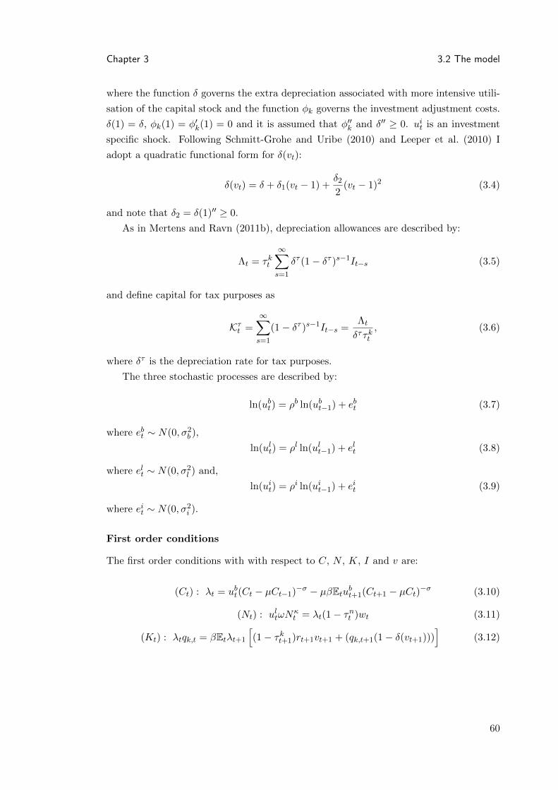
Chapter 3 3.2 The model
where the function δ governs the extra depreciation associated with more intensive utili-
sation of the capital stock and the function φk governs the investment adjustment costs.
δ(1) = δ, φk(1) = φ′k(1) = 0 and it is assumed that φ′′k and δ′′ ≥ 0. uit is an investment
specific shock. Following Schmitt-Grohe and Uribe (2010) and Leeper et al. (2010) I
adopt a quadratic functional form for δ(vt):
δ(vt) = δ + δ1(vt − 1) +δ2
2(vt − 1)2 (3.4)
and note that δ2 = δ(1)′′ ≥ 0.
As in Mertens and Ravn (2011b), depreciation allowances are described by:
Λt = τkt
∞∑s=1
δτ (1− δτ )s−1It−s (3.5)
and define capital for tax purposes as
Kτt =
∞∑s=1
(1− δτ )s−1It−s =Λt
δττkt, (3.6)
where δτ is the depreciation rate for tax purposes.
The three stochastic processes are described by:
ln(ubt) = ρb ln(ubt−1) + ebt (3.7)
where ebt ∼ N(0, σ2b ),
ln(ult) = ρl ln(ult−1) + elt (3.8)
where elt ∼ N(0, σ2l ) and,
ln(uit) = ρi ln(uit−1) + eit (3.9)
where eit ∼ N(0, σ2i ).
First order conditions
The first order conditions with with respect to C, N , K, I and v are:
(Ct) : λt = ubt(Ct − µCt−1)−σ − µβEtubt+1(Ct+1 − µCt)−σ (3.10)
(Nt) : ultωNκt = λt(1− τnt )wt (3.11)
(Kt) : λtqk,t = βEtλt+1
[(1− τkt+1)rt+1vt+1 + (qk,t+1(1− δ(vt+1)))
](3.12)
60

Chapter 3 3.2 The model
(It) : 1−qk,t(
1− φk(uitItIt−1
)− φ′k
(uitItIt−1
)uitItIt−1
)= βEt
λt+1
λt
(φ′k
(uit+1It+1
It
)uit+1I
2t+1
I2t
)+ Γt
(3.13)
where the term Γt is defined as
Γt = βδτEt[λt+1
λtτkt+1
]+ β(1− δτ )Et
[λt+1
λtΓt+1
], (3.14)
reflecting equation (3.5) which implies that the choice of investment today affects future
payments of depreciation allowances. Finally,
(vt) : (1− τkt )rkt = δ′(vt)qk,t. (3.15)
Equation (3.10) states that the marginal utility of consumption is equal to λt. Equa-
tion (3.11) sets the after-tax real wage equal to the marginal rate of substitution between
consumption and leisure. Equation (3.12) defines qt as the expected present value of
future rental rates less depreciation. Equations (3.13) and (3.14) describe the dynamics
of investment; the change in investment is related to the expected discounted present
value of current and future qt and Γt. Equation (3.15) determines the efficient level of
utilisation in terms of its current net return relative to the shadow value of the capital
stock.
3.2.2 Firms
The economy produces a single final good, in a perfectly competitive market, which is
used for consumption and investment by households. There are a continuum of interme-
diate goods producers, indexed by j ∈ [0, 1], who produce differentiated goods for use
in final production. There is monopolistic competition in the intermediate goods mar-
ket with each firm producing one differentiated good. This price-setting power allows
these firms to make pricing decisions, make steady state profit and face an exogenous
possibility of not being able to adjust their price as in Calvo (1983).
The final good is produced by combining intermediate goods
Yt =
∫ 1
0
[(yt(j))
ε−1ε dj
] εε−1
. (3.16)
Cost minimisation by final goods firms implies that demand for intermediate variety
yt(j) can be expressed as a function of its price relative to the aggregate price index and
aggregate output:
yt(j) =
(pt(j)
Pt
)−εYt, (3.17)
where pt(j) is the price of the intermediate good and Pt is the final consumer price index
61

Chapter 3 3.2 The model
(the price of the final good). Pt is defined as:
Pt =
∫ 1
0
[(pt(j))
1−εdj] 11−ε . (3.18)
ε is the price elasticity of demand faced by each monopolist.
Intermediate goods producers use technology
y(j) = Zt(vtKt−1(j))αNt(j)1−α (3.19)
where Zt is a productivity shock with ln(uzt ) = ρz ln(uzt−1) + ezt and ezt ∼ N(0, σ2z). Cost
minimisation implies that factor returns are paid their marginal product, distorted by a
markup:
vtrkt = αMCt
yt(j)
Kt−1(j)(3.20)
and
wt = (1− α)MCtyt(j)
Nt(j). (3.21)
As usual, it can be shown that marginal cost (MC) is common across producers and is
the inverse of the markup.7
The dynamics of price adjustment are governed by some firms being able to adjust
their price in a given period and some not. The ability to adjust price is governed by
a fixed probability as in Calvo (1983). Denote the probability that an intermediate
producer cannot adjust their price as η ∈ (0, 1). When firms are able to reset their price
they choose p∗t (j) to maximise expected profits
maxEt∞∑s=0
Qt,t+s[p∗t (j)Yt+s(j)−MCNt+syt+s(j)
], (3.22)
subject to
yt+s(j) =
(pt+s(j)
Pt+s
)−εYt+s,
where MCNt is nominal marginal cost.
The first order condition for firm j’s price setting problem is the familiar New Key-
nesian optimal reset price, common across all firms who reset in the same period:
p∗t (j) = P ∗t =ε
ε− 1
Et∑∞
s=0 ηsQt,t+sMCt+syt+s(j)
Et∑∞
s=0 ηsQt,t+syt+s(j)
. (3.23)
Finally, the price index is an aggregate of firms who reset their price today and those
who must retain last period’s prices
7See, for example, Gali (2008) or Smets and Wouters (2003).
62

Chapter 3 3.2 The model
Pt =[ηP
(1−ε)t−1 + (1− η)P
∗(1−ε)t
] 11−ε
. (3.24)
3.2.3 Monetary policy
The monetary authority follows a standard interest rate rule where the interest rate
responds to output, inflation and exhibits persistence
Rt = ψRRt−1 + (1− ψR)(ψππt + ψyyt) + eRt , (3.25)
where eRt is an i.i.d. interest rate shock: eRt ∼ N(0, σ2R). Variables with a hat represent
percentage deviations from steady state and πt = pt − pt−1 (with the model linearised
around a zero inflation steady state). The parameters are not restricted to satisfy the
Taylor principle. During estimation this allows the data to favour a model specification
with passive monetary policy and active fiscal policy (see Section 3.5).
3.2.4 Fiscal policy rules
Romer and Romer (2010) and Chapter 2 distinguish, in the narrative record, a variety
of motives given by policymakers for changing taxes. In this chapter I focus attention on
both ‘exogenous’ tax changes and the ‘endogenous’ categories which could be regarded as
responding to current or prospective conditions. In Chapter 2 I noted that the ‘exogenous’
deficit consolidation (which Romer and Romer (2010) simply call deficit-driven changes)
category could well be regarded as endogenous. One might argue: why cut the deficit at
all if it is not to forestall an adverse future shock? In this chapter I therefore combine
the deficit category in the Romer–Romer data with the other endogenous tax changes.
Hence, the ‘exogenous’ tax change category is net of deficit-motivated actions.8 This
means that the identified endogenous tax changes occurred in response to movements in
output, to fund spending decisions or to deal with the deficit and debt situation.
The model economy contains labour and capital tax rates. In solving and estimating
the model it will be linearised around a deterministic steady state (see Appendices B.1
and B.2). I therefore directly express the fiscal policy rules in linearised form. Define
the linearised ‘endogenous’ tax rate response (Υit for i = {nk}) as a function of output,
government spending and debt:
Υnt = γny yt + γnb bt−1 + γng gt + νnt (3.26)
Υkt = γky yt + γkb bt−1 + γkg gt + νkt . (3.27)
8Note that Romer and Romer (2010) and Chapter 2 show that excluding the deficit changes from theexogenous category does not affect the main results regarding the effect of tax changes on the macroe-conomy.
63

Chapter 3 3.2 The model
The νt terms are distributed νnt ∼ N(0, σ2N,n) and νkt ∼ N(0, σ2
N,k). These error terms
pick up expectational errors associated with policy actions that deviate from the expected
policy rule (the part captured by the γ terms). Note that these are not the same as the
‘exogenous’ shocks identified in the narrative approach. Furthermore, assume that the
linearised ‘exogenous’ tax rates, as measured by the narrative approach, can be captured
by autoregressive processes:
xnt = ρX,nxnt−1 + eX,nt (3.28)
xkt = ρX,kxkt−1 + eX,kt . (3.29)
where eX,nt ∼ N(0, σ2X,n) and eX,kt ∼ N(0, σ2
X,k).
The model’s linearised aggregate labour and capital tax rates, τnt and τkt , are then a
combination of endogenous and exogenous components. In other words
τnt = Υnt + xnt (3.30)
and
τkt = Υkt + xkt . (3.31)
Note that it is τnt and τkt that appear above in the model itself.
Following Leeper et al. (2010) I allow spending and lump sum transfers to respond
to debt and output as follows:
gt = −γgy yt − γgb bt−1 + ugt (3.32)
with
ugt = ρgugt−1 + egt (3.33)
and egt ∼ N(0, σ2g) and
LSt = −γLSy yt − γLSb bt−1 + uLSt (3.34)
with
uLSt = ρLS uLSt−1 + eLSt (3.35)
and eLSt ∼ N(0, σ2LS).
In addition, fiscal policies must satisfy the government budget constraint each period,
which is given by
Bt = rt−1Bt−1 +Gt + LSt − wtNtτnt − rkt vtKt−1τ
kt + Λt (3.36)
where rt−1 is the real interest rate at the end of period t − 1. Note that the Fisher
relationship implies rt = Rt − Etπt+1 (which can be obtained from the linearised first
64

Chapter 3 3.2 The model
order conditions). Total net tax revenue is given by
RTt = wtNtτnt + rkt vtKt−1τ
kt − Λt. (3.37)
3.2.5 Incorporating the narrative measures
The Romer–Romer narrative dataset was constructed using the prospective effect on rev-
enues. To relate the narrative shocks to the model, I first consider the revenue gained
from a particular narrative-identified shock. The total estimated revenue change identi-
fied by the narrative approach is a combination of the changes in the different tax rates.
Keeping with the above notation, define the implied ‘endogenous’ capital and labour tax
rates as Υit where i = {n, k} and the equivalent ‘exogenous’ tax rates by Xi
t . Total (net)
revenue from ‘endogenous’ tax rates, RN , can be thought of as
RNt = wt−1Nt−1Υnt + (rkt−1u
kt−1Kt−2 − δτKt−2)Υk
t (3.38)
and similarly for ‘exogenous’ taxes
RXt = wt−1Nt−1Xnt + (rkt−1u
kt−1Kt−2 − δτKt−2)Xk
t . (3.39)
Obviously these equations closely reflect the structure of the aggregate revenue equation
(3.37) and note that I have made use of equation (3.6). The lagged variables reflect that
the narrative shocks are measured ceteris paribus, although in practice this distinction
made little difference to the estimation results in the following sections.
The narrative measures themselves are the expected percentage point change in rev-
enues to GDP. I therefore divide equations (3.38) and (3.39) by period t GDP. These
equations are also linearised around the model’s deterministic steady state in keeping
with the rest of the model. Let εXt and εNt represent the model’s equivalent ‘exogenous’
and ‘endogenous’ narrative shocks. These are related to the corresponding linearised,
first-differenced, versions of (3.38) and (3.39) via a scaling factor reflecting the steady
state share of revenue generated by endogenous or exogenous tax actions in GDP. With-
out any empirical basis for calibrating this scaling factor it will be estimated. I will
denote the endogenous and exogenous scaling factors θN and θX respectively. Appendix
B.1 contains details on the linearised system and illustrates how the terms εXt and εNt
precisely relate to the linearised equivalents of equations (3.38) and (3.39).
3.2.6 Equilibrium and model solution
An equilibrium is an allocation {Yt, Ct, It,Kt−1, Nt, Bt−1, vt,Kt−1,Γt} and a price system
such that the allocation solves: the household’s problem, satisfying first order conditions
(3.10), (3.11), (3.12), (3.13), (3.14) and (3.15), the firm’s problem, satisfying conditions
(3.20), (3.21), (3.23) and (3.24), a set of fiscal policies {τnt , τkt , Gt, LSt} such that the
65

Chapter 3 3.3 Estimation
government’s budget constraint is satisfied, a monetary policy rule, a set of exogenous
processes and equilibrium conditions such that all markets clear with the aggregate re-
source constraint Yt = Ct + It +Gt satisfied.
The model is linearised around a deterministic steady state. The details of the lin-
earised model and the steady state relationships are presented in Appendices B.1 and
B.2 respectively. The collection of first order and equilibrium conditions can, in general,
be written as:
Et{f(st+1, st, st−1, ξt) = 0} (3.40)
where s is a vector of the model’s variables in percentage deviations from steady state
and ξ the vector of shocks. The solution to the DSGE model is of the form:
st = P (Θ)st−1 +Q(Θ)ξt (3.41)
where the coefficient matrices depend on the structural parameter vector Θ. In the next
section Θ will be estimated.
3.3 Estimation
I estimate the structural parameters of the model economy using likelihood-based Bayesian
methods. The model is estimated for the United States to maintain comparability with
other recent structural empirical work on fiscal policy. I use quarterly data from 1960Q1
to 2007Q4.9 The vector of observable time series contains consumption, investment,
government debt, government spending, hours worked, labour tax revenues, capital tax
revenues, the Federal Funds rate, inflation and the Romer–Romer measured exogenous
and endogenous shocks. Variables are detrended with a constant and linear trend.10
Consumption, investment, government spending, hours and revenues are all in logs and
are real per capita. Appendix B.3 explains the data construction in more detail.
The model contains structural shocks to productivity, government spending, invest-
ment productivity, labour supply, transfers, the Federal Funds rate and four shocks to
taxes. As discussed, the two shocks to the endogenous components can be interpreted
as expectational errors associated with actions deviating from the endogenous tax policy
rule. The two further exogenous, autoregressive, processes are related to the ‘exogenous’
policy shocks identified by Romer and Romer.
Mertens and Ravn (2011a) argue that the Romer–Romer shocks are likely to be
measured with error and estimate the degree of the measurement error using a SVAR
approach. Bayesian estimation lends itself naturally to including measurement equations
9This maintains comparability with the rest of the literature. It also therefore excludes the KoreanWar which is the only major episode in the Romer–Romer narrative where tax increases exactly matchedthe spending rise. Furthermore, Perotti (2007) shows that inclusion of the Korean War disproportionablydrives results in narrative approaches to identifying spending shocks.
10The non-zero elements of the Romer–Romer shocks are demeaned as in Mertens and Ravn (2011a).
66

Chapter 3 3.3 Estimation
for the Romer–Romer shocks, potentially providing an alternative route to estimating the
degree of noise in the narrative measures. Furthermore, without some measurement error
it would not be sensible to jointly include the Romer–Romer shocks and tax revenues in
the estimation. The measurement equations are:
RRNt = εNt + eNt (3.42)
and
RRXt = εXt + eXt (3.43)
where RRjt for j = {N,X} represent the observed Romer–Romer endogenous and exoge-
nous shocks and εXt and εNt were defined earlier.
However, in the formulation so far, the νt and xt shocks in equations (3.26), (3.27),
(3.30) and (3.31) would not be separately identified. Using a latent variable model,
Mertens and Ravn (2011a) estimate that the correlation between the Romer–Romer
‘exogenous’ narrative measure and the true variable is about 83 per cent. I therefore
calibrate the standard error of eXt so that the correlation between εXt and RRXt , when the
model is simulated at the posterior means, is 83 per cent. I also restrict the endogenous
and exogenous revenue to GDP ratios (the scaling factors θN and θX) so that they do
not jointly exceed the aggregate steady state revenue to GDP ratio.
The vector of observables is related to the model’s variables via a measurement equa-
tion
s∗t = H(Θ)st + ζt (3.44)
where ζt are the measurement errors and s∗t is the vector of observables mentioned above.
The model can therefore be set up as a system of measurement and transition equations.
The goal is to estimate the joint posterior distribution of the structural parameters Θ.
The log-likelihood is derived using the Kalman filter and the Sims algorithm csminwel is
employed to maximise the log posterior kernel with respect to the parameter vector Θ.11
The log posterior kernel is a combination of the likelihood of the data combined with
the priors which I will discuss in the next section. Having found the posterior mode, the
Metropolis-Hastings (MH) algorithm is used to sample from the posterior distribution
and construct the posterior distribution of the structural parameters in Θ. The MH
algorithm starts by constructing a Gaussian approximation around the posterior mode
(found using the csminwel algorithm) with a scaled covariance matrix. New candidate
parameter values are drawn from this constructed distribution and the algorithm must
decide whether to accept or reject draws which lower the value of the posterior kernel. It
is useful not to reject all such draws, accepting a seemingly inferior candidate may allow
the algorithm to leave a local maximum to reach a global one. The choice of the scaling
parameter is important as it governs the acceptance rate. I choose the scaling parameter
11All these algorithms are implemented using the Dynare Toolbox for Matlab.
67

Chapter 3 3.3 Estimation
Table 3.1: Calibrated parameters
Parameter Calibration
β 0.99α 0.3δ 0.025δτ 0.05τn 0.192τk 0.216GY 0.0772BY 0.293
to ensure acceptance rates close to 25 per cent. 2 million draws were generated with the
first 600,000 used as a burn-in period. I run four parallel Monte Carlo Markov Chains
and, on completion, diagnostics are performed to ensure convergence.12
3.3.1 Calibration and priors
Table (3.1) presents the calibrated parameter values for steady state variables and deep
parameters that will not be estimated. I calibrate the discount factor β = 0.99 which
implies an annual steady state interest rate of 4 per cent. The share of capital in output is
calibrated to be α = 0.3. The quarterly depreciation rate is equal to 0.025. The value of
utilisation, v, is assumed to be one in steady state. The tax rates, the ratio of government
spending to GDP and the ratio of debt-to-GDP are calibrated using the mean values from
the data (see Appendix B.3). These parameter choices are common in the literature. I
also calibrate the steady state depreciation for tax purposes to be twice the economic rate
of depreciation following Mertens and Ravn (2011b) and Auerbach (1989). As mentioned
above, the variance of the measurement error in the Romer–Romer exogenous shocks is
calibrated to deliver a correlation between the observed measure and the true shock
of 83 per cent. Tables (3.2) and (3.3) (presented later with the results) give the prior
distributions assigned to the other parameters in the model. The prior distributions for
the coefficient of risk aversion σ, the inverse of the Frisch elasticity κ, the strength of
consumer habits µ, the parameter governing investment adjustment costs φ′′k, the degree
of capital utilisation δ2, the price elasticity ε, the coefficients in the interest rate rule
ψR, ψπ and ψy, and the probability of firms facing a fixed price η are common in the
literature; for comparable prior assumptions see Smets and Wouters (2007) and Leeper
et al. (2010) among others. The density functions are chosen to reflect the restrictions on
parameters. σ, κ, φ′′k, δ2 are all greater than zero, so I assume a Gamma density. µ and
η lie between zero and one so I assume a Beta density. I also make the same assumption
for the persistence parameters in the stationary stochastic processes (the ρ terms). Note
that the assumption on the distribution of ψπ does not force the parameter to obey the
12These include univariate and multivariate convergence diagnostics and trace plots.
68

Chapter 3 3.3 Estimation
Taylor principle.
Commonly accepted ranges for the fiscal policy parameters are less common. Conse-
quently diffuse priors were chosen for the feedback from debt and output to the tax rates.
The coefficients γky and γny govern the elasticity of revenues to output. This elasticity
has attracted considerable attention as it plays an important role in the SVAR identifi-
cation scheme of Blanchard and Perotti (2002). Blanchard and Perotti (2002) calibrate
this elasticity, on the basis of externally constructed elasticities, at 2.08 per cent; a one
per cent increase in output leads to a 2.08 per cent increase in tax revenue. Mertens
and Ravn (2011a) show that the narrative shocks imply a higher elasticity, even after
accounting for measurement error. They find an estimate of around 3. These numbers
suggest that the γy coefficients should be at least between one and two. However, there
is considerable disagreement about this parameter, not least that the Blanchard–Perotti
assumption is based on a constructed elasticity which itself could be subject to concerns
regarding endogeneity. I therefore assume a uniform prior for the γy coefficients between
0 and 4, which implies a prior mean at 2 — marrying up with the estimate in Mertens
and Ravn (2011a).
I follow Leeper et al. (2010) and assume prior means of 0.4 for the debt feedback
coefficients γkb , γnb , γLSb and γgb but with a standard deviation of 0.2, which is quite
diffuse, particularly allowing for parameters close to zero. In Chapter 4 I will estimate
that the feedback from government spending to taxes appears low, I therefore assume a
prior mean of a similar magnitude at 0.1 and with a standard deviation of 0.05.
Finally, the standard errors for the i.i.d shocks are assumed to follow an Inverse
Gamma distribution with a prior mean of 1 and standard deviation of 4, making for very
diffuse priors.
G denotes that the prior distribution is assumed to be the Gamma distribution, Brefers to the Beta distribution, N to the Gaussian distribution, IG to the Inverse Gamma
distribution and U to a uniform distribution.
3.3.2 Estimation results
Tables (3.2) and (3.3) also report the means and 5% and 95% of the posterior distribution.
Figures (3.1) and (3.2) illustrate the prior distributions for the parameters together with
their estimated posterior distributions.
First I examine the estimates of the more standard parameters. The estimate of σ,
the degree of risk aversion, is well within the range of common estimates. For example,
the value in table (3.2) is between the posterior mean of 1.38 estimated by Smets and
Wouters (2007) and 2.7 estimated by Leeper et al. (2010) and Traum and Yang (2010).
The estimate of κ is also very similar to values in those papers. The strength of habit
persistence is slightly lower than usually estimated, with a posterior mean of around 0.4.
This is lower than the posterior mean of 0.7 estimated by Smets and Wouters (2007)
69

Chapter 3 3.3 Estimation
Table 3.2: Priors and baseline model posterior distribution
Parameter Prior Density Mean S.d. Posterior mean 5% 95%
σ G 1.75 0.5 2.2 1.5 2.9κ G 2 0.5 1.9 1.3 2.4µ B 0.5 0.2 0.41 0.33 0.50φk G 5 0.25 5.2 4.7 5.6δ2 G 0.7 0.5 0.0084 0.0024 0.014ε G 6 0.25 5.7 5.3 6.1
γky U 2 [0, 4] 1.9 1.2 2.6
γny U 2 [0, 4] 0.51 0.16 0.86
γgy G 0.07 0.05 0.063 0.0025 0.12γLSy G 0.2 0.1 0.19 0.056 0.34
γkb G 0.4 0.2 0.35 0.21 0.48γnb G 0.4 0.2 0.063 0.019 0.11γgb G 0.4 0.2 0.12 0.037 0.21γLSb G 0.4 0.2 0.23 0.077 0.38γng N 0.1 0.05 0.048 -0.018 0.011
γkg N 0.1 0.05 -0.0053 -0.081 0.069
θN G 0.07 0.025 0.061 0.053 0.068
ψπ N 1.5 0.25 1.7 1.51 1.84ψy N 0.125 0.05 -0.0033 -0.022 0.016ψR B 0.7 0.2 0.62 0.56 0.67η B 0.5 0.1 0.56 0.52 0.60
Table 3.3: The shocks: priors and baseline model posterior distribution
Parameter Prior Density Mean S.d. Posterior mean 5% 95%
ρz B 0.7 0.2 0.98 0.96 0.99ρg B 0.7 0.2 0.97 0.95 0.99ρi B 0.7 0.2 0.42 0.32 0.52ρb B 0.7 0.2 0.88 0.83 0.92ρl B 0.7 0.2 0.998 0.995 0.999ρLS B 0.7 0.2 0.97 0.95 0.99ρX,n B 0.7 0.2 0.97 0.94 0.99ρX,k B 0.7 0.2 0.95 0.92 0.98
σz IG 1 4 0.58 0.52 0.63σg IG 1 4 3.1 2.8 3.3σi IG 1 4 4.2 3.8 4.6σb IG 1 4 1.4 1.1 1.6σl IG 1 4 2.5 2.0 3.0σLS IG 1 4 6.0 5.4 6.5σX,n IG 1 4 2.3 2.0 2.5σX,k IG 1 4 3.7 3.2 4.1σR IG 1 4 0.33 0.29 0.37σN,n IG 1 4 2.2 1.9 2.5σN,k IG 1 4 1.1 0.50 1.6σN IG 1 4 0.25 0.23 0.27
70

Chapter 3 3.3 Estimation
0 2 4 60
0.5
1
Sigma
0 2 40
0.5
1
Kappa
0 0.2 0.4 0.6 0.80
2
4
6
8Mu
0 0.1 0.20
50
100
Delta2
4 5 6 70
0.5
1
1.5
Epsilon
1 1.5 2 2.50
2
4
Psi Pi
−0.1 0 0.1 0.20
10
20
30
Psi y
0.2 0.4 0.6 0.80
5
10
Psi R
0.3 0.4 0.5 0.6 0.70
5
10
15
Eta
Figure 3.1: Prior (grey, dashed) and posterior distributions (red, solid) of selected pa-rameters
71

Chapter 3 3.3 Estimation
0 0.5 10
2
4
6
8
Gamma gb
0 0.5 10
2
4
Gamma kb
0 0.5 10
5
10
15
Gamma nb
0 0.5 10
2
4
Gamma zb
0 2 40
0.5
1
Gamma ky
0 1 2 30
1
2
Gamma ny
0.05 0.1 0.150
20
40
60
80
Theta N
−0.2 0 0.20
2
4
6
8
Gamma kg
−0.2 0 0.20
5
10
Gamma ng
Figure 3.2: Prior (grey, dashed) and posterior distributions (red, solid) of selected coef-ficients from the fiscal policy rules
72
Chapter 3 3.3 Estimation
but within the 5% and 95% points of the posterior distribution found by Leeper et al.
(2010). The estimate of φ′′k is very similar to that obtained by Leeper et al. (2010)
but the estimate of δ2 is considerably lower. However, Schmitt-Grohe and Uribe (2010)
estimate the parameter δ2/δ1, with both the Bayesian posterior mean and the mean from
standard Maximum Likelihood estimation between 0.3 and 0.45. Mertens and Ravn
(2011b) also obtain a value for δ2/δ1 of around 0.6. Given that the steady state of the
model implies a δ1 of around 0.035, my estimate of δ2 implies a value for δ2/δ1 of 0.25,
within the confidence intervals estimated by Schmitt-Grohe and Uribe (2010). Traum
and Yang (2010) estimate a parameter which would imply a δ2 of about 0.02. Whilst my
estimate is slightly on the low side, it is not wildly different from other estimates in the
literature. The estimate of ε implies a steady state markup of 21%, which is similar to
values normally chosen for the calibration of New Keynesian models — see for example
Gali (2008).
The estimated parameters of the interest rate rule are also relatively standard. The
persistence in the Federal Fund rate is estimated to be around 0.6, which is similar to
the estimate by Zubairy (2010) of 0.52. The response of the interest rate to inflation
satisfies the Taylor principle, making monetary policy active. My estimate of 1.68 for the
posterior mean is slightly lower than the value of 2 found by Smets and Wouters (2007)
or 1.9 by Traum and Yang (2010). It is, however, slightly higher than the posterior mean
of 1.55 estimated by Zubairy (2010). The response of the Federal Funds rate to output
is interesting as it is not significantly different from zero. This is in contrast to estimates
in Smets and Wouters (2007) and Zubairy (2010), although their posterior estimates are
still low. My estimate of the posterior mean of the degree of price stickiness, η, is also
lower than common estimates, which often places it more in the region of 0.6-0.75. For
example, Smets and Wouters (2007) estimates the posterior mean of this parameter to be
0.66, although my estimate is still within the 5th and 95th percentiles of their posterior
distribution.
I now turn to the parameters of particular interest in this chapter, those governing
the response of the fiscal policy instruments. It is useful to keep in mind two separate
comparisons. First, I am interested in comparing my results with those in the wider
literature. Second, I compare my results in the baseline model with a version that does
not use the Romer–Romer data in the estimation of the model.
The inclusion of the Romer–Romer shocks produces a much lower estimate for γgb .
In comparison with Leeper et al. (2010), their posterior mean of 0.23 is outside the
90% Bayesian confidence intervals of my posterior distribution.13 When I compare this
baseline model to a version that excludes the Romer–Romer shocks, I also find that
the result is lower. Estimating the model without the Romer–Romer data produces an
estimate for γgb of 0.17. These results suggest that the feedback from debt to government
13This is also true when the feedback from spending to taxes is excluded (as it is in Leeper et al. (2010)and Zubairy (2010)).
73
Chapter 3 3.4 The effect of tax and spending shocks
spending is considerably weaker than previously estimated.
The posterior means for the feedback from debt to the tax rates are similar to Leeper
et al. (2010), although the response of capital taxes to debt is weaker. Comparing the
coefficient estimates in table (3.2) with a version of the model excluding the Romer–
Romer data I find that, in the baseline case, the feedback from debt to both taxes is
lower. Without using the Romer–Romer data, the feedback from debt to capital and
labour taxes would have been 0.4 and 0.09 respectively.
The responses of the tax rates to output are estimated to be stronger than in Leeper
et al. (2010). The posterior mean estimates for the response of capital and labour taxes
are both higher, although labour tax rates respond much less than capital tax rates. Later
I will consider the effect of excluding depreciation allowances. It is worth mentioning
at this stage that the model without depreciation allowances produces an even higher
estimate for γky , well above the estimates in Leeper et al. (2010) and closer to 3. Mirroring
the results I will obtain in Chapter 4, the response of the tax rates to movements in
government expenditure is estimated to be small.
3.3.3 Measurement error in the narrative endogenous tax changes
Mertens and Ravn (2011a) estimate that the Romer–Romer exogenous shocks exhibit an
83% correlation with the true (latent) variable. I discussed above that I make use of this
information to help identify parts of the model. However, I did not restrict the correlation
between the Romer–Romer endogenous shocks and the true (model-equivalent) variable.
The posterior mean of the standard error of the measurement error in the endogenous
shocks is 0.25. When I simulate the model at the estimated posterior means I find
that this estimated degree of measurement error, together with all the other estimated
parameters in the model, imply a correlation between the Romer–Romer endogenous
shocks and the true (model-equivalent) variable of about 55%. It is interesting that this
value is lower than the estimated correlation for the exogenous shocks found by Mertens
and Ravn (2011a), suggesting a higher degree of noise in the narrative endogenous tax
changes.
3.4 The effect of tax and spending shocks
As noted, for example by Baxter and King (1993), standard macroeconomic models can
produce a range of theoretical predictions for the effects of fiscal shocks depending on
how they are financed. The estimated endogenous feedback mechanisms in the previous
section will therefore have important implications. Consequently, I pursue impulse re-
sponse analysis and examine the fiscal multipliers associated with structural shocks to
the fiscal policy instruments.
74

Chapter 3 3.4 The effect of tax and spending shocks
3.4.1 Impulse response analysis
In this section I consider the model’s predictions for output, consumption, investment
and hours worked in response to a one standard deviation structural shock to government
spending, the capital tax rate and the labour tax rate.
Figure (3.3) shows that a one standard deviation increase in government expenditure
leads to a rise in output of nearly 0.2 per cent on impact. Consumption and investment
also both fall, as is the usual prediction of standard macroeconomic models. This is partly
driven by the wealth effect on labour supply which leads households to work harder in
response to decreased lifetime wealth. It also causes households to consume and save less
as their after-tax lifetime income has fallen (causing both consumption and investment to
fall). That output still rises in the face of changes in distortionary taxation implies that
the wealth effect dominates any substitution effects. In Chapter 4 I explore this issue
in more detail. In the bottom panels of figure (3.3) it can be seen that spending shocks
appear more debt-financed. Note that the tax rate responses are percentage changes
from steady state so, for example, the capital tax rate response is 1.5 per cent higher
than steady state after 16 quarters. Given a steady state rate of around 20%, this implies
the capital tax rate only changes by about 0.3 percentage points.
Figure (3.4) illustrates the effect of an exogenous cut in capital taxes. A one standard
deviation cut leads to a rise in output on impact of about 0.06, increasing to nearly 0.1
per cent after four quarters. The effect on consumption is very similar, stimulated by
the cut in taxes. The investment increase is strong as might be expected from a cut in
taxes on capital. Hours worked fall by about 0.1 per cent on impact, rising towards zero
over time as the marginal product of labour rises with the increasing capital stock.
75

Chapter 3 3.4 The effect of tax and spending shocks
Output
Perc
en
t
5 10 15−0.1
0
0.1
0.2
0.3Consumption
Perc
en
t
5 10 15−0.2
−0.1
0
0.1
Investment
Perc
ent
5 10 15−0.5
0
0.5Hours worked
Perc
ent
5 10 15−0.1
0
0.1
0.2
Government Debt
Perc
ent
5 10 150
2
4
6Capital tax rate
Perc
ent
5 10 150
0.5
1
1.5
2
2.5
Labour tax rate
Perc
ent
5 10 150
0.2
0.4
0.6
0.8
1
Figure 3.3: Response to a one standard deviation increase in government spending. 95%
confidence intervals.
76

Chapter 3 3.4 The effect of tax and spending shocks
Output
Perc
ent
5 10 150
0.05
0.1
0.15
0.2Consumption
Perc
ent
5 10 150
0.05
0.1
0.15
0.2
Investment
Perc
ent
Quarters5 10 15
0
0.1
0.2
0.3
0.4
0.5
Hours worked
Perc
ent
Quarters5 10 15
−0.15
−0.1
−0.05
0
0.05
Figure 3.4: Response to a one standard deviation cut in the exogenous capital tax rate.
95% confidence intervals.
Figure (3.5) illustrates the effect of a one standard deviation structural labour tax
rate cut. The plotted response of output and consumption is similar to a capital tax
cut. A one standard deviation cut leads to a 0.07 percent rise in output, peaking around
0.1 after four quarters. Investment also rises as consumers save some of the tax cut.
However, the implied investment multiplier is not as strong as with a capital tax cut,
which is to be expected. In the case of a capital tax cut, households are incentivised to
accumulate capital at the expense of consumption. In the next section I will examine the
multipliers themselves and show that the capital tax cut is much more expansionary than
the labour tax cut. Finally, figure (3.5) shows that, contrary to the capital tax cut, the
cut in taxes on labour generates a rise in labour supply by raising the after-tax return
to work.
77
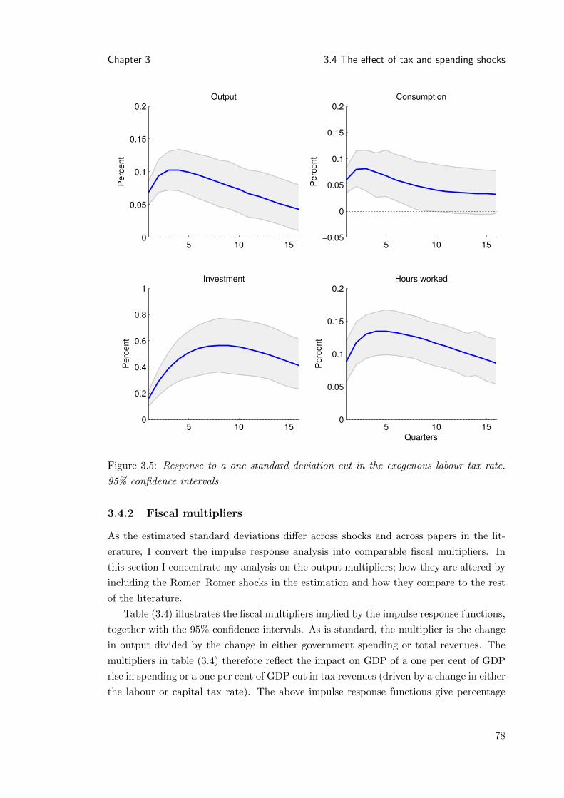
Chapter 3 3.4 The effect of tax and spending shocks
Output
Perc
ent
5 10 150
0.05
0.1
0.15
0.2Consumption
Perc
ent
5 10 15−0.05
0
0.05
0.1
0.15
0.2
Investment
Perc
ent
5 10 150
0.2
0.4
0.6
0.8
1Hours worked
Perc
ent
Quarters5 10 15
0
0.05
0.1
0.15
0.2
Figure 3.5: Response to a one standard deviation cut in the exogenous labour tax rate.
95% confidence intervals.
3.4.2 Fiscal multipliers
As the estimated standard deviations differ across shocks and across papers in the lit-
erature, I convert the impulse response analysis into comparable fiscal multipliers. In
this section I concentrate my analysis on the output multipliers; how they are altered by
including the Romer–Romer shocks in the estimation and how they compare to the rest
of the literature.
Table (3.4) illustrates the fiscal multipliers implied by the impulse response functions,
together with the 95% confidence intervals. As is standard, the multiplier is the change
in output divided by the change in either government spending or total revenues. The
multipliers in table (3.4) therefore reflect the impact on GDP of a one per cent of GDP
rise in spending or a one per cent of GDP cut in tax revenues (driven by a change in either
the labour or capital tax rate). The above impulse response functions give percentage
78

Chapter 3 3.4 The effect of tax and spending shocks
Table 3.4: Implied fiscal multipliers
Variable Impact Q4
∆Y∆Tn
0.27 0.41(0.22,0.31) (0.32,0.48)
∆Y∆Tk
0.73 1.12(0.65,0.78) (0.98,1.20)
∆Y∆G
0.77 0.45(0.75,0.79) (0.33,0.55)
Q4 is the peak for the tax multipliers; for government spending the peak is on impact.
deviations from steady state. The multiplier can therefore be computed making use of
the steady state values as follows
∆Yt+k∆Gt
=∆yt+k∆gt
Y
G(3.45)
with similarly defined multipliers for a one per cent cut in taxes as a proportion of GDP.
The multiplier for government spending is very close to that found by Leeper et al.
(2010) but lower than the impact effect of 1.12 estimated by Zubairy (2010). The govern-
ment spending multiplier is also very similar when the model in this paper is estimated
with and without using the Romer–Romer data.
The labour tax multiplier is considerably stronger than estimated by Zubairy (2010)
who finds an impact response of 0.13. My impact estimate is similar to that found by
Leeper et al. (2010); however the peak response shown in table (3.4) is much higher.
This is because the response in Leeper et al. (2010) peaks on impact, whereas I find the
effect builds over the first year. Again, the inclusion of narrative data in estimation of
my model does not affect the peak of the response.
The capital tax multiplier, however, is significantly higher once the Romer–Romer
shocks have been included. The impact response would have been estimated at around
0.6, peaking at around 0.9. The estimate in table (3.4) is also considerably higher than
the results of Leeper et al. (2010) and Zubairy (2010), the latter estimating an effect of
0.33 on impact and 0.36 at its peak. Making use of the Romer–Romer shocks therefore
has important implications.
In summary, the inclusion of the Romer–Romer shocks appears to increase the esti-
mated capital tax multiplier. The model in this chapter also produces higher estimates
of the effect of a labour tax cut than is found by Leeper et al. (2010). However, this is
true with and without the Romer–Romer shocks included in the estimation. The effect
of a shock to government expenditure is also similar with and without the Romer–Romer
shocks, similar to the results in Leeper et al. (2010) but smaller than the effect found by
Zubairy (2010).
79

Chapter 3 3.4 The effect of tax and spending shocks
3.4.3 A comparison with Romer–Romer
Continuing the discussion of fiscal multipliers, it is interesting to compare the estimated
effect of a cut in ‘exogenous’ taxes to the theory-free econometric approach in Romer and
Romer (2010). As discussed, the model contains narrative tax variables (model-equivalent
variables which are then related to the narrative measures). The model therefore produces
impulse response functions for the implied change in the narrative ‘exogenous’ taxes
following structural shocks. In this subsection I normalise the structural shocks to labour
and capital taxes to generate a one per cent fall in the model’s ‘exogenous’ narrative
variable. As such, this exercise simulates the results in Romer and Romer (2010). Given
that the narrative shocks are a combination of labour and capital tax changes there is
no good way, from the aggregate data, to choose the split between capital and labour
taxes. I therefore consider the two cases separately. It is worth keeping in mind that
the aggregate effect in Romer and Romer (2010) is likely to be some combination of the
results below, but it is still interesting to examine whether the magnitudes are similar.
Figure (3.6) illustrates the effect on output of a cut in the capital tax rate or the
labour tax rate, normalised such that the overall effect on the model’s narrative variable
εX is a one percentage point cut. There is a much larger effect of capital taxes than
labour taxes — reflecting the multipliers above. Figure (3.7) combines these results with
the VAR evidence obtained using the Romer–Romer data in the VAR specification in
Chapter 2.14
The capital tax shock is initially too expansionary relative to the aggregate Romer–
Romer result and lacks the hump-shaped build-up over time. The response to a labour
tax shock is more akin to the Romer–Romer results on impact but the overall profile
is too shallow. Some combination of the two tax shocks may well produce a response
somewhere in-between, although it appears the overall magnitude after quarter 10 will
still be lower.
There is an ongoing debate in the literature about the strength of the Romer–Romer
response due to it being much greater than SVAR estimates (see for example Favero
and Giavazzi (2010), Perotti (2010) and Mertens and Ravn (2011a)). Importantly, the
model estimated in this chapter also produces impact multipliers larger than comparable
SVAR estimates. In the SVAR literature the impact response is usually small, building
to between 0.5 and 1 per cent over time (see, for example, Perotti (2005)). The estimated
peak effect above, for both types of taxes, is also greater than the SVAR results in Perotti
(2005). It is interesting that the estimated model produces peak estimates somewhere in
between the SVAR results and the Romer–Romer results, even if the persistence is too
low.
14This replicates results very similar to those found in their original paper.
80

Chapter 3 3.5 Model comparisons and robustness
Capital tax shock: output response
Pe
rce
nt
2 4 6 8 10 12 14 160
0.5
1
1.5
2
2.5
3Labour tax shock: output response
Pe
rce
nt
2 4 6 8 10 12 14 160
0.5
1
1.5
2
2.5
3
Figure 3.6: Response of output to a one percentage point fall in the narrative exogenous
tax variable
Capital tax shock: output response
Perc
ent
2 4 6 8 10 12 14 160
0.5
1
1.5
2
2.5
3
3.5
4Labour tax shock: output response
Perc
ent
2 4 6 8 10 12 14 160
0.5
1
1.5
2
2.5
3
3.5
4
Figure 3.7: Output response implied the model (blue/dotted) and the Romer–Romer re-
sults (red/grey)
3.5 Model comparisons and robustness
3.5.1 Depreciation allowances and sticky prices
In this subsection I evaluate three versions of the baseline model. I examine how the
parameter estimates would differ when depreciation allowances and sticky prices are
excluded from the model. This facilities a closer comparison with Leeper et al. (2010)
and Zubairy (2010) whose models do not include these features.
81

Chapter 3 3.5 Model comparisons and robustness
Table (3.5) presents the parameter estimates from different versions of the baseline
model. First consider the model without depreciation allowances. The major difference
in the parameter estimates is a much higher value for γky , otherwise the results are similar.
I also report the log data density, estimated using the modified harmonic mean estimator
proposed by Geweke (1999). The model performs worse in terms of its log data density,
suggesting that the data favour the model with depreciation allowances included.
The flexible price model generates parameter estimates for σ and κ that are somewhat
higher than the sticky price model. The posterior mean for σ is the same as estimated by
Leeper et al. (2010). In terms of the fiscal policy coefficients, the feedback from output
to labour taxes is slightly higher, as is the feedback from debt to capital taxes. However,
the flexible price model also performs worse in terms of its log data density, therefore
favouring the baseline model.
3.5.2 Exogenous or endogenous fiscal policy?
As discussed by Leeper (1991), Benhabib et al. (2001) and Woodford (2003), among oth-
ers, there are potentially important interactions between the stance of monetary and fiscal
policy. These papers have shown that when fiscal policy endogenously reacts (strongly
enough) to debt, monetary policy must often satisfy the Taylor principle to ensure sta-
ble debt dynamics.15 The literature has referred to this case as one of ‘passive’ fiscal
policy and ‘active’ monetary policy. Alternatively, this fiscal stance is sometimes called
‘(locally) Ricardian’ following Woodford (2003). In the baseline model ψπ is estimated
to be greater than one (with ψy close to zero), thus satisfying the Taylor principle. The
coefficients determining the feedback to the fiscal policy instruments were all greater than
required to satisfy the condition for passive fiscal policy.16
However, if fiscal policy were entirely unresponsive — ‘active’ or ‘non-Ricardian’ —
monetary policy would need to be passive and violate the Taylor principle to ensure de-
terminate debt dynamics. Consider a simple example of a debt-financed tax cut adopted
from Davig and Leeper (2006). A debt-financed tax cut does not raise the present
value of future taxes (given exogenous processes for the fiscal instruments). Households
therefore perceive this as an increase in their lifetime wealth which, at initial prices
and interest rates, raises the demand for goods. Monetary policy must not react too
strongly (formally, it must violate the Taylor principle) because, as explained by Davig
and Leeper (2006), three channels then act to satisfy the government’s intertemporal
budget constraint (after imposing the transversality condition). First, passive monetary
policy allows the money stock to to expand and clear the market, creating seignorage
revenue. Second, surprise inflation revalues outstanding nominal debt. Third, lower real
interest rates allow a higher level of debt to be serviced for a given stream of primary
15See Benhabib et al. (2001) for conditions under which, given a Ricardian (or ‘passive’) fiscal policy,active monetary policy still does not ensure determinate equilibrium dynamics.
16That is, fiscal policy instruments respond enough to at least pay back the debt interest.
82

Chapter 3 3.5 Model comparisons and robustness
Table 3.5: Model comparisons
Parameter Baseline No D.A. Exogenous policy Flexible prices
σ2.2 2.2 1.1 2.7
(1.5,2.9) (1.5,2.9) (0.7,1.4) (2.0,3.4)
κ1.9 2.1 1.4 3.1
(1.3,2.4) (1.5,2.7) (0.9,1.9) (2.3,3.8)
µ0.4 0.4 0.6 0.14
(0.3,0.5) (0.3,0.5) (0.5,0.7) (0.04,0.2)
φ′′k5.2 5.2 5.1 5.1
(4.7,5.6) (4.8,5.6) (4.7,5.5) (4.7,5.5)
δ20.008 0.01 0.01 0.006
(0.002,0.01) (0.003,0.02) (0.004,0.02) (0.002,0.01)
ε5.7 5.6 5.7 5.7
(5.3,6.1) (5.1,6.0) (5.3,6.1) (5.3,6.1)
γky1.9 2.8 - 1.8
(1.2,2.6) (2.2,3.4) (1.0,2.6)
γny0.5 0.3 - 0.8
(0.2,0.9) (0,0.5) (0.4,1.2)
γgy0.06 0.06 - 0.07
(0.003,0.1) (0.003,0.1) (0.003,0.1)
γkb0.35 0.25 - 0.55
(0.21,0.48) (0.1,0.4) (0.41,0.68)
γnb0.06 0.07 - 0.03
(0.02,0.1) (0.02,0.1) (0.009,0.06)
γgb0.1 0.1 - 0.1
(0.04,0.2) (0.04,0.2) (0.03,0.17)
γng0.05 0.04 - 0.01
(-0.02,0.1) (-0.03,0.1) (-0.06,0.08)
γkg-0.005 0.01 - 0.01
(-0.08,0.07) (-0.06,0.08) (-0.07,0.08)
θN0.06 0.08 0.07 0.06
(0.05,0.07) (0.07,0.09) (0.06,0.09) (0.05,0.07)
ψπ1.7 1.7 0.999 1.8
(1.5,1.8) (1.5,1.9) (0.995,1.0) (1.6,2.0)
ψy-0.003 0.001 - -0.02
(-0.02,0.02) (-0.02,0.02) (-0.04,0.006)
ψR0.62 0.67 0.62 0.46
(0.56,0.67) (0.62,0.71) (0.57,0.68) (0.37,0.55)
η0.56 0.62 0.88 -
(0.52,0.60) (0.59,0.66) (0.86,0.90)
Log data density 0 -44 -69 -112(relative)
83

Chapter 3 3.6 Conclusion
surpluses. This active fiscal-passive monetary policy case is often referred to as the Fiscal
Theory of the Price Level.
To consider this possibility, column four of table (3.5) presents the results from a
model where fiscal instruments do not respond endogenously (equivalent to the case where
the γ terms are set to zero). Fiscal policy is therefore described by exogenous processes,
which are still related to the Romer–Romer shocks to make the model comparable. ψπ is
estimated to be less than one, which satisfies the condition for passive monetary policy
(although ψπ is not restricted to be less than one).
However, the results in table (3.5) imply that the model with fiscal feedback is pre-
ferred by the data in terms of the log data density. This suggests that, at least over
the whole sample, fiscal policy is sufficiently responsive to debt to ensure determinate
debt dynamics. This result is similar to findings by Traum and Yang (2010). These
authors also estimate a DSGE model using Bayesian methods and examine whether the
data prefer active monetary-passive fiscal policy or passive monetary-active fiscal policy.
They also find that the data prefer the active monetary-passive fiscal policy specification,
although their fiscal policy specification is not as rich as above.
The results presented here do not, of course, consider the possibility that there were
specific periods in the sample of passive or active fiscal policy. Recent work by, for
example, Davig and Leeper (2006, 2011) estimate regime-switching policy rules for the
United States, highlighting that different combinations of passive and active monetary
and fiscal policy existed at different points in the post-war period. The use of narrative
data presents an interesting avenue for future research in this direction.
3.6 Conclusion
In this chapter I have estimated a DSGE model using Bayesian methods to help under-
stand the importance of the endogenous feedback from key macroeconomic variables to
fiscal policy instruments. The central innovation in this chapter has been to make use
of new, direct measures of tax changes constructed using a ‘narrative’ approach. Other
methods, such as previously estimated DSGE models and SVARs, assume that the true
tax shocks are unobserved, attempting to identify these using structural assumptions and
performing estimation using National Accounts measures of tax revenues.
I showed how the narrative tax shocks can be integrated into a relatively stan-
dard medium-scale DSGE model. I then estimated the parameters in the model using
likelihood-based Bayesian techniques for the United States. The central results of this
paper are threefold. First I showed that, having made use of the narrative tax changes
identified by Romer and Romer (2010), the feedback from debt to the fiscal instruments
is reduced. My new estimates were also shown to be lower than comparable results by
Leeper et al. (2010). This was particularly true for the response of spending to debt and,
to a lesser extent, the response of capital taxes to debt.
84

Chapter 3 3.6 Conclusion
Second, I showed that the capital tax multiplier is significantly increased when the
Romer–Romer data are used in estimation of the model. Furthermore, in general, the
tax multipliers I obtain are higher than those estimated elsewhere in the literature. In
addition, I showed that the estimated model implies that exogenous tax changes have
a peak effect between estimates found by Romer and Romer (2010) and in the SVAR
literature. The effect of a government spending shock is found to be similar to the results
in Leeper et al. (2010) but lower than in Zubairy (2010). In Chapter 4 I consider the
transmission mechanisms of government spending shocks in more detail.
Third, I showed that the data prefer the baseline specification to three other versions
of the model. Versions of the model that exclude depreciation allowances and sticky
prices produced parameter estimates that were, in many cases, similar but there was
a deterioration in the estimated log data density. I also showed that the data appear
to prefer the model which allows for endogenous feedback to fiscal policy instruments.
An important corollary of this is that the fiscal instruments appear to react sufficiently
strongly to debt in the baseline model to ensure that passive monetary policy was not
needed to ensure stable debt dynamics. However, as discussed previously, work by Davig
and Leeper (2006, 2011) suggests the existence of different active/passive regimes at
different points in the post-war sample. Bringing narrative data to bear on these issues
is a potentially exciting avenue for further research.
Narrative data provide a rich new source of information for estimating the macroe-
conomic effects of fiscal policy. This chapter has shown that incorporating these new
measures into the estimation of a medium-scale DSGE model has important implications
for the estimated strength of feedback from debt and output to the fiscal instruments, as
well as the implied fiscal multipliers in response to structural fiscal policy shocks. Making
greater use of this new source of data provides interesting scope for future work.
85

Chapter 4
Government spending, wealth
effects and distortionary taxation
4.1 Introduction
The effectiveness of government spending in stimulating the economy became a central
policy question during the 2008 financial crisis. Whilst proponents and critics argued
about the mechanisms determining policy success, I noted in Chapter 3 that standard
macroeconomic models can generate a wide range of theoretical predictions depending
on the assumptions made about how the spending increase is financed1 and assumptions
about how consumers respond to implied future tax increases.
In Chapter 3 I pursued a full-information approach, estimating a DSGE model using
Bayesian methods. Although appealing as a method for identifying the endogenous
feedback from variables such as output or debt, full-information methods impose a lot of
structure on the data. As I discussed in Chapter 1, considerable faith must therefore be
placed in the model.
In recent years, a debate has emerged as to whether DSGE models can adequately
account for the empirical effects of structural shocks to government expenditure found
elsewhere in the empirical literature. For example, particular attention has been paid to
whether DSGE models can account for SVAR evidence that private consumption and real
wages tend to rise following a structural shock to government spending; see, for example,
Monacelli and Perotti (2009), Ravn et al. (2007) or Linnemann (2006).2
In this chapter I again construct and estimate a DSGE model for the United States.
However, rather than assuming the model is a full description of the data generating
process, I focus on the model’s ability to account for a particular aspect of the data:
namely the effect of government spending shocks. I employ a minimum distance ap-
1Also see, for example, Baxter and King (1993) or Alesina et al. (2002).2It should be noted that narrative identification approaches have tended to find a fall in private
consumption. For a review of this evidence and a reconciliation with the SVAR results see Perotti (2007).
86

Chapter 4 4.1 Introduction
proach, matching the impulse response functions from the model to those obtained from
a SVAR, identified using the method of Blanchard and Perotti (2002). Results from the
estimated model can then be compared with the SVAR evidence to evaluate the model’s
performance.
This chapter is particularly concerned with the endogenous response of tax rates to
government spending shocks and the strength of the so-called ‘wealth effect’ on labour
supply — both of which crucially affect the predictions of standard macroeconomic mod-
els. The estimated model is shown to match key aspects of the empirical evidence with
a realistic set of tax instruments and transmission channels.
For all their complexity, many standard models of fiscal policy often rely on a very
simple fiscal policy instrument, the lump sum tax, to finance an expenditure shock. This
includes state of the art policy models such as that of Smets and Wouters (2007) and
recent papers, for example by Cogan et al. (2010), who analyse the size of fiscal multipliers
in the U.S.
However, the lump sum tax assumption is far from innocuous. Lump sum tax-finance
implies a ‘wealth’ effect as (expected) income falls. Consumption falls but, assuming
leisure and consumption are normal goods, labour supply and consequently output rise.
This allows the neoclassical model, and others based on it, to match empirical evidence
that GDP increases following a discretionary government spending stimulus.
There are, however, several issues with this mechanism. Firstly, the output rise relies
both on the strength of the wealth effect and the lack of distortions associated with the
instrument. Consider using a labour income tax instead. The labour supply decision is
now distorted, producing strong negative substitution effects. Generally this substitution
effect dominates, lowering labour supply and output. Secondly, even if the wealth effect
channel can explain the output response, it generates consumption and the real wage
responses that are at odds with the empirical Structural Vector Autoregression (SVAR)
literature.3 Thirdly, there is the practical realism of the assumption. Lump sum taxes
are rarely, if ever, used as primary instruments of tax policy. Chapter 2 and Romer and
Romer (2010) illustrate that most tax actions in the U.K. and U.S. respectively were
changes in distortionary taxes.4
Since there is no a priori reason to assume that a particular mix of tax instruments
finances a spending increase, my first goal in this chapter is to estimate the endogenous
response of tax rates for the United States and construct a New Keynesian model which
replicates these.
The second goal is then to examine the strength of the wealth effect on labour supply
itself. The wealth effect channel is still potentially important even after modelling and
estimating the distortionary tax rules. This is because the government’s budget con-
3Again, see Perotti (2007) for a review of this evidence.4This includes, for example, both tax changes to directly fund spending measures and tax changes to
deal with a budget deficit.
87

Chapter 4 4.1 Introduction
straint must hold in each period. In several models (such as Burnside et al. (2004)), this
is done using a lump sum tax. Furthermore, even if the budget constraint is satisfied
by issuing debt, Ricardian equivalence with respect to lump sum taxes implies the same
wealth effect on labour supply. It is therefore important to consider jointly the strength
of the wealth effect on labour supply and the endogenous tax responses to the spending
shock.
Following Monacelli and Perotti (2009), I use Jaimovich and Rebelo (2009) (JR)
preferences which allow for a variable wealth effect on labour supply. Following Schmitt-
Grohe and Uribe (2010) (who do not investigate fiscal policy issues), I estimate the size
of this effect. As shown by Monacelli and Perotti, a useful feature of these preferences is
that, when the wealth effect on labour supply is limited, consumption and the real wage
can increase. This further motivates estimating the importance of the channel.
To evaluate the importance of other potential transmission mechanisms I include a
range of more standard features such as sticky prices, variable capital utilisation and
habits. I show that the estimated model can match the positive empirical response of
key variables including output, consumption and the real wage, which is a challenge
for many New Keynesian models. These results arise for a number of reasons. Firstly,
the importance of the wealth effect on labour supply is small. Secondly, mechanisms
such as sticky prices, variable capital utilisation, investment adjustment costs and habits
all play an important role in matching the evidence. Thirdly, distortionary tax rates
rise following the expenditure shock but their small magnitude crucially reduces the
distortions involved. This explains why the positive output and consumption responses
prevail.
The results in this chapter contribute, and are related, to several branches of the
current literature. Firstly, I directly contribute to the literature which seeks to explain
the empirical effects of discretionary shocks to government expenditure. As discussed
above, much work has been focused on matching the sign of the consumption (and real
wage) response.5 Few papers in this specific branch of the literature have considered
distortionary taxes or included empirically realistic tax policy rules (Burnside et al. (2004)
and Reis (2008) being two exceptions). To my knowledge, no papers have empirically
evaluated the importance of the wealth effect channel as a transmission mechanism of
fiscal policy.6
Secondly, by estimating tax policy rules, the results in this chapter have a relationship
with the literature discussed in Chapter 3, and to which Chapter 3 contributes. Both
Leeper et al. (2010) and Zubairy (2010) perform Bayesian estimation of DSGE models
that include feedback to the tax rates from output and debt (but not spending). However,
5Zubairy (2009), as I do, follows a minimum distance approach, estimating how well a ‘deep habits’model of the form of Ravn et al. (2007) (with lump sum taxes) can explain a government spending shock.
6Although, as noted above, Monacelli and Perotti (2009) do show how varying the strength of thiseffect has useful implications.
88

Chapter 4 4.2 The empirical effects of government spending shocks
Leeper et al. (2010) does not focus on the effects of spending shocks and Zubairy (2010)
is more concerned with estimating fiscal multipliers using a DSGE model rather than
matching other empirical evidence on the effects of spending shocks.
The remainder of the chapter is structured as follows. Section 4.2 estimates the
empirical effects of government spending shocks using a SVAR. Section 4.3 sets up the
theoretical model. Section 4.4 illustrates key features of the model with respect to the tax
policy rules and their interaction with the wealth effect channel. Section 4.5 estimates
the model using a minimum distance estimator. Section 4.6 concludes that the estimated
model matches the empirical evidence well, that shocks appear largely debt-financed,
that the wealth effect is relatively small and that sticky prices play an important role, as
do the other common mechanisms.
4.2 The empirical effects of government spending shocks
4.2.1 Identification
The parameters of the model will be chosen to match the estimated empirical impulse
response functions. The empirical effects of a government spending shock are identified
using the method of Blanchard and Perotti (2002). Consider the following reduced form
VAR:
Xt = α0 + α1t+B(L)Xt−1 + ut. (4.1)
X = [gt τk τn y c n w i b]′ where g is government spending, τk capital taxes, τn
labour taxes, y output, c consumption, n employment, w the real wage and i investment.
For later reference, I also include government debt, b. B(L) is a lag polynomial of order
P .
The reduced form residuals ut are likely to be correlated. For example, a shock to
government spending is likely to imply contemporaneous effects on taxes, debt and so
on. Pre-multiplying equation (4.1) by the square matrix A (and ignoring the constant
and trend for presentation) yields:
AXt = AB(L)Xt−1 + et (4.2)
where Aut = et and et are the structural shocks.7
7Sometimes this is written as Aut = Bet. I am therefore assuming B = I, which is common. It isworth noting that assumptions on A will replicate having some non-zero off-diagonal elements in B. SinceI only consider structural government spending shocks, all other elements of et will be 0 and only thefirst column of B is relevant. Suppose that the second element of this column was non-zero. This wouldimply that the structural government spending shock affects the tax (where tax is the second equation)reduced form residual. However, since ug = eg by the Blanchard–Perotti timing assumptions, nothing islost by setting this element of B to zero but ensuring that the relevant element of A, the effect of ug onother elements of ut, is correctly accounted for.
89

Chapter 4 4.2 The empirical effects of government spending shocks
Identification proceeds by making assumptions about the contemporaneous correla-
tion between variables. Identification is achieved by restricting n(n − 1)/2 parameters.
The Blanchard–Perotti assumptions justify certain restrictions. The key assumption is
that policy decision variables are unaffected contemporaneously (within the same quarter)
by changes in the other endogenous variables. This is justified by the institutional delays
involved in policy decision-making. It is therefore assumed that government spending is
not affected contemporaneously by any other variable.
The original Blanchard–Perotti approach, as discussed in Chapter 2, made use of
tax revenues as the measure of taxes, from which they had to work out how much of
the change in revenues was due to cyclical movements (in income, for example) and how
much was due to genuine policy shocks. External information on tax elasticities was used
to disentangle the two effects. In my empirical setup I follow Perotti (2007) and directly
construct, and use, tax rates so that the theoretical model’s policy rules can be directly
estimated. The consequence of using rates rather than revenues is that they are policy
decision variables. Under the Blanchard–Perotti timing assumptions, these should also
be unaffected by other endogenous variables within the quarter. However, I allow them
to be affected by spending (in other words, I assume that spending decisions are taken
first and then taxes can respond).
To illustrate the identification scheme, consider a smaller set of variables: govern-
ment spending g, a distortionary tax rate τ , a non-fiscal variable such as output or
consumption, y, and debt, b. The relationship between the reduced form residuals and
the structural shocks can be written as:1 −αgτ −αgy −αgb−ατg 1 −ατy −ατb−αyg −αyτ 1 −αyb−αbg −αbτ −αby 1
=
ugtuτt
uytubt
=
egteτt
eytebt
(4.3)
The timing assumptions discussed above allow us to set αgτ = αgy = αgb = ατy =
ατb = 0. However, it seems sensible to assume that taxes, output and debt may re-
spond to the structural spending shock. Output and debt may also respond to taxes
contemporaneously.
In the example above, these assumptions leave us one restriction short. We need to
restrict either αyb or αby. With the variable ordering above, setting αyb = 0 implies a
lower triangular matrix for A. Following Perotti (2007) I adopt this procedure. The
most contentious assumption is therefore that debt is ordered last. Ordering the debt
series last implies that debt has no contemporaneous effect on output within the quarter
(or that the level of debt in period t is the outcome of the changes to the other variables
and not the other way around). Ordering debt before output assumes that output has
no effect on debt (αby = 0) within the quarter. The latter assumption would appear
90

Chapter 4 4.2 The empirical effects of government spending shocks
unrealistic and so I opt for the former specification.8
4.2.2 The data
The data are for the United States over the period 1955:1 to 2007:4. I exclude the Korean
War because it is, to some extent, a unique event and can disproportionately drive the
results (see Perotti (2007)).
With the exception of the tax rates and debt, all data are taken directly from the
relevant sources (and appropriately deflated). The tax rates are constructed using the
method outlined in Jones (2002). This approach is also adopted by Burnside et al. (2004).
The debt series would ideally be ‘Debt Held by the Public’, as used by Favero and
Giavazzi (2007). However, this quarterly series does not go back far enough. I therefore
construct a debt series from old editions of the U.S. Treasury Bulletin. The resulting
series is very close to ‘Debt Held by the Public’, see Appendix C.1 for details. This
improves on the Favero–Giavazzi method of simulating the debt series back to 1947
using annual data.
All variables, except the tax rates, are the log of real per capita variables. The tax
rates are percentages. All real series are the nominal series deflated by its own implicit
price deflator, with the exception of government spending and debt which are deflated
by the GDP deflator. Appendix C.1 sets out the specific details of each series.
4.2.3 Results
The figures below report the baseline results for P = 4. The impulse response functions
are simulations to a one percent structural shock to government spending. The point
estimates are shown together with standard 68 percent non-parametric bootstrapped
confidence intervals using 10,000 replications.
Figure 4.1 shows the response of the fiscal policy variables to the shock. The response
of the labour and capital tax rates, although positive (as one might expect) are relatively
modest.9 Given the modest increase in taxes, it is useful to consider the response of
debt. To the extent that lump sum taxes are rarely used to satisfy the government
budget constraint, modest tax rate increases would imply a larger increase in debt. This
is what is observed in the fourth panel of figure (4.1).
Figure 4.2 shows the responses of the other variables in the SVAR. The top two panels
show the familiar SVAR result that output and consumption rise following a government
spending shock. The output response on impact is 0.224. Note that this is log yt − log y
8In the full specification I tested alternative variable orderings. Not placing debt last, despite the abovediscussion, generated identical impulse response functions to three decimal places, with the standarderrors only marginally affected. I switched the two tax rates around and this made little difference. Ialso used different combinations of the non-fiscal variables (which all appear in place of y in the shorterexample), again with very little effect.
9These responses are very similar including and excluding the debt series.
91

Chapter 4 4.2 The empirical effects of government spending shocks
and log gt−log g = 1 by definition. This means that the ratio of the percentage deviations
can be written as ∆yt∆gt
gy . The multiplier, ∆yt
∆gt(as in Chapter 3), is therefore the product
of this ratio and average government spending to GDP ( gy ), which is 0.22 in the sample.
These estimates imply an output multiplier of about one.
Government Spending
Perc
en
t
0 4 8 12 16−1
−0.5
0
0.5
1Capital Tax Rate
Perc
en
t0 4 8 12 16
−0.2
−0.1
0
0.1
0.2
Labour Tax Rate
Quarters
Perc
ent
0 4 8 12 16−0.2
−0.1
0
0.1
0.2Government Debt
Perc
ent
Quarters0 4 8 12 16
−1
−0.5
0
0.5
1
Figure 4.1: Impulse responses for the fiscal policy variables
92
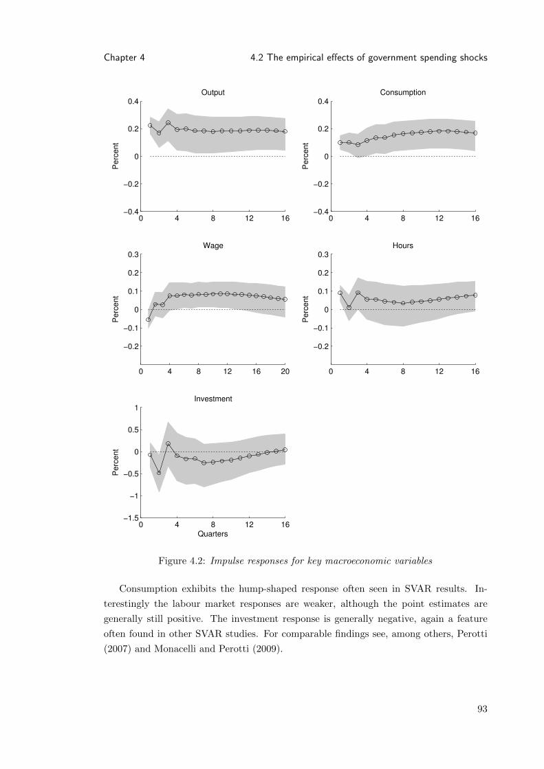
Chapter 4 4.2 The empirical effects of government spending shocks
Output
Pe
rce
nt
0 4 8 12 16−0.4
−0.2
0
0.2
0.4Consumption
Pe
rce
nt
0 4 8 12 16−0.4
−0.2
0
0.2
0.4
Wage
Pe
rcen
t
0 4 8 12 16 20
−0.2
−0.1
0
0.1
0.2
0.3Hours
Pe
rcen
t
0 4 8 12 16
−0.2
−0.1
0
0.1
0.2
0.3
Investment
Quarters
Pe
rce
nt
0 4 8 12 16−1.5
−1
−0.5
0
0.5
1
Figure 4.2: Impulse responses for key macroeconomic variables
Consumption exhibits the hump-shaped response often seen in SVAR results. In-
terestingly the labour market responses are weaker, although the point estimates are
generally still positive. The investment response is generally negative, again a feature
often found in other SVAR studies. For comparable findings see, among others, Perotti
(2007) and Monacelli and Perotti (2009).
93

Chapter 4 4.3 The model
4.3 The model
To directly address the issues raised earlier, the model includes distortionary capital and
labour tax rates, allowing for endogenous tax rate responses to government spending
shocks. I also employ Jaimovich and Rebelo (2009) preferences which allow the strength
of the wealth effect on labour supply to vary. Finally, the model includes a range of more
standard features such as sticky prices, variable capital utilisation and habits.
4.3.1 Households
Households derive utility from consumption (C) and leisure (1 − N). The household
maximises lifetime utility
maxCt,Nt,It,zt,Kt+1,Bt+1
Et∞∑t=s
βt−su(Ct+s, 1−Nt+s), (4.4)
subject to a budget constraint (in real terms)
Ct + It +Bt+1
Rt= Bt + wtNt(1− τNt ) + rKt (zt)(1− τKt )Kt − Tt + Πt. (4.5)
The capital stock evolves according to
Kt+1 = (1− δ(zt))Kt + It
(1− φ
(ItIt−1
− 1
)), (4.6)
which incorporates adjustment costs employed by Christiano et al. (2005), among others.
The utility function, u : R2 → R, is assumed to be concave and twice continuously
differentiable. The function φ satisfies φ = φ′ = 0 and φ′′ ≥ 0.
Kt+1 denotes capital held by households at the end of period t and Bt+1 are real
holdings of government bonds, also at the end of period t. Ct is consumption, It is
investment, Rt is the aggregate real interest rate (gross), wt is the aggregate real wage
and rKt is the real return on capital. τKt and τNt are the tax rates on capital and labour
income respectively. Tt are lump sum taxes. δ is the rate of depreciation. Πt are profits
distributed lump sum to households.
The parametric specification for the utility function u(·) follows Jaimovich and Rebelo
(2009), Schmitt-Grohe and Uribe (2010) and Monacelli and Perotti (2009).
U(Ct, Nt) =(Ct − hCt−1 − ψN ξ
tXt)1−σ
1− σ(4.7)
where
Xt = (Ct − hCt−1)γX1−γt−1 . (4.8)
For γ = 1 and h = 0 these preferences become those considered by King et al. (1988).
For γ = 0 and h = 0 they become the preferences considered by Greenwood et al. (1988)
94

Chapter 4 4.3 The model
(henceforth GHH).The latter preferences exhibit no wealth effect on labour supply. In
other words, labour supply is solely affected by the real wage (net of taxes) and not by
the level of consumption.10
I have modified the Jaimovich–Rebelo preferences to include habits. Ct−1 is aggregate
consumption in the previous period and the consumer takes this as given. Below I
show that internal habits, where consumers explicitly consider Ct−1 in their optimisation
decisions, would reintroduce the wealth effect on labour supply when γ = 0.
The model also features variable capital utilisation. High utilisation by firms implies
greater depreciation of a given stock of capital. For this reason both the return on capital
and the depreciation are functions of utilisation, captured by the variable zt.
First order conditions
The first order conditions for the household’s problem, with respect to Ct, Xt, Bt+1, Nt,
It, Kt+1 and zt are:
λt = (Ct − hCt−1 − ψN ξtXt)
−σ + µtβγ(Ct − hCt−1)γ−1X1−γt−1 (4.9)
(Ct − hCt−1 − ψN ξtXt)
−σψN ξt + µt = βEt(µt+1(1− γ)(Ct − hCt−1)γX−γt (4.10)
Et(λt+1
λt
)=
1
Rtβ(4.11)
ψN ξ−1t ξXt(Ct − hCt−1 − ψN ξ
tXt)−σ = λtwt(1− τnt ) (4.12)
1−qt(
1− φ(
ItIt−1
− 1
)− φ′
(ItIt−1
− 1
)(ItIt−1
))= Et
(qt+1
λt+1
λtβ
[I2t+1
I2t
φ′(It+1
It− 1
)]) (4.13)
qt = βEt[λt+1
λt
(rKt+1(1− τKt+1) + qt+1(1− δ(zt))
)](4.14)
(1− τKt )r′Kt (zt) = qtδ′(zt) (4.15)
where r′K is the derivative of the return on capital with respect to utilisation. µt is the
Lagrange multiplier on the evolution of Xt (equation (4.8)) and qt is the multiplier on
the capital accumulation equation and reflects Tobin’s marginal q.
The variable wealth effect
Consider the extreme case where γ = 0. The preferences are then of the GHH-form
and the marginal rate of substitution between consumption and leisure is independent of
10One reason against simply using GHH preferences is that they fail to satisfy the conditions forbalanced growth, see King and Rebelo (1999) and Jaimovich and Rebelo (2009).
95

Chapter 4 4.3 The model
consumption. To see this, combine the first order condition with respect to consumption
with the first order condition with respect to labour supply:
ψN ξ−1t ξXt(Ct − hCt−1 − ψN ξ
tXt)−σ = (Ct − hCt−1 − ψN ξ
tXt)−σwt(1− τnt ) (4.16)
noting
λt = (Ct − hCt−1 − ψN ξtXt)
−σ. (4.17)
This implies that
ψξN ξ−1t = wt(1− τnt ). (4.18)
At an unchanged real wage and tax rate, hours do not change. In a simple graphical
representation without capital, this implies that the labour supply curve does not shift
outwards as consumption falls (the key neoclassical channel, raising labour supply and
lowering the real wage following an increase in lump sum taxes). Under Jaimovich–
Rebelo preferences, increasing γ from zero raises the strength of the wealth effect on
labour supply.
Habits and the wealth effect
An important feature of the preferences is the lack of wealth effect on labour supply
as γ tends towards zero. This feature is preserved under the habits specification intro-
duced above. To see this consider again equation (4.16). This was obtained because the
marginal utility of consumption is equal to λt, cancelling on both sides of equation (4.16).
Note that this would not be true with internal habits. For γ = 0, λt would be:
λt = (Ct − hCt−1 − ψN ξt )−σ − Etλt+1hβ(Ct+1 − hCt − ψN ξ
t+1)−σ. (4.19)
The first order condition for labour supply is unchanged. λt no longer cancels in equation
(4.16) and labour supply once again depends on consumption.
4.3.2 Firms
There are a continuum of monopolistically competitive firms producing final output in-
dexed on the unit interval. The consumer’s problem can still be formulated as above but
note that each individual actually purchases a bundle of differentiated goods∫ 1
0 Pt(i)Ct(i)
where i refers to a particular firm. For each variety of goods the consumption demand
function is:
Ct(i) =
(Pt(i)
Pt
)−εCt, (4.20)
96

Chapter 4 4.3 The model
where
Pt =
(∫ 1
0Pt(i)
1−εdi
) 11−ε
(4.21)
and ε is the elasticity of substitution between varieties of goods.
The minimum expenditure required to purchase a bundle of goods resulting in Ct
units of the composite good is given by PtCt and so the consumer’s budget constraint
can be written as before.
The demand for the ith product (the output of firm i) is given by
Yt(i) =
(pt(i)
Pt
)−εY dt , (4.22)
where Y dt is aggregate demand. The resource constraint is
Yt = Ct + It +Gt. (4.23)
Cost minimization with respect to Nt(i), Kt(i) and zt(i) subject to firm i’s production
function Yt(i) = [zt(i)Kt(i)]αNt(i)
(1−α) implies
wt = mct(1− α)Yt(i)
Nt(i)(4.24)
rKt = mctαYt(i)
Kt(i), (4.25)
and
mctαYt(i)
zt(i)=qtδ′(zt(i))kt(i)
(1− τKt )(4.26)
where mct is real marginal cost and equation (4.26) makes use of equation (4.15).
When firms are able to reset their price they choose P ∗t (i) to maximise expected
profits
maxEt∞∑j=0
Qt,t+j[(1− τP )P ∗t+j(i)Yt+j(i)−MCt+jYt+j(i) + TPt+j
](4.27)
subject to
Yt+j(i) =
(Pt+j(i)
Pt+j
)−εY dt+j ,
where MCt is nominal marginal cost. τP and TP are a tax and lump sum subsidy, which
removes the steady state markup distortion.
The first order condition for firm i’s price setting problem is the familiar New Key-
nesian optimal reset price:
97
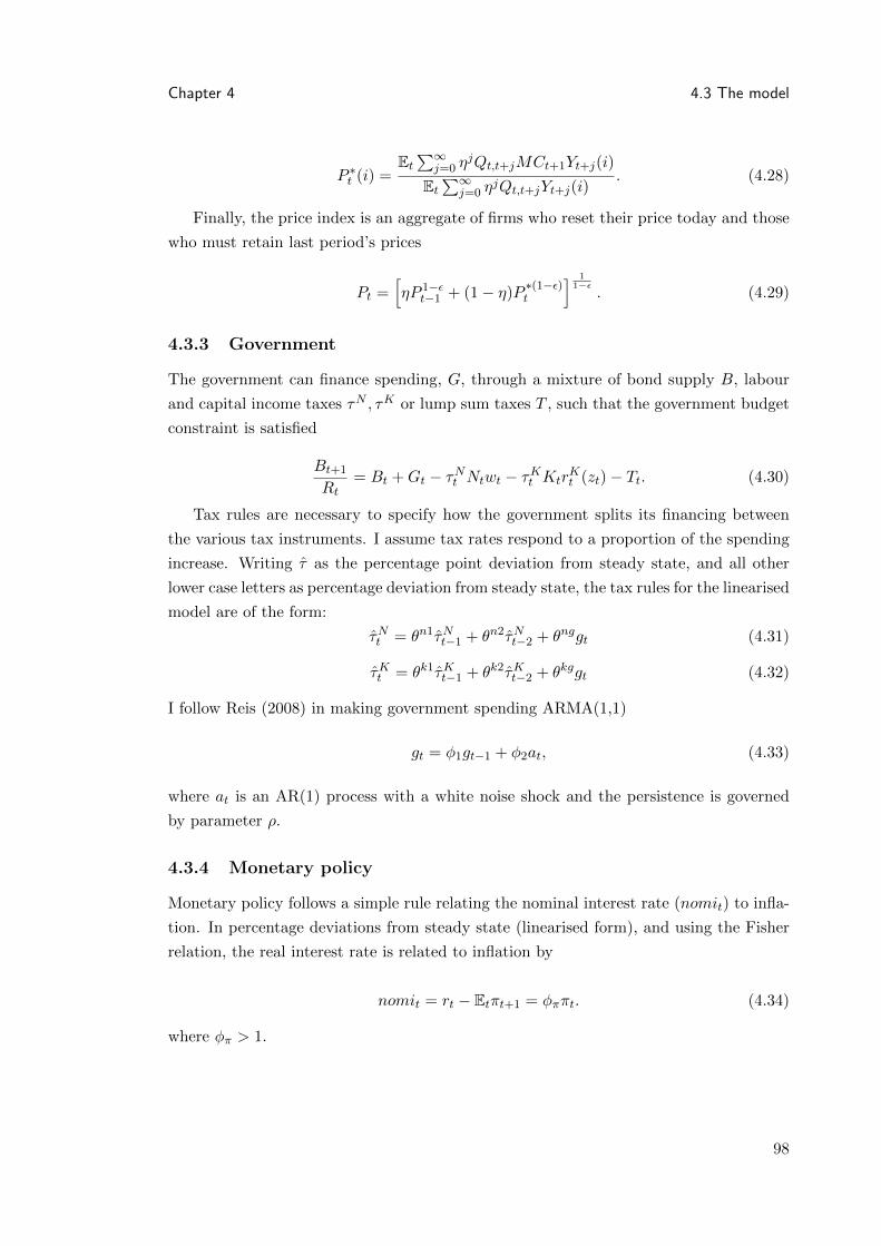
Chapter 4 4.3 The model
P ∗t (i) =Et∑∞
j=0 ηjQt,t+jMCt+1Yt+j(i)
Et∑∞
j=0 ηjQt,t+jYt+j(i)
. (4.28)
Finally, the price index is an aggregate of firms who reset their price today and those
who must retain last period’s prices
Pt =[ηP 1−ε
t−1 + (1− η)P∗(1−ε)t
] 11−ε
. (4.29)
4.3.3 Government
The government can finance spending, G, through a mixture of bond supply B, labour
and capital income taxes τN , τK or lump sum taxes T , such that the government budget
constraint is satisfied
Bt+1
Rt= Bt +Gt − τNt Ntwt − τKt Ktr
Kt (zt)− Tt. (4.30)
Tax rules are necessary to specify how the government splits its financing between
the various tax instruments. I assume tax rates respond to a proportion of the spending
increase. Writing τ as the percentage point deviation from steady state, and all other
lower case letters as percentage deviation from steady state, the tax rules for the linearised
model are of the form:
τNt = θn1τNt−1 + θn2τNt−2 + θnggt (4.31)
τKt = θk1τKt−1 + θk2τKt−2 + θkggt (4.32)
I follow Reis (2008) in making government spending ARMA(1,1)
gt = φ1gt−1 + φ2at, (4.33)
where at is an AR(1) process with a white noise shock and the persistence is governed
by parameter ρ.
4.3.4 Monetary policy
Monetary policy follows a simple rule relating the nominal interest rate (nomit) to infla-
tion. In percentage deviations from steady state (linearised form), and using the Fisher
relation, the real interest rate is related to inflation by
nomit = rt − Etπt+1 = φππt. (4.34)
where φπ > 1.
98

Chapter 4 4.3 The model
4.3.5 Equilibrium and model solution
The equilibrium is defined by an allocation {Kt, Ct, Nt, Yt, Bt, It, zt, Xt}∞t=0, a price system
{wt, Rt, qt, rkt , Pt(i), Pt,mct, λt, µt)}∞t=0, a fiscal policy {τNt , τKt , Gt}∞t=0 and an exogenous
process {at}∞t=0 such that the allocation {Kt, Ct, Nt, Yt, Bt, It, zt, Xt}∞t=0 solves:
1. the households’ problem, maximizing (4.4) subject to (4.5), (4.6), (4.8) and a no-
ponzi condition, given prices, thus satisfying (4.9), (4.10), (4.11), (4.12), (4.13),
(4.14) and (4.15);
2. the firms’ problem (4.27) subject to (4.22) and minimizing costs so that equations
(4.24), (4.25), (4.26), (4.28) and (4.29) are satisfied.
3. All markets clear and equations (4.30), (4.31), (4.32), (4.33) and (4.34) and the
resource constraint Yt = Ct + It +Gt are satisfied.
The equilibrium system is therefore defined by equations (4.6), (4.8), (4.9), (4.10),
(4.11), (4.12), (4.13), (4.14), (4.15), (4.28), (4.29), (4.30), (4.31), (4.32), (4.33), (4.34),
the aggregate production function, the aggregates of equations (4.24), (4.25) and (4.26)
and an exogenous process for at+1 = ρat + εt+1. The set of predetermined variables is
{Bt,Kt, at}.The model is linearised around a deterministic steady state where all firms set the
same price. The collection of linearised conditions can be written in recursive form:
AEt
[xt+1
yt+1
]= B
[xt
yt
](4.35)
where x is the vector of state variables, xt+1 = {kt+1, bt+1, at+1}. y is the vector of
control variables. The solution to this linear rational expectations model is then of the
form:
yt = Qxt (4.36)
xt+1 = Pxt. (4.37)
To solve for matrices P and Q in the policy functions, I employ the Klein (2000) algorithm
solab.
Details of the linearised system and the steady state are given in the Appendices
C.2 and C.3 respectively. Of particular interest are the linearised equations governing
price evolution, utilisation and investment (recall, lower case letters represent percentage
deviations from steady state). The first is the New Keynesian Phillips Curve. Note that
the degree of price stickiness, η, appears in this expression and will be estimated.
πt =(1− βη)(1− η)
ηmct + βEtπt+1. (4.38)
99

Chapter 4 4.4 Key features of the model
Table 4.1: Baseline calibrationParameter Value Description
β 0.99 Discount factorα 0.3 Capital shareδ 0.025 Steady state depreciationτK 0 Steady state capital tax rate (from sample)τN 0 Steady state labour tax rate (from sample)N 0.2 Steady state labourGY 0.2 Steady state share of government spendingBY 1.6 Steady state debt to GDP ratio (quarterly)φπ 1.5 Coefficient on inflation in the monetary policy ruleξ 1.8 Parameter governing the labour supply elasticity (γ = 0)
σ 1 Inverse of elasticity of intertemporal substitution (γ = 1)ρ 0.8 Autoregressive parameter on at shockη 0.75 Probability of having a fixed priceκ 0.15 Parameter governing capital utilisationω 1/3 Parameter governing the investment adjustment costsγ 0.0001 Parameter governing the wealth effecth 0.5 Parameter governing habit persistence
The degree of capital utilisation, zt, is described by
(1 + κ)zt = yt − kt − qt +mct − τKt1
1− τK, (4.39)
where κ = δ′′
δ′ is the elasticity of depreciation to utilisation, and will also be estimated.
Investment evolves according to
qtφ′′
= (1 + β)it − it−1 − βEtit+1 (4.40)
and 1φ′′ = ω will be estimated.
4.4 Key features of the model
In this section I consider some important mechanisms in the model. Before considering
how the choice of tax policy instruments affects the results, I first consider how the
model’s more standard features interact with the strength of the wealth effect on labour
supply under lump sum taxes. Table (4.1) presents the initial baseline calibration for
this section. Parameters in the bottom half of the table will be estimated later.
4.4.1 The strength of the wealth effect on labour supply
Figures (4.3) to (4.7) illustrate the effect of turning on each mechanism one at a time
while still assuming that lump sum taxes fund the spending shock.
100

Chapter 4 4.4 Key features of the model
In Figure (4.3), the model has flexible prices (η = 0), no variable capital utilisation
(κ =∞) and no habit formation (h = 0). γ = 1, so there is a standard wealth effect on
labour supply. This case can therefore be regarded as a simple baseline neoclassical model.
Figure (4.3) shows the familiar neoclassical result. The higher lump sum taxes that
accompany the spending shock lower lifetime wealth, lower consumption, lower savings
and hence investment, but boost labour supply. The real wage therefore falls. Figure
(4.4), however, illustrates the effect of turning off the wealth effect on labour supply, i.e.
setting γ = 0. Labour supply now does not respond to the lower lifetime wealth and
falls as the marginal product of labour declines. Consumption and investment are lower
than before, reflecting the decrease in lifetime wealth and the lack of increased earnings
from supplying more labour. All these forces cause output to fall over time. Importantly,
the neoclassical model can no longer match the empirical output response. In fact the
neoclassical model without a wealth effect on labour supply fails to qualitatively match
any of the output, consumption, real wage or hours responses estimated in Section 4.2.
It is worth emphasising that if the shock were funded with debt rather than lump
sum taxes, Ricardian equivalence implies that the result will be the same. To the extent
that governments rarely, if ever, use lump sum taxes (Chapter 2 and the associated long
appendix documents this for the United Kingdom and see Romer and Romer (2010)
for the U.S.), increased borrowing will be needed to satisfy the government’s budget
constraint (assuming no distortionary taxes). It is therefore an important empirical
question whether debt-finance — which raises expectations about future tax increases —
generates a wealth effect on labour supply today.
101

Chapter 4 4.4 Key features of the model
0 2 4 6 8 10 12−0.1
−0.05
0
0.05
0.1Response of output
% d
evia
tio
n fro
m s
tea
dy s
tate
Output
0 2 4 6 8 10 12−0.2
−0.1
0
0.1Response of consumption
Consumption
0 2 4 6 8 10 12−0.05
−0.04
−0.03
−0.02
−0.01
0
0.01Response of real wages
% d
evia
tion fro
m s
teady s
tate
Real wages
0 2 4 6 8 10 12−0.02
0
0.02
0.04
0.06
0.08
0.1Response of hours worked
Quarters after shock
Hours worked
0 2 4 6 8 10 12
−0.25
−0.2
−0.15
−0.1
−0.05
0
0.05
Response of investment
Quarters after shock
% d
evia
tion fro
m s
tea
dy s
tate
Investment
Figure 4.3: A simple Neoclassical model: η = 0, γ = 1, κ =∞, h = 0
102

Chapter 4 4.4 Key features of the model
0 2 4 6 8 10 12−0.1
−0.05
0
0.05
0.1Response of output
% d
evia
tio
n fro
m s
tea
dy s
tate
Output
0 2 4 6 8 10 12
−0.25
−0.2
−0.15
−0.1
−0.05
0
0.05
Response of consumption
Consumption
0 2 4 6 8 10 12−0.03
−0.02
−0.01
0
0.01Response of real wages
% d
evia
tion fro
m s
teady s
tate
Real wages
0 2 4 6 8 10 12
−0.04
−0.02
0
0.02Response of hours worked
Quarters after shock
Hours worked
0 2 4 6 8 10 12−0.5
−0.4
−0.3
−0.2
−0.1
0
0.1Response of investment
Quarters after shock
% d
evia
tion fro
m s
tea
dy s
tate
Investment
Figure 4.4: A simple Neoclassical model (but no wealth effect): η = 0, γ = 0, κ = ∞,
h = 0
103

Chapter 4 4.4 Key features of the model
Figure (4.5) shows the result of adding sticky prices to the previous model (γ = 0).
This figure illustrates that government spending now has a positive effect on demand
which boosts output, labour demand, the real wage, hours worked and consumption.
The figure also illustrates the Monacelli and Perotti (2009) result that consumption can
rise following the shock. Two features of the model produce this result. Firstly, there is
no wealth effect on labour supply. This means that the real wage does not fall on impact
because the labour supply curve does not shift with the increase in the marginal utility
of wealth. Secondly, in response to the shock, the sticky price demand effect induces an
outward shift of the labour demand curve. For sufficiently sticky prices the result is a rise
in the real wage and hours — raising income enough that consumption also increases.
This effect lowers the amount of dis-saving, lessening the negative effect on investment.
Adding variable capital utilisation to the model serves to amplify these effects slightly,
as can be seen from figure (4.6). Finally, the inclusion of habits adds persistence to the
consumption profile, with additional implications for overall demand. This can be seen
from figure (4.7).
This subsection has shown that all the mechanisms in the model can interact to pro-
duce positive consumption, output, real wage and hours responses, as found empirically
in Section 4.2, depending on the parameter values chosen. This contrasts with the stan-
dard neoclassical model. Limiting the strength of the wealth effect on labour supply
played a key role; the empirical relevance of this mechanism is therefore of particular
importance.
104

Chapter 4 4.4 Key features of the model
0 2 4 6 8 10 12−0.1
0
0.1
0.2
0.3
0.4Response of output
% d
evia
tio
n fro
m s
tea
dy s
tate
Output
0 2 4 6 8 10 12−0.1
0
0.1
0.2
0.3
0.4Response of consumption
Consumption
0 2 4 6 8 10 12−0.1
0
0.1
0.2
0.3
0.4
Response of real wages
% d
evia
tion fro
m s
teady s
tate
Real wages
0 2 4 6 8 10 12−0.1
0
0.1
0.2
0.3
0.4
Response of hours worked
Quarters after shock
Hours worked
0 2 4 6 8 10 12−0.5
−0.4
−0.3
−0.2
−0.1
0
0.1Response of investment
Quarters after shock
% d
evia
tion fro
m s
tea
dy s
tate
Investment
Figure 4.5: Including sticky prices: η = 0.75
105

Chapter 4 4.4 Key features of the model
0 2 4 6 8 10 12−0.1
0
0.1
0.2
0.3Response of output
% d
evia
tio
n fro
m s
tea
dy s
tate
Output
0 2 4 6 8 10 12−0.1
−0.05
0
0.05
0.1
0.15
0.2Response of consumption
Consumption
0 2 4 6 8 10 12−0.1
0
0.1
0.2
0.3Response of real wages
% d
evia
tion fro
m s
teady s
tate
Real wages
0 2 4 6 8 10 12−0.1
0
0.1
0.2
0.3Response of hours worked
Quarters after shock
Hours worked
0 2 4 6 8 10 12
−0.25
−0.2
−0.15
−0.1
−0.05
0
0.05
Response of investment
Quarters after shock
% d
evia
tion fro
m s
tea
dy s
tate
Investment
Figure 4.6: Including variable capital utilization: κ = 0.15
106

Chapter 4 4.4 Key features of the model
0 2 4 6 8 10 12−0.1
0
0.1
0.2
0.3
0.4Response of output
% d
evia
tio
n fro
m s
tea
dy s
tate
Output
0 2 4 6 8 10 12−0.1
0
0.1
0.2
0.3
0.4Response of consumption
Consumption
0 2 4 6 8 10 12−0.1
0
0.1
0.2
0.3Response of real wages
% d
evia
tion fro
m s
teady s
tate
Real wages
0 2 4 6 8 10 12−0.1
0
0.1
0.2
0.3Response of hours worked
Quarters after shock
Hours worked
0 2 4 6 8 10 12
−0.5
−0.4
−0.3
−0.2
−0.1
0
0.1Response of investment
Quarters after shock
% d
evia
tion fro
m s
tea
dy s
tate
Investment
Figure 4.7: Including habits: h = 0.5
107

Chapter 4 4.4 Key features of the model
4.4.2 The effect of different tax instruments
The previous subsection illustrated the importance of the wealth effect on labour supply
under lump sum taxes. This subsection now evaluates the effect of adding distortionary
taxes to the model and explores varying the tax instruments used to finance the shock.
In the above examples, by using lump sum taxes, there were no substitution effects.
This is not true when distortionary taxes finance the spending shock. Figure (4.8) illus-
trates the effect of assuming that the two distortionary tax rates increase following the
spending shock. I also include the results from the full model with only lump sum taxes
in red (dashed) from figure (4.7). For this exercise I arbitrarily choose θgn = θgk = 0.6.
The figure illustrates the strong negative effect on output and consumption of using dis-
tortionary taxes. In short, the results in the previous subsection depend not only on the
strength of the wealth effect on labour supply, but also — quite dramatically — on the
instruments used to finance the shock. I now consider the two types of taxes individually.
Labour income taxes
Consider the supply side effects of a rise in the labour income tax rate. There are two
substitution effects. First, the intra-temporal decision is distorted and labour supply falls.
In other words, it is more costly to supply labour today as the worker pays higher taxes
per hour. Second, the inter-temporal decision is distorted if the tax rate is changing over
time (as it may be when the tax rules are estimated). For a rising (falling) tax profile the
worker may still prefer (dislike) to work today as it will be relatively less (more) costly
than tomorrow. These substitution effects work to offset the wealth effect on labour
supply. In the simulations below, labour supply falls considerably following a rise in
government spending.
To illustrate the effect, I calibrate the coefficient on gt in the labour tax rule to be
0.95, leaving the equivalent parameter zero in the capital tax rule. Figure (4.9) shows
the strong negative effect of this change in the tax policy rule. Again, the results from
the model with only lump sum taxes are shown in red (dashed). The positive effects on
output, consumption and hours in the previous subsection are now reversed when labour
income taxes finance the shock.
Capital income taxes
Figure (4.10) shows the effect of calibrating the coefficient on gt in the capital tax rate
rule to 0.95, leaving the equivalent coefficient zero in the labour tax rule. Again, results
from the model with only lump sum taxes is shown in red (dashed).
Interestingly, the use of capital taxes raises consumption and output on impact but
lowers the persistence. This effect is a combination of substitution effects and sticky
prices (and habits). Taxing capital makes consumption relatively more attractive than
108

Chapter 4 4.4 Key features of the model
saving. As a result, ceteris paribus, the balance between consumption and saving tilts
towards consumption. This increase in demand, given sticky prices, boosts output in the
short run. With flexible prices the increase in capital taxes tends to lower consumption
and output as the capital stock declines.
Another key determinant of the size of this response is the presence of capital adjust-
ment costs. The distortions introduced by taxing capital are not fully felt immediately
but become apparent over time as the capital stock adjusts. This explains the decline in
output over time.
Summary
The previous subsections have analysed the interactions between debt finance/lump sum
taxes, the use of distortionary taxes and the wealth effect channel. Debt finance (or lump
sum taxes) minimises the contemporaneous distortions associated with labour and capital
taxes. Labour income taxes produce a strong negative effect on all the key variables. If
the objective is a stimulus to output (rather than a concern with welfare), this suggests
labour income taxes should be avoided. The use of capital income taxes may raise the
impact stimulus by boosting consumption but will lower the persistence of the effect on
output as the capital stock declines faster.
I also showed that with debt-finance (or lump sum taxes) the model’s predictions
rest on the strength of the wealth effect on labour supply and the degree of price sticki-
ness (and, to a lesser extent, habits and variable capital utilisation, which reinforce the
results). A low degree of wealth effect on labour supply allows the sticky price effects
to jointly raise output, consumption, the real wage and hours. However, for stronger
degrees of wealth effect, consumption will fall. Conversely, if the wealth effect is small,
but prices are flexible, output and consumption both fall.
In short, this section has shown that the choice of tax policy instruments matters, as
does the strength of the wealth effect on labour supply. In fact, the model’s results are
highly dependent on these parameters. However, there is no a priori reason to calibrate
either the tax policy rules in a particular way or to assume a particular strength of
wealth effect on labour supply. To properly evaluate the ability of the model to explain
the effects of a government spending shock, arbitrarily calibrating these key parameters
will not be enlightening. Estimation is therefore the most appropriate strategy to follow.
109

Chapter 4 4.4 Key features of the model
0 2 4 6 8 10 12−0.5
0
0.5Response of output
% d
evia
tio
n fro
m s
tead
y s
tate
0 2 4 6 8 10 12
−0.4
−0.2
0
0.2
0.4Response of consumption
0 2 4 6 8 10 12
0
0.2
0.4
0.6
0.8
1Response of real wages
% d
evia
tio
n f
rom
ste
ad
y s
tate
0 2 4 6 8 10 12−0.5
0
0.5Response of hours worked
Quarters after shock
0 2 4 6 8 10 12−1
−0.8
−0.6
−0.4
−0.2
0
Response of investment
Quarters after shock
% d
evia
tion fro
m s
teady s
tate
Figure 4.8: Distortionary labour and capital tax rates respond (full model with lump sum
taxes in red (dashed))
110
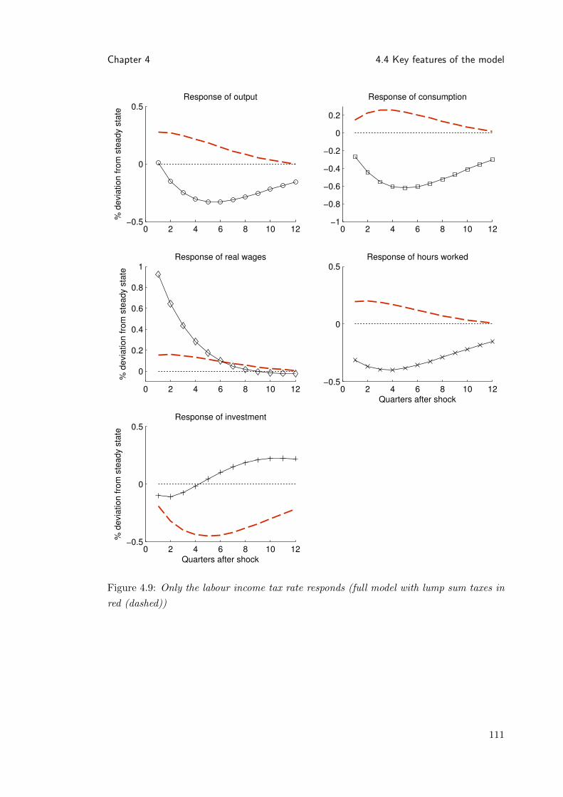
Chapter 4 4.4 Key features of the model
0 2 4 6 8 10 12−0.5
0
0.5Response of output
% d
evia
tio
n fro
m s
tead
y s
tate
0 2 4 6 8 10 12−1
−0.8
−0.6
−0.4
−0.2
0
0.2
Response of consumption
0 2 4 6 8 10 12
0
0.2
0.4
0.6
0.8
1Response of real wages
% d
evia
tio
n f
rom
ste
ad
y s
tate
0 2 4 6 8 10 12−0.5
0
0.5Response of hours worked
Quarters after shock
0 2 4 6 8 10 12−0.5
0
0.5Response of investment
Quarters after shock
% d
evia
tion fro
m s
teady s
tate
Figure 4.9: Only the labour income tax rate responds (full model with lump sum taxes in
red (dashed))
111

Chapter 4 4.4 Key features of the model
0 2 4 6 8 10 12
−0.2
−0.1
0
0.1
0.2
0.3
0.4
Response of output
% d
evia
tio
n fro
m s
tead
y s
tate
0 2 4 6 8 10 12
0
0.2
0.4
0.6
0.8Response of consumption
0 2 4 6 8 10 12−0.1
0
0.1
0.2
0.3
0.4
Response of real wages
% d
evia
tio
n f
rom
ste
ad
y s
tate
0 2 4 6 8 10 12
0
0.2
0.4
0.6
0.8Response of hours worked
Quarters after shock
0 2 4 6 8 10 12−3
−2
−1
0
1Response of investment
Quarters after shock
% d
evia
tion fro
m s
teady s
tate
Figure 4.10: Only the capital tax rate responds (full model with lump sum taxes in red
(dashed))
112
Chapter 4 4.5 Estimation
4.5 Estimation
I estimate the model using a minimum distance approach as discussed by, for example,
Christiano et al. (2005). Key parameters of the model are chosen to minimize the distance
between the model’s impulse responses and the empirical impulse responses.
The model’s parameters are partitioned into two blocks. The first block includes
a set of parameters which are calibrated. The second block includes parameters to be
estimated. I estimate all the parameters of the fiscal policy rules. I also estimate the
parameters of the key mechanisms in the model: γ governing the size of the wealth effect,
κ determining the degree of variable capital utilisation, ω determining the strength of the
investment adjustment costs, η the degree of price stickiness and the habit persistence
parameter h. The parameter vector to be estimated is therefore11
ζ = [φ1 φ2 θgn θn1 θn2 θgk θk1 θk2 η κ γ h ω].
Let the empirical impulse responses be stacked in a vector x. The model produces
impulse responses conditional on a set of parameters. Let the parameter vector be ζ as
above. Let the output of the model given the set of parameters be x(ζ). The objective
is to choose parameters to minimise the loss function
ζ = arg minζ
[x− x(ζ)]V −1[x− x(ζ)]′, (4.41)
where V is a weighting matrix which includes the variances of the empirical impulses
along the diagonal and zeros elsewhere. The purpose of this matrix is to down-weight
observations with larger standard errors. As such, I ensure that the estimated model’s
responses lie as far inside the empirical confidence intervals as possible.
I match the model’s impulse responses to the first 16 periods of the nine empirical
impulse responses. Dropping any observation with zero variance from the loss function
(the first element of the government spending series) leaves the x vectors ((9×16)−1)×1
and the V matrix ((9× 16)− 1)× ((9× 16)− 1) in dimension.
The standard errors are calculated following Hall et al. (2010). Specifically the
variance-covariance matrix of the estimated parameters is found as the solution to:
Vζ =
[∂x(ζ)
∂ζ
′W−1∂x(ζ)
∂ζ
]−1
(4.42)
where W is the variance-covariance matrix of the impulse response functions and ∂x(ζ)∂ζ
is the ((9× 16)− 1)× 9 Jacobian of the theoretical impulse responses with respect to the
parameter vector.
11For a list of parameter definitions see table (4.2).
113

Chapter 4 4.5 Estimation
4.5.1 Results
The estimated parameter values are given in table (4.2). The tax rate responses to
the government spending shock are estimated to be small, although the response builds
over time — as can be seen from the coefficients on the lagged tax rates. Figure (4.11)
displays the matched policy responses implied by the estimated model, together with
the confidence intervals from the SVAR. The estimated fiscal policy parameters in table
(4.2) generate responses within the empirical confidence intervals and are thus a decent
replication of the empirical policy response. For reference, I also plot the simulated
debt path from the model given the spending and tax rate changes. Interestingly, based
on the model’s estimated parameters, these tax rate changes are consistent with the
empirically estimated response of debt from Section 4.2. This suggests that spending
shocks are typically funded more through debt than through contemporary tax changes,
again mirroring results found in Chapter 3.
Table (4.2) also reports the other estimated parameter values and their standard
errors. It is worth comparing these with values discussed elsewhere. King and Rebelo
(1999) take κ ∈ [0.1,∞] and the value in table 4.2 is close to the value of 0.15 used
by Jaimovich and Rebelo (2009). η is of the order of magnitude usually used in New
Keynesian models and is similar to the value of 0.82 estimated by Altig et al. (2005). It
is, however, slightly too high, which may suggest other amplification mechanisms could
be included in the model to lower the required degree of price stickiness. The estimate
for γ implies a very small wealth effect on labour supply and not statistically significant
from zero. This reinforces the results of Schmitt-Grohe and Uribe (2010). h is similar
to the value of 0.7 used by Monacelli and Perotti (2009) and is a fairly standard figure
found in the wider literature. These estimates are also similar to those found in Chapter
3.
Figure (4.12) displays the responses of the other key macroeconomic variables. Again,
the estimated model produces responses largely within the confidence intervals. It is
noteworthy that the estimated model jointly replicates the output and consumption
responses, which is often a problem for New Keynesian models. Although the hours
response is slightly too strong, most of the real wage response is well matched. The
investment response is too shallow to start with and too strong over time; however this
reflects the investment adjustment cost mechanism. The parameter less well estimated
is ω, which governs the investment adjustment costs. The estimate is well below the
value of 1/8 estimated by Mertens and Ravn (2011b), which itself is lower than in other
studies. However, raising the value of ω would produce too great a decline in investment.
All this suggests interesting scope for considering more complicated investment dynamics
in the transmission of fiscal shocks.
114

Chapter 4 4.5 Estimation
Table 4.2: Estimated parameter values
Parameter Estimation Description
ρ 0.94 (0.02) Persistence of shock processφ1 0.00 (0.08) Persistence of spending processφ2 -0.14 (0.06) Effect of shock on spendingθgn 0.0043 (0.02) Contemporaneous response of the labour tax rateθgk 0.0046 (0.002) Contemporaneous response of the capital tax rateθn1 0.19 (0.1) Labour tax rate AR(1) coefficientθk1 1.87 (0.07) Capital tax rate AR(1) coefficientθn2 0.038 (0.1) Labour tax rate AR(2) coefficientθk2 -0.91 (0.07) Capital tax rate AR(2) coefficientγ 0.0023 (0.003) Strength of the wealth effecth 0.58 (0.06) Strength of habitsη 0.86 (0.04) Probability of a fixed priceκ 0.16 (0.33) Governs capital utilisationω 0.032 (0.03) Governs investment adjustment costs
Loss 51.52
Government Spending
0 2 4 6 8 10 120
0.2
0.4
0.6
0.8
1Labour taxes
0 2 4 6 8 10 12−0.2
−0.1
0
0.1
0.2
Capital taxes
0 2 4 6 8 10 12
−0.2
−0.1
0
0.1
0.2
0.3Debt
0 2 4 6 8 10 12−1
−0.5
0
0.5
1
Figure 4.11: Responses of the fiscal variables given the parameter estimates
115

Chapter 4 4.5 Estimation
Output
0 2 4 6 8 10 12−0.2
−0.1
0
0.1
0.2
0.3
0.4
Consumption
0 2 4 6 8 10 12−0.2
−0.1
0
0.1
0.2
0.3
0.4
Investment
0 2 4 6 8 10 12−1
−0.5
0
0.5
1Labour
0 2 4 6 8 10 12−0.2
−0.1
0
0.1
0.2
0.3
0.4
Wage
0 2 4 6 8 10 12−0.2
−0.1
0
0.1
0.2
0.3
0.4
Figure 4.12: Responses of the other variables given the parameter estimates
116

Chapter 4 4.5 Estimation
4.5.2 Robustness
I now examine the robustness of the parameter estimates when each of the main mech-
anisms discussed earlier are turned off or directly calibrated.12 Table (4.3) displays the
results from these experiments.
First consider the fiscal policy parameters. Estimates of the persistence of the gov-
ernment spending process (ρ and φ1) are very similar across all specifications. So too is
the impact response of the tax rates following the spending shock (θgk and θgn). The
persistence coefficients in the tax rules do vary somewhat, although these estimates still
produce impulse responses generally within the empirical confidence intervals.
In all cases the strength of the wealth effect on labour supply is estimated to be
low. This mirrors findings by Schmitt-Grohe and Uribe (2010). Furthermore, note that
the loss increases significantly when γ is forced to be one, the case of King-Plosser-
Rebelo-type preferences. The degree of price stickiness is estimated to be high across
all specifications, suggesting an important role for short-run demand effects. However,
when other mechanisms are turned off — notably variable capital utilisation — the
degree of price stickiness becomes implausibly high. It is also interesting to note that the
flexible price model (where η = 0) does not perform too badly (in terms of loss). This,
however, relies on an implausibly high level of variable capital utilisation and strong habit
persistence. Similarly, estimates of the habit persistence parameter increase significantly
when sticky prices or variable capital utilisation are turned off. In general, the parameter
estimates governing variable capital utilisation and the investment adjustment costs, κ
and ω, are far too low. These experiments did not, therefore, resolve the issues with the
investment response discussed earlier.
These exercises confirm several important results. Firstly, that the strength of wealth
effect on labour supply is robustly low across all specifications. Secondly, that the
strength of the tax rate response to government spending shocks is limited. And, thirdly,
all the model’s mechanisms appear important for matching the empirical evidence: the
baseline case achieves the smallest loss.
12Parameter values used in table (4.3) reflect commonly chosen values elsewhere in the literature.
117

Chapter 4 4.5 Estimation
Tab
le4.
3:R
obu
stn
ess
ρφ
1φ
2θgn
θgk
θn1
θk1
θn2
θk2
γh
ηκ
ωL
oss
Bas
elin
e0.
940.0
0-0
.14
0.00
430.
0046
0.19
1.87
0.03
8-0
.91
0.00
230.
580.
860.
160.
032
51.5
2(0
.02)
(0.0
8)
(0.0
6)
(0.0
2)
(0.0
02)
(0.1
)(0
.07)
(0.1
)(0
.07)
(0.0
03)
(0.0
6)
(0.0
4)
(0.3
)(0
.03)
Fix
edh
abit
s0.
920.0
003
-0.0
100.
0021
0.00
340.
077
1.94
-0.0
93-0
.97
0.02
7-
0.88
0.00
0.05
060
.25
(h=
0.6
)(0
.02)
(0.0
7)
(0.0
6)
(0.0
2)
(0.0
02)
(0.1
)(0
.07)
(0.1
)(0
.07)
(0.0
1)
(0.0
3)
(0.0
3)
(0.0
5)
No
hab
its
0.93
0.0
002
-0.0
120.
021
0.03
90.
012
-0.0
63-0
.041
0.81
0.00
42-
0.91
0.00
0.00
1996
.04
(h=
0)
(0.0
1)
(0.0
6)
(0.0
5)
(0.0
2)
(0.0
1)
(0.0
7)
(0.0
6)
(0.0
7)
(0.0
7)
(0.0
1)
(0.0
2)
(0.0
8)
(0.0
2)
Fix
edu
tili
sati
on
0.92
0.0
024
-0.0
140.
013
0.00
430.
029
1.89
0.16
-0.9
30.
0044
0.55
0.85
-0.
029
56.1
6(κ
=0.1
5)
(0.0
2)
(0.0
7)
(0.0
6)
(0.0
2)
(0.0
02)
(0.1
)(0
.06)
(0.1
)(0
.07)
(0.0
04)
(0.0
4)
(0.0
3)
(0.0
3)
No
uti
lisa
tion
0.93
0.0
11
-0.1
00.
025
0.00
160.
054
2.00
0.00
90-1
.00
0.06
90.
940.
97-
0.01
480
.29
(κ=∞
)(0
.01)
(0.0
7)
(0.0
5)
(0.0
1)
(0.0
01)
(0.0
05)
(0.0
01)
(0.0
02
)(0
.001)
(0.0
002)
(0.0
005)
(0.0
07)
(0.0
09)
Fix
edad
j.co
sts
0.93
0.0
0-0
.042
0.03
00.
0027
-0.3
41.
970.
35-1
.00
0.04
10.
860.
970.
087
-54
.96
(ω=
1/3)
(0.0
1)
(0.0
7)
(0.0
5)
(0.0
2)
(0.0
01)
(0.0
7)
(0.0
9)
(0.0
8)
(0.0
9)
(0.0
2)
(0.0
7)
(0.0
8)
(0.0
9)
Fix
edη
=0.
750.
920.0
00.
0094
0.01
00.
026
-0.1
0-0
.020
0.20
0.93
0.06
10.
89-
0.00
240.
0077
60.6
4(0
.02)
(0.0
7)
(0.0
5)
(0.0
2)
(0.0
1)
(0.0
8)
(0.0
4)
(0.0
6)
(0.0
8)
(0.0
2)
(0.0
3)
(0.0
4)
(0.0
07)
Fle
xib
lep
rice
s0.
920.0
016
0.01
60.
027
0.02
20.
012
0.04
2-0
.021
0.92
0.06
10.
88-
0.00
0.01
064
.93
(η=
0)
(0.0
2)
(0.0
7)
(0.0
6)
(0.0
2)
(0.0
1)
(0.1
)(0
.03)
(0.1
)(0
.09)
(0.0
2)
(0.0
5)
(0.0
4)
(0.0
08)
γ=
0.01
0.92
0.0
0-0
.024
0.00
540.
0036
0.07
61.
910.
0051
-0.9
4-
0.56
0.87
0.00
0.03
253
.98
(0.0
2)
(0.0
7)
(0.0
6)
(0.0
2)
(0.0
01)
(0.1
)(0
.06)
(0.1
)(0
.06)
(0.0
8)
(0.0
3)
(0.0
5)
(0.0
3)
γ=
10.
910.0
00.
041
0.02
40.
0023
0.02
61.
970.
14-1
.0-
0.18
0.92
0.00
0.11
125.
42(0
.01)
(0.0
7)
(0.0
6)
(0.0
2)
(0.0
01)
(0.2
)(0
.06)
(0.2
)(0
.06)
(0.3
)(0
.02)
(0.0
4)
(0.2
)
118

Chapter 4 4.6 Conclusion
4.6 Conclusion
In this chapter I have empirically investigated the importance of the endogenous tax
response to government spending shocks and the strength of the wealth effect channel in
the United States. The estimated model matches well the empirical effects of an increase
in government spending, with parameter estimates largely in line with those estimated
elsewhere in the literature.
The mix of tax policy instruments matters greatly for the sign and magnitude of
key responses. For example, greater use of labour income taxes causes a contraction in
output, consumption, the real wage and hours, all contrary to the empirical evidence
presented in Section 4.2.
Furthermore, the degree of distortionary tax finance interacts with the strength of the
wealth effect on labour supply, which can partially offset any negative substitution effects.
By employing Jaimovich and Rebelo (2009) preferences, I showed that the neoclassical
model with a low wealth effect on labour supply fails to match the output, consumption,
real wage or hours responses found in the SVAR evidence. The presence of sticky prices,
however, allows the model to qualitatively match all the empirical responses. The model
also contains more standard features such as variable capital utilisation, investment ad-
justment costs and habits. All these played a role in replicating the empirical evidence. I
showed how these mechanisms interact and this motivated estimation of the parameters
governing their strength. This is particularly important given that there is little, if any,
a priori information for calibrating the tax rules or the strength of the wealth effect.
The key findings that allow the estimated model to replicate the empirical impulse
responses are, first, that the wealth effect on labour supply is estimated to be small. This
casts further doubt on whether a simple neoclassical model can replicate the empirical
evidence. Second, sticky prices, variable capital utilisation, investment adjustment costs
and habits were all found to play an important role, with parameter values generally in
line with those found in the wider literature. One exception is the parameter govern-
ing the investment adjustment costs. Typical calibrations of this parameter would have
implied a larger fall in investment than was observed in the empirical results. My re-
sults suggest that further work should be done to investigate the response of investment
following a government spending shock. Third, I find that while distortionary tax rates
rise following the spending shock, their magnitudes are modest. Importantly, capital tax
rates increase more than labour tax rates, limiting the contractionary effect on output
and consumption. The model also implies a realistic debt path on the basis of these tax
rate changes, implying that government spending shocks — at least over the short to
medium-term horizon — tend to be debt-financed.
To the extent that nominal rigidities allow for short-run demand effects and, to the
extent that the wealth effect on labour supply is small, my results suggest that debt-
financed (or lump sum tax financed) government spending shocks will stimulate output,
119

Chapter 4 4.6 Conclusion
consumption, hours and the real wage over the short term. The output multiplier was
around one. However, the decline in investment is important as it lowers the econ-
omy’s longer-term output and wealth. Furthermore, the required current and future
tax increases place a welfare cost on the economy, even if consumption and output rise
initially. The short-term gain of a spending stimulus then has to be traded-off against
the long-term costs. Striking this balance clearly remains hugely topical in the current
climate.
120

Appendices
121

Appendix A
Appendices to Chapter 2
A.1 Long Appendix to Chapter 2: The Narrative Paper
122

Discretionary Tax Shocks in the United Kingdom 1945-2009: A
narrative account and dataset
Summary This appendix constructs a narrative account of all legislated discretionary policy changes in
the United Kingdom from 1945 to 2009. Following Romer and Romer (2009, 2010), evidence
of the policymakers’ motivation is presented from U.K. official Budget documents together
with technical notes, press releases, Acts of Parliament, the Budget speech by the Chancellor
of the Exchequer and related entries in the parliamentary record (Hansard). The historical
context in which the decision was made is also discussed. Using the given motives I isolate tax
policy changes which were not responding to, or influenced by, current or prospective
economic shocks. This ‘exogenous’ category is comprised of actions to improve long-run
economic performance, those motivated by ideological or political reasons, rulings from
external bodies such as courts, and fiscal consolidation measures based on long-run
considerations. By contrast, the ‘endogenous’ changes are actions to manage demand, to
stimulate production, to offset a debt crisis and those to fund spending decisions. For all the
tax changes I collect information on the announcement, implementation and withdrawal dates
as well as the type of the tax (such as income tax). The dataset contains nearly 2,500 tax
changes and is aggregated into a quarterly series for analysis. In addition to creating a novel
dataset this appendix also contributes to the post-war history of U.K. taxation.
Appendix A A.1 Long Appendix to Chapter 2: The Narrative Paper
123

Introduction As noted in Chapter 2, despite its importance for current macroeconomic policymaking,
evidence of the macroeconomic effects of tax shocks in the United Kingdom is sparse.
Furthermore, while the academic literature has focused on the United States and cross country
panel datasets, there is no consensus of the effects of tax changes. This reflects the difficulty of
identifying tax policy shocks uncorrelated with, and uncontaminated by, other fluctuations.
One major problem with common tax measures is simultaneity. Changes in taxes are likely to
contemporaneously affect GDP but commonly used tax variables such as tax revenues are also
contemporaneously driven by GDP.
Despite the importance of resolving this identification problem, current approaches are
limited. One popular method is that of Blanchard and Perotti (2002). This seeks to cyclically
adjust the change in overall revenues, net of transfers, for changes in GDP. The method
assumes policymakers are not informed about, or are unable to respond to, shocks within the
same quarter. External information is used to calibrate the elasticity of output to GDP. A
residual term can then be constructed and, under the timing assumptions, it can be interpreted
as the discretionary policy decisions uncorrelated with other fluctuations. However, this
approach is not without its problems. First, the timing assumptions may not hold in reality.
Second, we need to be confident that revenues have been adjusted for all the possible cyclical
influences. As many factors are likely to affect revenues, it is unclear what a comprehensive
list would be. Third, legislated tax shocks are not simply shocks to revenues; they alter rates
and liabilities, which themselves are likely to affect the output elasticity which Blanchard and
Perotti (2002) assume to be constant.
This appendix addresses the identification problem directly by constructing a new
measure of the tax policy shocks in the United Kingdom that should be uncorrelated with
current or projected economic fluctuations. The source for this dataset is the narrative record in
the United Kingdom. I therefore pursue a narrative identification approach following Romer
and Romer (2010). Other ‘narrative approaches’ have also been used to identify government
spending shocks (Ramey and Shapiro (1998); Ramey (2011)) and monetary policy shocks
(Romer and Romer (1989, 2004)).
To construct the narrative dataset, the first step is to collect direct measures of all the
legislated tax policy changes in the United Kingdom between 1945 and 2009. The main source
for these data is the official Budget documents. I then employ the Romer and Romer (2010)
strategy of classifying tax changes by motivation. This allows me to identify those decisions
that were taken for reasons uncorrelated with current or prospective economic conditions. I
follow Romer and Romer (RR) in calling these actions ‘exogenous’ tax changes. Actions
which do not satisfy this criteria are referred to as ‘endogenous’.
There are nearly 2,500 discretionary policy changes over the period. Each Budget
usually had both overall objectives as well as individual motivations for the specific measures.
Motives for all discretionary changes are collected from sources such as the Budget speech by
the Chancellor of the Exchequer and related entries in the parliamentary record (Hansard). A
variety of motives are given for actions and I divide the exogenous and endogenous groups
Appendix A A.1 Long Appendix to Chapter 2: The Narrative Paper
124

into subcategories. In doing so, I keep as close as possible to the stated motivation. This
generates slightly different subcategories from those in RR. The ‘exogenous’ category is split
into actions to improve long-run economic performance, ideological changes related to party
political or social causes, rulings from external bodies such as courts, and fiscal consolidation
measures based on long-run considerations. The endogenous changes contain actions to
manage demand, to stimulate production, to offset a debt crisis and those to fund spending
decisions.
In addition to classifying each discretionary policy action, I also collect information on
their announcement dates, their implementation and end dates, their revenue effects and their
type (e.g. income tax). In the narrative below I present evidence for the classification of all the
major changes. I also provide an historical context, informed both by the policymakers’ own
statements and the history literature.
By constructing a new measure of tax changes for the United Kingdom this appendix
provides a rich new dataset dealing with the identification problem. The constructed series is
so useful precisely because it isolates the policy changes which are uncorrelated with current
and prospective economic shocks. This then facilitates further research for a country where
surprisingly little is known about the macroeconomic effects of tax changes. In Chapter 2 I
make use of this new dataset.
A number of factors make the U.K. ideal for a narrative approach. Firstly, the U.K.
has made considerable use of fiscal policy post-war. Secondly, tax policy is highly centralised1
and, since the Budget is a major annual event, tax changes are largely saved for this
announcement with implementation taking place throughout the year. Moreover, unlike in the
United States, these announcements almost always become law. Thirdly, detailed revenue
forecasts are provided for all the Budget measures. Fourthly, given the extensive political
debate around the Budget, there is considerable discussion of the motives.
The central contribution of this appendix is to provide a new measure of tax shocks in
the United Kingdom. The first part of this appendix discusses the construction of the new
dataset. I also discuss the more technical details, the assumptions made and how the 2,500
changes are aggregated. The second part of this appendix then presents the narrative
chronologically by Budget. For each Budget I consider the historical context in which the
policymakers’ decisions were made. I then present evidence on the overall objectives and
motivation, followed by evidence of the specific motives for individual measures.
Instruments and implementation of tax policy in the United Kingdom The centrepiece of the British tax process is the annual Budget. This is a traditional and grand
occasion which attracts extraordinary media coverage in spite of its technical nature. Part of
the attraction is the rhetoric and theatre of the Budget speech as well as the anticipation of
surprises Chancellors invariably try to pull out of their hat. However, the Budget is more than
pomp and circumstance; it is also the annual presentation of the Government’s economic
policy. The policy changes are — with the exception of emergency measures and recently a
1 Adam et al. (2010) note that only 5 per cent of revenue is raised locally.
Appendix A A.1 Long Appendix to Chapter 2: The Narrative Paper
125

second Budget-type event in the autumn (the Pre-Budget Report) — stored up for this
performance. This process and the other features mentioned in the introduction make the U.K.
ideal for a narrative study of tax changes.
On Budget day the Chancellor of the Exchequer – the U.K.’s Finance Minister –
presents the Government’s Budget to the House of Commons of the United Kingdom
Parliament. The speech usually contains a review and analysis of the economic situation
together with the announcement of most of the policy changes. Many publications accompany
the Budget speech. These include a comprehensive review of the policy changes in the
Financial Statement and Budget Report (FSBR),2 the ‘Red Book’. There are also a large
number of press releases and technical notes. I discuss the specific sources below.
The implementation of most Budget changes is legislated in the annual Finance Bill.
This is usually presented on the same day as the Budget and is debated and reviewed by
Parliament over the following months. For a March or April Budget, the Finance Bill usually
becomes an Act of Parliament and receives ‘Royal Assent’ (by the Head of State) in July or
August. Parliament is allowed to revise the Finance Bill and, on occasion (though rarely), this
has led to major Budget measures being added or removed. Some policy changes can also be
implemented before the passing of the Finance Bill. The approval of Budget Resolutions
permits this to take place. Resolutions are tabled as soon as the Chancellor has finished the
speech.3
Technically some taxes are permanent, such as all indirect taxes; others require annual
renewal. As every Budget tends to carefully justify all the policy changes, the announcement
of annual taxes feels much more permanent than this distinction might suggest. For example,
when income taxes are raised the tone of the Budget assumes that this is a permanent rise (until
otherwise determined), even if technically the rate would have to be ‘renewed’ the following
year. As a rule I do not consider these annual taxes as temporary changes. I discuss the
temporary/permanent distinction below, as well as taxes which are automatically renewed or
implemented (such as those required to rise in line with inflation).
The process for emergency or supplementary Budgets is similar to the process above.
Sometimes there was more than one Budget per year and sometimes there were various mini-
Budgets altering specific taxes. In the 1980s there was an Autumn Statement which dealt with
spending and social security changes. Since 1997 there has also been a Pre-Budget Report in
the autumn which, over time, closely to resemble a Budget (although many of the changes in
the PBR were scheduled for the following year’s Finance Bill).
It is useful at this stage to discuss Social Security contributions. Historically the U.K.
has maintained a ‘Contributory Principle’ towards welfare: citizens contributed to the National
Insurance Fund through National Insurance (Social Security) contributions. However, a House
of Commons review in 2000 into Social Security stated “National Insurance contributions are
increasingly described by the Government as a form of taxation”.4 Furthermore, the Institute
2 Before 1969 this was simply called the Financial Statement and in many years a separate Economic Survey was published. 3 Some changes can also be made at a later date by Statutory Instruments (secondary legislation). 4 Select Committee on Social Security Fifth Report (2000).
Appendix A A.1 Long Appendix to Chapter 2: The Narrative Paper
126

for Fiscal Studies (IFS) (2009) explains: “the link between the amount contributed and the
benefit entitlement, which was once close, has now almost entirely gone and substantial
progress has been made in aligning the NI rate structure and tax base with those of income tax.
Most of this has occurred in the last 25 years”. 5 The point about the “last 25 years” can be
clearly seen in the Budgets themselves. Until the mid-1970s it was common for the Chancellor
to simply state that benefits would be going up but that the Secretary of State for Social
Security would shortly be announcing changes in contributions to fund this (usually in the
annual review of contributions, which also responded to the Government Actuaries’ report on
the National Insurance Fund).
At least in theory, the funding of Social Security was supposed to be different from the
standard Budget process. However, from about the mid-1970s (for example, the National
Insurance Surcharge in the mid-1970s was not designed to top up the Fund) changes in
National Insurance have been increasingly made in the Budget and their character has more
closely resembled changes in taxation. In the 1980s National Insurance was widely reformed
— as the IFS note — and these changes were implemented within the Budget process. By the
2000s National Insurance changes were treated in the Budget in a similar way to income tax.
Circumstantial evidence of this can be seen from the 2010 General Election debate which
focused on whether National Insurance should rise to help reduce the Budget deficit in the
future. When part of the Budget process, I include these National Insurance changes. I am
therefore implicitly categorising the other changes as endogenous and spending-driven (see
below).
Data Sources I collect data on the forecast change in revenues resulting from discretionary changes in tax
policy. The main source for these data is the so-called Budget Red Book published by Her
Majesty’s Treasury (H.M. Treasury). Before 1969 this was called the Financial Statement
before becoming the Financial Statement and Budget Report (FSBR, which contained
economic analysis as well as data). Since 1997 there has also been an Economic and Fiscal
Strategy Report (EFSR). The FSBR contains a key table with projected revenue estimates of
all discretionary policy changes. In later years it contained as many as 85 changes and in total
there were about 2,500 non-negligible6 changes in taxation between 1945 and 2009.
Taxes were, on occasion, altered between Budgets. There are several ways of
uncovering these changes. In some cases they appeared in the following year’s FSBR; some
were referred to in a Budget speech; and some were discussed in the Economic Survey (for the
early years) or the EFSR (since 1997). However, to avoid missing policy changes, I also made
use of the history literature. Four useful texts were Christopher Dow’s “The Management of
the British Economy 1945-60”, Alec Cairncross’s “The British Economy since 1945”, Andrew
Britton’s “Macroeconomic Policy in Britain 1974-87” and Nicholas Woodward’s “The
5 IFS (2009), “A Survey of the UK Tax System”, Briefing Note No.9. 6 The definition of a negligible action is made by Her Majesty's Treasury (HM Treasury) and no public figure is then given for these policy changes. In 2009 for example, this was a change amounting to less than 0.0002 per cent of GDP.
Appendix A A.1 Long Appendix to Chapter 2: The Narrative Paper
127

management of the British economy 1945-2001”. Woodward and Dow include a chronology
with the dates of all major policy announcements as well as key economic events. Using all
these sources I am confident that I have accounted for all the tax changes between Budgets.
To establish the implementation date of a change I normally use the FSBR (and if
different from Budget day, an announcement date is also given). In some cases the
implementation date is not reported. I then look directly at the Finance Act itself (or, in some
cases, the relevant Statutory Instruments) or technical notes and press releases. Sometimes the
implementation date is the date of passing of the Act (‘Royal Assent’) but this is not usually
the case.
To categorise the motivations behind the policy changes I primarily use the
Chancellor’s Budget speeches and Hansard debates. These discuss the overall Budget
objectives and strategy, the policy context and motivations for individual measures. It is
typical in U.K. Budget speeches to announce most, if not all, the measures. In addition, there
are other sources which proved useful. In later years the Economic and Fiscal Strategy Report
provided significant justification and motivation — and this proved more useful than the
Budget speeches after 1997. I also used the Economic Surveys (in the early years), any
relevant White Papers (statements of government policy), technical notes and press releases. In
addition, the history literature was useful in understanding the overall context. However, I
almost always take the policymakers’ judgements at face value. This narrative is not intended
to be an extensive history of all views and opinions but rather a narrative of the reasons given
for the policy changes as perceived by the policymakers themselves. Similarly, the historical
context I give is not intended to be a detailed history but rather to frame the economic
circumstances for the reader — one cannot understand the actions unless one also understands
the environment in which they were taken.
Classifying the motivation Following Romer and Romer (2010) (RR), I distinguish between endogenous and exogenous
tax policy changes. An ‘exogenous’ policy decision is one that was taken for reasons
uncorrelated with current or prospective economic conditions. This is the most important
distinction given that the objective is precisely to isolate these changes. Changes which do not
satisfy this criteria are labelled ‘endogenous’.
As mentioned, I have attempted to keep as close as possible to the spirit of the
motivation. I split endogenous changes broadly into four categories: those to regulate demand
(demand management), those to boost production (supply stimuli), those to deal with a deficit
crisis (deficit reduction) and those that financed spending decisions. The table on the following
page summarises all the categories and subcategories, giving examples.
A demand management change attempts to adjust aggregate demand (or specific
components) in response to contemporaneous or projected fluctuations in the economy. There
are many examples from 1945 to 1979.7 A classic example is a stimulus to aggregate demand
7 Dow (1964) argues “there is probably no country in the world that has made a fuller use than the United Kingdom of budgetary policy as a means of stabilising the economy”.
Appendix A A.1 Long Appendix to Chapter 2: The Narrative Paper
128

to offset a negative shock to output. However, there are many cases where the policymaker
was responding to curb inflation or rectify a balance of payments crisis. The crucial element is
whether demand regulation via a tax change was the key mechanism to offset another shock.
Where a supply-side reform attempts to offset an immediate shock I classify this as a
supply stimulus. A good example is the 1985 cuts to National Insurance contributions. As a
consequence of the early 1980s recession, unemployment had been rising sharply to 1985 and
this motivated policy action. The approach was, however, justified in terms of making it less
costly to hire workers and policymakers specifically rejected a stimulus to demand.
Table: Summary of the categories
Group Sub category Explanation and examples
Endogenous
(N)
1. Demand management
(DM)
• Targeting the aggregate level of demand e.g. to boost
investment, consumption, growth, or curb inflation.
• Specific help to households and individuals by
stimulating disposable income.
• Dealing with a balance of payments crisis via
demand.
2. Supply stimulus (SS) • Certain help for businesses during a downturn (e.g.
NIC cut).
• Short term sector support (e.g. targeted tax cuts for a
sector).
3. Deficit reduction/BoP
crisis (DR)
• Direct measures to deal with a budget or external
deficit contemporaneously caused.
4. Spending-driven (SD) • Taxes which fund specific spending commitments.
Exogenous
(X)
1. LR performance (LR) • Measures to improve competitiveness, productivity,
efficiency and long-run growth (but not taken to
offset a shock).
• Simplification and deregulation measures.
• Long-term support for business or sectors of the
economy.
2. Ideological (IL) • Long-term social or political goals, independent of
their effect on performance and not to offset current
shocks.
• Some anti-avoidance measures (where no other
motive is given).
3. External (ET) • Court rulings and enforcement of directives.
4. Deficit consolidation
(DC)
• Measures to lower inherited deficit for reasons of
economic philosophy or to offset current actions in
the future.
• Does not include actions forced on the government
or decisions contemporaneous motivated by a current
shock.
Appendix A A.1 Long Appendix to Chapter 2: The Narrative Paper
129

I classify a policy as a deficit reduction action if it was specifically triggered by
concern over current movements in the deficit (for example concerns about the Government’s
credit rating) or a clear consequence of another shock. For example, the Government in 1993
argued the deficit was a direct consequence of the recession and was rising too fast: immediate
action was required and taxes were increased. There is clear evidence in the U.K. narrative of
policy contemporaneously responding to deficit changes.
Spending-driven changes explicitly finance a spending action. I only assign this
category where there is a clear link between a tax change and a spending decision. A good
example of a spending-driven change was the 2002 increase in National Insurance
contributions to fund expansion of the National Health Service.
The exogenous actions are split into four categories: measures taken to boost long-run
economic performance, those motivated by ideological or political reasons, those enforced by
external bodies and, less obviously, those to deal with an inherited deficit or for future deficit
consolidation.
Although long-run economic actions are not designed to offset a current shock, these
need not only be taken in times of calm. The 1979 Conservative Government made a number
of supply-side reforms as part of their long-term economic strategy even during a recession.
Such measures were not designed to offset the current recession. In cases where a supply-side
action is intended to offset a shock, supply stimulus would be a more appropriate
categorisation.
Ideological changes are those taken for political and philosophical reasons, not
explicitly to influence economic performance. The 1992 Conservative Government’s emphasis
on the married couples’ allowance (and the 1997 Labour Government's removal of it) is a clear
example of this.
External changes are those imposed on policymakers by rulings from external bodies.
Examples of external decisions are court judgements and the enforcement of European
directives.
The previous three categories are more obviously exogenous: policy changes do not
react to shocks. Policy actions in the fourth exogenous category, deficit consolidation, are
likely to reflect past shocks (for example the effect of a previous recession). RR define a
deficit-driven policy change as either dealing with an inherited deficit for long-run reasons (for
example, a belief that it will support long-run growth) or a planned future consolidation to
offset a current fiscal action. However, there are no examples in the U.K. where an incoming
government decided to deal with a deficit independent of the current macroeconomic situation.
There was always a sense of crisis and this led me to introduce the new endogenous deficit
reduction category.
There are, however, some cases where deficit consolidations were planned for future
years. This was a way of anchoring credibility while spreading the consolidation over time.
For example, the fiscal stimulus designed to offset the 2008-09 recession was accompanied by
planned tax rises several years later. It can be argued that, when implemented, these tax
changes will be uncorrelated with current and prospective shocks. To that extent they are still
‘exogenous’.
Appendix A A.1 Long Appendix to Chapter 2: The Narrative Paper
130

It is useful to note the similarity with the RR categories. Their ‘countercyclical’
category relates to demand management and supply stimuli policy changes. ‘Spending-driven’
is a similar category. The new endogenous category is ‘deficit reduction’ as there is sufficient
evidence of contemporaneous influences on deficit actions. For the exogenous changes, long-
run, ideological and external can be matched to RR's ‘long-run’ category and ‘deficit
consolidation’ is similar although more restrictive.
Specific issues in applying the categorisation Budgets tended to have an overall motivation as well as providing separate justifications for
each measure. In the narrative below I present evidence of the overall Budget motives. I also
present evidence of the specific motives given for each discretionary policy action. I carefully
weigh up both the overall and specific comments to disentangle the primary motivation. Where
there is conflict, this is discussed. I therefore categorise the Budgets action by action.
The ‘alternative’ classification
In a few cases the overall objective appears in direct conflict with the specific objective.
Consider a simple example. In 1968 all but two changes were to limit demand (tax increases)
but the other changes are designed to help the elderly (a tax cut) and this is clearly marked as
delivering on a long-run social objective. In one sense the latter is exogenous but in another
sense it is part of the overall Budget package: the remission may have to be offset elsewhere.
A similar tension occurs where a Budget aims to reduce the deficit, such as in 1997 but still
cuts taxes. The problem is that the measures often have different implementation dates and do
not offset each other in the aggregate. The two actions may therefore be correlated if a
seemingly exogenous action precipitates a larger endogenous one. In these more complicated
cases I provide an ‘alternative’ classification taking the whole Budget package together. In the
1968 example I would classify all measures — including an ideological tax cut — as demand
management.
Packages
Another related but simpler issue is the treatment of packages of measures or actions designed
to offset other actions. For example, between 1979 and 1997 there were considerable
alterations in the balance of taxation from income tax to Value Added Tax (V.A.T.). It was
argued that the V.A.T. rise was funding an income tax cut and the income tax cut was designed
to stimulate long-term growth. Rather than categorise the income tax cut as ‘long-run’ and the
V.A.T. rise as, for example, ‘deficit reduction’, it seems wise to categorise the package as
‘long-run’, even if a V.A.T. rise on its own might harm the economy.
Transforming the data into a quarterly dataset The objective is to construct a quarterly time series of classified tax changes from 1945 to
2009. The final Budget I consider is April 2009. The December 2009 Pre-Budget Report
contained measures to be implemented in the 2010 Finance Bill although, with a General
Appendix A A.1 Long Appendix to Chapter 2: The Narrative Paper
131

Election scheduled for the first half of 2010, it was unclear at the time of analysis which
measures would actually become law.
The data are derived from revenue forecasts in the Budget documents. These estimates
therefore reflect the implied change in revenues and will be normalised by nominal GDP to
reflect the change in the aggregate average tax rate. My focus is on the change in tax liabilities.
In general, measures which simply alter the timing of existing taxes are excluded. Good
examples of this are the introduction of quarterly payments of tax for small employers or
where a reduction in Advance Corporation Tax was “to be balanced by an increase in the
subsequent liability to mainstream Corporation Tax”.8 However, for some taxes exclusion is
less appropriate. In the 2000s there were several examples of attempts to raise fuel duty but
then, following volatility in the oil market or protests, this was deferred. In several cases the
postponement was explicitly designed to support consumers’ expenditure, a form of stimulus,
and it seems prudent to leave these changes in the series.
In keeping with the focus on liabilities I make use of the ‘full year’ revenue estimate.
This was the on-going annualised revenue effect (rather than any temporary revenue effect in
the short run due to the timing of revenues reaching the Exchequer). Following RR I assign
this figure to the implementation date.9 In more recent years estimates were given for several
years ahead rather than as a ‘full year’ figure. However, the figures for the later years’ forecast
are usually very similar. It is normally clear what reflects the ‘full year’ estimate and, where
figures did not correspond to a ‘full year’ concept, this is explained in the Budget documents. I
therefore use the latest year of data, although carefully watch for changes in revenue which do
not appear to follow the ‘full year’ concept.
Having assigned a motivation to a revenue change I aggregate the tax series based on
motivation and implementation date. This requires assigning the calendar dates to quarters. I
follow RR by assuming that changes implemented in the second half of a calendar quarter have
their economic effect in the next quarter. For example, a change implemented on 25th March is
assigned to quarter two and not quarter one. In terms of announcement dates the appropriate
dating method is the actual quarter of announcement.
The resulting aggregate series represents the forecast ‘full year’ change in revenues in
each quarter, by motive. As mentioned above, I follow RR and scale this measure by the
annualised level of nominal GDP in each quarter. This is appropriate as the revenue figures are
also annualised (hence quarterly revenue divided by quarterly GDP would generate the same
ratio). U.K. GDP is not available quarterly prior to 1955 and so the consistent part of the series
must begin in 1955Q1. However, annual GDP is available from 1948 to 1955 and for these
years I use the annual nominal GDP figure for the four quarters within that year.
8 FSBR 1988, page 47. 9 However, as I also record the announcement date the dataset could be recompiled based on announcement dates instead.
Appendix A A.1 Long Appendix to Chapter 2: The Narrative Paper
132

Specific issues in constructing the aggregate dataset Temporary Changes
For temporary changes I do not use the ‘full year’ or latest year figures. Typically temporary
changes have a very low, if not zero, ‘full year’ estimate. In general, I make use of the estimate
for the year of operation although the appropriate figure is usually clear from the pattern of the
revenue forecast. For example, if a change is supposed to last for the next six months, the
revenue change in the current year is normally large and in later years much smaller or zero. It
therefore makes sense to use the figure which most closely reflects the dates of the temporary
change. On the specified end date I reverse the original change, placing an equal and opposite
amount of revenue against the end date. In some cases end dates were deferred and I treat the
deferment decision as a new temporary measure continuing from where the old one was
designed to finish. Only in a few cases — highlighted in the narrative — is there deviation
from this.
Announcement and implementation dates
The announcement date is taken to be the date when the specific change, the revenue
consequences and the implementation timetable is announced. Some changes are, of course,
rumoured or trailed in advance, for example in an election manifesto. However, the specific
form of the policy, the rates and the implementation timetable are not given. This is also true
of consultations but many options tend to be presented and no specific implementation plan is
set out. One may still worry that the announcements are forecastable, but this is shown not to
be the case in Chapter 2. These announcement dates are usually the date of the Budget itself
(or emergency speech).
Implementation dates are normally provided by statements of the form ‘this takes
effect on x date’. Sometimes the implementation date is implied — for example the start of the
tax year or Budget day. To confirm this I turn to the legislation itself (e.g. Finance Act or
Statutory Instrument). Only in a few, very minor cases,10 is it difficult to infer the
implementation date (or motivation) and I exclude these.
There are some changes which have multiple implementation dates. Sometimes the
revenue change for each progressive implementation is given explicitly and in these cases I
treat them as separate measures. In some cases different changes can be inferred from the path
of revenues over the forecast years. In a few cases it is unclear how different changes affect
revenue and, in these rare cases, I assign the ‘full year’ estimate to the initial implementation
date.
Statutory indexation, revalorisation and indexation
Some taxes — for example certain duties and income tax thresholds — were either
uprated with inflation by law or expected to rise with inflation. These changes are virtually
automatic and represent the default action each year.
10 The measures which cannot be classified or where a specific implementation date could not be verified account for less than 1 per cent of the revenue change in the given year.
Appendix A A.1 Long Appendix to Chapter 2: The Narrative Paper
133

There are two types of ‘default’ changes, the first of which is statutory indexation.
This was applied to income tax rates, thresholds and allowances from the tax year 1978-9 and
for capital gains and inheritance taxes (capital transfer tax) from 1983-4. The Treasury
presents figures from these dates against an ‘indexed base’ which essentially tells the reader
the new policy change over and above that which statutory indexation required. This is the
closest to the definition of a new discretionary policy action and I use these figures.
The second category applies to many indirect taxes such as excise duties. From the
mid-1980s onwards successive Chancellors argued that it was right to presume the real value
of consumption taxes would be maintained in each Budget and then often imposed inflation
increases.11 Over the years the Treasury also began reporting these taxes against an indexed
base and for the first year that the indexed data series makes a significant appearance, in 1987,
I begin using these data.
Escalators
One special case of uprating was the so-called duty escalators. These committed the
Government to increasing certain duty rates by a specific percentage (usually above inflation)
each year. One example was the fuel duty escalator introduced in March 1993 (and increased
in November 1993 and June 1997) which committed the Government to a specific above-
inflation increase each year (first 3 per cent in real terms, then 5 per cent, then 6 per cent). It is
difficult to assign a ‘full year’ cost to the first implementation of this policy as the revenue
yield dramatically rises with each subsequent year. I therefore treat each confirmation as a
separate implementation date but still use the original announcement date.
Retroactive components
There are a sizable minority of retroactive changes, although these are by no means significant
(about 120 of the 2500 have retroactive elements). I follow RR in dealing with this issue. A tax
change with a retroactive implementation date has two components. First, the future effect on
revenues going forwards (the non-retroactive element) which can be adequately captured by
the ‘full year’ estimate. But, second, there are also the outstanding liabilities for the period
before the announcement. The simplest way to deal with the retroactive element is to exclude
it and I follow RR constructing the baseline series in this way. For an alternative ‘retroactive’
series, I include the extra retroactive liabilities by adding the accumulated liabilities as a levy
in the quarter of announcement (so it is reversed the following quarter). As the ‘full year’
estimates are normalised by annual GDP, it is sufficient to simply multiply the normalised ‘full
year’ estimate by the number of retroactive quarters to determine the appropriate size of the
levy.
The remaining question is: what implementation date to assign the non-retroactive
element. RR use the passing of the legislation. However in the U.K. it is not usually this
straightforward. As mentioned, many taxes are enacted by Resolution, many announced
changes take effect close to Budget day and very few are reversed before the Bill passes into
11 For example, the EFSR 2008 stated it was Government policy “that fuel duty rates should rise each year at least in line with inflation”.
Appendix A A.1 Long Appendix to Chapter 2: The Narrative Paper
134

law. I therefore take the division between retroactive and non-retroactive to be the
announcement date itself. This is the date from which all future tax liabilities have changed.
Consequently the tax series which excludes retroactive elements simply alters the
implementation date of a retroactive policy change from the past date given to the
announcement date. The series including retroactive changes then includes a levy of the
accumulated retroactive liabilities on the announcement date and is reversed the following
quarter.12
Tax credits
Tax credits became an integral part of the 1997-2010 Labour Government’s social strategy.
However, they were similar to, and seen as part of, the welfare system. Moreover, according to
particular rules, tax credits were claimed and were not automatically part of the Pay-As-You-
Earn income tax system. Furthermore the Treasury — as well as the Institute for Fiscal Studies
— records these items as expenditure rather than tax changes and I follow this procedure.
Personal income tax credits are therefore classified as transfers and excluded. However, I
continue to record the (much more limited) use of business tax credits. These are more akin to
standard changes in Corporation Tax allowances and deductions rather than to welfare
transfers.
Post-war credits
During the Second World War the burden of taxation was high. In what Her Majesty’s
Revenue and Customs now describes as “a unique arrangement”, additional taxes paid during
the war were credited to the payer of tax at the time. These were then repaid during the post-
war period.13 There are a couple of instances in the narrative where the arrangements of the
repayments were altered or speeded up — and these were always times where the economy
needed a stimulus (see 1959 and 1962). As these actions were all endogenous, excluding them
from the exogenous category is not a major problem. Given their unique nature, that they were
known in advance as a reversal of a previous (out of sample) tax rise, that they were more akin
to transfers of money and that the endogenous series is not the object of analysis, I exclude
these.
Measures altered or reversed before implementation
In a few cases there are modifications to announced measures during the Parliamentary debate.
If a change is completely dropped (or reversed) and had not been implemented I simply
exclude this measure. If the change had been implemented I construct an estimate of the
implied temporary change in liabilities. This latter case also applies to measures which were
postponed.
12 I use this retroactive series as a robustness check. There are many issues with this method, not least that the resulting series will be negatively serially correlated across the quarters in which these levies are applied and then removed. Luckily, there are not that many retroactive changes. 13 http://www.hmrc.gov.uk/history/taxhis6.htm
Appendix A A.1 Long Appendix to Chapter 2: The Narrative Paper
135

The Presentation of the Narrative The narrative presented below is chronological. I begin each year with a short discussion of the
historical context in which the Chancellor made his decision, followed by the overall
judgement and tone of the Budget. The historical context is not intended to be an exhaustive
economic history. Nor is it intended to capture all the developments and possible causes and
consequences. The purpose is to understand better the context of the Chancellor’s statements.
I also present the individual Budget measures and their specific motivations. The
narrative is lengthy but this reflects that every year there was at least one major piece of
legislation changing dozens of taxes. Consequently there are many more legislative bills than
in the United States. Furthermore, over the years, the number of Budget measures rose
dramatically. Over time, for presentational brevity, I make greater use of a distinction between
major and minor changes. A major change is defined as one which accounted for more than 5
per cent of the revenue gain or loss in a particular Budget. The full categorisation of all the
minor changes is lengthy, although can be made available on request. This distinction proves
useful in capturing at least three quarters of all the increases and remissions and often a much
higher proportion.
I begin the narrative account with the first Budget after the end of the Second World
War. As discussed, the final Budget is April 2009.
Appendix A A.1 Long Appendix to Chapter 2: The Narrative Paper
136

1945: Budget: 23rd October 1945
Chancellor: Hugh Dalton; Prime Minister: Clement Attlee (Labour)
Context
The transition from a wartime to peacetime economy weighs heavily on this Budget. The new
Government of 1945 was faced with high defence expenditure, low domestic production, price
controls, food subsidies, rationing, high debts which had financed the War and a considerable
balance of payments deficit. It is against this backdrop that Dalton’s October Budget was a
modest and, to some extent, ‘wait and see’ Budget: “Next April we shall all see the picture
much more clearly than any of us can see it now”.14
Overall Budget Objectives
The overall economic concern in the October Budget was that there was too much demand and
too little production to meet it: “We are now in a transition period, marked by many special,
though I hope transitory, dangers. In particular we must all be resolute against inflation; we
must increase the production of peace-time goods as rapidly as possible, and we must be
prepared to hold back purchasing power until it is safe to release it, until there are enough
goods to buy”.15 For these reasons above, the Budget did not contain significant reductions in
taxation (“I have gone slow in tax remissions for the moment, quite deliberately, because there
is an inflationary risk in any reduction of taxation, either now or in the near future”16) even
though the burden of tax remained high from the War. The tax remissions which did take place
were therefore largely to stimulate long-term, sustainable production: “I have selected for
announcement now such tax remissions, to operate next year, as will, in my judgment, give the
greatest incentive to the greatest number… If I have judged rightly in this, the inflationary risk
involved in these tax remissions is at its lowest, and it is worth taking for the sake of giving
increased stimulus to economic activity generally. Intensified production and a greater
abundance of goods is our best counter to inflation”.17 Further evidence is provided below but I
end up classifying all measures in this budget as exogenous, being aimed at raising long-run
production.
Budget Tax Measures
Income tax was cut to remove disincentives to work and stimulate production, to be
implemented on 6th April 1946. It was argued: “There is plenty of evidence to show that it
[income tax] has depressed morale, reduced incentive, and has, in the aggregate, diminished
production. To this extent it has been a bad tax… undesirable in relation to its effect upon
productive activity”.18 This is therefore an exogenous (X) change and for long-run economic
14 HC Deb 23 October 1945 vol 414 cc1902-3 15 HC Deb 23 October 1945 vol 414 cc1875-6 16 HC Deb 23 October 1945 vol 414 cc1902-3 17 Ibid. 18 HC Deb 23 October 1945 vol 414 cc1891-2
Appendix A A.1 Long Appendix to Chapter 2: The Narrative Paper
137
performance (LR). Of the £350 million remissions, over £300 million came from income tax
changes.
There was some modernisation of alcohol taxes (to be implemented on 1st January and
1st October 1946) and hydrocarbon duties were cut to lower production costs (“Hydrocarbon
oil is a most important substance for the future of our industry”19) – to be implemented on 24th
October 1945. Both I classify as exogenous, long-run. The Purchase Tax (a sales tax) on items
supporting the Government’s housing objectives was lowered on 23rd October 1945 (I propose
to abolish the Purchase Tax completely over a certain range of articles of special importance in
connection with the housing programme).20 Being socially motivated I classify this as
exogenous, ideological (X, IL).
The high Excess Profits Tax was to be lowered on 1st January 1946 in recognition that
it was not a tax suitable for peace time: “This tax, E.P.T., at the rate of 100 per cent., is the
perfect tax for a short war, but as the war period lengthens, and still more as we enter upon the
post-war period, it becomes less and less satisfactory in its general character and incidence”.21
This change is driven by long-term economic changes from a war to peacetime economy. As
such I classify this as exogenous, long-run (X, LR).
1946: Budget: 9th April 1946
Chancellor: Hugh Dalton; Prime Minister: Clement Attlee (Labour)
Context
By the April 1946 Budget the budget deficit was lower than expected (This is a considerably
smaller figure than most of the prophets anticipated.22), and defence expenditure had been
falling quite rapidly (“Since the new year, the reduction has been rapid”23). In fact, on some
measures “we shall not be very far off a balanced Budget this year”.24 However, the large
Balance of Payments deficit continued to pose a significant problem for the Chancellor. But,
from the point of view of taxation policy, the external problems were largely being addressed
by securing loans from the United States25 and Canada.
Overall Budget Objectives
The overall fear in the April 1946 Budget remained inflation (or rather too little production) –
and this again weighed heavily on Dalton’s Budget judgement: “The Committee will have
realised, from what I have said earlier, that we must go slow with further tax reliefs this year.
Until there are more goods in the shops, the risk of inflation will remain serious. Let us not
blink that fact. I must be careful not to release too great a flow of purchasing power too soon, 19 HC Deb 23 October 1945 vol 414 cc1886-8 20 HC Deb 23 October 1945 vol 414 c1901 21 HC Deb 23 October 1945 vol 414 cc1897-9 22HC Deb 09 April 1946 vol 421 c1814 23HC Deb 09 April 1946 vol 421 c1805 24HC Deb 09 April 1946 vol 421 c1814 25 The Anglo-American Loan Agreement was before Congress at the time of the April 1946 Budget and Dalton assumed this loan would be secured when making his Budget judgement.
Appendix A A.1 Long Appendix to Chapter 2: The Narrative Paper
138

before there are goods to absorb it.”26 However, the improved situation – as the Chancellor
deemed it – and the need to stimulate production allowed him to pursue “a series of modest
proposals” falling “within the bounds of prudence”.27 It is worth noting again here, Dalton’s
lack of emphasis on budget policy to influence the level of aggregate demand. As Woodward
(2004) notes: “the aims of Dalton’s budget in the Autumn of 1945 and spring of 1946 were to
lower income tax and redistribute income (Pimlott 1985). It is questionable whether this was
the most appropriate action, because, although tax reductions could be justified on incentive
grounds28, the inflationary environment called for tax increases”.29 In short this Budget was
largely for longer term goals and so the measures were all exogenous.
Budget Tax Measures
On income tax, three measures were introduced, two clearly announced as “reliefs” in the
speech and justified on the ground that their delayed implementation would have then allowed
production to expand sufficiently enough to relieve any inflationary pressure. Firstly, workers’
contributions under the National Insurance Bill were exempted from income tax from 6th April
194630. The second was an increase in the Earned Income Relief, due to be implemented 1st
October 1946. Both are classified as exogenous, ideological. The final income tax measure
was a rise in the Wife’s Earned Income Relief, again from 6th April 1946.This was singled out
as providing work incentives for women and to raise production so I classify this measure as
exogenous, long-run (LR).
On capital taxation, Estate Duty was lowered on 10th April 1946 for smaller estates (on
the claim that a “moderate inheritance is a reasonable provision for the widow and
dependants”), but increased for larger estates in light of the observation that “Unless that man
has an unusually strong character, he will be tempted to become lazy and thriftless,
unambitious and un-enterprising.”31 Based on these comments this is exogenous and, on
balance, ideological rather than long-run.
Entertainments Duty was lowered on the 5th May 1946 on various games and leisure
activities and is classified as exogenous, ideological. The Chancellor also reviewed what
specific concessions could be made on various goods subject to the Purchase Tax– as such
these reliefs are classified as exogenous, ideological.
Finally, Dalton reaffirmed his view that the Excess Profits Tax “works against
incentive and against efficiency”, proposing its repeal altogether from 31st December 1946. As
26HC Deb 09 April 1946 vol 421 c1821 27 Ibid. 28 And they often were in these Budget speeches (my insertion). 29 That budgetary policy was not used to control aggregate demand in the early years of the new Labour administration is also noted by Cairncross (1992, 1994) who argues that it was not until Dalton’s last budget in 1947 that the pressure of demand was targeted by use of a Budget surplus. 30 “The full cost will only be felt when the new and higher rates of contribution become payable. I attach importance to this fact, because my proposal is a relief, but a postponed relief, which does not become fully operative until we have had a chance to pick up production and to avoid inflation”. (HC Deb 09 April 1946 vol 421 cc1829) 31 HC Deb 09 April 1946 vol 421 c1835
Appendix A A.1 Long Appendix to Chapter 2: The Narrative Paper
139
such this is classified as exogenous, long-run. The income and profits tax cuts made up the
majority of the remissions in the April 1946 Budget.
1947: Budget 15th April 1947
Chancellor: Hugh Dalton; Prime Minister: Clement Attlee (Labour)
Context
By the April Budget 1947 the external deficit had worsened considerably— in the Chancellor’s
words “No other country in the world, without exception, faces so tough an external problem
as we do”.32 The country had also experienced a fuel shortage, made worse by bad weather
and power stations ran short of coal. Unemployment also rose temporarily above two million
(Dow 1964).
Overall Budget Objectives
In summarising his actions in the Budget speech the Chancellor said “Our internal financial
position is much better, and our external trading deficit is a good deal worse than it would have
been reasonable to anticipate two years ago. In this Budget, I have proposed measures which, I
hope, will strengthen both the internal and the external position”.33 In its discussion, the 1947
Economic Survey prioritised the fuel situation, the need to raise productivity (repeating the
view that production was still too low to release purchasing power) and checking imports
while boosting exports. Dalton appeared to understand the need for fiscal restraint, arguing
“though I shall later propose to the Committee certain changes in taxation, some up, some
down, the net effect must be to fortify rather than to weaken the revenue”.34 Essentially the
Chancellor was rejecting tax remissions on the scale of previous years but he was also
avoiding large increases in taxation, which a demand management policy might have called-
for in tackling inflation or the balance of payments deficit. Overall the Budget was mildly
contractionary on the tax side, suggesting some attempt to control demand. Historians have
debated when a proper demand management policy began, although many cite the November
1947 Budget, not this April one.35 According to Woodward (2004), Dalton’s stated position in
the spring of 1947 was not to manage demand, but to shift the burden of tax away from income
tax36; this can clearly be seen in the mix of tax changes below. However, because all
remissions had to be offset to control demand in the aggregate, I will be assigning an
alternative classification of endogenous, demand management to all the exogenous remissions.
The criteria for the ‘alternative’ classification are discussed in the first part of this appendix.
32 HC Deb 15 April 1947 vol 436 c66-70 33 HC Deb 15 April 1947 vol 436 c89-90 34 HC Deb 15 April 1947 vol 436 c55 35 See Cairncross (1994) and Dow (1964) 36 Woodward cites Dalton (1962)
Appendix A A.1 Long Appendix to Chapter 2: The Narrative Paper
140

Budget Tax Measures
On income taxes there were a number of remissions starting on 6th April 1947 and costing £87
million in a ‘full year’. These remissions were to the Earned Income Relief, the Child
Allowance and the Dependent Relative Allowance. Although the speech comments that
Earned Income Relief increase will “give every worker an additional incentive”37, the general
discussion of income tax changes states: “I am sure that I shall interpret the decided preference
of the vast majority of taxpayers in selecting this as the principal field for such modest
reliefs—and they must be modest—as I can give this year. Most people dislike the Income Tax
more than any other tax they pay. Such is the evidence we everywhere meet”.38 For this
reason, and Dalton’s (1962) own comments, I classify this measure as exogenous but
ideological rather than for long-run. Comments on the other two measures clearly reveal their
purpose as to help specific groups and so these are classified the same way.
On business taxation the Profits Tax on distributed profits was increased from 1st
January 1947. In his Budget speech the Chancellor said: “increased dividends are the clearest
case, anywhere in our national economy, of an inflationary element. I am very doubtful of the
wisdom of affording, in this inflationary atmosphere, to any section of our population, an
increase of money income, without a proportionate increase in output or in services rendered in
return”.39 Confirming my classification of the income tax changes as ideological Mr. Dalton
continues “I make exception here for increased incomes through tax reductions or improved
social services: that is part of public policy”40. The Profits Tax increase partly reflects an
attempt to regulate demand, but there is also a strong ideological element. Given that it seems
more correlated with contemporaneous developments in the economy, I classify this change as
endogenous, demand management.
Three capital tax changes were implemented — on 15th, 16th April and 1st August
1947. In some sense these appear reforms but they all have in common that they raise revenue
and fall under the tax increases section of the Budget speech. In light of the Chancellor’s stated
goal to more than offset the remissions and fortify the budget surplus he notes here: “My task
now is to recover all, and more than all, the revenue I have lost”.41 Because the purpose is to
fortify the surplus, in light of previous discussions I classify these capital tax changes as
endogenous, demand management.
There are also a number of consumption tax changes. Duties on fuel and gas oil were
repealed on 15th April 1947 “to encourage the conversion of coal-burning plant to oil-burning
plant”. This is classified as exogenous, long-run. Tobacco duties also rose on 16th April 1947
as “About 80 per cent. of our tobacco is imported from the United States; and, to satisfy this
insatiable demand, we are drawing heavily and improvidently on the dollars which we earn
with our exports, as well as on the proceeds of the American line of credit”.42 This measure is
therefore endogenous and to deal directly with the balance of payments deficit – thus
37 HC Deb 15 April 1947 vol 436 c73 38 Ibid. 39 HC Deb 15 April 1947 vol 436 c84 40 Ibid. 41 HC Deb 15 April 1947 vol 436 c78 42 HC Deb 15 April 1947 vol 436 c87
Appendix A A.1 Long Appendix to Chapter 2: The Narrative Paper
141

endogenous, deficit reduction. There are some minor changes to the duties on artificial silk on
1st May 1947, an exogenous, ideological change given the comment: “This, I have always
thought, was a stupid and inappropriate tax in modern conditions”.43 Finally there were some
increases in the Purchase Tax on 16th April 1947 on items which worsen the fuel crisis, “In
present circumstances, the exemptions can no longer be justified. Most of these appliances
make heavy demands on the public gas and electricity services, where the effect of the fuel
shortage is most acute and the need for economy most urgent.”44 This change is clearly to
influence demand and so is classified as endogenous, demand management. There are also
some Purchase Tax remissions on the same date, favouring specific items for specific groups
and these are thus categorised as exogenous, ideological based on their social nature.
1947: Budget 12th November 1947
Chancellor: Hugh Dalton; Prime Minister: Clement Attlee (Labour)
Context
The balance of payments situation had actually improved during 1946 but in 1947 the recovery
was first hindered by the fuel crisis, cutting off power to large parts of industry for three
weeks45 and knocking between £100 and £200 million off exports during the year46. Secondly,
convertibility had been restored on 15th July 1947 (one of the conditions of the 1946 dollar
loan agreement) which precipitated a dollar drain so that, by August, most of the remaining
loan had been used up (Woodward 2004) with the consequence that convertibility was
suspended again on 20th August followed by a series of imports cuts in the late summer and
early autumn. Both crises undermined the Government’s ability to deal with the external
deficit. By the autumn the Government now began to accept the existence of excessive
inflationary pressure (Dow 1964, p27). The April 1947 Budget had not been enough to deal
with inflation and investment cuts were announced in October of about 1.5 per cent of GDP.47
However, an autumn Budget was still required.
Overall Budget Objectives
The overall motivation for the November Budget is best quoted in full from the introduction of
Dalton’s speech: “We must strengthen still further, and without delay, our budgetary defences
against inflation. This need arises from the decisions which His Majesty's Government have
taken… to increase exports and reduce imports, in order to narrow, as swiftly as we can, the
very wide and dangerous gap in our overseas balance of payments... The effect of these
decisions must be, if taken alone and unsupported by other measures, to increase the
inflationary pressure by reducing the supply of goods available in the home market without, at
the same time, reducing the total of purchasing power. To help to counteract this is the purpose
43 HC Deb 15 April 1947 vol 436 c70 44 HC Deb 15 April 1947 vol 436 c85 45 Cairncross (1945), page 54. 46 Ibid and Dow (1964) citing HC Deb. 7 Aug 1947, c1662. 47 £200 million in nominal terms
Appendix A A.1 Long Appendix to Chapter 2: The Narrative Paper
142
of the proposals which I am making today”.48 In executing this goal Dalton explained “We
must reduce the total expenditure, and we must increase the total revenue. If there is a heavier
inflationary pressure, we need a larger Budget surplus than would otherwise have had to be
provided; just as if there were a heavy deflationary pressure, we should require a large
budgetary deficit to counter it”.49 Furthermore the Chancellor announced that the revenue
should be raised simply and quickly and this framed the specific tax rises.
Budget Tax Measures November 1947
Taxes were raised on business and consumption but not on income taxes.50 From the headline
motivations it is clear that all tax rises in this Budget were endogenous, demand management.
The major business tax change was a rise in the Profits Tax to 25 per cent on
distributed and 10 per cent on undistributed profits, effective from 1st January 1947. It was also
announced that, with effect from 12th November 1947, the deduction in computing profits from
expenditure on certain advertisements would be restricted, raising £10 million (around 0.1 per
cent of GDP) in a full year.
Customs and excise duties on beer, spirits, wines and betting were increased as of the
13th November 1946 (4th January 1948 in the case of pool betting). The Purchase Tax also rose
on the 13th November.
These changes were estimated to raise about 1.5 per cent of GDP (£200 million) in a full year,
a considerable sum.
1948: Budget 6th April 1948
Chancellor: Stafford Cripps; Prime Minister: Clement Attlee (Labour)
Context
Hugh Dalton resigned on 13th November 1947 following a (minor by modern standards) leak
of the November Budget’s contents to a journalist. However, the November 1947 Budget had
set the tone for the following years.51 After the crises of 1947, naturally both inflation and the
external deficit shaped the 1948 Budget environment: “The very serious economic problems
that confront us today fall into two broad groups; first, as to the balance of our external
payments; and, second, as to the balance between our internal resources and the demands we
place upon them”, said Cripps in the new Economic Survey section of the Budget speech. The
48 HC Deb 12 November 1947 vol 444 c391 49 HC Deb 12 November 1947 vol 444 c394 50 It is useful to note the retrospective discussion of the motivation for previous years’ income tax cuts: “I do not propose today any change in the rates of Income Tax, either up or down. In each of my three previous Budgets I have given Income Tax reliefs of a varied character—relief in the standard rate, in the reduced rate, and in the personal allowances, including earned income relief, the child allowance, the special relief for married women's earnings, and the allowance for dependent relatives. In making those reductions I have been anxious to relieve large numbers on whom Income Tax pressed heavily, and also to increase incentive”. (HC Deb 12 November 1947 vol 444 c399) 51 Dow (1964) comments that it was Dalton who first directed budgetary policy towards disinflation, and too little credit is given to him rather than his successor, Stafford Cripps.
Appendix A A.1 Long Appendix to Chapter 2: The Narrative Paper
143

rise in export volumes had not been as great as planned52 – set back due to the production falls
early in 1947 and 1947 had seen a drain on gold and dollar reserves. The agreement of the
European Recovery Plan (the Marshall Plan) provided hope but it was clear to Cripps (as noted
in his Survey) that this only bought time. On the domestic front, inflationary pressure could be
observed in the excessive demand for labour and materials; costs, prices and wages all rose
throughout 1947 and there was difficulty “devoting sufficient resources to those types of
production which were the most urgent”.53
Overall Budget Objectives
Addressing the external imbalance and halting the drain on reserves was a clear objective for
1948, though little is said of this in relation to taxation policy. The focus was more on import
control (the “import programme”), although with comment of the need to “send more goods
abroad even before satisfying our home market unless we can increase our production to meet
both export and home demands”.54
Cripps believed “there will… almost certainly be a net increase in inflationary
tendencies this year” and that while the inflationary problem is not the only one shaping the
budget “it certainly is the most immediately important”. He goes on to make the clearest
endorsement of demand management techniques than in any of the previous Labour budgets
“there are two ways… by which inflationary pressure can be reduced – voluntary withholding
of spending and Government taxation”.55 Summarising the objectives Cripps states “The
Budget must… have two main objectives—first, to obtain, with an equitable distribution of the
load of taxation, a real and substantial surplus, which more than provides for all Government
expenditure, capital and current, and leaves over a balance, to be used to counter the
inflationary pressure; and second, so to adjust taxation as to encourage production, by
providing a better incentive to producers”.56 To prevent further inflation, personal consumption
needed to be limited: “When the two claims [Government spending and investment] on
national income that I have mentioned have been met, the remainder is available for personal
consumption, and if inflationary pressure is to be avoided, personal consumption must be
limited to this amount. Sufficient purchasing power must be with-held by taxation and by
voluntary saving, to offset the purchasing power created by public expenditure and capital
investment”.57
Major Budget Tax Measures
In introducing his major measures, Cripps repeats the overall objectives of these “to give an
excess of Government revenue over every kind of Government expenditure, so that that excess
52 Although, by this time demobilization was nearly complete – the percentage of the manpower in the armed forces fell from 24 per cent in 1945 to 4 per cent by 1948 (Dow 1964 p15). The volume of exports had been recovering, just not as well as hoped. 53 HC Deb 06 April 1948 vol 449 c47 54 HC Deb 06 April 1948 vol 449 c42 55 HC Deb 06 April 1948 vol 449 c48 56 Ibid. 57 HC Deb 06 April 1948 vol 449 c47
Appendix A A.1 Long Appendix to Chapter 2: The Narrative Paper
144

can be used to counter the inflationary tendencies; and to provide the maximum incentive we
can afford for greater production. The proposals that I am making must be considered as a
balanced whole, and must not be taken one by one in isolation”.58 However the overall result is
a small rise in revenue overall: just under ½ per cent of GDP in a ‘full year’, much smaller
than the increases in Dalton’s November 1947 Budget. The major tax rise, a tax on capital, was
unlikely to directly affect consumption so, combined with income tax cuts, this Budget might
actually have been mildly inflationary on the tax side.
Income taxes were cut to stimulate incentives and boost production (though focused
on the social objectives of the Government – the poorest earners). As of 6th April 1948, three
reliefs were given with the effect “What I have been anxious to do is to remove, as far as
possible, the disincentive which arises from a high rate of taxation on marginal earnings”.59
These are tricky cases as they are for long-run performance (and ideological objectives) but
taken against the backdrop of needing to deal with the balance of payments. I categorise these
as endogenous, supply stimulus measures.
A large part of the increased revenue came from capital taxes; a charge on investment
income for higher earners was implemented on retrospective income only for the year
beginning 6th April 1947. It was motivated as “those who possess large capital assets should
make some contribution to help the country in this emergency. Some of them are now
spending those assets in a manner that is distinctly inflationary in its effect”.60 As justified by
the Chancellor, this is an endogenous, demand management change.
The other main source of revenue was from consumption taxes. These changes are
discussed in light of the general motivation outlined above. Duties on beer, spirits, wine,
tobacco were raised on the 7th April 1948. Betting duties were also increased on the 7th April
and 9th August 1948. I classify these as endogenous, demand management. Finally, there was a
remission of the Purchase Tax on the 9th August 1948. This is tricky to categorise. The
motivation appears to be in lowering prices (although in part with a social objective) “I am…
most anxious to make some contribution to a lowering of prices, and, what is more important
still, to provide some relief for the hard-pressed housewife”.61 Later it is said that this relief
will hopefully help the housewife create “the necessary morale for high industrial production”.
But the former comment seems more tangible. This appears endogenous, supply stimulus, and
this will be my primary classification.
These major changes made up over 90 per cent of the cuts and of the remissions.
58 HC Deb 06 April 1948 vol 449 c63 59 HC Deb 06 April 1948 vol 449 c76 60 HC Deb 06 April 1948 vol 449 c71 61 HC Deb 06 April 1948 vol 449 cc67-9
Appendix A A.1 Long Appendix to Chapter 2: The Narrative Paper
145
1949: Budget 6th April 1949
Chancellor: Stafford Cripps; Prime Minister: Clement Attlee (Labour)
Context
According to the 1948 Economic Survey, 1948 was “a year of great and steady progress”.62
The Chancellor reported some success in dealing with the inflationary pressures in 1948, the
previous year’s objective “to bring about a comfortable, and not excessive, degree of
disinflation… we have succeeded in doing, largely as a result of the considerable Budget
surplus”.63 There was a high demand for labour, with exports and production rising. The
balance of payments even appeared to be moving into surplus.64 However, there still remained
“a serious and baffling problem in our dollar balance”.65
Overall Budget Objectives
The Chancellor summarised his judgement as largely “more of the same”. The 1949 Budget
was to follow a similar theme to the 1948 one: “it seems that we should follow the same
general policy as last year for our Budget, though not with so sharp an accent upon the urgent
need to check inflation. We shall certainly need an over-all balance on the right side, though
not so large an over-all balance as we realised last year”.66 As in 1948, the room for any tax
remissions was small: “there is no room, this year, for any substantial alterations in taxation in
a downward direction. The community as a whole will enjoy extra benefits this year in
extended social services and defence measures, and cannot, therefore, have them over again in
the form of remission of taxation”.67 Indeed, imposing a special charge in relation to health
services is discussed but dismissed at this time. Finally, the Economic Survey highlights the
need for higher productivity. The Chancellor notes that, without further increases in the labour
force, higher productivity will be required to boost production. The Chancellor therefore
intended to hold inflationary forces at bay and in terms of tax changes this meant no significant
remissions and some rises to ensure the “surplus”. However, the tax changes together implied
a slight loosening of policy. In fact, most of the tax changes were remissions. The realised
surplus at the end of the Budget speech was small. The measures themselves were a mixture of
measures to raise revenue and some remissions for particular purposes. Given that the tax
increases were small and did not offset the remissions I classify each remission on the basis of
its own motivation and do not provide alternative classifications based on the overall Budget
objectives.
62 Economic Survey for 1949, para.3; Dow (1964). 63 HC Deb 06 April 1949 vol 463 c2070 64 Dow (1964), Table 2.2 p.39. 65 HC Deb 06 April 1949 vol 463 c2059 66 HC Deb 06 April 1949 vol 463 c2078 67 HC Deb 06 April 1949 vol 463 c2093
Appendix A A.1 Long Appendix to Chapter 2: The Narrative Paper
146

Major Budget Tax Measures
The largest tax cut was the doubling of the initial allowance in respect of plant and machinery
to be implemented on 6th April 1949. This remission was in response to “representations from
many quarters”. The Chancellor explains “we are constantly stressing the need for higher
productivity, and both sides of industry agree that one important factor in this is more and
better mechanisation”.68 I therefore classify this measure as exogenous, long-run.
A number of remissions were also made to consumption taxes, for various reasons.
Tea and sugar duty was cut on 7th and 6th April 1949 respectively following the reduction in
food subsidies; this is therefore an endogenous, spending-driven change69. Beer duty was cut
on 7th April 1949 to counter falling demand “there has also been a marked falling off… in the
consumption of beer over the last few months, due partly, no doubt, to the very high duty
which has been imposed by successive Budgets”.70 I loosely categorise this as endogenous,
demand management. Similar comments71 are made of wine duty and I therefore classify the
changes to wine duty, implemented at the same time, similarly.
The tax increases were quite specific. Postal, telephone and telegraph charges
increased on 1st May and 1st October 1949 respectively – which in part may “also help to
reduce the pressure of demand” for these services.72 I classify this as endogenous, demand
management.
Some changes to taxation of occasional benefits73 were also implemented on 6th April
1949 – described as “tidying up proposals” but raising £10 million of revenue (roughly 0.1 per
cent of GDP). Again, based on the overall objectives, I classify this as endogenous, demand
management. Finally, there was a consolidation of death duties on 30th July 1949 – billed as
simplification74 but raising £20 million (0.2 per cent of GDP) in a full year. Again, I classify
this as endogenous, demand management.
1950: Budget 18th April 1950
Chancellor: Stafford Cripps; Prime Minister: Clement Attlee (Labour)
Context
In the summer of 1949 the United Kingdom suffered an exchange rate crisis. Trade had been
affected by the recession in the United States and wider speculation had begun about
devaluation of sterling.75 In June and July the Government imposed import cuts but
devaluation followed in September. Deflationary measures were introduced in October by the
Prime Minister – consisting of investment and government expenditure cuts, with the
68 HC Deb 06 April 1949 vol 463 c2097 69 HC Deb 06 April 1949 vol 463 c2086 70 HC Deb 06 April 1949 vol 463 c2096 71 HC Deb 06 April 1949 vol 463 c2092 72 HC Deb 06 April 1949 vol 463 c2094-5 73 HC Deb 06 April 1949 vol 463 c2090 74 HC Deb 06 April 1949 vol 463 c2095-6 75 Dow (1964), p.41
Appendix A A.1 Long Appendix to Chapter 2: The Narrative Paper
147

investment cuts to come in by the second half of the next year.76 Labour’s majority was greatly
reduced in the General Election of February 1950. However, in the Chancellor’s 1950 survey
he reported that exports had recovered “sharply” since September 1949.
Overall Budget Objective and Motivation
The 1950 Budget contained few measures – the ‘full year’ cost of the measures was less than
half a million pounds (less than 0.005 per cent of GDP). To that extent the Budget’s tax
objectives were modest. In spite of the Chancellor’s positive survey of the progress in recent
months, he was reluctant to introduce remissions for fear of inflation: “We must all be agreed
that the present danger continues to be one of excessive spending or deficient saving77 that is,
of inflation”.78 He continued “we must continue to take the necessary measures to maintain
that balance which is in constant danger of being upset79” by which Cripps meant continue to
run a surplus. It was clearly the external balance which continued to weigh on the mind of the
Chancellor — the Economic Survey 1950 states that “the balance of payments appears certain
to remain the central economic problem in 1950 and many years ahead”.80
Major Budget Tax Measures
The Budget’s overall policy was a cut in income tax roughly matched by a rise in fuel duty,
together with a number of more minor measures; this left the overall stance essentially neutral.
To this extent the Budget was simply a redistribution of taxation. However, given the overall
objectives of the Budget, the case could be made that the revenue raisers were designed to
offset the remissions for the purpose of demand management. In this latter case it makes sense
to categorise all the remissions in the same way as the increases – otherwise an exogenous
change will be correlated with an endogenous one. The main classification will take the
justifications at face value. The alternative classification will then assign all changes as
endogenous, demand management.
First, I deal with the major increases. The Purchase Tax treatment of commercial
vehicles in the home market was changed from 1st May 1950. To help promote exports Cripps
argued “despite all the efforts to control the number of these vehicles going on the home
market by administrative methods, the excessive volume of home sales has continued, and so it
has been decided to adopt fiscal measures to help to restrict demand on the home market and
assist the industry to achieve the desired diversion of its output to exports”.81 This measure is
then endogenous, demand management for balance of payments purposes. Petrol duties were
raised from the 18th and 19th April 1950. As Cripps explained “I now come to a major matter
76 H.C. Deb. 24 Oct. 1949 1018-9, cited in Dow (1964). 77 At this point an amusing interjection is recorded of “An HON. MEMBER: "By the Government."” 78 HC Deb 18 April 1950 vol 474 c62. At this point the Chancellor also makes a strikingly clear statement about demand management policy: “Excessive demand produces inflation and inadequate demand results in deflation. The fiscal policy of the Government is the most important single instrument for maintaining that balance”. 79 HC Deb 18 April 1950 vol 474 c67 80 Economic Survey 1950, page 11. 81 HC Deb 18 April 1950 vol 474 c73
Appendix A A.1 Long Appendix to Chapter 2: The Narrative Paper
148
which has a bearing upon our dollar balances as well as upon our domestic revenues”.82 The
measures related to fuel duties are therefore classified as endogenous, again for demand
management and so assist the balance of payments.
At this point in his speech, taking all measures together (including some very minor
revenue raisers), Cripps argued that the prospective surplus would now be larger than needed.
As such this motivated some remissions in income tax. He said “whatever remissions we can
manage must, and I hope we shall all agree on this, give proportionately more relief to those at
the lower end of the income scale”83 and this is what followed. “I have come to the conclusion
that with reasonable optimism we could just manage to reduce the lower rates of Income
Tax”.84 This took effect from 6th April 1950. As this change is presented as an act of
redistribution after the raising of other revenue, this change is classified as exogenous,
ideological. However, the case could be made that the demand management tax increases were
designed specially to offset the remissions. The two groups would therefore be correlated and I
therefore adopt an alternative classification of endogenous, demand management.
These changes account for nearly 100 per cent of the increases and over 95 per cent of
the remissions.
1951: Budget 10th April 1951
Chancellor: Hugh Gaitskell; Prime Minister: Clement Attlee (Labour)
Context
Hugh Gaitskell replaced Cripps in October 1950. On the economic front, the outbreak of the
Korean War in June 1950 precipitated large and rapid increases in defence expenditure. In
addition, the world economy was already heading for a boom and the terms of trade had also
moved against the UK. As a consequence commodity prices rose rapidly. These challenges
were summarised in the 1951 Budget which identified three main challenges: the “massive
defence programme”, “prices we have to pay for our imports have gone up so much more than
the prices we get for our exports” and third “shortages of materials with the check they impose
on higher production”.85
Overall Budget Objectives
The effect of the above challenges on the balance of payments and inflation motivated action.
The emphasis was on (and reveals a lot about the demand-led view of how the economy
worked at that time) diverting resources to exports and defence and away from home
consumption: “The task of the Budget in this situation is to ensure as far as possible that the
necessary transfer of resources from producing for consumption to producing for defence and
exports takes place swiftly and smoothly”.86 The fear, Gaitskell continued, was that “if the
82 HC Deb 18 April 1950 vol 474 c74 83 HC Deb 18 April 1950 vol 474 c77 84 Ibid. 85 HC Deb 10 April 1951 vol 486 c826 86 HC Deb 10 April 1951 vol 486 c828
Appendix A A.1 Long Appendix to Chapter 2: The Narrative Paper
149

Budget fails to limit expenditure accordingly, it will be a case of too much money chasing too
few goods; excessive demand will either just lead to higher prices or it will pull more goods
into the home market, but at the expense of exports or of defence or of investment”.87 Gaitskell
identified £150 million (about 1 per cent of GDP) as the shortfall in savings necessary which
must be “made good by the Government”.88 This figure rose to £170 million including changes
to pensions, but £30 million extra savings were estimated as a result of tax changes below – so
Gaitskell argued that only £140 million had to be found in order to reduce demand. It is clear
that the overall objective was endogenous, demand management.
Budget Tax Measures
In total the budget measures raised £138 million of the £140 million required in 1951, and
£388 million in a ‘full year’. Given the above discussion, it makes sense to categorise all the
Budget measures as endogenous, demand management. This differs from the Romer and
Romer (2009) classification of tax rises in the United States around the time of the Korean
War. They classify these measures as spending-driven on the strength of statements that higher
taxation was to fund the war effort. However, the tax rises discussed in Romer and Romer
closely match the extra spending required. This specificity and clear motivation – although
obviously pertaining to similar mechanisms – is absent in the British Budget speech or
Economic Survey. Policymakers were concerned with all forces worsening the balance of
payments and the action was to alter home private demand, not specifically to lower the budget
deficit (although this would be one consequence). Generally all the measures were tax rises (or
net rises following some consequential losses). As all the measures together make up the £140
million earmarked for demand reduction, I classify all the measures as endogenous, demand
management.
The standard rate of income tax and each of the two reduced rates were increased by
6d. However, this increase was done “in a manner which favours those with greater family
responsibilities and who might otherwise suffer most hardship”.89 Consequently, changes were
made to the married, child and dependent relative allowances. Similarly, the top rate of surtax
on incomes over £20,000 was lowered to prevent the combined top rate exceeding 19s. 6d. in
the pound. These five measures should be taken together – in sum raising £81 million in a full
year and implemented on 6th April 1951.
On business taxation ‘initial’ capital allowances were cut from 6th April 1952 as “it is
for us to take action now so as to restrain investment in 1952 and later years”.90 Furthermore
“in present circumstances we simply cannot afford such substantial increases in dividends91”
— as such the Profits Tax on distributed profits was increased from 30 to 50 per cent from 1st
January 1951. Also, from the same date, certain public utility undertakings — which enjoyed
complete exemption from Profits Tax — were to be charged at the lower rate of Profits Tax.
87 Ibid. 88 HC Deb 10 April 1951 vol 486 c845 89 HC Deb 10 April 1951 vol 486 c864 90 HC Deb 10 April 1951 vol 486 c842 91 HC Deb 10 April 1951 vol 486 c854
Appendix A A.1 Long Appendix to Chapter 2: The Narrative Paper
150
As a result of the rise in the Profits Tax, in the interests of fairness92, and from the same date, a
concession increasing the allowance for directors’ remuneration in certain director-controlled
companies was announced. This measure is also endogenous as it follows the other measures
to limit demand.
Consumption taxes were also increased to raise the revenue required: duty on
hydrocarbon oils on 10th April 1951 (“I am satisfied that in our present circumstances there is a
good case for a further contribution from this source to provide additional revenue93”),
Entertainments Duty on 5th August 1951 (“I do not think it unreasonable to look to expenditure
on entertainment for some modest contribution to the heavy cost of defence94”) and the
Purchase Tax on 11th April 1951 (“We need more revenue; that means taxing some articles at
higher rates; in choosing the articles we must turn to those whose production for the home
market we want to discourage because their production and sale at home is likely to conflict
most seriously with the needs of export and defence95”).
1952: Budget 11th March 1952
Chancellor: Richard Butler; Prime Minister: Winston Churchill (Conservative)
Context
“A violent and disastrous change took place during 1951 in the overseas balance of payments”
opens the Economic Survey for 1952. The last months of the Labour Government were
dominated by the developing external crisis, caused mainly due “to a failure to foresee in full
the consequences of the outbreak of the Korean War”.96 The main actions taken by the new
Conservative Government – elected in October 1950 – were to impose import cuts and raise
interest rates: a larger emphasis was to be placed on monetary policy which, to some extent,
had been neglected by the previous administration. The new Chancellor was to argue in his
1952 Budget speech that “the state of the internal economy was such as to hamper the
expansion of exports and to stimulate an increase of imports. Production did not increase so
much as was expected and the [1951] Budget failed to produce any general decline in personal
consumption”.97 In short, the backdrop for the 1952 Budget was once again the balance of
payments situation.
Overall Budget Objectives
The overriding theme of the Budget speech was therefore the balance of payments. At several
points the situation is described as an “emergency”. Methods for dealing with this were cuts in
expenditure, direct action on import control and monetary policy, with the Bank Rate being
92 HC Deb 10 April 1951 vol 486 c856 93 HC Deb 10 April 1951 vol 486 c863 94HC Deb 10 April 1951 vol 486 c861; At face value this implies the motivation should be endogenous, spending-driven. However, given that this figure makes up the £138 million, it is treated as the latter. Either way the change is endogenous. 95 HC Deb 10 April 1951 vol 486 c858 96 Dow (1964) p.71. 97 HC Deb 11 March 1952 vol 497 c1271
Appendix A A.1 Long Appendix to Chapter 2: The Narrative Paper
151

increased. The Chancellor, however, rejected more severe cuts in general consumption which
would “result not in still higher exports, but in a further reduction of activity and employment,
which we would all deplore”98 – full employment still remained a key objective. This tension
highlights the difficulty in unpicking the economic rationale in Butler’s Budgets. From a
modern perspective, there is a distinct lack of clarity in the economic argument —perhaps
mirroring Butler’s own comments about economics.99 The set of remedial actions also
reflected a change in economic philosophy from the previous Government: “high Government
expenditure accompanied by high taxation themselves have an inflationary effect” and
“commitments have been piled on commitments, and taxation has been raised to the ceiling…
if this Budget is to fulfil its main function—to restore confidence in the pound—it must further
reduce Government expenditure and make a significant start in reducing taxation”.100 Taxation
was seen as stifling for productivity – key to boosting production: “I am, therefore, asking that
the nation should throw off some of its crippling load of expenses and taxes, and should go
into action with its loins girt, inspired by the sense that if we work harder we can earn
more.”101 This particular medicine would become a central theme in later budgets. The
approach taken in the Budget does not appear to be one of simple demand management in the
aggregate; indeed on the tax side, despite the need to limit domestic consumption, the overall
stance of the Budget was fairly neutral with the full year cost of the measures being a tax cut of
about £55 million (0.3 per cent of GDP). There were also some large tax cuts within this total.
I therefore look more closely at the individual measures.
Major Budget Tax Measures
Income taxes were cut by nearly £230 million (1.4 per cent of GDP) in a ‘full year’. This took
the form of reduced rates and higher allowances from 6th April 1952. The Chancellor stated “a
true and lasting solution for our present troubles can be found only through increased
production, harder work and increased output. It is by increased production and a new spirit of
satisfaction in rewards well-earned that we shall pull through. I am convinced that the present
weight of direct taxation, particularly on the lower and middle income groups, acts as a very
positive discouragement to extra effort”.102 The degree to which this is a long-term goal,
implemented in this form irrespective of the current crisis (which would then be an exogenous,
long-run measure103) and to what degree it is directly motivated by the current crisis is blurred.
I err on the side of caution and classify these changes as endogenous, supply stimulus, even if 98 HC Deb 11 March 1952 vol 497 c1284 99 “It is customary in most Budget speeches to go deeply into economics and if I do not do that it may partly be through a lack of ability and training such as was so ably shown by my predecessor” (HC Deb 11 March 1952 vol 497 c1278) 100 HC Deb 11 March 1952 vol 497 c1288 101 Ibid. 102HC Deb 11 March 1952 vol 497 c1302 103 For example, the Economic Survey 1952 notes “within this general framework [the balance of payments objectives] to adjust the burden of taxation in order to provide greater incentives to output”, p.44, and “one of the main purposes of the Budget was to help the kind of economic climate which actively fosters the growth of productivity” p.47. However in places, both in the 1952 and 1953 Economic Surveys, the freeing of industry was seen as an alternative to large reductions of “internal purchasing power” during 1952 (1953, p.6).
Appendix A A.1 Long Appendix to Chapter 2: The Narrative Paper
152

similar measures – in line with the new Government’s philosophy — might have been taken
anyway. The Earned Income Relief and the single and married persons’ personal allowances
were increased and reduced rates of income tax were changed. These remissions were for the
tax year beginning 6th April 1952. Relief for small incomes was granted from the same date –
although this was specifically “designed primarily to help retired people and people living on
small fixed incomes104” and so I classify this as exogenous, ideological.
Turning to business taxation, an Excess Profits Levy (with compensating changes in
Profits Tax which I treat together) was introduced at 30 per cent from 1st January 1952. The
Chancellor stated “at a time like this sacrifices should be equally borne. We are not prepared to
see excessive profits being made as a result of the injection of rearmament into the
economy”.105 This measure is correlated with both the increased defence spending and the
resulting boom in the defence industry. As it directly follows the rise in defence expenditure it
is correlated with that spending decision and I therefore classify it as endogenous, spending-
driven.
With regards to consumption taxes, “since the main objective of the Budget is to
relieve our balance of payments difficulties I must pay particular attention to a scarce product
which costs us foreign exchange106” duty on hydrocarbon oils was cut from 11th March 1952.
Since the purpose of this is to restrain demand this is endogenous, demand management.
However, it does not appear to be to offset demand at an aggregate level, only on goods
pressing particularly heavily on the balance of payments. As a targeted measure I assume this
is then uncorrelated with the other exogenous decisions in the Budget.
These changes account for over 90 per cent of the increases and nearly 100 per cent of
the remissions.
1953 Budget 14th April 1953
Chancellor: Richard Butler; Prime Minister: Winston Churchill (Conservative)
Context
By the 1953 Budget, the balance of payments problem had receded. Of economic policy in
1952, the 1953 Economic Survey commented “the drain on reserves was brought to a stop and
has since been reversed”.107 The UK saw a significant improvement in its terms of trade and
the Survey also notes that “price changes were probably responsible for something like half of
the improvement… in the visible trade balance”.108 Dow (1964) notes that by the beginning of
1953 “the successive repercussions of the Korean boom had largely worked through”.109 On
disinflationary policy, Butler said in his 1953 speech “The developments of 1952 have
vindicated the strategy of the last Budget. Employment has been maintained; inflation has been
104 HC Deb 11 March 1952 vol 497 c1304 105 HC Deb 11 March 1952 vol 497 c1289 106 HC Deb 11 March 1952 vol 497 c1295 107 Economic Survey for 1953, paragraph 2. 108 Economic Survey for 1953, paragraph 14. 109 Dow (1964) p.75.
Appendix A A.1 Long Appendix to Chapter 2: The Narrative Paper
153

checked; we have created room to expand exports and we have a surplus on the balance of
payments”. The backdrop to the 1953 Budget was thus a good deal more positive than the
previous year.
Overall Budget Objectives
In light of the current situation, the Chancellor seemed to believe that output would return to
pre-crisis levels, though put rather pessimistically “we are unlikely to do much more than
make good the decline in output of last year”.110 This was a budget to boost longer-term
productivity, not offset a contemporaneous shock (which is reflected in the recovery of the
economy through 1952). In conclusion the Chancellor declared: “I can now sum up my
proposals in this incentive Budget”.111 The emphasis on productivity and the longer term can
be seen in the Chancellor’s statement: “Latterly our productive capacity has been increasing
steadily; and with continuing investment it will go on increasing and is capable of giving us a
much greater increase in output, in 1953, provided we take the right course now. We must look
beyond the immediate export difficulties and, whatever happens, plan ahead to improve our
competitive position.112 The time and opportunities we now have must be used to re-equip and
modernise our factories, to expand capacity in lines which command a ready market abroad,
and to develop new lines and new techniques”.113 Again, given the blurring of longer-term
supply-side reforms and the language of expansion and stimulus, classification is tricky. But in
1953 there appear much clearer grounds for classifying supply-side reforms as exogenous,
long-run. Overall, this “incentive Budget” cut taxes by over £400 million (2.3 per cent of
GDP) in a full year so as to “step out from the confines of restriction, to the almost forgotten
but beckoning prospects of freer endeavour and greater reward for effort”.114 There is also
allusion to the fact that monetary policy will take a stronger role in the regulation of demand
“we shall continue to use the monetary weapon to assist in keeping this form of demand within
reasonable bounds”.115
Major Budget Tax Measures
Income tax rates were cut by 6d. Motivating this cut, the Chancellor explained “I have already
referred to the numbing effect of excessive direct taxation. We must banish the hopeless
feeling that extra effort is not worthwhile. I have looked for a method which will relieve
corporate industry and which will not forget the vital human element”.116 I therefore classify
this cut as exogenous, long-run. However, accompanying this were two more minor measures
110 HC Deb 14 April 1953 vol 514 c49 111 HC Deb 14 April 1953 vol 514 c60 112 And Government was diagnosed as part of the problem: “The fact that we have not been getting the best out of our productive capacity springs in part from our terrible burden of taxation, which is about the highest in the world. Even after this Budget we shall not have "let up" to a level which can be called even moderate. All reliefs are carefully designed for the prime purpose of giving the incentive for greater production”. (HC Deb 14 April 1953 vol 514 c61) 113 HC Deb 14 April 1953 vol 514 c49 114 HC Deb 14 April 1953 vol 514 c62 115 Ibid. 116 HC Deb 14 April 1953 vol 514 c59
Appendix A A.1 Long Appendix to Chapter 2: The Narrative Paper
154

“of more human interest”117 – an increase in the income limit for age relief which “will bring
some relief to certain older deserving sections of the community” and an increase in the
dependent relative and housekeeper allowances: “these proposals will be in line with one of
our most cherished traditions: they help those who maintain family unity by caring for the old
and keeping a home together for the young”.118 These latter two measures I therefore classify
as exogenous, ideological. All income tax measures were implemented on 6th April 1953.
Turning to business taxation, following the discussion of productivity in industry
(cited above) the Chancellor restored initial allowances for capital expenditure from 14th April
1953. Secondly, there was a cut in the Excess Profits Tax from 1st January 1954. In introducing
this change the Chancellor said “It is clear that we should, in a great industrial society, look
ahead for a period longer than one year. We must be in deadly earnest in this struggle for
overseas markets; we must go into it as lightly burdened and as nimbly competitive as we
can”.119 It is also noted that the reasons for the levy no longer applied as before – excess profits
on the basis of rearmament. The implication is that now the levy is an unnecessary burden and
a date is thus fixed for removal of this “emergency tax120”. I classify both these measures as
exogenous, long-run.
Finally, consumption taxes were cut. The Purchase Tax was reduced on 14th April
1953. In justification Butler notes: “With the return of more normal conditions the burden of
Purchase Tax at very high rates now presses almost unbearably on trade and on the community
as a whole”.121 I therefore classify this measure as exogenous, long-run.
These changes account for nearly 100 per cent of the cuts. There were no increases in
the 1953 Budget.
1954: Budget 6th April 1954
Chancellor: Richard Butler; Prime Minister: Winston Churchill (Conservative)
Context
1953 was a year of growth. According to the 1954 Economic Survey, GDP was 4 per cent
higher in real terms than in 1952. The tax cuts in the 1953 Budget aided the recovery of home
demand and “raised output considerably”. As discussed above, it is unclear whether the
remissions were designed to boost demand in response to conditions or whether a longer-term
supply-side stimulus was desired – rhetoric in the 1953 Budget suggested the latter.122 In
assessing the outlook faced at the Budget, the Survey says “demand and activity should
therefore be well maintained, and production should be higher in 1954 as a whole than in
117 HC Deb 14 April 1953 vol 514 c57 118 Ibid. 119 HC Deb 14 April 1953 vol 514 c58 120 HC Deb 14 April 1953 vol 514 c59 121 HC Deb 14 April 1953 vol 514 c52 122 And the 1954 Economic Survey sates “the 1953 Budget was accordingly directed towards stimulating… a further growth of production at home and providing incentives for higher productivity” (page 35).
Appendix A A.1 Long Appendix to Chapter 2: The Narrative Paper
155

1953”.123 There were, however, some concerns about recession in the United States “so far
production in the U.S.A. has fallen about as far as it did during the recession of 1948-49; and
we do not know whether it will fall further before it recovers”.124
Overall Budget Objectives
The objectives of the 1954 Budget are nicely summarised by the Chancellor: “the economy
should be well able to respond to any increases in demand, in particular of overseas demand,
which may occur. Thus, there is no cause for making this Budget especially tough or more
disinflationary. We need not impose harsh new taxes, since an increase in the level of taxation
on initiative and enterprise would hold down and impede, rather than stimulate and spur on,
our drive for productivity and exports”. On the other hand, he argued “I judge that it would be
unwise at present to stimulate purchasing power by remissions of taxation designed to increase
personal consumption”. The changes “I am now going to describe are necessarily concentrated
on granting certain special claims to relief and on increasing the incentive to productive
investment”.125
Budget Tax Measures
In line with the Chancellor’s “carry-on Budget126”, there were only four Budget tax measures
with revenue consequences. In all these cost only £10 million in a full year (0.06 per cent of
GDP). Capital taxes were cut on 30th July 1954. Butler had “examined a considerable number
of anomalies, and alleged anomalies, in other parts of the Estate Duty field127” and some small
consequential changes were made costing a quarter of a million pounds. More substantially,
some extra reliefs were given on Estate Duty, as “I think that business assets are a type of
property on which the Estate Duty can bear with special severity, particularly in the case of
family businesses, whose traditional activities mean so much for the stability of our social and
industrial life”.128 All these changes I classify as exogenous, long-run.
In the field of business taxation, the Chancellor returns to “our primary need: that is, to
improve our competitive power. In my survey of last year I have already commented on the
inadequate level of investment by private industry. Our rate of industrial modernisation is
strikingly less than that of America, and it seems probable that the Germans are now moving
ahead of us. We shall not long continue to compete successfully in the export field with these,
our principal rivals, unless our plant and equipment is completely up-to-date”.129
Consequently, improvements were made to the capital allowances system – replacing the
‘initial’ allowances with an investment allowance as of 6th April 1954. I classify this change as
exogenous, long-run.
123 Economic Survey for 1954, paragraph 100. 124 HC Deb 06 April 1954 vol 526 c213 125 HC Deb 06 April 1954 vol 526 cc217-8 126 HC Deb 06 April 1954 vol 526 c227 127 HC Deb 06 April 1954 vol 526 c223 128 Ibid. 129 HC Deb 06 April 1954 vol 526 c224
Appendix A A.1 Long Appendix to Chapter 2: The Narrative Paper
156

Finally there was a remission of Entertainments Duty on 30th May 1954. The
Chancellor notes the need to modify duty, “I have been impressed by the difficulties which
many cinemas have recently been experiencing as a result of increasing costs which are not
matched by increasing receipts”.130 This is a change to provide long-term support for a sector –
accordingly I classify it as exogenous, long-run.
1955 (A): Budget 19th April 1955
Chancellor: Richard Butler; Prime Minister: Anthony Eden (Conservative)
Context
The Economic Survey 1955 reports that 1954 was “a prosperous year”: GDP was estimated to
have risen 4 per cent in real terms131 and “the increase in production last year was the result of
significant increases in both employment and output per man”.132 In the event, the slowdown
in the United States did not transmit over to the U.K. However, this boom had consequences
for the balance of payments. Dow (1964) reports “expansion was soon to get badly out of
hand”.133 The Economic Survey reported that “late in 1954 and early 1955… imports were
rising sharply in value, while exports lagged behind”.134 Measures were taken in response to
this. At the end of January the Bank Rate was raised, with a further increase a month later.
Hire purchase restrictions – abolished in July, were reintroduced. These measures “were
designed to moderate the expansion of home demand and thereby both to limit demand for
imports and give added encouragement to exports”.135
Overall Budget Objectives and Motivation
The 1955 Economic Survey argued “at home the main objective of economic policy is to
ensure that, while the level of purchasing power is not so high as to interfere with the growth
of exports… adequate incentives are provided for long-run expansion”.136 On the external
situation, the Chancellor declared “the situation has been brought under control”, implying that
little needed doing. It is noteworthy that the Chancellor favoured monetary policy over tax
raising policies which entailed “cramping or distorting the natural vigour of the economy”.137
It is against these comments that we must evaluate the £156 million (0.8 per cent of GDP) of
tax cuts contained in the April 1955 Budget. In his Budget ‘judgement’ the Chancellor states:
“If we are to achieve the full increase in production of which the economy is capable, we must
continue to provide encouragement to the whole productive effort of the country. We must
seek fresh incentives to the forces of growth by the stimulation of output and productivity”.138
130 HC Deb 06 April 1954 vol 526 c221 131 Economic Survey for 1955, paragraph 33. 132 Economic Survey for 1955, paragraph 49. 133 Dow (1964), page 78. 134 Economic Survey for 1955, paragraph 71. 135 Economic Survey for 1955, paragraph 73. 136 Economic Survey for 1955, paragraph 97. 137 HC Deb 19 April 1955 vol 540 c40 138 HC Deb 19 April 1955 vol 540 c55
Appendix A A.1 Long Appendix to Chapter 2: The Narrative Paper
157

Given that a pure demand management approach would have called for tax rises, and given the
tone of these statements, the overall approach appears one of supply-side reform and many
measures below are thus classified as exogenous, long-run.
Major Budget Tax Measures
The April 1955 Budget was an income tax cutting Budget, at a cost of £153 million in a ‘full
year’. There was a 6d. cut in the standard rate and 3d. off the reduced rates of income tax from
6th April 1955. It is worth quoting the motivation in full: “some of these proposals would, on
margin, make no vital difference to consumer demand, but would give much needed and much
deserved encouragement to individual households. So, if my first task is to lighten the sheer
burden on the economy, I can think of one measure only which would enable me to combine
with these objectives the type of direct incentive which I am seeking — one measure only
which would be regarded as the most positive and heartening encouragement to all, employers
and workers alike, who can contribute energy and enterprise to the development of the
economy. This is a simple orthodox reduction of 6d. in the standard rate of Income Tax,
together with appropriate reductions in the lower rates…the reduction …will be accompanied
by 3d. off each of the reduced rates”.139 I therefore classify these rate cuts as exogenous, long-
run.
Income tax relief was also provided to particularly deserving groups. Increases in the
personal allowance followed (“I have been impressed by the principles which lie behind its
proposals for relief for the smaller incomes”140) and similar changes for small investment
incomes (“a class very deserving of help”141). Note that I count investment income tax as a
capital income tax. As “further evidence of my firm intention to do all I can to help parents of
families” the child allowance was increased and “I propose to remove the special earnings
limit applying to apprenticed children so that the same income limit will apply to all
children”.142 Based on these comments, I classify these measures as exogenous, ideological.
All income tax measures were implemented on 6th April 1955.
These changes accounted for nearly 100 per cent of the remissions. There were no tax
increases.
1955 (B): Supplementary Budget 26th October 1955
Chancellor: Richard Butler; Prime Minister: Anthony Eden (Conservative)
Context
A supplementary and contractionary Budget was required just 6 months after April 1955. The
Economic Survey 1956 notes that, although the world economic situation was favourable to
the U.K., the balance of payments deteriorated significantly. It states: “this external weakness
was the result of home demand rising to the point at which our productive capacity was 139 HC Deb 19 April 1955 vol 540 c59 140 Ibid. 141 HC Deb 19 April 1955 vol 540 c60 142 Ibid.
Appendix A A.1 Long Appendix to Chapter 2: The Narrative Paper
158

overstrained”.143 Monetary policy had been the Chancellor’s weapon of choice in February but
by the summer “monetary policy was not operating as rapidly as had been expected”.144 That
said, the sizable April income tax reductions could hardly have helped matters although it is
notable that these preceded the May General Election. In July a set of restrictive measures
were introduced, including requests to banks to make a reduction in advances, limiting the
capital programmes of local authorities and nationalised industries and tighter hire-purchase
controls.
Overall Budget Objectives
The Chancellor put a gloss on matters in the Budget speech: “The fact that my speech will
include budgetary matters may lead hon. Members to think that things are more difficult than
they had imagined. Actually, there has been a distinct improvement during the past month” 145,
but this did not alter the fact that there were tax rises of over £110 million (0.6 per cent of
GDP), largely reversing the April cuts. The Chancellor noted the excessive demand and
conceded that this required action — action that could have been delayed until 1956, but “this
Government are determined to restore the balance of the economy without delay”.146 In
introducing his measures, the Chancellor explained “the progressive operation of credit policy
will now be reinforced by further, and more direct, measures, designed to restrain demand in
both the public and the private sectors of the economy and to reduce expenditure on both
investment and personal consumption”.147 The overall policy was clearly endogenous, demand
management.
Budget Tax Measures
In addition to some reigning-in of government capital expenditure, and incentives given to
National Savings to relieve the pressure on demand, the Chancellor decided that “some direct
restraint on consumption is also required”.148 For this purpose he singled out the Purchase Tax
with a general increase in the rates, some widening of the base and a few other adjustments.
The overall effect was to raise £75 million (0.4 per cent of GDP) in a ‘full year’. The measure
was implemented on the 27th October 1955. There is little doubt that this was an endogenous,
demand management measure.
The other major tax rise was a 5 per cent increase in the Profits Tax on distributed
profits, effective from 1st November 1955. In justifying this increase the Chancellor argued: “at
a time when our resources are overloaded and the demand for the products of industry exceeds
the supply, the level of profits can contribute to this excess demand. It is, therefore, appropriate
that profits should make some contribution to the effort of restraint which is required of all
sections of the community”.149 The tax was not applied to undistributed profits “since to do so
143 Economic Survey for 1956, paragraph 66. 144 Economic Survey for 1956, paragraph 68. 145 HC Deb 26 October 1955 vol 545 c202 146 HC Deb 26 October 1955 vol 545 c203 147 HC Deb 26 October 1955 vol 545 c210 148 HC Deb 26 October 1955 vol 545 c221 149 HC Deb 26 October 1955 vol 545 c225
Appendix A A.1 Long Appendix to Chapter 2: The Narrative Paper
159

would tend to impede the necessary replacement of capital assets and to discourage future
investment rather than current consumption”.150 This measure is also classified as endogenous,
demand management151.
1956: Budget 17th April 1956
Chancellor: Harold Macmillan; Prime Minister: Anthony Eden (Conservative)
Context
By the start of 1956 the U.K. was still in an inflationary position and during 1955 lost nearly
£230 million (1.2 per cent of GDP) in gold and dollar reserves. In February 1956 the
Government announced more measures to restrain domestic demand: the Bank Rate was
raised, public capital expenditure was limited, hire purchase controls were tightened and
subsidies on bread and milk were reduced.152 There was one tax measure, the suspension of
investment allowances and I deal with this below. However, by the time of the Budget, the
Chancellor noted in his speech that the reserves had been improving – and as Dow (1964)
notes, the atmosphere at the start of 1956 “was not one of crisis”. However, in describing the
internal domestic situation the Chancellor still described the U.K. situation as exhibiting the
symptoms of “severe inflation”.153
Overall Budget Objectives
There is not one clear section of the Budget speech linking the economic situation to an overall
tax strategy – sometimes called the “Budget judgement”. A theme running through the speech
is, however, the need to tackle the excess demand and restore balance to the external situation.
In typically Keynesian language “the object of present economic policy, whatever weapons are
employed, must be to switch some labour and resources from less necessary to basic
production — from production for home consumption to production for export”.154 In other
words: limit home demand, limit imports and boost exports. Boosting production, like previous
Budgets, was also still seen as an important check on inflation: “the problem of inflation
cannot be dealt with just by cutting down demand; the other side of the picture is the need for
increasing production”.155 The central judgement in restricting demand was on the size of the
budget surplus: “today, we are mainly concerned with another instrument which I have in my
hand—the Budget and the Budget policy. Is a surplus of £445 million enough? Is it too
much?”156 The required surplus was to be achieved by cuts in expenditure and some tax rises.
Spending cuts appeared to come first: “if I had not been fortified by the willingness of my
150 HC Deb 26 October 1955 vol 545 c226 151 The Economic Survey for 1956 – in typically Keynesian language – notes “The object of raising the purchase tax was not simply to check home expenditure on the goods concerned but to limit consumer spending in general, so as to free resources for additional exports” (paragraph 70). 152 Economic Survey for 1956, paragraph 81. 153HC Deb 17 April 1956 vol 551 c856 154HC Deb 17 April 1956 vol 551 c871 155HC Deb 17 April 1956 vol 551 c860 156HC Deb 17 April 1956 vol 551 c873
Appendix A A.1 Long Appendix to Chapter 2: The Narrative Paper
160

colleagues to co-operate in this task [to cut expenditure], I would have felt it my duty to
propose very heavy increases in taxation”.157 There was an acute focus on savings: “this is a
savings Budget”158, however, it was the overall level of savings that mattered for demand:
“what matters, of course — the only thing that matters — is whether the total amount of saving
by the whole nation, whether compulsory or voluntary, is sufficient to meet the needs of
investment, and what Budget surplus is required to make that certain”.159 In seeking to achieve
this, the Chancellor sought to stimulate private, as well as public savings. Tax cuts which
favoured savings were therefore used as a method of reducing demand. Overall the measures
in this Budget were therefore endogenous, demand management.
Major Budget Tax Measures
The tax measures can be split into remissions designed to raise savings (and lower demand)
and tax rises directly aimed at lowering consumption. In a sense it is then misleading to look at
the overall balance of tax policy decisions which – including the £4 million saving from the
suspension of investment allowances in February – only totalled just over £12 million (0.06
per cent of GDP). However, within this total both the tax cuts and rises were designed to
reduce demand.
Before coming to these measures, I deal with the February measure to suspend
investment allowances on the 18th February 1956. The Chancellor announced to Parliament:
“there is general agreement that the combined demands of investment and consumption are
growing too fast for our economic health. This has held back our exports, swollen our imports,
forced us into balance of payments deficit, helped to reduce our reserves by a quarter, and
driven up our domestic price level…We must make an even more determined attack on the
roots of the trouble and enforce still further reductions in investment and consumption.”160
Being a measure to reduce investment demand, I categorise it as endogenous, demand
management.
In the Budget itself there were five remissions on capital (including capital income
taxes) tax. In introducing his section on savings, Macmillan argues: “If we are to get our
balance of payments ‘out of the red’ and restore an adequate margin on the right side; if we are
to press on with investment in the means of production at home and overseas, our first and
most urgent need is to restore, maintain and develop, among all classes of our people, the habit
of saving”.161 He subsequently goes on to announce “the new weapons”162 for bringing this
about. There were four income tax measures: exemption of the first £15 of Savings Bank
interest, exemption of the capital element in purchases annuities, relief for premiums for
retirement annuities and exemption of investment income of funds for retirement annuities and
reassured superannuation funds. There was one measure on stamp duty: “There is no better
157HC Deb 17 April 1956 vol 551 c885 158 HC Deb 17 April 1956 vol 551 c888 159 HC Deb 17 April 1956 vol 551 c864 160 HC Deb 17 February 1956 vol 548 cc2666-68 161 HC Deb 17 April 1956 vol 551 c874 162 HC Deb 17 April 1956 vol 551 c876
Appendix A A.1 Long Appendix to Chapter 2: The Narrative Paper
161

stimulus to saving than house ownership”.163 The income tax measures came in on 6th April
1956 and the stamp duty remission was implemented 1st October 1956. All these measures
were to stimulate savings to reduce demand. I therefore classify these as endogenous, demand
management.
The tax increases totalled nearly £60 million (0.3 per cent of GDP) and were roughly
equally divided between consumption and business taxes. These tax rises were introduced by
arguing that, although the remissions should lower demand, the surplus must still be fortified:
“Even in so good a cause I cannot allow my surplus to be reduced by this £20 million.
Moreover, I want not merely to maintain the surplus but to increase it. I want to send a
message which really will be understood that we are determined to protect the pound;
determined to overcome our present difficulties”.164 In achieving the higher surplus, from 1st
April 1956 the Profits Tax on undistributed profits increased by 1 ½ per cent and distributed
profits by 2 ½ per cent. In addition, tobacco duty was raised on the 18th April 1956 “I am sure
that part of the additional revenue which I need at the present time can best be obtained from
this source”.165 These two measures were to reduce overall demand, so are classified as
endogenous, demand management.
1957: Budget 9th April 1957
Chancellor: Peter Thorneycroft; Prime Minister: Harold Macmillan (Conservative)
Context
The measures taken in 1956 had been designed to check the inflationary pressures. In
summarising their effect, the 1957 Economic Survey was to state: “on the whole this policy
was successful… the main features of the economy in 1956 were the progressive check to
consumption, and the fact that exports expanded more than internal demand, while imports
remained stable”.166 The Survey attributed the check to consumer spending largely to
Government policy. In December 1956, however, came the Suez crisis. This generated an oil
shortage following the closure of the Suez Canal and the Iraq Petroleum Company pipeline.
Petrol and oil consumption needed to be restrained and taxes were raised at the start of
December – I deal with these measures below. Eden was to resign over Suez and Thorneycroft
replaced Macmillan as Chancellor, having himself become Prime Minister. However,
Thorneycroft was to state in his review of 1956-57 “these events [the Suez crisis] in fact
affected our commercial position less than might have been expected”.167
163 HC Deb 17 April 1956 vol 551 c879 164 HC Deb 17 April 1956 vol 551 c886 165 HC Deb 17 April 1956 vol 551 c887 166 Economic Survey for 1957, paragraph 75. 167 HC Deb 09 April 1957 vol 568 c966
Appendix A A.1 Long Appendix to Chapter 2: The Narrative Paper
162

Overall Budget Objectives
The Chancellor was to explain “after making full allowance for the factors I have mentioned
[in the review], I see some grounds for cheerfulness”.168 Disinflationary policies of the last 18
months, he argued, had brought the temperature of the economy back to a more normal level
and the Chancellor saw now as a good time “not for standing still, but for going forward.
Expansion must be the theme”.169 In summarising his “Budget Objectives”, Thorneycroft set
out three goals: “greater industrial efficiency and competitiveness”; “the provision of better
incentives and opportunities for initiative and effort”; and “the easing of the pressure of the tax
system where this bears most hardly on individuals and families”.170 He emphasised that room
for manoeuvre was limited but it seems policy was to be directed towards supply-side reform,
engendering a longer term expansion of the economy. Almost all the measures outlined below
will therefore be exogenous.
Budget Tax Measures
Taxes were cut by over £130 million (0.6 per cent of GDP) in a ‘full year’. About a quarter of
these “will take the form of assistance to our important trading operations overseas”, a quarter
“will take the form of additional incentives”, another quarter “will give some measure of relief
from the burden of indirect taxation” and the remainder “is designed to give some general
easement of the tax burden”.171 Based on these statements, it appears the majority of measures
in this Budget were exogenous.
On business taxation, exemptions were made for the profits of overseas trading
corporations, from 6th April 1957. The Chancellor saw this as a “justifiable reform in our tax
system and a legitimate help to companies that plough back their profits overseas in
competition with those that operate under easier tax laws”.172 The goal was improvement of the
competitive position of companies and is classified as exogenous, long-run. Investment
allowances were also reintroduced and increased specifically for ships from 10th April 1957.
This act was to recognise the specific needs of the industry “faced with severe competition in a
world market, often from ships sailing under flags of convenience with small tax liabilities”.173
This appears an attempt to improve the competitiveness of the industry and so I classify it as
exogenous, long-run.
Income tax allowances were cut from 6th April 1957. Exemption limits for the over
65’s were raised as “I am sufficiently impressed by the case of the old to feel that I should take
some action this year”174 and “as a second step, I propose an improvement in the "age relief"
arrangements”.175 Child allowances for older children were also increased as “children,
particularly if they continue in full-time education, cost more as they grow older”.176 Being
168 HC Deb 09 April 1957 vol 568 c982 169 Ibid. 170 HC Deb 09 April 1957 vol 568 c988 171 HC Deb 09 April 1957 vol 568 c1000 172 HC Deb 09 April 1957 vol 568 c992 173 HC Deb 09 April 1957 vol 568 c995 174 HC Deb 09 April 1957 vol 568 c996 175 Ibid. 176 HC Deb 09 April 1957 vol 568 c997
Appendix A A.1 Long Appendix to Chapter 2: The Narrative Paper
163

targeted at social objectives, these three reliefs are classified as exogenous, ideological. A
change in relation to Surtax “also stems from a recommendation of the Royal Commission. It,
too, is based upon the proposition that the responsibilities of marriage can be costly”.177 This is
also classified as exogenous, ideological and was implemented retrospectively for the tax year
starting 6th April 1956.
A final income tax measure relates to tax treatment of incomes above £2,000. The
Chancellor argued “in few countries in the world is there less incentive to increased effort after
the £2,000 figure has been passed”178 and set about implementing a change to the Earned
Income Relief: “we are determined that in the society which we seek to create there should
always be room at the top. There must be rewards there, too”.179 This measure is primarily to
improve incentives and for long-run performance. I therefore classify this as exogenous, long-
run.
Turning to consumption taxes, the previous year the then Chancellor had given
assurances to undertake a comprehensive review of the whole structure of Entertainments
Duty: “no one has pretended for some time that the present arrangements for the duty are
logical or satisfactory”.180 In response to this review various changes were made to reform the
duty: concessions were given for living theatre, sports, cinemas and indoor entertainments in
rural areas181. These changes were to modernise the duty by granting social concessions and I
therefore classify these as exogenous, ideological. They were implemented on 1st August 1957.
Duty changes to television and radio licences were also introduced from 5th May 1957 as
“television has, in recent years, grown to be a powerful competitor with other entertainments
and I have had to consider whether it is bearing a share of taxation comparable with its
rivals”.182 This being a reform of these licences in response to long-run changes in the industry,
I classify it as exogenous, long-run.
Purchase Tax remissions were implemented on 10th April 1957 “designed to benefit
the ordinary householder and, in particular, those families with low incomes who may fail to
derive advantage from taxation relief in other fields”.183 I therefore classify this as exogenous,
ideological.
Finally, I deal with the hydrocarbon tax rise imposed the previous December. Fuel
duty was increased on 4th December 1956. During the speech that day, the Chancellor stated:
“the interruption of oil supplies from the Middle East and the dislocation caused by the Suez
Canal crisis will add a fresh burden to our balance of payments. We must, therefore, increase
our external income, and, at the same time, keep internal demand under restraint”. He went on
“in present circumstances a commodity as precious as oil now is should effectively be guarded
by taxation as well as by rationing”.184At the time it was made clear it would be temporary185
177 HC Deb 09 April 1957 vol 568 c998 178 HC Deb 09 April 1957 vol 568 c999 179 HC Deb 09 April 1957 vol 568 c1000 180 HC Deb 09 April 1957 vol 568 c989 181 HC Deb 09 April 1957 vol 568 c990 182 HC Deb 09 April 1957 vol 568 c989 183 HC Deb 09 April 1957 vol 568 c993 184 HC Deb 04 December 1956 vol 561 cc1054-55
Appendix A A.1 Long Appendix to Chapter 2: The Narrative Paper
164

and raised £30 million. The measure was reversed at Budget 1957 (with a one-off loss of £10
million estimated). I treat these changes as a single temporary measure raising £20 million,
with an end date on 9th April 1957 (the day it was removed). The measure is clearly
endogenous – as it correlated with the oil shortages and was aimed at limiting demand. I
therefore classify it as endogenous, demand management.
1958: Budget 15th April 1958
Chancellor: Derick Heathcoat-Amory; Prime Minister: Harold Macmillan (Conservative)
Context
1957 was marked by a sterling crisis. The Economic Survey 1958 notes “several promising
developments in the United Kingdom economy during 1957”, but that “the year as a whole
was dominated by the crisis of confidence in sterling which came to a head in August and
September”.186 The Survey attributed the beginnings of the crisis to rumours about world-wide
readjustments in exchange rates triggered by devaluation of the franc in August. Although it
also notes the uneasiness with sterling following speculation that wage inflation would lead to
general price inflation. Thorneycroft appeared to share this latter view, stating in a House of
Commons debate “the value of the pound at home and the value of the pound abroad is, in the
last resort, the same thing”.187 Thorneycroft introduced a series of measures on 19th September
1957: the Bank Rate was raised from 5 to 7 per cent, clearing banks agreed to restrict the level
of bank advances, steps were taken to hold down public investment and the Government
attempted to take the lead in offsetting any rise in wages of its own employees with economies
elsewhere.188 The September measures — both in the Economic Survey for 1958 and
elsewhere189 — were regarded as having worked, at least in restoring confidence in sterling.
However, Thorneycroft resigned in January along with other Treasury minsters, in objection to
increased government expenditure.
Overall Budget Objectives
The new Chancellor’s summary of the situation was not one of crisis, nor did it stress the need
for immediate corrective measures. The Chancellor’s forecast for 1958 was cautious; home
demand should “on the whole, remain firm” but he noted some possible export difficulties and
slowing of industrial production. However, he said “I do not believe that a sudden sharp
recession in this country during the coming months is likely”.190 In terms of overall Budget
policy the Chancellor stated: “In the light of all this it is clear that it is too soon yet to
185 In the debate on the 10th December (HC Deb 10 December 1956 vol 562 c35) the Chancellor said: “This is a temporary Measure arising out of the present shortage of oil, and the increase will be applied no longer than is justified on that account. In any case, I shall review this temporary increase, like all other taxation, at the time of the Budget” 186 Economic Survey for 1958, paragraph 1. 187 HC Deb 29 October 1957 vol 575 c46 188 Economic Survey for 1958, paragraph 2. 189 See Dow (1964) page 102. 190 HC Deb 15 April 1958 vol 586 c51
Appendix A A.1 Long Appendix to Chapter 2: The Narrative Paper
165

contemplate any general relaxation on the economic front”.191 Keeping inflation at bay and
maintaining the stability of the external situation clearly weighed heavily on the Budget
judgement. However, in summarising his objectives, the Chancellor also mentioned the
nation’s competitiveness as exporters, higher savings and investment, fair taxes and a
reduction in the heavy burden of taxation.192 In this sense the 1958 Budget followed a similar
theme to previous Conservatives Budgets. In introducing his tax proposals the Chancellor said
“I think that I can justifiably give up some small amount of revenue if, by so doing, I can
strengthen our economy at one or two points, improve our tax system, and deal with several
cases of special need”.193 In conclusion the Chancellor notes “these measures taken together
amount to a not inconsiderable step forward in simplification and reform”.194The overarching
motivations therefore appear exogenous.
Major Budget Tax Measures
Major tax remissions came in the business and consumption tax fields. The Purchase Tax was
reduced on 16th April 1958. In response to long-running problems with the tax: “I have come
to the conclusion that the most helpful thing that I can do is to simplify the tax and to adjust it
to a more sensible pattern”.195 I classify this change – as it is for the purposes of modernising
and simplifying the tax system – as exogenous, long-run.
The Entertainments Duty was also lowered on 4th May 1958. This measure is
endogenous as it responds to industry representations that “attendances at cinemas, which had
been declining for some years, have in the last financial year fallen much more sharply”.196
However, this is tricky to categorise as the tone taken by the Chancellor is not one of
bolstering demand for cinemas “if people prefer to occupy more of their leisure time in other
forms of entertainment and less in film-going, some reduction in the number of cinemas seems
inevitable. However, I am satisfied that the present level of the duty is, in the changed
circumstances, now too high and should be substantially reduced”.197 Although couched in
terms of reform and help for industry, the impetus for the measures is the change in the current
environment. I therefore err on the side of caution and classify this as endogenous, demand
management.
There were three changes in business taxes, totalling £37 million (0.2 per cent of
GDP) in remissions. Laws relating to ‘dividend stripping’ were strengthened to protect
revenue. They were implemented retrospectively on 26th October 1955, dating back to
announcements “that the Government would not hesitate to legislate against subsequent
attempts at dividend stripping”.198 This is classified as exogenous, long-run. Initial allowances
for investment were increased on 15th April 1958. Several references to the importance of
191 HC Deb 15 April 1958 vol 586 c54 192 HC Deb 15 April 1958 vol 586 c59 193 Ibid. 194 HC Deb 15 April 1958 vol 586 c74 195 HC Deb 15 April 1958 vol 586 c72 196 HC Deb 15 April 1958 vol 586 c68 197 HC Deb 15 April 1958 vol 586 c69 198 HC Deb 15 April 1958 vol 586 c61
Appendix A A.1 Long Appendix to Chapter 2: The Narrative Paper
166

investment for competitiveness and exports can be found in the Budget; with specific reference
to this measure the Chancellor notes: “when I used to work in industry I learnt the prudence of
writing off the capital cost of new plant reasonably quickly, so as to be in a position to replace
it by something still better when it turned up. I am sure that that is the right policy for British
industry in general”.199 This is therefore a measure for the long-run benefit of British industry
and is classified as exogenous, long-run. The final business tax measure was a “considerable
reform in company taxation”.200 The split rates on distributed and undistributed profits were
replaced by a single rate. The Chancellor explained that this is important for “modernising and
expanding our industrial system”, listing various ways it will strengthen industry and remove
distortions.201 As a long-term tax reform, I classify this as exogenous, long-run. This change to
profits tax was implemented on the 1st April 1958.
These changes account for nearly 85 per cent of the remissions. The tax increases
raised very small amounts of revenue.
1959: Budget 7th April 1959
Chancellor: Derick Heathcoat-Amory; Prime Minister: Harold Macmillan (Conservative)
Context
By the summer of 1958 the economy was turning down. Industrial production had fallen three
percentage points compared with the year before and labour demand was lower than in the
1952 recession.202 The 1959 Economic Survey notes “in the early part of the year the
Government continued restraints… by about the middle of the year it became clear that some
increase in home demand was needed to combat the down-turn… accordingly the Government
took a series of steps designed to raise home demand”.203 An increase in initial allowances
(dealt with below) was added to the 1958 Finance Act; the limits on bank advances were lifted
in July; public investment was increased from August; hire purchase restrictions were
modified in September and removed in October; and the Bank Rate was reduced to 4 per cent
by November. By the end of the year there were signs that these measures had produced a rise
in demand.204
Overall Budget Objectives
The Chancellor notes the previous “steps to encourage some expansion of activity”205; the June
announcement on initial allowances is mentioned in this context. In terms of the overall
strategy for the 1959 Budget, the Chancellor notes that although demand and production had
been rising as a result of last year’s measures “it might slow down in the second half of the
199 HC Deb 15 April 1958 vol 586 c66 200 HC Deb 15 April 1958 vol 586 c64 201 HC Deb 15 April 1958 vol 586 c65 202 Dow (1964) page 104. 203 Economic Survey for 1959, paragraph 1. 204 Dow (1964) page 105. Economic Survey for 1959, paragraph 2. 205 HC Deb 07 April 1959 vol 603 cc30
Appendix A A.1 Long Appendix to Chapter 2: The Narrative Paper
167

year”206, furthermore “the prospect for home production as I have set it out does not represent a
full enough use of the capital resources which have been created in recent years. Nor can we
be content with the possibility that unemployment might continue at around the present levels
allowing for seasonal changes”.207 In summary, “I have come to the conclusion that it would be
right for me to seek, through the Budget, to give a further limited but effective impetus to the
expansion of our economic activity”.208 Noting the slack in the economy, the rise in
unemployment and strength of statements about the need for remissions to stimulate the
economy, the tax cuts below are largely classified as endogenous, demand management.
Budget Tax Measures
Pre-Budget Measures
I first deal with the increase in initial allowances added to the 1958 Finance Bill. The original
April 1958 proposal was not explicitly argued as a measure to return economic activity to trend
or to offset a shock — it was framed in terms of providing long-run incentives to industry. The
Chancellor’s language in announcing the increased measures on the 17th of June — backdated
to 15th April 1958 — is equally cagey “it is very desirable, as I said in my Budget speech, that
plans for investment in industry should continue to be made with confidence if we are to be in
a position to exploit the opportunities that lie ahead. Weighing the various factors which I have
to take into account, I have come to the conclusion that it would be well to make some increase
in the practical encouragement which I sought to give to industrial investment by improvement
in the initial allowances”.209 In the debate, it is clear that the Labour opposition regarded this as
a stimulus to investment demand in the face of a deteriorating situation. In the debate Labour
leader Harold Wilson asked the Chancellor to clarify whether this is an anti-recession measure
but the Chancellor provided a suitably cryptic answer: “our policies are flexible and we shall
change our policies whenever we feel that change is required in the light of changing
circumstances”.210 Based on this debate the measure seems endogenous, even if the original
initial allowances measure in the Budget was not meant to be countercyclical. The question is
whether this is a supply or demand stimulus. In hindsight, the 1959 Economic Survey notes
“the Government took a series of steps [during 1958] designed to raise home demand and thus
to encourage the resumption of economic growth”.211 Initial allowances are then mentioned. I
thus classify the measure as endogenous, demand management.
Major Budget Tax Changes
Three tax cuts made up over 90 per cent of the remissions in 1959 and, tellingly, there were no
tax increases. Income taxes were cut from 6th April 1959: 9d. in the standard rate and 6d. in
each of the reduced rates. This measure is described as a “stimulus”212 but there is also
206 HC Deb 07 April 1959 vol 603 cc44 207 HC Deb 07 April 1959 vol 603 cc44-45 208 HC Deb 07 April 1959 vol 603 cc47-48 209 HC Deb 17 June 1958 vol 589 c1001 210 HC Deb 07 April 1959 vol 603 c1018 211 Economic Survey for 1959, paragraph 1. 212 HC Deb 07 April 1959 vol 603 c58
Appendix A A.1 Long Appendix to Chapter 2: The Narrative Paper
168

discussion of how income tax tends to “discourage effort and initiative” and being “glad this
year to be able to do something to lessen those effects”.213 This may suggest it is an
endogenous, supply stimulus measure – however, given all the emphasis placed on demand in
the budget analysis, and the motivating discussions for tax cuts, I classify this as a stimulus to
demand – endogenous, demand management.214
A variety of consumption tax cuts were also used to stimulate demand. The Purchase
Tax was reduced on the 8th April 1959; this will “give a material measure of relief to the
consumer”.215 For further reductions in the “cost of living” the Chancellor turned to alcohol
taxes and reduced the duty on beer. Secondary objectives are given for why this was a good
tax to cut, although the overall objective remains the delivery of sizable aggregate remissions.
On these two measures the Chancellor notes “these reductions in the Purchase Tax and the
Beer Duty will spread widely part of the benefits of the reduction in the burden of taxation
which I am able to make in this Budget, and they will make a useful contribution in keeping
down the cost of living”.216 Given these are “major proposals”,217 following the overall
judgement and the comments about impacting the “cost of living” I classify these as
endogenous, demand management. The cut in Beer Duty was implemented on 8th April 1959.
1960 Budget 4th April 1960
Chancellor: Derick Heathcoat-Amory; Prime Minister: Harold Macmillan (Conservative)
Context
Total demand had turned down in 1957 and unemployment was to reach its peak in January
1959. At the beginning of 1959, it was estimated that there was still “considerable reserves of
capacity” and the Budget of 1959 provided “a more powerful stimulus to the economy than
any since the war”.218 During 1959 GDP had risen by 3 to 4 per cent, industrial production was
nearly 10 per cent higher in the last quarter of 1959 than a year earlier, employment rose and
unemployment fell.219 The Economic Survey for 1960 notes that “most of the increase in
output was, however, achieved through the fuller use of existing capacity… with virtually no
increase in prices as a whole”. However, the Survey also noted that by 1960 “there were
signs… that if growth in total home demand were left altogether unchecked, too much strain
might be put on productive resources and on the balance of payments”.220 Recognising this, the
Bank Rate had been raised in January.
213 Ibid. 214 A clear indication of the demand-emphasis can be seen in this section of the speech: “How large an increase in demand can our economy safely absorb? And what action on my part will be necessary, allowing for direct and indirect effects, to produce an increase in demand of that order?”( HC Deb 07 April 1959 vol 603 c48) 215 HC Deb 07 April 1959 vol 603 c55 216 HC Deb 07 April 1959 vol 603 c57 217 HC Deb 07 April 1959 vol 603 c53 218 Cairncross (1992), page 111. 219 Economic Survey for 1960, part 2, paragraphs 7-9. 220 Economic Survey for 1960 page 5, paragraph 3.
Appendix A A.1 Long Appendix to Chapter 2: The Narrative Paper
169

Overall Budget Objectives
The Chancellor explained that “if we look at the economy as a whole there are some dangers
that expansionary forces already in the economy could lead to overloading”.221 Furthermore
“My own judgment is that the prospective increase in demand arising from the factors I have
mentioned is likely at least fully to absorb, and might even involve a danger of outrunning, the
increase in production which can be expected”.222 The Chancellor explained that there was a
need “for a moderate amount of restraint on the economy and [I] have referred to the
additional expenditure which we are likely to have to meet during this year”.223 The conclusion
was no net reduction in taxation, rather some “modest net increases”.224 The tone of the speech
also treats many of the remissions as exogenous but these had to be offset in the aggregate; I
therefore include an alternative classification of endogenous, demand management for these
measures.
Major Budget Tax Measures
The overall strategy was modest net tax rises and “such a policy, in my judgment, is justified
both by the present buoyant level of activity and the prospective expenditure with which I am
confronted”.225 The Chancellor set about describing his proposals to deliver a net increase in
taxation.
The two (sizable) tax rises were an increase in the Profits Tax from 1st April 1960 and
a rise in Tobacco Duty from 5th April 1960. Together these measures raised over £100 million
(0.4 per cent of GDP) in a full year. In terms of the latter the Chancellor argued “I have
decided that I must look to the Tobacco Duty for the additional revenue I need this year”.226
And following this, “I have decided also to propose an increase in the Profits Tax”227, noting
that although it “will not bring in any appreciable amount of revenue this year. But the
knowledge that the higher tax in respect of current profits will have to be provided for will
influence the decisions of managements, and will thus have an immediate effect on the
economy”.228 These two measures are clearly endogenous. It is tricky to decide whether they
are spending-driven or for demand management. In the spirit of checking the growth in
demand, and that spending decisions had already been taken separately from the decisions over
these taxes, I classify these measures as endogenous, demand management.
There were, however, just over £30 million of remissions. Three changes to income
tax allowances for the housekeeper, dependent relatives and widows and widowers were
implemented on the 6th April 1960. These changes were for social objectives: “I have very
little scope this year, but I am glad to be able to propose some useful alleviations for people
221 HC Deb 04 April 1960 vol 621 c44 222 HC Deb 04 April 1960 vol 621 c45 223 HC Deb 04 April 1960 vol 621 c52 224 Ibid. 225 HC Deb 04 April 1960 vol 621 c64; On Government spending the Chancellor also notes: “The things the nation wants — better education, more up-to-date hospitals, new roads, and so on — are all expensive. And if we demand them, then we must be ready to pay for them” (c47). 226 HC Deb 04 April 1960 vol 621 c63 227 Ibid. 228 Ibid.
Appendix A A.1 Long Appendix to Chapter 2: The Narrative Paper
170

with responsibility for young children who have lost one or both of their parents, and for others
who support old or infirm relatives”229 and so are classified as exogenous, ideological.
However, as these had to be offset to generate net tax increases, I provide an alternative
classification in common with the tax rises, as endogenous, demand management. As an
administrative change to deal with some difficulties in income tax and National Insurance
collection: “I have come to the conclusion, after a good deal of study, that the only practicable
solution is to have a flat-rate allowance for all adult employees”.230 I classify this measure as
exogenous, long-run (together with an alternative classification as above). It was also
implemented on the 6th April 1960.
On capital taxes, changes on reliefs for Estate Duty on gifts were made and while
“there can be no question this year of major changes, but I can propose two reforms which, I
think, will make the incidence of the duty more equitable”.231 Again, this is a social objective
and I classify it as exogenous, ideological (with an alternative classification as above). The
changes were implemented on 4th April 1960.
On consumption taxes, some modernisation and simplification was carried out to
Alcohol Duty on wine from 5th April 1960 (“The duties on heavy wines are still out of line to
some extent and the position is unsatisfactory, both for the trade and for the revenue. I now
propose to complete this reform of the wine duty structure by reducing the rates for imported
heavy wines” and “in conformity with the new structure, the excise duty on British wines will
be reduced”232), playing cards from 4th April 1960 (“The duty of 3d. on a pack of playing cards
is now outdated, playing cards being chargeable with Purchase Tax. I therefore propose to
abolish this duty”233) and tobacco dealers’ licences from 1st October 1960 (“I propose to
simplify the collection of tobacco retailers' licences”). These measures are reforms to the tax
system, so I classify them as exogenous, long-run (again with the above alternative
classification).
Finally, Entertainments Duty (which was reduced in the previous year to help
cinemas) was abolished on 10th April 1960 as “the steep decline in attendances has continued
during the past year and many more cinemas have closed”.234 This change would seem
endogenous as it was to boost demand for cinemas as well as to help the industry. As it lowers
the prices and is to deal with falling attendance I classify this measure endogenous, demand
management. There were some changes to the repayments of Post-war Credits but, as
discussed in the introduction, I exclude these.
229 HC Deb 04 April 1960 vol 621 c60 230 Ibid. 231 Ibid. 232 HC Deb 04 April 1960 vol 621 c53 233 HC Deb 04 April 1960 vol 621 c52 234 HC Deb 04 April 1960 vol 621 c54
Appendix A A.1 Long Appendix to Chapter 2: The Narrative Paper
171

1961: Budget 17th April 1961
Chancellor: Selwyn Lloyd; Prime Minister: Harold Macmillan (Conservative)
Context
The restrictive measures during 1960 were actually monetary: the Bank Rate rise in January
then June, the April hire-purchase restrictions, and the use of special deposit requirements. The
Economic Survey for 1961 was to argue that “largely as a result of these measures, the rise in
home demand slowed down considerably after the first quarter of 1960”.235 However, imports
rose and exports fell, worsening the balance of payments. Heathcoat Amory retired in July to
be replaced by Selwyn Lloyd. Mr Lloyd was to note in his speech “the other side of the medal
was the dangerously high pressure of demand on productive resources, the signs of a return of
increasing costs and prices, the failure of our exports to increase sufficiently, and the
consequent serious weakness in our balance of payments”.236
Overall Budget Objectives
In setting objectives the new Chancellor singled out “the first and obvious need is a marked
improvement in our balance of payments”237 and “we have a long way to go in fostering the
growth of our exports. We must ensure that opportunities are not lost because there is an
overload of domestic demand on our productive resources”.238 Furthermore “the danger of
chronic cost inflation from which we suffered up to 1958 has reappeared”.239 In summing up
his judgement, the Chancellor argued that the “broad effect of the Budget must be counter-
inflationary”240 but that encouragements to investment must continue and “I must also consider
whether any additional incentive to effort and initiative can be provided”.241 There appears to
have been a dual focus on endogenous, demand management and some exogenous changes.
However, the remissions led the Chancellor to seek offsetting revenue and so, as before, I will
include an alternative classification for these seemingly exogenous measures of endogenous,
demand management.
Budget Tax Measures
The Chancellor first dealt with a number of concessions. Some alterations to the income tax
allowances for National Insurance contributions were made from 6th April 1961. These were
described as giving “relief for the taxpayer in the matter of the tax allowance for National
Insurance contributions”242 and so in an otherwise deflationary Budget I classify this as
exogenous, ideological. However, as discussed above, I provide an alternative classification of
endogenous, demand management (the classification of the increases).
235 Economic Survey for 1961, paragraph 1. 236 HC Deb 17 April 1961 vol 638 c797 237 Ibid. 238 HC Deb 17 April 1961 vol 638 c798 239 Ibid. 240 HC Deb 17 April 1961 vol 638 c801 241 Ibid. 242 HC Deb 17 April 1961 vol 638 c810
Appendix A A.1 Long Appendix to Chapter 2: The Narrative Paper
172

Income tax relief was also granted in respect of payments by the German Government
as compensation to victims of Nazi persecution. The Chancellor noted “there is undoubtedly
considerable sympathy for the recipients of these payments and I have decided to put forward a
clause in the Finance Bill to authorise relief because of the very special circumstances of these
cases”.243 I classify this as exogenous, ideological (and with the alternative classification).
Implementation was backdated to the 6th April 1956.
Two measures were proposed for Surtax: “In the modern world, the work of the
manager, the scientist, the technologist is of increasing importance, not only to himself but to
the community. In other countries there are much higher rewards for individual effort and skill.
Therefore, I want to do what I can to ensure that the present incidence of Surtax does not act as
a disincentive to those who have positions of responsibility in our industries and elsewhere in
our national life”.244 The earned income relief allowance was raised and a further earnings
allowance introduced. Both measures took effect from 6th April 1961. The purpose was to
reward and stimulate effort and incentives; I classify these as exogenous, long-run (but with an
alternative classification).
On capital taxes, a simplification was made to Stamp Duty on bills of exchange from
1st August 1961: “It has been represented to me that the complications in calculating this duty
are an obstacle to trade, particularly the export trade. I have come to the conclusion that we
ought to get rid of the ad valorem scale”.245 This appears a long-run reform to aid exporters
and I classify it as exogenous, long-run (again with the alternative classification).
As discussed above, the economic situation called for a deflationary stance. The
Chancellor argued that all remissions had to be more than covered by increases, “having regard
to the economic circumstances of which I have already spoken, I have decided that this surplus
is not enough…I have, therefore, decided to raise an additional £80 million of tax”.246 There
was an increase in the Profits Tax: “in the circumstances of today, I propose to cover by far the
greater part of the cost of the Surtax remission by increasing the Profits Tax by 2½ per cent
with effect from 1st April, 1961”.247 Consumption taxes were also increased: Television
Advertising Duty was raised on 1st May 1961 (“I propose to look to expenditure on television
advertising for a modest contribution to the Exchequer”248); motor vehicle duties were altered
on 18th April 1961 (“Next, I have decided to turn to Vehicle Excise Duties, where the revenue
has been very buoyant recently and where the rates have not been raised for some years”249);
and finally Hydrocarbon Duty was increased on 17th April 1961 (“my third proposal for
obtaining extra revenue relates to the hydrocarbon oil duty”250). Referring back to the overall
objectives which frame this, I classify all these increases as endogenous, demand management.
243 HC Deb 17 April 1961 vol 638 c812 244 HC Deb 17 April 1961 vol 638 c820 245 HC Deb 17 April 1961 vol 638 c813 246 HC Deb 17 April 1961 vol 638 c817 247 HC Deb 17 April 1961 vol 638 c822 248 Ibid. 249 Ibid. 250 HC Deb 17 April 1961 vol 638 c818
Appendix A A.1 Long Appendix to Chapter 2: The Narrative Paper
173

1962: Budget 9th April 1962
Chancellor: Selwyn Lloyd; Prime Minister: Harold Macmillan (Conservative)
Context
Up to July 1961, expenditure (household and government) rose rapidly. By the middle of the
year, the Economic Survey noted that there was excess pressure of home demand, inflationary
pressures and a balance of payments deficit (which the previous 1961 Budget had seemingly
not stemmed). The pound had been vulnerable to speculation, especially after the revaluation
of German and Dutch currencies in March, and in July 1961 the Government announced
measures designed to restore confidence. This included a 10 per cent surcharge on the customs
and excise duties which I deal with below. Other measures included a check on the growth of
expenditure, an increase in the Bank Rate, credit restrictions and calls for a pause to increases
in wages, salaries and dividends. The Economic Survey for 1962 was to note “these measures
rapidly restored confidence in sterling… At home the pressure of demand slackened between
July and the end of the year”.251
Overall Budget Objectives
Following the measures in 1961, the 1962 Budget outlook was cautiously optimistic. In
reviewing the year the Chancellor said “we still have a considerable way to go to achieve a
satisfactory surplus on our balance of payments... Nevertheless, the underlying position is now
sounder; the movement of our costs is under better control, and the pressure of home demand
is not excessive”.252 What other measures could be taken? Incomes policies were seen as an
important tool (“keeping the way clear for the growth of exports also means continuing and
developing the incomes policy”253) but direct export incentives were ruled out. Changes in the
Bank Rate were again viewed as important. But in terms of overall budgetary policy little is
said, only statements such as “we should not, through the Budget, give such a further stimulus
to home demand as would endanger the expansion of exports”.254 Following a set of (relatively
small) tax remissions the Chancellor evaluated his options: “I have come to the conclusion that
this [the resulting] borrowing requirement is about right, and that I should not, at this stage, in
the Budget, add to or withdraw purchasing power”.255 However, in maintaining the tight fiscal
stance, many of the changes will be categorised as endogenous, demand management. As
before, to guard against the possibility that seemingly exogenous remissions are correlated
with endogenous changes, I provide an alternative demand management classification for the
exogenous changes.
251 Economic Survey for 1962, paragraphs 9 and 11. 252 HC Deb 09 April 1962 vol 657 cc964-965 253 HC Deb 09 April 1962 vol 657 c965 254 HC Deb 09 April 1962 vol 657 c967 255 HC Deb 09 April 1962 vol 657 cc984-985
Appendix A A.1 Long Appendix to Chapter 2: The Narrative Paper
174

Major Budget Tax Measures
I first deal with the Customs and Excise surcharge which had been applied on 26th July 1961.
This applied a 10 per cent surcharge to beer, spirits, wine, purchase tax, tobacco,
hydrocarbons, television licences and betting duties. The purpose was to limit demand, curb
inflation and deal with the balance of payments problems. On the 25th July 1961 the
Chancellor argued: “home demand has continued to increase and is likely to increase even
more than was then foreseen... Simultaneously with the increase of pressure on our domestic
resources, we are faced with a critical external situation. This is the third successive year in
which our overall balance of payments has been in deficit, and this is, clearly, not a situation
which can be allowed to continue”.256 Estimates were only given for the total revenue raised by
this measure. I therefore estimate the relative contributions of each tax – given that it was a 10
per cent across the board rise – based on the shares of each tax type in overall Customs and
Excise revenue from the 1962 FSBR.
By April 1962 the Chancellor had to decide what to do with the surcharge. Each year
the power to impose a surcharge – the so called ‘Regulator’ had to be renewed and the
Chancellor argued that it should be again. However, to avoid remitting the near £200 million
(0.7 per cent of GDP) of purchasing power257: “I therefore propose… to impose rates of
indirect taxation which will give in this financial year a yield broadly equivalent to that which
would have resulted had the present surcharge remained in force for the whole year”.258 I
exclude the revenue loss estimates given in 1962 from ending the surcharge and set the 10th
April 1962 as the end date for the temporary measure introduced in July 1961. I also make use
of the original ‘full year’ estimate from July. Based on statements from the July speech, the
surcharge was endogenous, and for demand management purposes.
Duty rates were therefore raised on the 10th April 1962 to consolidate the surcharge
level. There were some adjustments in implementation such as limiting the rise in fuel duty.
However, in the aggregate, these changes closely replicated the revenue from the surcharge
and I thus continue to classify them as endogenous, demand management as the Chancellor
clearly still deemed them necessary.
The consolidation of the Purchase Tax was more complicated as revenue was raised in
a way which also reformed the tax: there was some broadening of the base and rates changes.
The Chancellor argued that “it will be seen that I am not making these changes for the yield,
but to make the tax more sensible and less discriminatory”259 although the ultimate reason for
raising the revenue was to avoid remissions of purchasing power – as stated in several places
earlier in the speech. I therefore continue the original classification as endogenous, demand
management. The additional revenue raised by the changes to the Purchase Tax, over and
above the offsetting of the surcharge, was about £30 million. The Budget concessions, all
minor changes, are justified by exogenous motives: they totalled £20 million. This means that
the additional reforms to the Purchase Tax more than offset the minor concessions, reinforcing
256 HC Deb 25 July 1961 vol 645 c219 257 HC Deb 09 April 1962 vol 657 cc984-985 258 HC Deb 09 April 1962 vol 657 cc985-986 259 HC Deb 09 April 1962 vol 657 c992
Appendix A A.1 Long Appendix to Chapter 2: The Narrative Paper
175

the Chancellor’s claims that there should be no overall remissions in 1962 for fear of
overheating. As the increases offset the (minor) remissions, I also provide an alternative
classification for the minor changes as endogenous, demand management.
These changes account for nearly 100 per cent of the increases. The remissions —
other than the removal of the surcharge — were small.
1963: Budget 3rd April 1963
Chancellor: Reginald Maudling; Prime Minister: Harold Macmillan (Conservative)
Context
Despite the previous Budget’s about economic prospects in 1962, exports slowed and
unemployment began to rise in the second half of the year. Cairncross (1994) argues that
Maudling, the new Chancellor in July 1962, had been reluctant to make policy changes too
soon “anxious to avoid giving the impression of a change in policy”.260 Monetary policy had,
however, been eased even prior to the 1962 Budget. Expansionary measures finally followed
in the autumn and are discussed below. A cold winter was to make conditions worse and check
industrial activity; as the Chancellor notes “the severe winter after Christmas led to a very
large addition to the total of unemployed”.261 In February 1963 unemployment hit its highest
point since the war.262
Overall Budget Objectives
From the outset the Chancellor declares “the theme of this Budget is expansion: expansion
without inflation, expansion that can be sustained”.263 In summarising the economic prospects
Maudling argued “On the one hand, we have spare capacity and present trends of demand do
not seem strong enough to ensure of themselves a full enough employment of our resources in
the coming year”.264 In judging the appropriate overall stance “the conclusion I have reached is
that tax concessions in the current year of the order of about £250 million (0.8 per cent of
GDP) are required to stimulate the economy if we are to realise our target of vigorous
expansion without a return to inflation”.265 The target growth the Chancellor set, however, was
4 per cent — which may have been over-optimistic given that the average growth rate between
1948 and 1962 was 2.6 per cent.266 Despite this goal of raising longer-term growth, the
Chancellor’s statements reveal a desire to stimulate a flagging economy – especially given the
comments about spare capacity and unemployment. To that extent many of the Budget
260 Cairncross (1992), page 147. 261 HC Deb 03 April 1963 vol 675 c468 262 Cairncross (1994), page 60. 263 HC Deb 03 April 1963 vol 675 c454 264 HC Deb 03 April 1963 vol 675 cc472-3 265 Ibid. 266 Office for National Statistics (2010); series ABMI: Gross Domestic Product, Chained Volume Measure.
Appendix A A.1 Long Appendix to Chapter 2: The Narrative Paper
176

measures will be classified as endogenous, demand management. In all, taxes were cut by
nearly £600 million in a full year267 (nearly 2 per cent of GDP).
Pre-Budget Tax Measures
I first deal with Maudling’s 1962 autumn stimulus. This included a repayment of post-war
credits, a cut in the Purchase Tax for cars and an increase in investment allowances. Reflecting
on the autumn measures in the 1963 Budget speech, Maudling explains “in the autumn and
winter a number of measures were introduced both to relax restriction of credit and to
stimulate the economy. Some of these measures, such as the release of post-war credits and the
substantial Purchase Tax cuts, are already taking effect, as can be seen particularly in the
demand for motor cars”.268 This sentiment reflects closely the statements at the time. I have
already discussed why I exclude post-war credits. The investment allowance changes were to
take until the 1963 Budget to arrange and are dealt with below. In relation to car
manufacturing the Chancellor explained on 5th November 1962: “I am satisfied that this is a
case where a stimulus to the home market by a reduction of Purchase Tax will both bring into
use resources that at present are under-employed and provide the basis for an even more
vigorous export drive… I propose, therefore, to make an immediate cut in the Purchase Tax on
motor cars”.269 This took effect on 6th November 1962 and was endogenous, demand
management.
Major 1963 Budget Tax Measures
On the 5th November 1962 it had been announced (and debated) that investment allowances
would be raised in the 1963 Budget. In November the Chancellor noted “we have more slack
in the economy than we calculated on, and it justifies further measures to stimulate the
economy” but “we need not so much a stimulus to demand generally as special encouragement
to investment and to the exporting industries, and to employment in areas where
unemployment is above the national average. The unused resources are not so much in the
consumer goods industries as in the heavy industries and in sections of engineering, and it is
these resources, human and material, that we must seek to bring into use…. I am satisfied that,
from the point of view of encouraging investment, the investment allowance is a good deal
more effective than the initial allowance”.270 The measures were implemented in the 1963
Finance Act but backdated to 5th November 1962. In addition, the 1963 Budget proposed some
additional changes, also backdated: “in addition to these changes, which I announced last
November, I propose now to make some further improvements”.271 This seems to be a stimulus
to investment demand and to be endogenous, demand management.
A few other business tax measures were introduced. Allowance of free depreciation
was introduced in regions of high unemployment: “no one can doubt the intense human
reasons for making further efforts to cope with the problem of regional unemployment. At the 267 The £250 million figure given earlier was a target for the current year. 268 HC Deb 03 April 1963 vol 675 c468 269 HC Deb 05 November 1962 vol 666 c629 270 HC Deb 05 November 1962 vol 666 cc623-625 271 HC Deb 03 April 1963 vol 675 c487
Appendix A A.1 Long Appendix to Chapter 2: The Narrative Paper
177

same time, however, the need for progress here should not be underestimated in the context of
economic growth”.272 Dealing with the unemployment is an endogenous change and in the
overall spirit of the Budget is classified as endogenous, demand management.
Finally I turn to the income tax measures. Schedule A of income tax – tax on income
from land – was abolished. The reason cited was simplification: “In the various proposals I
have to lay before the Committee I have borne in mind the need for tax simplification.
Schedule A, I think, is a good example”.273 I therefore classify this measure as exogenous,
long-run. It was abolished from 6th April 1963. However, I provide an alternative classification
of endogenous, demand management given this measure’s sizable contribution to meeting the
Chancellor’s £250 million current year target.
Introducing the other income tax measures the Chancellor argued: “The cost of all the
tax changes I have so far announced amounts to £83 million this year. On the Budget judgment
that I explained to the Committee, this clearly leaves room for a further large impetus to
demand this year to take up the existing slack in the economy…. this further relief in the field
of direct taxation, as this is the method best calculated both to stimulate the economy and to
encourage individual effort…. The reliefs will be concentrated on individuals”.274 The
Chancellor notes here the role of incomes policies in stimulating the expansion “without
inflation” and also notes that his tax remissions will be “giving particular attention to those
with family responsibilities or other special claims”.275 Consequently, various allowances were
raised: those relating to National Insurance contributions, single, married, child (three
measures) allowances, the age exemption limit, the income limit for age relief and the income
limit for small income relief (a capital income measure aimed at small investment incomes).
All changes were enacted on 6th April 1963. Based on the overall statements about the
stimulus, I classify these all as endogenous, demand management.
These changes account for over 90 per cent of the remissions and make up £232
million of the target £250 million.
1964 (A): Budget 14th April 1964
Chancellor: Reginald Maudling; Prime Minister: Alec Douglas-Home (Conservative)
Context
By April 1964 the Chancellor was able to report a 5 per cent rise in production and a fall in
unemployment of over 150,000 since the previous Budget. Cairncross (1992) noted “the effect
of this powerful fiscal stimulus was… a rapid expansion in production followed after a time by
a relatively slow growth as capacity limits were approached”. However, while it is argued that
the stimulus aided a strong recovery, the balance of payments was to deteriorate.276 Cairncross
272 HC Deb 03 April 1963 vol 675 c479 273 HC Deb 03 April 1963 vol 675 c466 274 HC Deb 03 April 1963 vol 675 c490 275 Ibid. 276 Woodward (2004), page 66.
Appendix A A.1 Long Appendix to Chapter 2: The Narrative Paper
178

(1994) explains that the expansion of demand was actually faster than appreciated at the time
but some check to expansion was still appeared necessary by April 1964.277
Overall Budget Objectives
From the opening of his speech Maudling reiterated the Government’s goal as sustainable
expansion, expansion without inflation. The Chancellor clearly saw some overheating: “the
rate of growth of real output in recent months of around 6 per cent has been possible while we
have been taking up slack in the economy, but, clearly, it cannot continue indefinitely. We
must aim at transition to a growth rate which can be sustained of something like 4 per cent”
and consequently “demand seems likely to be rising at substantially more than 4 per cent and,
therefore, something must be done to reduce its growth”.278 Part of the problem came from
increasing public expenditure (and the Government’s “ambitious” expansion of expenditure
programmes) not being matched by increasing tax revenues. If he was to avoid “what the
economists call ‘overheating’ the economy”, then the Budget would need to seek “to finance a
larger proportion of this public expenditure out of taxation”.279 However, offsetting the public
expenditure growth was not the only purpose of raising taxation: “there is also the fact that our
current rate of expansion is one that cannot continue indefinitely without leading to the
familiar difficulties internally and externally”.280 While some motivation for tax rises appears
spending-driven, in other cases it seems to check various current demand pressures, and this is
in keeping with historians’ comments regarding the effects of the 1963 stimulus. Furthermore,
the Chancellor’s objectives were classic demand management, as can be seen in his final
judgement “the effect of tax changes on this scale should be to moderate the present rate of
expansion, and to make it possible for real growth to continue at the rate we all wish to see”.281
I will therefore classify many of the measures as endogenous, demand management.282
Budget Tax Measures
The Chancellor set himself the task of raising £100 million (0.3 per cent of GDP) “to moderate
the present rate of expansion”.283 And, having discussed the relative merits of direct versus
indirect taxes, he concludes: “I have, therefore, decided to raise the additional money by
increasing the duties on tobacco and alcoholic drinks by amounts broadly equivalent to 10 per
cent”.284 Consumption taxes on tobacco, spirits, beer and wines therefore rose on 15th April
1964. This raised just over £100 million and I classify all these changes as endogenous,
demand management.
277 Cairncross (1994), page 73. 278 HC Deb 14 April 1964 vol 693 c267 279 Ibid. 280 HC Deb 14 April 1964 vol 693 c268 281 HC Deb 14 April 1964 vol 693 c269 282 It is also worth noting the continued emphasis on incomes policies, the Chancellor argued that these are by far the most important element affecting costs and prices: sustained growth without inflation relied on an effective incomes policy. 283 HC Deb 14 April 1964 vol 693 c269 284 HC Deb 14 April 1964 vol 693 c271
Appendix A A.1 Long Appendix to Chapter 2: The Narrative Paper
179

There were some other changes in the Budget and these were covered before the
Chancellor’s discussion of demand management. They were introduced as “incidental matters,
including certain tax changes which must be dealt with now, but which are extraneous to the
main economic argument”.285 Numerically they are also over and above the required £100
million and for these reasons I will not provide an alternative classification of endogenous,
demand management.
The first of these was on business taxation. The surpluses derived by companies from
mutual trading were to be taxed from 6th April 1964 — this “matter is of greater importance
now than it was when the Royal Commission reported because a recent legal decision has
opened up the possibilities of abusing the present position for purposes of tax avoidance and
this is already being exploited”.286 Being a tax reform this is classified as exogenous, long-run.
In the 1963 speech, the principle of relief for industrial use of light oils was accepted –
the matter was considered and put into effect in the 1964 Budget, effective from 1st September
1964. This is a relief to industry and was set in motion a year earlier (although only confirmed
at this Budget). As such, I classify it as exogenous, long-run.
Betting Duty was also reformed as “information published earlier this year as a result
of the Customs’ inquiry into gaming. I think that the whole picture is now a good deal
clearer”.287 Reforms were designed to address various problems with the current tax, such as
loopholes. These changes took effect from 3rd August 1964. These are clearly long-run reforms
to the tax structure and are classified as exogenous, long-run.
Three changes were also foreshadowed. First, as part of obligations in the European
Free Trade Association, certain hydrocarbon duties were abolished from 1st January 1965.
Second, following the introduction of the Television Act 1963, additional rental payments
became due from 30th July 1964. Finally, consequential to the new rental payments, Television
Advertisement Duty was to be ended from 30th July 1964.288 Again, these are exogenous to the
current economic climate and are reforms to the tax system. The first I classify as exogenous,
external, the other two as exogenous, long-run.
1964 (B): Budget 11th October 1964
Chancellor: James Callaghan; Prime Minister: Harold Wilson (Labour)
Context
The balance of payments was to worsen as 1964 progressed. The National Institute put the
deficit for the next eighteen months at £375 million (1.1 per cent of GDP) in February and
£300 million (0.9 per cent of GDP) in May but, by August 1964, this estimate had grown to
£500 million (1.5 per cent of GDP). As Cairncross (1992) notes, the Treasury forecasts also
showed a rise in the deficit every time they were revised during 1964. The Government,
Cairncross argues, had put off the election of 1964 until the last possible minute to gain 285 HC Deb 14 April 1964 vol 693 c240 286 HC Deb 14 April 1964 vol 693 c243 287 HC Deb 14 April 1964 vol 693 c246 288 HC Deb 14 April 1964 vol 693 c240
Appendix A A.1 Long Appendix to Chapter 2: The Narrative Paper
180

maximum benefit from popular opinion of rising prosperity. By October, however, the
growing crisis in the balance of payments was becoming clear. Cairncross (1994) argued the
Conservative Government had sustained the pressure on demand rather than put a stop to
expansion once the balance of payments problems emerged. By October the new Labour
Government elected in October 1964 was facing a prospective overseas deficit of £800 million
(2.4 per cent of GDP).289
Overall Budget Objectives
The new Chancellor opened his Budget Statement stating: “The immediate object of this
Budget Statement is to seek the authority of Parliament for the measures announced by the
Government to improve the unsatisfactory balance of payments”.290 These specific measures
were import restrictions and export rebates. The Chancellor seemed aware that he should
prevent undue pressure on demand but favoured these direct measures over general deflation.
The next urgent matter discussed was the prospects for public expenditure. The Chancellor
stated that they had inherited too much expenditure given the realised growth in tax revenues;
however, little was said about reducing it, only that the composition would be under review.291
Increases in expenditure were also announced to address “the condition of the elderly, the sick
and the needy in this country”.292 National Insurance contributions were to rise to accompany
increased welfare payments. However a shortfall of £130 million from the increased social
spending was identified. In light of the extra spending commitments and the balance of
payments situation, the Chancellor decided that demand needed curtailing. Callaghan
concludes: “I do not see how, taking together the effect of the action needed to correct our
balance of payments deficit and the cost of increases in social benefits which I have
announced, I can avoid asking the Committee for more taxation”.293 In the debate, when asked
why income tax needed to rise (see below) he responded “if I had increased the borrowing
requirement [instead] I would, in my view, then have put such inflationary pressure on the
economy”.294
Budget Tax Measures
First I deal with direct import and export measures, announced on the 26th October and
mentioned in the Budget speech. After explaining the external position the Chancellor argued
“It was against this background that immediate action was required to correct the balance of
289 HC Deb 11 November 1964 vol 701 c1023 290 Ibid. 291 This section of the Chancellor’s speech reflects the new Government’s ambitious plans for fostering economic growth, both in freeing resources from government control and in helping the “modernisation of the economy and the improvement in the rate of technical progress” (HC Deb 11 November 1964 vol 701 c1030). The ambitious growth economic plan included a variety of structural and supply-side reforms with the focus on technological change, R&D, industrial policy, widening the tax base to lower marginal rates and regional policy (Woodward 2004, p.90). 292 HC Deb 11 November 1964 vol 701 c1031 293 HC Deb 11 November 1964 vol 701 c1036 294 HC Deb 30 November 1964 vol 703 c109
Appendix A A.1 Long Appendix to Chapter 2: The Narrative Paper
181

payments”.295 Consequently, a temporary charge of 15 per cent implemented on 27th October
1964 was imposed on virtually all imports (with some exceptions). The powers were to run
until 20th November 1965 but could be renewed. However, the import charges were only
temporary, there was a pressing need to “discover what were the obstacles to higher exports
during the last nine or ten months”.296 In the meantime, the Government took “steps to relieve
exporters of certain handicaps in the form of indirect taxes which have so far fallen on export
costs as well as home sales”.297 These export rebates were effective from 26th October 1964.
These were direct measures to deal with the balance of payments and so I classify them as
endogenous, (balance of payments) deficit reduction.
Two other measures were taken. Firstly, fuel duty rose on 11th November 1964. The
Chancellor explained: “this increase in duty will exercise an appreciable and immediate
disinflationary effect and will make an important contribution towards my general objective of
preventing an increase in the pressure of demand”.298 I therefore classify it as endogenous,
demand management.
Secondly, there was an increase of 6d. in the standard rate of income tax from 6th April
1965. There were offsetting changes at the bottom end of the income distribution and the
Chancellor defended the choice of income tax on the grounds that it was fairer. In summary the
Chancellor argued that “I hope that it will be recognised by all that they are making a
contribution that will assist in the difficult task of climbing out of our balance of payments
deficit and will help to ease the lot of the most needy in the community”.299 The income tax
measure appears to have been designed to offset the effect of the spending increases mentioned
above. This can be more clearly seen throughout the debate in the House of Commons on the
30th November.300 I therefore classify this measure as endogenous, spending-driven.
There is a question whether the fuel duty rise was also spending-driven. However,
firstly I take the statement about fuel duty at face value: it was to limit demand. The balance of
payments situation called for limits to demand anyway, irrespective of the spending increases.
Secondly, by raising £122 million, the income tax rise essentially offsets the £130 million
shortfall in spending and the rise in fuel duty would have been unnecessary. I therefore
continue with the above classifications.
295 HC Deb 11 November 1964 vol 701 c1027 296 HC Deb 11 November 1964 vol 701 c1028 297 HC Deb 11 November 1964 vol 701 c1029 298 HC Deb 11 November 1964 vol 701 c1037 299 HC Deb 11 November 1964 vol 701 c1038 300 HC Deb 30 November 1964 vol 703 cc37-117
Appendix A A.1 Long Appendix to Chapter 2: The Narrative Paper
182

1965: Budget 6thApril 1965
Chancellor: James Callaghan; Prime Minister: Harold Wilson (Labour)
Context
A general deflationary policy had been avoided the previous October and this seemed to
concern the financial markets.301 Some deemed the Budget expansionary due to the increases
in expenditure,302 even though the increases in tax more than offset the rise in expenditure.
Indecision was to follow on whether to raise the Bank Rate; eventually this did occur – but
only after negative market reactions – on the 23rd November 1964. Speculative pressure
continuing, the Governor of the Bank of England was forced to seek financial assistance from
other central banks.303 The economy also continued to grow strongly but reflecting the view
that expansion was still too great the growth rate in 1964 had been over 5 per cent.304 In
February 1965 it was announced that public expenditure would be allowed to grow at 4 ½ per
cent a year in real terms.
Overall Budget Objectives
Near the start of his 1965 speech, the Chancellor tacitly acknowledged the need for restraint:
“First, I intend to reduce the net outflow of long-term capital from this country by at least £100
million a year. Secondly, I intend to decrease the pressure on our resources, through lower
public expenditure and higher taxation, by £250 million”.305 However, the Budget still struck
an optimistic tone, claiming “we have already made considerable progress” in dealing with the
balance of payments problems.306 And in summing up his review of the outlook the Chancellor
noted “Although there is some slack in some regions, industry generally is already working at
high pressure. Unemployment is now below 1½ per cent and order books in many industries
are long. I am confident that productive capacity will grow as new investment and new
techniques bear their fruits. But we must ensure that the extra output can go to correct the
foreign balance and is not all pre-empted by expanding home demand”.307 The Budget also had
other objectives: significant reforms introducing Capital Gains Tax and Corporation Tax.308
Introducing his measures the Chancellor argued: “In limiting the demand pressure and hoping
for an improvement in the balance of payments “I have concluded that we must act so as to
reduce home demand in that period by £250 million at an annual rate”.309 Many of the
measures were therefore endogenous, demand management.
301 Cairncross (1994), page 74. 302 Ibid. 303 Cairncross (1992), page 153.Woodward (2004), page 262. 304 Office for National Statistics (2010), series ABMI. 305 HC Deb 06 April 1965 vol 710 c244 306 Ibid. 307 HC Deb 06 April 1965 vol 710 cc286-287 308 The Corporation Tax reforms were designed not to affect the burden of taxation and so do not feature below. 309 HC Deb 06 April 1965 vol 710 c287
Appendix A A.1 Long Appendix to Chapter 2: The Narrative Paper
183

Budget Tax Measures
Expenditure measures raised nearly £67 million, leaving about £183 million left to find. The
remainder of the Chancellor’s speech was spent announcing measures which were to raise that
revenue. There were increases in tobacco, alcohol and motor duties. These changes in
consumption taxes account for £182 million of the tax increases in a ‘full year’ and £172
million in the current year. All these tax rises were implemented on 7th April 1965. In terms of
alcohol taxes, very little is said specifically except for the technical details. In terms of motor
duties the Chancellor argues “I believe that it is right, in these circumstances, to ask motorists
to make increased contributions to general revenue”.310 In doing so, he also implemented some
simplification of the tax. In light of all the above comments, I classify these measures as
endogenous, demand management.
The remaining measures (with one exception) contributed to a minor remission in the
current year. Part of this was due to them not generating revenue until later years. These will
all (again, with one exception) be classified exogenous on the basis of their individual
justifications. I do not provide an alternative classification for two reasons. First, the
exogenous increases largely offset the exogenous remissions. Second, the consumption tax
changes raise the required aggregate sum and the net increase from the exogenous measures
was then more than required.
The Government introduced a Capital Gains Tax (CGT). On introducing a lengthy
section on CGT, the Chancellor announced “the failure to tax capital gains is widely regarded,
outside as well as inside the Labour Party, as the greatest blot on our existing system of direct
taxation. There is little dispute nowadays that capital gains confer much the same kind of
benefit on the recipient as taxed earnings more hardly won. Yet earnings pay tax in full while
capital gains go free”.311 This was a long and complex reform, and not one which features in
the Chancellor’s estimates of revenue (or contributing to his £250 million figure). The FSBR
1965 reports the yield “will eventually build up to £125 million a year”312, raising £12 million
in 1966-7 and £30 million in 1967-8. Given this, I classify the change as exogenous,
ideological. It features as part of the Labour Government’s long-term tax reform and is not
included as a measure to raise revenue immediately. For the tax series, I make use of the £125
million as it more closely reflects the future liabilities implied by the new tax.
There were also reforms to the income tax and National Insurance system. Callaghan
argued that the system of allowances for a person’s own National Insurance contributions
makes them “regressive” and should be abolished. However, “to withdraw the allowances
completely without giving any alleviation elsewhere would be unreasonable”313 and the
measure was offset by a rise in the single and married allowances. Both measures were
effective from 6th April 1965. These measures offset each other in terms of revenue and so do
not contribute to the reduction in demand. I classify these as exogenous, ideological on the
basis of their social objective.
310 HC Deb 06 April 1965 vol 710 c291 311 HC Deb 06 April 1965 vol 710 c245 312 HC Deb 06 April 1965 vol 710 c251 313 HC Deb 06 April 1965 vol 710 c293
Appendix A A.1 Long Appendix to Chapter 2: The Narrative Paper
184

Two income tax remissions had been trailed in the November Budget: the increase of
age exemption limits and the dependent relative’s allowance. In November the Chancellor
said “The nation will be called upon for fresh efforts and this will give our people tangible
evidence that even in times of economic difficulty ours is a society where the weakest and
neediest are cared for”.314 These are then social objectives; they are small remissions and were
pre-announced. I therefore classify these as exogenous, ideological. These were implemented
on 6th April 1965.
There were some measures designed to deal with tax avoidance – announced before
the £250 million figure is discussed – and described as “another way of bringing greater
fairness into our tax system”.315 Some changes were made to the tax treatment of business
entertainment and business cars. Both measures were implemented on 6th April 1965. I classify
these measures as exogenous, ideological.
Finally I should mention the import surcharge which had been imposed in November
1964 at 15 per cent. The rate was lowered to 10 per cent on 22nd February 1965, taking effect
on 27th April 1965. The Chancellor argued that “we have now decided that enough progress is
being made to enable us to reduce the charge after it has been in operation for six months”.316
However, historians317 — and the Conservatives in the debate on the 22nd February318 —
suggested that this retreat was due to resistance from trading partners. I continue to follow the
original categorisation and take the Chancellor’s statement at face value, thereby erring on the
side of caution that this change is endogenous, deficit reduction. Furthermore, for balance of
payments reasons, the end date was also extended (and I now use this date for its reversal) on
29th November 1965 to 30th November 1966,319 but on that date it was allowed to expire.320
These changes account for 90 per cent of the increases and all of the concessions.
1966: Budget 3rd May 1966
Chancellor: James Callaghan; Prime Minister: Harold Wilson (Labour)
Context
According to Cairncross (1992), the 1965 Budget had failed to impress continental opinion and
there was a widespread expectation that the pound would soon be devalued.321 Woodward
(2004) argues “the markets, which believed the balance of payments problems were the
consequence of an overheating economy, took a dim view of the budget”.322 Devaluation was
rejected, but a package of measures was put together on 27th July 1965 including public
investment cuts – estimated at £200 million (0.6 per cent of GDP) together with stricter
314 HC Deb 11 November 1964 vol 701 c1034 315 HC Deb 06 April 1965 vol 710 c251 316 HC Deb 22 February 1965 vol 707 c31 317 See, for example, Woodward (2004), page 97 or Cairncross (1992), page 152. 318 HC Deb 22 February 1965 vol 707 cc31-5 319 HC Deb 29 November 1965 vol 721 c1008 320 Announced in the May 1966 Budget: HC Deb 03 May 1966 vol 727 c1460 321 Cairncross (1992), page 156. 322 Woodward (2004), page 98.
Appendix A A.1 Long Appendix to Chapter 2: The Narrative Paper
185

exchange controls. The measures were put together hastily and speculation continued. Fresh
international effort to support the pound led to agreements announced at the World Bank and
I.M.F. on 10th September.323 However, unemployment was still falling and output still
expanding into 1966. The Government deemed the situation improved enough to call a
General Election for March, which it was to win. That said, a look at the National Accounts for
late 1965 and early 1966 reveals quite a slowdown in GDP growth from its faster rate in
1964.324
Overall Budget Objectives
The Chancellor was typically upbeat about the economic situation, arguing that the
Government’s actions over the last 18 months had been a success: “the balance of payments
deficit was halved; full employment was maintained”.325 Looking to the future, Callaghan
acknowledged “on present prospects, the rate of increase in home demand is likely to rise
again later in the year”326 which raised the crucial question of “whether these prospects, with
all the uncertainties surrounding them, are consistent with the improvement we need in the
balance of payments”.327 The Chancellor concluded that further action was needed. This was to
take the form “both directly and by inducing the redeployment of resources. I have looked first
to the capital account”.328 This approach was not entirely relied upon; in summing up his
judgement about prospective taxation the Chancellor stated “the improvement we made in
1965 must be sustained until we generate a surplus. It is my judgment that we shall not do this
unless we take firm action at home to release more resources for exports and for the
substitution of imports…. It is against this background that I have considered what additional
taxation I should propose.”329 A number of the measures below were therefore for endogenous,
demand management purposes.
Major Budget Tax Measures
In raising the required revenue, the Chancellor closed down his options, ruling out income
taxes, the Surtax, the Purchase Tax, Vehicle Licence Duty or the other Customs and Excise
duties (including alcohol and tobacco). The Chancellor gave economic reasons for avoiding
these although Woodward (2004) notes that his reluctance may have been a consequence of
the recent election campaign.330 The conclusion was that “having stripped myself of this
valuable armoury I need a new source of taxation”331 and a Selective Employment Tax was
introduced on 5th September 1966. Primarily this appears to have been driven by the immediate
need to raise revenue. However, the tax also introduced considerable changes to incentives
between industries. In summary the Chancellor declared “it will prove in future years to be a
323 Cairncross (1992), page 157. 324 Office for National Statistics (2010), series ABMI. 325 HC Deb 03 May 1966 vol 727 c1431 326 HC Deb 03 May 1966 vol 727 c1443 327 HC Deb 03 May 1966 vol 727 cc1442-3 328 HC Deb 03 May 1966 vol 727 c444 329 HC Deb 03 May 1966 vol 727 cc1451-2 330 Woodward (2004), p. 99. 331 HC Deb 03 May 1966 vol 727 c1453
Appendix A A.1 Long Appendix to Chapter 2: The Narrative Paper
186

very valuable addition to the measures available, first, as a means of raising revenue, and also
as an incentive for labour economies and manpower redeployment. The scheme will produce
an easing in home demand this year, will open the way for a progressive strengthening of
manufacturing industry, and will make more resources available for exports with a beneficial
effect to our balance of payments”.332 As the primary catalyst for its introduction is to deal
with the balance of payments by reducing home demand, I classify this as endogenous,
demand management.
There was also a change to business tax relief which “it has become apparent that in
relation to groups of companies these concessions were drawn too generously, and that relief
might be due in circumstances for which it was never meant”.333 The total potential loss
prevented is about £85 million and so I treat this as a one-year temporary measure and assign
this value to the implementation date. The Chancellor notes “if we did not do this we should
have to raise the equivalent amount of money elsewhere”.334 The correction was implemented
on 3rd May 1966. In the current circumstances this was designed to prevent having to raise
more money elsewhere. I err on the side of caution and therefore classify this as endogenous,
demand management.
These two changes accounted for over 90 per cent of the increases. The remissions
were very small and are dealt with in the minor changes appendix.
1967: Budget 11th April 1967
Chancellor: James Callaghan; Prime Minister: Harold Wilson (Labour)
Context
The June 1966 trade figures were to show a large gap between imports and exports as a result
of the seamen’s strike and this was to cause new pressures on sterling. On 14th July the Bank
Rate was raised but the pressure continued. Eventually, deflationary measures were announced
on 20th July to reduce domestic demand by £500 million (1.3 per cent of GDP) and raise
unemployment to 2 per cent. The two tax measures were a 10 per cent surcharge on Surtax and
full use of the duties regulator – both discussed below. There were also expenditure measures
such as cuts in public investment. Cairncross (1992) was to argue that “in total it was
impressive and had a powerful effect on domestic demand”.335 Consumers’ real expenditure
remained lower for a year and the balance of payments went into surplus. Real GDP growth
slowed in Q3 1966 and was negative in Q4.336 Unemployment was still at 2 per cent by April
1967, although some easing had begun with reductions in the Bank Rate between January and
May.
332 HC Deb 03 May 1966 vol 727 cc1458-59 333 HC Deb 03 May 1966 vol 727 c1450 334 HC Deb 03 May 1966 vol 727 c1451 335 Cairncross (1992), page 161. 336 Office for National Statistics (2010), series ABMI and ABJR.
Appendix A A.1 Long Appendix to Chapter 2: The Narrative Paper
187

Overall Budget Objectives
In reflecting on the check to output in 1966, the Chancellor argued “It is my judgment that
activity is now likely to resume an upward movement. The problem for the Budget and for
economic policy later in the year is to see that this movement is neither unnecessarily stunted
nor unduly stimulated”.337 The Chancellor noted “there will be two main expansionary forces
at work — higher exports and higher public investment”.338 He forecast output growth close to
3 per cent in 1967 and not much different from the economy’s perceived productive potential,
“to put the matter another way, I expect demand to rise almost at the rate we can sustain in the
medium term”.339 Consequently, the Budget judgement was no “substantial action to influence
demand just now”.340 This is mirrored in the tax measures which were broadly neutral.
However, taken with the increases in public expenditure, the Budget appeared more
expansionary.341
Budget Tax Measures
It is useful to consider the July 1966 measures together with their 1967 counterparts as the
duty surcharges were consolidated into standard rates in the Budget. On 21st July a 10 per cent
surcharge was imposed on the Purchase Tax, oil and alcohol duties. There was also a one-year
10 per cent surcharge on Surtax from 6th April 1965. In July 1966 these were introduced by
saying “I will begin with the measures needed to restrain private demand at home”.342 These
are therefore endogenous, demand management.
As discussed, the overall tax stance in the 1967 Budget was neutral. However there
was a question about what to do with these surcharges. The Surtax surcharge was set to end on
5th April 1966 and no action was taken to renew it. In relation to the duty surcharges the
Chancellor argued “I cannot, in present circumstances, forgo the revenue of over £150 million
a year which the 10 per cent surcharges yield”.343 However, rather than maintaining the 10 per
cent surcharge, it was to be consolidated into general duty rates and the regulator power
renewed for another year. This consolidation shows up in the revenue tables with some minor
changes (resulting from implementation). As the consolidation was to maintain the higher tax
yield to limit demand, I classify these changes as endogenous, demand management. These
changes took place on the 11th and 12th of April 1967.
There were no other increases to restrain demand and, being a previously implemented
set of measures, I feel confident in classifying other Budget measures as exogenous based on
their individual justifications.
Income tax allowances were modified for social objectives: while “I cannot improve
personal standards of life this year by general tax reductions… I can make few concessions, I
337 HC Deb 11 April 1967 vol 744 c992 338 Ibid. 339 HC Deb 11 April 1967 vol 744 c994 340 Ibid. 341 Cairncross (1992) argues that the Government had considered higher taxation to offset the rise in expenditure but, with the rise in unemployment to 2 per cent, it was decided to be tax neutral (page 162). 342 HC Deb 20 July 1966 vol 732 c629 343 HC Deb 11 April 1967 vol 744 c1003
Appendix A A.1 Long Appendix to Chapter 2: The Narrative Paper
188

am acutely aware of the difficulties of many groups of our fellow citizens”.344 The additional
personal allowance and the dependent relative allowance were increased. Both took effect on
6th April 1947. I classify these as exogenous, ideological based on their social motive.
There were also three minor alterations to capital taxes. First, “I have a proposal to
help some would-be house buyers”345, and certain rates of Stamp Duty were lowered. This I
classify as exogenous, long-run. There was an extension of the duty on issue of loan capital
and little motive is given other than “This will produce £6 million revenue in a full year”.346 In
addition “but I also propose to exempt local authorities from duty on both issue and transfer of
loan capital, and this will cost £2 million in a full year”.347 Nothing else is said of these
measures, but they appear ideologically driven, so I classify them as exogenous, ideological.
All these Stamp Duty measures were implemented on 1st August 1967.
Accompanying the changes in Alcohol Duty, certain requirements regarding liquor
licences were abolished from 1st October 1967 as they “produce only £1 ¾ million a year and
are expensive to collect”.348 As a simplification measure I classify this as exogenous, long-run.
Finally, the Chancellor had undertaken to review the new Selective Employment Tax
and a few reforms were proposed to deal with specific cases in certain industries. Refunds
were made available for part-time workers (“The reports I have received show that there is a
strong case for modifying the tax in this respect. I also recognise that a number of part-time
workers are elderly people who can make a most useful contribution but who no longer wish to
work full-time”349) which was noted to be of particular help to retail distribution, tourist and
hotel trades. Refunds were also given for companies with employees abroad, of particular help
to the construction industry. Being reforms to the tax’s operation and not correlated with
economic conditions, I classify these as exogenous, long-run. They took effect on 4th
September 1967.
1968: Budget 19th March 1968
Chancellor: Roy Jenkins; Prime Minister: Harold Wilson (Labour)
Context
The economy grew strongly through the first half of 1967. However, as the year progressed
GDP growth was slowing down.350 Export growth, by contrast, had either been low or negative
through 1967. In May the Government announced Britain’s intention to join the European
Economic Community. Suspicion arose that joining may be accompanied by devaluation. The
Six Day War in the Middle East, an oil embargo and the closure of the Suez Canal occurred in
June. Interest rate relaxations were also reducing the incentive to hold sterling. By the end of
the year the balance of payments was showing a significant deficit. Cairncross (1992) argues 344 HC Deb 11 April 1967 vol 744 c1009 345 HC Deb 11 April 1967 vol 744 c1007 346 Ibid. 347 Ibid. 348 Ibid. 349 HC Deb 11 April 1967 vol 744 c1008 350 ONS (2010)
Appendix A A.1 Long Appendix to Chapter 2: The Narrative Paper
189

that at some stage in 1960, almost regardless of government policy, devaluation was perhaps
inevitable. The U.K.’s competitive power had simply failed to keep up in the post war
period.351 Devaluation occurred on 18th November 1967 and Callaghan resigned on the 29th. A
deflationary package of measures accompanied the devaluation (dealt with below). In January
the new Chancellor Roy Jenkins announced large expenditure cuts of £500 million (1.1 per
cent of GDP) in 1968-9 – reversing the trend of growth in public expenditure.352 Still, in the
first quarter of 1968, real household consumption was 7 per cent higher than it had been in the
first quarter of 1967.353 Speculative pressure on sterling was to continue all the way to March
1968.
Overall Budget Objectives
The Chancellor set straight to work in the Budget speech: “this Budget is concerned with the
structural changes in the pattern of economic demand and activity that are required to enable
us to take full advantage of devaluation and establish a substantial and continuing balance of
payments surplus… These measures are in themselves severe”.354 On the external position the
Chancellor was frank “we are still in a position of great difficulty”, although mediated by “but
also of great opportunity”.355 In his Budget judgement, Jenkins explained “we must check the
growth of public expenditure and private consumption, which were the main expansionary
forces last year, and release the resources necessary to sustain as large an increase in exports
and industrial investment as possible”.356 Succinctly, “the vital thing this year and next is to
put the balance of payments into substantial surplus. This can only be done by sacrificing the
normal claims of home demand on our resources.”357 Jenkins decided he needed to raise a
“very large sum of additional taxation”.358 In total this amounted to £923 million (2.1 per cent
of GDP) in a full year and was in addition to significant cuts in expenditure and a tough
incomes policy. Blackaby (1978) described this as “perhaps the most formidable deflationary
budget since the war”. All but two of the tax measures in the 1968 Budget were a tax rise and
there can be no doubt that all of these were endogenous, demand management.
Pre-Budget Measures
First I deal with the deflationary measures which accompanied the devaluation on the 18th
November 1967. These were an increase in the Bank Rate, a limit on bank advances, an
increase in hire purchase deposits on cars, an increase in Corporation Tax to 42.5 per cent
(although this was justified in the 1968 Budget speech and FSBR), abolition of the export
rebate and withdrawal of some of the Selective Employment Tax rebates. As these measures
351 Carincross (1992), p.164. 352 Ibid. 353 ONS (2010) 354 HC Deb 19 March 1968 vol 761 c253 355 HC Deb 19 March 1968 vol 761 c258 356 HC Deb 19 March 1968 vol 761 c259 357 HC Deb 19 March 1968 vol 761 c261 358 HC Deb 19 March 1968 vol 761 c273
Appendix A A.1 Long Appendix to Chapter 2: The Narrative Paper
190
accompany the devaluation I classify them as endogenous, demand management. The removal
of the export rebate and the changes to the S.E.T. appear in the data series.
1968 Budget Tax Measures
All the tax rises follow the Chancellor’s statement about the need to raise a considerable sum
of money. Income tax allowances were reduced from 6th April 1968. From 6th April 1969, a
child’s investment income was to be considered together with the parent. There were very
heavy increases in consumption taxes having concluded “that I ought to look for obtaining the
bulk of my additional revenue from indirect taxation, but that it should be levied in as selective
and non-regressive a way as possible”.359 The Purchase Tax went up from 20th March 1968;
duties on spirits and wine also went up on the same day. Hydrocarbon duties rose from 19th
March 1968. Betting and gaming duties rose from 25th March 1968 and motor vehicle duties
from 20th March 1968. In all, these duty increases raised £440 million in a full year (1 per cent
of GDP).
On the business tax front, as announced in November, Corporation Tax rose to 42.5
per cent – raising nearly £100 million. This was applied retrospectively, as was typical, from
1st April 1967. There was also a significant rise in the Selective Employment Tax on 2nd
September 1968, although accompanying rebates also rose leaving the net revenue increase at
just over £150 million in a full year.
A significant amount of revenue was raised from the one-year ‘special charge’: “it is
right, in the context of this uniquely rigorous Budget, to propose a special charge to be
calculated and expressed as a charge upon investment income”.360 This was implemented on
6th April 1967 retrospectively and for one year only, raising £100 million (0.2 per cent of
GDP). But there were also a number of other capital and capital income tax measures, together
raising £13 million in a ‘full year’ and implemented on a variety of dates
Based on the overall objectives of the Budget I classify all these tax increases as
endogenous, demand management.
There were two concessions. On income tax the age exemption limit was increased “I
believe that when what I hope will be a relatively short-term stringency has to be applied the
elderly are entitled to some special consideration”.361 Second, having ruled out an increase in
Capital Gains Tax, the Chancellor announced “certain limited changes in the incidence of the
tax which I propose. In making these proposals I have particularly in mind the need to simplify
the tax wherever possible”.362 On face value these final two measures I classify as exogenous –
the first as ideological, the second as long-run. These remissions were very small compared
with the increases. However, to ensure that these were not sums needing to be offset by the
increases, I assign an alternative justification of endogenous, demand management.
359 HC Deb 19 March 1968 vol 761 c277 360 HC Deb 19 March 1968 vol 761 c299 361 HC Deb 19 March 1968 vol 761 c295 362 HC Deb 19 March 1968 vol 761 c298
Appendix A A.1 Long Appendix to Chapter 2: The Narrative Paper
191

1969: Budget 15thApril 1969
Chancellor: Roy Jenkins; Prime Minister: Harold Wilson (Labour)
Context
Of the 1968 Budget, Cairncross notes it “slowed down the rapid expansion in progress but did
not put an end to the pressure on sterling”.363 The 1969 FSBR also noted that while the balance
of payments was improving during 1968, the “results came more slowly than expected”364 at
the time of the 1968 Budget. Continuing speculative pressures forced extra tightening through
1968. Monetary policy was tightened in May and by November hire purchase and lending
restrictions and import deposits were introduced. The Chancellor also made use of the
regulator, raising consumption taxes by 10 per cent (covered below).365 However, “the
indicators for the months following the November [1968] measures suggest some slowdown in
demand”.366
Overall Budget Objectives
The Chancellor noted that, although previous measures achieved some progress, there is
“clearly still a long way to go” in dealing with the balance of payments.367 While not as
stringent as in the previous year, more corrective measures would be needed. The Chancellor
forecast that “output would grow slightly in excess of productive potential” and noted that “the
balance of payments should cross the line from deficit into surplus fairly soon, but in the
absence of further action it is unlikely that within the next year we would attain the substantial
rate of surplus which is essential… I must therefore limit the growth of home demand”.368 In
short, the main purpose of the Budget “is to restrain current consumption”.369 However, unlike
in the previous year, a number of concessions were granted – and were typically focused on
particular social groups. It is also worth noting the Chancellor’s interest in simplification “I am
constantly urged to produce simplification. I am instinctively sympathetic to such pleas”.370 In
general, there were some reforms, some social concessions and a sizable number of revenue
raisers. As a rule of thumb below, the tax rises were all to limit demand — and while no direct,
explicit link is made in this speech between the overall objectives and the specific measures —
comments about the need ‘to seek the required additional revenue’ this year are a useful
indicator.
Pre-Budget Measures
On 22nd November 1968, and effective from that date, it was announced that the regulator
would be used to impose a 10 per cent surcharge on the Purchase Tax, tobacco, oil and alcohol
363 Cairncross (1992), page 167. 364 FSBR 1969, page 5. 365 Cairncross (1992), page 167. 366 FSBR 1969, page 6 367 HC Deb 15 April 1969 vol 781 c992 368 HC Deb 15 April 1969 vol 781 cc1001-2 369 HC Deb 15 April 1969 vol 781 c1034 370 HC Deb 15 April 1969 vol 781 c1016
Appendix A A.1 Long Appendix to Chapter 2: The Narrative Paper
192

duties. Currency speculation had been rife but also “the speed of our movement into balance of
payments surplus has been insufficient”.371 In justifying use of the regulator, the Chancellor
continued “Despite high exports, our trade figures, while improving, have not done so as fast
as necessary. One reason is the continuing high level of consumer spending… In order to
accelerate our progress, particularly in view of the international events of the past week, we
need to take firmer action to curtail demand, especially demand for imports”.372 I therefore
classify the November measure as endogenous, demand management.
By the April 1969 Budget, the Chancellor had to decide whether to maintain this
increased revenue. Though no specific motivation is given, the Chancellor consolidated the 10
per cent rise into main duty rates on 15th and 16th April 1969. Given the original motivation and
the Chancellor’s overall Budget aims, discussed above, I continue to classify this 1969
measure as endogenous, demand management.
Major Budget Tax Changes
In addition to maintaining the surcharge there were further increases in consumption taxes in
the 1969 Budget. Fuel duties increased on 15th April 1969 as “I am not… able to avoid some
further contribution from road users. Consumers' expenditure on motoring has been rising very
sharply in recent years”.373 Wine duties rose on 15th April as well: “very much against my own
personal inclination, however, I have decided that these considerations against a further
increase do not apply to wine. Consumption has grown at a remarkable rate”.374 Having
rejected a rise in Purchase Tax rates beyond the consolidation of the November surcharge,
Jenkins states “I do not, however, believe that these considerations apply to some broadening
of the base of Purchase Tax”375 and more items were brought into the tax to raise revenue from
27th May 1969. There were also changes to betting and gaming duties from 1st October 1969.
Again, having rejected increases in rates, “I nevertheless think it reasonable to seek more
revenue from this source”.376 Given the overall objectives of the budget – and all these changes
being revenue raisers – I classify these as endogenous, demand management.
Corporation Tax was increased by 2.5 per cent to 45 per cent from 1st April 1968 as
“after a very buoyant rise in company profits, I cannot exclude companies from some further
contribution”.377 The Selective Employment Tax was also increased from 7th July 1969 as “I
need more than £100 million more, and I need it in a form with a substantial demand or
resource releasing effect”.378 This also increased the amount of refunds, so the net effect of the
tax rise was £136 million (0.3 per cent of GDP) in a full year. As revenue raisers, faced with
the overall objectives of the Budget I classify these as endogenous, demand management.
371 HC Deb 22 November 1968 vol 773 c1792 372 Ibid. 373 HC Deb 15 April 1969 vol 781 c1025 374 HC Deb 15 April 1969 vol 781 c1022 375 HC Deb 15 April 1969 vol 781 c1023 376 HC Deb 15 April 1969 vol 781 c1020 377 HC Deb 15 April 1969 vol 781 c1026 378 HC Deb 15 April 1969 vol 781 c1028
Appendix A A.1 Long Appendix to Chapter 2: The Narrative Paper
193

On capital income taxes, relief for interest was removed for new loans from 15th April
1969. The concluding justification was “by attacking the problem of loans for personal
expenditure at both ends, discouraging borrowers as well as lenders, I expect to secure a
substantial reduction in consumer demand”.379 I therefore classify this measure as endogenous,
demand management.
However, there were some concessions given in the Budget. Five remissions were
made on income tax allowances and bands from 6th April 1969 and “I must concentrate this
year on more vulnerable sections of the community”.380 There were increases in the single and
married persons’ allowances together with a change in bands as “I believe that the level of
income at which tax starts to be paid is too low”.381 There were other “concessions” for those
with single-handed care for children and on age relief “to help elderly people living on a fairly
modest income from their savings”.382 “Taken together, these concessions will have a
significant effect on the living standards of people who are particularly vulnerable to increases
in taxation and the cost of living”.383 These measures I classify as exogenous, ideological.
There were also some changes as a consequence of reducing the age of majority to 18 –
namely consequences for the tax rules aggregating a child’s unearned income into that of the
parent and “corresponding changes should be made [to this] new tax rule”.384 I classify this as
exogenous, ideological. However, given the strength of the overall objectives, I also provide an
alternative classification of endogenous, demand management.
Two measures were introduced to help businesses. Some close companies are “the soil
in which major industrial and commercial initiative may develop and I am persuaded that they
have some legitimate grievances”.385 Changes were made to restrict directors’ remuneration
and to make some allowance for interest paid to directors. I classify these changes as
exogenous, long-run. Some changes to the classifications within the Selective Employment
Tax were altered as “there are bound to be hard cases at the borderline. Many of these have
already been resolved administratively… There are certain other steps which we can take”.386 I
classify this measure as exogenous, long-run as it improves the tax. This change occurred with
the other S.E.T. changes. Again, an alternative classification of endogenous, demand
management is given.
On Estate Duty “I am anxious to find room for some lightening of the burden of duty
in the smaller cases” and to introduce some reforms providing “a smoother progression, and, in
particular, remove a difficulty of the present system in dealing with marginal cases”.387 The
motives here both appear exogenous – the first is more ideological and the second more long-
run. Without a way of splitting these up I classify them as exogenous, ideological (and with the
alternative classification). The changes came into effect on 16th April 1969.
379 HC Deb 15 April 1969 vol 781 c1041 380 HC Deb 15 April 1969 vol 781 c1031 381 HC Deb 15 April 1969 vol 781 c1032 382 HC Deb 15 April 1969 vol 781 c1033 383 Ibid. 384 HC Deb 15 April 1969 vol 781 c1010 385 HC Deb 15 April 1969 vol 781 c1027 386 HC Deb 15 April 1969 vol 781 c1030 387 HC Deb 15 April 1969 vol 781 c1019
Appendix A A.1 Long Appendix to Chapter 2: The Narrative Paper
194

Finally, gilt-edged securities were also exempted from Capital Gains Tax from 15th
April 1969 which “should make gilt-edged more attractive to investors and will encourage a
more active market in gilts — a necessary condition for a successful selling policy”.388 As this
measure is listed under monetary policy and related to sterling to deal directly with the balance
of payments, I classify the change as endogenous, deficit reduction. Finally, relief was given
for capital gains arising from devaluation and was effective from 19th November 1967.
1970 (A): Budget 14th April 1970
Chancellor: Roy Jenkins; Prime Minister: Harold Wilson (Labour)
Context
The fiscal policy tightening led to a negative Public Sector Borrowing Requirement in 1969
and 1970. This was further reinforced by June 1969 measures to control the growth of
expenditure. These domestic restrictions, combined with a rapid growth in world trade, helped
the balance of payments record a surplus in 1969. The Chancellor in his 1970 Budget speech
declared “the improvement in the balance of payments has been dramatic… Today, it is one of
the strongest in the world”.389 However, domestic unemployment still remained relatively high
in the run up to the April 1970 Budget.
Overall Budget Objectives
Facing a better situation than in previous years, the Chancellor argued “I believe that we now
have an opportunity, such as has not occurred for a good many years past, to set the economy
on a path of sustained and accelerating growth”.390 However, he was keenly aware that “the
growth of total demand must be kept in line with the increase in our productive potential”.391 A
second requirement for growth was “an improved and sustained growth of industrial
investment”, and thirdly “that we preserve our competitive position”.392 However, the forecast
increase in private consumption “necessarily imposes caution on me in my Budget
judgment”.393 The Chancellor summed up his judgement as “it is right to give a moderate
stimulus to the economy, but to spread this between monetary and fiscal measures. On both, I
intend to proceed fairly cautiously”.394 The fiscal stimulus was to cost just over £200 million in
a ‘full year’ (0.4 per cent of GDP).
Budget Tax Measures
Income tax cuts made up most of the stimulus — about £185 million. From 6th April 1970 the
single and married persons’ allowances, the additional personal allowance for single women
388 HC Deb 15 April 1969 vol 781 c1009 389 HC Deb 14 April 1970 vol 799 c1215 390 HC Deb 14 April 1970 vol 799 c1223 391 Ibid. 392 HC Deb 14 April 1970 vol 799 c1224 393 HC Deb 14 April 1970 vol 799 c1229 394 HC Deb 14 April 1970 vol 799 c1230
Appendix A A.1 Long Appendix to Chapter 2: The Narrative Paper
195

with sole responsibility for a young child and the age exemption limits all increased and the
reduced rate of tax was abolished. Some of these are discussed in terms of social objectives;
however in the aggregate they are stated as contributing to the £200 million figure. As such I
classify these as endogenous, demand management.
There was also “a short-term stimulus to investment in industrial buildings” as
“investment in industrial buildings shows signs of increasing less rapidly in the immediate
future”.395 This measure was temporary, for the period 6th April 1970 to 5th April 1972. I
classify it as endogenous, demand management.
The tax increases were all small. Firstly, on business taxation, an anti-avoidance
measure was introduced relating to building sub-contractors from 6th April 1971 as “the
uncontrolled spread of sub-contracting has led to evasion of income tax”.396 As a major
revenue raiser, this offsets some of the demand effect of the stimulus. I therefore classify this
as endogenous, demand management. Secondly, there was an increase in the rate of interest on
unpaid Estate Duty that was implemented on 29th May 1970. Little is said to justify this
measure, only that “in present-day conditions, I think that an increase is appropriate”.397 As
such it appears to be designed to raise revenue. Thirdly, on betting and gaming duty the
Chancellor argued “that the duty should in future be paid twice yearly on six-monthly licences,
instead of in one annual lump sum”.398 No other motivation is given, it raises a very small
amount of revenue and is listed under minor changes. These measures, as small revenue
raisers, can only be to offset other remissions and I therefore classify this as part of the overall
package and as endogenous, demand management.
1970 (B): Extra measures 27th October 1970
Chancellor: Anthony Barber; Prime Minister: Edward Heath (Conservative)
Context
The Heath government came to power in June 1970. Through 1970 and beyond, inflation was
beginning to rise sharply along with unemployment – the beginnings of the 1970s ‘stagflation’.
However, the incoming Government also had a new philosophy which Cairncross called “less
but better government”.399
Overall Objectives and Motivation
In his October 27th speech, the Chancellor explained the Government’s new objectives: “our
object is to concentrate their activities and their expenditure on those tasks that they alone can
perform; and to enable the individual citizen to keep more of the money he earns, have greater
incentive to increase his earnings, and to have greater freedom in how he spends or saves his
395 HC Deb 14 April 1970 vol 799 c1245 396 HC Deb 14 April 1970 vol 799 c1237 397 HC Deb 14 April 1970 vol 799 c1239 398 HC Deb 14 April 1970 vol 799 c1241 399 Cairncross (1992), page 189.
Appendix A A.1 Long Appendix to Chapter 2: The Narrative Paper
196

income”.400 The Chancellor announced net expenditure reductions of £330 million (0.6 per
cent of GDP) for 1971-72. Furthermore, the accompanying Investment Incentives White Paper
explained “it is the Government’s objective to secure an improvement in the long-term rate of
growth of the economy”.401 The overall theme of these measures was therefore to free up the
private sector and foster long-run growth. In the speech the Chancellor said “I believe that the
whole House will agree that it is right to take action to break out of the depressing cycle of
high taxation and low growth which has bedevilled our country in recent years”.402
Budget Tax Measures
The centrepiece of the Investment Incentives White Paper was the abolition of the investment
grants scheme (recorded as expenditure) and the introduction of a new system of capital
allowances. These capital allowances were implemented on 27th October 1970. Based on the
statement above regarding long-run growth, and the tone of the White Paper itself, I classify
this change as exogenous, long-run. The cost of this measure is given in the White Paper,
building up over several years. I take estimates from the final year given as a proxy for the
‘full year’ cost — £470 million (0.9 per cent of GDP).
Corporation Tax was also reduced by 2.5 percentage points from 6th April 1969. The
White Paper makes it clear that the Government wanted to offset cash flow problems
introduced by ending the investment grants. However, this cut was also motivated by the need
to increase cash flow in general, in his speech the Chancellor notes “both the C.B.I. and the
T.U.C. have expressed to me their concern about the prospective level of investment; and it is
the case that the trend of company profits has been downwards, and that in some sectors there
is an inadequate cash flow”.403 This measure therefore appears endogenous. However, it partly
reflects a spending-driven change and partly the low profitability, investment and cash flow of
firms at the time. As the objective appears to be a stimulus to productive capacity I classify
this as endogenous, supply stimulus.
The final tax measure was a cut in income tax from 6th April 1971. The Chancellor
notes “I am very conscious that it is now 11 years since there was a cut in the standard rate of
Income Tax”.404 It is explained that reductions in expenditure allowed for this reduction.
However, the ultimate reason for the spending reduction was ideological (on the strength of the
statements above about reducing the State). Again, on the basis of statements about incentives
and citizens keeping more of their own money, I classify this measure as exogenous, long-run.
In all, these tax reductions were sizable (£925 million or 1.8 per cent of GDP)
although offset by the expenditure reductions. Cairncross (1992) notes that the October
measures were “designed to be neutral in its effect on demand but made many changes in
keeping with the Government’s philosophy of less but better government”.405 This seems to
reinforce the classifications chosen above.
400 HC Deb 27 October 1970 vol 805 c37 401 Cmnd. 4516, paragraph 1. 402 HC Deb 27 October 1970 vol 805 c51 403 HC Deb 27 October 1970 vol 805 c50 404 Ibid. 405 Cairncross (1992), page 189.
Appendix A A.1 Long Appendix to Chapter 2: The Narrative Paper
197

1971 (A): Budget 30th March 1971
Chancellor: Anthony Barber; Prime Minister: Edward Heath (Conservative)
Context
Reviewing the previous year, the FSBR 1971 notes “the relatively slow growth of output in
1969 continued in 1970… this rate of increase was below the rate of growth of productive
potential”.406 Partly as a result of this slowdown in growth, Cairncross (1992) reports that
unemployment, which had been creeping up, began to rise at a much faster rate. In addition,
wages were rising at over 10 per cent per annum and prices at about 7 per cent.407 Woodward
(2004) notes: “when it came to power in June 1970 the Heath government faced the
simultaneous problem of rising inflation and rising unemployment – stagflation. The former
was due to the combined influence of the rise in world inflation and the wage explosion. The
latter was partly due to the deflationary policies introduced by Chancellor Jenkins”.408
Overall Budget Objectives
The 1971 Budget began with an analysis that “for many years, under one Government and
another, the economic performance of our country has been poor”.409 On the tax system the
Chancellor explained that it “too often it stultifies enterprise. Too often it discourages the
pursuit of profit. Too often it penalises savings, on which the nation's wealth and the growth of
our economy so largely depend. Moreover, the difficulty of understanding it adds to the feeling
of the oppressive and ever-growing burden of taxation… What is needed is a plan for radical
reform over the next few years. And these must be our aims”.410 These aims were therefore to
reduce the “excessive burden” of taxation; simplify the system; encourage “initiative,
enterprise and effort”; and encourage savings.411 However with regard to demand management,
demand inflation was regarded as different from cost inflation, and required different
treatments.412 The central judgement was that “it is much more probable that, in the absence of
any change in policy, the pressure of demand would fall, and I do not believe that the fight
against inflation would be aided at present by any further lowering of the pressure of
demand”.413 The Chancellor decided he should “provide some addition to demand”414 and this
should be adequate to raise the rate of expansion of output to the rate of growth of productive
406 FSBR 1971, page 6. 407 Cairncross (1992), page 189. 408 Woodward (2004), page 135. 409 HC Deb 30 March 1971 vol 814 c1358 410 HC Deb 30 March 1971 vol 814 c1360 411 Ibid. 412 In an interesting passage about the money supply the Chancellor states: “I think it is now well understood that, important as monetary policy is as a means of influencing demand generally, it has no special magic for dealing with cost inflation, and it would be inconsistent with my Budget judgment to restrict the growth of money supply so as to reduce demand below the level needed to achieve a growth of output in line with the growth of productive potential. But, equally, the supply of money must not be so plentiful as to produce an additional boost to demand beyond that intention. Nor must it accommodate any further impetus to the rise in costs and prices”. (c1371) 413 HC Deb 30 March 1971 vol 814 c1369 414 HC Deb 30 March 1971 vol 814 c1370
Appendix A A.1 Long Appendix to Chapter 2: The Narrative Paper
198

potential – estimated at 3 per cent. Furthermore, linking together supply-side reforms and this
demand stimulus, the Chancellor explained: “The need for this degree of addition to demand
this year provides the opportunity to do certain things which are in themselves highly
desirable… my aim is that this Budget should not only maintain an adequate rate of expansion
of output in the year ahead but that it should also make some contribution to our capacity to
grow in the longer term”.415 These statements suggest that policy was being designed both to
return growth to trend and to raise growth capacity over the longer term. However, although
these were supply-side reforms, many of the major changes appear endogenous. I discuss this
below.
Major Budget Tax Measures
Income tax allowances were increased. Both “are highly desirable in themselves and in line
with the immediate need, which I have already explained to the House, to give some additional
stimulus to the economy”.416 Child allowances were raised and the earned income relief was
also increased. Both took effect from 6th April 1971 and I classify these as endogenous,
demand management.
The major business tax reduction was a further reduction in the Corporation Tax rate
of 2.5 per cent, effective for the financial year starting 6th April 1969. In the Budget speech the
Chancellor made clear his objections to the current system of Corporation Tax and the need for
future reform. However, “we need not only to reform the structure but also to reduce the
burden of the tax”.417 Motivating the cut, the Chancellor continued “I have already referred to
the marked fall of the share of company profits in the total of domestic incomes, and this in
turn has contributed to a slow-down of industrial investment. Sustained growth can only be
based on an adequate level of profitability not only before tax but after tax as well”.418 I
therefore classify this measure as endogenous, supply stimulus.
In the Government’s election manifesto they had pledged to abolish the Selective
Employment Tax. “We have frequently explained why we consider S.E.T. to be a thoroughly
bad tax. It is unfair and it is arbitrary. It discriminates between one employment and another in
a way which is quite indefensible”.419 It was decided that total abolishment was not possible in
the current year but from 5th July 1971 it would be cut by half. In justifying this cut the
Chancellor said “this reduction… will help in the fight against inflation… it will strengthen the
liquidity of companies in manufacturing as well as in service industries and so help with the
financing of working capital and investment”.420 This reform is stated as being one step
towards abolishing both the S.E.T. and the Purchase Tax in favour of a Value Added Tax
(V.A.T.). This measure seems to have a short-term and long-term justification and as such it is
difficult to classify concisely. However, I opt for endogenous, supply stimulus, it being
directed at business and seemingly influenced by contemporaneous factors.
415 Ibid. 416 HC Deb 30 March 1971 vol 814 c1389 417 HC Deb 30 March 1971 vol 814 c1385 418 Ibid. 419 HC Deb 30 March 1971 vol 814 c1393 420 HC Deb 30 March 1971 vol 814 c1396
Appendix A A.1 Long Appendix to Chapter 2: The Narrative Paper
199

The one major increase (although the increases in tax income were very small) was,
from 6th April 1972, the introduction of a scheme to collect tax by deduction from payments
made to certain sub-contractors in the construction industry. This followed “concern about the
extent to which some sub-contractors… have been evading the payment of income tax”.421 As
an anti-avoidance measure, I classify this as exogenous, ideological. No specific target for the
stimulus package was stated and there was a very small increase in revenue. I therefore do not
assign an alternative classification.
These changes account for nearly 90 per cent of the remissions and over 90 per cent of
the increases.
1971 (B): Extra measures 19th July 1971
Chancellor: Anthony Barber; Prime Minister: Edward Heath (Conservative)
Context
During the months following the March Budget, unemployment and inflation continued to rise.
The Chancellor noted in his statement that, without any policy action, unemployment would be
higher next year than was expected at Budget time.422
Overall Objectives
While the need to reduce inflation “remains paramount”423, Barber noted a levelling off of the
rate of increase of money earnings since the beginning of the year. An informal deal was also
struck with the C.B.I to limit or avoid rises in prices over the next 12 months. Consequently,
the Chancellor felt able to announce a stimulus: “as a result of my review of the economic
situation and after taking into account all the relevant factors, including the new situation
created by the C.B.I. proposals, the conclusion that I have reached is that it is now right to take
action to provide some further stimulus to demand”.424
Tax Measures
Two tax measures were announced immediately following the above comments. Firstly, the
rate of first year capital allowance was increased as “in the absence of new action, industrial
investment would be likely to continue on a downward trend for a time”.425 As a deliberate
incentive to speed up this investment, the action was temporary from 20th July to 1st August
1971. Free depreciation rules were also altered from 20th July 1971. Being unable to separate
the revenue effects of the two changes, I exclude the end date and simply assign the total full
year cost estimate to the 20th July.
421 HC Deb 30 March 1971 vol 814 c1380 422 HC Deb 19 July 1971 vol 821 c1036 423 HC Deb 19 July 1971 vol 821 c1037 424 HC Deb 19 July 1971 vol 821 c1038 425 HC Deb 19 July 1971 vol 821 cc1038-9
Appendix A A.1 Long Appendix to Chapter 2: The Narrative Paper
200

The second stimulus measure was a cut in Purchase Tax rates. This cut was sizable,
the rates were “reduced by almost twice the amount permitted by the regulator”.426 Again, this
was implemented on 20th July 1971.
Both these measures were aimed at stimulating demand and so I classify these as
endogenous, demand management.
1972: Budget 21st March 1972
Chancellor: Anthony Barber; Prime Minister: Edward Heath (Conservative)
Context
By December 1971 the number wholly unemployed was nearly 260,000 more than a year
earlier.427 Inflation policy had begun to turn towards incomes policies despite rejecting them in
the 1970 election. By the second half of 1971 the Government sought to influence the level of
wage settlements in the public sector, a policy which became known as ‘N-1’ and resulted in
several industrial disputes. The FSBR 1972 reports that the monthly index of earnings showed
a smaller increase, 9.5 per cent, in 1971 than in 1970 when it had been 14 per cent.428 The rate
of increase of retail prices over the first 6 months of 1971 had been 11 per cent but also fell
back, to 5.75 per cent, by December (and to a similar figure in January). However, a glance at
the retail price index over the whole of the 1970s shows that this easing around 1971/72 was
the calm before the storm.
Overall Budget Objectives
The Chancellor set out three objectives: giving industry the encouragement to be efficient and
forward- looking; to achieve growth at a sustained and faster rate leading to a permanent
improvement in employment and living standards; and to make progress with tax reform:
“taxation reform is an essential element of our strategy for increasing our rate of economic
growth”.429 The Chancellor was, however, concerned about a prospective slowdown over the
coming year: public investment and private consumption – having been stimulated by previous
tax cuts – were believed to be slowing down. In summing up, Barber concludes “the
implications of such a slowing down in the growth of output for the general prosperity of the
nation and for the level of unemployment in particular are obvious. Such a situation would not
be acceptable. I have therefore come to the conclusion that a further boost to demand is
required”.430 The stimulus was aimed at raising output “in the first half of next year”431 by
about 2 per cent. The measures were to “ensure a growth of output at an annual rate of 5 per
cent”.432 In terms of the inflationary effect, Barber seemed relaxed: “I do not believe that a
stimulus to demand of the order I propose will be inimical to the fight against inflation. On the 426 HC Deb 19 July 1971 vol 821 c1040 427 FSBR 1972, paragraph 3. 428 FSBR 1972, paragraph 6. 429 HC Deb 21 March 1972 vol 833 c1344 430 HC Deb 21 March 1972 vol 833 c1352 431 HC Deb 21 March 1972 vol 833 c1353 432 Ibid.
Appendix A A.1 Long Appendix to Chapter 2: The Narrative Paper
201

contrary, the business community has repeatedly said that the increase in productivity and
profitability resulting from a faster growth of output is one of the most effective means of
restraining price increases”.433 These statements reinforce common beliefs about the
understanding of macroeconomic policy in the 1970s. For all the earlier discussion about
sustained, long-term growth, the overall judgement is quintessentially one of demand
management. It is worth noting the target of “first half of next year” as many of the tax
reforms, which were significant remissions, did not take effect until April 1973. This provides
help in unpicking the immediate stimulus measures from the longer-term tax reforms. I will
classify the major, immediate measures as endogenous with the 1973 reforms being
exogenous. Below I discuss this for each change.
Budget Tax Measures
1972 Major Changes
Increases in income tax personal allowances take the lion’s share of the stimulus measures.
Introducing these, Barber argued that the other tax changes (covered below) “would raise
output in the first half of next year by under ½ per cent. But the House will recall that my
Budget judgment was that output should be raised in that period by around 2 per cent in order
to increase our rate of economic growth to 5 per cent”.434 Following this, Barber announced
increases in the married and single persons’ allowances and the income limits for age
exemption from 6th April 1972. These two changes alone made up £1200 million (2 per cent of
GDP) of the £1800 million (3 per cent of GDP) 1972 tax cuts. I classify these as endogenous,
demand management.
On business taxation, there were increases in the allowances for expenditure on plant
and machinery and on industrial buildings from 22nd March 1972. The stated objective of these
measures was “to help British industry to expand and modernise and to improve its
efficiency…The hard fact is that for years now the level of productive investment in this
country has been low by comparison with that of our main trade competitors”.435 At face
value, these changes appear to be exogenous, long-run. But given the Budget’s emphasis on
immediate stimulus and the need to raise growth, some part of these cuts are likely to be
correlated with output. I therefore opt for endogenous, supply stimulus as the classification.
Finally, cuts in the Purchase Tax were directly mentioned as a means to raise growth
the following year “I have said that the stimulus to demand needed in this Budget should be
sufficient to raise output in the first half of next year by about 2 per cent. As one means to this
end—and to help to keep down prices—I have decided to take some further action on Purchase
Tax now”.436 They took effect on 21st March 1972. Based on this motivation, I classify the
changes as endogenous, demand management.
433 Ibid. 434 HC Deb 21 March 1972 vol 833 c1388 435 HC Deb 21 March 1972 vol 833 c1365 436 HC Deb 21 March 1972 vol 833 c1378
Appendix A A.1 Long Appendix to Chapter 2: The Narrative Paper
202

1973 Reforms to the Taxation System
Corporation Tax was to be reformed from 1st April 1973: “In last year's Budget speech I
announced my intention to reform the structure of Corporation Tax in order to remove the
present discrimination between retained and distributed profits. I explained that this
discrimination distorts the capital market, tends to misallocate scarce investment resources,
impedes companies that need to raise equity capital, and lessens the pressure for efficiency”.437
The form of the reform was announced in this speech, so I take the announcement date to be
Budget day 1972. The new system was also to include a special rate for small companies as
“small companies comprise a sector which is of crucial importance to the economy, and they
must have every reasonable incentive to expand and develop”.438 There were also
announcements about how these reforms would affect special cases such as building societies.
In addition, the Chancellor announced some simplification of the rules governing close
companies — the new Corporation Tax system enables some simplification as it is but “it is
right that the simplification of the system should go well beyond this”.439 The final change
mentioned in relation to the Corporation Tax reforms is how to treat capital gains under the
new regime. All these changes began on 1st April 1973 and are related to the Corporation Tax
reforms, which are exogenous, long-run changes.
The Selective Employment Tax and Purchase Tax were to be replaced by a Value
Added Tax as of 1st April 1973. This was announced in the 1971 Budget and, as it was
specific, I take the announcement date to be 30th March 1971. The reasons for reform were set
out in the 1971 Budget speech. On the S.E.T.: “We have frequently explained why we consider
S.E.T. to be a thoroughly bad tax. It is unfair and it is arbitrary. It discriminates between one
employment and another in a way which is quite indefensible — both in general and in
detail”.440 Reform of the Purchase Tax was also desirable: “Purchase tax has some obvious
advantages, but it also has one major disadvantage, and that is that it bears particularly heavily
on a limited number of goods and not at all on services. The desire to broaden the base of
indirect taxation was, I believe, one of the reasons why the previous Government decided to
raise additional revenue from the S.E.T”.441 For these reasons V.A.T. was preferred. I classify
all these changes exogenous, long-run; they are meant to be long-term improvements to the tax
system and did not take effect until April 1973.
Special consideration was given to V.A.T. on cars, “motor cars represent a major
source of revenue from Purchase Tax — at present more than £300 million a year. To forgo a
substantial proportion of this revenue would inevitably mean a significant increase in the rate
of V.A.T. on all other goods and services”.442 As this is part of the overall package of V.A.T.
changes, I classify it the same way, as exogenous, long-run – but assume an announcement
date of Budget day 1972.
437 HC Deb 21 March 1972 vol 833 cc1357 438 HC Deb 21 March 1972 vol 833 c1361 439 HC Deb 21 March 1972 vol 833 c1362 440 HC Deb 30 March 1971 vol 814 c1393 441 HC Deb 30 March 1971 vol 814 c1393 442 HC Deb 21 March 1972 vol 833 c1374
Appendix A A.1 Long Appendix to Chapter 2: The Narrative Paper
203

Income taxes were also reformed from 6th April 1973. The previous year the
Government legislated for a unified tax structure for income tax, doing away with taxes such
as the Surtax. In the 1971 Budget the Chancellor had noted that “Few people would deny that
our existing system is too cumbersome, too complex, and in many respects absurd… I am
convinced that, despite the difficulties, nothing but a root and branch reform will meet the need
for a more sensible and intelligible system of personal direct taxation”.443 The Chancellor
postponed setting the new rates until 1972 (although a provisional rate was included in the
legislation). I therefore take the announcement date to be when the new rates were announced.
This differs from my decision on Corporation Tax, where I took the announcement date to be
when the implementation date was announced. This is because Corporation Tax rates were
normally set for the year just ended whereas income tax rates were set for the year ahead.
These reforms were to aid the long-run workings of the tax system. In keeping with the
Government’s desire to simplify the tax system to improve economic performance, I classify
the reforms as exogenous, long-run.
There are two changes for 1972 which are consequential to the 1973 tax reforms. The
first relates to the running down of the Surtax office. To limit the administrative costs, the
exemption limit for Surtax was raised for 1972-73. Second, “because the Inland Revenue is so
heavily committed to work in preparation for the unification of personal taxation”444, the
increase in pensions payable in 1972-73 was tax-free. These changes directly follow from the
tax reforms. As both relevant triggers were classified as exogenous, long-run reforms, I
classify these two measures the same.
1973 (A): Budget 6th March 1973
Chancellor: Anthony Barber; Prime Minister: Edward Heath (Conservative)
Context
Through 1972, growth performance was generally strong. The FSBR 1973 noted that
unemployment had fallen by 200,000 during 1972 and the period of expansion between 1971
and 1973 was to become known as the Heath-Barber boom as the Government went for 5 per
cent growth. A consequence, however, was a deterioration in the balance of payments which,
under heavy pressure in June 1972, had led to the floating of sterling (following a record drain
in reserves). Inflation also remained high, although it was not until 1974 and 1975 that it was
to rocket. Coopey and Woodward (1996) noted that the expansion, coupled with the fact that
“the Treasury had overestimated the degree of spare capacity in the economy, led to an
unsustainable rate of expansion”.445 Monetary policy had also become expansionary over the
period and, combined with the “temporary” flotation, the boom was allowed to proceed.
443 HC Deb 30 March 1971 vol 814 cc1386-7 444 HC Deb 21 March 1972 vol 833 c1356 445 Coopey and Woodward (1993), page 11.
Appendix A A.1 Long Appendix to Chapter 2: The Narrative Paper
204

Overall Budget Objectives
There is a slight change of tone in the 1973 Budget speech, with dual objectives of expansion
but also “the attack on inflation”.446 The Chancellor noted his achievement in boosting the rate
of growth and lowering unemployment. The next objective was to sustain the higher rate of
growth and the Chancellor mentioned three conditions: a higher level of industrial investment
to grow productivity; not halting growth to tackle difficulties which ought to be tackled in
other ways; and conquering inflation. The overall growth objective was to “keep the economy
growing, and to keep it growing over the next year or so at a rate comparable with that we
have now achieved”447, so there is no admission that 5 per cent was overly ambitious.
However, the section of the speech on inflation largely deals with incomes policies. On
encouraging investment, the Chancellor — as in the previous year — emphasised the
importance of providing the certainty of a sustained rate of demand “this means aiming at a
growth of demand over the next year or 18 months which is sufficiently high to maintain a
steady movement towards the full use of our productive capacity”.448 This statement seems to
reflect Coopey and Woodward’s claim that the Treasury had overestimated the degree of spare
capacity. The Chancellor’s final judgement was that “the Budget should on this occasion be
broadly neutral” as “I believe that on this basis the economy will continue to grow at an annual
rate of around 5 per cent over the 18 months from the second half of 1972 to the first half of
1974”.449 This implies no discretionary stimulus or slowdown and the individual justifications
below back up the exogenous nature of the tax changes.
Major Budget Tax Measures
The two bigger changes in taxation were to V.A.T. and Corporation Tax. These accounted for
over 90 per cent of the remissions and 80 per cent of the increases. There were some changes
in the coverage of V.A.T. from 1st April 1973, although the provisional rate announced the
previous year was confirmed. Young children’s clothing and footwear was zero rated. The
footwear change comes from a report commissioned to “consider to what extent the price of
children's footwear contributes to the incidence of foot abnormalities”450 and the changes to
V.A.T. follow from recommendations in the report. The clothing change follows an admission:
“I can sum up my decision by saying on Shrove Tuesday, the traditional day of repentance: "I
was wrong". It will be zero-rated”.451 In addition, there were changes to food, currently
charged to Purchase Tax. This tax, “falls heavily on families with children” and “The day has
passed when these items can seriously be regarded as luxuries in the old sense of the word”.452
The Chancellor announced they were to be relieved of V.A.T. All these changes appear social
objectives, so I classify them as exogenous, ideological.
446 HC Deb 06 March 1973 vol 852 c235 447 HC Deb 06 March 1973 vol 852 c238 448 HC Deb 06 March 1973 vol 852 c248 449 HC Deb 06 March 1973 vol 852 c249 450 HC Deb 06 March 1973 vol 852 c275 451 Ibid. 452 HC Deb 06 March 1973 vol 852 c276
Appendix A A.1 Long Appendix to Chapter 2: The Narrative Paper
205

The V.A.T. concessions are offset to a significant degree by the closing of some
loopholes in the structure of Corporation Tax and, for this reason it would make sense to
classify both as exogenous. In the past the Chancellor had been unable to consider further
relaxation of the treatment of groups “unless I could also take action to counter certain
artificial manipulations of the group relief provisions involving in effect the sale of capital and
other allowances at a discount. This abuse was spreading rapidly and there was reason to fear a
possible loss of tax of the order of £100 million a year”.453 A solution was found to this loss
and implemented on 6th April 1973. I classify this as exogenous, ideological as it offsets the
V.A.T. measure and because it plugs tax loopholes.
There were also some increases in the income limits for the age exemption. The
Chancellor explained “The purpose of this exemption is to recognise the special position of the
elderly. The limits will be raised so that no married couple, where either spouse is aged 65 or
over, will pay any tax on an income of £1,000 or less”.454 I therefore classify this as exogenous,
ideological.
1973 (B): Extra measures 17th December 1973
Chancellor: Anthony Barber; Prime Minister: Edward Heath (Conservative)
Context
Over the previous couple of years the Government did, not only, “engineer a major boom, but
the stimulus was applied over a relatively short period”.455 Cairncross argues that as 1973
progressed there were good grounds to check demand.456 Indeed, in May cuts were announced
to government expenditure of £100 million in the current year and £500 million (0.7 per cent
of GDP) for 1974-75. The FSBR 1974 explains “the purpose of this [the cuts] was to ensure
that adequate resources would be available in that year for exports, industrial investment and a
reasonable growth of personal consumption”, indirectly acknowledging that demand was now
too high. Monetary policy also became stricter: by November the Bank Rate stood at 13 per
cent, a level never previously reached and more public expenditure cuts followed on 9th
October 1973. On 7th October oil production was cut by Arab oil ministers, precipitating an
international oil crisis and a sharp rise in oil prices. In November mineworkers and electric
power engineers began industrial action.457 A state of emergency was declared on 13th
November. A three-day week was imposed on 13th December, to begin from 1st January to
conserve energy as well as other measures.
Overall Objectives
The December outlook was that “although the supply situation in 1974 is unpredictable, it is
now only too probable that there will be an energy shortage in all the oil-importing countries
453 HC Deb 06 March 1973 vol 852 c262 454 HC Deb 06 March 1973 vol 852 c266 455 Woodward (2004), page 141. 456 Cairncross (1992), page 192. 457 Blackaby (1978), page 384.
Appendix A A.1 Long Appendix to Chapter 2: The Narrative Paper
206

leading to stagnant, if not falling, output accompanied by rising unemployment”.458 And “in
the case of our own country these problems have been compounded by another factor, specific
to the United Kingdom — the industrial action in the coal and electricity industries and on the
railways”.459 The Chancellor explained the need for fiscal action: “the fall in output will be
greater than the fall in demand… If nothing is done there will be pressure of excess demand
which will draw down stocks and hold back exports… In this situation the Government have
decided to take steps now to reduce demand by some £1,200 million in the coming year”.460
Tax Measures
The Chancellor ruled out action using direct tax measures as “any increase in the basic rate of
income tax is bound to hit millions of ordinary people”.461 The Chancellor decided that “those
on higher incomes will, in general, obviously be better able to cope with the situation we
face”.462 Consequently a 10 per cent surcharge was to be levied in Surtax for the year 1972-73.
Following the overall objectives, I classify this as endogenous, demand management. The
measure actually only raised £35 million (0.04 per cent of GDP) in the current year. The vast
majority of the £1200 million (1.6 per cent of GDP) reduction in demand came from cuts to
public expenditure: “I am sure that it is right that the main weight of the action I am taking
should lie not on persons or private sector industry but on public expenditure”.463
1974: Budget 26th March 1974
Chancellor: Denis Healey; Prime Minister: Harold Wilson (Labour)
Context
Following the December measures the situation remained dire. In February a coal strike was
called and Heath called a General Election which he was to lose. The incoming Labour
Government faced quickly rising prices and wages, falling output and a record balance of
payments deficit.464 In his speech the new Chancellor quoted the National Institute Economic
Review for February 1974, prior to the General Election: “It is not often that a Government
finds itself confronted with the possibility of a simultaneous failure to achieve all four main
policy objectives — of adequate economic growth, full employment, a satisfactory balance of
payments, and reasonably stable prices”.465
Overall Budget Objectives
Unsurprisingly the tone of the March 1974 speech was one of urgency. However, the Budget
judgement itself remained fairly mild. In terms of reflation, Chancellor Healey argued “At this
458 HC Deb 17 December 1973 vol 866 c952 459 HC Deb 17 December 1973 vol 866 c953 460 HC Deb 17 December 1973 vol 866 c955 461 HC Deb 17 December 1973 vol 866 c962 462 Ibid. 463 HC Deb 17 December 1973 vol 866 c963 464 Cairncross (1994), page 80. 465 HC Deb 26 March 1974 vol 871 c282
Appendix A A.1 Long Appendix to Chapter 2: The Narrative Paper
207

moment, if I were concerned only with managing the domestic aspects of our economy, I
should prefer to risk having a bit too much demand rather than too little… But we cannot shut
our eyes to external economic problems, as the previous Government discovered to their
cost”.466 The Chancellor explains “Everyone is agreed at least that in the immediate situation
there is excess demand”.467 However, views about the future prospects were more uncertain
which led the Chancellor to argue for a Budget “broadly neutral on demand, with the bias, if
any, on the side of caution”.468 That said, the Chancellor continues — interestingly — to
conclude that public borrowing was part of the excessive monetary expansion and therefore
aimed “at a massive reduction in the public sector's borrowing requirement, a reduction of
about £1,500 million compared with 1973–74”.469 The Chancellor also sought to redistribute
the fiscal burden and Britton (1991) argues “the main effect of the changes was to redistribute
to the relatively poor from companies and from the relatively well off”.470
Budget Tax Measures
A considerable expenditure measure was introduced in March 1974: food subsidies. This was
an important part of the Government’s redistributive objectives arguing that he and Labour
colleagues “have felt for some time that in the current situation the most immediate and
effective way of helping the family budget is to hold down and even, if possible, to reduce the
prices of essential foods”.471 To fund this expenditure consumption taxes were increased: “I
deal first with indirect taxation. Here my aim is to help pay the cost of reducing the price of the
more essential goods by increasing the tax on the less essential”.472 The total £680 million
raised in a full year “goes a long way to cover the demand effects of the increases in food
subsidies and represents a shift of price from essential to less essential goods which I hope the
House will approve”.473 In making up this £680 million, tobacco and alcohol duties were
increased from 27th March 1974 (with consequential V.A.T changes). Changes to the coverage
of V.A.T. took effect on 1st April 1974. General Betting Duty and Pool Betting Duty increased
on 31st March and 1st April 1974 respectively. Given the objective to cover the food subsidies,
I categorise these as endogenous, spending-driven.
The FSBR 1974 shows that, as a result of the Budget changes, the increased
expenditure almost exactly matches the increased tax receipts.474 Whilst the numbers are not
explicitly stated in the Budget speech, this objective is reflected in the Chancellor’s statement
on introducing his tax measures “I now turn to the only method by which I can cover the
remaining cost of our expenditure proposals”.475 As such, even though other measures are
466 HC Deb 26 March 1974 vol 871 c293 467 HC Deb 26 March 1974 vol 871 c294 468 Ibid. 469 Ibid. 470 Britton (1991), page 21. 471 HC Deb 26 March 1974 vol 871 c297 472 HC Deb 26 March 1974 vol 871 c308 473 HC Deb 26 March 1974 vol 871 c311 474 FSBR 1974, pages 14 and 15. 475 HC Deb 26 March 1974 vol 871 c305
Appendix A A.1 Long Appendix to Chapter 2: The Narrative Paper
208

justified for – sometimes seemingly – exogenous reasons, I will classify all tax rises in this
budget as endogenous, spending-driven.
The largest of the remaining revenue raisers was an increase in Corporation Tax to 52
per cent: “Companies have in general been doing rather better in the last year or two…In these
circumstances, it is only right that companies should bear their share of the cost of putting the
economy back on course”.476 This measure was implemented for the tax year 1973-74. The
rate of stamp duty on conveyances and transfers and similar duties was also doubled on 1st
May 1974, raising £67 million in a full year.
On income tax, “as I have already made clear, I require to raise from the taxpayer a
substantial amount of additional revenue for the coming year”477 and consequently 3p was
added to the basic rate of income tax and 8p to the top rate. This also had the knock-on effect
of “an increase in the rate of Advance Corporation Tax, which will be adjusted to keep in
step”478; however, this does not alter liabilities in a full year as it is set off against Corporation
Tax and I therefore exclude it. A new higher band was also introduced at 5p above the basic
rate. These changes occurred on 6th April 1974, raising nearly £1000 million (1.2 per cent of
GDP).
Interest relief was once again withdrawn on 27th March 1974 – having been reinstated
in 1972 – “it is obvious nonsense for the Exchequer to subsidise inessential borrowing at any
time, let alone in the current state of the economy”.479 This clearly could be classified as
demand management; however, in the spirit of the overall strategy discussed above – and that
it raises £100 million of the funds required, I classify this, as with the previous measures, as
endogenous, spending-driven.
There were two anti-avoidance measures “which are designed to prevent individuals or
groups from escaping taxation which the community as a whole undoubtedly believes should
be paid”.480 The first relates to the taxation of foreign income “it is clearly imperative that we
should put a stop to the avoidance of tax by artificial devices”.481 The measures were
implemented on 6th April 1974. Secondly, the Chancellor announced his intention to go ahead
with the measures announced by the previous Government on the 17th December 1973 defining
charges of certain capital gains as income. This measure was backdated to 18th December as
originally intended. These measures were to protect revenues and, in the spirit of this Budget, I
also classify them as endogenous, spending-driven.
I exclude three measures from the tax series. The first, mentioned above, is the
consequential changes in Advance Corporation Tax which are offset against Corporation Tax
liabilities. This is also the case with a second A.C.T. measure. Finally, the lowering of the
Investment Income Surcharge was rejected in the Finance Bill debate and reintroduced in the
November 1974 budget.
476 HC Deb 26 March 1974 vol 871 c319 477 HC Deb 26 March 1974 vol 871 c325 478 Ibid. 479 HC Deb 26 March 1974 vol 871 c324 480 HC Deb 26 March 1974 vol 871 c314 481 HC Deb 26 March 1974 vol 871 c315
Appendix A A.1 Long Appendix to Chapter 2: The Narrative Paper
209

I now turn to the remissions. “To relieve those at the bottom of the scale”482 the main
income tax allowances were increased from 6th April 1974. The child allowance was increased
from the same date as “this is the only way open to me of giving early help to the great
majority of families”.483 As another concession, “I propose to give further help to the worse off
in relation to age exemption”484 and the income limits for these allowances were raised, again
from the 6th April. I classify these changes as exogenous, ideological. To guard against the
possibility that the revenue raisers had to offset these remissions, I assign these remissions an
alternative endogenous, spending-driven classification.
1974 (B): Extra measures 22nd July 1974
Chancellor: Denis Healey; Prime Minister: Harold Wilson (Labour)
Overall Objectives
The second budget of 1974 came only four months later. The Chancellor had made it clear in
March that “I would make fresh proposals at any time if they were required. I consider that the
time has come to take some further action”.485 The “first and main objective” was to attack
inflation “at its source” as “retail prices have risen 16 to 17 per cent. in the past year”.486
Tax Measures
Inflation was the target of the emergency policy measures. Firstly, V.A.T. was cut from 10 to 8
per cent from 29th July 1974. This measure will “enable manufacturers and retailers to reduce
prices of a very wide range of goods and services. It should initially cut the cost of living by
about 1 per cent”.487 Secondly, the Government sought to provide relief from domestic rates
(local taxation), “we shall introduce an immediate relief for those domestic ratepayers whose
rates go up by more than 20 per cent. this year”.488 There were also some changes in
expenditure, food subsidies were increased, there was a rise in the regional employment
premium and the needs allowance.
In summarising the purpose of these measures the Chancellor explained “the measures
I have announced so far will not only help to cut the cost of living and to increase employment.
They will also help industry both in their effect on demand and by reducing labour costs
through their effect on thresholds, and through the REP”.489 I therefore classify these measures
as endogenous. Interestingly they are direct attempts to deal with inflation as well as to
stimulate the economy. These measures essentially tackle firms’ costs (although there is a
strong element of demand management here too) and so in my categorisation these are closest
to supply stimulus measures. I therefore classify them all as endogenous, supply stimulus.
482 HC Deb 26 March 1974 vol 871 c322 483 Ibid. 484 Ibid. 485 HC Deb 22 July 1974 vol 877 c1048 486 Ibid. 487 HC Deb 22 July 1974 vol 877 c1050 488 HC Deb 22 July 1974 vol 877 c1051 489 HC Deb 22 July 1974 vol 877 c1052
Appendix A A.1 Long Appendix to Chapter 2: The Narrative Paper
210

1974 (C): Budget 12th November 1974
Chancellor: Denis Healey; Prime Minister: Harold Wilson (Labour)
Context
On reflection, the FSBR November 1974 noted “the losses in the early part of the year had
been over-estimated and that the pressure of demand was easing a little…the measures of 22
July were designed primarily to cut into the rate of increase of prices. They were intended also
to help industry and employment by taking up some slack”.490 But the economic situation in
the autumn was “extremely worrying” according to Britton (1991), even though the depth of
the forthcoming recession was not foreseen. Inflation was now running at over 15 per cent, the
balance of payments was in severe deficit and unemployment had risen.491 Unemployment rose
by over 30,000 from July to November and was to hit nearly 1 million within the next year.492
In all, GDP fell during 1974 and 1975. Inflation was also causing particular problems for
industry and oil prices had risen fivefold in just over a year.493 In nominal terms it seemed
profits were relatively high — and this was the motivation for raising Corporation Tax the
previous March — but inflation-adjusted profits were falling rapidly, with companies in an
increasingly illiquid position.494
Overall Budget Objectives
Regarding the balance of payments the Chancellor argued: “consumer countries must therefore
accept the inevitability of massive payments deficits on oil account for the time being, and
finance these deficits by equally massive borrowing”.495 There was a belief that this could be
achieved by recycling “petrodollar surpluses” from producer countries. A widespread deflation
was also rejected “there is no real evidence that in this situation the adoption of deflationary
policies will produce a worthwhile impact on the rate of inflation” although interestingly
Healey continues “at any rate within a timescale that democracy will tolerate”.496 There was
some optimism about the domestic prospects for growth, and so “I expect the House is as
puzzled as I am by some aspects of the unemployment figures”.497 In introducing his tax
changes, Healey explains “I believe that the action I took in July and the further measures I
will announce this afternoon will ensure that the overall level of demand in the economy will
be sufficient to prevent any danger of mass unemployment in the coming year”.498 However,
he also notes the major problem that inflation poses for the company sector and “I intend to
take steps to reduce the financial pressures now bearing heavily on these firms so as to avert
490 FSBR November 1974, paragraph 2. 491 Britton (1991), page 23. 492 Claimant Count, ELMR. ONS (2010) 493 HC Deb 12 November 1974 vol 881 c242 494 Cairncross (1992), page 204. 495 HC Deb 12 November 1974 vol 881 c243 496 HC Deb 12 November 1974 vol 881 c244 497 HC Deb 12 November 1974 vol 881 c246 498 HC Deb 12 November 1974 vol 881 c258
Appendix A A.1 Long Appendix to Chapter 2: The Narrative Paper
211
the real and immediate danger of cuts in investment, stock building or employment”.499 In all,
November 1974 was a modest tax cutting Budget – and certainly not deflationary. In fact, the
1975 Budget speech was to note that July and November 1974 measures had introduced
“compensating measures to increase demand”.500 Based on the above comments, the
November Budget had a mix of endogenous demand management measures and some to
stimulate production.
Budget Tax Measures
On the business tax side, the Chancellor first dealt with “the burden thrown on to industry by
the effect of inflation on the operation of Corporation Tax”.501 The problem, the Chancellor
explained, was that the cost value of the closing stock – in times of high inflation – is much
larger than the opening stock and this causes “acute liquidity problems”.502 Healey decided that
there should be some deferment of tax on “that part of the profit which corresponds to the
abnormal increase in the value of stock and work in progress”.503 This relief was for the
financial year ending 1973-74. I classify this measure as endogenous – relating to inflation –
and as a supply stimulus as it addressed the way inflation interfered with the incentives and
costs of industry, and hence production. As “another, but minor, relief for industry” and which
will hopefully be “some encouragement to companies to modernise their buildings and will be
of some assistance to the construction industry”504 the initial capital allowance was increased
from 40 to 50 per cent. This was implemented on 13th November 1974. I classify this as
endogenous, supply stimulus.
A number of capital tax reforms were undertaken, “to ensure that the estate duty
fulfilled the function first laid down for it 80 years ago, and to introduce an annual tax on large
concentrations of personal wealth”.505 The Chancellor introduced a new capital transfer tax
applying to all lifetime gifts from 26th March 1974. As accompanying changes, the new rates
were applied to Estate Duty but there was an exemption for transfers between husband and
wife and there was a reform of some special reliefs after 13th November 1974. These are
clearly redistributive and social objectives and had been in the pipeline since Labour took
office. I classify these as exogenous, ideological. As their implementation was only announced
in this Budget, I take the announcement date to be the 12th November 1974.
V.A.T. on petrol was increased under a section of the speech entitled “energy
conservation”. The Chancellor explained “the price of petrol in Britain, though it has already
risen sharply in the last twelve months, is nevertheless below that in other European countries.
I believe it is right to consider the price of petrol as a means of discouraging its wasteful
499 HC Deb 12 November 1974 vol 881 c260 500 HC Deb 15 April 1975 vol 890 c275 501 HC Deb 12 November 1974 vol 881 c263 502 HC Deb 12 November 1974 vol 881 cc263-4 503 HC Deb 12 November 1974 vol 881 c264 504 HC Deb 12 November 1974 vol 881 c265 505 HC Deb 12 November 1974 vol 881 c276
Appendix A A.1 Long Appendix to Chapter 2: The Narrative Paper
212

use”.506 I classify this as endogenous, demand management as it is to affect the demand for oil.
The change occurred on 18th November 1974.
There were also some redistributive actions on income tax. The proposal to lower the
threshold for the Investment Income Surcharge was reintroduced as of 6th April 1974 (having
previously been rejected). To give priority to investment and exports while public expenditure
is rising, “private consumption [must be] held at existing levels for the great mass of the
population…I believe that [the House] will now recognise that the burden of personal tax
should fall that much more heavily on investment income than on income which is earned by
current effort”.507 I classify this measure as endogenous and, as it was in March, spending-
driven.
Furthermore, over the years, inflation had meant higher taxes as the real value of tax
allowances had been falling. In recognition of specific needs, the Chancellor explained that
while he would not deal with tax concessions in this Budget, “there are two exceptions”.508 The
first was a special allowance — the age allowance — for the elderly. The second, following a
Government commitment to review the blind allowance, was an increase in that allowance.
Both were implemented on 6th April 1975. Little further motivation is given but these measures
were to protect the income of vulnerable groups, offsetting the effects of inflation and boosting
incomes which had been falling. I therefore classify these as endogenous, demand
management.
1975: Budget 15thApril 1975
Chancellor: Denis Healey; Prime Minister: Harold Wilson (Labour)
Context
Between November 1974 and March 1975 unemployment had risen by nearly 100,000 and the
retail price index had risen nearly 8 per cent (and 20 per cent on the previous March).509
Healey had budgeted for reductions in the PSBR but by the end of 1974-5 was faced with a
PSBR of nearly 10 per cent of GNP in 1974-5 and 11 per cent in 1975-6.510 The Government’s
strategy for inflation had been a series of subsidies and controls and as discussed above the
fiscal stance had been mildly expansionary. That strategy had seemingly failed by 1975.
Inflation had rocketed and the UK was in the grip of a severe recession – Britton (1991) notes
“the depth of the recession was unprecedented since the war”.511
Overall Budget Objectives
The tone of the Chancellor’s statement was very different in March 1975: “I fully understand
why I have been urged by so many friends both inside and outside the House to treat
506 HC Deb 12 November 1974 vol 881 c269 507 HC Deb 12 November 1974 vol 881 cc273-274 508 HC Deb 12 November 1974 vol 881 c274 509 ONS (2010), claimant count, ELMR August 2010; Retail Price Index series CDKO. 510 HC Deb 15 April 1975 vol 890 c285 511 Britton (1991), page 24.
Appendix A A.1 Long Appendix to Chapter 2: The Narrative Paper
213

unemployment as the central problem and to stimulate a further growth in home consumption,
public or private, so as to start getting the rate of unemployment down as fast as possible. I do
not believe it would be wise to follow this advice today”.512 July and November 1974 had seen
reflationary measures but now “I cannot afford to increase demand further today when 5p in
every £ we spend at home has been provided by our creditors abroad and inflation is running at
its current rate”.513 Budgeting for a higher PSBR “would involve unacceptable risks”.514 The
Chancellor announced a reduction in the PSBR of £1 billion in 1975–76 and £3 billion (nearly
3 per cent of GDP) in 1976–77.515 In funding this “I shall rely on higher taxation, which can
take effect at short notice and that the reduction in public expenditure should take place in
1976–77”.516 The overall strategy, at face value, was to tackle the rising budget deficit –
caused by contemporaneous shocks, that is endogenous, deficit reduction.
Budget Tax Measures
On consumption taxes the Chancellor argued: “at a time when some sacrifices are required of
all of us, the consumer has to play his part”517 and V.A.T was increased. First, the higher rate
of 25 per cent was to be charged on more items from 1st May 1975 and second, from 1st
September 1975, V.A.T. was applied to gaming machines. Duties were increased on tobacco
and alcohol from 16th April 1975, on gambling from 29th September 1975 and 1st October 1975
(which I assign both to 29th September without a method of splitting the revenue gain over the
two dates) and on motor vehicles from 6th April 1975. Given the overriding objectives, I
classify all these as endogenous, deficit reduction. These changes raised over £1 billion (nearly
1 per cent of GDP) both in the current year and in a full year.
The Chancellor did something to offset the costs of inflation as the employee and
pensioner, “if nothing is done, can find that he has begun to pay tax even though in real terms,
as distinct from money terms, his income has not increased”.518 As a measure to offset the
current rise in inflation and protect real incomes, the main personal allowances were raised
from 6th April 1975. I classify this as endogenous – the most fitting sub category seems,
somewhat imprecisely, endogenous, demand management.
The final proposals relate to income tax rates. “I made it clear in my Budget speech
last November that if wages rose above the level laid down in the guidelines of the T.U.C I
would find it necessary to raise taxation in order to remove the excess demand involved”.519 I
could classify this as deficit reduction given that it raises a considerable amount of revenue.
However, the motive is clearly stated as demand management, with obvious implications for
the deficit. Furthermore, this offsets the cost of the income tax allowance remissions, leaving
the income tax proposals less important in terms of raising revenue than the consumption tax
512 HC Deb 15 April 1975 vol 890 cc282 513 HC Deb 15 April 1975 vol 890 c282 514 HC Deb 15 April 1975 vol 890 c286 515 Ibid. 516 HC Deb 15 April 1975 vol 890 c287 517 HC Deb 15 April 1975 vol 890 c302 518 HC Deb 15 April 1975 vol 890 c315 519 HC Deb 15 April 1975 vol 890 c317
Appendix A A.1 Long Appendix to Chapter 2: The Narrative Paper
214

ones. I therefore classify this measure as endogenous, demand management. There was a
consequential effect on Advance Corporation Tax but, as this was set against Corporation Tax
liabilities in future years, I exclude the revenue effects in the current year.
Two measures relating to oil taxation were announced in the 1974 White Paper on oil
and gas policy. The revenue yield is highly uncertain and not listed in the FSBR figures. I
therefore exclude these measures.
These changes accounted for nearly 100 per cent of both the increases and the
remissions.
1976 (A): Budget 6th April 1976
Chancellor: Denis Healey; Prime Minister: James Callaghan (Labour)
Context
Growth in the Retail Price Index peaked during 1975; annual inflation in 1976 was to be 16 per
cent compared with the 24 per cent in 1975.520 GDP also began to rise in the second half of
1975, although unemployment continued to rise well into 1977. Woodward (2004) notes that
by the middle of 1975 the economy had reached a turning point and towards the end of the
year the Chancellor turned his attention to the still rising level of unemployment.521 A few,
more microeconomic, reforms522 were deployed to tackle unemployment but Britton (1991)
argues that at the end of 1975 policy was still a question of waiting for the appropriate moment
to bring in a reflation that would restore full employment in the 1950s and 60s sense.523
Spending and monetary measures had been announced the previous September, December and
February.
Overall Budget Objectives
The Chancellor rejected a general reflation in April 1976: “whatever other issues may divide
rival schools of economists who contend so publicly for our attention these days, they all agree
that a massive reflation on its own could lead only to disaster. It would reduce unemployment
temporarily but at the cost of increasing the balance of payments deficit intolerably”.524 The
key to dealing with the balance of payments constraint longer-term was “to ensure that our
manufacturing industry performs much better in the future than it did in the past”.525 The
‘analysis and strategy’ section of the speech reiterates this point many times, emphasising the
importance of reducing costs and higher productivity. Familiar themes are also present: “we
are well placed to sustain an expansion which is led by exports. But we shall not succeed in
this unless we hold down the domestic claims on our resources, particularly consumption, both
520 ONS (2010), Retail Price Index series CDKO 521 Woodward (2004), page 144. 522 See paragraph 4 of the 1976 FSBR. 523 Britton (1991), page 28. 524 HC Deb 06 April 1976 vol 909 c232 525 Ibid.
Appendix A A.1 Long Appendix to Chapter 2: The Narrative Paper
215

private and public”.526 In summarising the judgement, Healey concludes “It follows from this
and from the constraints I have described that my Budget must not on balance add much to
demand or change its pattern”.527 Instead, Healey said he would focus on creating conditions in
which “output and productivity are most likely to increase” and “wage costs can be kept as low
as possible” without unnecessarily reducing real take home pay.528
Major Budget Tax Measures
Overall the tax measures reduced taxes by nearly £1 billion (0.8 per cent of GDP) in a full
year. However, this was mostly conditional on (and these tax cuts were implemented on this
basis) pay agreements holding down wage increases. All the other measures left the budget
neutral on the tax side, so a general classification of the measures as an endogenous stimulus
would – at face value – appear inappropriate. Indeed, Healey argued “This is an almost neutral
Budget”.529
The unconditional income tax reliefs were designed “primarily to help sections of the
population, like the old and children, who will not be involved in the coming negotiations on
incomes policy”.530 The three major components were a rise in age allowance, the age
allowance income limit and in child allowances. As measures to help specific sections of
society, I classify these measures as exogenous, ideological. These changes occurred on 6th
April 1976.
The conditional income tax cuts included increases in the main personal allowances,
the additional personal allowance and the higher rate threshold. These changes were
subsequently implemented for the tax year beginning 6th April 1976. These tax cuts “must be
conditional upon agreeing — I hope at the latest by early June — a pay limit which is
consistent with a further halving of our inflation rate in the coming year”.531 The purpose of the
policy was therefore to induce wage restraint, lower costs and allow firms to employ more
workers (“inflation is the great enemy of full employment… Excessive pay increases are not
only bound to increase unemployment.”532), so I classify this as endogenous, supply stimulus.
The other major remissions were on V.A.T. which had been increased in the previous
year and “Although the severity of the 25 per cent. rate was necessary in the especially
difficult circumstances of last year, I have decided that in the longer term the 25 per cent. rate
is too high. It could damage some parts of manufacturing industry and jeopardise
employment”.533 This reduction to 12.5per cent took place on the 12th April 1976 and reversed
the previous year’s action implemented to reduce the deficit. Being designed to support
industry, I classify this as endogenous, supply stimulus.
526 HC Deb 06 April 1976 vol 909 cc242-243 527 HC Deb 06 April 1976 vol 909 c245 528 HC Deb 06 April 1976 vol 909 cc245-246 529 HC Deb 06 April 1976 vol 909 c 280 530 HC Deb 06 April 1976 vol 909 c 274 531 HC Deb 06 April 1976 vol 909 c274 532 HC Deb 06 April 1976 vol 909 cc270-1 533 HC Deb 06 April 1976 vol 909 c255
Appendix A A.1 Long Appendix to Chapter 2: The Narrative Paper
216

Turning to the major tax increases, alcohol duties were increased from 7th April 1976
and “increased revenue in this area will help make room for the socially desirable expenditure
I shall be describing later in my speech”.534 I therefore classify this as endogenous, spending-
driven.
On fuel prices, if left unchecked the fall in V.A.T. would have lowered the price of
petrol considerably, “At a time when it is essential to conserve oil, I cannot allow this to
happen”.535 Consequently, Fuel Duty went up on 9th April 1976. As this measure was aimed at
limiting demand for oil, I classify this as endogenous, demand management.
Tobacco Duty also increased on 10th May 1976 and “There is a strong case on health
grounds as well as revenue grounds for increases in the taxation of tobacco… the real burden
of the specific duty falls at times of inflation, giving an unwelcome boost to consumption of a
product dangerous to health”.536 Being correlated with the current rise in inflation, I classify
this as endogenous, demand management.
Finally, there were two major sources of revenue from income tax. Firstly, allowances
in the year of marriage were altered from 6th April 1976 “to correct an anomaly which has
caused a lot of unnecessary work”.537 I therefore classify this at face value, exogenous, long-
run. Secondly, the taxation of fringe benefits was altered from 6th April 1977. The reason
given was that “I undertook last year to review the legislation on fringe benefits”538 but little
else is said. On car benefits, the changes “will bring a much-needed simplification into this
part of the tax system and will also make it more equitable”.539 Furthermore, implementation
was deferred until the following year, so this change could not offset any remissions
contemporaneously. I classify both the previous changes as exogenous, ideological.
It should be clear that the 1976 Budget measures are tricky to categorise neatly. There
was no overall target for stimulus or for deficit reduction. Very few measures were said to
offset others and many had differing motivations. I therefore stick with these specific
justifications at face value.
The above changes account for nearly 90 per cent of the remissions and 100 per cent
of the increases.
1976 (B): Extra measures 22nd July 1976
Chancellor: Denis Healey; Prime Minister: James Callaghan (Labour)
Context
The Chancellor’s method of dealing with inflation in the 1976 Budget had been by increasing
demand (the conditional tax cuts). This also meant increasing the PSBR. Sterling was to come
under pressure and interest rates were raised in April and May but, as noted by Britton (1991),
534 HC Deb 06 April 1976 vol 909 c258 535 HC Deb 06 April 1976 vol 909 c257 536 HC Deb 06 April 1976 vol 909 c259 537 HC Deb 06 April 1976 vol 909 c263 538 HC Deb 06 April 1976 vol 909 c276 539 HC Deb 06 April 1976 vol 909 c262
Appendix A A.1 Long Appendix to Chapter 2: The Narrative Paper
217

this did not satisfy the markets — believing the whole Government’s strategy was ill-
conceived and worrying about the size of the PSBR and the control of expenditure. Coopey
and Woodward (1996) argue that the Chancellor’s attempt to engineer an export-led boom, and
the cutting of interest rates between January and March, was “the immediate cause of the
sterling crisis that dominated the economic history of 1976”.540
Overall Objectives
In his July speech the Chancellor argued “the 12 per cent depreciation of sterling since March
will inevitably worsen the balance of payments in the short term, and make it more necessary
than ever for us to maintain the confidence of those from whom we may have to borrow to
finance our external deficit”.541 While claiming that “there is no call for major action in the
current financial year”542, measures were still announced. Reducing the budget deficit seems to
weigh most heavily on the Chancellor’s mind and he argued “unless the deficit falls steadily
over the next three years as expansion proceeds, the financing of the public sector will pre-
empt private savings which productive industry is likely to require on a substantial scale to
finance stock building and investment; or it will lead to an excessive growth of the money
supply, which would refuel inflation”.543 Expenditure was reduced by £1 billion (0.8 per cent
of GDP) for 1977-78.
Tax Measures
To accompany the expenditure reductions there was a single tax increase. The Chancellor
explained: “In addition to the public expenditure measures which I have just announced,
further action in the tax field is needed to reduce the PSBR to £9 billion”.544 An increase in
income tax or indirect taxes would “be disastrous for our counter-inflation policy, particularly
since the effects would be felt immediately in the middle of the next pay round”.545 The
favoured option was therefore to add 2 percentage points to the employers’ National Insurance
contribution, to be implemented on 6th April 1977. This is the first time National Insurance
contributions were used to directly deal with anything other than increases in National
Insurance expenditure. The tax change is clearly endogenous. There is a blurring of whether
this was to limit demand, reduce the deficit or deal with the balance of payments. In a sense it
deals with all three. However, the Chancellor repeats several times the need to reduce the
PSBR and so I categorise this as endogenous, deficit reduction.
540 Coopey and Woodward (1996), page 13 541 HC Deb 22 July 1976 vol 915 c2011 542 Ibid. 543 HC Deb 22 July 1976 vol 915 c2012 544 HC Deb 22 July 1976 vol 915 c2017 545 Ibid.
Appendix A A.1 Long Appendix to Chapter 2: The Narrative Paper
218
1976 (C): Extra measures 15th December 1976
Chancellor: Denis Healey; Prime Minister: James Callaghan (Labour)
Context
The July measures failed to stop the pressure on sterling: in October alone sterling fell nearly 5
per cent on the effective exchange rate index, by which time it was down 23 per cent on the
previous year.546 The Bank of England’s minimum lending rate hit 15 per cent in October in an
attempt to defend sterling. Woodward (2004) notes that “underlying the crisis, of course, was
apprehension about British financial policy. In the mid-1970s both public expenditure and the
PSBR were high by historical standards”.547 The FSBR 1977 contains a rather different view
on the causes of the crisis, citing the slowdown in growth during 1976, the depreciation
feeding through into higher inflation and “fears of inflationary monetary expansion”.548
Whatever the cause, in September Healey announced the Government’s intention to apply to
the IMF for a loan.
Objectives and Specific Tax Measures
To a large extent the December measures were forced on the Chancellor. After various
negotiations with the International Monetary Fund, £2.5 billion (2 per cent of GDP) of cuts
were agreed on 2nd December. These were to take the form of expenditure reductions and tax
increases.
It is worth quoting the Chancellor on introducing his measures: “The latest forecast
prepared before the measures showed a PSBR of £10½ billion in 1977–78 and £11½ billion in
1978–79. These forecasts embodied unrealistically favourable assumptions on several
important points. Even so, the PSBR figures were unacceptably high and the immediate
objective of the measures which I am announcing this afternoon is to reduce the public sector
borrowing requirement to about £8.7 billion in 1977–78 and to somewhat less in the following
year — on present forecasts I expect a figure of some £8.6 billion”.549 The savings were to
come “mainly from savings in public expenditure rather than increases in taxation”.550
However, there were increases in expenditure to “promote industrial investment and
expansion, and measures to reduce unemployment”.551 Consequently, “To finance this
additional expenditure on investment and employment, I must look for some contribution from
the specific Revenue duties”.552 The regulator power was used to increase by 10 per cent the
duties on tobacco and alcohol. For customs duties on tobacco they were put into effect at
midnight on the 15th December; for all other duties, 1st January 1977. As this was to finance
extra spending I classify these measures as endogenous, spending-driven. To estimate a split in
546 Britton (1991), page 32. 547 Woodward (2004), page 145. 548 FSBR 1977, paragraph 5. 549 HC Deb 15 December 1976 vol 922 c1525 550 HC Deb 15 December 1976 vol 922 c1526 551 HC Deb 15 December 1976 vol 922 c1530 552 HC Deb 15 December 1976 vol 922 c1531
Appendix A A.1 Long Appendix to Chapter 2: The Narrative Paper
219
the yield between the two taxes, I use the proportions of each tax in revenue from the FSBR
1977.
1977 (A): Budget 29th March 1977
Chancellor: Denis Healey; Prime Minister: James Callaghan (Labour)
Context
There were promising signs at the start of 1977; GDP was growing (at over 2 per cent in 1977)
and unemployment seemed to be levelling out.553 The FSBR 1977 had a positive take on the
December 1976 action arguing it had led to a “rapid return of confidence in financial
markets”.554 However, inflation remained a problem having risen about 15 per cent over the 12
months to March.555 1976 was also the year Britain moved away from demand management,
although Healey was to argue he had abandoned Keynesian policies in 1975.556 Much was
made of Prime Minister Callaghan’s speech to the Labour Party conference arguing that ‘you
can’t spend your way out of recession’ and monetary targets were introduced in July 1976.557
Overall Budget Objectives
From the outset Healey notes “a high and sustainable level of output and employment, [which]
remains this Government’s overall economic objective”.558 The Chancellor announced two key
aims: “getting our inflation down to the level of our main competitors and improving the
performance of our manufacturing industry”.559 The centrepiece of the Budget was to be the
use of conditional income tax cuts to ‘buy’ the agreement of the T.U.C. in another round of
wage restraint. Wage restraint, rather than deflation, was the preferred method of dealing with
inflation. Unpicking the overall motivation for the rest of the Budget is tricky. The Chancellor
had decided a stimulus was needed: “There is all too much spare capacity in the
economy…The balance of payments should have moved into surplus by the end of the year.
The forecasts for the public sector borrowing requirement and domestic credit expansion give
me significant headroom. So there is scope for a carefully controlled fiscal stimulus, to make at
least a start in expanding domestic demand by reducing the burden of income tax”.560 At face
value this seems a classic demand management policy. However, the degree to which income
tax cuts were a supply-side reform and also a social objective for offsetting the negative effects
of inflation is unclear. The Chancellor explains that achieving the Government’s objectives
will require reductions in the general burden of income tax. He notes the T.U.C. view that it is
essential to a successful pay policy and the CBI view that it assists the industrial strategy. He
553 ONS (2010) 554 FSBR 1977 paragraph 7. 555 ONS (2010) 556 Pearce (2002). 557 Coopey and Woodward (1996), page 13. 558 HC Deb 29 March 1977 vol 929 c256 559 HC Deb 29 March 1977 vol 929 cc256-257 560 HC Deb 29 March 1977 vol 929 c266
Appendix A A.1 Long Appendix to Chapter 2: The Narrative Paper
220

also notes the need to “increase incentives at all levels of industry”.561 For whatever reason, the
overall Budget strategy appears one of endogenous stimulus.
Budget Tax Measures
The stimulus instrument was largely a cut in the burden of income tax. The package had an
unconditional part costing nearly £1300 million (0.9 per cent of GDP) and a conditional part
costing a further £1 billion (0.7 per cent of GDP). The above comments suggest these were
endogenous, demand management changes – although this requires exploring further. Income
tax formed the “the heart of my Budget—the reductions in income tax and their relevance for
pay policy… Given the size of the fiscal stimulus I consider justified and the net revenue
resulting from the tax changes I have just described, I shall be able to make reductions in
income tax amounting to some £2¼ billion in a full year”.562 The makeup of this £2 ¼ billion
tax cut was an increase in various allowances, changes to the basic and higher rate bands, a
conditional cut in the basic rate of income tax and an increase in the Investment Income
Surcharge. These measures now require further discussion.
The conditional income tax cut of 2p in the basic rate was clearly stated as an anti-
inflation policy. The objective was to ‘buy’ wage restraint: “I believe that the advantage which
working people will get from the tax reliefs I have proposed should make it easier to reach
agreement on a pay policy which will reduce inflation substantially in the coming year”.563 The
primary objective of this particular measure does not appear to be a stimulus, but rather the
reduction in inflation. In previous years I have classified this type of measure as endogenous,
supply stimulus as the Chancellor viewed wage restraint as an important component of
lowering industrial costs and increasing labour demand. I continue with this classification.
The other income tax cuts are justified in various ways, partly as a supply-side reform
to remove disincentives, and partly as a social objective of lowering the tax burden made
worse by inflation raising nominal incomes. However, on the strength of statements about a
need for a stimulus, I will classify all the remaining income tax changes as endogenous,
demand management.
Before reaching the income tax section however, various other changes in taxation
were proposed. Of the other major changes, indirect taxes played an important role as “I
believe that in two fields some increase in indirect taxation is desirable to support important
objectives of national policy”.564 Firstly, fuel duties were increased as “energy conservation
must remain a major objective throughout the industrialised world”565. The rise in fuel duties
and consequential changes in V.A.T. occurred on 29th March 1977. I classify this as
endogenous, demand management. Second, Tobacco Duty was increased from 4th April 1977
as “There are compelling health arguments for increasing the duty on tobacco in real terms”.566
I therefore take this at face value and classify it as exogenous, ideological. Finally, Vehicle
561 HC Deb 29 March 1977 vol 929 c276 562 HC Deb 29 March 1977 vol 929 c279 563 HC Deb 29 March 1977 vol 929 c284 564 HC Deb 29 March 1977 vol 929 c271 565 HC Deb 29 March 1977 vol 929 c271 566 HC Deb 29 March 1977 vol 929 c274
Appendix A A.1 Long Appendix to Chapter 2: The Narrative Paper
221

Excise Duty was increased from 30th March 1977 but “as I am already going a long way to
meet the Government's objectives in transport and energy policy by substantial increases in the
duty on petrol and derv, I am proposing a more limited increase in VED”.567 This change
appears related to the Fuel Duty changes and so I classify it in the same way as endogenous,
demand management.
The structure of the Budget speech suggests that an alternative classification should be
given to the exogenous measures. The Chancellor left the income tax cuts until last and it is
worth repeating the quote from there: “Given the size of the fiscal stimulus I consider justified
and the net revenue resulting from the tax changes I have just described, I shall be able to
make reductions in income tax amounting to some £2¼ billion in a full year”. This suggests
that all the other changes (including minor ones covered in the appendix) — in the aggregate
— allowed Healey to pursue the specific income tax remissions. It is therefore sensible to
provide an alternative classification of endogenous, demand management for all the measures.
These major changes account for over 95 per cent of the remissions (all income tax)
and 100 per cent of the increases (all indirect taxes).
15th July 1977 alterations during the Budget debate
Unusually there were some alterations during the Budget Parliamentary debate. First, the
actual reduction in income tax was less than 2p as a result of the wage negotiations. The basic
rate was only lowered by 1p. I therefore take this announcement on the 15th July 1977 as a
separate measure which was actually a tax rise on 1p. I maintain the original classification as
endogenous, supply stimulus. Second, income tax allowances were increased by more than in
the Budget by an amount which actually offset the, less than expected, fall in income tax.
Third, the House of Commons agreed to reverse the petrol duty rise from 8th August 1977.
These latter two measures were explained by the “improvement in the economic prospects
since the Budget — in particular the improvement in the balance of payments — makes it
possible for me to make the following proposals in the field of tax relief”.568 I therefore
classify these two measures as endogenous, demand management.
As a final aside, the Rooker-Wise amendment in the House of Commons indexed
personal allowances each year unless otherwise stated by Parliament. From 1977 onwards,
inflation-only rises in the personal allowances are not included as new discretionary policy
decisions.
567 HC Deb 29 March 1977 vol 929 c273 568 HC Deb 15 July 1977 vol 935 c990
Appendix A A.1 Long Appendix to Chapter 2: The Narrative Paper
222

1977 (B): Extra measures 26th October 1977
Chancellor: Denis Healey; Prime Minister: James Callaghan (Labour)
Context
Growth picked up in the second half of 1977569 and by this time inflation was falling, although
remaining in double digits. Unemployment, however, remained a problem with over 1.1
million on the claimant count in October 1977.570 Britton (1991) noted that “it was still
believed by many economists that the pressure of demand in the economy was low, giving
ample room for macroeconomic expansion”.571
Overall Objectives
The October 1977 measures were intended to bring growth back to trend and reduce
unemployment. From the outset the Chancellor stated “Since the House debated the economic
situation in July, the improvement in our financial position has been greatly strengthened.
Confidence in Britain's future has been powerfully reinforced both at home and abroad. As a
result we are now in a position to take further measures to improve the outlook for
employment and to bring the growth of output on to its intended path”.572 Healey noted that the
recent meetings of the IMF and the Finance Council of the European Community had agreed
the World should take steps to stimulate demand and “Britain is in a position to join in this
collective effort”.573 There was scope, Healey argued, for measures costing just over £1 billion
(0.7 per cent of GDP) in the current year and £2 billion (1.4 per cent of GDP) next financial
year.
Tax Measures
In introducing his tax measures, the Chancellor said “We can now be confident of substantial
headroom below the ceiling which I set for the PSBR this year. It is important that we should
take advantage of this headroom by measures which are quick acting and which have a
maximum effect in bringing unemployment down as soon as possible. The measures should
also, if possible, reinforce our attack on inflation and our commitment to the industrial
strategy. This points strongly to the speediest possible reduction in income tax”.574 As in the
March budget we can see the Chancellor’s belief that income tax reductions serve a variety of
purposes, although the overriding objective here seems to point to a stimulus to demand.
Following these statements, the Chancellor announced the bringing forward of the 12
per cent increase in personal allowances due in April 1978. These reliefs therefore had effect
for the current year beginning 6th April 1977. As mentioned above, this will be the last time an
indexation increase in the personal allowances is included in the policy decisions series. The
569 ONS (2010), series ABMI 570 ONS (2010), claimant count, ELMR: Retail Price Index. 571 Britton (1991), page 38. 572 HC Deb 26 October 1977 vol 936 c1437 573 Ibid. 574 HC Deb 26 October 1977 vol 936 c1442
Appendix A A.1 Long Appendix to Chapter 2: The Narrative Paper
223

implementation of this decision created extra work and “In order to make room for the
additional work”575 the Chancellor excluded from tax, for the current year, the increase in
National Insurance pensions and social security benefits which were to come into effect in
December 1977. I therefore classify both these measures together as endogenous, demand
management on the strength of the introductory comments quoted in the previous paragraph.
Two other measures were announced. The Government had been conducting a review
into the problems for small firms and the Chancellor announced some of its first conclusions:
“It is argued that the taxation of business transfers is an inhibition on the growth of small
firms”576 — the Capital Transfer Tax relief was therefore increased from 27th October 1977.
The threshold for apportionment of trading income of close companies was increased from 6th
April 1978 “to encourage business men to retain their profits in the business”.577 I classify
these measures as exogenous, long-run as they follow from an existing review designed to give
longer-term help to small businesses. These announcements were also made before the main
tax section which covered tax reductions to stimulate the economy and to lower
unemployment.
1978: Budget 11th April 1978
Chancellor: Denis Healey; Prime Minister: James Callaghan (Labour)
Context
The economic position in April 1978 was, in many ways, similar to that of the previous
October. By April though, the economy had grown nearly 2 per cent between the third quarter
of 1977 and the first quarter of 1978 and inflation was falling consistently: the Retail Price
Index had risen just over 6 per cent between April 1977 and March 1978.578 The 1978 FSBR
was to note that “1977 saw a turning point in the British economy”. However, as in October,
unemployment was still very high.579
Overall Budget Objectives
The Chancellor explained the Government’s main objective “must be to reduce the intolerable
level of unemployment by stimulating demand in ways which create jobs at home without
refuelling inflation”.580 Healey recognised that demand itself was not enough; without the
supply of goods, higher demand would lead to inflation: “unless British industry can produce
and sell the goods required to meet the demand created by any Budget stimulus, that increase
in demand will be met by imports and set inflation going again”.581 Indeed, ‘stimulus’ was not
just seen as a demand side phenomenon: “It can be larger to the extent that it is clearly
designed to improve our industrial performance and to strengthen our prospects of success in 575 Ibid. 576 HC Deb 26 October 1977 vol 936 c1441 577 Ibid. 578 ONS (2010) 579 FSBR 1978, paragraph 32. 580 HC Deb 11 April 1978 vol 947 c1187 581 Ibid.
Appendix A A.1 Long Appendix to Chapter 2: The Narrative Paper
224

the fight against inflation”.582 But the tone is still generally one of stimulating demand, with
some measures seemingly more aimed at boosting industrial performance. I unpick which is
which below.
Budget Tax Measures
Almost all of the 28 tax measures were tax cuts – reinforcing the comments about a stimulus
above. The size of the stimulus is reported as about £2 ½ billion, which is the same size as all
the Budget measures together. On this basis I will classify these endogenous unless I can
provide evidence to the contrary.
The Budget speech divided largely into two parts: a business taxation section and a
section on personal income taxes. The former was largely concerned with improving
performance but was more minor. The major remissions came in the second part of the speech
dealing with the personal income tax remissions: “the proposals I have announced so far leave
£2,400 million for reductions in income tax”.583 These were: an introduction of a lower rate;
changes to the basic rate band; changes to the higher rate bands; changes to the main
allowances, the additional allowance and the age allowance; increases in the Investment
Income Surcharge thresholds and exemption of maintenance payments from the National
Insurance surcharge.
Many of these tax measures were justified in terms of social objectives. In addition,
the Chancellor clearly viewed the supply-side effects of income tax cuts as desirable; he noted:
“I have considered carefully how they should be distributed so as to further the objectives I
have set myself, to increase the incentive for greater effort and to promote social justice”.584
However, these would appear secondary objectives about how best to split up the £2,400
million of tax cuts earmarked to stimulate demand. As such I classify all these measures as
endogenous, demand management.
To avoid adding to inflation, raising indirect tax rises was ruled out as way of funding
even larger income tax cuts (“I cannot believe it would make sense for the Government
themselves deliberately to raise the inflation rate and increase the cost of living”585). There was
one exception; “to discourage the smoking of cigarettes which have a higher tar yield”586 a
supplementary duty on cigarettes with a higher tar yield was introduced from 4th September
1978. This is the only tax rise and is small relative to the remissions. I classify it as exogenous,
ideological. However, in keeping with the overall objective I assume an alternative
classification of endogenous, demand management.
Amendments during the 1978 Finance Bill debate
During debate the Conservative Opposition forced a 1 pence cut in the basic rate of income
tax. The Government opposed this but lost. On the 8th May 1978 Geoffrey Howe – the Shadow
Chancellor – attacked the Chancellor’s claim of providing an environment which encourages 582 HC Deb 11 April 1978 vol 947 c1194 583 HC Deb 11 April 1978 vol 947 c1204 584 Ibid. 585 HC Deb 11 April 1978 vol 947 c1203 586 Ibid.
Appendix A A.1 Long Appendix to Chapter 2: The Narrative Paper
225

work; introducing the amendment he argued: “The way in which that ought to happen should
be… by securing a reduction in the basic rate of tax and by doing something to restore
incentives to the skilled worker, to the manager and to those who had their hopes raised last
year by the Chancellor and have seen them as readily dashed this year”.587 I therefore classify
this as exogenous, long-run –forming part of the Conservative Party’s long-term economic
policy once in Government (see later Budgets).
There is an interesting passage in which the Financial Secretary to the Treasury (Mr
Sheldon) responds to the amendment. It, to some extent, reinforces my categorisation of
Labour income tax cuts as demand management and deserves being quoted in full: “The
argument [in favour of the amendment] would presumably be that through incentives we
would boost supply without having the changes of demand. I understand this argument. It is
basically an argument that demand management is what Labour does and supply boosting is
what Conservatives do. Either way it reduces the levels of taxation, but when the
Conservatives do it, that is boosting supply, and when Labour does it, we are boosting
demand…These convolutions of thought by the hon. Gentleman are not acceptable. When we
examine them, we see them for what they are. Tax cuts, whatever they are, whoever they are
done by, result in people going out to buy goods that they otherwise might not have bought.
We also hope that they will produce more goods”.588
On the 5th July 1978, the Government responded by increasing the National Insurance
surcharge to pay for the amendment (though it did not fully cover the cost). In a lengthy
discussion of this issue, the Chief Secretary to the Treasury, Mr Barnett, argued that the cost of
the income tax remission must be financed.589 At various points the size of the PSBR was
discussed. Britton (1991) noted that “market concern about the loss of revenue during the
progress of the Finance Bill obliged the Government to announce an increase… in the National
Insurance surcharge”.590 Being to offset a specific exogenous change, I classify it in the same
way.
1979: Budget 12thJune 1979
Chancellor: Geoffrey Howe; Prime Minister: Margaret Thatcher (Conservative)
Context: a new era in macroeconomic policy
Overall growth in 1978 was the strongest for five years and unemployment fell throughout the
year. Whilst still high by post-war standards, the unemployment rate fell throughout 1979 as
well. However, the Government had serious problems containing pay inflation during the
second half of 1978 and the Winter of Discontent of 1978/79 was to epitomise the final months
of the Labour Government. The Government lost the May 1979 General Election and Margaret
Thatcher became the U.K.’s first woman Prime Minister.
587 HC Deb 08 May 1978 vol 949 c801 588 HC Deb 05 July 1978 vol 953 c591 589 HC Deb 05 July 1978 vol 953 cc469-597 590 Britton (1991), page 40.
Appendix A A.1 Long Appendix to Chapter 2: The Narrative Paper
226

1979 marked the beginning of a new economic paradigm in the United Kingdom. The
old fiscal tools of demand management were shunned in favour of monetary weapons. The
fiscal reform which took place over the 18 years of Conservative rule was to radically alter the
tax system to foster business and individual incentive. As I have discussed, these themes were
also strong in previous Conservative Budgets, but the important difference after 1979 was the
complete lack of emphasis on demand or any attempt to control it. The list of Budget tax
measures was also to become much longer and more technical. There were very few
endogenous, demand management actions; most of the reforms were for long-run purposes and
so this marks a distinct break from the previous 34 years of post-war macroeconomic policy.
Overall Objectives in 1979
The new philosophy is nicely summarised by the new Chancellor’s comment: “it is our belief
that many of these failures are themselves the result of actions and interventions by the
Government themselves”.591 Four principles were set out to reverse the “years of decline”592:
strengthening incentives; enlarge freedom of choice and reduce the role of the State; reduce the
burden of financing in the public sector; and ensure those taking part in collective bargaining
understand the consequences of their actions, to promote a proper sense of responsibility.593
Priority was given to monetary policy and the importance of “sound money” through “firm
monetary discipline and fiscal policies consistent with that, including strict control over public
expenditure”.594 This included progressive reductions in the growth of the money supply. On
the fiscal side, Howe planned for a reduction in the PSBR as a percentage of GDP, “from over
5½ per cent. last year to under 4½per cent. in the current year”.595 Fiscal policy was to support
the overall monetary and disinflationary strategy. There is no discussion of the ‘right’ amount
of fiscal tightening so as to influence demand: no ‘Budget judgement’. In a rejection of the old
stimulus/contraction terminology the Chancellor noted that the Budget cannot be seen as
contractionary as “To make that claim is to argue that an alternative course of fiscal policy
would produce more growth and more employment”.596 The overall tax changes were
relatively neutral but altering the balance of different taxes within that total. The deficit
reduction measures then largely fell to the control of expenditure: “In order to reduce the
borrowing requirement and the burden of direct taxation, we must make savings in public
spending and roll back the boundaries of the public sector”.597 Tax changes supported the
Government’s long-term objectives: “At this stage, we have concentrated on tax changes of
strategic importance”.598 Most of the tax changes are therefore exogenous.
591 HC Deb 12 June 1979 vol 968 c240 592 HC Deb 12 June 1979 vol 968 c236 593 HC Deb 12 June 1979 vol 968 c240 594 241 595 HC Deb 12 June 1979 vol 968 c243 596 HC Deb 12 June 1979 vol 968 cc243-244 597 HC Deb 12 June 1979 vol 968 c246 598 Ibid.
Appendix A A.1 Long Appendix to Chapter 2: The Narrative Paper
227

Major Budget Tax Measures
Most significantly, income taxes were cut and indirect taxes increased as: “We made it clear in
our manifesto that we intended to switch some of the tax burden from taxes on earnings to
taxes on spending. This is the only way that we can restore incentives and make it more
worthwhile to work and, at the same time, increase the freedom of choice of the individual”.599
Consequently V.A.T. was increased and rates unified at 15 per cent from 18thJune 1979. This
measure raised over £4 billion (2 per cent of GDP), which was then very close to the total
value of the income tax remissions. The income tax reductions were “the keystone of our
policy. Excessive rates of income tax bear a heavy responsibility for the lack-lustre
performance of the British economy”.600 The higher rates of tax above 60 per cent were
abolished and there were changes to the bands from October 1979. The main personal
allowances and the additional personal allowance increased above indexation from 6th April
1979 (and I now use the above indexation figures in the tax series as the indexed rise had been
statutory since 1977). “To help the elderly”601 the age allowance was increased from 6th April
1979. The investment income surcharge thresholds were raised from October 1979, a measure
which combined “a considerable simplification of the tax with a measure of justice that is long
overdue”.602 The Chancellor also proposed “to implement immediately our election pledge to
war widows”603 and exempt their pensions from tax as of 6th April 1979. Finally, the basic rate
of income tax was cut by 3p and there were extensions to the band from October 1979. With
the exception of the age allowances, the investment income surcharge and the war widows
pensions, which appear exogenous ideological changes, the others I classify as exogenous,
long-run for economic purposes. The V.A.T. cut was to fund this switch in the tax burden and
was also for exogenous, long-run economic purposes.
There were a few other changes to indirect consumption taxes, namely increased fuel
duties from 12th June 1979. These are listed separately from the V.A.T. rise to fund the income
tax cuts, although the revenue gained clearly offset cuts elsewhere. Taking the Chancellor’s
justification at face value these changes appear endogenous and to manage the demand for oil
in response to continuing troubles with supply and prices from the Middle East. The
Chancellor explained that there is a “general case for measures that will help us to meet the
growing and undoubted need to conserve oil. At a time when there is a worldwide shortage of
crude oil, it is essential that we should play our full part in achieving the 5 per cent. reduction
in consumption to which the previous Government rightly committed us”.604 I therefore
classify this as endogenous, demand management. However, given the overall comments about
control of the public finances, these may well have been to offset the exogenous remissions –
with V.A.T. and fuel duty increases almost exactly matching the income tax cuts. I therefore
599 HC Deb 12 June 1979 vol 968 cc249-250 600 HC Deb 12 June 1979 vol 968 c258 601 HC Deb 12 June 1979 vol 968 c260 602 Ibid. 603 Ibid. 604 HC Deb 12 June 1979 vol 968 c253
Appendix A A.1 Long Appendix to Chapter 2: The Narrative Paper
228
provide an alternative classification of the Fuel Duty increase as exogenous, long-run, in
keeping with the majority of the income tax cuts605.
These changes accounted for over 95 per cent of the remissions and nearly 95 per cent
of the increases.
1980: Budget 26th March 1980
Chancellor: Geoffrey Howe; Prime Minister: Margaret Thatcher (Conservative)
Context
Real GDP growth in 1979 was 2.7 per cent with real consumption growth still high at 4.7 per
cent. However, in the first quarter of 1980 real GDP growth turned downwards (although the
third quarter of 1979 had also shown a sizable fall), a trend which was to continue for five
quarters.606 Inflation remained high, bolstered by the oil shocks in 1979: crude oil prices
almost doubled.607 Unemployment started rising towards the end of 1979 and was to increase
sharply through 1980. There was also monetary tightening over the course of 1979; the
Minimum Lending Rate rose from 12 per cent in April 1979 to an unprecedented 17 per cent in
November, where it was at the time of the March 1980 budget.
Overall Budget Objectives
The 1980 Budget announced the Medium-Term Financial Strategy with paths for spending and
taxation consistent with the monetary objectives of reducing the growth rate of money supply
and inflation. It was judged that excess monetary growth must not be curbed by “excessive
reliance on interest rates. The Government's financial strategy, therefore, plans a substantial
reduction over the medium term in Government borrowing as a percentage of national
income”.608 Crucially, however, the Chancellor argued that even though the recession had
raised the deficit, it was still imperative to cut borrowing in the current year, otherwise
borrowing would be inconsistent with the monetary target.609 The overall tax objective was
thus to reduce borrowing and was responding to the contemporaneous rise in the deficit due to
the slowdown. However, “Many [of the tax changes] are made necessary only by the impact of
inflation upon the tax system” and “Three developments in particular have influenced me: high
pay settlements, high oil prices, and the high exchange rate… those developments have swung
the balance strongly in favour of consumers and against companies”.610 In dealing with the
effects of inflation, the Chancellor was not in favour of demand management: “I see a stronger
case for reducing the real burdens on companies and small businesses than on private
605 It is worth noting here that this is first year I use the series for ‘changes against indexation’ for income taxes. The comments about revenues offsetting one another above relate simply to nominal revenues. 606 ONS (2010) 607 FSBR 1980, page 20. 608 HC Deb 26 March 1980 vol 981 c1446 609 HC Deb 26 March 1980 vol 981 cc1446-7 610 HC Deb 26 March 1980 vol 981 cc1463-1464
Appendix A A.1 Long Appendix to Chapter 2: The Narrative Paper
229

individuals… I shall concentrate the limited funds available to me on encouraging enterprise
and on relieving specific pressures which are particularly damaging or unfair”.611
Major Budget Tax Measures
Inflation increases in three of the personal allowance thresholds, from 6th April 1980,
accounted for over 70 per cent of the 1980 tax remissions. However, these were statutory rises
with inflation and not discretionary. I therefore use the indexed series and so exclude these
changes (being zero). However, even the nominal loss could not be allowed to raise the deficit
so “in order to afford this I intend to remove the lower rate band of taxation”. I classify this
change as endogenous, deficit reduction.
On the business tax side there were two major measures. Firstly, Petroleum Revenue
Tax rates increased from 1st January 1980 as “world oil prices have increased dramatically…
This substantial change has greatly favoured the oil companies”. Secondly, the closing of
several anomalies with regard to capital allowances for leasing from 1st June 1980 noting that
“leasing effectively extends the benefits of tax incentives to certain users…who would not
qualify for tax incentives if they had purchased the equipment themselves”. I classify these as
endogenous, deficit reduction as they both raise sizable amounts of revenue given the Budget’s
overall objectives.
The revenue raising and real revenue protection themes equally applied to
consumption: “I turn now from companies to my other proposals for finding extra revenue. I
begin with the indirect taxes” and he intended “to ensure that the real yield of indirect taxation
is not eroded”.612 All the measures following this introduction I classify as endogenous, deficit
reduction – it being the Chancellor’s purpose for higher revenue. From 23rd March 1980
tobacco, alcohol and rebated oils were increased. From 1st October 1980 gaming duties were
altered and from 29th September 1980 Bingo Duty was raised. From 27th March 1980 vehicle
excise duties were altered and increased, although there were some minor adjustments.
Road fuel duties were raised from 23rd March 1980 as “if we are to ensure that our oil
resources are not wasted, a duty increase is justified this year”. I therefore classify this as
endogenous, demand management as it aimed to reduce road fuel consumption.
These changes account for nearly 75 per cent of the tax remissions and 95 per cent of
the increases.
1981: Budget 10th March 1981
Chancellor: Geoffrey Howe; Prime Minister: Margaret Thatcher (Conservative)
Context
Inflation began to fall from mid-1980. For the year it was 18 per cent, falling to 12 per cent in
1981. The 1981 FSBR notes that the previous year was difficult against a “world recession, a
higher exchange rate and lower inflation. The immediate costs of this adjustment are falling
611 HC Deb 26 March 1980 vol 981 c1464 612 HC Deb 26 March 1980 vol 981 c1468
Appendix A A.1 Long Appendix to Chapter 2: The Narrative Paper
230
output and sharply rising unemployment”. By March 1981 unemployment was about 2 million.
Despite the previous year’s efforts, the FSBR also notes that public expenditure and the PSBR
in 1980-1 were both well above expectation; Woodward (2004) argues that this was largely
due to the recession.613
Overall Budget Objectives
The 1981 Budget was to be the famous ‘hair shirt’ Budget.614 The overall strategy, as
Cairncross (1992) notes, “was the raising of taxes and tightening of fiscal policy in a
depression to cut the money supply”.615 Inflation remained the Chancellor’s number one
priority “Some have urged that I should abandon the battle against inflation as our top priority
and look instead for ways of expanding the economy… But to change course now would be
fatal to the whole counter-inflation strategy. Our problem in recent years has not been a lack of
final demand… There is now world-wide recognition that inflation is the enemy of growth and
employment”.616 To achieve lower inflation and lower interest rates, the Chancellor argued that
the Government must borrow less. On that basis Howe argued “if the figure is to be brought
down to £10½ billion from £14 billion, some harsh decisions are inescapable”.617 The
Chancellor set himself a reduction figure of about £3½ billion (1.5 per cent of GDP) in the
current year and set about finding this sum.
Major Budget Tax Measures
Income tax allowances were not raised by statutory indexation: “In the circumstances of this
year that simply is not possible”.618 Given that uprating was statutory this ‘raised’ taxes by
about £2.5 billion (1.1 per cent of GDP) in a ‘full year’. Following the overall objectives I
classify this as endogenous, deficit reduction.
There were three major sources of extra revenue. Firstly, a supplementary petroleum
revenue duty was introduced from 1st January 1981. The measure was introduced as being
“necessary to raise the extra revenue for this year”619, although justification for focusing on
North Sea oil is given in terms of higher oil prices and profits. I classify this measure as
endogenous, deficit reduction.
Secondly, a special tax was levied on banking deposits. High banking profits are a
“direct consequence of high interest rates in recent years”620 and “in present difficult
circumstances, I cannot avoid the conclusion that I should require the banks to make a special
fiscal contribution”.621 The charge was for 1981-2 only, effective from the 6th April 1981. I
classify this measure as endogenous, deficit reduction.
613 Woodward (2004), page 175. 614 Woodward (2004), page 174. 615 Cairncross (1992), page 254. 616 HC Deb 10 March 1981 vol 1000 cc760-761 617 HC Deb 10 March 1981 vol 1000 c764 618 HC Deb 10 March 1981 vol 1000 c776 619 HC Deb 10 March 1981 vol 1000 c771 620 HC Deb 10 March 1981 vol 1000 c772 621 HC Deb 10 March 1981 vol 1000 c773
Appendix A A.1 Long Appendix to Chapter 2: The Narrative Paper
231

Thirdly, indirect consumption taxes were raised considerably: “it is necessary to look
principally to the personal sector for the additional revenue needed. People in employment
have in general had more money to spend. Extra tax will have to be levied on that
expenditure”.622 Fuel and alcohol duties were increased from 10th March 1981. Tobacco Duty
was raised from 13th March 1981 and on matches and lighters from 13th March 1981. The car
tax increased from 1st April 1981 and Vehicle Excise Duty was altered and raised on 10th
March 1981. In all, these consumption tax changes raised 75 per cent of the increased revenue
in 1981. I classify all these as endogenous, deficit reduction.
On business taxation there were some major remissions but the new system of stock
relief was to account for nearly 70 per cent of this. The Chancellor discounted lowering the
National Insurance surcharge and implemented a general reduction in Corporation Tax instead,
“I therefore propose to bring help to business and to encourage enterprise”.623 The new system
took effect from 1st April 1981. As a long-term measure to help business and encourage
enterprise I classify this as exogenous, long-run.
The final major tax remission was “an entirely new tax incentive to attract individual
investors to back new enterprises”.624 The Chancellor noted that considerable sums of risk
capital were needed to finance the starting of a business and “The individual private investor
has for many years had little encouragement to help fill that gap in the capital market”.625 This
became known as the ‘Business Start-up Scheme’ and initially applied from 6th April 1981 for
three years. I classify this measure exogenous, long-run.
As any exogenous remissions had to be offset in the aggregate, I provide an alternative
classification of endogenous, deficit reduction, classifying the whole package together.
These changes account for nearly 80 per cent of the remissions and over 95 per cent of
the increases.
Changes during debates of the Finance Bill 1981
During debate the rate on derv was cut as “a reduction in the duty would therefore be of
particular benefit to that industry [haulage]”. This took effect on the 2nd July 1981 and I
classify it as exogenous, long-run as it is to provide long-term support to that sector. However,
the Chancellor offset the cut exactly (“I made it clear that I would have to recoup the revenue
lost in some other way”), with a rise in tobacco and gambling duties, implemented on 8th and
12th July 1981 respectively. The gambling changes were actually staggered over the months to
October, but without a method of splitting the yield I assign it all to the 12th July 1981. There
was also no ‘full year’ cost given and so I use the current year estimates, which sum to zero
over the three changes. I assign the same classification to the whole package.
622 Ibid. 623 HC Deb 10 March 1981 vol 1000 c776 624 HC Deb 10 March 1981 vol 1000 c782 625 Ibid.
Appendix A A.1 Long Appendix to Chapter 2: The Narrative Paper
232

1982: Budget 9th March 1982
Chancellor: Geoffrey Howe; Prime Minister: Margaret Thatcher (Conservative)
Context
Over 1981 real output continued to fall, although there was some variation between quarters.
The continuous quarter on quarter fall in GDP came to an end in the first half of 1981, though
real consumer spending fell after the 1981 Budget. The inflation trend was downward; in 1981
inflation was more than 6 percentage points lower than in 1980. However, in January 1982 the
twelve month change in the Retail Price Index was still 11 per cent, the same as a year earlier.
Unemployment, however, rose to reach nearly 2.5 million by the March 1982 Budget,626 albeit
a smaller increase than over the 12 months to March 1981.
Overall Budget Objectives
Familiar themes were restated in the Budget speech: public borrowing “cannot make excessive
demands on the funds available without putting upward pressure on interest rates”.627
However, there was to be no large rise in taxation, in fact “I shall be proposing substantial
reductions in taxation while at the same time reducing the Government's borrowing
requirement”.628 This was not, however, a demand stimulus. Indeed, Britton (1991) notes
“fiscal policy was not tightened further, but on the other hand little was conceded to those who
argued for a large stimulus to help the economy climb out of recession”.629 Rather “this will be
a Budget for industry — and so a Budget for jobs”.630 ‘Borrow, borrow, borrow’, the
Chancellor argued would not help the unemployed, better to secure lower borrowing and stable
prices and at the same time “to achieve substantial tax reforms, to promote the wider
ownership of wealth, and to encourage the productive private sector”.631 Essentially this
Budget began work on the Government’s exogenous, long-term objectives.
Major Budget Tax Measures
Cuts in personal income tax made up over half the nominal cost of the tax remissions. The
Chancellor considered all six of these measures together in his speech, and introducing them
explains “the paramount aim of this Budget is to help industry, to encourage business, and to
create jobs… We remain firmly committed as ever, over the years, to reduce the burden of
direct taxation. It is essential to do so to improve incentives, to remove disincentives and to
reduce the poverty trap”.632 The main, additional and age allowances were then increased, as
was the basic rate limit, the further higher rate threshold and the investment income threshold;
all from 6th April 1982. A sizable amount of this remission was however, statutory indexation
626 Claimant count measure; Cairncross (1992) explains that it was well over 3 million by March 1982 (p. 249). 627 HC Deb 09 March 1982 vol 19 c735 628 HC Deb 09 March 1982 vol 19 c727 629 Britton (1991), page 61. 630 Ibid. 631 HC Deb 09 March 1982 vol 19 c757 632 HC Deb 09 March 1982 vol 19 c756
Appendix A A.1 Long Appendix to Chapter 2: The Narrative Paper
233

and so I only include that which was additional in the tax series. Being to stimulate the supply-
side of the economy, I classify these tax cuts as exogenous, long-run.
Changes were made to the Petroleum Revenue Tax (P.R.T.). The supplementary
petroleum duty was abolished and the P.R.T. rate was reduced from 1st January 1983. In the
previous year the changes made the taxes more responsive to changes in price. With the fall in
oil prices over 1982, the Chancellor noted that he could not reduce the burden of tax as much
as industry had wished for. However, “I do agree with it on the need for some change of
structure. I see, in particular, the advantage of profit-related taxes in relation to additional
investment in existing fields… My hope is that the new tax structure that I have proposed will
provide a more secure and stable regime for the future, permitting development to go ahead
uninhibited by major fiscal uncertainties”.633 I classify these changes as exogenous, long-run.
The National Income Surcharge (N.I.S.), imposed by the previous Government, was
cut by 1 percentage point from 2nd August 1982. Howe explained: “our prime purpose is to
help private commerce and industry to help itself, by cutting its costs”.634 To provide more
relief during the current year, there was a further ½ per cent reduction between August and 5th
April 1983. The purpose of this was to effectively reduce by 1 per cent payments for the whole
year 1982-3. I therefore do not treat this as a temporary measure and make use of the ‘full
year’ cost. The purpose was to lower the long-term burden placed on industry by the tax; I
therefore classify this as exogenous, long-run. The changes in income, P.R.T. and N.I.S.
account for over 80 per cent of the tax cuts.
Almost all the tax rises were on indirect taxes. The Chancellor noted: “For the Excise
duties there has grown up in recent years a sensible presumption that they should be adjusted
in line with the movement in prices from one year to the next…That is the basis of my
approach to Excise duty changes this year”.635 Following this comment, fuel and alcohol duties
rose on 9th March, tobacco duty from 11th March, gambling duties increased from 1st April and
1st October and Vehicle Excise Duty from 9th March 1982. Little is said other than the need to
maintain real revenue or to raise revenue. Given that the overall stance of the Budget provides
significant remissions for exogenous, long-run reasons, I assume the above changes are part of
the package to fund the remissions and classify these as exogenous, long-run.
1983: Budget 15th March 1983
Chancellor: Geoffrey Howe; Prime Minister: Margaret Thatcher (Conservative)
Context
Real GDP growth resumed at around 2 per cent in 1982. Inflation was also falling, with the 12
month inflation in January 1983 having fallen to around 5 per cent. Unemployment, however,
was relentless: the claimant count reached 2.7 million by March 1983, although the rise had
633 HC Deb 09 March 1982 vol 19 c745 634 HC Deb 09 March 1982 vol 19 c741 635 HC Deb 09 March 1982 vol 19 c742
Appendix A A.1 Long Appendix to Chapter 2: The Narrative Paper
234
slowed. The recovery in 1982, however, appeared to be hampered by poor world growth.636 On
the monetary side interest rates had been allowed to fall from October 1981 to November
1982. In the Autumn Statement of November 1982 the National Insurance Surcharge was cut
again, and I deal with this below.
Overall Budget Objectives
The Chancellor opened his statement by announcing “I shall today be proposing further
significant cuts in the taxes paid both by businesses and by individuals. These proposals will
be consistent with our medium-term strategy for effective control of the money supply, for
lower public borrowing, and for further progress on inflation”.637 There was a specific section
on unemployment and a series of microeconomic measures were announced to help combat it.
But there was no return to the old view that the economy required a short term stimulus. The
primary fiscal judgement was regarding the size of the public deficit and the strategy of fiscal
policy supporting monetary policy is again clear “On interest rate grounds, there is a clear case
for continued fiscal restraint”.638 And again the Chancellor budgeted for a PSBR for the
coming year of 2.75 per cent. This figure allowed for “further real tax cuts with a net cost to
the PSBR of some £1 billion. The full year revenue costs of my proposals will be rather larger
than that”.639 The tax cuts were focused on the Government’s long-term objectives and most
will be exogenous.
Budget Tax Measures
In November 1982 the Chancellor announced his intention to lighten the burden on, and reduce
costs of, business. The National Insurance Surcharge (N.I.S.) was reduced by 1 per cent and ½
a per cent of this was also brought forward to between January and March 1983. The
Chancellor argued that the N.I.S. “has long been criticised, and rightly so, by commerce and
industry. As I said in my last Budget statement, it raises production costs, it is not rebatable on
exports, and it either puts up prices or cuts into profits”640 and that “I am sure that it [the cut]
will commend itself warmly to the House as providing a substantial reduction in the costs
faced by private sector commerce and industry”.641 I classify this as exogenous, long-run.
The largest tax cuts in Budget 1983 were again on income taxes. The Chancellor
argued that “the burden of tax on people, under successive Governments, becoming so
unacceptably high… But the fact is that reductions in personal taxation themselves help
business and employment… Yet for years in Britain the tax system and the tax burden have
discouraged individual effort, commitment and enterprise. By strengthening incentives through
lower personal taxes, Government can help increase the commitment to business success at
every level….Cuts in personal tax provide a vital stimulus for lasting growth and jobs”.642
636 FSBR 1983, page 11. Britton (1991), page 62. 637 HC Deb 15 March 1983 vol 39 c134 638 HC Deb 15 March 1983 vol 39 c141 639 Ibid. 640 HC Deb 08 November 1982 vol 31 c315 641 Ibid. 642 HC Deb 15 March 1983 vol 39 c155
Appendix A A.1 Long Appendix to Chapter 2: The Narrative Paper
235

Changes were then made to the main additional and age allowances, the basic rate limit, the
further higher rate limit and the Investment Income Surcharge threshold from 6th April 1983. I
classify these changes as exogenous, long-run. Again, I used the data against an indexed base.
The nominal reductions totalled over £2.5 billion (0.9 per cent of GDP) but some of that was
statutory and not a new policy change. Against the indexed base these remissions cost about
£1.5 billion (0.5 per cent of GDP) — still a sizable reduction.
The other major tax cut was a further reduction in the N.I.S. from 1st August 1983. The
Chancellor explained “Our living standards and jobs depend on our ability to sell and compete,
producing the right goods and services at the right time and the right price. The main
responsibility for achieving this lies with industry and commerce. But the Government can
help by reducing the burdens they place on business.”643 I classify this as exogenous, long-run.
There were also some tax rises. On indirect taxes it was argued “In successive Budgets
I have sought to establish the sensible presumption that the excise duties should be adjusted
broadly in line with the movement of prices”.644 The Chancellor raised fuel and alcohol duties
from 15th March, Tobacco Duty from 18th March and Vehicle Excise Duty from 18th March
1983 in line with inflation. Little else is said but these changes covered part, but by no means
all, of the other tax remissions. I therefore classify these as part of the overall package,
exogenous, long-run. In addition, taxes on company cars increased from 6th April 1984 as
“Recent increases have been at a rate of 20 per cent., but the levels still fall short of any
objective measure of the true benefit”.645 Again, little else is said so I classify this as part of the
overall package for similar reasons as above: exogenous, long-run (as in previous years with
changes from indirect to direct taxes).
These changes make up over 85 per cent of the remissions and over 90 per cent of the
increases.
1984: Budget 13th March 1984
Chancellor: Nigel Lawson; Prime Minister: Margaret Thatcher (Conservative)
Context
The Conservative Party won the June 1983 General Election and Lawson replaced Howe as
Chancellor. The 1982 and 1983 Budgets had provided some sizable remissions in taxation, as
Britton (1991) notes “the fiscal contraction of 1981 had been substantially reversed”.646 1983
saw real GDP growth grow by over 3.5 per cent and real consumption growth of over 4 per
cent. Inflation also remained relatively low, although there had been some inching upwards
towards the end of 1983. However, unemployment was higher than the previous March but
only by around 100,000 – a smaller increase than in previous years. The second term of the
643 HC Deb 15 March 1983 vol 39 c149 644 HC Deb 15 March 1983 vol 39 c146 645 HC Deb 15 March 1983 vol 39 c150 646 Britton (1991), page 65. Some still regarded the Budgets as deflationary as the PSBR was reduced, although Cairncross (1992) argues that looking at the public sector financial deficit implies that there was a reversal of the 1981 deflationary stance in 1982 and 1983 (page 250).
Appendix A A.1 Long Appendix to Chapter 2: The Narrative Paper
236

Thatcher Government saw the famous miners’ strikes. In October 1983 the Government
published the Trade Union Bill aimed at the expansion of union democracy. In March 1984 the
miners’ strike began.
Overall Budget Objectives
The objectives in 1983 were “first, the further reduction of inflation; and, second, a series of
tax reforms designed to enable the economy to work better, reforms to stimulate enterprise and
set British business on the road to profitable expansion, reforms that will help to bring new
jobs”.647 Again there was a rejection of “a self-defeating stimulus to monetary demand”.648
Borrowing had been above forecast and so “We now need a further substantial reduction in
borrowing in order to help bring interest rates down further as monetary growth slows
down”.649 However the Chancellor noted that there should be room for tax cuts provided firm
control over public spending was maintained.650 1984 was a hugely tax-reforming Budget and
almost all the changes were for exogenous, long-run or ideological goals.
Major Budget Tax Measures
Reforms to personal taxation
Personal income tax cuts made up nearly 40 per cent of the nominal remissions in 1984. The
Chancellor argued that, since 1979, good progress had been made: “we have cut the basic rate
of income tax from 33 per cent. to 30 per cent. and sharply reduced the confiscatory higher
rates inherited from the last Labour Government... It is a good record, but it is not enough. The
burden of income tax is still too heavy… During the lifetime of this Parliament, I intend to
carry forward the progress we have already made”.651 Consequently, the main, additional and
age allowances all increased by more than indexation, the basic rate limit and the further
higher rate limit were raised. In line with the previous Budgets I classify these reforms as
exogenous, long-run. These changes took effect from 6th April 1984.
This package of income tax reductions was again closely linked to the increases in
indirect consumption taxes. The Chancellor argued “The broad principle was clearly set out in
the manifesto on which we were first elected in 1979. This emphasised the need for a switch
from taxes on earnings to taxes on spending… To reduce direct taxation by this means is
important in two ways. It improves incentives and makes it more worthwhile to work, and it
increases the freedom of choice of the individual”.652 To this effect the zero rating of various
goods with respect to V.A.T. was removed from 1st May 1984 and 1st June 1984. Without a
good way of splitting this yield I assign the ‘full year’ gain to the 1st May 1984. Additionally
fuel, alcohol, tobacco and vehicle excise duties rose from 13th March, 15th March and 14th
March 1984 respectively. In conclusion: “The extra revenue raised in this way will enable me,
647 HC Deb 13 March 1984 vol 56 c286 648 Ibid. 649 HC Deb 13 March 1984 vol 56 c290 650 HC Deb 13 March 1984 vol 56 c291 651 HC Deb 13 March 1984 vol 56 c303 652 HC Deb 13 March 1984 vol 56 c301
Appendix A A.1 Long Appendix to Chapter 2: The Narrative Paper
237

within the overall framework of a neutral Budget, to lighten the burden of income tax”.653 As
part of the overall income tax reform package, their motivation is exogenous, long-run.
Whilst on income taxes, life assurance premium relief was abolished from 14th March
1984 “the main effect of life assurance premium relief today is unduly to favour institutional
rather than direct investment. It has also spawned a multiplicity of well-advertised tax
management schemes and no fewer than 50 pages of legislation attempting to deal with its
abuse”.654 I classify this as exogenous, ideological.
Capital tax reforms
There were some sizable remissions in the taxation of savings and investment: “The proposals
I am about to make should improve the direction and quality of both. And they will contribute
further to the creation of a property-owning and share-owning democracy, in which more
decisions are made by individuals rather than by institutions”.655 Of the large remissions,
firstly there were reductions in the rate and the increases in thresholds of Stamp Duty from 13th
March 1984. This was in part to help and encourage home buyers but also to reduce the rate of
duty on share transfers. It “will remove an important disincentive to investment in equities and
increase the international competitiveness of our stock market”.656 I classify this as exogenous,
long-run. Secondly, the Investment Income Surcharge was abolished from 6th April 1984. It “is
an unfair and anomalous tax on savings and on the rewards of successful enterprise. It hits the
small business man who reaches retirement without the cushion of a company pension scheme
and impedes the creation of farm tenancies”.657 I therefore also classify this change as
exogenous, long-run.
Reforms to Business Taxation
The 1984 Budget contained considerable reforms to Corporation Tax. The Chancellor
explained “the Government have two responsibilities towards British business and industry.
The first is to ensure that they do not have to bear an excessive burden of taxation. The second
is to ensure that, given a particular burden, it is structured in the way that does least damage to
the nation’s economic performance… My purpose, therefore, is to phase out some unnecessary
reliefs in order to bring about, over time, a markedly lower rate of tax on company profits”.658
The reforms involved: the abolition of stock relief from 13th March 1983, which was
designed to help firms in times of high inflation and was no longer needed; a reduction in the
rate of first year allowances for plant and machinery; the rate of initial allowance for certain
buildings and other further reductions in the first year and initial allowances as “there is little
evidence that these incentives have strengthened the economy or improved the quality of
investment”.659 These were implemented on several dates beginning 14th March 1984 but I
653 HC Deb 13 March 1984 vol 56 c303 654 HC Deb 13 March 1984 vol 56 c293 655 HC Deb 13 March 1984 vol 56 c292 656 HC Deb 13 March 1984 vol 56 c293 657 Ibid. 658 HC Deb 13 March 1984 vol 56 c295 659 Ibid.
Appendix A A.1 Long Appendix to Chapter 2: The Narrative Paper
238

assign the full year cost to this date. The changes allowed the Chancellor to lower the rates of
Corporation Tax both this year from 1st April 1983 and from 1st April 1984, 1985 and 1986.
The small companies’ rate was also reduced from 1st April 1983. Taken together the overall
changes “hold out an exciting opportunity for British industry as a whole: an opportunity
further to improve its profitability and to expand, building on the recovery that is already well
under way. Higher profits after tax will encourage and reward enterprise, stimulate start
innovation in all its forms, and create more jobs”.660 I classify all these changes as exogenous,
long-run being part of the reform package. While the stock relief was unnecessary as inflation
had fallen, I deem its abolition exogenous in that the prior motivation for abolishing
unnecessary reliefs was to reform business taxation.
The N.I.S. was abolished from 1st October 1984. The Chancellor argued that “given
the impact that this tax has, not only on industrial costs but also — at a time of high
unemployment — on jobs, I have decided to take the opportunity of this my first Budget to
fulfil that pledge”.661 This may appear endogenous but it had been a Government aim to
abolish the N.I.S. for a long time and the Chancellor noted that “we are pledged to abolish it
during the lifetime of this Parliament”.662 In previous years various long-term reasons why it
should be abolished were deployed. On balance I classify this exogenous, long-run.
These changes accounted for nearly 90 per cent of the tax rises and 97 per cent of the
cuts.
1985: Budget 19th March 1985
Chancellor: Nigel Lawson; Prime Minister: Margaret Thatcher (Conservative)
Context
The Chancellor faced a familiar environment in 1985: 1984 had been another year of decent
growth at 2.7 per cent. This was 1 percentage point slower than the previous year but may well
have been affected by the miners’ strikes. Inflation was edging up but still comparatively low
at 5 per cent in 1984. Unemployment was again around 100,000 higher than the previous
March. Britton (1991) noted that the PSBR presented a problem but was disguised by
increased revenue from various privatisations — a key ideological objective of the
Government.663
Overall Budget Objectives
From the outset unemployment was acknowledged as a problem: “my Budget today has two
themes: to continue the drive against inflation and to help create the conditions for more
jobs”.664 However, a demand stimulus was not the answer. The Government published an
employment White Paper in March as well – unemployment was viewed as a microeconomic
660 HC Deb 13 March 1984 vol 56 c298 661 HC Deb 13 March 1984 vol 56 c301 662 Ibid. 663 Britton (1991), page 71. 664 HC Deb 19 March 1985 vol 75 c783
Appendix A A.1 Long Appendix to Chapter 2: The Narrative Paper
239

problem: “boosting demand without the necessary improvements to the performance of the
economy would only generate higher inflation”.665 In short, “The Government’s economic
strategy has two key components: a monetary policy designed to bring down inflation and a
supply-side policy designed to improve the competitive performance of the economy”.666 The
higher PSBR was justified by the cost of the coal strike but this year Lawson planned to keep
to his previous plans; there were to be no giveaways “for the coming year, a substantial
reduction in the PSBR must take precedence over our objectives for reducing the burden of
tax”.667 However, the Budget was designed to carry “forward the theme of tax reform I set out
last year… reform designed to improve our economic performance over the longer term, on
which the jobs of the future will depend”668 and almost all the tax changes were, in the end,
exogenous long-run changes.
Major Budget Tax Measures
The Chancellor continued the switch from personal income tax to indirect consumption taxes:
“My Budget last year shifted some of the burden of personal taxation from earnings to
spending. Today I propose to make a further move in this direction”.669 As a consequence, the
Chancellor sought the revenue required from excise duties. Alcohol, fuel, tobacco and vehicle
excise duties all rose on the 19th March 1985. In choosing which taxes to cut, the Chancellor
argued “this year, a Budget for jobs and for enterprise has to give high priority to raising the
tax thresholds”.670 The main, additional and age allowances all increased by more than
indexation. There were indexation increases in the basic rate limit and the further higher rate
thresholds. All these changes took place from 6th March 1985. Based on the comments here,
those above and those from the previous year I classify this package of measures as exogenous,
long-run.
There were also a number of changes to V.A.T. which, the Chancellor explained,
(combined with the excise duty increases) “will help me to lighten the burden of income
tax”.671 V.A.T. was extended to magazines and newspapers from 1st May 1985; changes to
V.A.T. on credit cards and similar payment cards also raised revenue from 1st may 1985; and
“I propose to include in this year’s Finance Bill legislation to implement most of the
recommendations of the first two volumes of the Keith report on the enforcement powers of
the revenue departments, including measures to deal with the problem of the late payment of
V.A.T.”.672 I classify these changes together with the excise duties as exogenous, long-run.
There were also reforms to Capital Gains Tax. The Chancellor explained “I have a
number of other important proposals for tax reform to announce today, which will both
simplify the system and encourage enterprise”.673 These took the form of changes to
665 Britton (1991), page 73. A point reiterated in the 1985 Budget speech (c785) 666 HC Deb 19 March 1985 vol 75 c784 667 HC Deb 19 March 1985 vol 75 c786 668 HC Deb 19 March 1985 vol 75 c790 669 HC Deb 19 March 1985 vol 75 c795 670 HC Deb 19 March 1985 vol 75 c797 671 Ibid. 672 HC Deb 19 March 1985 vol 75 c798 673 HC Deb 19 March 1985 vol 75 c791
Appendix A A.1 Long Appendix to Chapter 2: The Narrative Paper
240

indexation relief from 6th March 1985. In terms of revenue they were minor remissions,
however; they followed a change, announced on 28th February 1985, that prevented the
conversion of income into less heavily taxed capital gains. As reforms to Capital Gains Tax, I
classify these changes as exogenous, long-run.
Finally the Chancellor announced significant cuts to and reform of National Insurance:
“I want to do more to improve job prospects for young people and the unskilled, among whom
the problem of unemployment is most severe…I have concluded that an effective response to
this problem must include direct action in two related areas — to cut the costs of employing
the young and unskilled, and to sharpen their own incentive to work at wages which employers
can afford to pay… They tackle the problem of unemployment where it is most acute”.674 I
classify this measure as endogenous (related to current unemployment levels), supply stimulus.
These changes account for 95 per cent of the increases and nearly 90 per cent of the
remissions.
1986: Budget 18th March 1986
Chancellor: Nigel Lawson; Prime Minister: Margaret Thatcher (Conservative)
Context
Real GDP had grown by 3.6 per cent in 1985 and by 1.5 per cent between the end of 1985 and
the first quarter of 1986. However, inflation had edged up to just over 6 per cent in 1985.
Unemployment was still increasing despite the 1985 Employment White Paper and other
supply-side measures. That said, the claimant count was to peak in June 1986 at just under 3.1
million.
Overall Budget Objectives
The Budget speech started with a significant degree of optimism as “The strength and
durability of the current economic upswing continues to confound the commentators… At the
heart of this success lies a remarkable turn-around in productivity”.675 The now familiar fiscal
objective was reiterated “monetary policy must always be supported by an appropriate fiscal
policy. That means, in plain English, keeping borrowing low”.676 The Chancellor announced
that the Government would broadly stick to their pre-announced plan for the PSBR but err on
the side of caution given uncertainties over the oil price. He budgeted for a PSBR of 1¼ per
cent of GDP. The Chancellor argued that this year he was able to accommodate a modest net
reduction in the real burden of taxation of just under £1 billion (0.3 per cent of GDP). The
long-term solution to unemployment would, the Chancellor argued, come from “the creation of
a climate in which business and industry flourish”.677 Once again, the overall theme was one of
fostering long-run productivity and growth and almost all the changes were exogenous, long-
run or ideological. 674 HC Deb 19 March 1985 vol 75 cc798-800 675 HC Deb 18 March 1986 vol 94 cc166-7 676 HC Deb 18 March 1986 vol 94 c170 677 HC Deb 18 March 1986 vol 94 c173
Appendix A A.1 Long Appendix to Chapter 2: The Narrative Paper
241

Major Budget Tax Measures
Again income tax cuts made up the lion’s share of remissions. Lawson argued “It is no
accident that the two most successful economies in the world, both overall and specifically in
terms of job creation — those of the United States and Japan — have the lowest level of tax as
a proportion of GDP. Reductions in taxation motivate new businesses and improve incentives
at work. They are a principal engine of the enterprise culture, on which our future prosperity
and employment opportunities depend”.678 The Chancellor confirmed the statutory indexation
rise in all the main thresholds and allowances. The major new measure was a cut in the basic
rate of income tax from 30 per cent to 29 per cent. The higher rate thresholds were raised but
not all in line with statutory indexation. All these took effect from 6th April 1986. I classify
these changes as exogenous, long-run.
On indirect consumption taxes “the overriding question this year is how far I should
recover from the oil consumer the tax revenues I have lost from the oil producer, as a result of
the massive fall in the oil price”.679 Whilst the real value of revenue obtained from the motorist
was to be maintained “I will not increase it. But I do believe it makes sense to look again, in
the light of the radically changed circumstances, at the relative weight of petrol tax and vehicle
excise duty”.680 Consequently there were increases in fuel duties from 18th March 1986 but no
change in most vehicle excise duties. The purpose being to offset the fall in oil producer
revenues, I classify this measure as endogenous, deficit reduction.
The other major consumption tax change was on Tobacco Duty. “In the light of the
representations that I have received on health grounds”681 the Chancellor increased Tobacco
Duty more than was needed to keep pace with inflation, from 20th March 1986. I take this
justification at face value and classify the measure as exogenous, ideological.
There were two other larger changes in taxation. Firstly, “to correct an anomaly in the
taxation of international entertainers and sportsmen”682 it was proposed to “withhold tax at the
basic rate on the earnings of overseas entertainers and sportsmen in the United Kingdom”.683
This came into effect from 6th April 1987. I classify it as exogenous, ideological as a reform to
the balance of the tax system. Secondly, there were changes to the rules for pension fund
surpluses: “The absence of clear rules on how surpluses should and may be dealt with, and the
consequent reliance that has to be placed on the exercise by the Inland Revenue of its
discretion, have created considerable uncertainty and have unnecessarily constrained trustees'
freedom of action”.684 This took effect in the current year starting 6th April 1986. As a longer-
term reform to improve the tax system, I classify this exogenous, long-run.
These changes made up over 85 per cent of the remissions and over 80 per cent of the
increases, although there were a significant number of small changes.
678 HC Deb 18 March 1986 vol 94 c182 679 HC Deb 18 March 1986 vol 94 c179 680 HC Deb 18 March 1986 vol 94 c180 681 Ibid. 682 HC Deb 18 March 1986 vol 94 c174 683 Ibid. 684 HC Deb 18 March 1986 vol 94 c176
Appendix A A.1 Long Appendix to Chapter 2: The Narrative Paper
242

1987: Budget 17th March 1987
Chancellor: Nigel Lawson; Prime Minister: Margaret Thatcher (Conservative)
Context
Growth in 1986 was even faster than in the previous year at 4 per cent. Unemployment had
finally peaked and was now falling, although still near 3 million. Inflation also fell to 3.4 per
cent in 1986. Strong growth, falling unemployment and low inflation made for a very good
outlook in March 1987. Part of this may have been reflected by oil prices hitting a 12-year low
in July 1986.685 However, Britton (1991) claims that by the end of 1986 “what had been a well-
sustained recovery was turning into a boom”.686 But by the time of the June 1987 General
Election it was difficult for the Labour opposition to make the argument that unemployment
should be dealt with by reflation.
Overall Budget Objectives
The 1987 Budget repeated themes from previous years: the central objective of monetary and
fiscal policy was to squeeze out inflation “this requires monetary discipline buttressed by low
public sector borrowing”.687 The argument for fiscal stimulus was again discounted: “our
critics have consistently maintained not only that a fiscal stimulus would produce real
economic growth but that without an expansionary fiscal policy sustained growth was
impossible. They were wrong, and have been proved wrong”.688 The Chancellor again
budgeted for a low PSBR at £4 billion, having come in under forecast. However, “Inevitably,
this greatly diminishes the scope I have this year for reducing the burden of taxation, which of
course remains a major objective of Government policy”.689 The tax changes were again
largely for supply-side reform and “I shall propose some changes in taxation designed to
improve still further the prospects that lie before us”.690 All the tax changes will therefore be
exogenous long-run or ideological and further evidence is given below.
Major Budget Tax Measures
The major tax remission was a 2p cut in the basic rate of income tax. This made up 70 per cent
of the tax remissions measured from an indexed base. The allowances and thresholds were also
increased, with indexation making the nominal income tax cuts even larger. The age allowance
was increased by double the statutory requirement. The Chancellor argued “There is now a
worldwide consensus on the economic desirability of tax reform and tax reduction, and in
particular the reduction of income tax…Lower rates of tax sharpen up incentives and stimulate
enterprise, which in turn is the only route to better economic performance”.691 These cuts I
classify as exogenous, long-run. The further higher rate thresholds were not raised by as much
685 Woodward (2004), page 272. 686 Britton (1991), page 78. 687 HC Deb 17 March 1987 vol 112 c817 688 HC Deb 17 March 1987 vol 112 c818 689 Ibid. 690 HC Deb 17 March 1987 vol 112 c815 691 HC Deb 17 March 1987 vol 112 c827
Appendix A A.1 Long Appendix to Chapter 2: The Narrative Paper
243

as indexation. There is no specific motivation given but it is included in the discussion of the
income tax cut package. I therefore continue to classify it as exogenous, long-run, even though
it counts as a major tax rise.
The other major real tax cut was the decision not to increase petrol duty in line with
inflation.692 No motive is given for this change or the decision to freeze most rates of duty –
despite setting the expectation of inflation rises each year. The decision does not appear
correlated with macroeconomic factors but may reflect the impending General Election. I
argue that it is safe to regard this as an exogenous decision, and probably a political choice, so
I classify it – and all the other duty freezes — as exogenous, ideological.
There were three measures implying sizable increases in revenue from businesses.
Firstly, there was harmonisation of payment dates for Corporation Tax from 17th March 1987.
This measure, however, relates to the timing of payment, not the amount. I therefore exclude
this. Secondly, the taxation of indexed gains would now be taxed in full at normal Corporation
Tax rates from 17th March 1987. The Chancellor argued “the low rate of Corporation Tax
enables me to introduce a further simplification into the system”.693 I therefore classify this
measure as exogenous, long-run. Finally, there were changes to the rules for dual resident
companies from 1st April 1987 as “in any ongoing programme of tax reduction and reform,
where much still remains to be done, an essential element must always be the elimination of
unintended or unjustified tax breaks, which cause rates of tax generally to be higher than they
need to be”.694 I therefore classify this as exogenous, ideological.
By far the largest revenue raiser was the introduction of new rules relating to V.A.T.
from 1st April 1987. In justifying the changes the Chancellor again argued “In any ongoing
programme of tax reduction and reform, where much still remains to be done, an essential
element must always be the elimination of unintended or unjustified tax breaks”.695 I therefore
classify this as exogenous, ideological.
These changes account for over 80 per cent of the tax increases and 70 per cent of the
remissions – there were a sizable number of minor exogenous changes, not specifically
discussed here for brevity.
1988: Budget 15th March 1988
Chancellor: Nigel Lawson; Prime Minister: Margaret Thatcher (Conservative)
Context
Real GDP growth in 1987 was over 4.5 per cent and the strong trend continued into the first
quarter of 1988. Unemployment had also fallen by around 500,000 since the previous March.
Both consumer spending and fixed investment continued to rise despite the October 1987 stock
692 Over the years the Government had emphasised its policy that duties should rise with inflation to protect the real yield. 1987 was the first year that the FSBR started reporting figures against an indexed base for the years ahead and I now use this series for duty changes. 693 HC Deb 17 March 1987 vol 112 c819 694 HC Deb 17 March 1987 vol 112 c822 695 Ibid.
Appendix A A.1 Long Appendix to Chapter 2: The Narrative Paper
244

market crash. However inflation was edging up, 4.2 per cent in 1987 from 3.4 per cent in 1986.
Britton (1991) argues that the boom had got out of hand; and the growth of personal credit
following deregulation was “at first maintained and encouraged by the authorities”.696 The
boom showed up in both a current account deficit and a collapse in the household savings ratio
which fell from over 11 per cent in 1985 to 3.3 per cent in the third quarter of 1988.697
Overall Budget Objectives
Familiar themes continued from previous years. In terms of tax changes: “I shall propose a
number of measures designed to improve the performance of the economy still further, by
changing the structure of taxation. For this will be a tax reform Budget”.698 Once again, “a
sound monetary policy needs to be buttressed by a prudent fiscal stance”.699 Indeed the
Chancellor estimated that the final outturn for the PSBR in 1987-88 would be negative
(surplus). Moreover, there had been increases in expenditure and “over the coming year, we
will be spending at least £1,100 million more on health than in the year now ending, at least
£900 million more on education, and at least £500 million more on law and order”.700 These
increases reduced the scope for tax reductions and “it will not be possible in this Budget to
reduce the burden of taxation; that is to say, to reduce taxation as a share of GDP”.701
However, in keeping with the introductory comments, there were a number of supply-side
reforms sizably reducing tax revenues – all being exogenous.
Major Budget Tax Measures
Reductions in income tax made up nearly 85 per cent of the tax remissions in 1988. The
Chancellor again argued: “The way to a strong economy is to boost incentives and enterprise.
And that means, among other things, keeping income tax as low as possible”.702 The main,
additional, age and widows’ bereavement allowances were all increased by more than statutory
indexation. The basic rate limit also rose by more than indexation. Two pence came off the
basic rate of income tax and the higher rates of tax above 40 pence were abolished as
“excessive rates of income tax destroy enterprise, encourage avoidance, and drive talent to
more hospitable shores overseas”.703 These changes were all implemented on 6th April 1988. I
classify these changes as exogenous, long-run.
There were also some sizable increases in income taxes. Firstly, the relief on life
insurance premiums was reduced from 6th April 1989 as “it has traditionally been given at half
the basic rate of income tax. I therefore propose to reduce it”.704 I classify this in the same way
as the income tax change, exogenous, long-run. Secondly, car benefit scales were increased by
a considerable amount as “independent studies, based on figures supplied by the AA, suggest
696 Britton (1991), page 81. 697 ONS (2010), ELMR Data Table 1.7, series NRJS 698 HC Deb 15 March 1988 vol 129 c993 699 HC Deb 15 March 1988 vol 129 c995 700 HC Deb 15 March 1988 vol 129 c996 701 HC Deb 15 March 1988 vol 129 c997 702 HC Deb 15 March 1988 vol 129 c1006 703 HC Deb 15 March 1988 vol 129 c1012 704 HC Deb 15 March 1988 vol 129 c1011
Appendix A A.1 Long Appendix to Chapter 2: The Narrative Paper
245

that an employee with a typical company car may be taxed on only about a quarter of its true
value. This discrepancy is too great to be allowed to continue”.705 As this was designed to raise
a considerable amount of revenue and thus offset the rest of the reforming package, I classify it
with the other measures, exogenous, long-run. Thirdly, tax relief on new home improvements
was abolished as “Most of these loans are for fittings such as double glazing, and have played
a significant part in the recent growth of consumer credit without in any way contributing to
the expansion of home ownership. This may be partly due to the substantial scope for abuse, as
loans ostensibly taken out for home improvements are used for other purposes, a matter which
was the subject of a recent report from the Public Accounts Committee”. I classify this as
exogenous, ideological. Finally, tax relief on non-charitable covenants was also abolished,
although this was from 15th March 1988. This follows the removal of covenants and
maintenance from the tax system which will “greatly simplify an unnecessarily complex part
of the tax system”. The consequence was that “people receiving payments under covenants
will not be liable to tax on them, and those making the payments will not be able to claim tax
relief on them”.706 I classify this as exogenous, ideological.
The final sizable measure was on Capital Gains Tax. The Chancellor announced “a
fundamental reform. Subject to the new base date, capital gains will continue to be worked out
as now, with the present exemptions and reliefs. But the indexed gain will be taxed at the
income tax rate that would apply if it were the taxpayer's marginal slice of income. In other
words, I propose in future to apply the same rate of tax to income and capital gains alike”.707
This change follows Lawson’s analysis that income and capital gains should not really be
treated differently and “taxing them at different rates distorts investment decisions and
inevitably creates a major tax avoidance industry”.708 This change was implemented on 6th
April 1988. I classify this measure as exogenous, long-run as it attempts to modernise and
reform the tax system.
These changes account for 85 per cent of the cuts and three quarters of the increases.
1989: Budget 14th March 1989
Chancellor: Nigel Lawson; Prime Minister: Margaret Thatcher (Conservative)
Context
The 1987 trends continued into 1988: real GDP growth was an impressive 5 per cent with real
consumer expenditure growing by 7.7 per cent. However, the savings ratio hit a low at 3.3 per
cent in the third quarter of 1988. The current account deficit as a percentage of GDP widened
to its lowest point in 1989. Unemployment was now falling considerably, with over 500,000
fewer at Budget 1989 than in March the previous year. By the early part of 1989 the 12 month
inflation rate was creeping up towards 7 per cent by Budget time. However, by 1989 growth
was beginning to slow. In May 1989, shortly after the Budget, the National Institute Economic 705 HC Deb 15 March 1988 vol 129 c1007 706 HC Deb 15 March 1988 vol 129 c1001 707 HC Deb 15 March 1988 vol 129 c1005 708 Ibid.
Appendix A A.1 Long Appendix to Chapter 2: The Narrative Paper
246
Review wrote: “the behaviour of the UK economy, faced with a surge in domestic demand is
all too consistent with past experience. Less has changed since the 1970s than might have been
hoped”.709 On monetary policy, Woodward (2004) notes that during 1988 the monetary policy
had changed from shadowing the Deutschmark to fighting another inflationary boom;
monetary policy sought to reign in consumer spending by keeping the exchange rate relatively
high.710
Overall Budget Objective
Some slowdown in demand was expected but “the question of just how ‘soft’ or ‘hard’ the so-
called landing will be is not in the hands of Government alone. The Government’s task is to
reduce inflation by acting, through monetary policy, to bring down the growth of national
income in money terms. The task of business and industry is to control their pay and other
costs. The more successfully they do so, the less costly in terms of output and employment the
necessary adjustment will be… The best contribution the Government can make to this is to
carry forward the process of supply-side reform”.711 On fiscal policy “A balanced Budget is a
valuable discipline for the medium term…Having achieved it, I intend to stick to it. In other
words, henceforth a zero PSBR will be the norm”.712 In weighing up debt repayments versus
continuing to reduce the tax burden the Chancellor explained “it will not be possible in this
year’s Budget to reduce the burden of taxation; that is to say, to reduce taxation as a share of
national income”.713 But in many ways this Budget then carried on the previous years’ work:
fiscal policy was to support monetary policy together with supply-side reform of the tax
system. Again, the reforms were all exogenous, long-run or ideological.
Major Budget Tax Measures
The largest tax cut was from reforms to National Insurance from 5th October 1989. The rate of
contributions below the lower earnings limit was reduced to 2 per cent: “This will abolish
altogether the steps which at present exist at earnings, for 1989–90, of £75 and £115 a week,
and thus remove a serious work disincentive from the system… This reform will significantly
reduce the burden of employees’ National Insurance contributions across the board”.714 I
classify this as exogenous, long-run.
The major income tax allowances and thresholds rose with statutory indexation, but
this implies no discretionary change in policy. Small deviations from this are discussed in a
longer list of minor changes available on request. The other major remissions were the non-
indexation of excise duties. There was no change in tobacco, alcohol and some fuel duties. No
motivation is given for this, so I must assume that it was a political decision. I therefore
classify it as exogenous, ideological. The above cuts accounted for 85 per cent of the
remissions.
709 Cited in Britton (1991), page 81. 710 Woodward (2004), page 181. 711 HC Deb 14 March 1989 vol 149 c295 712 HC Deb 14 March 1989 vol 149 c297 713 HC Deb 14 March 1989 vol 149 c298 714 HC Deb 14 March 1989 vol 149 c309
Appendix A A.1 Long Appendix to Chapter 2: The Narrative Paper
247

Three groups of tax rises raised over 85 per cent of the increased revenue. Firstly, car
scales were again raised from 6th April 1989 as “when I doubled the car scales in last year's
Budget, I made it clear that this still left this benefit significantly undertaxed. Accordingly, I
propose to increase the car scales by one third”.715 I continue with the standard classification of
this as an offsetting measure and thus exogenous, long-run.
Secondly, there were changes to the taxation of life insurance companies from 1st
January 1990 as “there is clearly a powerful case for reform, with a view to securing a tax
regime which is more equitable both within the industry and as between life assurance and
most other forms of savings”.716 I classify this as exogenous, ideological.
Thirdly, there were changes to the VAT tax regime as “Her Majesty's Government are
obliged to implement the European Court’s judgment that certain of our zero rates of VAT on
supplies to business, notably on non-residential construction, but also on fuel and power and
on water, are not lawful”.717 This was to take effect from 1st April 1989 for construction,
buildings and land and from 1st July 1989 for fuel, power and water. The Government made
some changes to lighten this burden but the overwhelming effect of the originally enforced
changes remained. I therefore classify this as exogenous, external.
1990: Budget 20th March 1990
Chancellor: John Major; Prime Minister: Margaret Thatcher (Conservative)
Context
In 1989 inflation had hit 7.8 per cent. Real GDP growth also slowed to 2.3 per cent in 1989,
although unemployment continued to fall up to March 1990. The figures suggested that the
economy was turning down, although growth did not start falling until autumn 1990.
Throughout 1989 interest rates were raised, reaching nearly 15 per cent by October 1989 and
Lawson rejected early entry into the European Exchange Rate Mechanism (E.R.M.) as an
alternative to high interest rates. The E.R.M. debate had its cost: Nigel Lawson resigned in
October following considerable disagreements with Prime Minister Thatcher over her
economic adviser Sir Alan Walters, who was publicly critical of Lawson’s policies.
Overall Budget Objectives
The Government’s first objective was “to bring inflation down again… this Budget will take
no risks with inflation. It will maintain a strong fiscal surplus”.718 In addition the Budget was
described as a Budget for savers: “It will provide a range of incentives to save and a novel
incentive to give”.719 On tax reform: “It will introduce important new measures for business
and keep up the pace of supply-side reform. It will remove an old grievance from the tax
715 HC Deb 14 March 1989 vol 149 c299 716 HC Deb 14 March 1989 vol 149 c302 717 HC Deb 14 March 1989 vol 149 c304 718 HC Deb 20 March 1990 vol 169 c1011 719 Ibid.
Appendix A A.1 Long Appendix to Chapter 2: The Narrative Paper
248

system and make the social security system fairer, and it will abolish two taxes”.720 In many
ways Major’s first Budget followed similar themes to Lawson’s. On the slowdown, Major
argued “No one likes to see the economy slow, but it is inevitable if we are to push inflation
downwards”.721 In terms of the overall fiscal stance “a tight fiscal policy is also essential. It
cannot do the work of monetary policy, but it can and must support it… fiscal policy is not, in
my view, a flexible instrument which should be altered to meet short-term contingencies”.722
The motivations were therefore multiple and so we must turn to the individual measures to
unpick the motivations.
Major Budget Tax Measures
Income tax allowances and thresholds were raised by statutory indexation with the exception
of the basic rate limit. Failing to implement indexation in full is effectively a tax rise (and is a
discretionary change given statutory indexation). No specific justification is given, although
earlier comments about the need to fortify the surplus imply that the Chancellor did not believe
he could afford all the statutory increases in allowances and limits. I therefore classify this
change as endogenous, deficit reduction (or more precisely surplus fortification). Based on
Major’s comments about not using fiscal policy as a short term instrument, I opt not to classify
this as demand management. However, the tight fiscal stance is clearly motivated by current
inflationary problems.
The scales for tax treatment of private use of company cars were again, as in previous
years, increased from 6th April 1990 as “the tax treatment of this benefit remains generous”.723
As in previous years, little further is said about this. I now choose to classify this as
endogenous, deficit reduction as it raises a sizable amount of revenue given the Budget’s
overall objectives.
The composite rate was abolished from 6th April 1991 as “independent taxation has
thrown into sharp relief another aspect of the tax system that affects all savers, and which no
longer deserves to survive… This change will significantly reduce the amount of tax paid by
millions of married women, pensioners, children and others with small savings, and by
removing the penalty of composite rate tax, it will play an important part in encouraging the
savings habit”.724 I classify this as exogenous, ideological.
There were some changes to the taxation of life insurance originally announced on 20th
December 1989 and which took effect from 1st January 1990. These “put the taxation of life
assurance companies' unit trust holdings on a sounder footing, and make a number of technical
improvements”.725 Given that these were announced as part of a reform package months
earlier, and on the strength of this statement, I classify this as exogenous, ideological in
keeping with the life insurance reforms in the 1989 Budget.
720 Ibid. 721 HC Deb 20 March 1990 vol 169 c1013 722 HC Deb 20 March 1990 vol 169 cc1016-7 723 HC Deb 20 March 1990 vol 169 c1022 724 HC Deb 20 March 1990 vol 169 c1026 725 HC Deb 20 March 1990 vol 169 c1019
Appendix A A.1 Long Appendix to Chapter 2: The Narrative Paper
249

Tax relief for doubtful sovereign debt was removed from 20th March 1990. This
measure is first justified to “clarify the tax regime for banks”726 but problems with the current
arrangements are said to be an “extremely unsatisfactory position for the banks, for the Inland
Revenue, and for the taxpayer”.727 Little other direct justification is given, although it raises a
considerable sum. I therefore classify this as endogenous, deficit reduction in line with the
overall strategy of the Budget.
On consumption taxes: “Given the need to keep a tight fiscal position, I have decided
that the excise duties, taken as a whole, must rise broadly in line with inflation”.728 But within
this total there were some changes. Vehicle Excise Duty (V.E.D.) changes “will greatly
simplify the system”729 and took effect from 21st March and 1st October 1990. In addition,
some V.E.D. rates were again held fixed. To fund these “I will recoup the cost of this by
increasing petrol and derv duties by rather more than strict revalorisation would justify”.730
This rise therefore serves two purposes, to prevent a lower budget surplus from the V.E.D.
changes and to fortify the surplus anyway. Alcohol and tobacco duties also increased. I
therefore classify these duty changes as a package and as endogenous, deficit reduction. These
increases took effect from 20th March 1990 (except rebated oils, from 1st July 1990).
There were three other sizable remissions. Firstly, Stamp Duty on share transactions
was abolished from 1st January 1992. This decision was taken in the light of a new,
forthcoming stock exchange share-dealing system known as TAURUS. “As we approach
1992, we can expect even sharper international competition in financial services, much of it
from other European centres. Competitive and practical arguments point in the same
direction”.731 I classify this change as exogenous, long-run.
Secondly, there were a few changes to simplify V.A.T. registration requirements from
20th March 1990 and revised bad debt relief provisions from 6th April 1991. The justification
for these changes stemmed from the observation that “cash flow is particularly important to
new and growing companies of this size. I have two measures that should help to improve
it”. 732 I therefore classify these changes as exogenous, long-run.
Finally, tax exempt special savings accounts (TESSAs) were introduced from 1st
January 1991 as “I wish to do more to encourage the saving habit among taxpayers — all of
them”.733 I therefore classify this as exogenous, ideological.
Given the overall objectives and the desire to fortify the surplus to fight inflation, it is
possible that the seemingly exogenous changes are in fact then offset by higher increases in the
endogenous, revenue raisers. In addition to the specific motivations given below, I also
provide an alternative classification for the exogenous measures of endogenous, deficit
reduction – classifying the whole budget package together.
726 Ibid. 727 Ibid. 728 HC Deb 20 March 1990 vol 169 c1020 729 Ibid. 730 Ibid. 731 HC Deb 20 March 1990 vol 169 c1019 732 HC Deb 20 March 1990 vol 169 c1017 733 HC Deb 20 March 1990 vol 169 c1026
Appendix A A.1 Long Appendix to Chapter 2: The Narrative Paper
250

These changes made up over 90 per cent of the remissions and 98 per cent of the tax
rises.
1991: Budget 19th March 1991
Chancellor: Norman Lamont; Prime Minister: John Major (Conservative)
Context
The second half of 1990 — the Government’s 12th consecutive year in office — was a
turbulent one. After considerable divisions within the Government the U.K. joined the E.R.M.
in October. Geoffrey Howe’s famous criticism of Margaret Thatcher and her subsequent
resignation occurred in November. The first Gulf War began in January 1991. In the third
quarter of 1990 real GDP started falling and was to continue to fall until the end of 1991.
Unemployment, which was falling until June 1990, began rising again, hitting nearly 2.1
million again by the time of the 1991 Budget. Nor did this slowdown initially stem inflation,
which hit nearly 10 per cent by the end of 1990. The public finances were also hit by the
recession: in 1990 the budget surplus turned into a deficit and there was to be an annual budget
deficit until 1998.734
Overall Budget Objectives
Despite the change of Chancellor this was a typically Conservative Budget: “My central
economic aim is to bring inflation down and keep it down. Beyond that, my objective is to
encourage enterprise by creating a broadly based tax system that allows markets to do their job
with the minimum of distortion and Government interference”.735 However, not all the tax
remissions were exogenous – “my Budget today will include measures to help business
through the recession in the short term and to encourage it to invest for the longer term”.736 On
monetary policy “squeezing out inflation means high interest rates, frustrated hopes,
bankruptcies and lost jobs”737 and the E.R.M. was seen as the appropriate monetary
straightjacket to support this. However, on fiscal policy there was a decision to allow the
budget deficit to help stabilise the economy – and this was a very different tone to Howe’s
1981 Budget: “Those cyclical swings in the budget balance can play a useful role in offsetting
the swings in private sector borrowing, and in stabilising the economy”.738 The Chancellor
planned for the recovery and consequently the Budget measures were to be of “broadly neutral
effect in the coming year, but will produce a modest increase in revenue in 1992–93”.739 The
overall strategy appears to be continued supply-side reform, some measures to support the
734 ONS (2010), series ANNX “Public Sector Finances: Net Borrowing” divided by YBHA, nominal GDP. 735 HC Deb 19 March 1991 vol 188 c163 736 Ibid. 737 HC Deb 19 March 1991 vol 188 c166 738 168 739 HC Deb 19 March 1991 vol 188 c168
Appendix A A.1 Long Appendix to Chapter 2: The Narrative Paper
251

economy during the downturn and tax increases to reduce the deficit in later years: there was a
mixture of exogenous and endogenous measures.
Major Budget Tax Measures
The biggest tax change was a shift from local to central taxation. In 1990 the Government had
introduced the unpopular Community Charge – the ‘Poll Tax’. On this the Chancellor argued
“I have concluded that local taxes are being asked to bear too large a burden and that the level
of the Community Charge is still too high… I propose, therefore, to make a substantial switch
from local taxation to central taxation”.740 The charge was cut from 6th April 1991. This change
was not correlated with macroeconomic changes (although it may well have reflected recent
popular unrest over the ‘Poll Tax’) so I classify it as exogenous, ideological.
The cut in the Community Charge made up 70 per cent of all the tax cuts in the 1991
Budget. This sum was to be recuperated by raising consumption taxes, notably V.A.T., from 1st
April 1991. The Chancellor argued “The switch requires a substantial increase in central
taxation. I have decided that this should be achieved by raising indirect taxes — that is to say,
taxes on spending… [and] Since much consumer spending is zero-rated, it bears less heavily
on poorer households than on the better-off, so raising VAT is not only an efficient but also a
fair way to raise the necessary finance”.741 The motive for this change, like the Community
Charge cut, was ideological – so I categorise the V.A.T. rise accordingly.
On income tax: “I know that there is a widespread view in the House and in the
country that more should be done to help families with children. I propose to use the resources
released by not increasing the married couple's allowance for that purpose”.742 Consequently,
child benefit was raised using these funds and so I classify this change as endogenous,
spending-driven.
The final major cut was in the Corporation Tax rates both from 1st April 1990 and
1991. The Chancellor claimed that he was doing this as “My main concern in this Budget is to
encourage profitable firms to go on investing in Britain's future. The best way in which to do
that is to increase still further the post-tax return on successful investment projects”.743 I
therefore classify this as exogenous, long-run.
Putting aside the switch from local to central taxation, the increases largely offset the
remissions. In general the Budget’s tone was not one of deficit reduction – noting that it made
sense to allow deficits in bad times. The revenue raisers were designed to reduce the deficit in
the future – especially as many of them only yielded their full revenue in later years. The only
major revenue raiser was on car scales. In setting the car scales (a measure which each year
Chancellors had argued was still not tough enough and which raised a sizable sum of money)
the Chancellor turned to avoidance of National Insurance payments as well. Company cars and
fuel were now to be liable for National Insurance from 6th April 1991 and “this will reduce an
anomaly in the National Insurance contributions system, making it more neutral between
740 HC Deb 19 March 1991 vol 188 c180 741 Ibid. 742 HC Deb 19 March 1991 vol 188 c179 743 HC Deb 19 March 1991 vol 188 c172
Appendix A A.1 Long Appendix to Chapter 2: The Narrative Paper
252

different kinds of payment, and will widen the National Insurance contributions base”.744
Based on the overall tenor of the comments above, I assume these revenue raisers were
designed to offset the remissions in later years and I categorise this as exogenous, deficit
consolidation. There are some more examples in the minor changes appendix.
These changes account for over 80 per cent of the total increases and remissions.
1992: Budget 10th March 1992
Chancellor: Norman Lamont; Prime Minister: John Major (Conservative)
Context
Real GDP fell in the first three quarters of 1991 and remained almost flat in the two quarters
leading up to the 1992 Budget. Unemployment was nearly 600,000 higher than in the previous
March. The 12-month inflation rate had, however, fallen to around 4 per cent by March 1992,
providing some positive news albeit on the back of a recession. As expected, the budget deficit
had taken a hit now reaching 3 per cent of GDP in 1991 – it was to hit nearly 8 per cent of
GDP by 1993. Interest rates had been falling over 1991; however in December the German
Bundesbank – a key force in the E.R.M. – raised rates to their highest level since 1931.745 The
diverging objectives between E.R.M. member states, particularly of post-unification Germany,
put significant strain on the E.R.M. throughout 1992.
Overall Budget Objectives
The Chancellor rejected the idea of a demand stimulus to deal with unemployment: “There are
those who would put this at risk by seeking to pump up demand, but I am not prepared to take
steps which would call into question the Government’s determination to match or better the
inflation performance of our Community partners” indeed “it is not remotely feasible for
Governments to try to target the level of demand month by month or quarter by quarter”. 746
The challenge, Lamont argued, was to “to continue the supply-side reforms of the 1980s. Low
tax and light government have produced an economic environment which spurs competition
and rewards enterprise. Our job now is to build on them to help people and businesses make
the most of recovery”.747 On fiscal policy, the budget deficit was defended “In a recession
borrowing will tend to rise. But there is nothing wrong with that, providing that the underlying
position is sound and the budget moves back towards balance as the economy recovers”.748 So
there was to be no large fiscal correction to deal with the rising deficit. The Budget in fact cut
taxes, largely for supply-side reform and to provide supply-side help to businesses in the short-
term. In total the tax changes provided a significant remission, though many of these remained
exogenous changes.
744 HC Deb 19 March 1991 vol 188 c176 745 Woodward (2004), page 274. 746 HC Deb 10 March 1992 vol 205 c748 747 Ibid. 748 HC Deb 10 March 1992 vol 205 c749
Appendix A A.1 Long Appendix to Chapter 2: The Narrative Paper
253

Major Budget Tax Measures
The most significant remissions were on personal income tax. Income tax was cut by 5p to 20p
in the pound from 6th April 1992 as “It is neither necessary nor desirable that anyone earning
more than their personal allowances should start paying income tax at a rate of 25 per cent…I
believe that we can and should reduce that burden… That will improve their work incentives
and make it more worthwhile for those not currently in work to take lower paid jobs”.749 In
keeping with previous years, I classify this as exogenous, long-run.
There were also some more minor offsetting income tax increases. Income taxes were
increased against indexation by not uprating the basic rate limit and not changing the married
couples’ allowance for the over 65s, the additional personal allowance or the widows’
bereavement allowance. No justification is given for keeping these fixed but it saved a sizable
amount to revenue. This partly offset the income tax remissions and I categorise this as part of
that set of changes – exogenous, long-run.
The car tax was halved from 11th March 1992. The Chancellor motivated this change
by explaining: “The motor industry is and will remain at the very heart of British
manufacturing. Facing a sharp fall in domestic demand over the last year, the industry
responded in exactly the right way, by switching production to exports… None the less, I
recognise that the last year has been a difficult one, and the measures I am proposing today
will help the industry…[The car] tax distorts consumer spending, and car manufacturers have
long complained that our taxes on new cars are higher than those of other main European
producers. This Government have always sought to reduce distortions in the tax system”.750 I
therefore classify this as endogenous, supply stimulus.
The final major remission was on business rates. The Chancellor explained “I am well
aware that many of the businesses which face large increases [in business rates] next year have
also been hard hit by the recession”.751 As a consequence the Government announced relief
which meant no real increases in rates for the year 1992-3. I classify this as endogenous,
supply stimulus.
A loophole in the taxation of rent was closed from 10th March 1992 “to prevent the
business tax rules from being manipulated to secure an unjustifiable tax deferment when rent is
paid between connected persons. The manipulation which has already occurred has involved
tax of some hundreds of millions of pounds. This loophole will be closed immediately”.752 I
classify this as exogenous, ideological.
The other major tax rises were on excise duties. Fuel duty on leaded petrol was raised
by more than inflation from 10th March 1992 so as to “continue our long-standing and
successful policy of encouraging motorists to move away from leaded petrol”.753 Tobacco
Duty was increased from the same date and Vehicle Excise Duty from 11th March 1982. On
tobacco the Chancellor noted “Benjamin Franklin once remarked that nothing was certain
749 HC Deb 10 March 1992 vol 205 c760 750 HC Deb 10 March 1992 vol 205 cc756-7 751 HC Deb 10 March 1992 vol 205 c751 752 HC Deb 10 March 1992 vol 205 c755 753 HC Deb 10 March 1992 vol 205 c757
Appendix A A.1 Long Appendix to Chapter 2: The Narrative Paper
254
except death and taxes, but for some people the latter may help to delay the former”.754 These
duty changes help offset the remissions. The total increases in taxation only partly offset the
major income tax remissions. I therefore categorise these duty changes as offsetting the
income tax cuts: exogenous, long-run. Based on their face-value motivations they would be
exogenous anyway.
These changes account for over 90 per cent of the increases and of the remissions.
1993 (A): Budget 16th March 1993
Chancellor: Norman Lamont; Prime Minister: John Major (Conservative)
Context
Output growth was just 0.15 per cent in 1992 and unemployment rose by around 300,000 over
the previous 12 months. Unemployment did peak in January 1993 but remained near 3 million
for much of 1993. The budget deficit was nearly 6.5 per cent of GDP in 1992 and was to hit
nearly 8 per cent in 1993. Retail price inflation, however, fell to 3.7 per cent in 1992 and by
the 1993 Budget the retail price index had only increased by about 1 per cent over the previous
12 months. 1992 was one of crisis for the Government. Despite winning the 1992 General
Election, irreparable damage was to be done to the Government’s economic reputation later
that year. Over the summer an exchange rate crisis was developing and on 9th September the
Government had to borrow £7.2 billion to maintain sterling’s position within the E.R.M. On
the 16th – Black Wednesday – Britain was forced to withdraw entirely.755
Overall Budget Objectives and Motivation
Mr Lamont opened his speech with two main objectives “first, to support the recovery in the
year ahead; and secondly, to set out a clear medium-term strategy for bringing the borrowing
requirement back towards balance”.756 Inflation was a key concern and to that end inflation
targeting was adopted as the new monetary regime. In terms of fiscal policy the Chancellor
issued a warning about the deficit: “Unless action is taken, large deficits will continue over the
medium term”.757 The cause of this increased deficit “is largely due to the recession”.758
Lamont argued that the greatest threat to sustained recovery was not a lack of demand but
excessive Government borrowing.759 However, tax reform remained firmly on the agenda:
“The proposals I shall be announcing today are part of a continuing programme of tax reform
— a programme which has strengthened work incentives and improved the efficiency of the
economy”.760 And, “In deciding where to look for additional revenue, I have been guided by a
754 Ibid. 755 In his Budget speech Mr Lamont defended the E.R.M. episode by saying that it helped get inflation down and then on exiting – having dealt with inflation – “we were right to take the opportunity that that gave us to relax policy and get interest rates down”. (c171). 756 HC Deb 16 March 1993 vol 221 c169 757 HC Deb 16 March 1993 vol 221 c174 758 Ibid. 759 Ibid. 760 HC Deb 16 March 1993 vol 221 c175
Appendix A A.1 Long Appendix to Chapter 2: The Narrative Paper
255

number of principles: first, that, where possible, money should be raised in a way that will not
damage the working of the economy; secondly, that in general this means that reducing the
value of allowances and broadening the tax base is preferable to increasing marginal tax rates;
thirdly, that taxation should support social, health and environmental objectives”.761 Overall
taxes were raised – increasing revenue significantly in later years. It is clear from the above
comments that the slowdown had caused the worsening public finances and action to rectify
this is then correlated with the slowdown itself. Many of the revenue raisers will therefore be
classified as endogenous, deficit reduction.
Major Budget Tax Measures
I first discuss measures dealing with the deficit and to fund support for the economy. Various
allowances were not indexed. The Chancellor argued “With inflation down to levels not seen
for a generation, I propose for the year ahead to freeze the personal allowances, the married
couples’ and related allowances, the basic rate limit and the income limit for age-related
allowances. The threshold for inheritance tax, the capital gains tax exempt amount and the
earnings limits for tax relief on pension contributions will also remain unchanged”.762 Being
enacted immediately I classify these as endogenous, deficit reduction.
From 6th April 1994 the married couples’ allowance was to be restricted as was
mortgage interest relief. The latter was restricted as “mortgage interest relief is expected to
cost the Exchequer £4.3 billion next year alone”763 but deferred as “the housing market
remains fragile”.764 Although a social objective was also given for the restriction of married
couples’ allowance (“There is no good reason why an allowance intended to recognise the
responsibilities of marriage should give least to those on low incomes”765), this measure is
clearly signposted in the revenue raising section of the speech. I therefore classify these
changes as endogenous, deficit reduction.
National Insurance contributions were to be increased from 6th April 1994. Benefits
had been increased in the autumn and a Treasury grant was issued to finance this. However,
“my right hon. Friend the Secretary of State for Social Security and I propose to place the
finances of the National Insurance fund on a firmer footing”.766 This is a future tax rise to
offset previous spending decisions and so I classify this as exogenous, deficit consolidation.
Reforms to the taxation of dividends were to provide a boost to cash flow in the short
term and, by restricting tax credits on dividends “will raise £900 million extra revenue for the
Exchequer from 1995–96 onwards”.767 This boosted firms’ cash flow in the short-run but
liabilities changed from 6th April 1993. I therefore still classify this as endogenous, deficit
reduction, even if the Exchequer did not feel the benefit until later.
761 Ibid. 762 HC Deb 16 March 1993 vol 221 c176 763 HC Deb 16 March 1993 vol 221 c181 764 Ibid. 765 HC Deb 16 March 1993 vol 221 c182 766 HC Deb 16 March 1993 vol 221 c179 767 HC Deb 16 March 1993 vol 221 c187
Appendix A A.1 Long Appendix to Chapter 2: The Narrative Paper
256

On green taxes, the Chancellor announced “Individual countries should… take their
own measures to give people the right signals to encourage the efficient use of energy. Today,
I shall propose measures designed to do just that, and to raise revenue at the same time”.768
VAT was to be charged on domestic fuel and power from 1st April 1994. For the reasons
discussed previously, this measure is classified endogenous, deficit reduction.
The major change on Excise Duty was the announcement that fuel duties would
increase in real terms in future Budgets. The Chancellor said “The largest contribution to the
growth in United Kingdom carbon dioxide emissions in the coming years is expected to come
from the transport sector. I therefore propose to make clear today the Government’s long-term
intention on road fuel duty”.769 Assigning a ‘full year’ gain to this proposal is very difficult as
the tax increases each year and I treat each year as a new implementation. Being intended to
reduce the deficit in later years I classify this as exogenous, deficit consolidation.
There were also some remissions. Below I consider their specific motivation.
However, all these remissions required offsetting in order to tighten the fiscal stance overall. I
therefore assign an alternative classification of endogenous, deficit reduction for all the
exogenous remissions. On personal income tax the lower rate band was increased from 6th
April 1993. Lamont argued “the restrictions [in allowances] I have introduced will also allow
me to make further progress in getting income tax rates down… I will have delivered on our
promise of a 20p rate in the first Budget of the Parliament, and I will have done so by a
sensible and fair reform of the tax system”.770 In addition, from 6th April 1994 the band was to
be widened further and “year by year, we will make our progress towards our objective: a 20p
basic rate of tax for everyone”.771 Over the previous 14 years the Government made lower
income taxes a priority for the long-term economic performance. I take the above statements as
a restatement of this goal and classify the changes as exogenous, long-run.
The Stamp Duty threshold was doubled from 16th March 1993 as “I am fully aware
that, despite some encouraging signs of increasing activity, the housing market remains
fragile…. With mortgage interest rates at their lowest level for decades, this reduction in
Stamp Duty should provide a further stimulus to the housing market”.772 I therefore classify
this as endogenous, demand management.
The final remission was made in the Autumn Statement 1992. To stimulate the car
industry car tax was abolished from 12th November 1992: “The motor industry lies at the heart
of British manufacturing. In recent years it has seen a renaissance, with large increases in
inward investment. However, the recession has brought a more difficult climate. I have
considered what might best be done to help… I have decided nevertheless to continue with the
tax reform begun in my last Budget and to abolish car tax altogether”.773 I therefore categorise
this as endogenous, demand management being to stimulate car purchases.
These changes accounted for over 80 of the increases and 85 per cent of the cuts.
768 HC Deb 16 March 1993 vol 221 c182 769 HC Deb 16 March 1993 vol 221 c182-3 770 HC Deb 16 March 1993 vol 221 c196 771 Ibid. 772 HC Deb 16 March 1993 vol 221 c182 773 HC Deb 12 November 1992 vol 213 c1000
Appendix A A.1 Long Appendix to Chapter 2: The Narrative Paper
257

1993 (B): Budget 16th March 1993
Chancellor: Kenneth Clarke; Prime Minister: John Major (Conservative)
Context
The budget deficit in 1993 hit nearly 8 per cent of GDP but output growth did begin to pick up
through 1993 – overall it was just over 2.2 per cent. Unemployment had also fallen by about
130,000 since March. By November the 12-month inflation rate was only about 2 per cent and
the current account was moving back from its huge deficit, although still about -2 per cent. The
second Budget of 1993 was planned: the Government had decided the roll together the
Autumn Statements and the March Budget into a single event. It was to stay this way until the
Conservatives left office in 1997. Kenneth Clarke replaced Norman Lamont in June, heavily
criticising Prime Minister Major in his resignation speech.774
Overall Budget Objectives
The new Chancellor focused on the budget deficit: “The overriding need is to place the public
finances on a sound footing. That is the immediate task of the Government, and it is the main
theme of my Budget today”.775 Clarke praised Lamont’s deficit reduction measures from
March but argued “In my judgment, we now need to go further… the Budget must sort out the
problem of public borrowing once and for all”.776 There was a clear belief that sound public
finances were needed to ensure long-term prosperity: the Chancellor explained that his first
priority on becoming Chancellor was to sustain the economic recovery “and to create the right
climate for growth and for jobs. I have been determined to take no risks with inflation”.777 But,
he noted, to achieve these objectives the task of this Budget must be to deal with the public
finances. In introducing his tax measures the Chancellor explained “My task is simple. I need
to raise revenue, but to do so in a way which does least damage to the economy”.778 The
ultimate cause of the worsening deficit was, however, contemporaneous – too little growth and
insufficient fiscal tightening. Many of the measures below are therefore categorised as
endogenous, deficit reduction.
Budget Tax Measures
Following the previous statements, the Chancellor ran through all the revenue raising
measures. On personal income tax, allowances were frozen and the basic rate limit was
unchanged on 6th April 1994. There was also a reduction in the married couples’ allowance:
“given the need to raise extra revenue, I propose to reduce the rate of relief further, to 15 per
cent from April 1995” and “I propose to take a similar approach to mortgage interest relief”.779
The freezing of allowances and thresholds was immediate so I classify these as endogenous,
774 Woodward (2004), page 275. 775 HC Deb 30 November 1993 vol 233 c923 776 Ibid. 777 HC Deb 30 November 1993 vol 233 c921 778 HC Deb 30 November 1993 vol 233 c933 779 HC Deb 30 November 1993 vol 233 c935
Appendix A A.1 Long Appendix to Chapter 2: The Narrative Paper
258

deficit reduction. The changes to the married couples’ allowance and mortgage interest relief
were for the year starting 6th April 1995. I classify these as endogenous, deficit reduction.
On indirect consumption taxes the Government’s policy “has always been to shift the
burden of taxation, over time, from income to spending… In line with this policy, even in a
very difficult year, I have been able to avoid any increase in income tax rates. But to do this I
have had to raise further revenue from indirect taxation”.780 Following this statement Vehicle
Excise Duty on cars increased from 1st December 1993; duty on wines and ciders from 1st
January 1994; tobacco duties from 30th November 1993; and fuel duties from 30th November
1993; I categorise all these as endogenous, deficit reduction.
The rise in fuel duty included the confirmation of the 3 per cent real escalator
announced in March 1993, classified as exogenous, deficit consolidation. The commitment
was then increased to 5 per cent. Clarke noted that in March this was for environmental
reasons and he strengthened this commitment “This will complete Britain's strategy for
meeting our Rio commitment”.781 A similar escalator was also introduced for tobacco (“I
believe that the approach we are adopting in Britain is the most effective way to reduce
smoking”782), increasing duties by 3 per cent real each year in the future. The previous year I
had taken the statements at face value. However, given the strength of the statements about
deficit reduction, I will continue to categorise these as exogenous, deficit consolidation when
they are confirmed in the future.
The tax base was also extended with an insurance premium tax (“I have decided to
tackle one sector of this industry which is exempt from VAT” 783) and an air passenger duty
(“air travel is under-taxed compared to other sectors of the economy”784) from 1st October
1994. Both measures were listed with the revenue raisers and I classify these as endogenous,
deficit reduction.
There were two sizable remissions. First, the Government decided to stop
reimbursements to firms for statutory sick pay from April 1995. But “to ensure that business as
a whole does not lose”785 employers National Insurance contributions were reduced from 6th
April 1995. This is endogenous, spending-driven. Second, there were changes to the foreign
income dividend scheme from 1st July 1994 “to help reinforce Britain's place as Europe's most
attractive location for international business”.786 I classify this as exogenous, long-run.
However, as this remission required offsetting I provide an alternative classification of
endogenous, deficit reduction.
These changes account for over 80 per cent of the increases and over 75 per cent of the
cuts.
780 HC Deb 30 November 1993 vol 233 c938 781 HC Deb 30 November 1993 vol 233 c939 782 Ibid. 783 HC Deb 30 November 1993 vol 233 c934 784 Ibid. 785 HC Deb 30 November 1993 vol 233 c928 786 HC Deb 30 November 1993 vol 233 c935
Appendix A A.1 Long Appendix to Chapter 2: The Narrative Paper
259

1994: Budget 29th November 1994
Chancellor: Kenneth Clarke; Prime Minister: John Major (Conservative)
Context
The first three quarters of 1994 saw strong output growth between 1 and 1.5 per cent quarter
on quarter. Unemployment had fallen by over 200,000 since the previous November and the
12-month inflation rate was around 2 per cent, having edged up slightly. The public sector
deficit had peaked in 1993 and was to fall over the next few years. The outlook facing the
Chancellor in November 1994 was therefore one of the most optimistic since the late 1980s.
Overall Budget Objectives
The favourable conditions were reflected in the tone of the speech. The successes from hard
policy choices were emphasised but there was to be no let-up: “We must not now throw away
the gains that have been made by turning to some short-term dash for yet faster growth.
Growth will be sustained only if we keep the lid on inflation, get public borrowing down
further, and push ahead with measures which strengthen the industrial economy”.787 The
previous year’s measures were credited with the improvement in the public finances “the
public spending cuts and the tax increases that I announced last year remain, of course, quite
essential to the strategy of achieving economic recovery”.788 Overall the Budget did not seek to
raise large amounts of tax: “Happily, in this year’s Budget, I have no need to raise revenue
overall in order to secure the public finances”.789 But the task was also to improve the longer
term performance of the economy. The three priorities were to keep the economy on track; to
use the economy wisely to create more jobs and prevent a deprived underclass; and to
“strengthen the economy in the longer term”.790 The Chancellor did, at various points note that
unemployment was far too high and proposed measures to help. Excluding the confirmation of
the duty escalators – announced the previous year, the 1994 Budget provided for a modest
aggregate remission of taxation. The tax changes were therefore largely exogenous, long-run
or ideological.
Major Budget Tax Measures
In the field of personal income taxes, the personal allowance, the threshold for the higher rate
tax and the income limit for the age-related allowance were indexed. But the Chancellor
argued “I have been able to provide some additional help in two important areas. First, I want
to do a little bit more for pensioners”791 and the age related personal allowances increased by
more than indexation. Secondly, the 20p lower income tax band was widened “One in five of
all taxpayers will now only pay tax at the lowest rate of 20p”.792 The former is a social
787 HC Deb 29 November 1994 vol 250 c1080 788 HC Deb 29 November 1994 vol 250 c1082 789 HC Deb 29 November 1994 vol 250 c1024 790 HC Deb 29 November 1994 vol 250 c1079 791 HC Deb 29 November 1994 vol 250 c1102 792 HC Deb 29 November 1994 vol 250 c1102
Appendix A A.1 Long Appendix to Chapter 2: The Narrative Paper
260

objective and I classify this as exogenous, ideological. The latter follows many years of
income tax reform to get marginal rates down to 20 per cent. I continue with previous
categorisations of this goal as exogenous, long-run.
There was a tax remission on National Insurance contributions specifically “to
encourage employers to look more favourably on people who have been out of work for some
time”.793 There was to be an employer N.I.C. rebate for the long-term unemployed from 6th
April 1996. In addition, from 6th April 1995, there was a reduction in the lower rates of
employer N.I.C.s as “it must make sense to keep on cutting the burden on employers who
create jobs and in particular on those employers who provide jobs for less skilled people”.794
Given the high level of unemployment at the time, and that these measures were designed to
tackle it, I classify these as endogenous, supply stimulus.
Some income tax measures sought to raise savings and the supply of capital to
businesses. Firstly, Venture Capital Trusts were introduced from 6th April 1995 as “one
important way in which we can help small businesses is by encouraging the venture capital
industry… I believe that venture capital trusts will make a successful contribution to filling a
gap in our enterprise economy by encouraging more people to become venture capitalists”.795
Secondly, TESSAs were extended from 6th April 1995 as “higher savings also have an
important role to play in helping sustain growth, by providing additional resources for
investment”.796 In addition – and justified in the same way – Personal Equity Plans (PEPs)
were extended from the same date. I classify these measures as exogenous, long-run.
However, there were also some sizable tax increases. Firstly, there were several anti-
avoidance and loophole closing measures for V.A.T. relating to land and property, the
restriction of VAT recovery on share issues and prevention of abuse of de minimis limits from
30th November and 1st December 1994. The Chancellor announced “I am delighted that there
now appears to be a wide political consensus in the House on the need to close loopholes and
to prevent the artificial avoidance of taxation”.797 Being to contemporaneously offset the
remissions I classify them in the same way: exogenous, long-run.
Secondly, the fuel duty increase of 5 per cent in real terms, announced in the previous
year, was confirmed as “It is an essential part of the plans that I set out last year to deliver
healthy public finances as quickly as possible”.798 This justifies the previous categorisation as
exogenous, deficit consolidation.
Thirdly, the differential between diesel and unleaded petrol “is becoming difficult to
justify in economic, health or environmental terms”799 and therefore they were taxed at the
same rate from 29th November 1994. I focus more on the first comments “economic” rather
than the latter given the overall budget objectives and categorise this as offsetting the other
exogenous, long-run remissions.
793 HC Deb 29 November 1994 vol 250 c1090 794 HC Deb 29 November 1994 vol 250 c1091 795 HC Deb 29 November 1994 vol 250 c1099 796 HC Deb 29 November 1994 vol 250 c1101 797 HC Deb 29 November 1994 vol 250 c1094 798 HC Deb 29 November 1994 vol 250 c1095 799 Ibid.
Appendix A A.1 Long Appendix to Chapter 2: The Narrative Paper
261

Finally, the tobacco escalator increase of 3 per cent in real terms was confirmed. In the
previous year this was categorised for future years as exogenous, deficit consolidation.
These major changes accounted for over 70 per cent of the cuts and of the increases.
1995: Budget 28th November 1995
Chancellor: Kenneth Clarke; Prime Minister: John Major (Conservative)
Context
By November 1995 unemployment had fallen by nearly 700,000 from its peak, although it
remained above 2 million. Real output growth was strong in 1994 at 4.3 per cent, slowing in
1995 to just over 3 per cent. The 12-month inflation rate was fluctuating around 3 per cent
during 1995 and the current account deficit remained around 1 per cent of GDP in 1994 and
1995. The budget deficit was now steady falling and would continue to do so year on year. In
this speech the Chancellor noted “Few Chancellors have delivered their Budget against a
background of such strong economic fundamentals”.800
Overall Budget Objectives
The Chancellor argued that his Budget “keeps Britain on course to be the enterprise centre of
Europe”, which involved “a Britain in which everyone can keep more of what they earn or
save to spend as they choose, not as the state chooses”.801 The goals of low inflation, control of
public spending and reductions in borrowing were reiterated, “And we believe in the policies
of low taxation, which all countries must follow if they want to be world-class economic
powers”.802 In short, this Budget continued the work of previous ones: budgetary control and
supply-side reform. The path for borrowing was now acceptable and no major action was to be
taken on the PSBR; spending and tax proposals were to be “broadly neutral” on the path of the
PSBR.803 Public expenditure was to be pushed below 40 per cent of GDP and “having
carefully reviewed the latest projections for public borrowing in the light of those decisions, I
have concluded that we can now return to the task of starting to cut taxes again.”804 Long-term
economic performance again motivated the tax cutting agenda with further shifts from direct to
indirect taxes being “the best way to encourage enterprise and investment and it is the best way
to improve the long-term performance of the British economy”.805 The Budget provided some
sizable remissions, the majority therefore being exogenous, long-run or ideological.
Major Budget Tax Measures
The speech was broadly structured into indirect tax increases and direct tax cuts. As mentioned
above, the Chancellor agued this was the way to improve long-term performance. The first of
800 HC Deb 28 November 1995 vol 267 c1055 801 Ibid. 802 Ibid. 803 HC Deb 28 November 1995 vol 267 c1057 804 HC Deb 28 November 1995 vol 267 c1063 805 Ibid.
Appendix A A.1 Long Appendix to Chapter 2: The Narrative Paper
262

these packages introduced a Landfill Tax from 1st October 1996 “in order to enable me to
reduce the tax on jobs [N.I.C.s]”.806 There was then to be a cut in the main rate of employers’
NICs from 6th April 1997. Given the comments about direct versus indirect taxation above, I
classify this package as exogenous, long-run.
The two duty escalators on fuel and tobacco were confirmed for this year,
implemented on 28th November 1995. I stick with their original intention and classify these as
exogenous, deficit consolidation.
In turning to direct taxation the Chancellor argued “In the post-war era, when Britain
went into comparative economic decline, Britain had high rates of taxation on income. Those
rates damaged the economy and stifled prosperity”.807 The personal allowance was increased
by more than indexation providing “an incentive to work to those at the bottom of the income
scale”808; the higher rate threshold was raised by more than indexation to prevent more people
paying higher rates of tax as their income grows; the 20 per cent band threshold was raised by
more than indexation as “we have a clear and achievable goal for income tax — moving to a
basic rate of 20 per cent as soon as we can”809 and to help this the rate of tax on all savings
income for basic rate payers was reduced to 20 per cent and the basic rate was reduced to 24
per cent. Furthermore, the age related allowances were raised by more than indexation and the
married couples’ allowance and the limit for age related allowances were indexed. Based on
the above statements, this package of income tax cuts, effective from 6th April 1996, is
classified as exogenous, long-run.
The Inheritance Tax threshold was also increased above indexation from 6th April
1996 as “Many people who do not consider themselves rich work hard and save for their
families throughout their whole lives. They pay their taxes when they work. They want to pass
on their family capital without having it taxed again when they die. Many people want to pass
on an inheritance to their children and their grandchildren to give them a better start in life than
they had”.810 I therefore classify this as exogenous, ideological.
The final major measure was a cut in the rate of N.I.C.s paid by the self-employed
together with the removal of relief from Class 4 N.I.C.s. The FSBR explains “these changes
will simplify self- assessment tax returns for the self-employed”.811 I take this at face value,
classifying the change as exogenous, long-run.
These changes accounted for over 90 per cent of the increases and over 80 per cent of
the remissions.
806 Ibid. 807 HC Deb 28 November 1995 vol 267 c1071 808 Ibid. 809 Ibid. 810 HC Deb 28 November 1995 vol 267 c1070 811 FSBR November 1995, page 98.
Appendix A A.1 Long Appendix to Chapter 2: The Narrative Paper
263

1996: Budget 26th November 1996
Chancellor: Kenneth Clarke; Prime Minister: John Major (Conservative)
Context
The trends of the previous two years continued. Output growth was around 3 per cent in 1995
and 1996. Unemployment fell another 300,000 from the time of the previous Budget and the
12-month RPI inflation rate slowed in the middle of 1996 (but was picking up by November).
There were further improvements in the budget deficit, falling to below 4 per cent of GDP in
1996. For another year the Chancellor’s prospects were good.
Overall Budget Objectives
Facing good economic performance the Chancellor’s tone was buoyant: “The British economy
is today prosperous and successful”.812 Indeed, more of the same was needed: vigilance on
inflation, a determination to reduce government borrowing and more of “this Government's
commitment to raise the wealth-creating potential of the British economy, by improving
incentives, reducing the role of the state and creating a climate for enterprise”.813 Specifically
on borrowing, however, progress “has not been as fast as I expected. The Budget therefore
targets public sector borrowing again”.814 This reflected some shortfalls in tax revenue,
particularly on V.A.T. The exploitation of loopholes was singled out and “I will propose a
number of measures to stem tax leakage”.815 The Chancellor highlighted the need to secure the
tax yield. In this Budget, “I am plugging some loopholes to raise revenue, I am ending some
tax reliefs that have done their job to raise revenue and I am adjusting some indirect tax
rates”.816 The overall motivation is therefore similar to previous years: tax rises to make
progress on the deficit and supply-side reform. However, there is one comment which requires
more discussion: “the reason why I am tightening fiscal policy now is to reduce the risk of
having to tighten monetary policy excessively as I set policy to hit my inflation target”.817 This
may seem like the closest resemblance to demand management for nearly two decades, but it
appears to be linked more to the deficit than to too much demand (especially as unemployment
was over 2 million). On balance I will classify the revenue raisers as deficit reduction rather
than demand management.
Major Budget Tax Measures
The Chancellor argued that “special tax reliefs can be a powerful tool”818 but “we owe it to the
ordinary taxpayer to keep each and every special tax relief under constant review to determine
whether it is still justified, or whether it has now served its useful purpose”.819 Three sizable
812 HC Deb 26 November 1996 vol 286 c153 813 HC Deb 26 November 1996 vol 286 c154 814 HC Deb 26 November 1996 vol 286 c156 815 HC Deb 26 November 1996 vol 286 c157 816 HC Deb 26 November 1996 vol 286 c164 817 Ibid. 818 HC Deb 26 November 1996 vol 286 c164 819 HC Deb 26 November 1996 vol 286 c165
Appendix A A.1 Long Appendix to Chapter 2: The Narrative Paper
264

reliefs were reduced. Firstly, relief for profit-related pay was phased out starting from 1st
January 1998 as “I can no longer justify the ever increasing cost”.820 Secondly, capital
allowances for long-life assets were reduced from 26th November 1996. Thirdly, the 100 per
cent Corporation Tax deduction for intangible costs of drilling most production oil wells was
withdrawn from 26th November 1996. Following the above discussion, I classify these as
endogenous, deficit reduction.
For other revenue raisers the Chancellor turned to indirect taxes. The Insurance
Premium Tax was increased from 1st April 1997 as “Insurance remains undertaxed for
consumers compared with other services in this country”.821 As “Air travel has also been
undertaxed”822 the Air Passenger Duty was also increased from 1st November 1997. Again, in
light of the above comments, these are classified as endogenous, deficit reduction.
A large portion of the increased revenue also came from confirming the fuel and
tobacco escalator increases. However this year they were motivated differently, originally
being for deficit reduction. The 5 per cent real fuel duty rise “will encourage fuel efficiency
and help to control harmful pollution” and on the 3 per cent tobacco duty rise “I believe and
accept that that is a fair and effective way to hammer home the message that smoking can
seriously damage one's health”. However, given the overall objectives, I continue with the
original exogenous, deficit consolidation classification.
There were some sizable income tax remissions in line with the Government’s on-
going supply-side reform philosophy: “low direct taxes are the most effective way to
encourage enterprise and hard work”.823 The personal allowance went up more than
indexation, as did the age related allowances and the lower rate band. The basic rate limit, the
married couples’ allowance and the income limit for age related allowances were all indexed
as statutory indexation required. Finally, the basic rate of income tax was cut to 23 per cent. I
classify all these as exogenous, long-run. However, these remissions had to be offset to raise
taxes overall and I therefore provide an alternative classification of endogenous, deficit
reduction.
These changes account for nearly 80 per cent of increases and over 80 per cent of the
cuts.
1997: Budget 2nd July 1997 and Pre-Budget Report 25th November 1997
Chancellor: Gordon Brown; Prime Minister: Tony Blair (Labour)
Context
The Labour Party came to power in May 1997 after 18 years in opposition, 18 years where the
Conservatives had redefined the use of taxation policy: taxes should be cut to stimulate long-
run growth and ensure sound public finances. During the 1990s the Labour Party came to
820 Ibid. 821 HC Deb 26 November 1996 vol 286 c166 822 Ibid. 823 HC Deb 26 November 1996 vol 286 c170
Appendix A A.1 Long Appendix to Chapter 2: The Narrative Paper
265

embrace much of this philosophy. Furthermore, they accepted monetary policy as the key
stabilisation instrument — making the Bank of England and monetary policy independent in
May 1997. Labour’s inheritance was considerably better than the economy they had last
managed in the late 1970s. The economy had been growing for 5 years – and GDP growth was
just under 3 per cent in 1996. Retail price inflation was around 3 per cent. The claimant count
was at its lowest since October 1980 at around 1.5 million. The current account was near
balance in 1997 and the annual budget deficit appeared to be moving in the same direction.
Overall Budget Objectives
The 1997 Budget — entitled “Equipping Britain for Our Long-Term Future” – was billed to
improve long- term economic performance, employment and opportunity for all. The first tenet
of policy was ensuring stability. Monetary policy was the principal short-term reactive
instrument and much was made of stable, long-term fiscal policy. The ‘Golden Rule’ was
introduced to ensure that, over the cycle, Government only borrowed to invest and that public
finances were sustainable over the long-term. There was also a rule for the overall debt to GDP
ratio and “To implement those rules, I am announcing today a five-year deficit reduction
plan”.824 Much was made of this new long-term fiscal stance and the goal of deficit reduction.
However, the Chancellor also argued for a tight fiscal stance as “our sustainable rate of growth
is too low for growth to continue at its current pace without the risk of more inflation”.825 In
fact the FSBR describes the environment as a “cyclical conjuncture”826 and emphasises that
“Fiscal consolidation at a time of strengthening demand should help to encourage a more
balanced recovery and help to offset some of the pressures on monetary policy”.827 Many
Budget decisions were tax increases and whether or not these were endogenous is complicated
by the emphasis on long-term growth: “raising the long-term growth rate of our economy is
our major challenge”. Consequently, the main priorities were “to invest for the long-term,
particularly in skills, to modernise the welfare state and to maximise opportunity for all — the
modern route to economic success”.828 Indeed, many of the Budget measures were introduced
as long-term reforms to boost performance, encourage stability or for social objectives. But, on
balance, these measures appear to be endogenous, deficit reduction — designed to tighten
policy when the economy was above trend.
Objectives and Motivations given in the Pre-Budget Report
The November 1997 PBR did not contain any major tax announcements (although some in
Budget 1998 were trailed). There were, however, some spending decisions, particularly
supporting the Government’s social objectives. The PBR was generally a restatement of the
Government’s policies. The Chancellor argued that the 1998 Budget would have to tackle
three challenges: increasing the UK’s productivity, the 3.5 million workless households and
824 HC Deb 02 July 1997 vol 297 c304 825 HC Deb 02 July 1997 vol 297 cc304-5 826 FSBR July 1997, page 12 827 FSBR July 1997, page 13. 828 HC Deb 02 July 1997 vol 297 c305
Appendix A A.1 Long Appendix to Chapter 2: The Narrative Paper
266

economic stability”.829 There were also clearer statements that the tax rises in July 1997 were
to offset current economic risks, not just to sow the seeds for future long-term growth. The
Chancellor claimed that the economy had been overheating: “When we came to power, the
economy was already facing yet again the very pressures that have produced the boom-bust
instability of the past”.830 He argued that “hard decisions have had to be made on both interest
rates and deficit reduction and I am now more optimistic that we are on course to put the
economy on track for stable and sustainable growth”.831 The Pre-Budget Report itself also
noted “On some occasions, discretionary changes in fiscal policy may provide a useful support
to monetary policy —for instance, the fiscal tightening in the July Budget is helping to offset
some of the pressures on monetary policy”.832 In this sense fiscal policy was to play more of a
role. I will classify many of the 1997 measures as endogenous, deficit reduction because of the
specific focus on bringing down the debt. I opt for this over demand management although, as
presented here, they are closely related.
Major 1997 Budget Tax Measures
I initially deal with the revenue raisers. First, the Chancellor claimed “I will not allow house
prices to get out of control and put at risk the sustainability of the recovery… I have therefore
decided that it is right to take two measures aimed at stability in the housing market”.833
Mortgage interest relief was restricted from 6th April 1998. Stamp duty was also increased on
properties over £250,000 from 8th July 1997. These measures were designed to cool down the
housing market. I therefore classify them as endogenous, demand management.
Secondly, there was a windfall on the profits of private utilities for the four years
following privatisation. It was to be paid on 1st December 1997 and 1998. The date of
privatisation varies by company and it is difficult to identify retrospective implementation
dates. I therefore use the dates for payment, treating this as levies on each date (both being
reversed the following quarter). This was specifically motivated as “our reform of the welfare
state — with the programme to move the unemployed from welfare to work — is funded by a
new and one-off windfall tax on the excess profits of the privatised utilities”.834 I therefore
categorise this as endogenous, spending-driven.
Thirdly, the payment of tax credits for both pension funds and on dividends were
abolished from 2nd July 1997. Some were maintained until 6th April 1999 for Personal Equity
Plan holders, non-tax payers and charities. To deal with this dual implementation I use the
1998/99 revenue change as an approximation of the ‘full year’ cost of the first change and the
difference between the 1998/99 and 1999/00 revenue yields as the gain from the second
change. It was claimed that this system was not the “best way of encouraging investment for
the long-term”. But there were presumably other possible reforms and this raised nearly 50 per
cent of the total revenue. Based on the overall Budget objectives, the overarching purpose of
829 HC Deb 25 November 1997 vol 301 c773 830 HC Deb 25 November 1997 vol 301 c773 831 HC Deb 25 November 1997 vol 301 c774 832 PBR 1997, page 16. 833 HC Deb 02 July 1997 vol 297 c313 834 Ibid.
Appendix A A.1 Long Appendix to Chapter 2: The Narrative Paper
267
these measures appears to be to maintain a tight fiscal stance. I classify these as endogenous,
deficit reduction.
Finally, the 5 per cent fuel duty escalator was confirmed by the new Government, but
the commitment was extended to a 6 per cent real increase from 2nd July 1997 “In line with the
environmental objectives that I have set out”.835 However, in light of the overall deficit
reduction plan and the comments about tightening fiscal policy, for this year I classify these
changes as endogenous, deficit reduction.
I now turn to the major tax cuts. The main rate of Corporation Tax was cut from 33 to
31 per cent from 1st April 1997: “This is a long-term commitment which will increase both
inward investment and domestic investment to the benefit of the whole country”.836 I therefore
classify this as exogenous, long-run. In addition, the small companies’ rate was cut from 23 to
21 per cent. The Chancellor noted “new jobs are more likely to come from a large number of
small businesses than from a small number of large businesses. The route to success is not for
the Government to try to pick winners, but to create an environment in which more firms have
more chances, by their own efforts, to succeed”.837 I classify this as exogenous, long-run.
The Labour Party had opposed the Conservative’s V.A.T. on fuel and power and in
this Budget the rate was reduced from 8 to 5 per cent from 1st September 1997. The Chancellor
argued: “the principle of fairness in taxation will guide all my Budget decisions. I can
announce today that at this, the first opportunity, the Government will honour their pledge to
cut value-added tax on fuel and power. To help to pay for that, we will withdraw tax relief for
private medical insurance for the over-60s [from 2nd July 1997]”.838 I classify both the cut in
V.A.T. and the offsetting removal of relief as exogenous, ideological. To cut fuel bills further,
the gas levy was reduced to zero from 6th April 1998. The Chancellor argued “To cut fuel bills
further, I intend to make a further tax cut. The gas levy imposed by the previous Government
has pushed prices for domestic consumers higher than they would otherwise be…Eighteen and
a half million domestic customers will benefit from the change”.839 I classify this as
exogenous, ideological.
Finally, following a World Trade Organisation agreement in March 1997, the
Information Technology Agreement took effect from 1st July 1997. This change cut import
duties. I classify this as exogenous, external.
As the overall objective appears to be a fiscal tightening, I provide an alternative
classification of endogenous, deficit reduction for the exogenous remissions in case the tax
increases were designed to offset them.
These changes account for nearly 90 per cent of the cuts and over 90 per cent of the
total tax rises.
835 HC Deb 02 July 1997 vol 297 c311 836 HC Deb 02 July 1997 vol 297 c306 837 HC Deb 02 July 1997 vol 297 c307 838 HC Deb 02 July 1997 vol 297 c312 839 Ibid.
Appendix A A.1 Long Appendix to Chapter 2: The Narrative Paper
268

1998: Budget 17th March 1998 and Pre-Budget Report 3rd November 1998
Chancellor: Gordon Brown; Prime Minister: Tony Blair (Labour)
Context
Real output growth was 3.3 per cent in 1997 and unemployment fell a further 190,000 between
July 1997 and March 1998. Inflation, however, had edged up to just over 3 per cent in 1997
and in March 1998 the retail price index was nearly 3.5 per cent higher than in the previous
March. Interest rates had been raised 5 times to 7.25 per cent in November 1997 and they were
to peak at 7.5 per cent in June 1998. However, by the time of the Pre-Budget Report in
November, there were concerns about the world economic downturn — with the effects of the
East Asian financial crisis now being felt. The PBR noted “prospects for the world economy
have deteriorated over the last six months following the crisis in East Asia and Russia and
recent turbulence in Latin America and other emerging markets”.840 The IMF revised down its
forecast for world growth from 4 per cent to 2.5 per cent. The PBR also notes “slower world
growth therefore makes it inevitable that growth in the UK next year will be lower than
expected at the time of the March Budget”.841
Overall Budget Objectives
The 1998 Budget continued the focus on economic stability. This required vigilance “at home
in the face of inflationary pressures”842 but also “prudence in fiscal policy”.843 Brown noted
“The five-year deficit reduction plan that I put in place last July is not only on track, but is
being achieved more quickly than expected…[but] at this stage of the cycle it is important to
come down on the side of caution, my Budget will lock in this fiscal tightening for 1998–
99”.844 The FSBR notes a positive output gap845, although signals a slowing of both demand
and growth over the coming year. Fiscal policy was therefore kept tight to prevent over-
stimulating the economy. On one hand the tone is not one of new action, in several places it is
noted “by 1997, the economy had largely used up its spare capacity and was growing at an
unsustainable rate…the policy actions taken since last May have put the economy back on
track for sustainable growth”.846 On the other hand, there were sizable tax rises as policy was
kept tight. Later Budgets reflect on this period as one where fiscal policy was kept tight as the
economy was above trend. The Budget also emphasised reform to raise productivity: “Stability
and prudence are merely the preconditions for success — the platform from which success can
be built. It is time now to show similar ambition and determination in the pursuit of long-term
increases in productivity”.847 On social objectives there were reforms to make work pay and
promote employment and “fairness measures will help to support families with children, tackle
840 PBR November 1998, paragraph 1.9 841 PBR November 1998, paragraph 1.13 842 HC Deb 17 March 1998 vol 308 c1098 843 HC Deb 17 March 1998 vol 308 c1099 844 Ibid. 845 FSBR 1998, paragraph 1.05. 846 FSBR 1998, Annex A. 847 Ibid.
Appendix A A.1 Long Appendix to Chapter 2: The Narrative Paper
269

child poverty, improve public services and the environment and ensure that people and
companies pay a fair share of tax by tackling avoidance”.848
The November PBR was bullish “the UK is better placed, because of the decisive
action the Government has taken domestically and internationally, to steer a course of stability
in an uncertain and unstable world”.849 The success of past fiscal tightening (including the
March 1998 budget) was highlighted: the “tightening has continued throughout our second
year... So, fiscal policy has played its full part with interest rate policy in tackling inflationary
pressures”.850 However, there were to be no tax changes in the PBR. There was discussion of
future aspirations – largely supply-side reforms: “we now need to push ahead with
modernisation in each of the following areas — improving productivity, expanding
opportunity and investing in our future”.851 Concrete tax measures were not announced,
although some changes were trailed and I discuss them in the next Budget.852 The lack of
countercyclical action in November was not lost on the Conservative Opposition. In response
to the Chancellor’s statement Francis Maude argued “he [the Chancellor] offers nothing
serious to prevent higher unemployment and more business failures — not a single measure
that will save a single job… For the Chancellor and the Prime Minister — who are smugly and
arrogantly sitting there exchanging complacent grins — any talk of downturn is ‘idiotic
hysteria’”.853
Major Budget Tax Measures
First I deal with the remissions, the most sizable of which was the abolition of the entry rate
for employee NICs from April 1999. The FSBR argued “The NICs reform will improve work
incentives and make it more attractive to employ those moving off welfare and into work”.854 I
classify this as exogenous, long-run.
As part of the Government’s “proposals to help businesses invest and grow. To
encourage long-term investment, today we will put in place the company taxation reform that
we started last year, by abolishing one tax in its entirety”. Advance Corporation Tax (A.C.T.)
was abolished. The current system often led to surplus A.C.T. and overpayments “This
distorted business decisions and led to inefficient investment”.855 The removal of A.C.T. “will
eliminate surplus A.C.T. for the future and reduce the complexity of the current system”. The
system was to be replaced by one of quarterly instalments to be phased in from 1st July 1999.
Looking at the revenue forecasts, this actually produces a revenue increase. However, given
the motivation, I still categorise it as exogenous, long-run. In addition, there was to be a 1 per
cent cut in the main Corporation Tax rate and the small companies’ rate from 1st April 1999
848 FSBR 1998, paragraph 1.01. 849 FSBR 1998, paragraph 1.19 850 PBR speech 682 851 HC Deb 03 November 1998 vol 318 c683 852 There were also some extra expenditure measures. 853 HC Deb 03 November 1998 vol 318 c688 854 FSBR 1998, paragraph 3.33. 855 FSBR 1998, paragraph 4.11
Appendix A A.1 Long Appendix to Chapter 2: The Narrative Paper
270

which provides “further tax reform to promote enterprise and encourage investment”.856 I
classify this as exogenous, long-run.
The Budget also extended enhanced capital allowances for one year for investment in
machinery or plant from 1st July 1998, “this will assist cash flow and encourage SMEs to
invest and modernise”857 and “continuing our commitment to boosting long-term
investment”.858 I categorise this as exogenous, long-run.
There was also a freeze (cut against indexation) in V.E.D. This “further shifts the taxation of
motor vehicles away from ownership and towards use”.859 I therefore classify this as
exogenous, ideological.
Given the overall fiscal tightening, these remissions needed to be offset. I therefore
assign an alternative classification of endogenous, deficit reduction to all these exogenous
remissions.
The major tax increases included cutting the married couples’ allowance from 6th April
1999. The Government increased benefits aimed at children in poverty and introduced the
Working Families’ Tax Credit, these “measures to increase support for children will be partly
funded by reducing the rate of relief on the Married Couple's Allowance”. I therefore classify
this as endogenous, spending-driven.
The rate of Stamp Duty was increased from 17th March 1998. This was described as
part of the “Creating a Fairer Society” chapter of the EFSR which argued “This Budget will
help make the United Kingdom a fairer country”.860 However, given the need to maintain a
tight fiscal stance I take this as a secondary objective and categorise this as endogenous, deficit
reduction.
Finally, the two escalators on fuel and tobacco were confirmed. The fuel escalator date
was brought forward to the 17th March 1998 and increased by 6 per cent in real terms as
announced in July 1997. The Chancellor explained “There is agreement that only with the use
of an escalator can emission levels be reduced by 2010 towards our environmental
commitments”.861 In addition “To reflect concerns over local air quality, and to encourage the
manufacture and use of ultra-low sulphur diesel” the duty on ultra-low diesel was increased by
less than on ordinary diesel and the differential between diesel and unleaded petrol was
widened. These changes were planned to occur in stages over the next few years and I include
a new change for each increase. The tax on super-unleaded petrol was also increased from 17th
March 1998 and “this will give non-essential users an incentive to switch to less harmful
fuels”.862 On tobacco “The Government maintains its commitment to protecting health by
increasing the duties on tobacco by at least 5 per cent in real terms”. As such, tobacco duties
were to rise on 1st November 1998. The original intention of these escalators was to tackle the
deficit and, given the desired tight fiscal stance this year, I take the above motives as
856 FSBR 1998, paragraph 4.01 857 FSBR 1998, paragraph 4.19 858 HC Deb 17 March 1998 vol 308 c1101 859 FSBR 1998, paragraph 5.33 860 FSBR 1998, paragraph 5.03 861 HC Deb 17 March 1998 vol 308 c1110 862 FSBR 1998, paragraph C.39
Appendix A A.1 Long Appendix to Chapter 2: The Narrative Paper
271

secondary. I opt for the endogenous, deficit reduction classification for the fuel increases as
they were brought forward. I opt for the exogenous, deficit consolidation classification for the
tobacco increases as they went ahead as previously announced.
These changes account for over 90 per cent of the cuts and nearly 85 per cent of the
increases.
1999: Budget 9th March 1999 and Pre-Budget Report 1st November 1999
Chancellor: Gordon Brown; Prime Minister: Tony Blair (Labour)
Context
Labour had previously committed itself to the previous administration’s spending plans for
two years. This attempt to earn financial credibility partly lay behind the tighter fiscal stances
in 1997 and 1998. However, as I have mentioned above, statements made by Labour in the
first year imply it also reflected a view that growth was above trend. Over the previous year
world growth had slowed and in March 1999 UK growth was also forecast by the Treasury to
slow to 1 - 1½ per cent in 1999, rebounding to 2¼ - 2¾ per cent in 2000. These estimates were
revised upwards in November. The fall in unemployment had slowed – perhaps due to the
slowing growth, although in 1999 it was the lowest for nearly 20 years. Inflation was also
within the new target range. The March Budget reported also a surplus on the current budget in
1998/9.
Overall Budget Objectives in March 1999
Having until now been wedded to Conservative spending plans, in 1999 the Government more
vigorously set about its programme to raise long-term economic growth, improve public
services and target support on the poorest. The tone of the March and November Budgets was
notably more relaxed on the macroeconomic conditions, giving the impression that stability
was largely on track without the need for significant corrective measures. The March Budget
argued, rather confusingly, that “the Budget both continues to lock in the fiscal tightening and
can provide discretionary support – some £6 billion – to the economy during the below trend
phase of the cycle”.863 A glance at the list of discretionary measures clarifies this claim. Firstly,
the £6 billion was over 3 years. Secondly, what pushed the net balance into negative was
largely spending commitments: introduction of the Children’s Tax Credit, other spending on
families and children and payments to pensioners (nearly £4 billion in 2001/02). Once we also
exclude tax rises for specific spending commitments and the previously announced escalators,
the Budget tax measures are largely neutral. Thus, whilst the Chancellor noted “I am
determined to continue locking in this fiscal tightening for the years to come so that we
continue to meet our fiscal rules and so deliver sound public finances. I have had to offset the
impact of slower world growth on corporate tax revenues and lower indirect tax revenues”,864
the majority of the March Budget concentrates on the key themes of promoting enterprise,
863 EFSR 1999 page 15. 864 HC Deb 09 March 1999 vol 327 c175
Appendix A A.1 Long Appendix to Chapter 2: The Narrative Paper
272

making progress on the environment, helping families and the elderly, making work pay,
helping people back into work and modernising public services. This marks a change in
emphasis from strict fiscal control towards more spending and long-term reform for improving
economic performance. In fact, the March 2000 Budget notes that 1997-98 saw the fiscal
tightening and Budget 1999 “locked in that tightening” 865 – the language implies that Budget
1999 did not continue with further discretionary tightening. Furthermore, the Chancellor
argued: “in a better deal for Britain that puts work, enterprise and families first, this Budget
will cut tax rates and at the same time boost public investment”.866 Many of the tax cuts are for
exogenous, long-run or ideological purposes. The tax rises – with the already mentioned
exceptions – then largely pay for these.
The November Pre-Budget Report
This change in emphasis continued in the November PBR. The successes of macroeconomic
policy decisions were emphasised and the growth forecasts were revised upwards. There was
no discussion of fortifying the budget against a slowdown in receipts; nor was there a
discussion of discretionary action to support the economy. Furthermore, “the British economy
is clearly on track to meet our fiscal rules”.867 The aim of the Budgets were now to target long-
term growth: “In the past, as figures for surpluses and deficits were reported, Budget debates
too complacently focused on dividing up the national wealth. Today, in a competitive global
economy, Budgets must meet the long-term challenge of helping to expand the national
wealth. Indeed, living standards can continue to rise only if Britain continues modernising.
Therefore, on the foundation of monetary and fiscal reform, we must build a pro-investment,
pro-competition, pro-enterprise Britain to meet our first ambition to raise our productivity to
the world’s best”.868 As was common for PBRs at this time, there were to be relatively few
Budget measures – although these were for exogenous reasons.
Major 1999 Tax Measures
Employer’s N.I.C.s were reduced by 0.5 per cent from 6th April 2001. This offset the
introduction of the Climate Change Levy which came into effect from the same date. The
package “will ensure that the introduction of the levy entails no increase in the burden of tax
on business as a whole. This shift of the tax burden from employment to environment should
promote employment opportunities and the efficient use of energy”.869 This is exogenous and
part long-run, part ideological. I classify it as exogenous, long-run as its focus is more on
business and employment performance than on environmental measures. These two measures
offset each other in terms of revenue.
The consumption tax escalators were again confirmed. The planned car fuel scale rise
is not motivated so I continue with the original classification. The fuel duty escalator is also
simply confirmed for 9th March 1999 and I maintain the classifications as exogenous, deficit 865 EFSR 2000, paragraph 2.23 866 HC Deb 09 March 1999 vol 327 c174 867 HC Deb 09 March 1999 vol 327 c885 868 Ibid. 869 EFSR 1999, paragraph 4.63
Appendix A A.1 Long Appendix to Chapter 2: The Narrative Paper
273
consolidation. There is confirmation that the tobacco duty escalator is to be used to pay for
spending. The Chancellor announced a package of support for the elderly “a better deal for the
elderly that makes the typical pensioner household £240 pounds a year better off… To help
pay for this, from today excise duty on tobacco will rise by the normal escalator, 5 per cent
above inflation”.870 This year I therefore classify the change as endogenous, spending-driven.
There were two big cuts in income tax in March 1999. Firstly, a new 10 per cent rate
was introduced from 6th April 1999 “to put work first in the tax and benefit system… The new
10p band will help to ease the poverty trap whereby people on low pay are discouraged from
climbing the earnings ladder”.871 However – characteristically leaving the announcement until
the very end of the speech – the Chancellor went further, “in fact, to reward work and ensure
that working families are better off”872 the basic rate was reduced to 22 per cent from 6th April
2000. I classify both these measures as exogenous, ideological.
There were two sizable remissions on National Insurance. Firstly, the threshold above
which employees pay N.I.C.s was aligned with the single person’s tax allowance; “it will be
particularly valuable to the low paid, many of whom currently earn too little to pay income tax,
but still have to pay National Insurance contributions. This move will take around 900,000
people out of N.I.C.s altogether, of whom 560,000 will be women, and will significantly
improve work incentives”.873 I classify this as exogenous, ideological. Secondly, the National
Insurance Upper Earnings Limit was raised as part of the National Insurance reforms. Little is
said about this although it is mentioned as helping those who want to work and to make work
pay.874 However, against the indexed base this raises revenue – implying that the limit was not
fully indexed. As this appears to help pay for other exogenous, ideological changes, I classify
it accordingly.
There were a number of other income tax reforms. Firstly the married couples’
allowance was abolished from 6th April 2000 in favour of a new Children’s Tax Credit; the
EFSR argued “The MCA does not serve its purpose in recognising marriage because it is
possible for twice the normal level of allowances to be paid in the year a married couple with
children separate”.875 Being a shift from an income tax allowance to expenditure it is correlated
with changes in spending, therefore endogenous, spending-driven (although an ideological
change). Secondly, mortgage interest relief was abolished from 6th April 2000 “to improve the
functioning of the housing market and to contribute to the long-term stability of the
economy”.876 I classify this as exogenous, long-run as this appears to offset other exogenous
measures.
These changes account for over 80 per cent of the cuts and 70 per cent of the increases
in 1999.
870 HC Deb 09 March 1999 vol 327 c185 871 EFSR 1999, paragraphs 4.49-4.51 872 HC Deb 09 March 1999 vol 327 c190 873 EFSR 1999, paragraph 4.55 874 HC Deb 09 March 1999 vol 327 c186 875 EFSR 1999, paragraph 5.10 876 EFSR 1999, paragraph 5.37
Appendix A A.1 Long Appendix to Chapter 2: The Narrative Paper
274

2000: Budget 21st March 2000 and Pre-Budget Report 8th November 2000
Chancellor: Gordon Brown; Prime Minister: Tony Blair (Labour)
Context
Real output growth was 3.5 per cent in 1999 and unemployment fell towards 1 million through
2000. The 12- month inflation rate in March 2000 was around 2.5 per cent, although it edged
up to just over 3 per cent by the November PBR. The Budget was in surplus and the Treasury’s
growth forecasts were again revised upwards for 2000, assuming the economy would grow
between 2¾ and 3¼ per cent in 2000. In summary, the prospects in 2000 looked promising.
Overall Budget Objectives
Long-term expansion and fairness were the themes in 2000. The Chancellor argued that,
having made tough decisions on inflation and debt, the Government had achieved stability,
strong growth, low inflation, falling unemployment and low interest rates. Both in March and
in November 2000 the Government repeated its adherence to the new fiscal rules. There was to
be no large scale fiscal loosening. In March Brown explained: “I have decided to lock in a
greater fiscal tightening next year and the year after than we promised in last year's Budget and
pre-Budget report”.877 In practice this meant continuing with budget surpluses – though the net
effect of all the discretionary policy decisions in the Budget in March and November was
expansionary.
What were these policy decisions? The Government turned its sights to its long-term
objectives. In March the Chancellor argued the next steps could now be taken towards “a
Britain of opportunity and security not just for a few but for all: with stability locked in and
enterprise growing, we can meet our prosperity goal — to close the productivity gap; with
800,000 more people in jobs and the work ethic being restored in every community, our full
employment goal — employment opportunity for all; with 50,000 more students already and
standards rising, our education goal — 50 per cent of young people in higher education by
2010; with 800,000 children already lifted out of poverty and Britain's civic society renewing
itself, we can meet our anti-poverty goal — to halve child poverty by 2010, on the way to
ending it by 2020”.878 The November PBR was, in places, more workmanlike but reiterated
this theme: “This hard won and newly won stability now gives Britain an opportunity that we
can either seize or squander. It is the opportunity to achieve high levels of productivity growth,
and so to ensure long-term prosperity not just for some, but for all…The risk for Britain is to
repeat the 1980s mistake of taking economic strength for granted when we still have a large
productivity gap with our competitors, and trying to run the economy at a capacity not yet
achieved”.879 Supply-side and social reforms were therefore central to the Government’s
economic policy and, as such, the Budget measures were largely exogenous and I confirm this
below.
877 HC Deb 21 March 2000 vol 346 c859 878 HC Deb 21 March 2000 vol 346 c860 879 HC Deb 08 November 2000 vol 356 c315
Appendix A A.1 Long Appendix to Chapter 2: The Narrative Paper
275

Major Budget Tax Measures in March 2000
There were a number of major remissions, the first of which was a new all-employee share
plan from 6th April 2000 “to support firms' own efforts to foster a more enterprising and
productive relationship with their employees”.880 I classify this as exogenous, long-run.
Secondly, there was reform of Capital Gains Tax from 6th April 2000. The original
taper was designed “to create incentives for long-term investment in assets generating
sustained growth, with particular support for entrepreneurial investment”881 and the reforms
took this further.882 I classify this as exogenous, long-run.
Thirdly, first year capital allowances for SMEs were modified from 1st April 2000:
“To encourage all SMEs, manufacturing and services, companies and unincorporated, to invest
from their own resources in capital stock, the Government introduced enhanced capital
allowances for SMEs' plant and machinery investment in July 1997”883 and this year these
were made permanent. I classify this as exogenous, long-run.
Fourthly, there was a reduction in employer National Insurance contributions by 0.1
per cent from 6th April 2002 ensuring that “revenues from the aggregates levy will be recycled
through a further reduction in the rate of employer National Insurance contributions”.884
Policies to cut employers N.I.C.s were noted as having “reduced the NICs burden on
employers”.885 I categorise this change as exogenous, long-run.
Fifthly, a graduated V.E.D. system for new cars was introduced from 1st March 2001:
“The graduated V.E.D. system will therefore encourage the purchase of: new cars as opposed
to older cars; cars with lower carbon dioxide emissions and better fuel efficiency; and cars
using fuels and technology which are better for local air quality”.886 Being for environmental
objectives, I classify this as exogenous, ideological.
Sixthly, there was an increase in the threshold for reduced V.E.D. rates from 1st March
2001 which “will provide an incentive for motorists to make their next second-hand car
purchase a smaller, more environmentally-friendly model”.887 I also classify this as exogenous,
ideological.
There were also a number of major tax increases. The first of these was the
introduction of the Aggregates Levy from 1st April 2002 which “will ensure that the
environmental impacts of aggregates production not already addressed by regulation are more
fully reflected in prices, encouraging a shift in demand away from virgin aggregate towards
alternative materials such as recycled aggregate”.888 I classify this as exogenous, ideological.
Secondly, rates for Stamp Duty were introduced from 28th March 2000. The EFSR
noted “The Government is committed to addressing unfairness in the taxation system.
880 EFSR March 2000, paragraph 3.37 881 EFSR March 2000, paragraph 3.34 882 EFSR March 2000, paragraph 3.37 883 EFSR March 2000, paragraph 3.32 884 EFSR March 2000, paragraph 4.57 885 Ibid. 886 EFSR March 2000, paragraph 6.62 887 EFSR March 2000, paragraph 6.60 888 EFSR March 2000, paragraph 6.91
Appendix A A.1 Long Appendix to Chapter 2: The Narrative Paper
276

Measures in Budget 2000 to help promote a fair and efficient tax system include: an increase
in the rates of stamp duty”.889 I categorise this as exogenous, ideological.
Thirdly, a package of anti-avoidance measures was implemented from 21st March
2000. These were introduced by arguing “Tax-driven schemes, devices and structures, if
allowed to flourish unchecked, not only cause ordinary taxpayers to have to make good the
resultant loss of revenue but can also give one business an unfair competitive advantage over
another”.890 I classify these as exogenous, ideological.
Fourthly, there were changes to double taxation relief from 6th April 2000 and 1st June
2000 as it is “important that the UK tax system is competitive in the global arena, ensuring that
the UK is seen as a productive place for businesses to operate, and a favourable base from
which to invest abroad”.891 Without a way to split the revenue change over the two dates, I use
the former date. I classify this as exogenous, long-run.
Fifthly, there were changes to the taxation of insurance companies and Lloyd’s from
1st January 2000 and 2001. An Inland Revenue press release explains “The Government
considers that the current treatment of both general insurance companies and Lloyd's members
needs reform”.892 The details are somewhat technical and contained in the press release. I
classify this as a long-term reform to the tax system and exogenous, long-run.
Sixthly, the 5 per cent real increase in tobacco duty from 21st March 2000 was
confirmed as “The Government believes that there is a strong health case for year-on-year real
terms increases in the price of cigarettes and tobacco…This [increase] will release extra
resources which will be included in the extra £2 billion for the National Health Service in
2000-01”.893 I classify this as endogenous, spending-driven.
Finally, there was an increase in car fuel scales, as announced in 1998, from 6th April
2000. In 1998 when this escalator was introduced it was categorised as aiding deficit
reduction. Given this implementation is several years later I classify this as exogenous, deficit
consolidation.
Major November Tax Measures (and other changes in 2000)
Firstly there were changes to unapproved share options from 6th April 1999 and 19th May 2001
as “The rapid growth in the stock market since April 1999 has led to concerns by companies
with volatile share prices that their exposure to an unpredictable NICs liability could endanger
their investment strategies and damage their future growth by deterring investors”.894 This
follows measures already enacted from 19th May 2001. I classify this as endogenous, supply
stimulus being to support growth.
Secondly, the ISA limit was extended for 5 years from 6th April 2001 as “Individual
Savings Accounts (ISAs) were introduced in April 1999 to encourage tax-free saving,
889 EFSR March 2000, page 9. 890 EFSR March 2000, paragraph 5.116 891 EFSR March 2000, paragraph 3.52 892 Technical Notes/Press Release: REVBN2L, March 2000. 893 EFSR March 2000, paragraphs 5.101-104 894 PBR November 2000, paragraph 3.56
Appendix A A.1 Long Appendix to Chapter 2: The Narrative Paper
277

particularly among lower-income savers” and “To build on the success of ISAs”.895 I classify
this as exogenous, ideological.
Thirdly, there was a one year nominal freeze in all fuel duties from 7th March 2001.
The Chancellor explained: “At the time of the November 1999 Pre-Budget Report, the price of
oil was around $22 a barrel. By the time of Budget 2000, it had risen to $30 a barrel. As a
result, the Chancellor froze fuel duty in real terms in Budget 2000. The price since Budget
2000 has averaged over $28 a barrel….Taking account of these factors, and of the other
measures being taken to tackle climate change, the Government has decided to freeze duties on
petrol, diesel, other road fuels, and non-road fuel oils (such as red diesel) in cash terms in
Budget 2001”.896 This must also be set against the fuel protests that occurred in the UK during
2000. This change followed lengthy political pressure after oil price increases. While
correlated with oil prices, it appears more political and I therefore classify this as exogenous,
ideological.
Fourthly, Stamp Duty exemptions were granted from 6th April 2001. “This will bring
benefits to both households and enterprises in these areas and will encourage the refurbishment
and return to use of existing properties as well as new developments. This measure will help
stimulate this poorly performing segment of the property market, attracting enterprise and
business into local communities”.897 I classify the change as exogenous, long-run.
Finally, tax relief was granted for residential conversions from 7th March 2001.
Bringing “vacant and under-utilised properties back into use will help relieve pressure on
greenfield development and provide a more diversified use of land at the heart of our towns
and cities”.898 I classify this as exogenous, ideological.
These changes made up over 90 per cent of the PBR tax remissions (with no tax
increases).
2001 (A): Budget 7th March 2001
Chancellor: Gordon Brown; Prime Minister: Tony Blair (Labour)
Context
Growth in 2000 was nearly 4 per cent899 and strong growth continued into the first quarter of
2001. Slowing growth in the United States and Japan was identified as a downside risk in
March and the Treasury estimated that output growth would be between 2¼ and 2¾ per cent in
2001 and for the following two years. Unemployment fell below 1 million in February 2001
and continued downwards. Inflation was on target with retail prices being 2.3 per cent higher
in March 2001 than 12 months earlier.
895 PBR November 2000, paragraphs 5.69-70 896 PBR November 2000, paragraphs 6.44-6.46 897 PBR November 2000, paragraph 6.78 898 PBR November 2000, paragraph 6.80 899 Though in March 2001, the statistics revealed a 3 per cent growth rate for 2000.
Appendix A A.1 Long Appendix to Chapter 2: The Narrative Paper
278

Overall Budget Objectives
The longer-term emphasis continued: “stability built in the first years will be our foundation
for building opportunity and prosperity for all in the years to come… We know as a nation
that, after a generation of under-investment in both industry and our public services, the
ambitions that we have for our country — high productivity and full employment, education
opportunity for all and an end to child poverty, a modern NHS and modernised public services
— can only be realised if we make the choice to invest for the long-term”.900 The Chancellor
noted the slowdown in the U.S. and Japan but the EFSR noted: “policy is well placed to
respond proactively given sound public finances and low inflation”. The Budget did not,
however, claim to provide discretionary short term fiscal support; the tone was long-term: “we
lock in stability for the long-term and, by striking the right balance between long-term
investments and affordable tax cuts, we not only boost enterprise and savings, but meet the
needs of not just some but all Britain's families”.901 The EFSR summarises the March
discretionary fiscal changes as “targeted tax cuts for productivity, work, savings and
families… and an additional £2 1/3 billion over the next three years to boost education and
health, and to tackle drugs and crime”.902 As such, the 2001 Budget measures were all
exogenous.
Major Budget Tax Measures
There was a package of consumption tax cuts to improve environmental incentives. Firstly,
there were cuts from 7th March 2001 in the duty rate for ultra-low sulphur petrol and diesel:
“Ultra-low sulphur petrol (ULSP) offers environmental benefits over ordinary unleaded petrol
when used in modern cars fitted with three-way catalytic converters… ULSD provides
particulate emission savings from existing diesel vehicles and allows the use of advanced
emission-abatement technology such as particulate traps, which reduce emissions by up to 90
per cent”.903 Secondly, following consultation since the PBR 2000, there was to be reform of
the V.E.D. system for lorries from 1st December 2001 “to reflect better the environmental and
track costs of different lorries. The Government’s proposals have been warmly welcomed by
the industry”.904 Thirdly, there were cuts to V.E.D. for vehicles with small engine sizes from
1st July 2001. There was to be a rebate for cars purchased after 1st November 2000 and “this
will mean that around a third of existing cars in total will qualify for the lower rate of V.E.D.
for smaller engine cars”.905 I classify all these environmental incentives as exogenous,
ideological. I treat 1st July 2001 as the implementation date. I then use the extra cost in the
current year to determine the approximate size of the rebate. It is stated that the rebate would
be paid in July and I treat this as a levy paid on 1st July 2001 – removing it the following
quarter.
900 HC Deb 7 March 2001 c295 901 HC Deb 7 March 2001 cc295-6 902 EFSR 2001, paragraph 2.53 903 EFSR 2001, pages 111-2 904 EFSR 2001, page 115 905 EFSR 2001, page 113
Appendix A A.1 Long Appendix to Chapter 2: The Narrative Paper
279
On income tax, the 10 per cent starting rate band was increased above indexation from
6th April 2001. Justifying this the Chancellor argued “To achieve our goal of full employment,
I have previously cut the basic rate of income tax and I have introduced a 10p tax rate… To
reward savers, pensioners and hard-working families, my aim now and in the next Parliament
is to ensure that more of savers', pensioners' and working people's incomes, now taxed at the
22p rate, should be taxed at the lower 10p rate”.906 I take the statement at face value and
classify this as exogenous, long-run.
There were also a few small tax increases. First, the two escalators were confirmed:
the Landfill Tax and car fuel scales increased from 6th April 2001. These are not mentioned in
the speech but I stick with their original classifications from previous years. The car fuel scales
were for deficit reduction, the Landfill tax —having a deferred start date — was exogenous,
ideological. Given that that year’s confirmation is many years after the original announcement,
I classify the car fuel escalator as exogenous, deficit consolidation. Secondly, a measure was
introduced from 7th March 2001 “to close a loophole in the Controlled Foreign Companies
provisions”. I classify this as exogenous, long-run. Thirdly, there were changes to the
treatment of insurance policies from 6th April 2002 “to clarify and simplify the tax treatment of
transfers of shares in life insurance products”.907 I classify this as exogenous, long-run.
These changes account for nearly 80 per cent of the cuts and 100 per cent of the
increases.
2001 (B): Pre-Budget Report 27st November 2001
Chancellor: Gordon Brown; Prime Minister: Tony Blair (Labour)
Context
In 2001, growth slowed and unemployment starting rising towards the end of the year.
Inflation fell through 2001 and in November retail prices were only 1 per cent higher than 12
months earlier. The Bank of England had kept interest rates at 6 per cent since February 2000
but started cutting from February 2001 to 3.75 per cent by the end of 2001. Of course, the
major shock in 2001 was the terrorist attacks of September 11th but growth had slowed even
before then. The PBR noted that “The world economy has slowed more sharply this year than
at any time over the past two decades” and “The events of 11 September in the US have
further weakened demand, delayed the global recovery and intensified the risks to global
growth”.908 The Treasury’s UK growth forecast was downgraded to 2¼ per cent for 2001.
Overall PBR Objectives
The PBR opens: “While no country can fully insulate itself from the slowdown in the world
economy, the macroeconomic framework the Government has put in place has allowed
monetary policy to respond pro-actively to the downturn while enabling fiscal policy to
906 HC Deb 07 March 2001 vol 364 c307 907 REV BN 19, March 2001. 908 PBR November 2001, paragraph 1.1.
Appendix A A.1 Long Appendix to Chapter 2: The Narrative Paper
280

support monetary policy”.909 In terms of fiscal policy the objective was “to allow the automatic
stabilisers to play their role in smoothing the path of the economy”.910 In his speech the
Chancellor argued “interest rates have been cut seven times in nine months…. With public
spending and public investment increasing this year, our fiscal policy is — at the right time of
the economic cycle — complementing and supporting monetary policy”.911 Discretionary
action in the PBR continued long-term reforms already in progress: “far from deferring our
enterprise agenda — this is exactly the right time to press ahead with supply-side reforms to
encourage new investment and higher productivity”.912 In short “The Pre-Budget Report
describes the next steps in the Government’s strategy for meeting its long-term goals —
combining a stronger, more enterprising economy with a fairer, more just society”.913 The
measures were therefore all exogenous, long-run or ideological.
Major PBR Tax Measures
There were a number of changes to provide long-term support to business; I therefore classify
all these as exogenous, long-run. Firstly, there were changes to the Capital Gains Tax business
assets taper relief from 6th April 2002 “to promote a stable and attractive environment for
enterprise and investment across the economy, supporting business in a period of slower global
growth”.914
Secondly, there was the removal of the Crown’s preferential right to recover unpaid
taxes from 7th November 2002 as “A modern and flexible bankruptcy regime which reduces
the cost of financial failure and enhances the prospects for rescue of insolvent companies can
therefore play an important role in stimulating enterprise and entrepreneurship”.915
Thirdly, the limit for the Enterprise Management Initiative was increased from 1st
January 2002 — “The change will be of particular help to small, dynamic manufacturing
enterprises, which are more likely to have assets in excess of the current limit”.916
Fourthly, a flat rate scheme of VAT for small businesses was implemented from 25th
April 2002 “to allow small and newly-registered businesses to manage their entry into the
VAT system, reduce the administrative burden of VAT and improve their cash flow”.917
The only tax increase was to “to counter avoidance schemes involving premiums and
discounts on currency contracts, convertible, exchangeable, and asset-linked securities, reset
bonds and relevant discounted securities”.918 This had multiple implementation dates: 26th July
2001, 19th December 2001 and 26th March 2002. The yield over the forecast years in the FSBR
is roughly constant, so I assign this to the first date. I classify this change as exogenous,
ideological, being to counter avoidance.
909 PBR November 2001, paragraph 1.9. 910 PBR November 2001, paragraph 2.6. 911 HC Deb 27 November 2001 vol 375 c829 912 HC Deb 27 November 2001 vol 375 c831 913 PBR November 2001, paragraph 1.5. 914 PBR November 2001, page 40. 915 PBR November 2001, page 43. 916 PBR November 2001, page 42. 917 Ibid. 918 FSBR March 2002, page 165.
Appendix A A.1 Long Appendix to Chapter 2: The Narrative Paper
281

2002 (A): Budget 17th April 2002
Chancellor: Gordon Brown; Prime Minister: Tony Blair (Labour)
Context
Output growth slowed in 2001 to 2.5 per cent, reflecting the world economic downturn,
although there was some pickup in the first quarter of 2002. Unemployment, which had risen
slightly near the end of 2001, started falling again from January 2002, although modestly.
Inflation remained low — in April 2002 the 12- month inflation rates was 1.5 per cent. The
Treasury’s growth forecast for 2002 was optimistic — 2 to 2½ per cent — compared with G7
GDP growth of 1½ per cent.919 The slowdown had, however, affected the public finances,
largely through a fall in receipts, although there remained a budget surplus.920
Overall Budget Objectives
The 2002 Budget maintained the previous long-term view. The Chancellor argued: “our task is
to address, through reform, three major long-term challenges: the challenge of enterprise, with
new incentives to raise investment and to reward entrepreneurship; the challenge of family
prosperity for all… the challenge of renewing our public services, with, for a reformed NHS, a
secure long-term financial foundation”921 Despite the slowdown’s effects on the public
finances, there was to be more public expenditure – particularly on the National Health Service
(NHS), reflecting the Government’s long-term goals. £4 billion (0.4 per cent of GDP) was to
be added to ‘Department Expenditure Limits’ in 2003-04. The Government also took some
action to “ensure sound public finances over the medium-term”.922 This appears to have been
for funding extra spending and meeting the long-term fiscal goals, not to offset any slowdown
induced loss of revenue. Importantly, there is no discussion of a demand stimulus or an attempt
to balance the budget, offsetting the budgetary effects of the recession. The Budget’s overall
objectives were therefore longer-term, for example: “our first long-term challenge is, through
higher productivity and investment and a stronger national consensus on the importance of
enterprise, to build a more prosperous Britain”923 and while some changes were clearly
spending-driven, most were exogenous, long-run or ideological.
Major Budget Tax Measures
There was a freeze in personal allowances and National Insurance thresholds from 6th April
2003: “Given its other priorities, and the need to meet its strict fiscal rules, the Government is
raising National Insurance contributions (N.I.C.s) from April 2003, and freezing the personal
allowance for those aged under 65 in 2003-04, so that it can deliver over five years the 7.4 per
919 HC Deb 17 April 2002 vol 383 c578 920 EFSR 2002, paragraph 1.11 921 HC Deb 17 April 2002 vol 383 c577 922 EFSR 2002, paragraph 1.14 923 HC Deb 17 April 2002 vol 383 c580
Appendix A A.1 Long Appendix to Chapter 2: The Narrative Paper
282

cent annual real growth in spending planned for the NHS”.924 The November 2002 PBR
reiterated this: “As announced in Budget 2002, to deliver the largest ever sustained increase in
NHS spending, while meeting other priorities and ensuring sound public finances over the
medium term, the income tax personal allowance for those aged under 65 and the National
Insurance contributions (N.I.C.s) threshold will be frozen in 2003-04”.925 I therefore classify
these tax increases as endogenous, spending-driven.
On introducing a tax avoidance package the EFSR explains: “The Government is
committed to creating a modern and fair tax system which encourages work, saving and
investment, raises sufficient revenue to pay for investment in public services, and in which
everyone – households and businesses alike – pays their fair share….loopholes, which give
scope for avoidance, must be closed so that the burden of tax does not fall unfairly on
compliant taxpayers”.926 Given the overall Budget’s focus on public services, I take this
statement to imply these measures may well have been endogenous, spending-driven. Indeed,
in later years the anti-avoidance measures are more closely tied to providing revenue for public
services.
Turning to the remissions, firstly there was a cut in the small companies’ rate of
Corporation Tax to 19 per cent and starting rate to 0 per cent from 1st April 2002. The
Chancellor argued “This Budget seeks to build from this a culture of entrepreneurship in every
community… And to send out the strongest signal about the importance that we attach to small
businesses and the creation of wealth I propose to reduce the 10p starting rate of corporation
tax…from l0p to zero… this is now the most favourable Corporation Tax regime for small
companies in any of the advanced industrial countries”.927 I therefore classify this as
exogenous, long-run. Secondly, the taxation of intellectual property was reformed and
exemptions were granted for gains of substantial shareholdings from 1st April 2002 “to build a
corporate tax regime which recognises the realities of the modern business environment and
competes with the best in the world”.928 I classify this as exogenous, long-run. Thirdly, a R&D
tax credit was introduced from 1st April 2002 as “By international standards, levels of
innovation in the U.K. have historically been low…Budget 2000 introduced an R&D tax credit
for small and medium-sized companies… and is now introducing an R&D tax credit for large
companies”.929 I classify this as exogenous, long-run. Fourthly, fuel duties were frozen from
17th April 2002. In his speech the Chancellor argued “I said in the 2000 pre-Budget report that
I would respond to rises in oil prices and, given the high and volatile oil price”.930 I will
classify this as endogenous, demand management, being to affect fuel consumption.
These changes account for over 80 per cent of increases and over 70 per cent of the
cuts.
924 EFSR 2002, paragraph 6.41 925 PBR November 2002, paragraph 5.74 926 EFSR 2002, paragraph 5.75 927 HC Deb 17 April 2002 vol 383 c581 928 EFSR 2002, page 48 929 EFSR 2002, paragraph 3.53 930 HC Deb 17 April 2002 vol 383 c591
Appendix A A.1 Long Appendix to Chapter 2: The Narrative Paper
283

2002 (B): Pre-Budget Report 27st November 2002
Chancellor: Gordon Brown; Prime Minister: Tony Blair (Labour)
Context
GDP growth slowed to 2.1 per cent in 2002 and, while unemployment fell, it was only about
20,000 lower in December than in January. The PBR was upfront about the global position:
“The United States, Japan, much of Europe and Latin America — have been or are in
recession after what has been the sharpest slowdown in global economic activity for almost 30
years”.931 The U.K.’s GDP growth forecasts were revised down to 1.6 per cent for 2002 and
2.5 to 3 per cent for 2003.932 The PBR notes: “the recovery appears to have less momentum
than anticipated earlier in the year, and prospects for the world economy seem weaker than at
the time of the Budget”.933 The projections for the current budget and net borrowing were also
“temporarily weaker than projected at the time of the Budget”.934
Overall PBR Objectives
The PBR acknowledged the effect of the further slowdown on the finances, although seemed
relaxed about allowing the automatic stabilisers to work: “An alternative approach has been
put: that, instead of our holding firm to this long-term course, this stage of the economic cycle
would be the time to cut spending and borrowing. I have examined such an approach. It would
lead directly to depressed demand, rising unemployment, and the old familiar boom-and-bust
approach”.935 There was not to be a discretionary fiscal stimulus – the PBR estimated that the
majority of the changes to the budget position were accounted for by automatic stabilisers.936
Nor was there to be any major tightening to offset the effect on the public finances of the
slowdown: “the automatic stabilisers are operating freely, as a cyclical shortfall in receipts this
year and over the next two years helps to support monetary policy in maintaining economic
stability while the economy is below trend. In the medium term, the public finances return
towards the Budget 2002 profile as the economy returns to trend”.937 Once again, the rhetoric
was long-term: “As Britain meets the challenges of the wider global economy, the pre-Budget
report will also outline further labour market, capital market and product market reforms to
improve British science, skills and enterprise, and I will outline proposals for continuing public
service reform and tax and benefit modernisation showing that, both in Britain and abroad,
strong economies and fair societies advance together… If stability is the precondition for
economic progress, enterprise is its driving force”.938 The policy decisions were again grouped
into: meeting the productivity challenge, increasing employment opportunity for all, building a
931 HC Deb 27 November 2002 vol 395 c318 932 HC Deb 27 November 2002 vol 395 c320 933 PBR November 2002, paragraph 1.9 934 PBR November 2002, paragraph 2.40 935 HC Deb 27 November 2002 vol 395 c321 936 PBR November 2002, paragraph 2.43 937 PBR November 2002, Chapter 2: Introduction. 938 HC Deb 27 November 2002 vol 395 cc318-322
Appendix A A.1 Long Appendix to Chapter 2: The Narrative Paper
284
fairer society, delivering high quality public services and protecting the environment. The
measures were thus a mix of exogenous changes and measures to fund public services.
November Tax Measures (and others before Budget 2003)
There were a number of exogenous reforms. Firstly, changes were made to the taxation of
share schemes from 1st January 2003. The PBR explains “to maintain and build upon the
U.K.’s position as an internationally competitive location for business, and to make further
progress in removing tax distortions to business decision making, the Government has recently
consulted on further reform of the corporation tax system… In the meantime, [this change is]
to enable and encourage companies to offer equity remuneration schemes to their employees...
removing existing complexity and duplication in the tax treatment of these schemes”.939 I
classify this as exogenous, long-run.
Secondly, a V.A.T. exemption for services provided by state regulated welfare
agencies was granted from 31 January 2003. The FSBR 2003 explains that this was to make it
“consistent with the V.A.T. treatment of similar services provided by charities and public
bodies”.940 I classify this as exogenous, ideological.
Thirdly, North Sea Royalty was abolished from 1st January 2003. The PBR explains
“This decision recognises the important contribution that mature fields can make to the future
of the North Sea and will deliver a significant boost to companies investing in these fields”.941
I classify this as exogenous, long-run.
Fourthly, the Landfill Tax Credit Scheme was reformed from 1st April 2002. While the
system achieved many community and environmental objectives “there is less evidence that
the LTCS has delivered a step change towards more sustainable waste management, and it has
also been criticised for its administrative complexity and for failing to deliver value for money
for the tax which is forgone…. The Government has therefore decided to reform the LTCS”.942
I classify this as exogenous, ideological.
There was also a sizable package of anti-avoidance measures as “A modern and fair
tax system encourages work and saving, keeps pace with developments in business practice
and the global economy and raises sufficient revenue to fund the Government’s objective of
establishing world-class public services. To ensure that the burden of tax does not fall unfairly
on compliant taxpayers, loopholes giving scope for avoidance must be closed”.943 The set of
measures included tackling abuse of Employee Benefit Trusts from 1st November 2002;
“artificially accelerated capital allowances with effect from 27 November 2002”944; closing
loopholes in derivatives contracts from 30th September 2002; anti-avoidance measures for
Controlled Foreign Companies (CFC) from 27th November 2002 and CFC measures for
Northern Ireland from 11th October 2002; measures aimed at dealing with VAT avoidance
939 PBR November 2002, paragraphs 3.49-50 940 FSBR 2003, page 195 941 PBR November 2002, page 103 942 PBR November 2002, paragraphs 7.52-3 943 PBR November 2002, page 105 944 FSBR 2003, page 193
Appendix A A.1 Long Appendix to Chapter 2: The Narrative Paper
285
from 27th November 2002.945 Given the statement about financing public services – a statement
which becomes clearer in relation to anti-avoidance measures in later Budgets – I classify
these measures as endogenous, spending-driven.
These changes account for nearly 100 per cent of both the tax increases and
remissions.
2003 (A): Budget 9th April 2003
Chancellor: Gordon Brown; Prime Minister: Tony Blair (Labour)
Context
Growth was weak in 2002 at 2.1 per cent. This reflected sluggish world growth prospects —
the G7 growth forecast for 2003 was 1¾ per cent. Unemployment fell in the 12 months to
April 2003 but only by about 20,000. Furthermore, the war in Iraq was producing additional
economic uncertainty.946 The global slowdown and the extra defence commitments continued
to exert pressure on the public finances and a £3 billion contingency fund had to be assigned to
Iraq expenditure. The 2002-3 estimated out-turn for the public sector current budget was
double the deficit forecast in the 2002 PBR.947 Inflation, however, remained low and on target;
the 12 month inflation rate had edged up but stood at around 3 per cent in April.
Overall Budget Objectives
The themes in 2003 followed previous years with the majority of the Budget documents
devoted to tackling long-term challenges and goals: “The Budget sets out the next steps in the
Government's programme of economic reform to build a stronger, more enterprising economy
based on dynamic and flexible markets and underpinned by fairness and social justice”.948
There were measures “to promote enterprise, innovation and skills, and support to help people
find and succeed in work… further steps to advance flexibility and fairness together…[and]
reforms to tackle avoidance and advance fairness in the tax system, to ensure that everyone
contributes fairly to the public services from which they benefit”.949 The Chancellor argued in
his speech “Having reformed the economy since 1997, the Budget marks the next stage; it is to
achieve, in our time, a more flexible, more enterprising, full employment Britain: a Britain of
economic strength and social justice”.950 There was also the usual emphasis on productivity,
with the Chancellor arguing that “despite the progress made, Britain and the rest of Europe still
have a productivity gap… our Budget reforms will learn from American
innovation, competition and enterprise”.951 On the use of fiscal policy, again automatic
stabilisers were a crucial support to monetary policy: “In the short term, the operation of the
automatic stabilisers means that fiscal policy is supporting monetary policy in maintaining 945 See FSBR 2003 pages 192-4 and 196. 946 EFSR 2003 paragraph 1.3 947 EFSR 2003 paragraph 2.32 948 EFSR 2003 paragraph 1.4 949 EFSR 2003 paragraph 1.13 950 HC Deb 09 April 2003 vol 403 c272 951 HC Deb 09 April 2003 vol 403 cc275-6
Appendix A A.1 Long Appendix to Chapter 2: The Narrative Paper
286

economic stability as the economy remains below trend”952 but there was no action to stimulate
the economy or significantly tighten policy in response to short term changes in the public
finances. As in the previous year, there were sizable remissions to support long-term goals -
these will largely be classified as exogenous – and a major anti-avoidance package to help fund
public services.
Major Budget Tax Measures
The 2003 Budget’s major changes were more numerous and smaller in size in usual. The
remissions were:
• Improvements to the R&D tax credit from 9th March 2003 as “Innovation is an
increasingly important source of productivity growth”.953 I classify this as exogenous,
long-run.
• Reform of North Sea infrastructure taxation from 1st January 2004 which was “the
result of constructive dialogue between the Government and industry, who have made
it clear that the benefits of the change will be passed on to infrastructure users”.954 This
measure is therefore designed to support business and the industry in general; I
classify this as exogenous, long-run.
• Changes to policyholder rate and apportionment of profits for life companies from 1st
January 2003, 6th April 2003, 6th April 2004. These help “to simplify and rationalise
the taxation of life insurance companies”.955 The 2003-4 cost is £25 million and the
2004-5 cost is £40 million. I therefore assign £25m to 1st January 2003 and £15m (the
difference) to 6th April 2004. There is no simple way of splitting the cost across the
two 2003 dates. I classify these changes as exogenous, long-run.
• Introduction of gross profits tax for bingo (abolishing bingo duty) from 4th August
2003. The EFSR explains “This will benefit players, through higher prizes or lower
prices, and bingo clubs, by promoting increased participation in bingo”.956 I classify
this change as exogenous, ideological.
• Revalorise beer and wine, freeze other rates from 13th April 2003 “To increase fairness
in the alcohol duty regime”.957 Little further justification is given. I therefore classify
this as a political decision – being a remission against indexation – and designate it
exogenous, ideological.
• Introduce a new duty rate for bioethanol from January 2005 “to offset the additional
production costs of bioethanol and allow the UK to benefit from the reduction in
greenhouse gases and local pollution that it can offer”.958 I classify this as exogenous,
ideological.
952 EFSR 2003, chapter 2: introduction. 953 EFSR 2003, page 61 954 EFSR 2003, page 71 955 EFSR 2003, pages 187 and 192 956 EFSR 2003, page 123 957 Ibid. 958 EFSR 2003, page 160
Appendix A A.1 Long Appendix to Chapter 2: The Narrative Paper
287

• Freeze air passenger duties from 9th March 2003. Discussions with industry on the
most effective means of taxing aviation were mentioned but little justification is given.
I therefore classify this as a political objective and exogenous, ideological.
• 100 per cent first year capital allowances for ICT were introduced from 1st April 2003
as part of the “steps the Government is taking to strengthen the drivers of productivity
growth”.959 I classify this as exogenous, long-run.
The increases were:
• A much discussed compliance and anti-avoidance package. The EFSR repeats the
comments made in previous Budgets about public service funding. Furthermore, in the
introduction, the EFSR announces “reforms to tackle avoidance and advance fairness
in the tax system, to ensure that everyone contributes fairly to the public services from
which they benefit”.960 The anti-avoidance measures included: avoidance related
equity remuneration from 9th April 2003 and 10th July 2003 – I assign this to the first
date as there is no way to split the yield; loopholes in chargeable gains rules, capital
gains tax, loan relationships and avoidance involving sale and repurchase agreements,
all from 6th April 2003; avoidance of income tax through relevant discounted securities
from 27th March 2003. Furthermore, the Government “is applying its approach to
tackling tobacco and other excise fraud”.961 This involved two measures, the first from
10th April 1003 and 10th July 2003, the second from 10thApril 2003 and 16th April
2003. Without a good way to split the yield I use the 10th April 2003 for both. I
classify this package as endogenous, spending-driven. Excluding this package,
remaining policy changes provide a net remission, mostly for long-run or ideological
purposes.
• The Landfill tax was increased from 6th April 2005 “to minimise the amount of waste
generated and to develop more sustainable waste management techniques”.962 I
classify this as exogenous, ideological.
• Changes to the company car tax from 6th April 2005 which improved on previous
measures. The EFSR explains “The Government’s long-term goal is to support the
switch to a low-carbon economy, including zero emissions transport.... Since April
2002 the system of company car taxation has been based on carbon dioxide
emissions”.963 I classify this as exogenous, ideological.
• Increases in the duty on rebated oils by 1p above revalorisation from 9th April 2003 as
“Duty incentives have been effective in encouraging an early switch to
environmentally-friendly road fuels, but rebated gas oil and fuel oil continue to
contribute to local air quality problems”.964 I classify this as exogenous, ideological.
959 EFSR 2003, chapter 3: introduction. 960 EFSR 2003, paragraph 1.13 961 EFSR 2003, page 121 962 EFSR 2003, page 164 963 EFSR 2003, page 161 964 EFSR 2003, page 161
Appendix A A.1 Long Appendix to Chapter 2: The Narrative Paper
288

• Confirmation of the Landfill Tax escalator increase from 1st April 2003. I stick with
the original classification as exogenous, ideological.
These changes account for nearly 80 per cent of the increases and over 70 per cent of the cuts.
2003 (B): Pre-Budget Report 10th December 2003
Chancellor: Gordon Brown; Prime Minister: Tony Blair (Labour)
Context
By December 2003 the economic prospects had improved — between the first and third
quarters of 2003 real GDP grew by 1.7 per cent and the fall in unemployment picked up pace
again. The EFSR argued “While risks remain there are now clear signs that world economic
activity is strengthening”965 The Treasury’s growth forecasts were in line with those from
April966 but the public finance estimates were slightly weaker – reflecting weaker tax receipts:
“Projections for the current budget and net borrowing are now weaker, reflecting the changed
pattern of growth compared with Budget 2003”.967
Overall PBR Objectives
Supply-side reform continued in the PBR: “the Government is determined to build prosperity
by promoting a wider and deeper entrepreneurial culture across the whole country, and to
increase the flexibility of the labour market to build full employment in every region.
Flexibility must be matched with fairness, so that everyone has the opportunity to fulfil their
potential in the economy”.968 Again, the role of fiscal policy was seen as a combination of
long-term discipline with automatic stabilisers, not discretionary stimuli or short term
consolidations: “the Government’s fiscal policy objectives are: over the medium term, to
ensure sound public finances and that spending and taxation impact fairly within and between
generations; and over the short term, to support monetary policy and, in particular, to allow the
automatic stabilisers to help smooth the path of the economy”.969 The PBR was again largely
made up of exogenous, long-run or ideological policy changes with some measures raising
revenue to fund public service expenditure.
965 PBR 2003, paragraph 1.3 966 PBR 2003, paragraph 1.17 967 PBR 2003, paragraph 2.49 968 PBR 2003, paragraph 1.3 969 PBR 2003, paragraph 2.13
Appendix A A.1 Long Appendix to Chapter 2: The Narrative Paper
289

Major November Tax Measures (and others before Budget 2004)
First I deal with the tax remissions, these were:
• Improvements to the VAT flat-rate scheme from 1st January 2004 as part of the “[next]
steps the Government is taking to strengthen the drivers of productivity growth”.970 I
classify this as exogenous, long-run.
• Improvements to the R&D tax credit schemes from 1st April 2004 as “The
Government is committed to ensuring that the tax credits are soundly based,
internationally competitive and will deliver a real incentive for new R&D”.971 I
classify this as exogenous, long-run.
• Increases in the thresholds defining SMEs for capital allowances from 30th January
2004 “providing a cash flow benefit for smaller firms investing in plant and machinery
of nearly £400 million over the next three years”. Being to support business, I classify
this as exogenous, long-run.
• Corporation Tax reform: the extension of relief for management expenses from 1st
April 2004 as part of the Government’s response to “consultation on reform of the
Corporation Tax system aimed at removing tax distortions, assisting business decision-
making and ensuring that the UK remains an attractive place for business to locate”. I
therefore classify this as exogenous, long-run.
• Bringing medium term products into ISAs from 6th April 2005 “to help remove
unnecessary barriers between different forms of pooled investment”. This falls under
the heading of “promoting saving and asset ownership”. I classify this as exogenous,
ideological.
• Changes to V.A.T. treatment of cultural bodies from 1st June 2004. Certain cultural
bodies were to be required to exempt admission charges from 1st June 2004 “giving
many attractions scope to reduce their admission charges”.972 I classify this as
exogenous, ideological.
• Exempting sub-contracted fund management services from V.A.T. from 1st August
2003. Little is said of this measure. However, being to help business, I classify this as
exogenous, long-run.
The major tax increases were:
• Reforms were made to the Construction Industry Scheme (CIS) from 6th April 2006
which would “reduce the regulatory burden on the industry, improve compliance, help
to get the status of workers right, and replace the present cards, certificates and
vouchers with an Inland Revenue verification service and monthly returns”. I therefore
classify this as exogenous, long-run.
• Again, there was a package of anti-avoidance measures, explained in the following
way: “Tax avoidance and evasion distort the incentives that the tax system aims to 970 PBR 2003, page 57 971 PBR 2003, page 63 972 PBR 2003, page 121
Appendix A A.1 Long Appendix to Chapter 2: The Narrative Paper
290

deliver and unfairly shift a greater tax burden onto honest and compliant taxpayers.
They also reduce the revenue available to the Government for delivering its objective
of providing world-class public services”.973 I therefore classify these as endogenous,
spending-driven. The measures included, firstly, modernising the taxation of trusts
from 10th December 2003, 6th April 2004, 6th April 2005. Without a way of splitting
the yield from the first two, I assign both to 10th December 2003. I use the difference
in the yield from the 2004-5, 2005-6 to split up this composite and the latter measure.
Secondly, a package containing measures on life policies, introduced from 3rd March
2004; on abusive grouping for V.A.T. from 1st August 2004; on the assignment of bad
debts for V.A.T. from 11th December 2003; on partial exemption special methods for
V.A.T. from 1st January 2004; and on tackling alcohol fraud from 1st October 2006.
These changes account for 100 per cent of the remissions and nearly 90 per cent of the
increases.
2004 (A): Budget 17th March 2004
Chancellor: Gordon Brown; Prime Minister: Tony Blair (Labour)
Context
The U.K. had weathered the global downturn, being the only G7 economy not to have
experienced at least one quarterly contraction in the previous three years.974 Growth picked up
in 2003 at 2.9 per cent; inflation remained low — the 12-month rate to March 2004 was 1.1
per cent (CPI) - and unemployment had fallen by another 60,000. The Chancellor reported to
the House of Commons that this was now the longest sustained period of economic growth for
more than 200 years.975 The outlook was also good. Global demand was strengthening and the
Treasury forecast growth between 3 and 3½ per cent in 2004 and 2005.976
Overall Budget Objectives
The usual comments were once again made about allowing the automatic stabilisers to work.977
The Budget claimed that the fiscal rules were on track to be met over the cycle. There was to
be no discretionary fiscal stimulus – indeed the effect of the Budget measures was largely
neutral.978 The estimated deficit was slightly higher than forecast, but there was to be no
balancing of the budget. The Chancellor argued “Rigidly balancing the budget year on year
means that fiscal policy could not support monetary policy over the cycle and, even in low
debt countries, the debt to GDP ratio would fall year on year even when it is obvious that more
investment is important to the long-term strength of the economy”.979 Discretionary policy was
973 PBR 2003, paragraph 5.88 974 EFSR 2004, paragraph 2.1 975 HC Deb 17 March 2004 vol 419 c301 976 EFSR 2004, paragraph 1.11 977 EFSR 2004, paragraph 2.8 978 EFSR 2004, table 2.7 979 HC Deb 17 March 2004 vol 419 c324
Appendix A A.1 Long Appendix to Chapter 2: The Narrative Paper
291

again focused on the long-term: “Within this disciplined framework, Budget 2004 shows the
Government can meet its public spending commitments and announces further decisions to
create a Britain of stability and strength”.980 The goals were familiar: raising productivity
growth by promoting enterprise, flexibility, science, innovation and skills; providing
employment opportunity for all by promoting a flexible labour market; fairness, tackling child
and pensioner poverty; world class public services; and the environment.981 While the
discretionary changes were largely neutral982 overall, tax increases offset spending
commitments. Again the Budget was a mix of exogenous tax changes and those to finance
extra expenditure.
Major Budget Tax Measures
I first deal with the tax cuts. On the consumption tax side there was a decision to postpone
revalorisation of fuel duties until 1st September 2004. Revalorisation was the default each year
and so this represented a temporary tax cut; the new policy action was postponement. A
differential was also introduced between sulphur-free and other main road fuels, so in part this
action was environmental. However, the postponement is not explicitly discussed. In July 2004
the implementation was postponed until the PBR and the December 2004 PBR, while
discussing fiscal projections, notes that this took account of “a continuation of the freeze on
the main road fuel duties, in response to the sustained volatility in the oil market”.983 I
therefore classify this deferment in the same way as the one in 2003, endogenous, demand
management.
Turning to other duties, there was a freeze on Vehicle Excise Duty. The environmental
merits of the Government’s reform of V.E.D. are discussed, but then it is simply announced
that V.E.D. rates are to be frozen.984 As in previous years, I assume it was a politically
motivated remission and without any obvious correlation with current conditions I classify this
as exogenous, ideological.
Spirits Duty was also frozen until the end of the Parliament. There was to be a new
alcohol fraud strategy and the introduction of tax stamps from 2006-07. However, “in order to
minimise and offset the compliance costs to the legitimate trade”, the duty on spirits was
frozen “helping to absorb the costs associated with tax stamps”.985 I therefore classify this as
exogenous, long-run, being to support the industry.
Another measure to help business was the recycling of Landfill Tax revenues. This
followed the Budget 2003 announcement that “increases in the standard rate of landfill tax
would be introduced in a way that is revenue neutral to business as a whole and to local
government. Since the 2003 Pre-Budget Report, the Government has published research on the
recycling options and has consulted stakeholders on these”.986 The FSBR includes the cost of
980 EFSR 2004, paragraph 2.47 981 EFSR 2004, paragraph 1.6 982 EFSR 2004, table 2.7 983 PBR December 2004, page 26 984 EFSR 2004, page165 985 EFSR 2004, page 122 986 EFSR 2004, page 168
Appendix A A.1 Long Appendix to Chapter 2: The Narrative Paper
292

this tax remission beginning in 2006-07; I therefore assign the implementation date as 6th April
2006. As part of the Landfill Tax package I classify it, together with previous justifications for
the tax, as exogenous, ideological.
Finally, improvements were to be made to Venture Capital Trusts, including a
temporary increase in the level of income tax relief for two years as “Venture capital is the
seed bed of future enterprise”,987 along with the measures to stimulate productivity growth. I
classify this as exogenous, long-run.
The major revenue raiser was, again, a package of anti-avoidance and loophole-closing
measures. In the introduction the EFSR argued that these would promote “fairness in the tax
system by ensuring that everyone contributes to the extra investment in public services”988 and
later argued “A tax system in which everyone pays or claims what is due forms the basis for
the Government’s objectives of stable public finances and world-class public services. Tax
avoidance and evasion undermine these objectives”.989 Included in this ‘package’ were
changes to finance leasing and life companies from 17th March 2004 and the payment of
V.A.T. on commercial buildings from 18th March 2004. There was also an increase in rebated
oils duty from 1st September 2004 “which will, when combined with the ongoing impact of
other strategy measures, further reduce the potential for oils fraud and reinforce the approach
to tackling it".990 Furthermore, a minimum rate for distributed profits was introduced from 1st
April 2004 “to address a trend to tax-induced incorporation by the self-employed, and to
ensure low rates of corporation tax are focused on those businesses adopting the corporate
legal form in order to invest in, and grow their business”.991 Based on the above statements, I
classify this group of changes as endogenous, spending-driven.
The Landfill Tax escalator was again confirmed from 1st April 2004. There appears no
reason to deviate from the original classification of exogenous, ideological as it “encourages
efforts to minimise the amount of waste generated and to develop more sustainable waste
management techniques”.992
2004 (B): Pre-Budget Report 2nd December 2004
Chancellor: Gordon Brown; Prime Minister: Tony Blair (Labour)
Context
The economic prospects looked strong: growth in 2004 was 3 per cent and unemployment had
fallen another 55,000 since March. Inflation was low at 1.7 per cent (CPI), having edged up
over the year – though this may have reflected the large rise in oil prices. Growth was now
forecast at 3 to 3½ per cent for 2005.
987 HC Deb 17 March 2004 vol 419 c327 988 EFSR 2004, page 1 989 EFSR 2004, page 118 990 EFSR 2004, page 122 991 EFSR 2004, page 58 992 EFSR 2004, page 168
Appendix A A.1 Long Appendix to Chapter 2: The Narrative Paper
293

Overall Objectives and Motivation
Little had changed in tone since March. The emphasis on automatic stabilisers was reiterated
in the EFSR - often word for word, with it being argued that “fiscal policy supported monetary
policy as the economy moved below trend: between 2000-01 and 2003-04”.993 As explained
previously, this was not a discretionary stimulus. Expenditure increases were announced in the
2004 Spending Review for the years 2005-06 to 2007-08 and the vision was again longer-term:
“The measures that I now announce for this pre-Budget report are informed by the Treasury’s
assessment, published today, of long-term global economic challenges to 2015. To succeed in
the global economy, Britain should build on our strengths — our stability, our scientific genius
and our world-class universities and our global reach — with a concerted national mission to
invest long-term and establish world leadership in science, education and skills, and
enterprise”.994 There were also the familiar themes of opportunity for all; fairness and support
for families, children and pensioners; delivering high quality public services; and protecting
the environment. The discretionary measures were negative overall, though this was mainly
due to extra spending commitments.995 On the tax side there was a net increase but this
appears, in part, to have been designed to finance the expenditure commitments. The PBR was
therefore a familiar mix of exogenous, long-run and ideological changes and some spending-
driven ones.
Major PBR Tax Measures
First I deal with the remissions, the most significant of which was a continued freeze in fuel
duties “in response to the continued volatility in the oil market”.996 I therefore classify this as
endogenous, demand management. In addition, the differential between rebated oils and main
road fuels — which was deferred in July 2004 to the PBR — was now to be implemented as
“part of a package of measures that aim to reduce further oils fraud in the U.K.”.997 Following
previous years, I classify this as exogenous, ideological. The tax series also includes a
correction for the postponed revalorisation of fuel duties announced in March and to be
originally implemented on 1st September 2004.
Turning to the tax increases, there was reform of the Company Car Tax diesel
supplement from 1st June 2006. This was a waiver for cars meeting certain emissions
standards, however “Euro IV emissions standards will become mandatory for all new diesel
cars registered from 1 January 2006”998 and so the waiver was to be removed. I therefore
classify this as exogenous, ideological.
There was also reform of the taxation of leasing from 19th July 2004. The PBR
explains “As part of the Government’s continuing commitment to modernise the Corporation
Tax system, it has considered the tax treatment of leased plant and machinery… Leasing is an
993 PBR December 2004, paragraph 2.18 994 HC Deb 2 December 2004 c782 995 On Incapacity Benefit reform, tax credits, payments to the over 70s, local authority spending and additions to the reserve to fund on-going military commitments. 996 PBR December 2004, page 147 997 PBR December 2004, page 139 998 PBR December 2004, page 149
Appendix A A.1 Long Appendix to Chapter 2: The Narrative Paper
294

important source of finance for small businesses, who typically use shorter leases”.999 I
therefore classify this as exogenous, long-run.
Finally, there was another package of anti-avoidance measures. A now familiar
justification was given: “A modern and fair tax system encourages work and saving, keeps
pace with developments in business practices and the global economy and provides the
foundation for the Government’s objective of building world-class public services”.1000
Consequently changes were made relating to: capital gains options from 2nd December 2004;
remuneration from 2nd December 2004; tax reliefs for film production from 2nd December
2004; life insurance companies from 1st January 2005; Controlled Foreign Companies from 2nd
December 2004 and 31st May 2005. The yield in 2004-05 is zero and so there is no easy way to
split up the later yields across these dates. I therefore assign the latest year yield to the first
implementation date and double tax relief from 2nd December 2004 and 16th March 2005 —
although for the same reasons just mentioned I assign the yield to the first date. Changes were
also made to: V.A.T. input tax rules from 3rd December 2004; and loans and financial
instruments from 2nd December 2004 and 10th February 2005 but in this case I used the first
date for reasons discussed before. As in previous years I classify these changes as endogenous,
spending-driven.
2005 (A): Budget 16th March 2005
Chancellor: Gordon Brown; Prime Minister: Tony Blair (Labour)
Context
Growth in 2004 was nearly 3 per cent and unemployment was 50,000 lower than the previous
March.1001 Inflation was near target - the CPI was 1.9 per cent higher in March 2005 than 12
months earlier. The Treasury expected growth of between 3 and 3½ per cent in 2005 falling
back to 2½ - 3 per cent in 2006. The risk to global output of higher oil prices seemed to have
diminished since the PBR 2004.1002 Finally, the public sector net borrowing for 2004-5 was
very close to that forecast at the PBR and Budget 2004.
Overall Budget Objectives
The usual role for the automatic stabilisers was emphasised and the effect of the discretionary
changes was largely neutral, although higher spending was partly offset by increased taxes.1003
Discretionary fiscal policy was therefore neither tightened to close the deficit nor loosened to
stimulate the economy. The Chancellor argued his Budget met his fiscal rules and was defiant:
“Those in this House who have forecast recession and those who have called our public
999 PBR December 2004, page 111 1000 PBR December 2004, page 108 1001 Although it had started to rise in March 2005 and was to increase until the autumn of 2006 (by about 130,000) 1002 EFSR 2005, paragraph 2.30 1003 EFSR 2005, table 2.6
Appendix A A.1 Long Appendix to Chapter 2: The Narrative Paper
295

spending plans unaffordable have been consistently wrong”.1004 The Budget’s goals were both
longer term and familiar. The Chancellor began his argument stating “Facing a future of
intense global competition, Britain must be prepared and be equipped: long-term prosperity
secured only if we make the right decisions to be world leaders in science, enterprise and
education; family prosperity secured only if we also match a strong economy with investments
to help parents balance work and family life, to give every child the best possible start in life,
and to deliver a fair deal for pensioners”.1005 Many of the policy decisions were on spending:
on schools and education, on Child Tax Credits, for pensioners and the disabled and on-going
military commitments. However, the normal emphasis on raising productivity and its growth,
providing employment for all, fairness, world-class public services and tackling the
environmental challenge remained.1006 This was a familiar Labour Budget focusing on social
objectives and the delivery of long-term economic growth. The tax measures were again a mix
of exogenous long-run and ideological changes, with some tax increases to meet long-term
spending commitments; as in previous years the spending remissions were largely offset by a
tax avoidance package.
Major Budget Tax Measures
Firstly, I deal with the major tax remissions. The Stamp Duty Land Tax threshold was
increased from 17th March 2005 “With both our economy and public finances strong, I can
afford tax cuts for hard-working families. For home buyers, I propose to set a new threshold
for stamp duty from midnight tonight”.1007 It is, of course, worth bearing in mind that the
General Election followed the March Budget in May 2005. I classify this as exogenous,
ideological.
The Chancellor argued that ISAs had been a considerable success: “The household
savings ratio is now 5.6 per cent — four times that of the USA and Canada — and 16 million
people now have individual savings accounts. The decision that I have to make is whether to
extend the tax-free advantages for the first £7,000 of savings in ISAs. I propose to extend that
exemption for the whole of the next five years”.1008 The original extension to £7,000 was for a
social objective and, given this statement, I continue with the exogenous, ideological
classification.
The inheritance tax threshold was to rise by more than indexation in each of the three
years starting 6th April 2005, 2006 and 2007. I use the difference between the three revenue
costs over these three years in the FSBR to approximate the cost of each change. This was “To
provide a fair and targeted inheritance tax system, with certainty for families”.1009 I therefore
classify it as exogenous, ideological.
Fuel duties were to be revalorised from 1st September 2005. However, given that
revalorisation was the default, this registers as a temporary tax cut in the FSBR revenue tables.
1004 HC Deb 16 March 2005 c260 1005 HC Deb 16 March 2005 257 1006 EFSR 2005, pages 2-3 1007 HC Deb 16 March 2005 c265 1008 Ibid. 1009 EFSR 2005, page 125
Appendix A A.1 Long Appendix to Chapter 2: The Narrative Paper
296

I therefore assign the discretionary policy implementation – ‘the freeze’ – to Budget day with
an end date of 1st September 2005. The deferment is justified in the EFSR: “Owing to the
sustained volatility in the oil market, the changes in rates will be deferred”.1010 I classify this as
endogenous, demand management.
There were also changes to V.E.D. from 1st April 2005 which “will align V.E.D.
lettering with the new energy efficiency labelling scheme to be introduced by industry into car
showrooms later this year, ahead of E.U. proposals for such labels. This will help consumers to
make fully-informed vehicle choices”. As this relates to earlier environmental reforms and
help for consumers, I classify this as exogenous, ideological.
I now turn to the major tax increases. The commercial disadvantaged areas relief for
Stamp Duty Land Tax was ended from 16th March 2005 which “will better target support to
drive forward local enterprise development and business regeneration”. I classify this as
exogenous, long-run.
Another anti-avoidance package was introduced. The EFSR argues “For the tax
system to be effective, everyone needs to pay their fair share of taxes and receive the tax
credits they are entitled to. Tax avoidance and tax or tax credit fraud undermine the ability of
the tax system to deliver its objectives, imposing significant costs on society. The Government
has always made clear its determination to ensure that the tax system is fair and is seen to be
fair”.1011 Consequently there were changes relating to: Gapital Gains, Stamp Duty Land Tax,
financial products, double taxation relief, intangible assets and avoidance through arbitrage, all
from 16th March 2005 except the SDLT changes which were from 17th March 2005. As in
previous years, and because the anti-avoidance increases largely offset the spending increases
(and given the previous year’s comments), I classify these measures as endogenous, spending-
driven.
There were also reforms to the North Sea Corporation Tax regime but these changed
the payments profile and not liabilities. In his speech the Chancellor said “I am aligning the
timing of oil companies' Corporation Tax payments more closely with petroleum revenue
tax”.1012 I therefore exclude this change.
Finally, the Landfill Tax escalator was confirmed from 1st April 2005 and I continue
with the original classification of this as exogenous, ideological for environmental reasons.
The changes account for over 90 per cent of the increases and nearly 90 per cent of the
remissions.
1010 EFSR 2005, page 160 1011 EFSR 2005, page 123 1012 HC Deb 16 March 2005 c264
Appendix A A.1 Long Appendix to Chapter 2: The Narrative Paper
297

2005 (B): Pre-Budget Report 5th December 2005
Chancellor: Gordon Brown; Prime Minister: Tony Blair (Labour)
Context
Growth slowed to 2.2 per cent in 2005 and the claimant count was nearly 80,000 higher in
December than in March. The PBR noted that “World growth in 2005, while still robust, is
judged to have moderated compared with 2004, due to a combination of high oil and
petroleum product prices, structural difficulties adjusting to higher energy prices and other
shocks, and cyclical slowdowns following above potential growth in some economies”.1013 The
U.K.’s growth forecast was reduced significantly to 1¾ per cent for 2005 and below trend in
2006.1014 On the public finances, the budget deficit was now to be over 3 per cent of GDP in
20051015 and the PBR noted the role of the slowdown in this.1016
Overall PBR Objectives
PBR 2005 was titled “Britain meeting the global challenge: Enterprise, fairness and
responsibility” and again focused on longer term challenges, despite the cyclical pressures.
The same six long-term goals were reiterated as they had been in the previous Budgets and the
Chancellor argued “the task of this pre-Budget report is to meet and master global economic
challenges and to make the critical decisions to secure Britain's long-term economic future.
The theme of this report is that by combining our enterprise with investments in skills and
science, in infrastructure and in housing, at every point matching investment with reform,
Britain can lead in the world's most wealth-generating and dynamic sectors... With fiscal
discipline, and by matching investment with reform in welfare and in public services, we can
combine a strong economy with opportunity and security for all”.1017 The stabilising role of
automatic stabilisers was reiterated and these were shown to be responsible for most of the
changes in the deficit, with discretionary measures providing some discretionary tightening.1018
The Budget measures were mostly tax increases, with a few discretionary spending remissions
for pensioners. Whilst this raised a sizable amount of revenue, there is little overall discussion
of a major fiscal tightening although the PBR does note: “In 2005-06 and 2006-07 there is
expected to be a modest tightening in the impact of fiscal policy with the effect of the tighter
fiscal stance just outweighing the effect of the automatic stabilisers”.1019 I therefore categorise
measures which are obviously revenue raisers as endogenous, deficit reduction. I provide an
alternative classification of endogenous, deficit reduction for the other exogenous measures.
1013 PBR December 2005, paragraph 1.10 1014 PBR December 2005, paragraph 1.11 1015 As measured by public sector net borrowing, ONS series ANNX. 1016 PBR December 2005, paragraph 2.38 1017 HC Deb 5 December 2005 c605 1018 PBR December 2005, table 2.4 1019 PBR December 2005, page 32.
Appendix A A.1 Long Appendix to Chapter 2: The Narrative Paper
298

Major December Tax Changes
The biggest remission was a freeze in the main fuel duties “In response to the
continuing volatility in the oil market”.1020 This followed a postponement of the Budget 2005
rise for September 2005 and I include a correction for this in the series. The PBR
announcement postponed the decision until Budget 2006. As in previous years I classify this as
endogenous, demand management as it is to affect the affordability of fuel.
The V.A.T. threshold was also increased – initially planned for the 1st April 2006 but
the actual implementation was on 1st April 2007 due to requiring E.U. approval. I use the latter
date. This measure was “to help small businesses with cash flow difficulties and reduce
administrative burdens”.1021 This change is not described as offsetting the current slowdown
and I classify it as exogenous, long-run.
The major tax rise was on North Sea oil, from 1st January 2006. The PBR argued “In
striking the right balance between producers and consumers, the North Sea oil taxation regime
needs to promote investment and ensure fairness for taxpayers. In response to the recent
significant rises in oil prices which are now expected to be sustained in the coming years, the
Government will, with effect from 1 January 2006, increase the rate of supplementary charge
to 20 per cent to maintain this balance”.1022 This change is therefore endogenous; I classify it
as deficit reduction as it aims to raise revenue.
There were a number of further anti-avoidance measures. The PBR explains “For the
tax system to be effective, everyone needs to pay their fair share of taxes and receive the tax
credits they are entitled to. Tax avoidance and tax or tax credit fraud undermine the ability of
the tax system to deliver its objectives, imposing significant costs on society”.1023 Consequently
measures were introduced on: financial avoidance using stock lending arrangements from 5th
December 2005, life assurance companies from 29th September 2005, corporate intangible
assets, corporate capital losses, capital gains and tobacco smuggling all from 5th December
2005. Finally, there were increases in rebated oil duty to tackle fraud from 6th December 2005.
I classify all these as endogenous, deficit reduction.
Finally, the Government also tackled tax-motivated incorporation from 1st June 2006
as “The zero per cent and minimum rates of Corporation Tax were introduced to encourage
small companies to retain and reinvest their profits for growth. However, many self-employed
and employed people are being advised to incorporate simply to reduce their tax and NICs
liability”. I classify this change as endogenous, deficit reduction.
These changes account for over 90 per cent of the remissions and for the increases in
the 2005 PBR.
1020 PBR December 2005, page 160 1021 PBR December 2005, page 52 1022 PBR December 2005, page 118 1023 PBR December 2005, page 115
Appendix A A.1 Long Appendix to Chapter 2: The Narrative Paper
299

2006 (A): Budget 22rd March 2006
Chancellor: Gordon Brown; Prime Minister: Tony Blair (Labour)
Context
Growth had slowed in 2005, although it picked up in the first quarter of 2006. The claimant
count continued to rise until October 2006 but was still below 1 million and inflation remained
close to the target 2 per cent. The EFSR notes the strengthening of the economy and the
Treasury forecast growth for 2006 of 2 - 2½ per cent, rising above trend in 2007 and 2008.1024
The effect of the slowdown on the budget deficit was also noted.
Overall Budget Objectives
The overview in the 2006 Budget focuses on long-term spending objectives and on tax,
“further measures to boost productivity and growth, to build on the UK’s position as a leading
location for inward investment, advance the science and innovation ten-year framework, and to
reduce further the burden of regulation on business; steps to tackle the global challenge of
climate change… measures to modernise the tax system, and to tackle tax fraud and
avoidance… and defers the inflation-based increase in main road fuel duties”.1025 In addition to
the usual six long-term themes, there were also extra funds for education (and some for the
police) – a key theme in this Budget. In conclusion the Chancellor declared “Excellence in
education, my priority; more investment and reform, not less; a strong and strengthening
economy; this is a Budget for Britain's future”.1026 Standard comments were made about the
role of automatic stabilisers. The EFSR estimated that the 2006 discretionary measures were,
in the aggregate, largely neutral1027 and it does not seem these changes were to offset any
cyclical movements in the budget deficit. Discretionary policy was again not being used to
either stimulate or consolidate. However, a tax avoidance and fraud package offset some of the
spending decisions. The remaining decisions were largely neutral and mostly exogenous.
Major Budget Tax Measures
Firstly I deal with the remissions. The scope of R&D tax credits was extended from 6th April
2006 as “only companies with up to 250 employees can qualify for higher relief under R&D
tax credits…the Government has noted evidence of lower levels of innovation among
companies with 250-500 employees. In the light of the recommendations of the Cox Review,
the Government wishes to better support for R&D investment in growing firms”.1028 I classify
this as exogenous long-run.
1024 EFSR 2006, paragraph 1.11 1025 EFSR 2006, chapter 1: introduction. 1026 HC Deb 22nd March 2006 c302 1027 EFSR 2006, table 2.6 1028 EFSR 2006, page 62
Appendix A A.1 Long Appendix to Chapter 2: The Narrative Paper
300

The threshold for Stamp Duty Land Tax was raised from 23rd March 2006 “to promote
opportunity and fairness”.1029 This follows the previous year’s increase to help first-time
buyers and those on low incomes. I classify this as exogenous, ideological.
There was a freeze on duty on spirits, cider and sparkling wine and revalorisation of
beer and wine from 26th March 2006. As revalorisation was the default, the Budget’s policy
decisions table shows this as a tax cut. Again little is said of this, only “The Government
remains committed to creating a fairer balance of taxation on different alcoholic drinks”.1030 As
last year, I classify this as exogenous, ideological. There was also a freeze on Air Passenger
Duty as “decisions on APD rates need to be considered in the context of wider social and
economic factors, particularly the current volatile oil market”. I classify this as endogenous,
demand management.
The biggest tax remission was the deferral of the revalorisation of fuel duty to 1st
September 2006 “because of continuing oil market volatility”. 1031 As revalorisation was the
default, this is a temporary tax cut from 22nd March 2006. I classify this as endogenous,
demand management.
There were changes to group relief in Corporation Tax from 1st April 2006 as “The
Government is determined to maintain the overall competitiveness of the UK business tax
system and will continue its constructive dialogue with business on international tax
issues”.1032 I classify this exogenous, long-run.
Turning to the increases, there was another package of anti-avoidance measures. The
EFSR argues “tax fraud and avoidance distort markets and add no value to the UK economy.
They are also unfair on the majority who do pay their fair share and can undermine the funding
of public services”.1033 Consequently there were measures to tackle avoidance relating to:
financial productions from 22nd March 2006, C.G.T. from 22nd March 2006, employment-
related securities from 2nd December 2004, V.A.T. from 1st September 2006 and changes to
rebated oils to tackle fraud from 1st April 2007. Further measures also sought to tackle V.A.T.
fraud from 1st June 2007 “In order to strengthen further the Government’s strategy to combat
V.A.T. fraud…Missing Trader Intra-Community (MTIC) fraud is an EU-wide, criminal attack
on the V.A.T. system”.1034 I therefore classify all these as endogenous, spending-driven. The
duty differential for rebated oils was maintained following the fuel duty rise on 1st September
2006 as “Maintenance of the differential between main and rebated fuel duty rates supports the
Oils Strategy to tackle fraud”. I classify this with the anti-avoidance package.
The Government was to create Real Estate Investment Trusts (REITs) from 1st January
2007 “to improve the efficiency of both the commercial and residential property investment
markets by providing liquid and publicly available investment vehicles”.1035 I classify this as
exogenous, long-run.
1029 EFSR 2006, page 8 1030 EFSR 2006, page 119 1031 EFSR 2006, page 164 1032 EFSR 2006, page 116 1033 EFSR 2006, page 119 1034 EFSR 2006, page 120 1035 EFSR 2006, page 70
Appendix A A.1 Long Appendix to Chapter 2: The Narrative Paper
301

There were changes to North Sea Oil taxation from 1st July 2006 which “will remove
or refine rules that are distorting the tax system and ensure a level playing field for all North
Sea oil companies”.1036 I classify this exogenous, long-run.
Finally, the Landfill Tax escalator increase was confirmed from 1st April 2006. I
continue with its original justification from 1999 as exogenous, ideological.
These changes account for over 80 per cent of the remissions and nearly 80 per cent of
the increases.
2006 (B): Pre-Budget Report 6th December 2006
Chancellor: Gordon Brown; Prime Minister: Tony Blair (Labour)
Context
Growth in 2006 was stronger at 2.9 per cent and the PBR notes the improvement since
March.1037 Unemployment was also now falling again. However, the consumer price index had
edged up to 3 per cent in December, the higher point of the target band. Public sector net
borrowing had turned out higher than forecast – partly due to higher than expected inflation1038
and the expected borrowing outturn for 2006-7 was 2.8 per cent of GDP.1039
Overall PBR Objectives
From the outset the PBR 2006 emphasises the long-term global challenges and opportunities
facing Britain: rapid changes in technology, globalisation, terrorism, world poverty and the
environment. The theme in 2006 was ‘investing in Britain’s potential’ – the PBR’s title.
Competing in the new age of globalisation and the need to invest in education and knowledge
were placed centre stage. As in March, education was emphasised and the Chancellor
concluded “Stability is our foundation, education our No. 1 priority — education first now and
into the future”.1040 In planning for the long-term challenges, the Chancellor rejected balancing
the budget: “One choice for Britain would be to adopt a balanced budget policy, but to achieve
that by cutting back on essential investment in schools and infrastructure would in my view
weaken us for the global challenges ahead”.1041 Rather, “The 2006 Pre-Budget Report
projections for the public finances show that the Government is meeting its strict fiscal
rules”,1042 in other words, no balanced budget today but still balance over the cycle. The role of
automatic stabilisers was unchanged. The highlighted discretionary policy changes were: an
increase in Air Passenger Duty, further expenditure on schools and action to modernise the tax
system, protect revenue and tackle avoidance.1043 Most of these were tax increases and
overwhelmingly offset the remissions, including the extra spending for schools. It seems need
1036 FSBR 2006, page 198 1037 PBR December 2006, paragraph 2.22 1038 PBR December 2006, table 2.4 1039 PBR December 2006, paragraph 2.43 1040 HC Deb 6 December 2006 c314 1041 HC Deb 6 December 2006 c313 1042 PBR December 2006, page 13 1043 PBR December 2006, paragraph 2.51
Appendix A A.1 Long Appendix to Chapter 2: The Narrative Paper
302

for fiscal fortification was, to some extent, recognised and the PBR shows that the
discretionary measures did tighten policy – introducing some discord between the Chancellor’s
statements and the PBR detail. I continue to classify the anti-avoidance measures as
endogenous, spending-driven. I will take the other changes at face value but will provide an
alternative classification of endogenous, deficit driven for the other exogenous changes.
Major PBR Tax Measures (and other changes before Budget 2007)
I first deal with the revenue raisers. In the section on protecting tax revenues the PBR
argues “A fair and modern tax system encourages work and saving, responds to business
developments and globalisation and supports the provision of world-class public services… tax
avoidance and tax fraud undermine the ability of the system to deliver its objectives, imposing
significant costs on the rest of society”.1044 I continue with the classification of these measures
as endogenous, spending-driven, though given the circumstances there is a case to be made
that these are endogenous, deficit reduction – either way they are endogenous. The major
changes were, firstly, changes for Managed Service Companies from 6th April 2007 and 6th
August 2007, responding “to evidence of significant growth in Managed Service Company
(MSC) schemes which are used to avoid paying employed levels of tax and NICs”.1045 Without
a way to split the yield, I assign it to the first date. Secondly, there were changes to the
Controlled Foreign Companies rules following the European Court of Justice (ECJ) judgment
in the Cadbury Schweppes case and to remove the public quotation exemption to prevent
specific avoidance.1046 Thirdly, there were measures “to prevent avoidance of [Corporation]
Tax using schemes involving financial products”1047, implemented on 6th December 2006, 6th
and 7th March 2007. I use the 2006-07 revenue figure for the first date and the difference
between this and the most recent year as the effect for the latter measures, assigning them to
the 6th March 2007.
There were two further major revenue raisers. Firstly, Air Passenger Duty rates were
to rise from 1st February 2007 as part of the “next stage in the Government’s strategy for
tackling climate change both domestically and globally”. 1048 I take this at face value and
classify it as exogenous, ideological. Secondly an attempt was made “to simplify the tax
treatment of general insurance reserves”1049 from 19th July 2007. I take this at face value and
classify it as exogenous, long-run.
There were five major remissions. First, transition arrangements for film tax reliefs
were introduced “To ensure continuity in film tax relief during the transition to the new
system”1050, which I classify as exogenous, ideological. Second, deduction rates for the new
Construction Industry Scheme, which began on 6th April 2007, were set. The new scheme was
to “reduce regulatory burdens and help the construction industry comply with its tax
1044 PBR December 2006, pages 121 and 125 1045 PBR December 2006, page 122 1046 FSBR 2007, page 224 1047 FSBR 2007, page 225 1048 PBR December 2006, page 155 1049 PBR December 2006, page 124 1050 PBR December 2006, page 123
Appendix A A.1 Long Appendix to Chapter 2: The Narrative Paper
303

obligations”.1051 I classify this as exogenous, long-run. Third, there was an extension to the
existing sunset clause of the Landlords’ Energy Saving Allowance from 6th April 2009 to 2015
as part of the “next stage in the Government’s strategy for tackling climate change both
domestically and globally”.1052 I classify this as exogenous, ideological. Fourthly, the
travellers’ allowance from outside the EU was raised from 1st December 2008 following a
“recent decision by EU Member States”.1053 I classify this as exogenous, external. Finally,
there were reforms to life assurance companies’ taxation from 1st January 2007 “to
amalgamate five business categories into one, simplify the rules applying on a transfer of
insurance business and modernise the Crown option”.1054 I classify this as exogenous, long-
run.
These changes account for 95 per cent of the increases and 100 per cent of the
remissions.
2007 (A): Budget 21st March 2007
Chancellor: Gordon Brown; Prime Minister: Tony Blair (Labour)
Context
Growth had picked up in 2006 and “the world economy grew at a faster rate in 2006 than at
any time since 1990”.1055 Between December 2006 and March 2007 the claimant count fell by
another 35,000 or 0.2 percentage points. However, in March, the 12-month inflation rate
moved outside the target range, hitting 3.1 per cent, although it was to fall back a bit in the
following months. In March the Treasury forecast “the small negative output gap is expected
to have closed early in 2007 and growth is forecast to continue at close-to-trend rates
throughout the forecast horizon”.1056 Interestingly, the EFSR notes the large and rapid
fluctuations in the value of financial assets in early 2007, though there is little sense of high
risk.1057
Overall Budget Objectives
The Chancellor argued “this Budget will set out the long-term reforms that we must now make
to meet the global challenges ahead and to build a Britain of high aspiration and high
achievement for the years to come”.1058 These were “reforms to simplify the tax system, to
provide help for pensioners, support for families and make work pay”, a major package of
reforms to the corporate tax system, further measures to tackle fraud and avoidance and steps
to tackle climate change.1059 The Budget also set the expenditure envelope for the autumn
1051 Ibid. 1052 PBR December 2006, page 155 1053 PBR December 2006, page 125 1054 PBR December 2006, page 124 1055 EFSR 2007, paragraph 2.25 1056 EFSR 2007, paragraph 2.26 1057 EFSR 2007, paragraph 2.37 1058 HC Deb 21 March 2007 c815 1059 EFSR 2007, paragraph 1.12
Appendix A A.1 Long Appendix to Chapter 2: The Narrative Paper
304
spending review – increasing real total public spending by an average of 2 per cent per
year.1060 Despite slightly higher than forecast borrowing: “Budget 2007 projections for the
public finances show that the Government is meeting its strict fiscal rules”.1061 The role of the
automatic stabilisers was emphasised and there was no discretionary stimulus or consolidation.
The discretionary measures were focused on long-term objectives and were, in the aggregate,
neutral on the fiscal stance.1062 However, 2007 contained sizable tax reforms: some very
significant remissions were offset by other increases. I discuss the measures in detail below
and they were largely exogenous, long-run or ideological.
Major Budget Tax Measures
The most significant reform was a cut in the basic rate of income tax to 20 pence1063 from 6th
April 2008. At the same time, the starting rate of income tax – the 10p rate – was removed
altogether for non-savings income. The net effect of this was an income tax cut, although it
obviously affected parts of the distribution differently. The EFSR explains: “the Government
will simplify the tax system by removing the starting rate and cutting the basic rate of income
tax from 22 pence to 20 pence from April 2008, creating a simpler structure of two rates: a 20
pence basic rate and a 40 pence higher rate. This is the lowest basic or standard rate of income
tax for over 75 years”.1064 In his speech the Chancellor, somewhat rhetorically, finished his
speech “to reward work, to ensure working families are better off and to make the tax system
fairer, I will from next April cut the basic rate of income tax from 22p to 20p, the lowest basic
rate for 75 years. I commend this Budget to the House”.1065 In part these stem from a desire to
lower income tax for the poorest – although this is clearly offset by the removal of the lower
rate. It also seems to be playing to middle income tax payers (and this is how it was seen by
the media). I classify the reforms as exogenous, ideological. In addition, there was an above-
inflation increase in age-related allowances. The Chancellor explained: “I am also able today
to take several hundred thousand of today’s pensioners out of income tax”.1066 I classify this in
the same way as the other income tax changes.
The other big change in personal taxation was a further alignment of the income tax
and National Insurance thresholds, described as “part of the next stage of reform”,1067 building
on the 2001 changes (categorised at the time as exogenous, ideological). The EFSR explains:
“These reforms will mean that there are only two main rates of income tax, and that income
tax and NICs rates will apply to the same bands of income”.1068 I classify these changes as I
did in 2001.
1060 EFSR 2007, paragraph 1.13 1061 EFSR 2007, page 17 1062 EFSR 2007, table 2.6 1063 Interestingly, this finally fulfilled a key goal of the previous Conservative Government, yet achieved 10 years later by a different administration. 1064 EFSR 2007, paragraph 5.55 1065 HC Deb 21 March 2007 c828 1066 HC Deb 21 March 2007 c826 1067 EFSR 2007, page 106 1068 Ibid.
Appendix A A.1 Long Appendix to Chapter 2: The Narrative Paper
305

There were two major remissions for businesses. Firstly, the main rate of Corporation
Tax was reduced to 28 per cent from 6th April 2008 “because our goal is and will continue to
be the most competitive business tax regime of the major economies”.1069 Secondly, there was
to be a new annual investment allowance (AIA) from 1st April 2008: “this will target support
on all businesses that are investing for growth. The AIA will be particularly beneficial to small
and medium-sized businesses”.1070 I classify both these changes as exogenous, long-run.
Turning to the tax increases, general capital allowances for plant and machinery were
reduced from 25 per cent to 20 per cent from 6th April 2008. This was billed as part of a
package of reforms to create “a simpler two-rate system of capital allowances… [with the
reduction of the rate] bringing it closer into line with economic depreciation”.1071 I classify the
change as exogenous, long-run. The net effect was a tax rise, very closely offsetting the
Corporation Tax cut (although not discussed). Even if it were part of the Corporation Tax
package, it would still be classified as exogenous, long-run.
The final major increase was a ‘rationalisation’ of empty property relief from 1st April
2008 “in response to these recommendations [of Sir Michael Lyons’ Inquiry into Local
Government Finance] and those of the Barker Review of Land Use Planning”.1072 I therefore
classify this as a long-term reform to the tax system and exogenous, long-run.
These changes account for nearly 80 per cent of the increases and over 90 per cent of
the remissions.
2007 (B): Pre-Budget Report 9th October 2007
Chancellor: Alistair Darling; Prime Minister: Gordon Brown (Labour)
Context
Gordon Brown became Prime Minister in the summer of 2007 and Alistair Darling replaced
him as Chancellor. Opening his statement the new Chancellor explained that “The background
to this year’s report and spending review is a time of increased international economic
uncertainty and a more fragile global environment which has already seen turbulence in
America, Asia and Europe”1073 though the PBR still stated that “In 2007, the UK economy has
continued to perform strongly”.1074 Indeed, by October 2007 consumer price inflation was
around target and claimant unemployment had fallen by 0.2 percentage points. However,
“Growth in the G7 economies in 2007 is expected to slow to 2 per cent, due in particular to the
ongoing slowdown in the US”.1075 The Treasury noted the future risks but still forecast 2 to 2½
per cent growth for 2008. There was also an important political backdrop to the PBR. In the
autumn of 2007 there was considerable speculation that Brown might call a General Election.
1069 HC Deb 21 March 2007 c820 1070 EFSR 2007, page 49 1071 EFSR 2007, page 51 1072 EFSR 2007, page 73 1073 HC Deb 9 October 2007 c167 1074 PBR December 2007, page 15 1075 PBR December 2007, paragraph 2.20
Appendix A A.1 Long Appendix to Chapter 2: The Narrative Paper
306

Furthermore, just before the PBR the Conservative Party announced a series of new economic
policies, cutting Inheritance Tax and clamping down on non-domiciles.
Overall PBR Objectives
The Comprehensive Spending Review (CSR) accompanied the October PBR and there was
considerable emphasis on specific spending decisions — although the overall envelope had
been set in March. The Government also set out 30 Public Service Agreements (PSAs) to
articulate the Government’s highest priorities. These were grouped under familiar long-term
objectives.1076 The Chancellor noted: “I will set out how we will maintain that stability and
strong economy, meet our international obligations, improve our public services and invest
more in the highest standard of education and health care, and equip our country for the future
as we meet these new global challenges”.1077 There was some recognition of the slowdown and
the role of automatic stabilisers was emphasised – with higher than expected borrowing
justified this way with “the public finances accommodating the impact of financial market
disruption with borrowing increasing in 2007-08 and with modest discretionary fiscal
loosening in 2007-08 and 2008-09 helping to smooth the path of the economy. From 2008-09
borrowing falls year on year, supported by discretionary fiscal tightening from 2009-10, the
impact of which builds towards the end of the projection period”.1078 However, the major
‘loosening’ was a cut in inheritance tax – which appeared electorally motivated (as well as tax
increases on non-domiciles). The ‘future tightening’ was also largely offset by increased public
investment in 2010-11. This implies the PBR was for long-term and political motives, not
cyclical ones; on balance, the PBR was a mix of exogenous and spending-driven actions.
Major PBR Tax Measures
There was one major remission, a change to inheritance tax allowances for married couples
and civil partners from 9th October 2007. The PBR explained: “The Government will therefore
make the IHT system fairer by ensuring that if a person’s tax-free allowance is not used on
their death, it can be transferred to their surviving spouse or civil partner, enabling every
married couple or civil partnership to benefit from double the tax-free allowance – £600,000
this year – in addition to spouse relief. Furthermore, to ensure that people who have lost a
spouse or civil partner prior to today can also benefit, the Government will extend this
entitlement to the three million existing widows, widowers and bereaved civil partners”.1079
Being the only tax remission, this would seem an unusual choice for a discretionary stimulus –
and there was no overall discussion of such a policy. The political dimension is also important.
Philip Webster and Gary Duncan writing in The Times on the 10th October 2007 explained:
“Alistair Darling raided the Conservative election locker yesterday, stealing proposals to
exempt the vast majority of families from Inheritance Tax”. Other commentary echoed this
feeling. It is also worth noting that, in the speech itself, the Chancellor directly discussed his
1076 PBR December 2007, chapter 1 1077 HC Deb 9 October 2007 c167 1078 PBR December 2007, paragraph 2.39 1079 PBR December 2007, paragraphs 5.76-7
Appendix A A.1 Long Appendix to Chapter 2: The Narrative Paper
307

versus the Conservative proposal, explaining that his approach allowed for more spending on
public services.1080 The change therefore appears political and I classify it as exogenous,
ideological.
There were five major tax increases. Firstly, the residence and domicile taxation was
‘modernised’ as “reforms are required to make the current arrangement operate fairly”.1081
Interestingly, like the inheritance tax changes, this must also be set against the political
backdrop. In his response the Shadow Chancellor George Osborne argued: “For 10 years, he
[the Chancellor] could have reformed air passenger duty. For 10 years, he did nothing on non-
doms…Now, a week after we introduced our plans, the Prime Minister and the Chancellor
scrabble around in a panic trying to think of something to say. The Prime Minister talks about
setting out his vision of the country, but he has to wait for us to tell him what it is”.1082 I
therefore classify this change as exogenous, ideological.
Secondly, Capital Gains Tax reform set a single 18 per cent rate from 6th April 2008
and “this will put the C.G.T. regime on a more sustainable footing and help investors plan for
the long-term”.1083 The yield would build up over several years and nothing further is said. I
err on the side of caution, assuming that it was to offset higher spending and classify this as
endogenous, spending-driven. This is also alluded to in the speech: “I can tell the House that
the changes that I propose to Capital Gains Tax also, taken together with the tax loopholes that
I am closing, will ensure that those working in private equity pay a fairer share”.1084
There was another package of anti-avoidance measures. The PBR noted “avoidance of
tax by a minority leads to distortion in competitive markets, unfairness between individuals
and pressure on the public finances”.1085 In previous years these measures have been classified
as spending-driven and, given both this comment in the PBR and the increases in expenditure
announced, the classification would again appear prudent. The changes were: the removal of
the N.I.C.s exemption for holiday pay from 30th October 2007 as “the Government has become
aware that the exemption is now being used by employers outside construction solely to reduce
their and their employees’ N.I.C.s liability, contrary to the original policy intention”;1086 action
on ‘income shifting’ from 6th April 2008 as “The Government believes it is unfair that some
individuals arrange their affairs to gain a tax advantage by shifting part of their income, from
dividends or partnership profits, to another person who is subject to a lower rate of tax”;1087
measures tackling life insurance companies’ avoidance from 9th October 2007; measures to
counter interest relief exploitation by individuals from 9th October 2007 and changes to
Vehicle Excise Duty enforcement from 1st September 2008.
Finally, Air Passenger Duty was replaced by Aviation Duty from 1st November 2009
“to send better environmental signals and ensure aviation makes a greater contribution to
1080 HC Deb 9 October 2007 c174 1081 PBR December 2007, page 91 1082 HC Deb 9 October 2007 c175 1083 PBR December 2007, page 90 1084 HC Deb 9 October 2007 c171 1085 PBR December 2008, paragraph 5.93 1086 PBR December 2007, page 94 1087 PBR December 2007, page 93
Appendix A A.1 Long Appendix to Chapter 2: The Narrative Paper
308

covering its environmental costs”.1088 This raised a considerable amount of revenue. As the
primary motivation, I take this comment at face value and (given Osborne’s comments about
political motives) treat it as exogenous, ideological. To deal with the possibility that this is also
correlated with the other revenue raisers (to offset spending) I assign an alternative motivation
of endogenous, spending-driven.
These changes account for over 95 per cent of the remissions of the tax increases.
2008 (A): Budget 12th March 2008
Chancellor: Alistair Darling; Prime Minister: Gordon Brown (Labour)
Context
Growth had slowed slightly in 2007 to 2.6 per cent, although the first quarter of 2008 was a
respectable 0.7 per cent. Unemployment continued to fall — in March 2008 the claimant count
was over 110,000 less even than the previous PBR, standing at only 2.4 per cent. The EFSR
claimed “The Budget reports that the economy is stable and resilient, and continuing to grow,
and that the Government is meeting its strict fiscal rules for the public finances”.1089 However,
over the previous year the world economy had been shocked by disruption in global financial
markets triggered by the U.S. sub-prime mortgage market in July 2007. In the U.K. the
Government was forced to nationalise failing bank Northern Rock. The Treasury’s forecasts
did reflect this turbulence, with growth expected to slow to 1¾ to 2¼ per cent in 2008 before
picking up again.
Overall Budget Objectives
The March EFSR noted the previous PBR’s measures as “modest discretionary fiscal
loosening in 2007-08 and 2008-09, followed by fiscal policy tightening in the medium
term”1090 although this was “to accommodate the impact of financial market disruption”1091
and, given the actual PBR measures, this may be more of a retrospective reflection. The public
finances had been affected by this downturn in the economy but, reflecting on the past 11
years’ emphasis on automatic stabilisers, “This increase in borrowing supports economic
stability, in line with one of the key purposes of the fiscal framework”.1092 However, it
continued “The Government is also taking action in Budget 2008 to maintain sound public
finances in the medium term”.1093 Consequently, of the discretionary measures the EFSR
explains: “Budget changes are fiscally neutral in 2008-09 and 2009-10. As the economy
returns to trend, discretionary tightening reduces the deficit in later years of the projection
period”.1094 There was still the focus on the longer term and the Government published an
1088 PBR December 2007, page 123 1089 EFSR 2008, chapter 1: introduction. 1090 EFSR 2008, page 14 1091 Ibid. 1092 Ibid. 1093 Ibid. 1094 EFSR 2008, page 35
Appendix A A.1 Long Appendix to Chapter 2: The Narrative Paper
309

analysis of long-term performance and strategic challenges alongside the Budget. The
Chancellor explained “Even in today’s difficult and uncertain times, we are determined that we
will not be diverted from our long-term aim: to equip our country for the challenges of the
future, to confront climate change and to end child poverty in a generation”.1095 In short, there
was no discretionary stimulus in the aggregate and policy was still focused on the familiar
longer term objectives but there was to be some discretionary fiscal consolidation over the
medium term to offset the effects of the current slowdown – in fact, the net effect of the tax
changes was to raise revenue even in 2008-09. Many of the measures I therefore categorise as
for deficit reduction. Measures with a deferred implementation date will be treated as future
changes to offset current remissions and therefore exogenous, deficit consolidation.
Major Budget Tax Measures
The only major remission was a temporary deferment of the fuel duty increases from
1st October 2008. The EFSR explains that this is “consistent with the Government’s overall
stance of ensuring stability for the long-term, while maintaining responsiveness to short-term
conditions”.1096 I therefore classify this as endogenous, demand management. However, this
was coupled with the announcement that fuel duties would rise with inflation on 1st April 2009
and above-inflation from 1st April 2010. The inflation rise reflected the existing “policy that
fuel duty rates should rise each year at least in line with inflation”1097 and is therefore
excluded. However, I treat the above-inflation rise in 2010 as a separate announcement. Given
the overall objectives discussed above — and for lack of a more detailed justification — I
classify this as exogenous, deficit consolidation. There were consequential changes in the
rebated oil duty as the Government had committed itself to a fixed differential. I classify this
with the changes in fuel duty.
I now turn to the major increases in revenue. Firstly, Excise Duty on alcohol w raised
6 per cent above inflation from 17th March 2008. It was then to be increased by 2 per cent
above indexation in the subsequent years up to and including 2013. The EFSR explains “As
incomes have risen, alcohol has become increasingly more affordable”.1098 The initial rise will
be correlated with the other contemporaneous changes and so I classify this as endogenous,
deficit reduction. I therefore use the 2008-09 figure in the tax series. The latter increases
introduce another escalator. I will treat this as a new measure each year when confirmed and
will assign the classification exogenous, deficit consolidation.
The biofuels duty differential was to cease from 6th April 2010 “and the Renewable
Transport Fuel Obligation will provide the total support for biofuels … The existing duty
differential for biofuels has limited scope to recognise different biofuels, whereas the newer
RTFO will provide a sharper environmental focus through its sustainability criteria”.1099 This
does not appear part of the deficit consolidation plan; I therefore classify this as exogenous,
ideological. 1095 HC 12 March 2008, c285 1096 EFSR 2008, page 97 1097 Ibid. 1098 EFSR 2008, page 69 1099 EFSR 2008, page 98
Appendix A A.1 Long Appendix to Chapter 2: The Narrative Paper
310

There was also to be reform of the V.E.D. structure. This had two implementation
dates: 1st April 2009 and 1st April 2010. I use the change in yield between the dates to
distinguish the two implementations. Environmental reasons were given for this change
“V.E.D. will be restructured with new bands, based on carbon dioxide so that people gain
financially by choosing the car with the best environmental performance in a given group”.1100
However, these changes provide an increasing yield and, given the overall objectives in future
years, I classify this as exogenous, deficit consolidation.
Finally, the Government announced a package of tax avoidance measures to be
implemented from 12th March 2008. These were introduced by arguing “Protecting tax
revenues against fraud and artificial avoidance schemes is essential if the tax system is to
support the Government’s objectives. The vast majority of taxpayers seek to contribute their
fair share towards funding public services. However the minority who do not put pressure on
the public finances and impose costs on others, that undermine fairness and economic
performance”.1101 As in previous years, I classify these changes as endogenous, spending-
driven. These were avoidance measures aimed at disguising interest, Controlled Foreign
Companies, intangible assets, North Sea oil and gas, double taxation treatise, sideways loss
relief and Stamp Duty Land Tax. Being contemporaneous, and given the overall Budget
objectives, the other possible classification would have been endogenous, deficit reduction –
but either way the change is still endogenous.
These changes account for over 80 per cent of the increases and of the remissions.
2008 (B): Pre-Budget Report 24th November 2008
Chancellor: Alistair Darling; Prime Minister: Gordon Brown (Labour)
Context
The UK was in recession by November 2008: growth in the second and third quarters was
negative and the Treasury’s March forecast appeared hopelessly off the mark. Unemployment
had also been rising since March, being 3.4 per cent by the PBR. Inflation had also badly
breached the target — the 12-month CPI rate was 4.1 per cent in November. The Government
had announced an increase in the income tax personal allowance by £600 in May 2008
delivering “support to the economy”.1102 The Treasury’s growth forecast was now for a fall of
¼ per cent (on a year earlier) in the second half of 2008, still leaving output up as a whole by
¾ per cent on a year earlier, with growth in 2009 forecast to be negative -1¼ to -3/4 per
cent.1103
Overall PBR Objectives
Given the context, it is no surprise that the PBR 2008 was called ‘Facing global challenges:
Supporting people through difficult times’. Indeed the PBR was to reverse 11 years of reliance 1100 EFSR 2008, page 121 1101 EFSR 2008, page 71 1102 PBR November 2008, page 14 1103 PBR November 2008, paragraph 2.17
Appendix A A.1 Long Appendix to Chapter 2: The Narrative Paper
311

on automatic stabilisers and monetary policy. With the Bank Rate headed towards zero this
was a Budget with a significant discretionary fiscal stimulus – and in many places it is directly
referred to as such. The Chancellor opened: “These are extraordinary, challenging times for the
global economy, and they are having an impact on businesses and families right across the
world. In these exceptional economic circumstances, I want to take fair and responsible steps
to protect and support businesses and people now, while putting the public finances on the
right path for the future. That is what I will do today… My central objective is to respond to
the consequences of this global recession on our country, both now and in the future”.1104 The
PBR summary explains that it “Announces discretionary fiscal policy to support the economy
through these difficult times followed by a sustained fiscal consolidation from 2010-11”.1105
The net total of discretionary measures was also directly cited: “discretionary action of £16
billion will deliver a fiscal stimulus package of around 1 per cent of GDP in total in 2009-
10”.1106 Even sections of the PBR reminiscent of the Government’s long-term objectives –
such as “improving public services” or “helping people fairly” – are focused on the fiscal
stimulus or the future consolidation.1107 I therefore classify all the cuts as stimulus measures.
Many of the rises will then be exogenous, deficit consolidation, i.e. future tax rises to pay for
current commitments.
Major PBR Tax Measures
The centrepiece of the tax stimulus was the £7.8 billion (0.5 per cent of GDP) V.A.T. cut. The
Chancellor argued “to prevent the recession from deepening, we also need to take action to put
money into the economy immediately... I have decided that the best and fairest approach is a
measure which will help everyone, including millions of households that pay no direct tax at
all, and it is to deliver a much-needed extra injection of spending into the economy right now. I
therefore propose to cut V.A.T.”.1108 I classify this as endogenous, demand management.
The Government had, however, already taken action, announcing on 13th May 2008 a
£600 increase in the personal allowance. In the PBR this was made permanent with a further
rise above indexation from 6th April 2008. The EFSR motivates these changes as “The
Government has already taken action to help people through the current global economic
difficulties. Building on this, the Government announces further packages of targeted support,
providing additional help to those who need it most now”.1109 I therefore classify this as
endogenous, demand management.
Now I turn to the future tax increases. There was an increase in the rates of alcohol
and tobacco duties “to offset the effects of the temporary reduction in VAT, increasing alcohol
and tobacco duties, maintaining these increases after December 2009 to support fiscal
1104 HC Deb 24 November 2008 c489 1105 PBR November 2008, page 1 1106 PBR November 2008, paragraph 2.39 1107 For example, in the “Improving Public Services” chapter, the introduction explains “In the short term, the Government is focused on providing targeted support to the individuals and businesses most affected by the global economic shocks” announcing measures to provide short term support as well as efficiency savings targets to aid the consolidation (p.107). 1108 HC Deb 24 November 2008, c495 1109 PBR November 2008, page 83
Appendix A A.1 Long Appendix to Chapter 2: The Narrative Paper
312

consolidation”.1110 There are two different changes: one endogenous change to offset the
V.A.T fall (lessening the size of the stimulus), but the second action is exogenous – the
decision to keep the duty at the higher rate when V.A.T. returns to normal, thus increasing
alcohol prices. I split up the revenue yield into a temporary measure which reverses when the
V.A.T. cut comes to an end and a rise on the same date. The temporary measure is
endogenous, demand management – classified together with the V.A.T. cut. The longer term
measure is exogenous, deficit consolidation.
The other tax increases were less complicated. As discussed, from the outset the PBR
“Announces discretionary fiscal policy to support the economy through these difficult times
followed by a sustained fiscal consolidation from 2010-11 when the economy is expected to be
recovering and able to support a reduction in borrowing”.1111 The measures listed under this
comment are: a restriction of personal allowance to half for earnings over £100,000 and to zero
from £140,000 from 6th April 2010; an additional higher income tax rate of 45 per cent above
£150,000 from 6th April 2011; and an increase in the employee, employer and self-employed
rates of National Insurance contributions by 0.5 per cent from 6th April 2011. Given the clear
statement of purpose and the deferred implementation, I classify these as exogenous, deficit
consolidation.
As part of the National Insurance changes, the N.I.C.s primary threshold was aligned
with the personal allowance, also from 6th April 2011. As this reduced the revenue from NICs
and was implemented on the same date, I classify it together with the overall N.I.C. package –
the arithmetic effect will be to correctly reduce the yield raised from 6th April 2011.
Furthermore, the PBR explains “This will ensure that the fiscal consolidation is broad based,
without affecting those over state pension age, who do not pay N.I.C.s”.1112 I classify this as
exogenous, deficit consolidation.
These changes account for nearly 90 per cent of the consolidation and of the stimulus
remissions.
2009: Budget 22nd April 2009
Chancellor: Alistair Darling; Prime Minister: Gordon Brown (Labour)
Context
Growth in 2008 was 0.6 per cent but by April 2009 GDP had been falling continuously for
four quarters. In 2009 the world economy was forecast to contract for the first time in the post-
war period.1113 Unemployment had risen by over 400,000 on the claimant count since the PBR
alone. The inflation rate was now falling but by March 2009 the Bank Base Rate had hit 0.5
per cent and the Bank of England announced its Quantitative Easing programme. The U.K.
growth forecasts were substantially revised down even since the PBR, with a forecast
1110 PBR November 2008, page 1 1111 PBR November 2008, page 1 1112 PBR November 2008, page 85 1113 EFSR 2009, paragraph 1.5
Appendix A A.1 Long Appendix to Chapter 2: The Narrative Paper
313

contraction of 3½ per cent for 2009 (but picking up again in 2010 and 2011). Public borrowing
also became a key issue with public sector net borrowing forecast to top 12 per cent of GDP in
2009-10.1114
Overall Budget Objectives
The Government’s support package had a variety of features: a fiscal stimulus, a huge
Quantitative Easing programme, the lowest interest rates since 1694 and financial
interventions such as the Asset Protection Scheme. But the economy clearly remained in
serious trouble. The EFSR opens “Building on the strategy set out at the 2008 Pre-Budget
Report, the Budget announces targeted discretionary support for the economy through these
difficult times, while continuing sustained fiscal consolidation from 2010-11”. This Budget
therefore “announces further targeted support for those most affected by the downturn and to
ensure a sustained and sustainable recovery”.1115 These measures included: further support to
businesses and households hit hardest, further investment in infrastructure and measures to
support a move to a low carbon economy.1116 Like the 2008 PBR, Budget 2009 was a
combination of short-term discretionary stimulus and longer-term consolidation. Repeating the
message from previous Labour Budgets, automatic stabilisers were allowed to work and the
Chancellor explained: “Allowing borrowing to rise — protecting services, helping people and
businesses — is the right thing to do”.1117 In a succinct comment, the Chancellor argued “We
need to help people now. We need to maintain key public services now. We need to invest in
the future, but we also need to make sure that we maintain public finances on a sustainable
footing”. In conclusion, defending his approach, Darling declared “You can grow your way
out of recession; you cannot cut your way out of it”.1118 The short term measures were mostly
endogenous, the longer term ones were for fiscal consolidation.
Major Budget Tax Measures
The biggest remission was designed to help businesses. Capital allowances for new
investment were increased to 40 per cent for one year from 6th April 2009. This was motivated
as “a platform for growth as the UK emerges from the recession… a package of measures that
will support the adjustment towards renewed economic growth and improve the UK’s
competitiveness”.1119 The measure was framed in terms of long-term growth and falls under a
section titled “Preparing for the Recovery: Encouraging Investment”.1120 However, the
catalyst was very much the downturn itself and I classify this as endogenous, supply stimulus.
Other comments reinforce this view: “The Government is implementing targeted action that
will support business investment and help the economic recovery”.1121
1114 EFSR 2009, table 1.1 1115 EFSR 2009, page 29 1116 EFSR 2009, page 29 1117 HC Deb 22 April 2009 c243 1118 HC Deb 22 April 2009 c250 1119 EFSR 2009, page 6 1120 EFSR 2009, page 76 1121 Ibid.
Appendix A A.1 Long Appendix to Chapter 2: The Narrative Paper
314

The second measure was designed to help business through the downturn. In the 2008
PBR a one- year extension of trading loss carry-back for business from one to three years was
granted. This was extended to two years from 24th November 2008 “to support more
businesses through the downturn”.1122 I classify this, as in November 2008, as endogenous,
demand management, being to offset the fall in demand. These two remissions made up over
80 per cent of the total.
I now turn to the measures designed to raise revenue. The EFSR argued “Over the
medium-term the Government’s fiscal policy objective is to ensure sound public finances and
that spending and taxation impact fairly within and between generations. Building on the
significant fiscal consolidation announced in the 2008 Pre-Budget Report, this Budget sets out
tax and spending measures that reduce borrowing by £26½ billion by 2013-14”.1123 Four
measures made up over 70 per cent of the increases. Three I classify as exogenous, deficit
consolidation: firstly, there was an increase in the top rate of income tax to 50 per cent on
incomes above £150,000 from 6th April 2010. Secondly, the income tax personal allowance
was restricted for those with incomes over £100,000 from 6th April 2011. Thirdly, tax relief on
pension contributions for those with incomes over £150,000 was restricted, tapered down to 20
per cent from 6th April 2011.
The fourth measure was a fuel duty increase of 2 pence per litre on 1st September 2009
and 1 pence per litre in real terms each year from 2010 to 2013. This introduced a new fuel
duty escalator, with the usual problems of assigning a ‘full year’ cost. I therefore take the
2009-10 yield and assign it to 1st September 2009. As in previous years, I treat each confirmed
future increase as a new measure. Given that 2009 is the final Budget I consider, the later
revenue estimates are not included in the data series. As the first implementation date is ‘close’
to the announcement, and in 2009 growth was negative, I classify this change as endogenous,
deficit reduction.
1122 EFSR 2009, page 73. 1123 EFSR 2009, page 3
Appendix A A.1 Long Appendix to Chapter 2: The Narrative Paper
315

References in the Long Appendix
Blanchard, O., and Perotti, R. (2002). “An empirical characterization of the dynamic effects of
changes in government spending and taxes on output.” Quarterly Journal of Economics,
117, 1329-1368.
Britton, A. (1991) “Macroeconomic policy in Britain 1974-87”. Cambridge University Press.
Cairncross, A. (1992) “The British Economy Since 1945”. Blackwell Publishers.
Cairncross, A. (1994) “Economic Performance and Policy 1964-1990” in Floud, R. and
McCloskey, D. “The Economic History of Britain since 1700 Volume 3 (Second
Edition)”. Cambridge University Press.
Copey, R. and Woodward, N. (1996) “Britain in the 1970s: The Troubled Economy”.
Routledge Publishers.
Dow, C. (1964) “The management of the British economy 1945-60”. The Syndics of the
Cambridge University Press.
Institute for Fiscal Studies (2009) “A Survey of the UK Tax System”, Briefing Note No. 9.
Ramey, V. A. (2011). “Identifying government spending shocks: It's all in the timing.”
Quarterly Journal of Economics, 126(1), 1-50.
Ramey, V., and Shapiro, M. (1998). “Costly capital reallocation and the effects of government
spending.” Carnegie Rochester Conference Series on Public Policy, 48, 145-194.
Romer, C., and Romer, D. (1989). “Does monetary policy matter? A new test in the spirit of
Friedman and Schwartz.” In NBER Macroeconomic Annual 1989.
Romer, C., and Romer, D. (2004). “A new measure of monetary shocks: Derivation and
implications.” American Economic Review, 94(4), 1055-84
Romer, C. and Romer, D. (2009) “A Narrative Analysis of Postwar Tax Changes”. Available
from the authors’ website.
Romer, C. and Romer, D. (2010) “The macroeconomic effects of tax changes: Estimates based
on a new measure of fiscal shocks”. American Economic Review, 100(June), 763-801.
UK Parliament (2000), “Select Committee on Social Security Fifth Report”. House of
Commons.
Appendix A A.1 Long Appendix to Chapter 2: The Narrative Paper
316

Appendix A A.2 Chapter 2 Data Appendix
A.2 Chapter 2 Data Appendix
Table A.1: Chapter 2 Data sources
Series Source Description Series
Output ONS GDP ABMI
Consumption ONS Final household consumption ex-
penditure
ABJR
Investment ONS Gross Fixed Capital Formation NPQT
Imports ONS Trade in Goods and Services: Total
Imports
IKBL
Exports ONS Trade in Goods and Services: Total
Exports
IKBK
Real Wage ONS Average Earnings Index divided by
GDP deflator
LNMQ/YBGB
Hours ONS Weekly hours worked per worker YBUS/MGRZ
Inflation ONS Change in Retail Price Index CZBH
Index of Production ONS Covers manufacturing, mining and
quarrying and energy supply
CKYW
Interest rate Bank of
England
Bank Rate/ Minimum Lending
Rate/ Repo Rate / Official Bank
Rate
“Official Bank Rate his-
tory”
Population Eurostat UK Total Population (Datastream)
Total government ex-
penditure
ONS Nominal total managed expendi-
ture minus debt interest divided by
GDP deflator
(EBFT-NMFX)/YBGB
Revenues ONS Total receipts divided by GDP de-
flator
ANBV/YBGB
GDP deflator ONS Implicit price deflator for GDP YBGB
Nominal GDP ONS GDP in current prices YBHA
Specific data definitions are shown in table (A.1). Per capita variables are the real
chained volume measures, seasonally adjusted, divided by population. Log variables are
multiplied by 100 so that the log change in a variable is a growth rate expressed in per
cent (the tax variable is a percentage).
Revenues are the only variable not cyclically adjusted at source. It is therefore cycli-
cally adjusted using the X-12 ARIMA software from the United States Census Bureau.
317
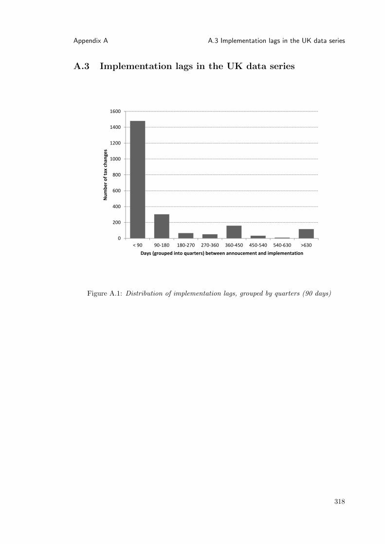
Appendix A A.3 Implementation lags in the UK data series
A.3 Implementation lags in the UK data series
0
200
400
600
800
1000
1200
1400
1600
< 90 90-180 180-270 270-360 360-450 450-540 540-630 >630
Nu
mb
er
of
tax
ch
an
ge
s
Days (grouped into quarters) between annoucement and implementation
Figure A.1: Distribution of implementation lags, grouped by quarters (90 days)
318
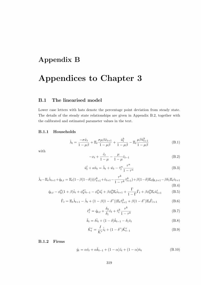
Appendix B
Appendices to Chapter 3
B.1 The linearised model
Lower case letters with hats denote the percentage point deviation from steady state.
The details of the steady state relationships are given in Appendix B.2, together with
the calibrated and estimated parameter values in the text.
B.1.1 Households
λt =−σxt
1− µβ+ Et
σµβxt+1
1− µβ+
ubt1− µβ
− Etµβubt+1
1− µβ(B.1)
with
−xt +ct
1− µ− µ
1− µct−1 (B.2)
ult + κnt = λt + wt − τntτn
1− τn(B.3)
λt−Etλt+1+qk,t = Et(1−β(1−δ))(rkt+1+vt+1−τk
1− τkτkt+1)+β(1−δ)Etqk,t+1−βδ1Etvt+1
(B.4)
qk,t − φ′′k(1 + β)it + φ′′k it−1 − φ′′kuit + βφ′′kEtit+1 +Γ
1− ΓΓt + βφ′′kEtuit+1 (B.5)
Γt = Etλt+1 − λt + (1− β(1− δτ ))Etτkt+1 + β(1− δτ )EtΓt+1 (B.6)
rkt = qk,t +δ2
δ1vt + τkt
τk
1− τk(B.7)
kt = δit + (1− δ)kt−1 − δ1vt (B.8)
Kτt =I
Kτit + (1− δτ )Kτt−1 (B.9)
B.1.2 Firms
yt = αvt + αkt−1 + (1− α)zt + (1− α)nt (B.10)
319
Appendix B B.1 The linearised model
wt = mct + yt − nt (B.11)
rkt = mct + yt − kt−1 − vt (B.12)
πt = Etπt+1 +(1− η)(1− βη)
ηmct (B.13)
B.1.3 Market clearing
yt =C
Yct +
I
Yit +
G
Ygt (B.14)
B.1.4 Policy
Dividing equations (3.38) and (3.39) by Yt, linearizing and defining RN,Xt = RN,Xt − ytyields:
∆RNt =wNTNn /Y
RN(∆wt−1 + ∆nt−1 + ∆TNn,t −∆yt)
+rkKTNk /Y
RN(∆rkt−1 + ∆vt−1 + ∆Kt−2 −∆yt) +
rkKTNk /Y − δτK/YRN
∆TNk,t
− (δτK/YRN
)(∆Kt−2 −∆yt)
(B.15)
and
∆RXt =wNTXn /Y
RX(∆wt−1 + ∆nt−1 + ∆TXn,t −∆yt)
+rkKTXk /Y
RX(∆rkt−1 + ∆vt−1 + ∆Kt−2 −∆yt) +
rkKTXk /Y − δτK/YRX
∆TXk,t
− (δτK/YRX
)(∆Kt−2 −∆yt).
(B.16)
The ∆Rt terms reflect the change in the percentage deviation from steady state. Multi-
plying this by the steady state revenue-to-GDP ratio R would then give the percentage
point change in the revenue-to-GDP ratio. This would be equivalent to the narrative
shocks. Therefore, define the model-equivalent narrative variable as εN,X , and θN,X as
the steady state ratio, which then implies:
εNt = θN∆RNt (B.17)
εXt = θX∆RXt . (B.18)
These two variables are related to the data via the measurement equations in Chapter 3.
Movements in the model’s tax rates are governed by endogenous and exogenous move-
320
Appendix B B.2 The steady state
ments, as discussed in Chapter 3. This means that the linearised tax rules are:
Υnt = γny yt + γnb bt−1 + γng gt + νnt (B.19)
Υkt = γky yt + γkb bt−1 + γkg gt + νkt (B.20)
τnt = Υnt + xnt (B.21)
and
τkt = Υkt + xkt (B.22)
with xt an exogenous AR(1) process. Government spending and transfers are described
as follows:
gt = −γgy yt − γgb bt−1 + ugt (B.23)
LSt = −γLSy yt − γLSb bt−1 + uLSt . (B.24)
The government budget constraint is given by:
Bbt − (B/β)bt−1 − (B/β)rt−1 =τk(MCαY − δτK)τkt − τkδτKKτt−1 + τkMCαY (yt + mct)
+ τnMC(1− α)Y (τnt + yt + mct)
(B.25)
Monetary policy is described by the interest rate rule:
Rt = ψRRt−1 + (1− ψR)(ψππt + ψyyt) + eRt . (B.26)
B.2 The steady state
I = δK (B.27)
MC =ε− 1
ε(B.28)
Kτ =Λ
δττk=
I
δτ(B.29)
Γ =βδττk
(1− β(1− δτ ))(B.30)
K
Y=β(1− τk)αMC
(1− β(1− δ))(B.31)
Y =
(K
Y
) α1−α
N (B.32)
δ1 =(1− τk)α
K(B.33)
321

Appendix B B.3 Chapter 3 Data Appendix
R = (1− α)MCτnY + τk(MCαY − δτK) (B.34)
B.3 Chapter 3 Data Appendix
Table (B.1) describes the data construction. The data largely come from the Bureau of
Economic Analysis’ NIPA tables, downloaded on 17th May 2011. The nominal variables
are converted into real variables using the GDP deflator for personal consumption expen-
ditures (NIPA Table 1.1.4, line 2). The data are transformed into per capita variables
by dividing through by the total civilian noninstitutional population from the Federal
Reserve Bank of St. Louis Federal Reserve Economic Data (FRED), originally from the
Bureau of Labor Statistics (BLS). Variables are then converted into logs and multiplied
by 100. Variables in bold are used in the estimation.
322

Appendix B B.3 Chapter 3 Data Appendix
Table B.1: Chapter 3 Data SourcesSeries Source Construction
Consumption BEA Personal consumption expenditures on nondurable goods (Table1.1.5 line 4) plus services (Table 1.1.5 line 5).
Investment BEA Gross private domestic investment (Table 1.1.5 line 7) plusdurable goods (Table 1.1.5 line 4).
Average personal taxrate
BEA τp = PW+PRI/2+CI
where P is personal current taxes (Table 3.2
line 3), W is wage and salary accruals (Table 1.1.12 line 3), PRIis proprietors’ income (Table 1.1.12 line 9), CI is capital income,defined as rental income (Table 1.1.12 line 12), corporate profits(Table 1.1.12 line 13) and net interest (Table 1.1.12 line 18) andPRI/2.
Labour tax rate BEA τn = τp(W+PRI/2)+CSIEC+PRI/2
where CSI is contributions for govern-
ment social insurance (Table 3.2 line 11) and EC is compensa-tion of employees (Table 1.1.12 line 2).
Capital tax rate BEA τk = τpCI+CTCI+PT
where CT is tax on corporate income (Table 3.2line 8) and PT are property taxes (Table 3.3, line 8).
Labour tax rev-enues
BEA τn × (EC + PRI/2).
Capital tax rev-enues
BEA τk × (CI + PT ).
Governmentspending
BEA Consumption expenditures (Table 3.2 line 21) plus gross govern-ment investment (Table 3.2 line 32), net purchases of nonpro-duced assets (Table 3.2 line 44) less consumption of fixed capital(Table 3.2 line 45).
Transfers BEA Current transfer payments (Table 3.2 line 22) minus currenttransfer receipts (Table 3.2, line 16); plus capital transfer pay-ments (Table 3.2 line 43) minus capital transfer receipts (Table3.2 line 39); minus current tax receipts (Table 3.2 line 2), con-tributions for government social insurance (Table 3.2 line 11),income receipts on assets (Table 3.2 line 12), current surpluson government enterprises (Table 3.2 line 19) plus capital andlabour tax revenue (defined above).
Government debt BEA Bt = NB − (Mt −Mt−1) + Bt−1 where Mt −Mt−1 is the ad-justed monetary base (St. Louis Fed series AMBSL). NB is netborrowing as defined in the NIPA.
Hours BLS Nonfarm business average weekly hours index (2005=100). BLSseries PRS85006023.
Employment FRED Civilian employment, FRED/BLS series CE16OV.
Hours worked N = Hours×Employment100
.
Population index FRED/BLS Civilian noninstitutional population, 16 years and older. FREDseries CNP16OV/BLS series LNS10000000.
Inflation BEA First difference of the (log) GDP deflator (Table 1.1.4 line 1).
Nominal interestrate
St Louis Fed Effective Federal Funds Rate (FEDFUNDS), averaged to yielda quarterly series, expressed at a quarterly rate.
Endogenous taxchanges
Romer andRomer (2010)
Sum of spending-driven, countercyclical and deficit-driven taxchanges.
Exogenous taxchanges
Romer andRomer (2010)
Long-run tax changes.
323

Appendix C
Appendices to Chapter 4
C.1 Chapter 4 Data Appendix
The data span the period 1955:1 to 2007:4. Real government spending, real consumption,
real investment and real GDP come directly from the Bureau of Economic Analysis NIPA
tables. All variables are the log of real per capita variables. Nominal variables are
deflated by their own implicit price deflators with the exception of government spending
which is deflated by the GDP deflator. Real hours are an unpublished Bureau of Labor
Statistics (BLS) series, downloadable from Valerie Ramey’s website. The real wage is
real hourly compensation, non-farm business, in logs from the BLS. Population is total
civilian population also from the BLS. Table (C.1) contains a summary of the data.
Real per capita debt is the log of my constructed debt measure divided by the total
population and the GDP deflator. The debt measure is very close the ‘Debt Held by the
Public’. This series is only available from 1970, so I construct a proxy from old editions
of the United States Treasury Bulletin back to 1947. For the pre-1974 period this is the
‘Total Public Issues’ series. After 1974, for consistency, I have to construct the ‘Total
Public Issues’ series from the Monthly Statement of Public Debt by combining ‘Total
Interest Bearing Debt’ minus the ‘Government Accounts Series’ plus ‘Total Treasury
Deposit Funds’. Because this is not an exact match to ‘Debt Held by the Public’ I check
how close the two measures are (for the common part of the series, 1970 onwards) —
the R squared is 0.999, so I am confident that my constructed series reflects changes in
‘Debt Held By the Public’.
The capital and labour income tax rates are constructed following Jones (2002). I
reconstruct the series, extend it back to 1947 following Burnside et al. (2004) and forward
to 2008. As a check, I reproduce the narrative Vector Autoregression results in Burnside
et al. (2004), the results are very similar. These extra results are available on request.
324

Appendix C C.2 Linearised model
Table C.1: Chapter 4 Data sources
Series Source Description
Gov. spending BEA Gov. cons. expenditures and gross inv. (CVM)
Capital taxes BEA Constructed as above
Labour taxes BEA Constructed as above
Output BEA Gross domestic product (CVM)
Real wage BLS BLS Series ID: PRS85006153
Hours Unpublished BLS Francis-Ramey “Measures of Hours per Capita”
Consumption BEA Personal consumption expenditures (CVM)
Investment BEA Gross private domestic investment (CVM)
Debt Treasury Bulletin Close to ‘Debt Held by the Public’
C.2 Linearised model
C.2.1 Notation
Lower case letters represent the percentage deviation of each variable from its steady
state value. The only exceptions are the tax rates τNt and τKt which are expressed as
percentage point deviations to match the variable definition in the VAR.
C.2.2 Households
a1ct + a2nt + a3xt + a4xt−1 + a5µt − a6λt + a7ct−1 = 0 (C.1)
λt + wt −1
1− τNτNt = b1ct + b2nt + b3xt + b4ct−1 (C.2)
c1ct + c2nt + c3xt + c6ct−1 + µµt = c4µt+1 + c5ct+1 (C.3)
Etλt+1 = λt − rt (C.4)
(1− h)xt = (1− h)(1− γ)xt−1 + γct − hγct−1 (C.5)
ωqt − (1 + β)it + it−1 − βEtit+1 = 0 (C.6)
where ω = 1φ′′ .
qt + rt = rK(1− τK)βEtrKt+1 − βrKEtτKt+1 + β(1− δ)Etqt+1 − βδ′(z)zEtzt+1 (C.7)
where the coefficients are given at the end of this appendix.
C.2.3 Firms
Up to a first order approximation the aggregate production function is given by
yt = αzt + αkt + (1− α)nt (C.8)
325

Appendix C C.2 Linearised model
and factors are paid
rKt = mct + yt − kt (C.9)
wt = mct + yt − nt. (C.10)
Utilisation is described by
(1 + κ)zt = yt − kt − qt +mct −1
1− τKτKt (C.11)
where κ = δ′′
δ′ .
Price evolution is determined by the New Keynesian Phillips Curve
πt = βEtπt+1 +(1− η)(1− βη)
ηmct. (C.12)
C.2.4 Policy rules
rt − Etπt+1 = φππt (C.13)
τnt = θgngt + θn1τnt−1 + θn2τnt−2 (C.14)
τkt = θgkgt + θk1τkt−1 + θk2τnt−2 (C.15)
gt = φ1gt−1 + φ2at (C.16)
T
YTt =
B
Y
1
R(bt+1−rt)−
B
Ybt =
G
Ygt−(1−α)τn(τnt +nt+wt)−ατk(τkt +rkt +kt). (C.17)
C.2.5 Identities
δit = kt+1 − (1− δ)kt (C.18)
yt =C
Yct +
I
Yit +
G
Ygt. (C.19)
C.2.6 Stochastic processes
at+1 = ρat + εt+1 (C.20)
The 3 predetermined variables are:
{bt, kt, at}
and the control variables are:
{ct, πt, wt, nt, xt, yt, rkt ,mct, qt, zt, λt, µt, rt, τKt , τNt , gt, it}
326
Appendix C C.3 The steady state
C.2.7 Coefficients from the linearised Jaimovich–Rebelo preferences
a1 = (γ − 1)µγX1−γ(C(1− h))γ−2C − σCχ(C − hC − ψN ξX)−1
a2 = ξψN ξXσ(C − hC − ψN ξX)−σ−1
a3 = ψN ξXσ(C − hC − ψN ξX)−σ−1
a4 = (1− γ)µγX1−γ(C(1− h))γ−1
a5 = µγX1−γ(C(1− h))γ−1
a6 = µγX1−γ(C(1− h))γ−1 + χ
a7 = −ha1
b1 = −(σψN ξ−ξX((C − hC − ψN ξX)−σ−1)C)/(a6W (1− τN ))
b2 = ((ξ − 1)ψXN ξ−1ξχ+ σψ2N2ξ−1ξ2X2(C − hC − ψN ξX)−σ−1)/(a6W (1− τN ))
b3 = X(ψN ξ−1ξχ+ ψN ξ−1ξX(σ((C − hC − ψN ξX)−σ−1)ψN ξ))/(a6W (1− τN ))
b4 = −hb1
c1 = −σψN ξ(C − hC − ψN ξX)−σ−1C + h(1− γ)µβγ(C(1− h))γ−1X−γC
c2 = ψ2ξXσN2ξ(C − hC − ψN ξX)−σ−1 + ξψN ξχ
c3 = σψ2N2ξ(C − hC − ψN ξX)−σ−1X + γµβ(1− γ)(C(1− h))γX−γ
c4 = µβ(1− γ)(C(1− h))γX−γ
c5 = γµβ(1− γ)(C(1− h))γ−1X−γC
c6 = σhψN ξ(C − hC − ψN ξX)−σ−1C
χ = (C − hC − ψN ξX)−σ
C.3 The steady state
Our assumptions of φ(I/K) imply that
I
K= δ
327

Appendix C C.3 The steady state
thereforeI
Y=
I
K
K
Y= δ
K
Y.
Given the tax and subsidy on revenue (mc = 1), the state version of the return on capital
implies
rK = αY
K.
From equation (4.14)
rK =R− 1 + δ
1− τK(C.21)
thereforeK
Y=
α
rK(C.22)
andI
Y=δα
rK. (C.23)
The share of consumption can be written
C
Y= 1− δK
Y− G
Y, (C.24)
This follows from the resource constraint, equation (4.23).
ψ can be found by solving the household’s steady state first order conditions
ψ =
(N ξ
[ξX
W (1− τN )N− γX1−γ(C(1− h))γ−1
β(1− γ)(C(1− h))γX−γ − 1
])−1
(C.25)
where N is steady state hours and is calibrated.
From the production function and the marginal product of capital is
K =
(rK
α
)( 1α−1)
N (C.26)
and dividing the resource constraint by K gives an expression for CK. Using this together
with equation (C.26) yields an expression for steady state consumption. The steady state
real wage follows from
W = (1− α)
(K
N
)α. (C.27)
µ is the steady state Lagrange multiplier
µ =ψN ξχ
β(1− γ)(C(1− h))γX−γ − 1. (C.28)
From equation (4.8), steady state X is given by:
X = C(1− h). (C.29)
328

Appendix C C.3 The steady state
The steady state gross real interest rate is related to the discount factor
R =1
β. (C.30)
From the first order condition for zt
δ′(z)z = (1− τK)αY
K. (C.31)
BY is calibrated.
329

Bibliography
Adam, S., Browne, J., and Heady, C. (2010). “Taxation in the U.K.” in Dimensions of
Tax Design: The Mirrlees Review. Oxford University Press.
Alesina, A., Ardagna, S., Perotti, R., and Schiantarelli, F. (2002). “Fiscal policy, profits
and investment.” American Economic Review, 92(3), 571–589.
Altig, D., Christiano, L., Eichenbaum, M., and Linde, J. (2005). “Firm-specific capital,
nominal rigidities and the business cycle.” NBER Working Paper No.11034.
Auerbach, A. (1989). “Tax reform and adjustment costs: the impact on investment and
market value.” International Economics Review, 30(4), 939–962.
Baxter, M., and King, R. (1993). “Fiscal policy in general equilibrium.” American Eco-
nomic Review, 83, 315–334.
Beetsma, R. (2008). “A survey of the effects of discretionary fiscal policy.” Working
Paper, University of Amsterdam.
Benhabib, J., Schmitt-Grohe, S., and Uribe, M. (2001). “Monetary Policy and Multiple
Equilibria.” American Economic Review, 90, 40–69.
Blanchard, O., and Perotti, R. (2002). “An empirical characterization of the dynamic
effects of changes in government spending and taxes on output.” Quarterly Journal of
Economics, 117, 1329–1368.
Blow, L., and Preston, I. (2002). “Deadweight loss and taxation of earned income: evi-
dence from tax records of the UK self employed.” Institute for Fiscal Studies Working
Paper WP02/15.
Blundell, R., Brewer, M., and Shephard, A. (2005). “Evaluating the labour market impact
of Working Families’ Tax Credit using differences-in-differences.” HM Revenue and
Customs Working Paper 4.
Blundell, R., Duncan, A., and Meghir, C. (1998). “Estimating labor supply responses
using tax reforms.” Econometrica, 66(4), 827–861.
330

BIBLIOGRAPHY
Britton, A. (1991). Macroeconomic policy in Britain 1974-87. Cambridge University
Press.
Burnside, C., Eichenbaum, M., and Fisher, J. D. (2004). “Fiscal shocks and their conse-
quences.” Journal of Economic Theory, 115, 89–117.
Cairncross, A. (1992). The British economy since 1945. Blackwell publishers.
Calvo, C. A. (1983). “Staggered prices in a utility maximizing framework.” Journal of
Monetary Economics, 12(3), 983–998.
Canova, F. (2007). Methods for Applied Macroeconomic Research. Princeton University
Press.
Christiano, L., Eichenbaum, M., and Evans, C. (1996). “The effects of monetary policy
shocks: evidence from the flow of funds.” Review of Economics and Statistics, 78(1),
16–34.
Christiano, L., Eichenbaum, M., and Evans, C. (2005). “Nominal rigidities and the dy-
namic effects of a shock to monetary policy.” Journal of Political Economy, 113, No.1.
Coenen, G., and Straub, R. (2005). “Non-Ricardian Households and fiscal policy in an
estimated DSGE model of the Euro Area.” In: Computing in Economics and Finance,
102.
Cogan, J., Cwik, T., Taylor, J., and Wieland, V. (2010). “New Keynesian versus Old Key-
nesian government spending multipliers.” Journal of Economic Dynamics and Control,
34(3), 281–295.
Cummins, J., Hassett, K., and Hubbard, R. (1996). “Tax reforms and investment: A
cross-country comparison.” Journal of Public Economics, 62 (1-2), 237 – 273.
Davig, T., and Leeper, E. (2006). “Fluctuating macro policies and the fiscal theory.” In:
NBER Macroeconomics Annual 2006, 247–298.
Davig, T., and Leeper, E. (2011). “Monetary-fiscal policy interactions and fiscal stimu-
lus.” European Economic Review, 55(2), 211–227.
Dow, C. (1964). The management of the British economy 1945-60. The Syndics of the
Cambridge University Press.
Dow, C. (2000). Major Recessions: Britain and the World, 1920-1995. Oxford University
Press.
Favero, C., and Giavazzi, F. (2007). “Debt and the effects of fiscal policy.” NBER Working
Paper No. 12822.
331

BIBLIOGRAPHY
Favero, C., and Giavazzi, F. (2010). “Reconciling VAR-based and narrative measures of
the tax multiplier.” American Economic Journal: Economic Policy, Forthcoming.
Forni, L., Monteforte, L., and Sessa, L. (2009). “The general equilibrium effects of fiscal
policy: Estimates for the Euro Area.” Journal of Public Economics, 93(3-4), 559–585.
Gali, J. (2008). Monetary Policy, Inflation, and the Business Cycle. Princeton University
Press.
Geweke, J. (1999). “Using simulation methods for Bayesian econometric models: Infer-
ence, development and communication.” Econometric Reviews, 18(1), 1–73.
Greenwood, J., Hercowitz, Z., and Huffman, G. (1988). “Investment, capacity utilization,
and real business cycles.” American Economic Review, 78, 402–417.
Gregg, P., and Harkness, S. (2003). “Welfare reform and lone parents employment in the
UK.” Centre for Market and Public Organisation Working Paper, 03/072.
Hall, A., Inoue, A., Nason M, J., and Rossi, B. (2010). “Information criteria for impulse
response function matching estimation of DSGE models.” Duke University Working
Papers 10-28.
Jaimovich, N., and Rebelo, S. (2009). “Can news about the future drive the business
cyle?” American Economic Review, 99(4), 1097–1118.
Jones, J. (2002). “Has fiscal policy helped stabilize the postwar U.S. economy?” Journal
of Monetary Economics, 49, 709–746.
King, R., Plosser, C., and Rebelo, S. (1988). “Production, growth and business cycles I.
The basic neoclassical model.” Journal of Monetary Economics, 21, 195–232.
King, R., and Rebelo, S. (1999). “Resurrecting real business cycles.” Handbook of Macroe-
conomics, Volume 1, 927–1007.
Klein, P. (2000). “Using the Generalized Schur form to solve a multivariate linear rational
expectations model.” Journal of Economic Dynamics and Control, 24(10), 1405–1423.
Leeper, E. (1991). “Equilibria under ‘active’ and ‘passive’ monetary and fiscal policy.”
Journal of Monetary Economics, 27, 129–147.
Leeper, E., Plante, M., and Traum, N. (2010). “Dynamics of fiscal financing in the United
States.” Journal of Econometrics, 156, 304–321.
Linnemann, L. (2006). “The effect of government spending on private consumption: A
puzzle?” Journal of Money, Credit and Banking, 38(7), 1715–1735.
332

BIBLIOGRAPHY
Lopez-Salido, J., and Rabanal, P. (2008). “Government spending and consumption-hours
preferences.” Manuscript, Federal Reserve Board.
McGrattan, E. R. (1994). “The macroeconomic effects of distortionary taxation.” Journal
of Monetary Economics, 33, 573–601.
Mertens, K., and Ravn, M. (2010). “Empirical evidence on the aggregate effects of an-
ticipated and unanticipated U.S. tax policy shocks.” NBER Working Paper 16289.
Mertens, K., and Ravn, M. O. (2011a). “Measuring fiscal shocks in Structural VARs
using narrative data.” Manuscript, Cornell University and University College London.
Mertens, K., and Ravn, M. O. (2011b). “Understanding the aggregate effects of antic-
ipated and unanticipated tax policy shocks.” Review of Economic Dynamics, 14(1),
27–54.
Monacelli, T., and Perotti, R. (2009). “Fiscal policy, wealth effects, and markups.” CEPR
Discussion Paper DP7099.
Perotti, R. (2005). “Estimating the effects of fiscal policy in OECD countries.” CEPR
Discussion Paper No. 4842.
Perotti, R. (2007). “In search of the transmission mechanism of fiscal policy.” NBER
Working Paper, 13143.
Perotti, R. (2010). “The effects of tax shocks on output: not so large, but not small
either.” NBER Working Paper No. 16786.
Ramey, V., and Shapiro, M. (1998). “Costly capital reallocation and the effects of govern-
ment spending.” Carnegie Rochester Conference Series on Public Policy, 48, 145–194.
Ramey, V. A. (2011). “Identifying government spending shocks: It’s all in the timing.”
Quarterly Journal of Economics, 126(1), 1–50.
Ratto, M., Werner, R., and in ’t Veld, J. (2009). “Fiscal policy in an estimated open-
economy model for the Euro Area.” Economic Modelling, 26(1), 222–233.
Ravn, M. O., Schmitt-Grohe, S., and Uribe, M. (2006). “Deep Habits.” Review of Eco-
nomic Studies, 73(1), 195–218.
Ravn, M. O., Schmitt-Grohe, S., and Uribe, M. (2007). “Explaining the effects of govern-
ment spending shocks on consumption and the real exchange rate.” NBER Working
Paper, 13328.
Reis, R. (2008). “Using VARs to identify models of fiscal policy: A comment on Perotti.”
NBER Macroeconomics Annual 2007, 22.
333

BIBLIOGRAPHY
Romer, C., and Romer, D. (1989). “Does monetary policy matter? A new test in the
spirit of Friedman and Schwartz.” In NBER Macroeconomic Annual 1989.
Romer, C., and Romer, D. (2004). “A new measure of monetary shocks: Derivation and
implications.” American Economic Review, 94(4), 1055–84.
Romer, C., and Romer, D. (2009a). “Do tax cuts strave the beast? the effect of tax
changes on government spending.” Brookings Papers on Economic Activity, Spring,
139–200.
Romer, C., and Romer, D. (2009b). “A narrative analysis of postwar tax changes.”
Manuscript, University of California, Berkeley.
Romer, C., and Romer, D. (2010). “The macroeconomic effects of tax changes: Estimates
based on a new measure of fiscal shocks.” American Economic Review, 100(June), 763–
801.
Schmitt-Grohe, S., and Uribe, M. (2010). “What’s ‘news’ in business cycles.” mimeo,
Columbia University.
Smets, F., and Wouters, R. (2003). “An estimated dynamic stochastic general equilibrium
model of the Euro Area.” Journal of the European Economic Association, 1(5), 1123–
1175.
Smets, F., and Wouters, R. (2007). “Shocks and frictions in US business cycles: a
Bayesian DSGE approach.” American Economic Review, 97(3), 586–606.
Traum, N., and Yang, S.-C. (2009). “When does government debt crowd out investment?”
Manuscript, Indiana University.
Traum, N., and Yang, S.-C. (2010). “Monetary and Fiscal Policy Interactions in the
Post-war U.S.” IMF Working Paper, November 2010.
Woodford, M. (2003). Interest and Prices: Foundations of a Theory of Monetary Policy.
Princeton University Press.
Woodward, N. (2004). The management of the British economy, 1945-2001. Manchester
University Press.
Zubairy, S. (2009). “Explaining the effects of government spending shocks.” Mimeo, Duke
University.
Zubairy, S. (2010). “On fiscal multipliers: Estimates from a medium scale DSGE model.”
Bank of Canada Working Paper 2010-30.
334
Recommended