The Parking Lot Problem
Maria Arbatskaya, Kaushik Mukhopadhaya, and Eric Rasmusen
July 22, 2004
Abstract
If there is competition for access to an underpriced good such as a free parking spot,the competition can eat up the entire surplus, eliminating the social value of the good.There is a discontinuity in social welfare between “enough” and “not enough,” with theminimum social welfare being at slightly too small a parking lot because of the rent-seeking efforts of drivers. Uncertainty over the number of drivers actually increasessocial welfare if the parking lot size is set too small; if it is set optimally, the parkinglot size will be well in excess of mean demand.
Keywords: rent-seeking, all-pay auction, timing, capacity size, queue.JEL classification numbers: R4; L91; D72.
Maria Arbatskaya, Department of Economics, Emory University, Atlanta, GA 30322-2240. Phone: (404) 727 2770. Fax: (404) 727 4639. Email: [email protected].
Kaushik Mukhopadhaya, 194 Ivy Glen Circle, Avondale Estates, GA 30002. Phone:(404) 292 9491.
Eric Rasmusen, Indiana University Foundation Professor, Department of Business Eco-nomics and Public Policy, Kelley School of Business, Indiana University, BU 456, 1309E 10th Street, Bloomington, Indiana, 47405-1701. Phone: (812) 855 9219. Fax: (812)855 3354. Email: [email protected]. http://www.rasmusen.org.
AcknowledgmentsWe would like to thank Michael Alexeev, Theodore Bergstrom, Robert Deacon, DanielKovenock, John Lott, Milton Kafoglis, and seminar participants at Purdue University,Virginia Polytechnic Institute, the 2001 Public Choice Meetings, the 2003 EconometricSociety Summer Meetings, and the 2004 World Congress of the Game Theory Societyfor helpful comments. Rasmusen thanks Harvard Law School’s Olin Center and theUniversity of Tokyo’s Center for International Research on the Japanese Economy fortheir hospitality while this paper was being written. Copies of this paper can be foundat http://www.rasmusen.org/papers/parking- rasmusen.pdf.

1. Introduction
Finding a parking space is a perennial source of frustration. College campuses are especially
prone to parking shortages. Tough competition between students for a limited number of
parking spaces compels students to arrive well in advance their preferred time. The October
15, 1994 Los Angeles Times reports that in one California college, a parking permit is no
more than a hunting license. “Survival of the earliest” is the rule, and students arrive hours
in advance to find a parking spot. On the other hand, shopping malls display an apparently
useless excess of parking spaces. In contrast to such public institutions as state universities
and downtown retailing districts, which have too little parking, malls seem to go to ridiculous
extremes with their acres of parking lots which are never full except around Christmas.
Parking studies recognize the importance of planning for a sufficient ‘cushion’ in ex-
cess of the necessary spaces. However, these studies are mostly concerned with the smooth
flow of vehicles in and out of the parking area and unforeseen circumstances such as mi-
nor construction. The 1987 study by Walker Parking Consultants (commissioned by In-
dianapolis to develop a Regional Center Parking Plan) says, “Thus, a supply of parking
operates at peak efficiency when occupancy is 85% to 90%. When occupancy exceeds
this level, there may be delays and frustration in finding a space. The parking supply
may be perceived as inadequate even though there are spaces available in the system”
(http://www.bts.gov/NTL/DOCS/rc.html). We suggest that an equally important concern
is strategic behavior by drivers. If the parking lot is built just slightly too small, rent-seeking
competition can dissipate all of the rents from parking there, eliminating every trace of the
lot’s social usefulness and making its construction cost entirely wasteful. Hence, more impor-
tant than any engineering concern is that a parking lot should be sufficiently large to avoid
wasteful competition for parking spaces. It can easily be socially optimal to have parking
lots that on average are half empty, as we will show below by example. Shopping malls seem
to realize this better than public or nonprofit institutions.
It is natural to view empty spaces as a reason to reduce the amount of parking. Based
on the finding that the average parking supply count exceeded demand count by 30%, for
example, a Seattle report recommends reducing the parking supply there. The authors
2

admit, however, that “A major policy-related issue is how much allowance to provide over
the design-level demand in setting the size of a given parking facility.”1
We believe that strategic behavior must be considered when deciding on parking lot
size. Having 30% of the spaces empty may well indicate too small a parking lot size, given
uncertainty in the demand for parking. We will show that there is a strategic asymmetry in
the welfare effects of over- and under-supply of parking. Extra parking spaces are costly in
proportion to their number, but even a small shortage in parking can result in a discontinuous
and huge social loss, and the welfare loss can be higher at a small shortage than at a large
shortage.
We thus construct a model of competition between drivers for parking spaces. The drivers
face a trade-off between the disutility of arriving earlier than their preferred time and the
increased probability of securing a space in the parking lot. Since the cost of arriving early
is incurred regardless of whether a driver is successful in finding a parking space, the contest
is a multi-unit all-pay auction. Due to the dynamic nature of the players’ decisions on when
to arrive at the lot, their strategies can be quite complex. Nevertheless, we are able to show
that full (or almost full) rent dissipation occurs whenever the size of the lot is too small.
The model describes a dynamic competition for a given supply of goods. The trade-off
between arriving later and reducing one’s chances of obtaining a good is by no means limited
to the parking problem. The trade-off can arise in a number of diverse applications. People in
need of vaccination may try to overcome vaccine shortages by demanding the vaccine earlier,
when there is still uncertainty about the severity and features of the next virus outbreak.
Parents may sign up their kids to a daycare just to keep the spot to themselves when they
really need it. Firms may preempt other firms by approaching potential acquisition targets
before other firms. Bargain hunters may have to arrive earlier to ensure the availability of
a product at a bargain price. People who have relatives living in different time zones may
start calling their relatives ahead of their preferred time (at midnight of the New Year Eve)
for fear of not being able to get through later.
Section 2 of the paper will provide a brief discussion of the literature on the subject.
In Section 3, we describe parking as a dynamic discrete-time competition between a known
1See the 1991 Parking Utilization Study undertaken by the Research and Market Strategy Division of theTransit Department in the Municipality of Metropolitan Seattle.
3

number of drivers for a limited number of parking spaces. We derive pure-strategy subgame-
perfect equilibria under full observability of the parking lot, and show that such equilibria
do not exist under unobservability. Section 4 establishes the full rent dissipation result for
any subgame-perfect equilibria of the parking game. In Section 5, the optimal capacity is
determined for a certain and uncertain number of drivers. We show that in the case of a
known number of drivers, the optimal size of the parking lot is equal to the number of drivers.
When the size of the parking lot is set before the uncertainty about the number of drivers is
resolved and the planners only know its distribution, they should build a sufficiently large
parking lot. On average, a large proportion of the parking spots will be unoccupied for a
parking lot of an optimal size. Section 6 discusses the results and extensions of the model,
and Section 7 concludes.
2. The Literature
The problem of managing a transportation system has been analyzed by urban economists
and operations researchers. Queueing models with tolls, e.g. Naor (1969), assume an exoge-
nous stationary customer arrival process and random service times. Customers benefit from
the service, but have to incur a constant cost per unit of time from queueing. In an equilib-
rium, a consumer joins a queue if its length is below a threshold level. The last consumer
in the queue is just indifferent between joining and staying out. The equilibrium outcome is
inefficient, due to the negative externality that a customer imposes on those arriving later.
Nevertheless, rent dissipation through queueing is not full due to the randomness in the
arrival and departure processes.
Richard Arnott et al. (1993) compare alternative toll regimes in a model with a sin-
gle traffic bottleneck and identical commuters incurring linear time inconvenience cost (the
“schedule delay cost”). Recent papers by Anderson and de Palma (2004) and Arnott and
John Rowse (1999) study pricing of parking. Richard Porter (1977), writes on the optimal
size of underpriced facilities, and points out that congestion is better than queuing, but does
not seem to note the discontinuity, or actually solve for the optimal size.
The strategic incentives of people to adjust their purchase schedules are analyzed by
4

Robert Deacon and Jon Sonstelie (1991). Consumers choose the size of purchases to minimize
the total cost of shopping for an underpriced good, which includes shopping and storage
costs. The waiting time in a queue increases until the market clears. The authors note
that consumers are no better off from a price ceiling, though suppliers are worse off, thus
generating a deadweight loss in rationing by waiting. (See also Deacon & Sonstelie [1985,
1989] and Deacon [1994].)
Other economists have looked at similar problems; notably, William Vickrey, more fa-
mous for his work on auction theory. In “pure bottleneck” congestion in transportation
facilities, queues form at a single route segment of fixed capacity. In Vickrey’s 1969 pure
bottleneck model, commuters have preferred travel times through the bottleneck, distributed
uniformly. For a sufficiently large capacity, no queue develops and the commuters arrive at
their preferred times. For a smaller capacity, this is not possible, a queue develops and some
commuters arrive early or late. Each commuter faces a trade-off between the disutility of
arriving at a less-preferred time and the cost of waiting in line. Vickrey notes a “sharp
discontinuity” in the amount of delay at the level of capacity just sufficient to accommo-
date the traffic, and points out that optimal investments in capacity extension differ in the
first-best and the second-best situations. In the first-best, using the optimal price structure
(a toll fee that leads to efficient facility use), the benefits of capacity extension are not as
“capricious” as in the second-best, when access cannot be restricted by fees. In the second-
best, “Expansion inadequate to take care of the entire traffic demand...may turn out to be
hardly worthwhile...” In Vickrey’s model, however, capacity extension reduces delays and is
beneficial to travellers. We will show that an insufficient increase in capacity might not have
any benefit whatsoever to offset construction costs, so that the facility is a pure waste.
The idea closest to that modelled in the present paper is Steven Landsburg aquarium
story in The Armchair Economist, in which all gains from a facility with free access are
dissipated by congestion. Building a new aquarium does not benefit anyone while it is costly
to build. In a way, the result is similar to the zero-profit outcome in a contestable market:
potential competition (here by consumers) puts pressure on the active competitors. At the
margin, the players’ surplus is zero, and a given player is indifferent between using and not
using the facility.
5

In the theory of waiting lists proposed by Lindsay and Feigenbaum (1984), market clearing
occurs due to depreciation of product value in time. Since delivery of a service in future
can be less valuable than immediate delivery, potential consumers are discouraged from
putting their names on the list when it is too long. By this argument the authors explain
the persistence of long waiting lists for non-emergency in-patient care at Britain’s National
Health Service and the fruitlessness of short-term measures aimed at a substantial reduction
of the waiting list. See, however, the critique by Cullis and Jones ( 1986).
In our model, there are no waiting lists, congestion, or waiting in line. Rather, rent
dissipation comes in the form of costly schedule adjustment by the travellers. In an effort
to secure a parking spot, they come well in advance of their preferred time and dissipate
nearly all rents whenever the number of drivers exceeds the number of parking spaces. The
parking game under unobservability is closely related to all-pay auction models such as those
of Holt and Sherman (1982), Barut and Kovenock (1998), and Clark and Riis (1998). These
papers establish rent dissipation results for multi-prize all-pay auctions in which players
make one-time decisions about their bids chosen from a continuous space.2
In the parking model, bids correspond to the cost of earlier arrival. When the game is
played in time, players can possibly react to earlier moves by other players. Hence, we also
examine the full observability case. Under observability, the mathematical structure of the
parking game is related to preemption games and games of timing such as those of Fudenberg
and Tirole (1985) and Simon and Stinchcombe (1989).
Our results will call to mind “jumping the gun” matching games such as those studied
by Roth & Xing (1994) and Avery et al. (2001). To take the example of Avery et al., federal
judges must each select one clerk from graduating law students, and students can work for
no more than one judge. What has happened in recent years is that clerks and judges pair
up earlier and earlier, rather towards the end of the student’s last year of law school. A
judge who waits too long to hire would not be able to find any good clerks still free, so
2In Holt & Sherman (1982) and Clark & Riis (1998), prizes are equal, but the papers differ in that Holtand Sherman assume incomplete information about players’ valuations while Clark and Riis assume theinformation about asymmetric valuations to be complete. Barut and Kovenock (1998) consider symmetricvaluations and an arbitrary prize structure. Clark and Riis (1998) also study sequential distribution ofprizes, with a number of prizes distributed in each of several rounds. For a general analysis of equilibria insingle-prize all-pay actions with complete information and asymmetric values, see Baye et al. (1996).
6

judges hire clerks early even though much better information is available about an older
student’s quality. The top students are analogous to the parking spaces in our model, and
the possibility of mistakenly hiring an incompetent student is the cost of arriving early.
To sum up, we will describe competition for parking spaces as an all-pay auction because
anyone who shows up early to look for a parking space has borne a cost even if he is
unsuccessful. The auction is a multi-prize auction because there is more than one parking
space. Since bids are reducing over time, the auction is a descending-price (Dutch) auction.
Finally, the auction might be either open-cry or sealed-bid, depending on whether drivers
observe other drivers’ choices or not.
3. The Parking Game
In this section, we introduce the notation, set up the model, and discuss equilibria under
various conditions.
3.1. The Model
A set of players — the drivers — is indexed by I ≡ {1, ..., N}. The drivers are workers who
must show up for work no later than time, t = T . Each driver demands one space in the
parking lot, and his value for it is v > 0, e.g., if he cannot find a spot, he must walk from
somewhere further away at cost v. Let K > 0 be the size of the parking lot. If N ≤ K, then
each driver is guaranteed a parking space, and all drivers choose to arrive at their preferred
time, T . If N > K, however, the drivers compete for spaces, and they may wish to arrive
early to secure a spot.3 Assume that a driver who arrives earlier than time T incurs a cost
of w > 0 per unit of time, so his cost of arrival at time t is L(t) = (T − t)w. We will model
time as discrete, with the interesting case being as the time interval ∆ > 0 shrinks to zero.
Thus, a time grid includes times t = k∆ ∈ [0, T ] where k ∈ {0, ..., T/∆}.
What matters to player i when deciding whether to rush to the parking lot at time t is
the number of parking spaces unoccupied at t and the inconvenience of arrival as early as
t. The history at time t can be summarized by the number of parking spaces, Kt, available.
3Parking competition has a form of first-in/first-out queuing. Other kinds of queues are also possible, ifunobserved in the world. First-in/last-out queues can even lead to social optimality. See Hassin (1985) andits discussion by Nalebuff (1989).
7

We will assume that the size, N , of the parking lot is common knowledge, but it will be
interesting to compare two alternative assumptions on whether a driver knows the number
of spaces still open in the parking lot when he makes his own decision on when to arrive.
We will denote the situation when a player making his arrival decision at time t observes
all arrivals prior to t as full observability, and the situation when he must decide without
knowing if the parking lot is full yet as unobservability.
For any time t, define Nt as the number of unarrived drivers and Kt as the number of
parking spaces still open, soNt = N−K+Kt. At time t, the remaining drivers simultaneously
decide whether to arrive at the parking lot at that instant. Under full observability, the
decision can be conditioned on the number of parking spaces, still available, Kt. Let σi,t ∈
[0, 1] denote the probability that player i arrives at the parking lot at time t. Once a parking
spot is taken by the player, the spot remains occupied until the end of the game. If Player i
arrives at t he obtains a spot with probability pi,t = min {Kt/nt, 1}, where nt ≤ Nt denotes
the number of players arriving at exactly time t.
If Player i arrives at time t, given that Kt ∈ {0, ..., K} parking spaces are unoccupied by
t and nt ∈ {0, ..., Nt} players arrive at t, his payoff is
ui,t = pi,tv − L(t) (1)
A player who arrives at time T and finds no parking space must park in a less convenient
parking lot, obtaining payoff zero. This is the same payoff structure as for an all-pay auc-
tion with multiple prizes. Everyone bids, a bidder pays what he bids, and the prizes are
distributed to the top bidders, with a coin toss breaking ties.
Let us define the indifference arrival time, t∗, as the time at which the arrival cost, L(t∗),
equals the prize value, v. It follows that
t∗ ≡ T − v/w. (2)
A player who arrives at t∗ and finds a parking space receives a payoff of zero since the
disutility of the early arrival equals the value of the parking space. Similarly, define t∗p as the
time at which a player receives a zero payoff from participating in a lottery with probability
p of winning a parking space; t∗p is found from equation pv − L(t∗p) = 0. It follows that
8
t∗p ≡ T − pv/w. (3)
When looking for equilibria, we can restrict our attention to t ≥ t∗ since arriving before
t∗ yields a negative payoff and is strictly dominated by arriving at T . Finally, let t and t
denote the earliest and the latest time any player arrives with a positive probability along
the equilibrium path.
As we are interested in characterizing equilibria which exist for any time grid, even a
very fine one, we will assume that time periods are short.
Definition 1. A time grid is called fine if
∆ <v
(K + 1)w. (4)
When a time grid is fine, there are more than K + 1 periods between t∗ and T since
T − t∗ = v/w > (K + 1)∆. For a fine grid, a player would choose to arrive one period
earlier to increase his odds of getting a parking space. The highest odds of obtaining a
space for integer Kt and Nt are K/(K + 1). Even for these odds, the loss of the one-period
earlier arrival, w∆, is justified by the gain associated with the higher probability of obtaining
parking, (1−K/(K + 1))v. Also note that no more than K players can profitably enter at
time t = t∗ +∆ when the time grid is fine.
3.2. Pure-Strategy Equilibria Under Full Observability
Under full observability, Player i’s strategy specifies the probability of his arrival, σi,t ∈ [0, 1]
at any time t = k∆ ∈ [t∗, T ] and historyKt ∈ {0, ...,K}. In the first best, allN players arrive
at T , and K of them get to park in the parking lot: σi,t = 0 for t < T and σi,T = 1. However,
this cannot be a part of an equilibrium strategy profile when the time grid is fine since each
player would prefer to deviate by arriving just before T and increase his probability of finding
a spot to 100%. We will see that although the details of the equilibrium strategies can
be various and intricate, especially for out-of-equilibrium behavior, the equilibrium payoffs
converge to zero as time becomes closer to continuous: the parking lot will have no benefit
to the drivers.
9

We will start by illustrating the logic of what happens in an alternating equilibrium in the
simplest case of two drivers who compete for one parking space. The pure-strategy arrival
schedule of Claim 1 specifies contingencies under which some players arrive, provided they
have not arrived earlier; under all other contingencies, players do not arrive.
Claim 1. The following are equilibrium strategies under full observability when there are
two drivers and one parking spot (N = 2 and K = 1). Contingent on the parking lot not
being full at time t, (i) at t = t∗ + k∆ ∈ [t∗, t∗1/2) : player 1 arrives if k = 0, 2, 4, ... and
player 2 arrives if k = 1, 3, 5, ...; (ii) at t ∈ [t∗1/2, T ): both players arrive. At t = T : all
players arrive who have not yet arrived.
Proof of Claim 1. To prove that the listed strategies are part of a subgame-perfect Nash
equilibrium we must show that there are no profitable deviations for any player at any point
in time, given the strategy of the opponent.
Both players have equilibrium payoffs of zero. Time t∗ is such that player 1 is indifferent
between arriving at t∗ and not parking in the lot at all. Arriving earlier than t∗ (at t < t∗ )
yields the player a negative payoff, v − L(t) < 0. If player 1 deviates at t∗ by delaying his
arrival, player 2 arrives at t∗ +∆. Arriving at t∗ +∆, player 1 obtains v/2−L(t∗ +∆) ≤ 0.
Hence, player 1 cannot do any better than to arrive at T and receive a zero payoff.
A player assigned to arrive at t ∈ (t∗, t∗1/2) will do so because otherwise the rival arrives
next period. A one-period delay in player i’s arrival would save the player the cost of arriving
one period earlier, w∆, but will reduce player i’s odds of obtaining parking from 1 to 1/2.
For a fine grid, player i would prefer a secure space at t to a competition for the parking
space at t+∆ with fifty-fifty odds. The parking lot is full in later periods. A player assigned
to arrive at t ∈ [t∗1/2, T ) will do so when the parking lot is not full at t because arrival at
these times results in a nonnegative payoff even when the player’s rival arrives at t for sure.
No player who is not assigned to arrive at t ∈ [t∗, t∗1/2) would arrive at that time because
this will yield a negative payoff to the player. By assumption, all players arrive no later than
T . Q.E.D.
Player 1 arrives at t∗, Player 2 arrives at T , and both players obtain zero payoffs. The
parking lot yields zero social benefit, and if it was costly to construct or the land has other
10

uses, it has negative social value.
The equilibrium strategies also specify what happens out of equilibrium. In particular,
suppose Player 1 fails to arrive at t∗. Player 2 then enters at t∗ +∆ and obtains a positive
payoff. Player 1 waits until T rather than trying to enter at t∗ + ∆, because he knows
that Player 2 will be entering t∗ +∆ and a fifty percent probability of getting a spot is not
enough to justify showing up at t∗ +∆. A player’s arrival at any t ∈ [t∗, t∗1/2) is sustained
by the threat of arrival by the competitor at t +∆. For t ∈ [t∗1/2, T ), arrival at t is weakly
dominating any other time-t decision of a player.4
Let us now describe the pure-strategy subgame-perfect Nash equilibria for the game with
N players. Denote by bnt the critical number of players for whom entry yields a nonnegativepayoff at time t, given that Kt spaces remain unclaimed by time t. The free-entry number
of players, bnt, for given Kt and t ≥ t∗ is determined as the largest nt that satisfies condition
ui,t = (Kt/nt) v − L(t) ≥ 0. By definition, ui,t∗ = v − L(t∗) = 0, and therefore for a given
Kt,
bnt ≡ max {nt ∈ Z+ : ui,t∗ ≥ 0} (5)
Claim 2 describes all pure-strategy subgame-perfect equilibrium for the parking game on
a fine time grid.
4The equilibrium strategies are not unique, although the equilibrium outcome is. There is another pure-strategy in which players alternate their out-of-equilibrium threats of arrival starting from time t∗ +∆.
11

Claim 2.
A. In any pure-strategy equilibrium under full observability and with more drivers than park-
ing spaces, the parking lot is full after t∗ +∆ when the time grid is fine and N > K. The
equilibrium outcome is for K0 ∈ {0, ...,K} players arrive at t∗; K −K0 players to arrive at
t∗ +∆, and N −K players to arrive at T .
B. All the existing pure-strategy equilibria under full observability have the following arrival
schedule for a fine time grid and more drivers than parking spaces:
(i) at t = t∗, K0 ∈ {0, ...,Kt} players arrive
(ii) at t = t∗ +∆, Kt players arrive; if player i ∈ I deviated by not arriving at t∗, the
set of arriving players excludes player i
(iii) at t ∈ [t∗ + 2∆, t∗1/2), if player i ∈ I deviated by not arriving at t − ∆, one other
player arrives
(iv) at t ∈ [t∗1/2, T ), if player i ∈ I deviated by not arriving at t−∆, then min {bnt, Nt} ≥ 2players arrive at t
(v) at t = T : all players arrive who have not yet arrived.
Proof of Claim 2. Consider a pure-strategy subgame-perfect Nash equilibrium. No player
can arrive earlier than t∗. In part A, we need to show that the parking lot is full after t∗+∆
at the latest. Let t0 denote the time when the parking lot becomes full and suppose that
t0 ∈ [t∗ + 2∆, T ]. If the odds of obtaining a parking space at t0 are less then one for player
i who is supposed to arrive at t0, the player would instead arrive one period earlier. If a
parking space is guaranteed at t0, then a player who is supposed to arrive at T would instead
arrive at t0 − ∆. Such players exist since N > K and the number of arrivals prior to T is
equal to the number of parking spaces. Hence, t0 ≤ t∗ +∆.
The proof of part B is similar to that of Claim 1. Arriving earlier than t∗ never benefits a
player. If player i, deviates from his equilibrium strategy by not arriving at t∗, player j 6= i
arrives at t∗ +∆, and player i receives a payoff of zero at best. For t ∈ (t∗, t∗1/2), it is always
better for a player to obtain a parking spot at t then to contest one remaining parking space
next period or wait till later periods. At t ∈ [t∗1/2, T ), a delay by the player assigned to arrive
at t implies that the player does not obtain parking as the parking lot is filled at time t. The
12

condition on the finesse of the time grid ensures that in case K0 = 1, the player assigned to
arrive at t∗ deviates by arriving at t∗+∆, there are sufficient number of other players to take
all the parking spaces at t∗ +∆ and make the deviation unattractive to the player. Q.E.D.
Claim 2 shows that there are multiple equilibria under full observability, even if we restrict
our attention to pure-strategy equilibria. Some players might arrive at the indifference arrival
time t∗. This yields them zero payoffs and has the same effect on the remaining players as
if the parking lot size K had shrunk and the game were started at t∗ +∆. There are many
sizes of this initial shrinkage that support equilibria. For a fine time grid, the equilibrium
outcome in any pure-strategy equilibrium is for K0 ∈ {0, K} parking spaces to be filled at t∗
and the rest to be filled at t∗+∆. There is a pure-strategy equilibrium in which one group of
K players arrive at time t∗ and they park in the lot, while a second group of N −K players
arrive at T and park elsewhere. Both groups receive the same payoff of zero. Another polar
pure-strategy equilibrium is for no drivers to arrive at t∗ and for K players to arrive at t∗+∆
as a pure strategy. In all pure-strategy equilibria, the parking lot fills up no later than t∗+∆
and no players arrive between t∗+∆ and T . An important corollary from Claim 2 concerns
the extent of rent dissipation in the parking game under observability.
Corollary. In the limit, if there are more drivers than parking spaces then as ∆ → 0 they
dissipate all the rents from parking.
As the time grid becomes infinitely fine, players dissipate the entire value from the parking
lot. In the limit, as ∆→ 0, each driver has an expected payoff of zero and the total sum of
all the losses incurred by drivers is equal to the total value of parking, vK. The parking lot
must still be built, however, so the social payoff is negative and equal to the cost of building
the parking lot.
There also exist mixed-strategy equilibria. These are complicated and varied enough that
we will not fully describe the equilibria (including out-of-equilibrium behavior). However, in
Section 4 we discuss the extent of rent-dissipation in any equilibrium to the parking game.
13

3.3. Non-Existence of Pure-Strategy Equilibria Under Unobservability
Under unobservability, Claim 2 does not apply. Claim 2 said that under full observability
some players arrive at t ≤ t∗ +∆ and others arrive at T , both having nearly zero expected
payoffs. Under unobservability, however, one of the players who is supposed to arrive at
t ≤ t∗ +∆ could deviate and arrive at T −∆ instead, reducing his early-arrival cost — the
other players would not observe that he had failed to arrive as scheduled at t∗, so they would
be unable to respond by taking “his” spot before T −∆.5
Claim 3. There does not exist a pure-strategy Nash equilibrium under unobservability when
the time grid is fine and there are more drivers than parking spaces.
Proof of Claim 3. Denote by t0 the time when the parking lot becomes full in a pure-
strategy equilibrium. If at t0 not all arriving drivers obtain parking, then each of them would
find it profitable to deviate by arriving a period earlier. If parking is guaranteed at t0, then
there are drivers who arrive at T because arriving between t0 and T yields a negative payoff.
Each of these drivers benefits from arriving shortly before t0 unless t0 = t∗ +∆. A fine time
grid implies that only K drivers would arrive at t0 = t∗ +∆. Then, each of them can arrive
later and still obtain the parking space. Hence, no pure-strategy equilibrium exists in this
case as well. Q.E.D.
The reason for the nonexistence of a pure-strategy Nash equilibrium under unobservabil-
ity when the time grid is fine is the same as in an multi-prize all-pay auction with continuous
strategy space (Barut & Kovenock, 1998). Players who do not obtain parking choose to ar-
rive at their preferred time, and therefore other players do not have incentives to arrive much
earlier. This, however, cannot be an equilibrium because players who do not always obtain
parking prefer to bid enough to guarantee themselves a prize. Although mixed-strategy
equilibria to the parking game under unobservability are difficult to fully describe,6 in the
5From equilibria in Claim 2, one equilibrium survives but only when the time grid is not fine. Thefollowing is an equilibrium for the parking game under unobservability for N > K and the time grid thatis not fine, (i) At t = t∗ +∆, min(bnt, Nt) > K players arrive; (ii) At T , all players arrive who have not yetdone so. If any player deviated to arrive at t∗, he would not improve on his equilibrium payoff. If any playerdeviated to arrive after t∗ +∆ but before T , he would not find a parking spot and would receive a negativepayoff. This establishes that the specified strategies form an equilibrium.
6For instance, there is an alternating equilibrium in which for τ ∈ {0, 1, 2...} and t ≤ T player 1 arrivesat t = t0 + 2τ∆ with probability (v/(2w∆)− τ)−1 and player 2 arrives at t = t0 + (2τ + 1)∆ with the same
14

next section we will show that almost complete rent dissipation occurs in any equilibrium of
the parking game.
4. Full Rent Dissipation
We will first establish that in any equilibrium, players arriving at t and t (the earliest and
the latest time any player arrives with a positive probability along the equilibrium path)
obtain nearly zero payoffs whenever there are more drivers than parking spaces. Then, we
will show that all players must almost fully dissipate the value from parking.
Claim 4. In any equilibrium with more drivers than parking spaces, the probability that the
parking lot is full at time t ≤ T is one under full observability and approaches one as the
time grid becomes infinitely fine under unobservability. The equilibrium payoffs of players
who arrive at t with a positive probability are zero under full observability and they tend to
zero under unobservability as the time grid becomes infinitely fine. Any player who arrives
at t tends to dissipate all the rent from parking.
The proof is in the Appendix. Claim 4 says that the parking lot is full almost surely at
t, and the payoffs of players who arrive at t and t are almost zero. It is nearly impossible to
find parking at t because otherwise a player arriving at t could deviate by arriving at t−∆
(while following the same strategy before t−∆) and increase his odds of obtaining parking.
An incentive to deviate exists whenever there is a parking space available at t −∆ (under
full observability) or when there is a nontrivial probability that parking is available at t−∆
(under unobservability). Since there is almost no chance that a parking spot is available
at t, players’ payoffs at t are nearly zero. Since t ≤ T , it follows that with a probability
approaching one no parking spaces are available at the start of period T .
Corollary. The parking lot is full by period T almost for sure.
We next show that players dissipate all the rents from parking in any equilibrium to the
parking game when the time grid is infinitely fine.
probability. In case w = 1, v = 10, T = 10, and ∆ = 1, the probability of player 1 arriving at t = 1, 3, 5, 7, 9and the probability of player 2 arriving at t = 2, 4, 6, 8, 10 is 1/5, 1/4, 1/3, 1/2, and 1. After t = T −∆ = 9the parking spot is full with probability one.
15

Proposition 1. Under either full observability or unobservability, as the time grid becomes
infinitely fine and there are more drivers than parking spots (N > K), players fully dissipate
rents from the parking lot in any equilibrium.
Proof of Proposition 1. Consider a subgame-perfect Nash equilibrium to the parking game
under full observability or unobservability with N > K ≥ 1. The proof is by contradiction.
Suppose player i were earning a positive payoff bounded away from zero. Let t ∈ (t, t) be
the earliest moment the player arrives with a positive probability; t > t. Consider a player
(player j) who arrives at t (with pure strategy) and earns an almost zero payoff. If player
j follows its equilibrium strategy till t − ∆ and arrives with probability one at t − ∆, the
player would obtain a positive payoff bounded away from zero. The costs of arriving at t and
t−∆ differ by ∆w, and the difference becomes negligible as ∆→ 0. It suffices to prove that
player j’s odds of obtaining parking at t−∆ are no worse than player i’s odds of obtaining
parking at t. Note that by the definition of time t player i has not attempted to arrive
before t. Player j may have been mixing before t. Therefore, player j has the expected
payoff from arriving at t−∆ that is no less than that of player i. Since there is a profitable
deviation, there cannot exist an equilibrium with a player obtaining a positive payoff at a
time t between t and t. Hence, all players almost dissipate the rents from parking. Q.E.D.
Proposition 1 shows that any player tends to fully dissipate rents from parking. The
(nearly) zero payoffs present in all the equilibria suggest that the payoffs may be the most
interesting feature of the parking game, and it is that feature that will be used when deciding
on the optimal size of the parking lot.
5. Welfare and Parking Lot Size
Sections 3 and 4 described and analyzed the rent-seeking competition between drivers for a
fixed number of parking spaces. We next characterize welfare more fully by adding consid-
eration of the cost of building the parking lot. The drivers have a value v > 0 for each of the
parking spaces in use. Let us denote the cost of providing K parking spaces by C(K). Unless
stated otherwise, we will assume that the production technology has a constant marginal
cost, C(K) = cK. The welfare from a parking lot of size K is
16

W (K) =
⎧⎨⎩ vN − C(K)−Eσ(N,K)
³PNi=1 L(ti)
´if K ≥ N
vK − C(K)−Eσ(N,K)
³PNi=1 L(ti)
´if K < N
(6)
where Eσ(N,K)
³PNi=1 L(ti)
´denotes the expected cost to drivers of earlier than preferred
arrivals in an equilibrium to the parking game for given K and N . Let us decompose
welfare into two parts: the provision cost C(K) and the flow value, which is either vN −
Eσ(N,K)
³PNi=1 L(ti)
´or vK − Eσ(N,K)
³PNi=1 L(ti)
´, depending on whether K > N or not.
The next two subsections deal with the problem of finding the optimal parking lot size in
the cases of a certain and uncertain number of drivers for an infinitely fine time grid.
5.1. Optimal Capacity Under Certainty
The analysis of Section 4 shows that in competition for a limited number of parking spaces,
drivers dissipate all the rents in the limiting case of an infinitely fine grid. In any equilibrium,
they are just indifferent between arriving early enough to secure a spot and not parking in
the parking lot at all. The expected cost of earlier arrivals equals zero when K ≥ N and it
is vK when K < N . Hence, welfare is
W (K) =
½vN − C(K) if K ≥ N−C(K) if K < N
(7)
Full rent dissipation occurs each time the number of players exceeds the size of the
lot. Therefore, to avoid wasteful rent-seeking activity, the parking lots have to be designed
to accommodate all the people who need the parking. When the number of such people,
N , is known with certainty, the parking lot should have N parking spaces. This result is
summarized in Proposition 2 and illustrated by Figure 1.
Proposition 2. Consider the parking game on an infinitely fine time grid when v > c.
The optimal size of the parking lot under certainty equals the number of users, K∗ = N .
All smaller sizes have negative welfare, with the minimum welfare being at K = N − 1. All
greater sizes have flow values equal to that for K∗ = N , but increasingly high provision costs.
This is true under both full observability and unobservability.
17
Proof of Proposition 2. If K < N , then in any equilibrium to the parking game almost
all rents are dissipated andW (K) = −C(K). If K ≥ N , each player is guaranteed a parking
space and arrives at the preferred time T . Therefore, W (K|K ≥ N) = vN − C(K). It
follows that welfare is maximized at K = N as long as it is socially beneficial to build a
parking lot at all, i.e. when v > c. Q.E.D.
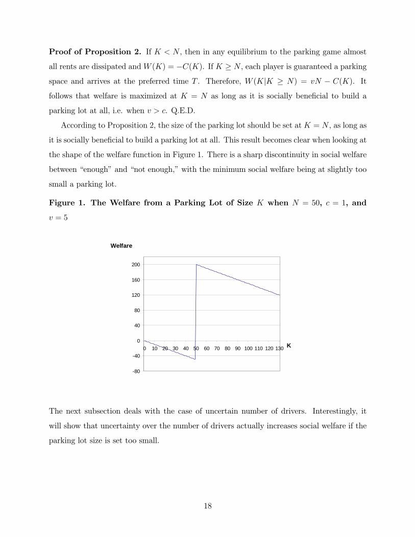
According to Proposition 2, the size of the parking lot should be set atK = N , as long as
it is socially beneficial to build a parking lot at all. This result becomes clear when looking at
the shape of the welfare function in Figure 1. There is a sharp discontinuity in social welfare
between “enough” and “not enough,” with the minimum social welfare being at slightly too
small a parking lot.
Figure 1. The Welfare from a Parking Lot of Size K when N = 50, c = 1, and
v = 5
-80
-40
0
40
80
120
160
200
0 10 20 30 40 50 60 70 80 90 100 110 120 130 K
Welfare
The next subsection deals with the case of uncertain number of drivers. Interestingly, it
will show that uncertainty over the number of drivers actually increases social welfare if the
parking lot size is set too small.
18

5.2. Optimal Capacity under Uncertainty
Assume that all drivers know the demand for parking before they choose their arrival times,
but the planner has to decide on the size of the parking lot before uncertainty about demand
(the value of N) is resolved. Maximization of expected welfare then requires a much bigger
parking lot than the expected value of potential demand, because the loss function in Figure 1
is asymmetric. In a stochastic model, there will be usually many empty spaces in a lot of
optimal size. Planners should not be tempted to increase the number of parking permits,
although unsophisticated observers may decry the wastefulness of building parking lots that
are too large or of cruelly limiting the number of permits despite the presence of unused
parking spaces.
Suppose the number of players who seek parking is uncertain and is drawn from a known
probability distribution, f(N). What is the optimal size of the parking lot? When there
is competition for parking spots, K < N , the benefit from the parking lot is negative,
W = −cK. When the size of the lot is large enough, K ≥ N , the benefit to N players is
W = vN − cK. Expected welfare is
EW (K) = vKXN=0
Nf(N)− cK = vE(N |N ≤ K)− cK (8)
The size of the parking lot should be increased as long as the marginal net benefit is non-
negative
EW (K)−EW (K − 1) = vKf(K)− c ≥ 0 (9)
Since drivers benefit from the Kth parking space only if N = K, the welfare increase
equals the probability that there are exactly K drivers multiplied by the extra benefit from
eliminating rent-seeking behavior, vK, net of the cost. The intuition is that it is more
important to have a big parking lot as K gets bigger, because there are more people who
could get benefit from it. At the same time, it could be less likely that larger parking lots
are filled out. Whether the marginal benefit of a parking space is decreasing or increasing
depends on the relative strengths of the two effects.
19

Inequality (9) can be rewritten as
Kf(K) ≥ c/v (10)
Expansion of the parking lot is welfare-improving if the probability that exactly K drivers
compete for K parking spaces times the size of the parking lot exceeds the relative cost
of building a parking space, c/v. Next we apply the theory to the uniform and binomial
distributions of N , and present the analysis of the parking problem when the number of
drivers is large and calculus methods can be employed.
Example 1: The Uniform Distribution
Consider a discrete uniform distribution on the support {0, ..., N} with p.d.f. f(N) =
1/(N + 1). Notice that for larger capacity levels, the benefit from building an additional
space in equation (9) is higher. It is equally likely at any capacity that the parking demand
will be just met, and at a larger capacity benefits accrue to more people. Hence, there is
no interior solution. With a uniform distribution, the parking lot should be big enough
to include all the people who might possibly want to park, if it should be built at all. A
comparison between EW (0) = 0 and EW (N) = (v/2− c)N reveals that the parking lot of
size large enough to accommodate all potential demanders should be constructed as long as
v/2− c > 0. On average, 50% of the parking spaces will be unclaimed since E(N) = N/2.
A parking lot is desirable if the expected value of a spot, v/2, exceeds its cost, c.7
Under uncertainty, the expected welfare isEW (K|K < N) = (v/2)(K+1)K/(N+1)−cK
and EW (K|K ≥ N) = vN/2 − cK. We can compare the expected welfare at different
capacity levels under uncertainty to the welfare under certainty (with the expected number
of drivers, N/2, arriving for sure). When N/2 drivers are arriving to the parking lot with
certainty, the welfare is W (K|K < N/2) = −cK and W (K|K ≥ N/2) = vN/2 − cK.
Table 1 and Figure 2 show the expected welfare for the uncertainty case and welfare for the
certainty case at different capacity levels when c = 1, v = 5, and N = 100.
7For any probability distribution, f(·), such that the optimal capacity size is equal to the upper bound ofthe support of the distribution, capacity utilization is equal to the ratio of the expected number of driversto the maximum number of drivers, E(X) = E(N)/N . The parking lot should be build only if the expectedvalue is no less than the cost, vE(N) ≥ cN .
20

Table 1. Welfare and Parking Lot Size when the Number of Drivers Is Uniformly
Distributed
Number of Spaces, K 0 10 20 30 40 50 60 70 80 90 100
Expected Welfare (Uncertainty) 0 -7 -10 -7 1 13 31 53 80 113 150
Welfare (Certainty, N = 50) 0 -10 -20 -30 -40 200 190 180 170 160 150
Notes: Welfare is rounded to the nearest integer.
Figure 2. Welfare and Parking Lot Size when the Number of Drivers Is Uniformly
Distributed
-80
-40
0
40
80
120
160
200
0 10 20 30 40 50 60 70 80 90 100 110 120 130 K
Welfare
EWW
Compare the consequences of a limited capacity for certain and uncertainN . Uncertainty
over the number of drivers actually increases social welfare if the parking lot size is set too
small. While the optimal capacity under uncertainty is K∗ = 100, even if K = 40, welfare is
positive. This is a big difference from the case without uncertainty, where it would be near
its minimum and very negative. The reason is that under uncertainty, even with very few
parking spaces, it may happen that very few people need to park, and so there is no wasteful
rent-seeking and the parking spaces are valuable.
21

This is somewhat paradoxical. In the first-best solution, when people are allocated to
parking spots, welfare would be highest under certainty since no parking spot would ever go
unused and no driver would ever fail to find a parking spot. The same is true when drivers
are not strategically changing their arrival schedules in attempt to secure a spot. Uncertainty
would make some excess capacity optimal, but would reduce welfare. If people are strategic,
however, the consequences of mistaken policy lead to quite different outcomes. Having a
slightly too small a parking lot would be disastrous under certainty, with zero flow payoff,
but under uncertainty the flow payoffs would be positive. Importantly, empty parking spaces
are not an indication that the parking lot is big enough. That will happen sometimes even
in a very inefficient equilibrium.
Example 2: The Binomial Distribution
Consider a binomial distribution, which arises when drivers’ needs for parking are inde-
pendent random trials and suppose that each of 100 drivers will need parking with probability
θ. A numerical example for c = 1, v = 5, N = 100, and θ = 0.5 is used as an illustration. For
these parameter values, Table 2 and Figure 3 show the expected welfare for the uncertainty
case and welfare for the certainty case at different capacity levels.
Table 2. Welfare and Parking Lot Size when the Number of Drivers Is Binomially
Distributed
Number of Spaces, K 0 10 20 30 40 50 60 70 80 90 100
Expected Welfare (Uncertainty) 0 39 78 117 153 182 189 180 170 160 150
Welfare (Certainty, N = 50) 0 -10 -20 -30 -40 200 190 180 170 160 150
Notes: Welfare is rounded to the nearest integer.
22

Figure 3. Welfare and Parking Lot Size when the Number of Drivers Is Binomi-
ally Distributed
-100
-50
0
50
100
150
200
250
0 10 20 30 40 50 60 70 80 90K
Welfare
EWW
In this example, the size of the parking lot should be K∗ = 58. Only about 8 out of 58
spaces are empty, on average. This corresponds to 86% utilization level.
Example 3: A Large Number of Drivers: The Calculus Approach
For large N we can abstract from the integer problem and use calculus. The expected
welfare from the parking lot of size K is then
EW (K) = v
Z K
0
Nf(N)dN − cK (11)
The optimal size of the parking lot is the solution to the first-order condition ∂EW (K)/∂K =
vKf(K)− c = 0, which can be re-written as
Kf(K) = c/v (12)
We can use (12) to find the optimal level of K if the maximand in (11) is concave.
Surprisingly, that seems unlikely. The second-order condition, ∂2EW (K)/∂K2 < 0, requires
Kf 0(K) + f(K) < 0. This means that the probability distribution function has to be
23
declining faster than 1/K in the relevant range of K. This is true for some distribution
functions, however, as we will see next.
Example. Consider a continuous p.d.f. f(N) = N−β with β ∈ (1, 2), defined on the support
[a, b] = [1, (2− β)1
1−β ]. Note thatR baN−βdN = 1 and the mean number of drivers in need of
parking is E(N) =R baNf(N)dN =
¡b2−β − 1
¢/(2− β).
The first-order condition implies the optimal capacity K∗ = (c/v)1/(1−β), and the second-
order condition is satisfied. The mean utilization of the parking lot of optimal size can
be measured as a ratio of the mean number of parking spots taken, E(X), to the opti-
mal capacity size, K∗. If N < K, then all N drivers find parking; if N ≥ K, then K
out of N drivers find parking. Hence, E(X) =R K∗aNf(N)dN +
R bK∗K
∗f(N)dN . The
mean capacity utilization as a percentage of the optimal lot size is, therefore, E(X)/K∗ =³(c/v)− (c/v)
1β−1 (β − 1)− (2− β)2
´/ ((2− β) (β − 1)). For example, when c/v = 0.5 and
β = 1.5, K∗ = 4 and E(X) = 2. (Keep in mind that the number of drivers must be large
for the analysis of this section to be correct, so “4” might denote 4 thousand drivers.) On
average, 50% of the parking spots will remain unoccupied. The 50%-utilized parking lot is
socially optimal.
The expected welfare for a parking lot of size K, relative to the value v of parking, is
EW (K)/v =R K1N1−βdN−(c/v)K =
¡K2−β − 1
¢/(2−β)−(c/v)K. To compare the results
to those under no uncertainty, suppose that the distribution for N is degenerate, taking value
N = E(N) for sure. Under no uncertainty, the optimal lot size is E(N). The welfare from
the parking lot is W (K = E(N)) = (v − c)E(N).
Table 3 compares welfare at different capacity levels for a variety of parameter combina-
tions.
24

Table 3. Capacity Utilization and Expected Welfare
Parameter Values
Welfare Measures c/v = 0.4 c/v = 0.5 c/v = 0.6β = 1.6 1.7 1.8 β = 1.6 1.7 1.8 β = 1.6 1.7 1.8
E(N) 2.11 2.25 2.48 2.11 2.25 2.48 2.11 2.25 2.48K∗ 4.61 3.70 3.14 3.17 2.69 2.38 2.34 2.07 1.89
Capacity Utilization (%) 45.71 57.59 65.95 62.92 71.41 77.28 76.63 82.18 85.97
aWelfare, W (E(N))/v 1.26 1.35 1.49 1.05 1.13 1.24 0.84 0.90 0.99
bWelfare, EW (K∗)/v 2.11 1.60 1.29 1.47 1.15 0.95 1.01 0.82 0.68
cWelfare EW (K00)/v 0.26 0.12 0.03 - 0.12 -0.19 -0.24 -0.39 -0.43 -0.46
Notes: K∗ is the optimal size of the parking lot under uncertainty. a) No uncertainty,
K = E(N); b) Uncertainty, K = K∗; c) Uncertainty, K 00 = 0.99K∗ - capacity is 1% below
optimal.
Table 3 illustrates our assertion that a slightly too small parking lot can be worse than no
parking lot at all. In case (c), the size of the parking lot is one percent below the optimal
level, and this small change greatly affects the expected welfare.
6. Discussion of Inter-Driver Contracting, the Assumption of Dis-crete Time, and the Parking Lot Cost Function
The rent-seeking behavior of drivers can be avoided by either increasing the capacity level
or by restricting the entry to the facility. Under certainty, if there are K parking spaces
and N > K people willing to park, access should be restricted to K people. If more people
were given parking permits, the competition would not allow them to obtain benefit from
parking. The effect of extra parking permits would be to reduce the benefit for the original
permit holders to zero.
If binding contracts could be made, the problem would be avoided. Everyone would arrive
at T , K people would take the parking spaces, and the other N−K would get side payments
25

from the ones who park in the desirable lot. This, however, requires (a) communication to
coordinate who parks, (b) low enough transaction costs for coordinating and making the
payments, and (c) enforceability at low cost, so that people do not break their contract and
arrive early or refuse to make the side payments later.8
We have modeled the parking game in discrete rather than continuous time for a number
of reasons. A discrete-time framework is better describing situations when players can choose
time of arrival from a given set of permissible times. For example, when the model is
interpreted as describing the timing of purchases by bargain hunters, the decision may be
to arrive on Friday, Saturday, or Sunday during the sales period. When time is continuous,
there are no “alternating” equilibria of the kind described in Claims 1 and 2 since there does
not exist “the next time.” An attractive property of discrete-time equilibria is that they
permit two or more players to arrive at the same time. The probability of such a tie is zero
for atomless strategies in continuous time. Moreover, continuous time may be considered a
limiting case of the discrete time as the time grid becomes infinitely fine.
One way to specify strategies in continuous time under unobservability would be to
consider cumulative distribution functions for players’ arrival times. This approach results
in complete rent dissipation in any equilibrium, as Barut and Kovenock (1998) demonstrate.
It follows from Theorem 2 in Barut and Kovenock (1998) that the expected payoff of any
player is zero in any (mixed-strategy) equilibrium under unobservability when N > K ≥ 1.
Hence, under unobservability the full rent dissipation result extends to the continuous-time
framework. Under full observability, players’ strategies have to be conditioned on the history
of arrivals to the parking lot, which cannot be captured with the traditional approach of
finding equilibrium cumulative distribution functions for players’ arrival times, and presents
technical difficulties.
It is easy to extend the analysis of the optimal capacity choice to allow for an arbitrary
cost function, C(K). Due to the full rent dissipation result, the planner would still choose
8In 1999 a Ticket Master in Windsor, Ontario, used an interesting approach to distributing tickets. Toprevent the practice of overnight lineups and discourage scalping a random number line-up procedure wasadopted. This approach assigns a random number to each ticket buyer present at the time the office isopening and the queue is formed accordingly. While the procedure may appear unfair to many ticket buyers,it eliminates incentives to arrive early camping over night or long hours of waiting in line by providing eachcustomer with a fair and equitable opportunity to be first in line. The case is reported, among with manyother queueing examples, at http://www2.uwindsor.ca/˜hlynka/qreal.html.
26

to guarantee each driver a parking space when N is certain, or not build the parking lot
at all.9 In contrast, we conjecture that when drivers value parking spots asymmetrically,
guaranteeing every driver a spot may not be optimal. The social planner has to choose the
capacity, K, to maximize the welfare, measured by the cumulative value of the parking lot
to drivers net of the cost of capacity. The planner faces a trade-off between the production
cost and the cost of wasteful rent-seeking. When capacity is at least as high as the number
of players, players are guaranteed parking spaces and there is no competition for the spaces.
Since extra spaces are costly, no excess capacity is build in the case of the certain number
of players. The planner chooses between guaranteeing a parking space for each driver and
staging a contest, and even under certainty, a contest may be preferred if the cost is convex.10
7. Concluding Remarks
We have constructed various versions of a parking lot model, focusing not so much on
planning for uncertain demand as on planning for strategic behavior by the demanders.
Suppose 1,001 drivers want to arrive at the same time and have the same costs of arriving
early, and each derives a benefit of $250 from parking there during the year. Then if the
cost of a parking space is $200 per year, it is obvious that 1,001 spaces should be built, for
a net payoff of $50,050 per year. What is not so obvious, and what has been the theme of
this paper in various models, is that if 1,000 spaces are built instead, the net payoff is not
$50,000, but rather -$200,000. Competition in the form of early arrival for the scarce spots
eats up the entire benefit from the parking lot. Of course, the implications of a shortage may
9When parking spaces are of different values, for example, due to variations in proximity and/or con-venience, the rent dissipation result may still hold. For all-pay auctions cast in continuous space underunobservability, Barut and Kovenock (1998) establish full rent dissipation for arbitrary prize valuations,provided all players are not guaranteed the same prize value.10Clark and Riis (1998) establish a rent dissipation result for a multi-prize all-pay contest with asymmetric
valuations for the unobservability case and continuous strategy space. Their Proposition 1 implies that theexpected net surplus from K identical parking spaces, valued as vi by player i, is
PKi=1 (vi − vK+1) when
K < N . Hence, in this framework the expected welfare is W (K|K < N) =PKi=1 (vi − vK+1) − C(K).
The planner would increase the size of the parking lot from (K − 1) to K if the marginal benefit is no lessthan the marginal cost, i.e., if C(K) − C(K − 1) ≤ (v(K)− v(K + 1))K. Staging the contest between
drivers for parking spaces is preferred when W (K|K < N) > W (K = N), which can be written as C(N)−C(K) ≥
PNi=K∗+2 vi+
PK∗+1i=1 vK∗+1. The first summation term corresponds to an increase in the number of
beneficiaries from K∗ to N and the second summation term is due to the lack of rent-seeking when parkingis guaranteed.
27

not be as dramatic when, for example, the number of drivers is uncertain, but this extreme
case shows the nature of the problem.
Thus, strategic incentives are an essential element in planning capacity for an underpriced
good — as important, or perhaps more important, than the obvious decision-theory problem
of predicting uncertain demand and the obvious engineering problem of predicting capacity
cost. If for some reason direct pricing is impractical, and the planner is aware that some of
the time demand for the good could exceed the supply, he should realize that the damage
from such situations in not limited to just a few people finding the good has run out,
because people’s actions to forestall being thus shut out can vastly increase the damage.
Civil engineers need to understand game theory.
28

Appendix: Proof of Claim 4
Claim 4. In any equilibrium with more drivers than parking spaces, the probability that the
parking lot is full at time t ≤ T is one under full observability and approaches one as the
time grid becomes infinitely fine under unobservability. The equilibrium payoffs of players
who arrive at t with a positive probability are zero under full observability and they tend to
zero under unobservability as the time grid becomes infinitely fine. Any player who arrives
at t tends to dissipate all the rent from parking.
Proof. Consider a subgame-perfect equilibrium to the parking game under full observability
or unobservability. By the definition of t, there is a player who does not arrive with a pure
strategy before t. The player (player i) who some times arrives at t should be unwilling to
deviate by arriving at t −∆ with a pure strategy, while keeping his arrival schedule before
t −∆ the same. Note that t is either equal to the time when the parking lot becomes full
for sure, denoted by t0, or the preferred time, T, since no players arrive between t0 and T .
Player i’s payoff from arriving at t, for given Kt−∆ and the number of other players who
happen to arrive at t−∆, n, is
ui,t|Kt−∆,n = pi,t · v (A1)
where
pi,t =Kt
Nt< 1 (A2)
is the probability that player i obtains parking at t, Kt = max{Kt−∆ − n, 0} and Nt =
N −K +Kt.
For given Kt−∆ and n, player i’s payoff from arriving at t−∆ is
ui,t−∆|Kt−∆,n = pi,t−∆ · v − w∆ (A3)
where
pi,t−∆ = min
½Kt−∆n+ 1
, 1
¾(A4)
29

is the probability that player i obtains parking at t−∆ conditional on Kt−∆ parking spaces
available at t−∆ and n other players arriving at t−∆.
Three possibilities arise for different values of Kt−∆ and n.
Case 1: If Kt−∆ = 0, then pi,t = 0 and pi,t−∆ = 0.
Case 2: If 0 ≤ n < Kt−∆, then pi,t = Kt/(N −K +Kt) < 1 and pi,t−∆ = 1.
Case 3: If n ≥ Kt−∆ > 0, then pi,t = 0 and pi,t−∆ = Kt−∆/(n+ 1) > 0.
Cases 1-3 show that unless Kt−∆ = 0, arriving at t−∆ provides player i with a strictly
higher odds of obtaining parking. If 0 ≤ n < Kt−∆, then pi,t−∆ − pi,t = (N −K)/(N −K +
Kt−∆−n) > 0. If n ≥ Kt−∆ > 0, then pi,t−∆−pi,t = Kt−∆/(n+1) > 0. Finally, if Kt−∆ = 0,
then pi,t−∆ − pi,t = 0.
Under full observability, player i’s deviation is not profitable for a givenKt−∆ if inequality
ui,t|Kt−∆ − ui,t−∆|Kt−∆ ≥ 0 holds. The inequality can be written as
Nt−∆−1Xn=0
Pr(n) ·¡pi,t−∆ − pi,t
¢· v ≤ w∆. (A5)
Inequality (A5) always holds if Kt−∆ = 0 since player i does not increase his odds of
obtaining parking when the parking lot is already full at t −∆. When Kt−∆ = 0, player i
chooses to arrive at T . If there exists a parking space at t−∆ (i.e.,Kt−∆ > 0), a player who is
supposed to arrive at t will always deviate by arriving with a pure strategy at t−∆, keeping
the arrival schedule before t−∆ unchanged. This is because the deviation increases player i’s
odds of obtaining parking by a positive amount bounded away from zero and the additional
cost of the earlier arrival approaches zero. In other words, since the right-hand side of (A5)
goes to zero as time grid becomes infinitely fine, the left-hand side of the inequality has to
be converging to zero as well. This is not possible for Kt−∆ > 0 since pi,t−∆ − pi,t 9 0
and Pr(n) 9 0 for some n. To summarize, if Kt−∆ = 0, player i arrives at t − ∆ while if
Kt−∆ > 0, player i arrives at T . This is consistent with our assumption that player i arrives
at t with a pure strategy (conditional on not arriving before t) only if t = T . Consider the
case where t = T . At least two players arrive at T with a pure strategy, conditional on not
arriving before T . If KT−∆ = 0 then KT = 0 as well, and players arriving at T receive a
zero payoff. If KT−∆ > 0, then all players who have not arrived choose to arrive at T −∆
30

since the odds of obtaining a parking spot at T −∆ are higher than at T in this case. Once
again, we obtain KT = 0. Hence, under full observability Kt = 0.
Under unobservability, player i’s deviation is not profitable if inequality ui,t − ui,t−∆ ≥ 0
holds, which can be written as
KXKt−∆=0
Nt−∆−1Xn=0
Pi,t−∆(Kt−∆) Pr(n) ·¡pi,t−∆ − pi,t
¢· v ≤ w∆ (A6)
where Pi,t−∆(Kt−∆) denotes player i’s assessment of the probability that there are Kt−∆
empty spaces at t−∆, given player i has not arrived before t−∆. Since the right-hand side
of the inequality goes to zero as time grid becomes infinitely fine, the left-hand side of the
inequality has to be converging to zero as well.
Suppose that in an equilibriumKt−∆ > 0 arises with a positive probability bounded away
from zero (i.e., there exists Kt−∆ > 0 such that Pi,t−∆(Kt−∆) 9 0). Since pi,t−∆ − pi,t > 0
for Kt−∆ > 0, we find that Pr(n) → 0 for all possible realizations of n in the equilibrium
for given Kt−∆. This is not possible sincePNt−∆−1
n=0 Pr(n) = 1. Hence Pi,t−∆(Kt−∆)→ 0 for
all Kt−∆ > 0. Under unobservability we find that almost for sure no parking is available to
player i arriving at t.
Suppose a player arriving at t with a positive probability were to obtain a positive payoff
bounded away from zero. This implies that t > t∗ +∆. For t > t∗ +∆, the player with a
nearly zero payoff at t can increase his payoff by arriving at t−∆. Hence, the payoff of the
player arriving at t approaches zero.11 Q.E.D.
11It is easy to show that the earliest and the latest time anyone arrives with a positive probability in anequilibrium approach t∗ and T respectively as the time grid becomes infinitely fine. First, we show thatt→ t∗ as ∆→ 0. If t ≤ t∗+∆, then t→ t∗. Suppose that t > t∗+∆. At t, all parking spaces are available,and the probability of obtaining a space at t converges to one because otherwise a player assigned to arriveat t would arrive at t −∆. Since the payoff at t approaches zero, t → t∗ in this case as well. Second, weshow that t→ T as ∆→ 0. Since it is nearly impossible to obtain parking at t in an equilibrium and playersreceive non-negative payoffs, the cost of arriving at t must be zero in the limit as well. Hence, t → T as∆→ 0.
31

References
[1] Anderson, Simon and Andre de Palma (2004) “The Economics of Pricing Parking,”
Journal of Urban Economics, 55, 1—20.
[2] Arnott, Richard and John Rowse (1999) “Modeling Parking,”Journal of Urban Eco-
nomics, 45, 97—124.
[3] Arnott, Richard, Andre de Palma, and Robin Lindsey (1993) “A Structural Model of
Peak-Period Congestion: A Traffic Bottleneck with Elastic Demand,” The American
Economic Review, 83, 161—179.
[4] Avery, Christopher, Christine Jolls, Richard A. Posner, Alvin E. Roth (2001) “The
Market for Federal Judicial Law Clerks,” University of Chicago Law Review, 68, 793—
902.
[5] Barut, Y. and Daniel Kovenock (1998) “The Symmetric Multiple Prize All-Pay Auction
with Complete Information,” European Journal of Political Economy, 14, 627—644.
[6] Baye, Michael R., Daniel Kovenock, and Casper G. de Vries (1996) “The All-Pay Auc-
tion with Complete Information,” Economic Theory, 8: 291—305.
[7] Clark, Derek and Christian Riis (1998) “Competition over More Than One Prize,” The
American Economic Review, 88, 276—289.
[8] Deacon, Robert T. and Jon Sonstelie (1991) “Price Controls and Rent Dissipation with
Endogenous Transaction Costs,” The American Economic Review, 81, 1361—1373.
[9] Deacon, Robert T. and Jon Sonstelie (1985) “Rationing by Waiting and the Value of
Time: Results from a Natural Experiment,” The Journal of Political Economy, 93,
627—647.
[10] Deacon, Robert T. and Jon Sonstelie (1989) “The Welfare Costs of Rationing by Wait-
ing,” Economic Inquiry, 27, 179—196.
[11] Deacon, Robert T. (1994) “Incomplete Ownership, Rent Dissipation, and the Return
to Related Investments,” Economic Inquiry, 32, 655— 683.
32

[12] Fudenberg, Drew and Jean Tirole (1985) “Preemption and Rent Equalization in the
Adoption of New Technology,” The Review of Economic Studies, 52, 383—401.
[13] Cullis, John G. and Philip R. Jones (1986) “Rationing by Waiting Lists: An Implica-
tion,” The American Economic Review 76, 250—256.
[14] Hassin, Refael (1985) “On the Optimality of First Come Last Served Queues,” Econo-
metrica, 53, 201—202.
[15] Holt, Charles A. Jr. and Roger Sherman (1982) “Waiting-Line Auctions,” The Journal
of Political Economy, 90, 280—294.
[16] Landsburg, Steven E. (1995) The Armchair Economist: Economics and Everyday Life,
Free Press (1995).
[17] Lindsay, Cotton M. and Bernard Feigenbaum (1984) “Rationing by Waiting Lists,” The
American Economic Review, 74, 404—417.
[18] Nalebuff, Barry (1989) “Puzzles: The Arbitrage Mirage, Wait Watchers, and More,”
The Journal of Economic Perspectives 3, 165—174.
[19] Naor, P. (1969) “The Regulation of Queue Size by Levying Tolls,” Econometrica, 37,
15—23.
[20] Porter, Richard C. (1977) “On the Optimal Size of Underpriced Facilities,” The Amer-
ican Economic Review, 67, 753—760.
[21] Roth, Alvin E. and Xiaolin Xing (1994) “Jumping the Gun: Imperfections and Institu-
tions Related to the Timing of Market Transactions,” American Economic Review, 84,
992—1044.
[22] Simon, Leo K. and Maxwell B. Stinchcombe (1989) “Extensive Form Games in Contin-
uous Time: Pure Strategies,” Econometrica, 57, 1171— 1214.
[23] Vickrey, William S. (1969) “Congestion Theory and Transport Investment,” The Amer-
ican Economic Review (Papers and Proceedings), 59, 251—260.
33
Recommended