Raster Data Models 2/9/2016
GEO327G/386G, UT Austin 1
2/9/2016 GEO327G/386G, UT Austin 1
The Raster Data Model
Llano River, Mason Co., TX
5 5 5 5 5 5 55
5555 5 5 2 2
2 2 8 888225555
5555
2 2 22 2 8 822 55 555522 2 22 5 5 5 5
5555225 2
2/9/2016 GEO327G/386G, UT Austin 2
Rasters are:
Regular square tessellations
Matrices of values distributed among equal-sized, square cells
565 573 582 590
575 580 595 600
579 581 597 601
580 600 620 632
2/9/2016 GEO327G/386G, UT Austin 3
Why squares?
Computer scanners and output devices use square pixels
Bit-mapping technology/theory can be adapted from computer sciences
1-to-1 mapping to grid coordinate systems!
2/9/2016 GEO327G/386G, UT Austin 4
Cell location specified by:
• Row/column (R/C) address
• Origin is upper left cell (1,1)
• Relative or geographic coordinates can be specified
1 2 3 4
1 1,1
2
3 4,3
4
6005300
6005180
510400
510520
UTM coordinates

Raster Data Models 2/9/2016
GEO327G/386G, UT Austin 2
2/9/2016 GEO327G/386G, UT Austin 5
Registration to “world” coordinates
6005300
510400
00
Unregistered Registered
2/9/2016 GEO327G/386G, UT Austin 6
Registration to “world” coordinates
6005300510400
Requires “world file”:
• Specify coords. of upper left corner
• Specify ground dimensions of cell, in same units
30 m
Image Space
X columns
Y ro
ws
Map Spacex
y
World File – DRG example
2.43840000000000 CELL SIZE IN X DIRECTION (m)
0.00000000000000 ROTATION TERM
0.00000000000000 ROTATION TERM
-2.43840000000000 CELL SIZE IN Y DIRECTION (m)
487988.64154709835000 UTM EASTING OF UPPER LEFT CORNER (m)
3401923.72301301550000 UTM NORTHING OF UPPER LEFT CORNER (m)
/* UTM Zone 14 N with NAD83
/* This world file shifts the upper left image coordinate to the corresponding
/* NAD83 location, resulting in an approximated NAD83 image.
/* Map Name: Art
/* Map Date: 1982
/* Map Scale: 24000
2/9/2016 GEO327G/386G, UT Austin 7 2/9/2016 GEO327G/386G, UT Austin 8
Spatial Resolution
Defined by area or dimension of each cell
o Spatial Resolution = (cell height) X (cell width)
o High resolution: cell represent small area
o Low resolution: cell represent larger area
Defined by size of one edge of cell (e.g. “30 m DEM”)
For fixed area, file size increases with resolution
40 m40 mHi Res.Low Res.
100 m2 25 m2
10 m 5 m

Raster Data Models 2/9/2016
GEO327G/386G, UT Austin 3
2/9/2016 GEO327G/386G, UT Austin 9
30 m vs. ~90 m pixel size
Packsaddle Mountain
(50 m contours, vector data layer)
o Resolution of 30 m data is 9 times better than 90 m data
30 m 90 m
2/9/2016 GEO327G/386G, UT Austin 10
Resolution constraint
Cell size should be less than half of the size of the smallest object to be represented (“Minimum mapping unit; MMU”)
Cell size = MMU Cell size ~ ½ MMU
2/9/2016 GEO327G/386G, UT Austin 11
e.g. DOQQ resolutions
Resolution is size of sampled area on ground, not MMU
1 m2 1/3 m
MMU= 2 m MMU= ~ 2/3 m
(E. Mall Circle Drive)
“1 m” “1/3 m”
“1 m resolution ”
raster data
“1/3 m resolution ”
raster data
565 573 582 590
575 580 595 600
579 581 597 601
580 600 620 632
2/9/2016 GEO327G/386G, UT Austin 12
Raster Dimension:
Number of rows x columns
o E.g. Monitor with 1900 x1200 pixels
Dimension = 4 x 4

Raster Data Models 2/9/2016
GEO327G/386G, UT Austin 4
2/9/2016 GEO327G/386G, UT Austin 13
Raster Attributes
Two types:
1. Integer codes assigned to raster cells
E.g. rock type, land use, vegetation
Codes are technically nominal or ordinal data
2. Measured “real” values
Can be integer or “floating-point” (decimal) values; technically interval or ratio data
E.g. topography, em spectrum, temperature, rainfall, concentration of a chemical element
2/9/2016 GEO327G/386G, UT Austin 14
Integer Code Attributes
Code is referenced to attribute via a “look-up table” or “value attribute table” – VAT
Commonly many cells with the same code
Different attributes must be stored in different raster layers
5 5 5 5 5 5 55
5555 5 5 2 2
2 2 8 888225555
5555
2 2 22 2 8 822 55 555522 2 22 5 5 5 5
5555225 2
Value Count Rock Type
2 21 Marble
5 37 Gneiss
8 6 Granite
VAT
Nominal Coded Raster
2/9/2016 GEO327G/386G, UT Austin 15
Mixed Pixel Problem
Severity is resolution dependant
Rules to assign mixed pixels include:
• “edge pixels”: not assigned to any feature– define a new class
• Assign to feature that comprises most of pixel
2/9/2016 GEO327G/386G, UT Austin 16
Coded Value Raster Types
Single-band: Thematic datao Black & White: binary (1 bit) (0 = black, 1 = white)
o Panchromatic (“Grayscale”) (8 bit): 0 (black) – 255 (white) or graduated color ramps (e.g. blue to red, light to dark red)
o Colormaps (“Indexed Color”) (8 bit): code cells by values that match prescribed R-G-B combinations in a lookup table
Figures from: Modeling our World, ESRI press
Lookup/index tableB & W Panchromatic Color Map

Raster Data Models 2/9/2016
GEO327G/386G, UT Austin 5
2/9/2016 GEO327G/386G, UT Austin 17
Single Band
Examples – Black & White (Grayscale)
Grayscale – 8 bit;
Black & White - 1 bit54
black, white & 254 shades of gray
2/9/2016 GEO327G/386G, UT Austin 18
Single BandExample Color Map (Indexed Color)
Each pixel contains one of 12 unique values, each corresponding to a prescribed color (Red, Green & Blue combination)
(10 of 12 values shown)
E.g. Austin East 7.5’ Digital Raster Graph
2/9/2016 GEO327G/386G, UT Austin 19
Measured, “Real Value” Attributes
Commonly stored as floating point values
Different attributes must be stored in different layers, e.g. spectral bands in satellite imagery
Compression techniques for rasters of integer-valued cells, but not floating point (see below)
2/9/2016 GEO327G/386G, UT Austin 20
MultibandImage Raster Attributes
Multi-band Spectral Data Band 3
Band 2
Band 1
Visible Spectrum
Band = segment of Em spectrum
Map intensities of each band as red, green or blue.
Display alone or as composite
RGB Composite
Red
Green
Blue
Attribute values0 - 255
255
0
Figures from: Modeling our World, ESRI press

Raster Data Models 2/9/2016
GEO327G/386G, UT Austin 6
2/9/2016 GEO327G/386G, UT Austin 21
Multiband Image 8 bits/Band, 3 Band RGB
Band 1
Band 2
Band 3
E.g. Austin East 7.5’ Color Infrared Digital Orthophotograph (“CIR DOQ”)
2/9/2016 GEO327G/386G, UT Austin 22
Cell values apply to:
Middle of cell, e.g. Digital Elevation Models (DEM)
Whole cell, e.g. most other data
Source: Modeling our World, ESRI press
2/9/2016 GEO327G/386G, UT Austin 23
Digital Elevation Model
Southern Tetons, Wyoming
2/9/2016 GEO327G/386G, UT Austin 24
Airborn Magnetic (TFI) Map
Southern Tetons, Wyoming
TFI Pixel values
Raster Data Models 2/9/2016
GEO327G/386G, UT Austin 7
2/9/2016 GEO327G/386G, UT Austin 25
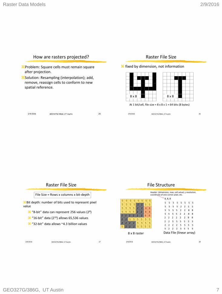
How are rasters projected?
Problem: Square cells must remain square after projection.
Solution: Resampling (interpolation); add, remove, reassign cells to conform to new spatial reference.
2/9/2016 GEO327G/386G, UT Austin 26
Raster File Size
fixed by dimension, not information
At 1 bit/cell, file size = 8 x 8 x 1 = 64 bits (8 bytes)
8 x 88 x 8
2/9/2016 GEO327G/386G, UT Austin 27
Raster File Size
File Size = Rows x columns x bit-depth
Bit depth: number of bits used to represent pixel value
“8-bit” data can represent 256 values (28)
“16-bit” data (216) allows 65,536 values
“32-bit” data allows ~4.3 billion values
2/9/2016 GEO327G/386G, UT Austin 28
File Structure
5 5 5 5 5 5 5
5
5
555 5 5 2 2
2 2 8 8
88225555
5555
2 2 22 2 8 82
2 55 55552
2 2 22 5 5 5 5
5555225 2
8 x 8 raster
5 5 5 5 5 5 5
5
5
555 5 5 2 2
2 2 8 8
88225555
5555
2 2 22 2 8 82
2 55 55552
2 2 22 5 5 5 5
5555225 2
8, 8, 8
Data File (linear array)
Header: (dimension, max. cell value) + resolution, coordinate of one corner pixel, etc.
Raster Data Models 2/9/2016
GEO327G/386G, UT Austin 8
2/9/2016 GEO327G/386G, UT Austin 29
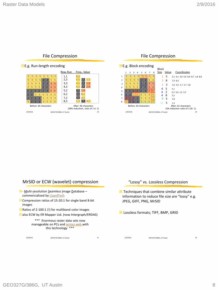
File Compression
E.g. Run-length encoding
1,1 8,5
Row, Run Freq., Value
2,3 4,5 2,2 2,53,3 4,5 2,2 2,84,3 4,5 2,2 2,85,2 6,2 2,86,2 2,2 6,5
7,2 4,2 4,58,3 1,5 3,2 4,5
5 5 5 5 5 5 5
5
5
555 5 5 2 2
2 2 8 8
88225555
5555
2 2 22 2 8 82
2 55 55552
2 2 22 5 5 5 5
5555225 2
Before: 64 characters After: 46 characters (28% reduction; ratio of 1.4: 1)
2/9/2016 GEO327G/386G, UT Austin 30
File Compression
E.g. Block encoding
1 5 5,1 6,1 3,6 4,6 8,6 8,7
Block Size Value Coordinates
1,8 8,8
4 5 7,1
1 2 3,5 4,5 1,7 2,7 2,8
9 5 5,6
16 5 1,1
5 5 5 5 5 5 5
5
5
555 5 5 2 2
2 2 8 8
88225555
5555
2 2 22 2 8 82
2 55 55552
2 2 22 5 5 5 5
5555225 2
Before: 64 characters After: 61 characters(5% reduction ratio of 1.05: 1)
1 2 3 4 5 6 7 8
1
2
3
4
5
6
7
8
4 8 7,3
4 2 5,2 5,4 1,5 3,7
1 8 7,5 6,5
2/9/2016 GEO327G/386G, UT Austin 31
MrSID or ECW (wavelet) compression
- Multi-resolution Seamless Image Database –commercialized by LizardTech
Compression ratios of 15-20:1 for single band 8-bit images
Ratios of 2-100:1 (!) for multiband color images
also ECW by ER Mapper Ltd. (now Intergraph/ERDAS)
*** Enormous raster data sets now manageable on PCs and across web with
this technology ***
2/9/2016 GEO327G/386G, UT Austin 32
“Lossy” vs. Lossless Compression
Techniques that combine similar attribute information to reduce file size are “lossy” e.g. JPEG, GIFF, PNG, MrSID
Lossless formats; TIFF, BMP, GRID

Raster Data Models 2/9/2016
GEO327G/386G, UT Austin 9
2/9/2016 GEO327G/386G, UT Austin 33
Raster Pyramids
Store reduced-resolution copies of a raster for rapid display – e.g ArcGIS, Google, many others
Often combined with image tiling for rapid rendering of images
Source: ESRI ArcGIS Help file
2/9/2016 GEO327G/386G, UT Austin 34
Image “Tiling”
Split raster into small contiguous rectangles or squares = tiles
Display only the tile required upon zooming
2/9/2016 GEO327G/386G, UT Austin 35
Level 0 = 100% of image = 16 low res. tilesLevel 1 = higher res. (parts of 4 med. res. tiles)Level 2 = highest res. (1+ high res. tiles)
Level 0
Level 1
Level 2
2/9/2016 GEO327G/386G, UT Austin 36
Supported Raster Formats
See ArcCatalog>Tools>
Options
Each explained in Help
o 24 supported formats

Raster Data Models 2/9/2016
GEO327G/386G, UT Austin 10
2/9/2016 GEO327G/386G, UT Austin 37
Vector or Raster?
Spatially continuous data = raster
Modeling of data with high degree of variability = raster
Objects with well defined boundaries = vector
Geographic precision & accuracy = vector
Topological dependencies = vector or raster
2/9/2016 GEO327G/386G, UT Austin 39
Raster or Vector?
Raster Simple data structure
Ease of analytical operation
Format for scanned or sensed data – easy, cheap data entry
But…….
Less compact
Querry-based analysis difficult
Coarser graphics
More difficult to transform & project
Vector Compact data structure
Efficient topology
Sharper graphics
Object-orientation better for some modeling
But….
More complex data structure
Overlay operations computationally intensive
Not good for data with high degree of spatial variability
Slow data entry
Recommended