Calhoun: The NPS Institutional Archive
Theses and Dissertations Thesis Collection
1987
An evaluation of Interactive Laboratory System software
Quintero, Thomas A.
http://hdl.handle.net/10945/22784


DUDLEY KNOX LIBRARYCHOOL ^
I
-


NAVAL POSTGRADUATE SCHOOL
Monterey , California
THESIS
AN EVALUATION OF INTERACTIVE LABORATORYSYSTEM SOFTWARE, ILS
PC/DOS, A DIGITAL SIGNAL PROCESSINGSOFTWARE PACKAGE
by
Thomas A. Quintero• * $
December 1987
Thesis AdvIsor D. E. Kirk
Approved for public release; distribution is unlimited.
T239137

REPORT DOCUMENTATION PAGEla REPOR* SECURITY ClASSiF.CAT ON
UnclassifiedId RESTRICTIVE MARk.NGS
2a SECURITY MASSIF.CATiON AuThOR'T' 3 DISTRIBUTION/ AVAILABILITY OF REPORT
Approved for public release;Distribution is unlimited2D DECLASSIFICATION /DOWNGRADING SCHEDULE
4 PERFORMING ORGANIZATION REPORT NuMBER(S) 5 MONITORING ORGANIZATION REPORT NuMBER(S)
6a NAME Or PERFORMING ORGANlZAT.ON
Naval Postgraduate School
6o OFFiCE SYMBOL(If applicable)
7a NAME OF MONITORING ORGANIZATION
Naval Postgraduate School
6c ADDRESS [City, State, and ZIP Code)
Monterey, California 93943-5100
7D ADDRESS (C/fy, Stare, and ZIP Code)
Monterey, California 93943-5100
8a NAME 0= FUNDING SPONSORINGORGANIZATION
8b OFF.CE SYMBOL(If applicable)
9 PROCUREMENT INSTRUMENT IDENTIFICATION NUMBER
8c. ADDRESS (City, State, and ZIP Code) 10 SOURCE OF FUNDING NUMBERS
PROGRAMELEMENT NO
PROJECTNO
TASKNO
WORK UNITACCESSION NO
11. TITLE (include Security Classification)
AN EVALUATION OF INTERACTIVE LABORATORY SYSTEM, ILS-PC/DOS, A DIGITAL SIGNALPROCESSING SOFTWARE PACKAGE
12 =ERSONA,_ AJTHOR(S)Quintero, Thomas A.
13a TYPE OF RE DORTMaster's Thesis
3D T ME COVE°ED=ROM ~0
4 DATE OF REPORT ( Year, Month. Day)
1987 December 1615 PAGE COUNT
85
16 SUPPLEMENTARY NOTA T iON
17 COSAT CODES '8 S^BJEC^ TERMS (Continue on reverse if necessary and identify by bloc* number)
= ELD GROUP SUB GROUP Digital Signal Processing Software
19 ABSTRACT '.Continue on reverse if necessary and identify by block number)
An evaluation is presented of the Interactive Laboratory System'sdigital signal processing software. The capabilities of the softwareare outlined and several representative problems are solved. Acomparison is made of this software package with existing signalprocessing tools at the Naval Postgraduate School.
20 DiSTR'BUTiON. AVAILABILITY OF ABSTRACT
C3 unclassified;unlimi ted SAME as rpt Q dtic USERS
21 ABSTRACT SECURITY CLASSIFICATION
Unclassified22a NAME OF RESPONSIBLE INDIVIDUALKirk, Donald E.
22b TELEPHONE (Include Area Code)
(415) 646-3451.:2c OFFiCE SYMBOL600
DD FORM 1473,34 war 83 APR edition may oe used until exhausted
All other editions are obsoleteSECURITY CLASSIFICATION OF T HIS PAGE
ft US Government Printing C'lce 1986—SOS
Approved for public release; distribution is unlimited.
An Evaluation of Interactive Laboratory System Software, ILSPC/DOS, a Digital Signal Processing Software Package
bv
Thomas A. QuinteroCaptain, United States Marine Corps
B.S., United States Naval Academy, 1981
Submitted in partial fulfillment of the
requirements for the degree of
MASTER OF SCIENCE IN ELECTRICAL ENGINEERING
from the
NAVAL POSTGRADUATE SCHOOLDecember 1987
ABSTRACT
An evaluation is presented of the Interactive Laboratory System's digital signal
processing software. The capabilities of the software are outlined and several
representative problems are solved. A comparison is made of this software package
with existing signal processing tools at the Naval Postgraduate School.
11
TABLE OF CONTENTS
I. DIGITAL SIGNAL PROCESSING SOFTWARE S
A. INTRODUCTION 8
B. NEED FOR DIGITAL SIGNAL PROCESSINGSOFTWARE 8
C. DIGITAL SIGNAL PROCESSING SOFTWAREPACKAGE REQUIREMENTS S
1. Personal Computer Based Software 8
2. Signal Processing Capabilities 9
II. USING ILS 11
A. DESCRIPTION OF ILS 11
1. Operation of ILS 11
2. Capabilities of ILS 13
3. Summary 14
B. GUIDE TO PROBLEM SOLVING WITH ILS 14
1. Problem Solving Technique 14
2. Problem Solving Techniques With ILS 14
C. PROBLEM SOLVING WITH ILS 15
1. ILS Files 15
2. Using ILS Files 16
III. SOLVING PROBLEMS WITH ILS 18
A. DIGITAL FILTER DESIGN" 18
B. SPECTRAL ANALYSIS 35
IV. CONCLUSIONS 66
A. DIGITAL SIGNAL PROCESSING TOOLS AT NTS 66
B. ADVANTAGES AND DISADVANTAGES OF ILS 66
C. RECOMMENDATION FOR EMPLOYMENT 67
APPENDIX: ILS COMMAND: DFI 68
LIST OF REFERENCES 81
BIBLIOGRAPHY 82
INITIAL DISTRIBUTION LIST S3
LIST OF FIGURES
3.1 Design Specifications Problem 1 [Ref 2: p. 714] IS
3.2 Output of DFI Command 21
3.3 File TQ100. Record Data 21
3.4 Frequency Response of Butterworth Filter 23
3.5 ILS Scaling Option Prompts 24
3.6 Scaled Frequency Response 25
3.7 DFI System Prompts 27
3.8 Filter specifications 28
3.9 Frequency Response of Problem 2 29
3. 10 Record Data, TQ200 30
3.11 Frequency Response, Problem 2 31
3.12 Frequency Response, Problem 2 32
3.13 Specifications of Problem 3 [Ref 3: p. 606] 33
3.14 Frequency Response, 31 Coefficients 36
3.15 Frequency Response, 31 Coefficients 37
3.16 Frequency Response, 57 Coefficients 38
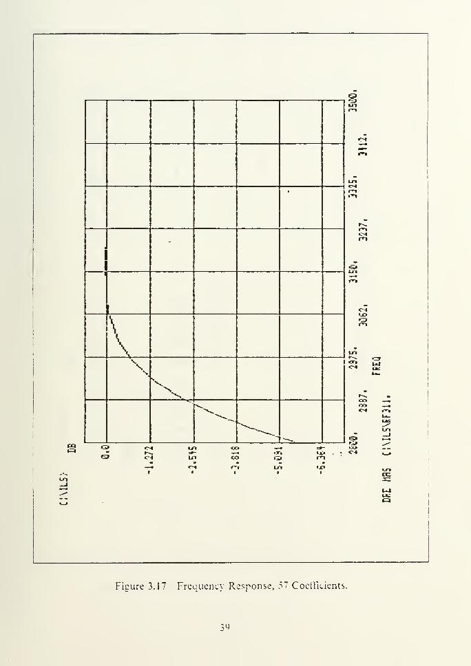
3.17 Frequency Response, 57 Coefficients 39
3.18 Frequency Response, 41 Coefficients 40
3.19 Frequency Response, 41 Coefficients 41
3.20 Sampled Data File, DF100 44
3.21 Sampled Data File, DF101 45
3.22 Plot of the Sequences of (a) and (b) 46
3.23 DFT of Sequence (a) , Af = 1 Hz 48
3.24 DFT of Sequence (b) , Af = 1 Hz 49
3.25 Sequences of Problem 2 [Ref 3: p. 482] 50
3.26 Sampled Data File WD100 51
3.27 Sampled Data File WD 101 51
3.28 Record Data WD 200 and WD201 53
3.29 Record Data, Xj(n) * x2(n) 55
3.30 Record Data, x,(n) * x2(n) 56
3.31 FORTRAN Program to generate samples 57
3.32 Sampled Data from FORTRAN Program 58
3.33 ILS Record Data from WRTIN.DAT 59
3.34 Input Data part (a) 60
3.35 Input Data part (b) 61
3.36 DFT Coefficients part (a) 62
3.37 DFT Coefficients part (a) 64
3.38 DFT Coefficients part (b) 65
I. DIGITAL SIGNAL PROCESSING SOFTWARE
A. INTRODUCTION
The purpose of this study is to evaluate the Interactive Laboratory Systems
(ILS-PC) digital signal processing software package. This is accomplished in three
ways. First, by identifying the need for digital signal processing software and the basic
computational operations that a software package of this type should perform.
Secondly, by describing the operation of the software and development of a conceptual
thought process that incorporates ILS in solving digital signal processing problems.
Finally, by using ILS to solve a number of problems and evaluating the software
package by comparing its capabilities and limitations with existing tools available for
digital signal processing at the Naval Postgraduate School.
B. NEED FOR DIGITAL SIGNAL PROCESSING SOFTWARE
As modern technology tends more toward digital methods in signal processing
and analysis, the need for software that consolidates and decreases the computational
burden of these methods becomes apparent. Time savings are realized if the software
is interactive and requires only input parameters. From an academic perspective, use
of this software can improve instructional effectiveness and increase the research
productivity of students. Solutions that require redundant computations such as, for
example, determining the frequency response of a filter, can be completed without
substantial programing. This increases the flexibility and availability of computer
generated solutions for analysis. Finally, use of this software helps the student remain
abreast of available analysis tools.
C. DIGITAL SIGNAL PROCESSING SOFTWARE PACKAGEREQUIREMENTS
1. Personal Computer Based Software
The first requirement is for the software to be compatible with personal
computers. While the obvious trade off between this and a mainframe installation is a
loss in computational precision and available memory, there are a number of
advantages. The most important advantage is the flexibility and portability of personal
computers. First, the user can purchase the software commercially. This eliminates
dependence upon software packages only available on the mainframe system. Using

personal computers eliminates the user's need to transfer programs between different
computer systems and the compatibility adjustments to the programs that may be
encountered in doing this. Personal computers can also be upgraded as necessary to
meet the individual needs oi" the user. This presents the potential for the creation of a
tailored library of signal processing programs.
Of equal importance is availability and cost savings when compared to a
mainframe system. A personal computer based system is subject to the user's schedule.
Unlike a mainframe system, there is no competition for CPU time or unavailability due
to scheduled maintenance and unscheduled down times. Also, there is no need to buy
computer time.
2. Signal Processing Capabilities
The requirements for a signal processing software package depend on its
intended use, however, there are some basic capabilities that will be needed for all
situations. The software should be flexible enough to allow the user to obtain the
solution of most signal processing problems. The following requirements are intended
to be a basis of what is expected of a signal processing software package:
Interactive Interface. The software should allow the user to describe signals or
systems through the use of a keyboard or other interactive interface.
Signal Generation. There should be the capability to create or form
combinations of common sequences such as sinusoids, exponentials, samples, or
other similar sequences.
External Data Input. The software should accept input data from an external
source or disk file for analysis.
Graphical Output. The software should provide well-labeled graphical output
of signals or analysis results on both an interactive video screen or in hard copy
at the user's option.
Extendability. The software should allow the user to describe new operations
and add these to the system.
Time Domain Operations. The software should be able to perform commontime domain operations, such as convolution and filtering.
Frequency Domain Operations. The software should be able to perform
common frequency domain operations, such as radix 2 FFT and frequency
responses.
Random Signals. The software should be able to generate random signals with
user-specified characteristics.
Determination of Statistical Characteristics. The software should be able to
compute statistical characteristics of signals, such as probability density
functions, correlation functions, cross correlation, etc.
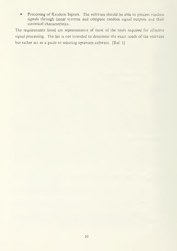
• Processing of Random Signals. The software should be able to process randomsignals through linear systems and compute random signal outputs and their
statistical characteristics.
The requirements listed are representative of most of the tools required for effective
signal processing. The list is not intended to determine the exact needs of the software
but rather act as a guide to selecting optimum software. [Ref. 1]
10
II. USING ILS
Having established the requirements for digital signal processing software, the
analysis of a software package can begin. Interactive Laboratory System (ILS-PC) was
purchased by the ECE department for this purpose. The scope of this analysis is to
describe the operation of ILS and from this develop a general process to facilitate using
the software. Initially, this evaluation of ILS was conducted using ILS version 5.0,
however, a newer version, ILS version 6.0, was acquired late in the development of this
study. To incorporate the improvements and changes of this new version, the version
6.0 capabilities are listed along with a discussion of the newer ILS menu mode of
operation.
A. DESCRIPTION OF ILS
ILS is a personal computer based digital signal processing tool. The software
can operate in two modes, the command line mode and the menu mode. The signal
processing functions that ILS performs can be summarized in eight areas. Discussion
of these topics reinforces the utility and capability of ILS as an independent signal
processing work station.
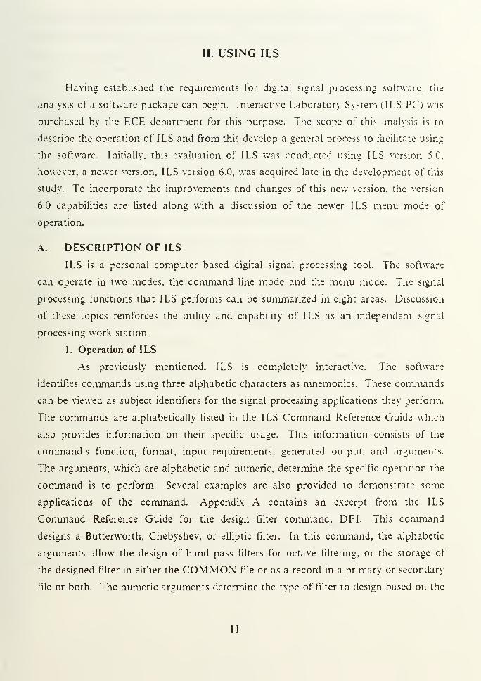
1. Operation of ILS
As previously mentioned, ILS is completely interactive. The software
identifies commands using three alphabetic characters as mnemonics. These commands
can be viewed as subject identifiers for the signal processing applications they perform.
The commands are alphabetically listed in the ILS Command Reference Guide which
also provides information on their specific usage. This information consists of the
command's function, format, input requirements, generated output, and arguments.
The arguments, which are alphabetic and numeric, determine the specific operation the
command is to perform. Several examples are also provided to demonstrate some
applications of the command. Appendix A contains an excerpt from the ILS
Command Reference Guide for the design filter command, DFI. This command
designs a Butterworth, Chebyshev, or elliptic filter. In this command, the alphabetic
arguments allow the design of band pass filters for octave filtering, or the storage of
the designed filter in either the COMMON file or as a record in a primary or secondary
file or both. The numeric arguments determine the type of filter to design based on the
11
user's specification of sampling frequency, stopband attenuation, passband attenuation,
band edges and the order of the filter. The output consists of very useful information
such as the pass band and stop band edges, the sampling frequency, the transfer
function of the filter, the poles and zeroes, and the first and second order quadratic
factors of the transfer function. [Ref. 2: p. 6-5]
The utility of this command is extensive, considering the many different types
of filters that can be designed; however, it is only a small part of the signal processing
analysis capability of ILS. Complete signal processing analysis with ILS requires the
successive use of different commands. For example, the frequency response of a filter
transfer function generated by the DFI command and stored in a record file can be
determined by using the Fast Fourier Transform (FFT) command. Successive
commands do not have to be related to the design process. Examples of this are the
List Records (LRE) command, which lists the contents stored in a record file and the
Display Records (DRE) command which graphically displays a record file on the
terminal screen.
a. Command Line Mode
The command line mode operation of ILS is meant for the experienced
user. Use of this mode requires the user to manipulate the ILS commands and their
arguments to perform the desired analysis. There are two ways to operate ILS in this
mode. The first method is to execute successive commands, applicable to the required
analysis, one command at a time, examining the intermediate results obtained by
performing each command. This gives the user an opportunity to inspect each part of
the analysis process, preventing the cascading of errors. The second method is
operation of the command line mode with a delimiter. This allows the user to enter a
number of commands on the command line to be performed as one command. This
gives the user an ability to perform repetitive analysis of a system much more
efficiently than with the first method. Since there are approximatly 90 ILS commands
to choose from, operation in this mode can become both tedious and time consuming.
A method which can simplify the selection of appropriate ILS commands for analysis
is the menu mode. [Ref. 2: pp. 6-1 and 7-7]
b. Menu Mode
The ILS menu mode is designed to help beginners to use ILS. There are
many menus that make up this mode. The menu structure is treelike, allowing the user
to make choices which narrow general categories until eventually data entry for a
12
particular signal processing application is performed. Each menu item has a function
key associated with it for selection. If ILS command argument entry is required, the
screen displays the arguments for data entry.
The menu mode of ILS operation has several advantages. First, there is no
need to open or create file space for the intermediate results of commands used in the
signal processing analysis; this is performed automatically. The menus narrow the
selection of ILS commands to choose from in terms of the desired signal processing
application. The obvious disadvantage of working with a menu driven system is having
to prompt through each of the menus for processes which require the redundant
selection of commands. Because of this, ILS allows the user to jump directly to a
specific menu using the direct access facility or between the menu mode and the
command line mode. This gives the user access to the advantages of both ILS
subsystems. [Ref. 2: p. 4-5]
2. Capabilities of ILS
The capabilities of ILS can be organized into eight categories. The following
is a list these categories and some of the functions available through the software.
1. Data input output. ILS allows the user to acquire and playback data through
A D and DA hardware, generate waveforms such as sinusoids, exponentials,
noise and speech, and convert data from external files in ASCII or binary
format into ILS format for analysis and reconvert to its original form for
transfer back.
2. Waveform Display. ILS can display data with a standard XY or three
dimensional plot. There are also options for overlay plotting and expanding of
segments of data for display.
3. Numeric Listing. ILS allows the user to list the numeric contents of datasets or
ILS files.
4. Data Manipulation and Editing. ILS allows the user to convert data between
coordinate systems, such as polar to rectangular, scale data through
multiplication or addition of an offset, modify particular points in a file, or shift
data to represent a delay.
5. Frequency Analysis. ILS allows the user to perform functions such as
computing a Fourier transform using a radix-2 FFT, coherence analysis to
generate normalized cross spectra, or transfer function estimation, which allows
the user to estimate a transfer function and review its Bode and Nyquist plot.
6. Digital Filtering. ILS allows the user to design recursive and non-recursive
filters, compute and graphically display their frequency responses, and allows
filtering of data through the designed filter for analysis.
13

7. Numerical Analysis. ILS allows the user to average, integrate or differentiate
data. Other applications include performing convolution, correlation and
waveform arithmetic.
8. Speech Processing. ILS allows the user to perform speech processing analysis
such as linear predictive coding analysis or pitch analysis. There are also
options to display and review speech data, spectra or vocal tracts. [Ref. 2: pp.
4-14 to 4-19]
3. Summary.
A general description of the operation and capabilities of ILS has been
presented. The signal processing commands in this package consists of a number of
self-contained programs. This is advantageous since it allows the user to execute a
series of these commands in performing signal processing analysis. Minimal
programming is required, since the ILS commands only require the input of arguments
which represent the problem parameters. The ILS commands are also general and
flexible enough to be tailored to almost any signal processing application.
B. GUIDE TO PROBLEM SOLVING WITH ILS
As with any application of a computer software package, a systematic approach
can be developed to facilitate the use of ILS. This process is best understood after a
review of general problem solving techniques.
1. Problem Solving Technique
The first requirement in solving any problem is to identify certain parameters.
It is essential to identify what is given, what needs to be determined, what are the
relationships pertinent to the problem, and what assumptions are to be made. Having
answered these questions, an ordered sequence of steps can be followed which leads to
the solution of the problem. This can involve many things such as simplifications of
equations or programming of redundant operations. The final step in the process is to
examine the results and determine their validity and acceptability as a solution.
2. Problem Solving Techniques With ILS
Determining solutions with ILS follows the same process, however, ILS limits
the analysis techniques available for signal processing. This requires the user to
manipulate ILS software to get a solution. The problem solving process with ILS is
summarized as follows:
1. Determine what is given or available in the problem statement.
2. Identify from the problem statement what must be determined.
14
3. Identify what ILS commands would be useful in solution of the problem. This
is more easily accomplished using the ILS menu mode.
4. Order the ILS commands required in solution of the problem.
5. Execute the commands of part (4) and examine the results. Repeat steps 3-5 as
necessary until the solution is satisfactory.
This process is short due to the interactive structure of ILS. It also allows the user to
experiment and determine an optimal solution.
C. PROBLEM SOLVING WITH ILS
1. ILS Files
With ILS, the use of successive commands in the analysis process produces a
requirement for storage of intermediate results in files. ILS works through the
manipulation of these files. ILS files are also used to store data input from an external
circuit and data transfered from other computer files. The type of data stored in a file
determines the type of file it is and there are five different types of data. File
manipulation and generation are the basis for successfully using ILS.
a. COMMON File
The COMMON file is required at all operating levels of ILS. storing
information to interface and operate the software such as parameter definitions,
constants, and status flags. Changes to the contents of the COMMON file are by
default written over the previous contents allowing for automatic updating of system
parameters. Since this file is always read first when booting ILS, the user always starts
exactly where the previous session ended. The COMMON file also has the utility of
being a scratch pad for storage of intermediate results. Data from the COMMON file
can be extracted and manipulated by transfering it to an ILS applicable type of file
using appropriate ILS commands. [Ref. 2: p. 6-2]
b. Other Files
The following is a list of other files internal to ILS:
1. Sampled Data Files. Data for these files is always in integer format and is
created using any of three ILS data sources:
• Test Signals and Functions. ILS has commands that need output files to
store their results. These commands generate sampled data files by
sampling ILS generated waveforms created by the user.
• External Files. ILS can be used to create data files from external files in
ASCII format, coded ASCII format, or binary format. This allows the user
to input data that can be analyzed using ILS commands. There are
requirements for the format of the external data. The ILS CommandReference Guide contains the pertinent details of these conditions.
15

• Analog Waveform. ILS has the capability of accepting an analog source as
input to create a data file. With ILS compatible A D and DA hardware,
the software can convert external signals to ILS format for analysis. This
is not explored by this thesis. [Ref. 2: p. 8-8]
2. Analysis Files. Analysis files store data created by executing speech analysis
programs on segments of sampled data. The data is integer data in vector form.
3. Record Files. Record files can store two types of data. The first type is signal
processing data. These data consist of real or complex points and is
representative of a time or Fourier series. The second type is feature data,
which is a matrix or vector representation of properties of experimental data.
4. Label Files. Label files store label data which is ASCII data describing in code
and words the location of significant events or segments in sampled data files.
[Ref. 2: p. 6-3]
2. Using ILS Files
Binary files are the files that ILS uses the most. These files are the sampled
data files, record files and analysis files. All of these files are structured the same. The
lengths of the ILS files are set by the user and only limited by the available memory on
the disk used. The length is expressed in disk blocks, 512 bytes per block. The file
blocks are numbered from U to N-l, where N is the number of blocks in a file. The
ILS command, FIL, is used to create, delete, select, or unprotect a file. The details of
the use of this command are contained in the ILS Command Reference Guide and are
demonstrated in the next chapter. An important point in using ILS files is how they
are selected and identified. ILS files are identified by two alphabetic characters and a
file number (1 - 9998). The two letter prefix is used to represent a single file or a group
of files. Each ILS file may be selected with one of six different pointers. These
pointers are primary A, B, or C, and secondary A, B, or C. Which pointers to use
depends on how the file is used by ILS commands. This is best explained by the
following example in which two time series record data files are convolved using the
Convolution (CXV) command. According to the command requirements, one file must
be declared a Primary (A) file and the other a Primary (B) file; however, a Secondary
(A) file must also be opened in order to store the results. In this case the FIL
command must be used three times, first to declare one file as primary (A), second to
declare the other file as Primary (B), and finally to declare a file as secondary (A) to
store the results. This allows the user to save the original data for further analysis, if
desired. For instance, the file declared the Primary (B) file could be redesignated the
Primary (C) file and the contents altered. The file can then be redesignated as the
16
Primary- B file and the convolution performed again. It makes the files easy to use,
however, keeping track of the files and what each contains may become a problem.
More detailed examples to help understand the use of ILS files will be presented in the
following chapter. [Ref. 2: pp. 8-3 to 8-5]
17
III. SOLVING PROBLEMS WITH ILS
The purpose of the following examples is to demonstrate the use of ILS in digital
signal processing. The problems show in detail the terminal input and output of
running the ILS commands in the command line mode and outline the use o[ the
problem solving techniques developed in Chapter II. The format that ILS commands
require is outlined in Chapter 6 of reference (2). The meanings of the command
arguments are outlined in the ILS Command Reference Guide.
A. DIGITAL FILTER DESIGN
The following three examples display different methods of using ILS to design
recursive and non-recursive digital filters.
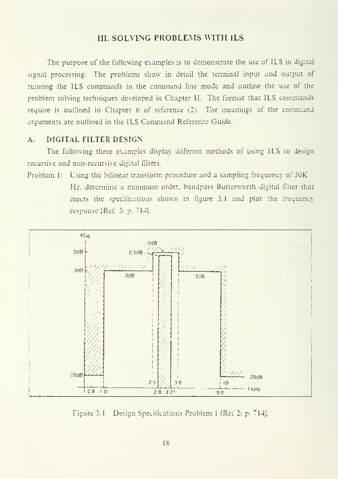
Problem 1: Using the bilinear transform procedure and a sampling frequency of 50K
Hz. determine a minimum order, bandpass Butterworth digital filter that
meets the specifications shown in figure 3.1 and plot the frequency
response [Ref. 3: p. 714].
M.rtB
OdB
3dB
/////
'///
'///A
W/A
Y/ /.
OdB K ''
' < <
08 10
OdB
5dB-^A-5-
3dB
2 5
/ / -
/
V/
/A
• Y//
3dB
36
28 321
/V
V,/
'/'/
/' /
'/'
/
I
V,Y// 20dBi 10
90— I kHz
Figure 3.1 Design Specifications Problem 1 [Ref 2: p. 714].
18
The analysis begins with determining what is given in the problem statement that
can help in designing the filter. In this problem, the given information includes the
sampling frequency of the filter and the stopband. cutoff and passband attenuations
and frequencies for the filter. The next step is to determine what must be found to plot
the frequency response. This requires determining the order of the filter and the
transfer function. The third step is to determine what ILS commands are to be used in
the the solution of the problem. The following ILS commands apply:
File Command (FIL). This command is used to list, select, create, unprotect, or
delete a file.
Open Record File Command (OPN). This command is used to create and
initialize primary and secondary files.
Design Filter Command (DFI). This command is used to design an elliptic,
Butterworth, or Chebyshev filter.
List Records Command (LRE). This command lists signal processing records
from consecutive primary or secondary files.
Fast Fourier Transform Command (FFT). This command is used to perform
Fast Fourier Transform operations on records.
Display Record Command (DRE). This command is used to display signal
processing record files.
In this problem, the FIL and OPN commands must be used first to create storage for
the record data that will be generated using the DFI and FFT commands. Next, the
DFI command is used to determine the transfer function of the filter. The FFT
command is then used to determine the frequency response and DRE displays the
results. The LRE command can be used any time during the analysis to list the record
data generated by DFI or FFT. The order in which the ILS commands are used is as
follows:
1. Initialize two files to store the results of the DFI and FFT commands. This
is done using the FIL command with the DEY argument which deletes any data
in the file TQ100. The first numeric argument is the numerical filename of the
file and the second is the number of consecutive files to delete starting with
TQ100. ILS will by default make file TQ100 the primary (A) file.
Input: FIL DEYTQ100„2
ILS responds with: TQ100. DOES NOT EXIST
TQ101. DOES NOT EXIST
TQ100. DOES NOT EXIST
PRIMARY FILE
19
2. The files are prepared to accept data. The DFI command can store the
transfer function of the filter as a record in the COMMON file or a primary or
secondary file. If the transfer function of the filter is stored as a record in the
COMMON file, only the Frequency Display (FDI) command can be used to
compute and display the frequency response. This command automatically
scales the display but does not produce a numerical listing of the frequency
response thereby limiting the user to relying on the display to interpret how
closely the filter meets design specifications. To obtain a numerical listing of
the frequency response, the FFT command must be used. This commanu
requires that the filter's transfer function (the results of the DFI command) be
stored as a record in a primary file. The file TQ100 is initialized as a record file
and opened to accept record data by the OPN command.
Input: OPN
ILS responds with: (A system prompt.)
3. The DFI command is executed by entering the command with its arguments.
The values of the arguments are determined using the design specifications of
the problem. The order of the filter was determined to be two using non ILS
techniques. For this problem, the P argument allows the filter to stored as a
record. The first numeric argument is the order of the Filter and the second is
the passband ripple in milli-dB and must be to indicate this is a Butterworth
filter. The third argument is the integer sampling frequency in Hz, the fourth
and fifth are the integer lower and upper band edges of the band pass filter.
The sixth argument is the stop band edge or "dB down" and must be for
Butterworth Filters. The last argument is the power of ten multiplier for the
frequencies.
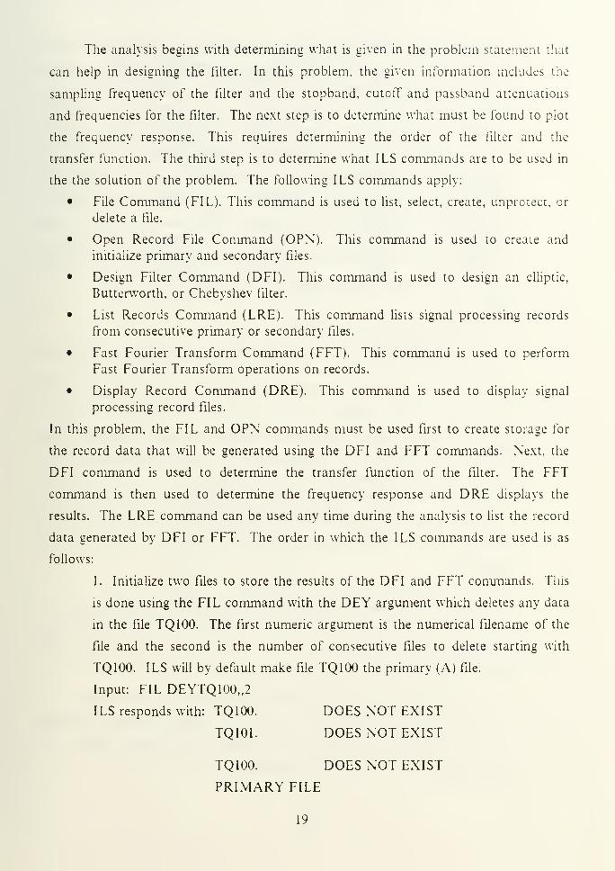
Input: DFI P2,0,500,25,36,0,2
ILS responds with: Figure 3.2, a listing of the transfer function of the filter.
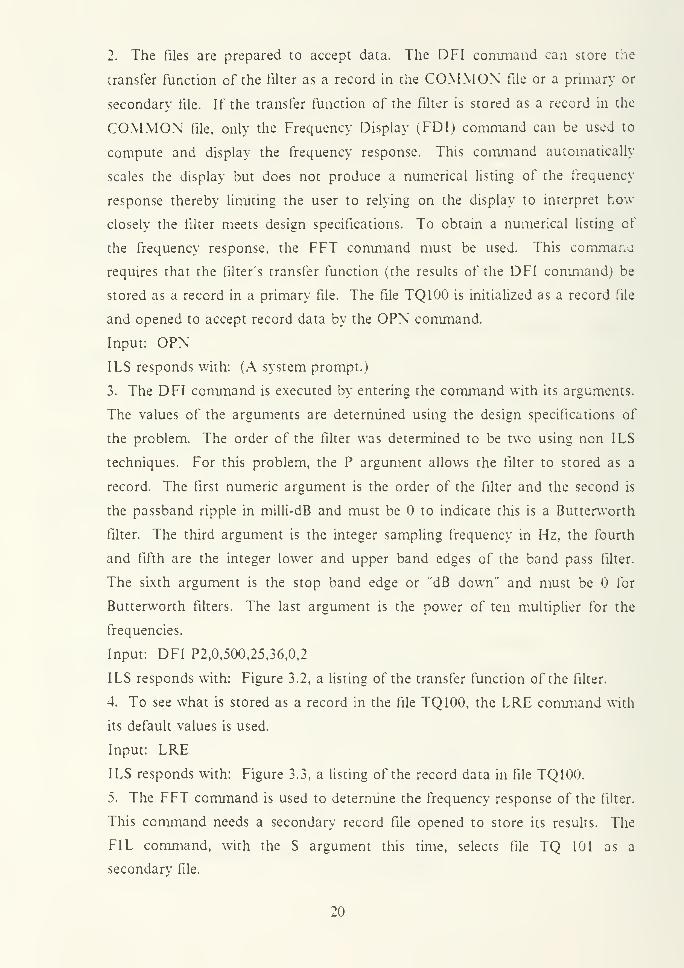
4. To see what is stored as a record in the file TQ100, the LRE command with
its default values is used.
Input: LRE
ILS responds with: Figure 3.3, a listing of the record data in file TQ100.
5. The FFT command is used to determine the frequency response of the filter.
This command needs a secondary record file opened to store its results. The
FIL command, with the S argument this time, selects file TQ 101 as a
secondarv file.
20
'
SAMPLING FREQUENCY 50000. 000 HZBND oaSS BUTTERwORTH ( f*«X I "rft_LY
"-AT) FILTER
BAND ED3C5
DENOMINATOR
£500. 000
NUMERATOR
3£oO. 000 nZ
1 1 . OOOOOOE+OO h. 346069E-032 -3. 537423E+00 . 00OOuuE*Ou3 4. 9<»0204E +00 -8. 692176E-034 .-3. 2O7272E+0O . OOOOOOE+005 8.224354E-01 4. 346083E-03
POLES QUADRATIC FACTORSREAL IMAGINARY FIRST ORDER SECOND ORDER
.361813 . 391486 -1. 723626 . 895964
. 306898 . 308949 -1.813796 . 917314ZEROS QUADRATIC FACTCR5
REAL IMAGINARY FIRST ORDER SECOND ORDER-l.OOOOOO . OOOOOO 1 . OOOOOO . OOOOOO1. 000000 . OOOOOO -1. OOOOOO . OOOOOO
-1. 000000 . OOOOOO 1 . OOOOOO . OOOOOO1. oooooo . OOOOOO -1 . OOOOOO . OOOOOO
TIME CONSTANT 23.350 SAMPLESNO IS £ BANDWIDTH 1218. 451 HZ
Figure 3.2 Output of DFI Command.
C: MLS) i_ RE
• C:\ILS\TQ100. 100, 1 RECORDS »
RECORD 1, SAMPLING FREQUENCY 5. 00E*04, TYPE 1121
REAL TIME SERIES OF FILTER COEFFICIENTS
INDEX NUMERATOR DENOMINATOR
1 4.3461E-03 l.OOOOE+OO2 . OOOOE+00 -3. 5374E+003 -8.69££E-03 4. 9402E+004 . OOOOE*00 -3. 2073£*005 *.3461E-03 8.2244E-01
EMTE3 C TO CONTINUE, E TO EXIT, N FOR NEXT RECORD->CRECORD 2 NOT FOUND
Tigure 3.3 Tile TQlUO, Record Data.
Input: F1L S1Q101
iLS responds with: TQ101. DOFS NOT FXIST
SECONDARY FILE
21
6. The OPX command is used as before to initialize TQ101 as a record file.
The S argument must be used since TQ101 is a secondary file.
Input: OPN S
ILS responds with: (A system prompt.)
7. The FFT command is executed to determine the frequency response. Since
the primary file contains the filter's transfer function, the command determines
the frequency response of the filter by dividing the FFT of the numerator by the
FFT of the denominator. By default, the order of the FFT used in each case, is
the smallest that contains all data points and the record is automatically zero
padded to bring it to the size of the FFT used. The arguments used with this
command are P, which stores the FFT in polar format, and 9, which specifies
that 29 = 512 points are to be used.
Input: FFT P„9
ILS responds with: TQ 101. RECORD 1 STORED
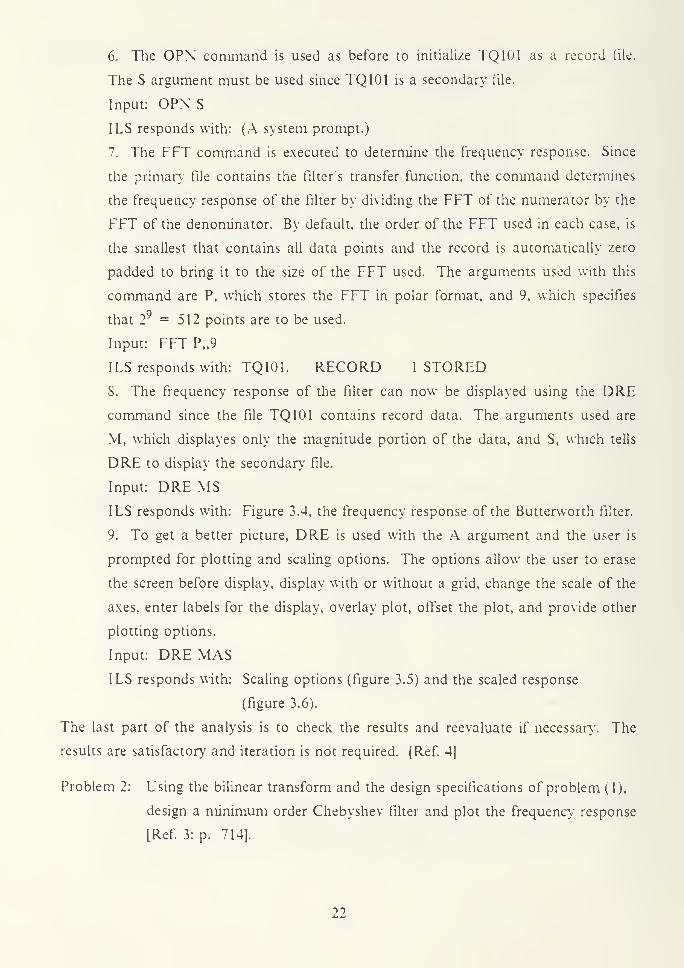
8. The frequency response of the filter can now be displayed using the DRE
command since the file TQ101 contains record data. The arguments used are
VI, which displayes only the magnitude portion of the data, and S, which tells
DRE to display the secondary file.
Input: DRE MS
ILS responds with: Figure 3.4, the frequency response of the Butterworth filter.
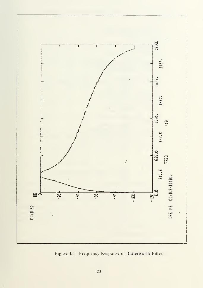
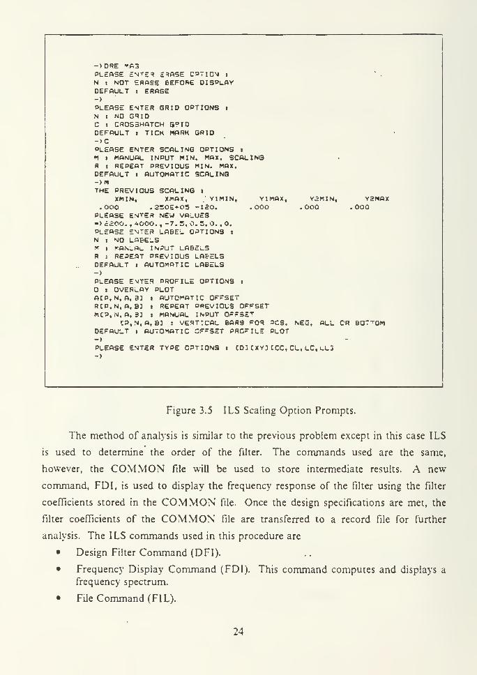
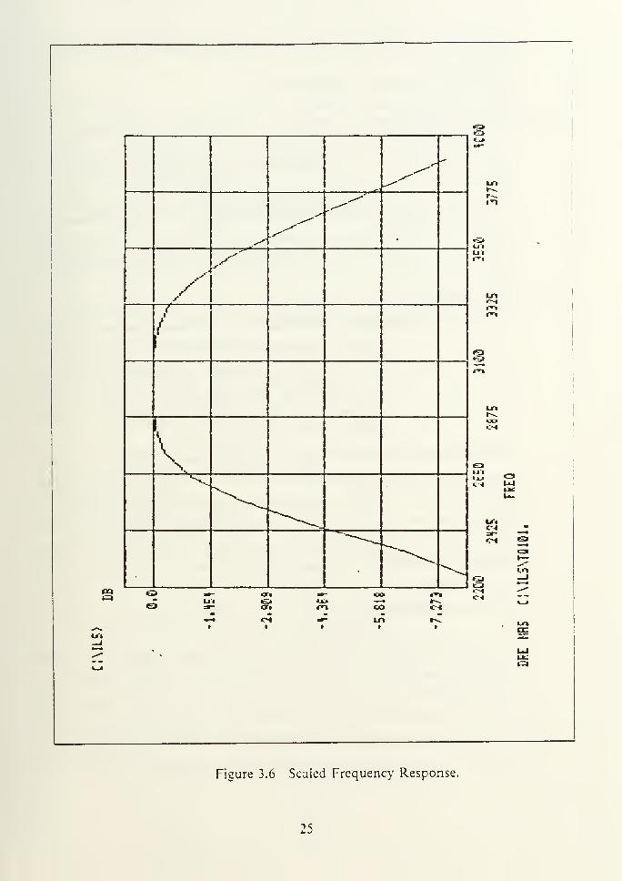
9. To get a better picture, DRE is used with the A argument and the user is
prompted for plotting and scaling options. The options allow the user to erase
the screen before display, display with or without a grid, change the scale of the
axes, enter labels for the display, overlay plot, offset the plot, and provide other
plotting options.
Input: DRE MASILS responds with: Scaling options (figure 3.5) and the scaled response
(figure 3.6).
The last part of the analysis is to check the results and reevaluate if necessary. The
results are satisfactory and iteration is not required. [Ref. 4]
Problem 2: Using the bilinear transform and the design specifications of problem (1),
design a minimum order Chebyshev filter and plot the frequency response
[Ref. 3: p. 714].
•>•>
6) K*>CO CO1 t
en
(=1
Figure 3.4 Frequency Response of Butterworth Filter.
23
->DRE *.fl3
PLEASE ENT£R E3ASE CPTION i"
.
N t NOT EROSE BEFORE DISPLAYDEFAULT i ERASE-)
PLEASE ENTER GRID OPTIONS I
N i NO GRIDC « CROSSHATCH Q?IDDEFAULT t TICK MARK GRID->CPLEASE ENTER SCALING OPTIONS I
M i MANUAL INPUT MIN. MAX. SCALINGR t REPEAT PREVIOUS MIN. MAX.DEFAULT i AUTOMATIC SCALING->MTHE PREVIOUS SCALING I
XMIN, XMAX, .* Y1MIN, V1MAX, Y.2MIN, Y2MAX.000 . 2S0E+05 -120. .000 .000 .000PLEASE ENTER NEW VALUES-> c£00. , AOOO. , -7. 5, 0. S, O. , 0.
PLEOSE ENTER LABEL OPTIONS I
N i NO L3BELS« » MANLAu INPUT LABELSR : REPEAT PREVIOUS LABELSDEFAULT t AUTOMATIC LABELS->
PLEASE EvJTER PROFILE OPTIONS I
O « OVERLAY PLOTACP, N, A, 33 l AUTOMATIC OFFSETRCP.N, A, B3 « REPEAT PREVIOUS OFFSETMCP.N, A, 33 i MANUAL INPUT 0FF3ET
CP, N,A, B3 : VERTICAL BARS ^OR 3CS, NEG, ALL CR BOTTOMDEFAULT » AUTOMATIC OF-SET PRG~ILE PLOT->
PLEASE ENTER TYPE OPTIONS I CD
j
CXY3 CCC, CL, LC, uLj->
Figure 3.5 ILS Scaling Option Prompts.
The method of analysis is similar to the previous problem except in this case ILS
is used to determine the order of the filter. The commands used are the same,
however, the COMMON file will be used to store intermediate results. A new
command, FDI, is used to display the frequency response of the filter using the filter
coefficients stored in the COMMON file. Once the design specifications are met, the
filter coefficients of the COMMON file are transferred to a record file for further
analysis. The ILS commands used in this procedure are
• Design Filter Command (DFI).
• Frequency Display Command (FDI). This command computes and displays a
frequency spectrum.
• File Command (FIL).
24
VV
ii
LJ t
1J I
Lit
in
He
C--I
CI Q
Ti
<-5
CO c^
1=1
Figure 3.6 Scaled Frequency Response.
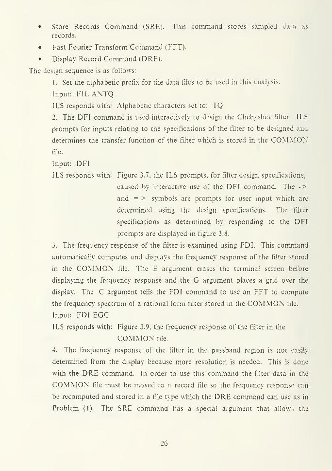
• Store Records Command (SRE). This command stores sampled data as
records.
• Fast Fourier Transform Command (FFT).
• Display Record Command (DRE).
The design sequence is as follows:
1. Set the alphabetic prefix for the data files to be used in this analysis.
Input: FILAXTQ
ILS responds with: Alphabetic characters set to: TQ
2. The DFI command is used interactively to design the Chebyshev filter. ILS
prompts for inputs relating to the specifications of the filter to be designed and
determines the transfer function of the filter which is stored in the COMMONfile.
Input: DFI
ILS responds with: Figure 3.7, the ILS prompts, for filter design specifications,
caused by interactive use of the DFI command. The ->
and = > symbols are prompts for user input which are
determined using the design specifications. The filter
specifications as determined by responding to the DFI
prompts are displayed in figure 3.8.
3. The frequency response of the filter is examined using FDI. This command
automatically computes and displays the frequency response of the filter stored
in the COMMON file. The E argument erases the terminal screen before
displaying the frequency response and the G argument places a grid over the
display. The C argument tells the FDI command to use an FFT to compute
the frequency spectrum of a rational form filter stored in the COMMON file.
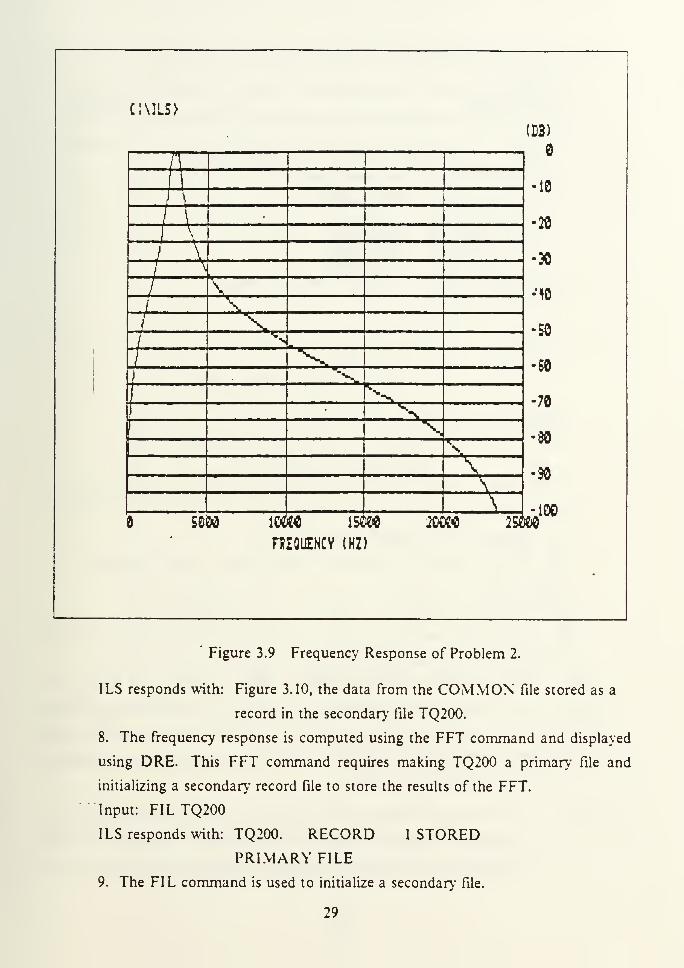
Input: FDI EGC
ILS responds with: Figure 3.9, the frequency response of the filter in the
COMMON file.
4. The frequency response of the filter in the passband region is not easily
determined from the display because more resolution is needed. This is done
with the DRE command. In order to use this command the filter data in the
COMMON file must be moved to a record file so the frequency response can
be recomputed and stored in a file type which the DRE command can use as in
Problem (1). The SRE command has a special argument that allows the
26

C:\ILS>D-I
1 - L0W-JQS3, 2 - BOND-PASS, 3 - HIGHPA55, 4 - BAND-REJECTPLEASE EnTEiR NUMBER->2
ENTER SAMPLE FREQUENCY, PASS BAND EDGE(S) (FLT PT)-> 50000. ,100 2800. ,3210.
ENTER S'OP BAND EDGE, ONLY ONE MAY BE USER SPECIFIED,EVEN WHEN FILTER IS PASS BAND OR STOP BAND (FLT PT)-> 1000.
STOP BAND EDGE(S) 1000.00 8337.94
TRPNSITION RATI0»19.Ee, THETfl- 2.37
ENTER PASS BAND VARIATION (MILLIDB), AND STOP BQND ATTENUATION <DB) (FLT PT)UITh CHEBYCHEV AND ELLIPTIC FILTERS THERE WILL BE RIPPLES IN THEPASS BAND. WITH THE ELLIPTIC AND CHEBYChEV II THERE WILL BERIPPLES IN THE STOP BAND. DB DEFAULTS TO 3.0103 DB.
PLEASE EmTER THE TWO REQUESTED NUMBERS (FLT PT)=») 500. , £0.MINIMUM PROTOTYPE ORDER REQUIRED (NOTE TmQT FOR THE DIGITAL PASS BANDCR S"Q3 3AND FILTERS, THIS WILL BE DOUBLED)
t
BUTTERWCRTH 1.1, CHEBYCnEV 1.1, ELLIPTIC 1.1
ENTER ORDER OF PROTOTYPE FILTER YOU WISH TO USE-> 2
ENTER NUMBER TO INDICATE WHICH PARAMETER TO CHANGE1 = STOP BAND EDGE, 2 - DB ATTENUATION-> 1
?Q=5 F<o\D £D3E(S) 2800.0 3210.0BUTTERWCRTH HALF POWER POINT (S) 2670.7 326'*. 1
STOP BAND EDGE(S) ELLIPTIC 2309.8 3879.3STOP BAND EDGS(S) CHEBYCHEVS .0 .OSTOP BAND EDGE(S) BUTTERWORTH £093.1 4268.1
THE FOLLOWING LIST THE ENTRIES YOU C0UL2 '^KE DIRECTLY ON THECOMMAND _INE TO DESIGN THE FILTERS AND AvjID ANY PROMPTING
DFI 2. O, 5OO0, 267. 226. O -) BU'^ERWORTHDF
I
£, 500, 5000, 281.1. 3i: 1
.
-> C-tEBYCnEVDFI i, 0. SOOQ, O. 0, -20 -> CHEBYCHEV TYPE II
DFI 2, 5O0, 5000, 26u, 321, -20 -) Et_i_IPT"IC
EiSiTER "lu'ER "YPE TO USEf'-E PRC3RAn „;^_ ENTER 7Ai_'_ES FOR YOU):
1 =» BUT-'ERWJT'H, 2 = CHEDVC-IV, 2 - INVERTED CHEBYCHEV, 4 ELLIPTIC
Figure 3.7 DTI S\stcm Prompts.
27
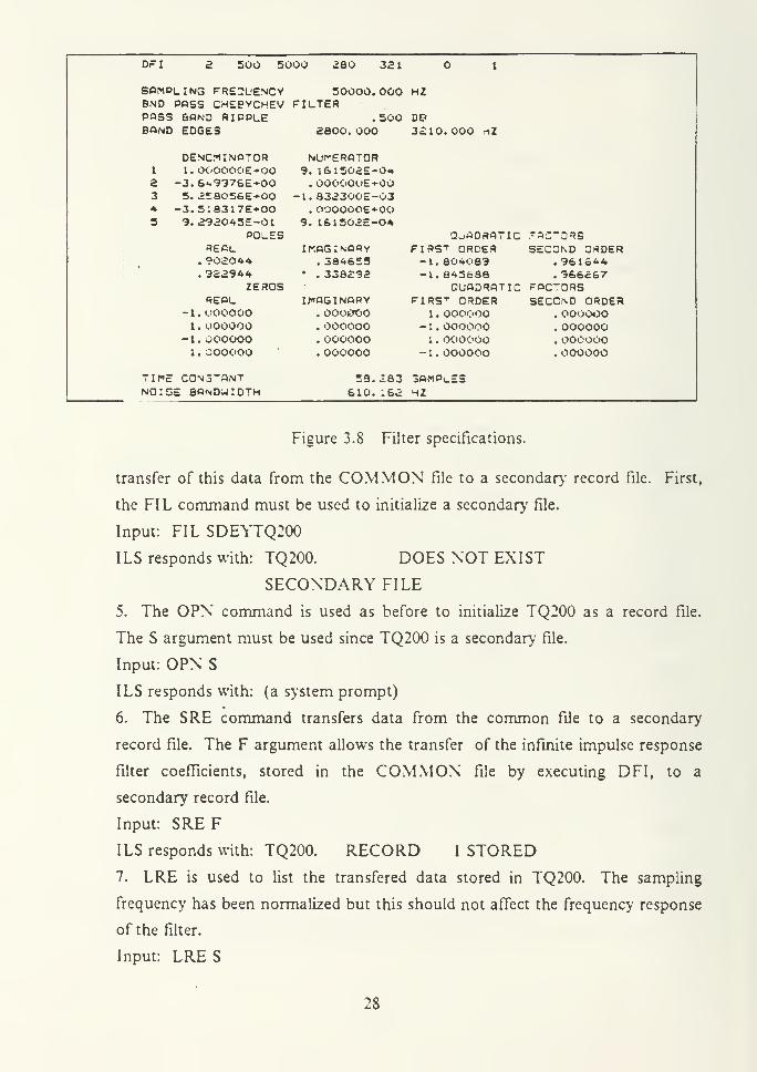
Dr I 2 500 5000 280 321 1
SPMPLING FREQUENCY 50000. 000 HZBND 30SS CHEPYCHEV FILTERPQSS BOND RIPPLE .500 DBBOND EDGES
DENCniNOTOR
2800. 000
NUfEROTOR
3210.000 HZ
1 1. OOOOOOE+00 9. 161502E-042 -3.6^9376E*00 . OOOOOuEfOO3 5. 258056E+00 -1 . 8323OOE-034 -3. 5:8317Ei-00 . OOOOOOE+OOS 9. 293045E-01 9. 161502E-O4
POLES QoODROTIC .-ocroRsREOt_ I cog; NOR
Y
FIRST ORDER SECOND ORDER. 902044 . 384655 -1. 804083 . 9616^4. 322944 • . 338292 -1. 845688 . 966267
ZEROS QUODROTIC DOCTORSREPL IfiOGINQRY FIRST ORDER SECOND ORDER
-1. OOOOOO . OOOOOO i . ooo<:>oo . OOOOOOI . OOOOOO . OOOOOO - 1 . OOOOOO . OOOOOO
-1.000000 . OOOOOO 1 . OOOOOO . OOOOOO1. OOOOOO . OOOOOO -1. OOOOOO . OOOOOO
7ir"E C0\"ONT 58.183 30MPi_ESNOISE BONDuiIDTH 610. 162 HZ
Figure 3.8 Filter specifications.
transfer of this data from the COMMON file to a secondary record file. First,
the FIL command must be used to initialize a secondary file.
Input: FIL SDEYTQ200
I LS responds with: TQ200. DOES NOT EXIST
SECONDARY FILE
5. The OPN command is used as before to initialize TQ200 as a record file.
The S argument must be used since TQ200 is a secondary file.
Input: OPN S
ILS responds with: (a system prompt)
6. The SRE command transfers data from the common file to a secondary
record file. The F argument allows the transfer of the infinite impulse response
filter coefficients, stored in the COMMON file by executing DFI, to a
secondary record file.
Input: SRE F
ILS responds with: TQ200. RECORD 1 STORED7. LRE is used to list the transfered data stored in TQ200. The sampling
frequency has been normalized but this should not affect the frequency response
of the filter.
Input: LRE S
28
c:\ils>
1
1
)
1 \
\
i
\
/ \
i*
/ \/ v
f\
/ N -
I \I
•--^-v
"sV\\
\
:sb)
e
•to
•20
•30
•10
-50
•60
•70
•80
•30
sm m$ \sm 2occ« iszw
FiEOUENCV (H2)
•100
' Figure 3.9 Frequency Response of Problem 2.
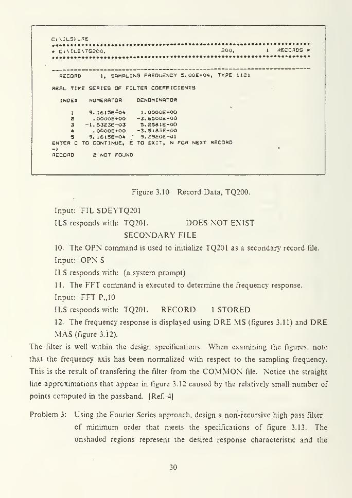
ILS responds with: Figure 3.10, the data from the COMMON file stored as a
record in the secondary file TQ200.
8. The frequency response is computed using the FFT command and displayed
using DRE. This FFT command requires making TQ200 a primary file and
initializing a secondary record file to store the results of the FFT.
Input: FILTQ200
ILS responds with: TQ200. RECORD I STORED
PRIMARY FILE
9. The FIL command is used to initialize a secondary file.
29
C« MLS) L3E
» C« \ILS\TG200. 200, 1 RECORDS »
RECORD 1, SAMPLING FREQUENCY 5. 00E+04, TYPE 11£1
REAL TIME SERIES OF FILTER COEFFICIENTS •
INDEX NUMERATOR DENOMINATOR
1 9. 1615E-0* 1 . 000OE-M3O2 . OOOOE+OO -3. 6500E+003 -1.8323E-03 3.2581E+0O4 . OOOOE+OO -3. 5183E+003 9. J6X5E-04 ; 9.292OE-01
ENTER C TO CONTINUE, E->
RECORD 2 NOT FOUND
TO EXIT, N FOR NEXT RECORD>
Figure 3.10 Record Data, TQ200.
Input: FIL SDEYTQ201
ILS responds with: TQ201. DOES NOT EXIST
SECONDARY FILE
10. The OPN command is used to initialize TQ201 as a secondary record file.
Input: OPN S
ILS responds with: (a system prompt)
1 1. The FFT command is executed to determine the frequency response.
Input: FFT P„10
ILS responds with: TQ201. RECORD 1 STORED
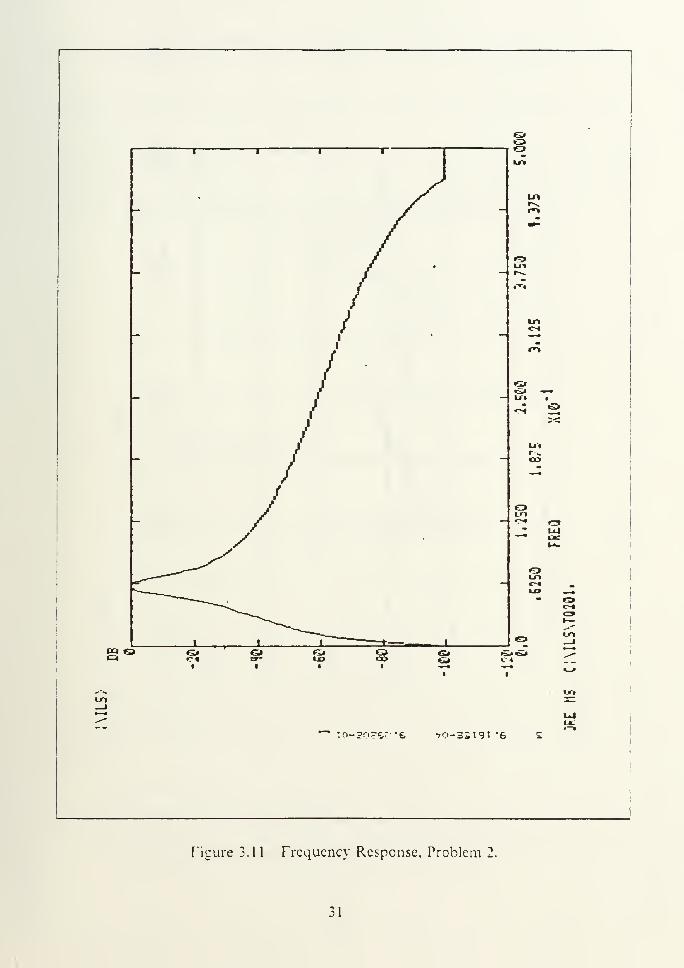
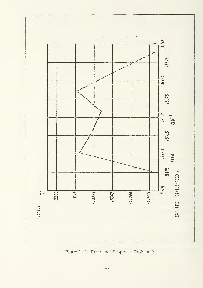
12. The frequency response is displayed using DRE MS (figures 3.11) and DREMAS (figure 3.12).
The filter is well within the design specifications. When examining the figures, note
that the frequency axis has been normalized with respect to the sampling frequency.
This is the result of transfering the filter from the COMMON file. Notice the straight
line approximations that appear in figure 3.12 caused by the relatively small number of
points computed in the passband. [Ref. 4]
Problem 3: Using the Fourier Series approach, design a non-recursive high pass filter
of minimum order that meets the specifications of figure 3.13. The
unshaded regions represent the desired response characteristic and the
30
Si
SIf • 1 r
• in
t
S»in
-
j
/1
f
•
inC-*
-
/S»
/f ui
CO
- /f S»
— peu-
1 I I i
1
SIin
s» _,
s ei Si•
Si•
S»COi
Sis»
•5c>s» ^1 :-.
:0-30?&^*6 *>0-3ST9T "6
figure 3.11 Frequency Response, Problem 2.
31
CQ
N
>V
r--.
in
«£3 im •
u* e>• XblC-|o>Ui
oLO•x» r3in UJ• *"£
l»-
ini
—
se*- _^in «5>• <--«
c=»*—-^in
«s»G* .—
•
»s»
Q - ^r*i r*» «x>
**~~ • • • •ITI
VXl
_^~ UIUe
•_» i=a
Figure 3.12 Frequency Response, Problem 2.
o
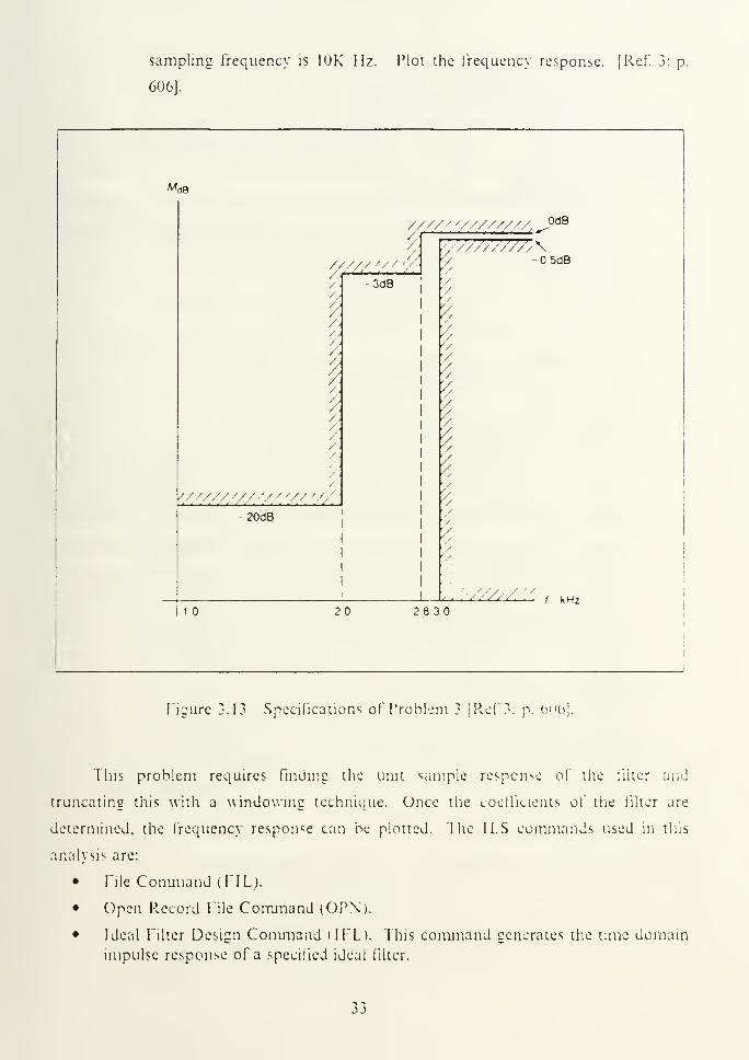
sampling frequency is 10K Hz. Plot the frequency response. [Ref. 3: p.
606].
Md3
'" ——_^—
,
///// '///////A _-0<jB
% />//////Zv\y - 5dB
//////////// >
-3dB V/
''A
!
/
/
.
/
1
/
.
t/ • •/
1
//////////// '/''// ''
/'/20dB' /
1'/
i
'/1
1
1i
1
1
i
i
1 2 2 8 3
i
Figure 3.13 Specifications of Problem 3 [Ref 3': p. 6»>6].
This problem requires finding the unit sample response of the filter and
truncating this with a windowing technique. Once the coefficients of the filter are
determined, the frequency response can be plotted. The ILS commands used in tins
analysis are:
• rile Command (FIL).
• Open Record file Command (OPN).
• Ideal Filter Design Command (IFF). This command generates the tune domain
impulse response of a specified ideal filter.
33
• Fast Fourier Transform Command (FFT).
• Display Records Command (DRE).
The IFL command is used to determine the coefficients of the filter. The FFT
command determines the frequency response using the filter coefficients. The design
sequence is as follows:
1. Set the alphabetic prefix for the data files to be used in this analysis, create a
file to store the record generated by the IFL command and open the file to
accept record data.
Input: FIL AXRFI LS responds with: Alphabetic characters set to: RF
Input: FIL DEYRF300
ILS responds with: RF300. DOES NOT EXIST
PRIMARY FILE
Input: OPN
ILS responds with: (a system prompt)
2. The IFL command is used to determine the coefficients of the filter. This is
done by using an FFT and the user specified spectral characteristics of the ideal
filter. The first argument of the command is the order of the FFT for the
design. The second, third and fourth are the integer sampling, lower cutoff and
upper cutoff frequencies of the filter. The fifth is the power often multiplier for
the frequencies, the sixth is the number of filter points to output and the
seventh is the window type to use in the analysis. In the first trial of the design
process, 31 coefficients are determined and a Hamming window is used by
default.
Input: IFL 9,10000,2800,5000,0,31
ILS responds with: RF300. RECORD 1 STORED
3. A secondary file is created and opened to store the record data that will be
generated by determining the frequency spectrum of the filter using the FFT
command.
Input: FIL SDEYRF301
ILS responds with: RF301. DOES NOT EXIST
SECONDARY FILE
Input: OPN S
ILS responds with: (a system prompt)
4. The FFT command is used to determine the frequency response.
34
Input: FFT P.. 10
I LS responds with: RF301. RECORD 1 STORED
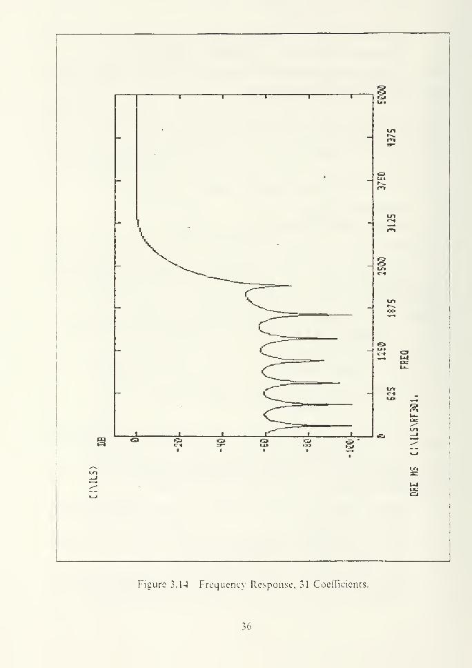
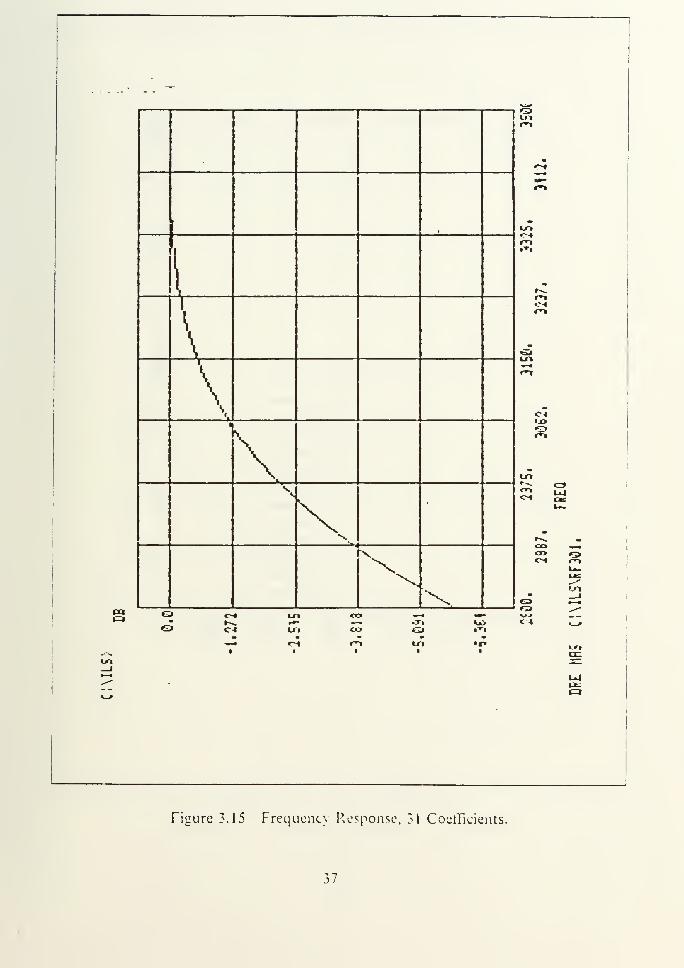
5. The frequency response is displayed using the DRE MS (figure 3.14) and
DRE MAS (figure 3.15) commands.
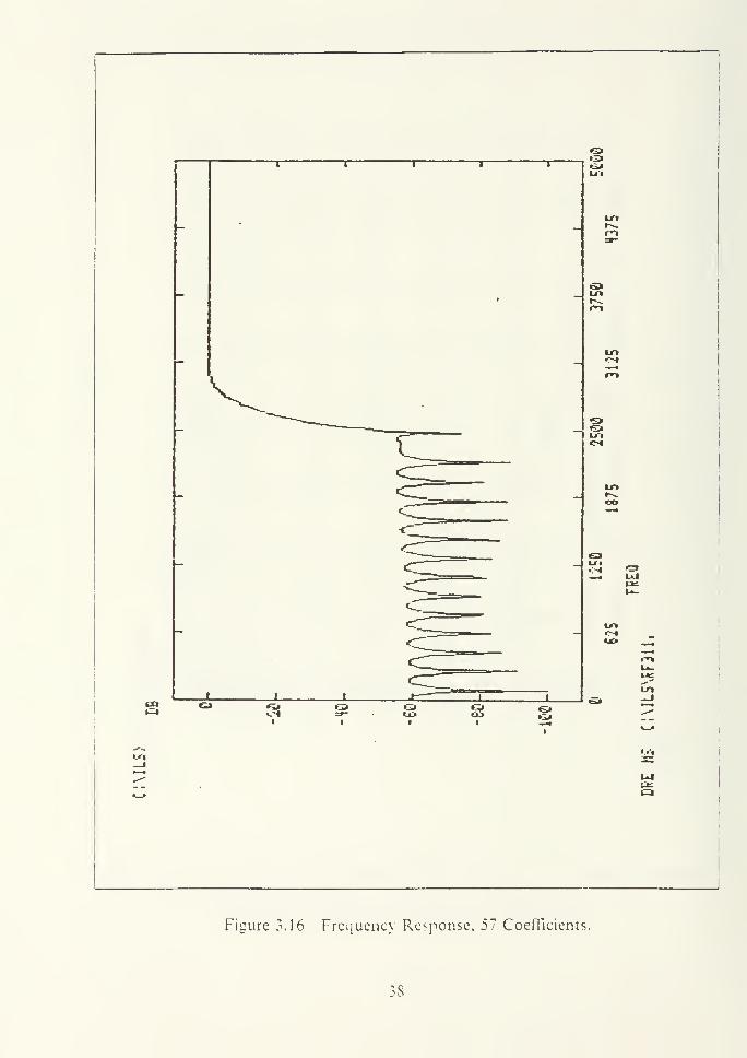
The filter does not meet the design specifications with 31 coefficients. After further
iterations the specifications are meet using a filter of 57 coefficients (figures 3.10 and
3.17). This design uses more coefficients than necessary since the -3 dB cutoff
frequency is approximately 2S75 Hz and only 2SU0 Hz is required. Decreasing the
cutoff frequency, the order of the filter can be further reduced. The final filter has an
order of 41 coefficients (figures 3.18 and 3.19). [Ref. 4]
B. SPECTRAL ANALYSIS
In the following examples ILS will be used to perform spectral analysis. In the
fist problem, ILS is used to compute the DFT of two finite sequences. In the second
problem ILS is used to perform the convolution of two sequences. The last problem is
also a DFT computation, however, the data for the sequence are input using an
external data file.
Problem 4: Find the discrete Fourier transform for each of the following 40-point
sequences [Ref 2: p. 486]:
a) x (n) = 1, n = 0, 1, 39
x (n) = 0, otherwise
b) x (n) = 1, n = 0, 1, 2, 3, 37, 38, 39
x (n) = 0, otherwiseP '
In this problem ILS must be used to create the sequences and then find their
DFTs. The commands to be used are:
Context Command (CTX). This command lists or changes the context (number
points per frame), sector number, or header length of a file.
File Command (FIL).
Initialize Command (INA). This command initializes or changes the primary
sampled data file header.
Modify Command (MDF). This command modifies the values of the sampled
data or signal processing record data.
Print Command (PRT). This command prints sampled data.
Display Command (DSP). This command displays a time series waveform on
the screen.
33
• *~i
i
tni
c:\i
Figure 3.14 Frequency Response, 31 Coefficients.
36
\1
\1
\1
\\
X
\
<~4
LTD
U4
G» c~» in co• l-^. s*- <W4
G» C-4 LTI CO
-—
•
r~i n«-!>
•^
fa
1 — r~i m in *£• 1Ul.--.. • t • i ccin -••
_i•—
•
UJ***Ut;
~ • n•_»
figure 3.15 Frequency Response, 31 Coefficients.
37
to1=1
Figure 3.16 Frequency Response. 57 CoelTicients.
•>••
38
\
\A *
\
"S.N.
Oui
in
C-l(Xt
CO
» J «--t w CO _<• »-^ ^- •«_ •T.Q C-4 Ln CO • il
•~+ c-» r»i 1/1
* *5i-»
Figure 3.17 Frequency Response, 57 Coeiikients.
39
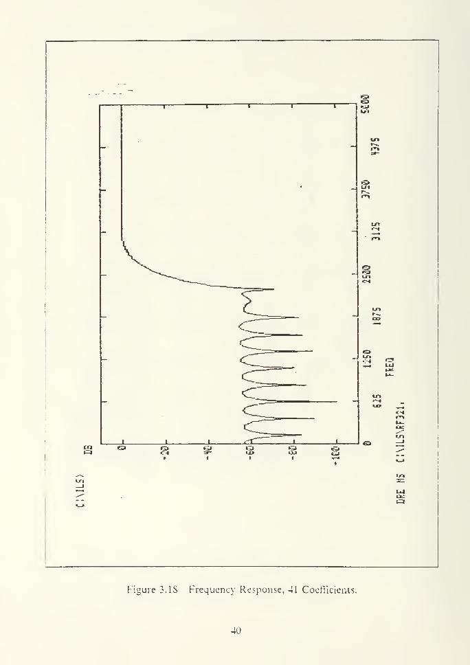
Figure 3.18 Frequency Response, 41 Coefficients.
40
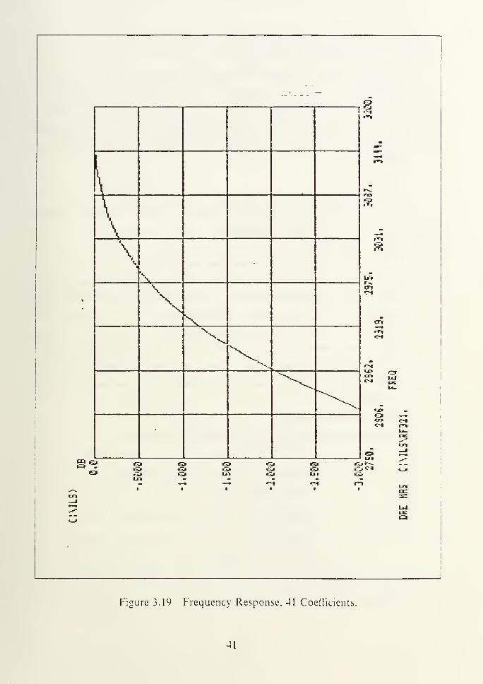
Figure 3.19 Frequency Response, 41 Coefficients.
41

• Frequency Display Command (FDI).
The sequence of the analysis is as follows:
1. The number of points per frame that a sampled data file contains is
designated by the CTX command. In this problem, the sequences are
40-points. FDI determines the DFT of a sampled data file by frame and
therefore, to obtain a DFT with no discontinuities the context, of the sampled
data files must be set to 40-points per frame, the implicit period of the
sequence.
Input: CTX 40
ILS responds with: CONTEXT = 40 POINTS; FRAME2. The prefix of the data files to be used in the analysis is initialized using the
FIL command with the AN argument.
Input: FIL ANDFILS responds with: Alphabetic characters set to: DF
3. The FIL command is used to create a file of 40 zeros. The first argument,
CRZ, creates a file filled with zeros. The numeric arguments of the command
determine the size and number of files created. The first argument is the
filename and filename numeric which identifies the primary file, the second
declares the number of files to create and the third declares the number of
frames per file to create. In this problem, two files are created each with one
frame. Only one filename numeric is entered since ILS sequentially numbers
the second file.
Input: FIL CRZDF100„2,1
ILS responds with: DF100. NOT SAMPLED DATA2 DK BLKS
DF101. NOT SAMPLED DATA2DK BLKS
DF100. NOT SAMPLED DATA2 DK BLKS
PRIMARY FILE
4. In order for this file to be sampled data, a sampling frequency must be
assigned to the file. ILS commands do not perform analysis with files unless a
file type is declared. For example, assigning a sampling frequency makes the
42
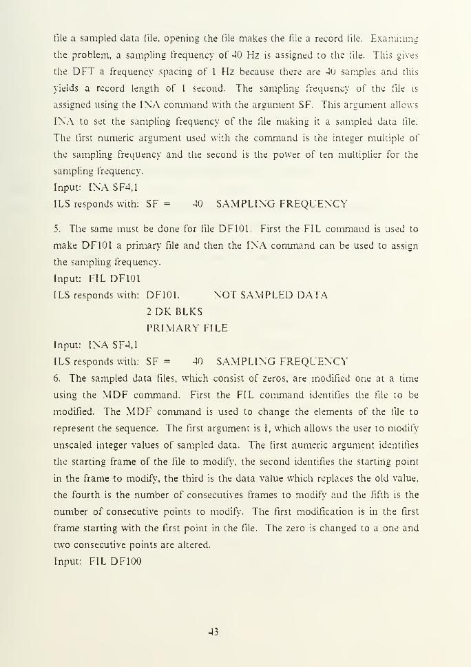
file a sampled data file, opening the file makes the file a record file. Examining
the problem, a sampling frequency of 40 Hz is assigned to the file. This gives
the DFT a frequency spacing of 1 Hz because there are 40 samples and this
yields a record length of 1 second. The sampling frequency of the file is
assigned using the INA command with the argument SF. This argument allows
INA to set the sampling frequency of the file making it a sampled data file.
The first numeric argument used with the command is the integer multiple of
the sampling frequency and the second is the power of ten multiplier for the
sampling frequency.
Input: INA SF4.1
ILS responds with: SF = 40 SAMPLING FREQUENCY
5. The same must be done for file DF101. First the FIL command is used to
make DF101 a primary file and then the INA command can be used to assign
the sampling frequency.
Input: FIL DF101
ILS responds with: DF101. NOT SAMPLED DATA2 DK BLKS
PRIMARY FILE
Input: INA SF4,1
ILS responds with: SF = 40 SAMPLING FREQUENCY6. The sampled data files, which consist of zeros, are modified one at a time
using the MDF command. First the FIL command identifies the file to be
modified. The MDF command is used to change the elements of the file to
represent the sequence. The first argument is I, which allows the user to modify
unsealed integer values of sampled data. The first numeric argument identifies
the starting frame of the file to modify, the second identifies the starting point
in the frame to modify, the third is the data value which replaces the old value,
the fourth is the number of consecutives frames to modify and the fifth is the
number of consecutive points to modify. The first modification is in the first
frame starting with the first point in the file. The zero is changed to a one and
two consecutive points are altered.
Input: FIL DF100
43
ILS responds with: FIL DF100. SAMPLED DATA
2 DK BLKS. 1. FRAMES, 40 PT FR
SAMPLE RATE = 40 HZ
PRIMARY FILE
Input: MDF 11,1.1.1,2
ILS responds with: OLD = 0, NEW = 1
Input: MDF 11.40.1.1.1
ILS responds with: OLD = 0, NEW = 1
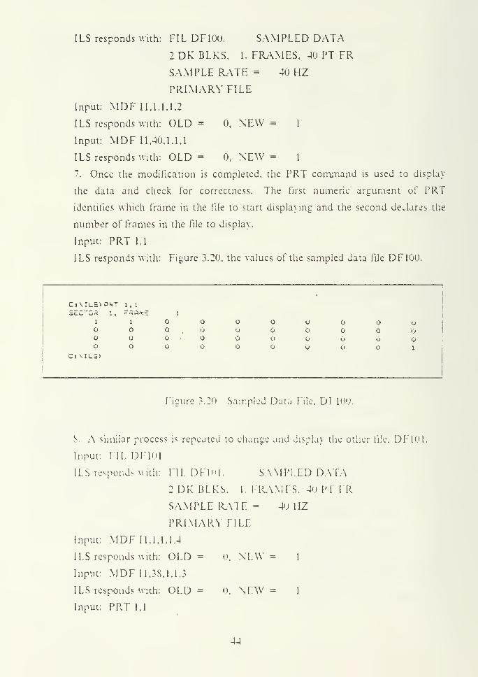
7. Once the modification is completed, the PRT command is used to display
the data and cheek for correctness. The first numeric argument of PRT
identifies which frame in the file to start displaying and the second declares the
number of frames in the file to display.
Input: PRT 1,1
ILS responds with: Figure 3.20, the values of the sampled data file DF100.
Ci \n_s> put 1. 1
•
3C.L ^ <uR I , r rTA.TI'I 1
1 1 oo O o O
O o O oo O 1
C: \IL=>
Figure 3.20 Sampled Data File. DITOO.
S. A similar process is repeated to change and display the other file. DF10I
Input: ML DF101
ILS responds with: FIL DF101. SAMPLED DATA
2 DK BLKS. I. FRAMES. 4(J Pi FR
SAMPLE RATE = 40 HZ
PRIMARY FILE
Input: MDF 11.1,1.1.4
ILS responds with: OLD = 0, NEW = 1
Input: MDF 11.38.1.1.3
ILS responds with: OLD = 0. NEW = 1
Input: PRT 1.1
44
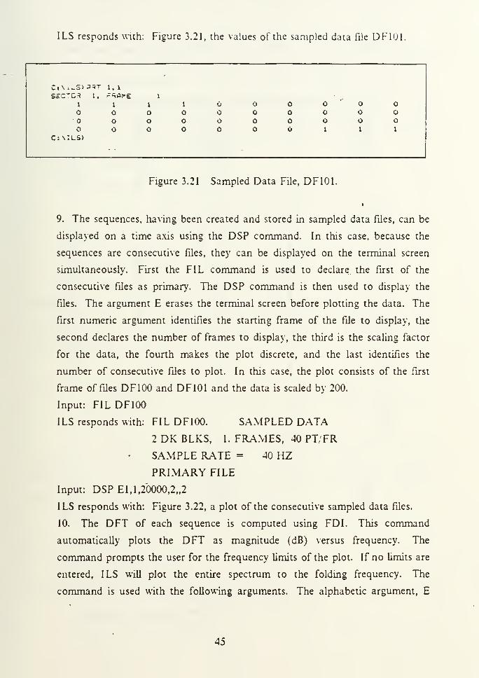
ILS responds with: Figure 3.21, the values of the sampled data file DF1U1,
Ci\iwS> P *T 1. 1
SECTD3 1. r=»A|r£ 1
I 1 1 1
O o• o o o
1 I 1
C:\ILS)-
Figure 3.21 Sampled Data File, DF101.
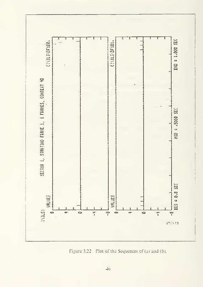
9. The sequences, having been created and stored in sampled data files, can be
displayed on a time axis using the DSP command. In this case, because the
sequences are consecutive files, they can be displayed on the terminal screen
simultaneously. First the FIL command is used to declare the first of the
consecutive files as primary. The DSP command is then used to display the
files. The argument E erases the terminal screen before plotting the data. The
first numeric argument identifies the starting frame of the file to display, the
second declares the number of frames to display, the third is the scaling factor
for the data, the fourth makes the plot discrete, and the last identifies the
number of consecutive files to plot. In this case, the plot consists of the first
frame of files DF100 and DF101 and the data is scaled by 200.
Input: FIL DF100
ILS responds with: FIL DF10O. SAMPLED DATA
2 DK BLKS, 1. FRAMES, 40 PT/FR
SAMPLE RATE = 40 HZ
PRIMARY FILE
Input: DSP El,l,20000,2„2
ILS responds with: Figure 3.22, a plot of the consecutive sampled data files.
10. The DFT of each sequence is computed using FDI. This command
automatically plots the DFT as magnitude (dB) versus frequency. The
command prompts the user for the frequency limits of the plot. If no limits are
entered, ILS will plot the entire spectrum to the folding frequency. The
command is used with the following arguments. The alphabetic argument, E
45
l—i—
r
cr:
L3
U-l
I I I L
t—i—
r
I ota
J I »
i—i—
r
i i i
i—i—
r
QO
II
Krt
Ul
II
•1*
I I LCXI COI
: \ 3
Figure 3.22 Plot of the Sequences of (a) and (b).
46
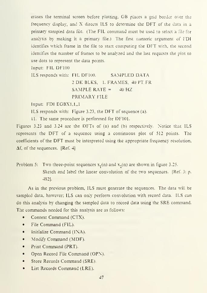
erases the terminal screen before plotting. GB places a grid border over the
frequency display, and X directs ILS to determine the DFT of the data in a
primary sampled data file. (The FIL command must be used to select a file for
analysis by making it a primary' file.) The first numeric argument ol' FDI
identifies which frame in the file to start computing the DFT with, the second
identifies the number of frames to be analyzed and the last requests the plot to
use dots to represent the data points.
Input: FIL DF100
ILS responds with: FIL DF100. SAMPLED DATA2 DK BLKS, 1. FRAMES, 40 PT/FR
SAMPLE RATE = 40 HZ
PRIMARY FILE
Input: FDI EGBX1,1„1
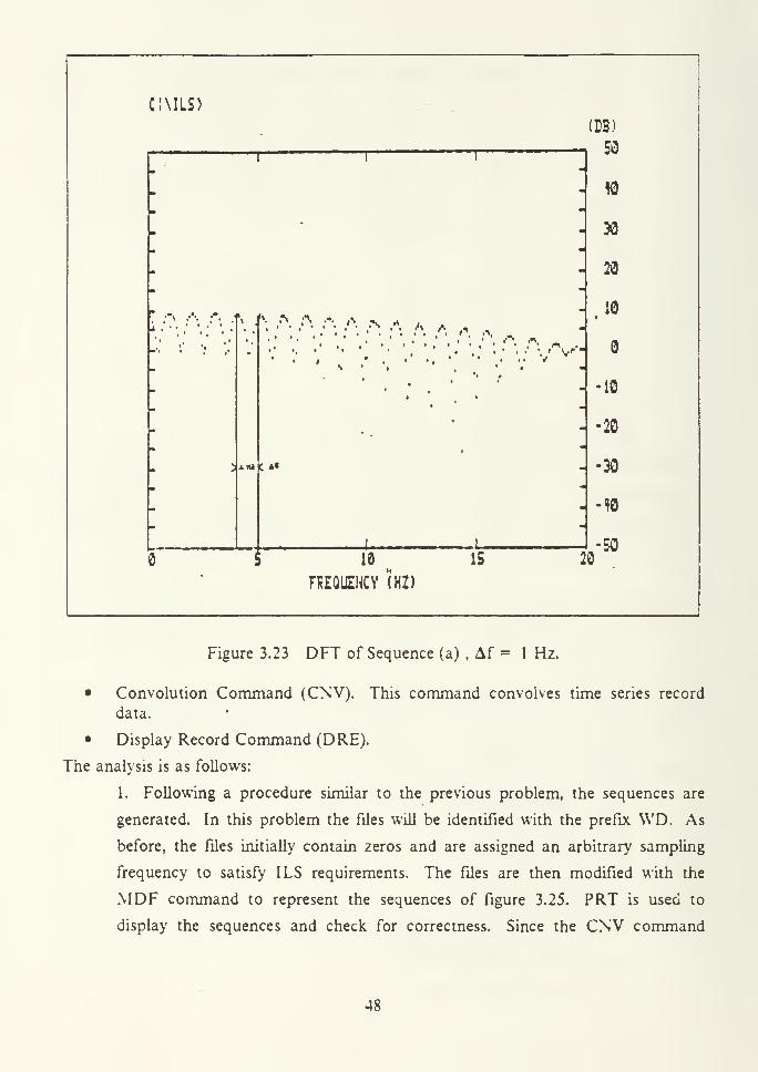
ILS responds with: Figure 3.23, the DFT of sequence (a).
1 1. The same procedure is performed for DF101.
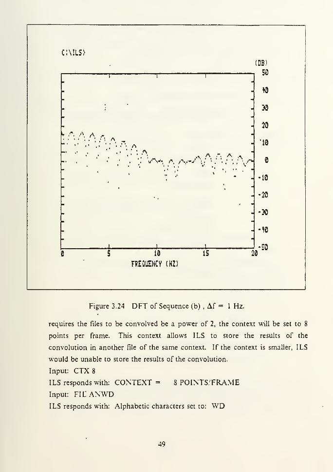
Figures 3.23 and 3.24 are the DFTs of (a) and (b) respectively. Notice that ILS
represents the DFT of a sequence using a continuous plot of 512 points. The
coefficients of the DFT must be interpreted using the appropriate frequency resolution,
Af, of the sequences. [Ref. 4]
Problem 5: Two three-point sequences Xj(n) and x2(n) are shown in figure 3.25.
Sketch and label the linear convolution of the two sequences. [Ref. 3: p.
482].
As in the previous problem, ILS must generate the sequences. The data will be
sampled data, however, ILS can only perform convolution with record data. ILS can
do this analysis by changing the sampled data to record data using the SRE command.
The commands needed for this analysis are as follows:
• Context Command (CTX).
• File Command (FIL).
• Initialize Command (I\A).
• Modify Command (MDF).
• Print Command (PRT).
• Open Record File Command (OPN).
• Store Records Command (SRE).
• List Records Command (LRE).
47
c:\ils>
• % A 1\ .^ a
) xm
•• ^ ' A A .*. A A />. ,n .,.'• , ....••.••.' • ' • :
n- n .
C *«
(DB)
50
W
30
20
10•
•10
•20
-30
MO
$ 10
FUZQUZHCV (HZ)
15 20
-50
Figure 3.23 DFT of Sequence (a) , Af = 1 Hz.
• Convolution Command (CNV). This command convolves time series record
data.
• Display Record Command (DRE).
The analysis is as follows:
1. Following a procedure similar to the previous problem, the sequences are
generated. In this problem the files will be identified with the prefix WD. As
before, the files initially contain zeros and are assigned an arbitrary sampling
frequency to satisfy ILS requirements. The files are then modified with the
MDF command to represent the sequences of figure 3.25. PRT is used to
display the sequences and check for correctness. Since the CNV command
48
c : \ils>
If *'••..'• <\ .
'• • ' .' '. .*»
.». A .". A ..
(SB)
50
W
30
20
'10
-10
•20
•30
•W
10
FT?EQLENCV (HZ)
15 20
-50
Figure 3.24 DFT of Sequence (b) , Af = 1 Hz.
requires the files to be convolved be a power of 2, the context will be set to 8
points per frame. This context allows ILS to store the results of the
convolution in another file of the same context. If the context is smaller, ILS
would be unable to store the results of the convolution.
Input: CTX8ILS responds with: CONTEXT = 8 POINTS/FRAME
Input: FIL'ANWD
ILS responds with: Alphabetic characters set to: WD
49
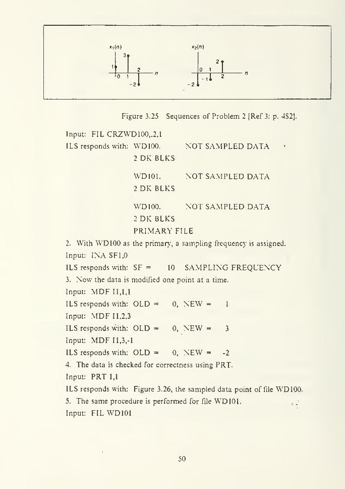
Figure 3.25 Sequences of Problem 2 [Ref 3: p. 482].
Input: FILCRZWD100„2,1
ILS responds with: WD 100. NOT SAMPLED DATA2 DK BLKS
WD101. NOT SAMPLED DATA2DK BLKS
WD 100. NOT SAMPLED DATA2DK BLKS
PRIMARY FILE
2. With WD 100 as the primary, a sampling frequency is assigned.
Input: INA SF 1,0
ILS responds with: SF = 10 SAMPLING FREQUENCY3. Now the data is modified one point at a time.
Input: MDF 11,1,1
ILS responds with: OLD = 0, NEW = 1
Input: MDF 11,2,3
ILS responds with: OLD = 0, NEW = 3
Input: MDF 11,3,-1
ILS responds with: OLD = 0, NEW = -2
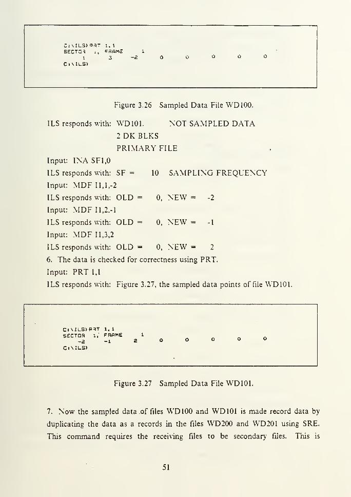
4. The data is checked for correctness using PRT.
Input: PRT 1,1
ILS responds with: Figure 3.26, the sampled data point of file WD100.
5. The same procedure is performed for file WD 101.
Input: FILWD101
50
C: \IL3> o*r I, \
SECTOR *, FSBME 1
1 5 -£ u o o
CiMlS)
Figure 3.26 Sampled Data File WD 100.
ILS responds with: WD 101. NOT SAMPLED DATA2 DK BLKS
PRIMARY FILE
Input: INA SF1.0
ILS responds with: SF = 10 SAMPLING FREQUENCYInput: MDF 11,1,-2
ILS responds with: OLD = 0, NEW = -2
Input: MDF 11,2.-1
ILS responds with: OLD = 0, NEW = -1
Input: MDF 11,3,2
ILS responds with: OLD = 0, NEW = 2
6. The data is checked for correctness using PRT.
Input: PRT 1,1
ILS responds with: Figure 3.27, the sampled data points of file WD101.
C» VluS>P*T 1, 1
SECTOR 1,' FRPWE-a -x
1o
CiMLS>
Figure 3.27 Sampled Data File WD 101.
7. Now the sampled data of Files WD100 and WD101 is made record data by
duplicating the data as a records in the Files WD200 and WD201 using SRE.
This command requires the receiving Files to be secondary files. This is
51
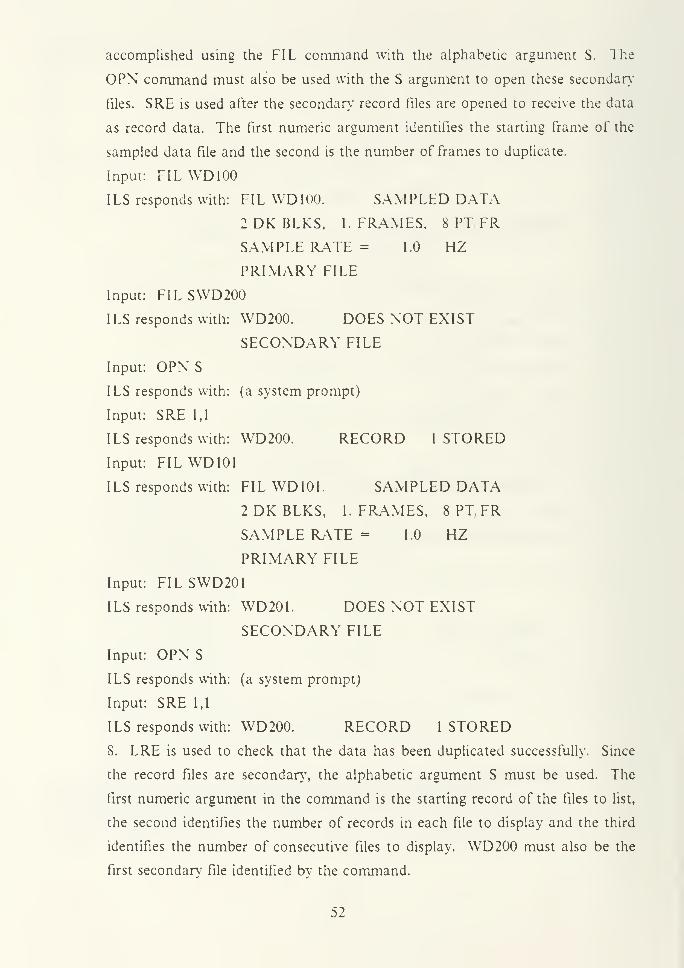
accomplished using the FIL command with the alphabetic argument S. The
OPN command must also he used with the S argument to open these secondary
files. SRE is used after the secondary- record files are opened to receive the data
as record data. The first numeric argument identifies the starting frame of the
sampled data file and the second is the number of frames to duplicate.
Input: FIL WD 100
ILS responds with: FIL VVD100. SAMPLED DATA
2 DK BLKS, 1. FRAMES, 8 PT FR
SAMPLE RATE = 1.0 HZ
PRIMARY FILE
Input: FIL SWD200
ILS responds with: WD 200. DOES NOT EXIST
SECONDARY FILE
Input: OPN S
ILS responds with: (a system prompt)
Input: SRE 1,1
ILS responds with: WD200. RECORD 1 STORED
Input: FIL WD 101
ILS responds with: FIL WD 101. SAMPLED DATA
2 DK BLKS, I. FRAMES, 8 PT, FR
SAMPLE RATE = 1.0 HZ
PRIMARY FILE
Input: FIL SWD201
ILS responds with: WD201. DOES NOT EXIST
SECONDARY FILE
Input: OPN S
ILS responds with: (a system prompt)
Input: SRE 1,1
ILS responds with: WD200. RECORD 1 STORED
8. LRE is used to check that the data has been duplicated successfully. Since
the record files are secondary, the alphabetic argument S must be used. The
first numeric argument in the command is the starting record of the files to list,
the second identifies the number of records in each file to display and the third
identifies the number of consecutive files to display. WD200 must also be the
first secondary file identified by the command.
52
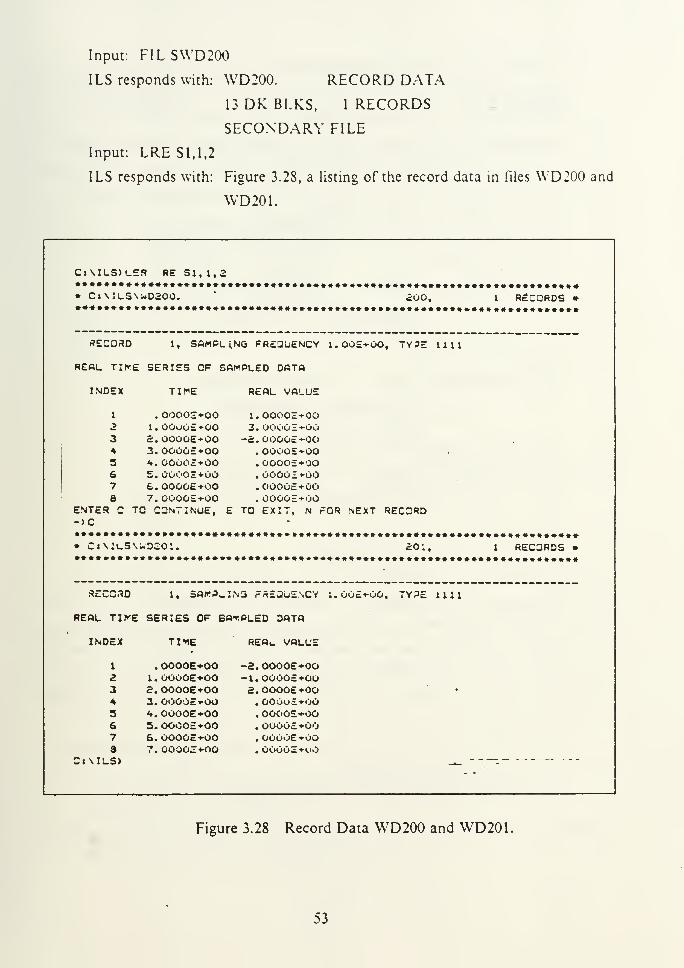
Input: FILSWD200
ILS responds with: WD200. RECORD DATA
13 DK BLKS, 1 RECORDS
SECONDARY FILE
Input: LRE SI, 1,2
ILS responds with: Figure 3.28, a listing of the record data in files WD200 and
WD201.
C»\ILS><_£ R RE SI, 1,2
» Ci\ILS\ -D200. 200, 1 RECORDS •
RECORD 1, SAMPLING FREQUENCY l.OOE+OO, TYPE 1111
REAL TIKE SERIES OF SAMPLED DATA
INDEX TIME REAL VALUE
I . OOOOE+OO 1. 00002*002 1. OOOOE+OO 3. OOOOE+OO3 2. OOOOE+OO -2. OOOOE+OO4 3. OOOOE+OO . OOOGS+003 4. OOOOE+OO . OOOOE+OO6 s. ogooe+oo . OOOOE+OO7 £. OOOOE+OO . OOOOE+OOB 7. OOOOE+OO . 0000£+00
ENTER C TO CONTINUE, E TO EXIT, N FOR NEXT RECORD->c •
• cj\ii_s\ud£o:. 201, 1 RECORDS •
accoao 1, SAMPLING FREQUENCY 1. OOE+OO, TYPE 1111
REAL TIKE SERIES OF SAMPLED DATA
INDEX TIME R£Ai_ VALUE
1 . OOOOE+OO -2. OOOOE+OO2 1. OOOOE+OO -I. OOOOE+OO3 2. OOOOE+OO 2. OOOOE+OO4 3. OOOOE+OO . OOGOE+003 <. OOOOE+OO .OOOOE+OO6 5. OOOOE+OO . OOOOE+OO7 6. OOOOE+OO . OOOOE+OOa 7. OOOOE+OO . OOOOE+OO
C«\ILS) '-V
Figure 3.28 Record Data WD 200 and WD201.
53

9. With the record files identified. CNV is used to perform convolution of the
two sequences. The CNV command requires one file to be a Primary (A) file
and the other to be a Primary (B) file. This is accomplished using the FIL
command. Default declares a file Primary (A) and the alphabetic argument B
declares a file Primary (B). CNV also requires a secondary file be opened to
store the results of the convolution. This is accomplished as before using the
FIL and OPN commands. WD 300 is used to store the results. None of the
CNV command's arguments are needed to perform the analysis.
Input: FIL WD200
ILS responds with: WD200. RECORD DATA13 DK BLKS, 1 RECORDS
PRIMARY FILE
Input: FIL BCV201
ILS responds with: WD201. RECORD DATA13 DK BLKS, 1 RECORDS
PRIMARY-B FILE
Input: FIL SWD300
ILS responds with: WD300. DOES NOT EXIST
SECONDARY FILE
Input: OPN S
ILS responds with: (a system prompt)
Input: CNV
ILS responds with: WD300. RECORD 1 STORED
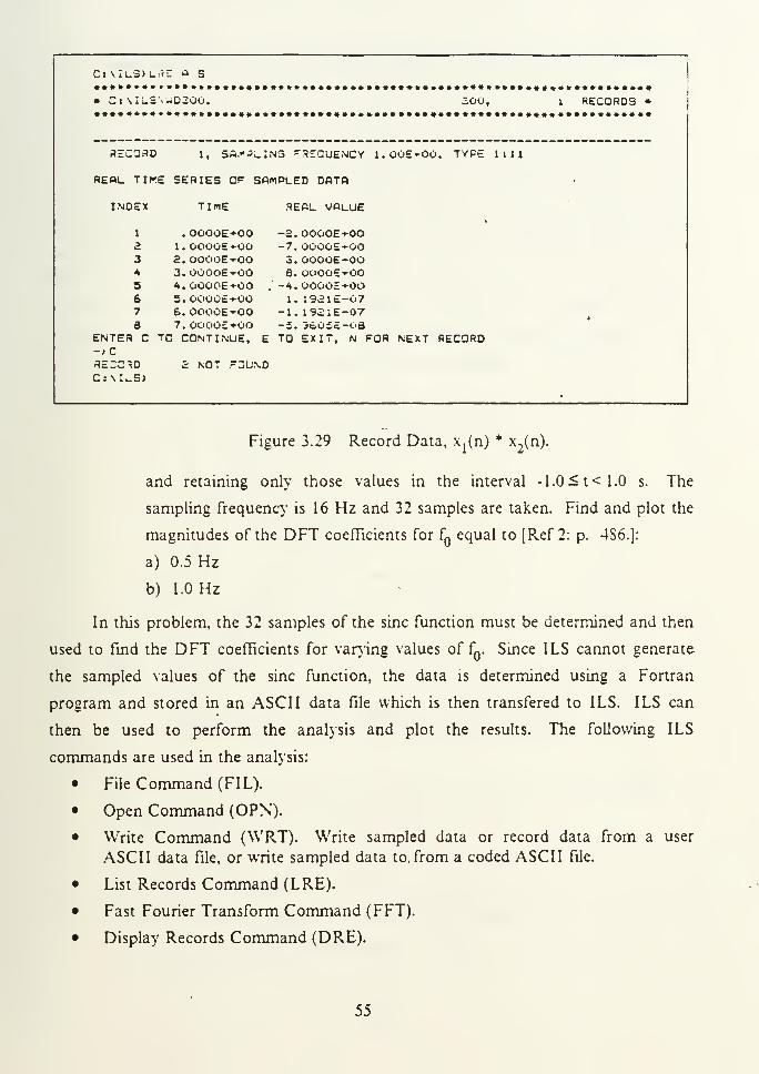
10. The results can be displayed numerically using LRE or graphically using
DRE. The file is secondary so the S argument must be used with either
command. The M and A arguments used with DRE display the magnitude of
the record while prompting for scaling options.
Input: LRE S
ILS responds with: Figure 3.29, a listing of the results of the convolution of
WD 200 and WD 20 1.
The result is displayed in figure 3.30 using DRE MAS. [Ref. 4]
Problem 6: Evaluate the DFT of the sequence found by sampling the analog signal:
2f sin(27if t)
fit)-
27tfQt
54
Cl\iL3>Lr) : a s
i
• Ci\IL='> ^D300. -OO, 1 RECORDS *
RECORD 1, sa*p;_;ng -recuency i.oos*oo, type miREAL TIKE SERIES OF SAMPLED DATP •
INDEX TIME REAL VALUE
1 . OOOOE+OO -a. ooooEt-oo3 1. OOOOE+OO -7. OOOOEt-OO3 2. OOOOE+OO 3. OOOOE*0O4 3. OOOOE+OO 8. OOOOE+OOS 4. OOOOE+OO -4. OOOOE+OO6 3. OOOOfct-OO 1. 1921E-077 6. OOOOE+OO -1. 1S21E-07a 7. OOOOE+OO -5. 36.05E-O8
ENTER C TC CONTINUE, E TO EXIT, N FOR NEXT RECORD->CRECCED 2 NOT FOUNDC:\I._S>
.
Figure 3.29 Record Data, Xj(n) * x2(n).
and retaining only those values in the interval -1.0^t<1.0 s. The
sampling frequency is 16 Hz and 32 samples are taken. Find and plot the
magnitudes of the DFT coefficients for fQequal to [Ref 2: p. 486.]:
a) 0.5 Hz
b) 1.0 Hz
In this problem, the 32 samples of the sine function must be determined and then
used to fmd the DFT coefficients for varying values of fQ
. Since ILS cannot generate
the sampled values of the sine function, the data is determined using a Fortran
program and stored in an ASCII data file which is then transfered to ILS. ILS can
then be used to perform the analysis and plot the results. The following ILS
commands are used in the analysis:
File Command (FIL).
Open Command (OPN).
Write Command (WRT). Write sampled data or record data from a user
ASCII data file, or write sampled data to, from a coded ASCII file.
List Records Command (LRE).
Fast Fourier Transform Command (FFT).
Display Records Command (DRE).
55

— ir»
— t**
- c-i
uj u i
<5»
in
ixi
•XIty»
lz A(Jt5*'ltO
Figure 3.30 Record Data, \.(n) * x,(n).
30
• Unary Operations Command (UOP). This command is used to perform unary
operations on signal processing record files.
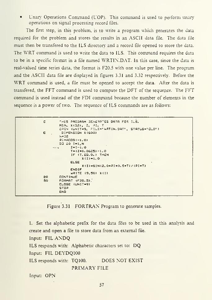
The first step, in this problem, is to write a program which generates the data
required for the problem and stores the results in an ASCII data 1"\1q. The data file
must then be transfered to the ILS directory and a record file opened to store the data.
The WRT command is used to write the data to ILS. This command requires the data
to be in a specific format in a file named WRTIN.DAT. In this case, since the data is
real-valued time series data, the format is F20.5 with one value per line. The program
and the ASCII data file are displayed in figures 3.31 and 3.32 respectively. Before the
WRT command is used, a file must be opened to accept the data. After the data is
transfered, the FFT command is used to compute the DFT of the sequence. The FFT
command is used instead of the FDI command because the number of elements in the
sequence is a power of two. The sequence of ILS commands are as follows:
c "HIS PRCGRAm 3E.v£^A~ES DATO FO^ ILS.REAl. X<32), 2, 31, T
CSiNi (UNIT-3, FILE"' WRTIN. DAT' , STATUS-' OLD' )
c DIMENSION X<600>;v»32PI-ACOS<-1.0>03 ftO I-l,N
-••-. Z-I-1.0T-<Z«0.06£5)-l.OIF <T. EQ.O. > THEN
X<I>-1.0ELSE
X < I > -SIN (a. 0»PI«0. 5»T)
/
<PI«T)ENDIFWRITE (9,30) X(I)
so CONTINUESO FORMAT (F20.S).'
CLOSE (UNIT-9)STOPEND
Figure 3.31 FORTRAN Program to generate samples.
1. Set the alphabetic prefix for the data files to be used in this analysis and
create and open a file to store data from an external file.
Input: FILANDQILS responds with: Alphabetic characters set to: DQInput: FILDEYDQ100
ILS responds with: TQ100. DOES NOT EXIST
PRIMARY FILE
Input: OPN
57

. 00000
.06624
. 13321
.2176S
. 3uO I 1
.38437
.47053
.55501
.£3662. 71359. 78431.84633. 90032.94317.97450. 99359
1 . OO0OO. 39359.97450.94317. 90032. 84633. 78421.71359. 63S62.55501.47053. 38*37. 300 1
1
.21765
. 13321
. 06624
Figure 3.32 Sampled Data from FORTRAN Program.
ILS responds with: (A system prompt.)
2. With the file DQ100 opened and ready to receive record data, the WRTcommand can be used to transfer data from the file WRTIN.DAT. The
alphabetic argument used by the WRT command is T, which tells ILS to store
real time series data from a file named WRTIN.DAT. The first numeric
argument of trie command identifies the number of items to store in each
record, the second identifies the number of elements in each record, the third
identifies the number of records to to use from WRTIN.DAT, and the fourth
and fifth are the integer multiple of the sampling frequency of the record and
the power of ten multiplier of the sampling frequency.
Input: WRTT32,1,32,16,0
ILS responds with: DQ100. RECORD 1 STORED
58
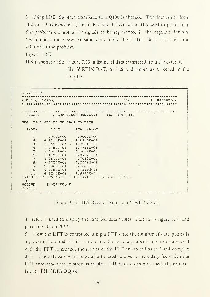
3. Using LRE, the data transferee! to DQ100 is checked. The data is not from
-1.0 to 1.0 as expected. (This is because the version of ILS used in performing
this problem did not allow signals to be represented in the negative domain.
Version 6.0, the newer version, does allow this.) This does not affect the
solution of the problem.
Input: LRE
ILS responds with: Figure 3.33, a listing of data transfered from the external
file, YYRTIN.DAT, to ILS and stored as a record in file
DQloO.
C: \;*_S: l_3E
* C:\IlS \2QiOO. 10'J, 1 RECG3D3 *
RECORD 1, SAMPLING FREQUENCY 16, TYPE 1111
REAl TI!*-£ SERIES OF SAMPLED DATA
INDEX TIME REA_ VALUEi
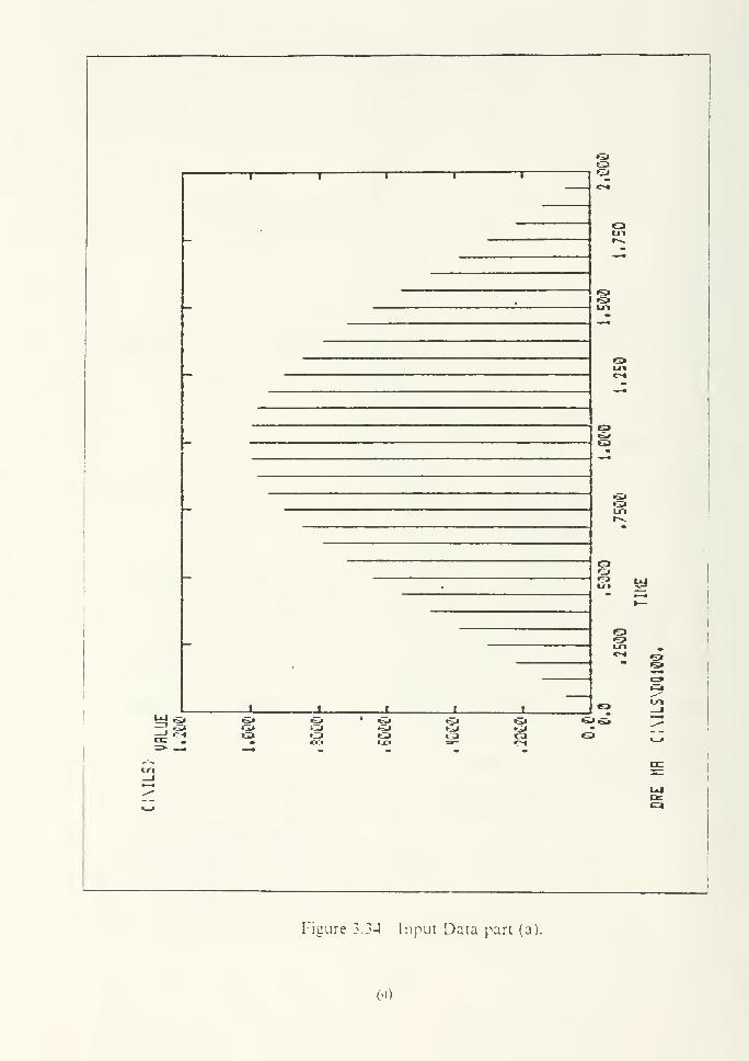
1 . OOOOE+OO . OOOOE+OO2 6. 2:500E-02: 6. EE40E-02:3 i. asooE-o: 1. 33E1E-014 1. 3750E-01 i. 176,32-013 E. 50OOE-OI 3. 001 IS-016 3. 1230E-01 3. 3437E-017 2. 7500E-01 4. 70521-0:a 4, 37502-01 5. 25012-013 5. OOOOE-Ol £.. 3EE2S-0;
10 5. e.2502-01 7. 13592-011
1
6. E3'X>E-01 7, a4£lE-0IE^TER C TO CONTINUE, E TO EXIT, N FGR NEXT REC3RD-I NSECOND E NOT FOUNDC: \I^3>
Figure 3.33 ILS Record Data from WRTIN.DAT.
4. DRL is used to display the sampled data values. Pari (a) is figure 3.34 and
part (b) is figure 3.35.
5. Now the DFT is computed using a FFT since the number of data points is
a power of two and this is record data. Since no alphabetic arguments are used
with the FFT command, the results of the FFT are stored as real and complex
data. The FIL commanJ must also be used to open a secondary file which the
FFT command uses to store its results. LRE is used again to check the results.
Input: FIL SDEYDQlOl
59
_L
fit
O
in
in
S3
G3
fZ)
o «
o«s»in<»! *TM
flf
1
^
J> J
•Li* jj ti»
Figure 5.34 Input Data part (a).
60
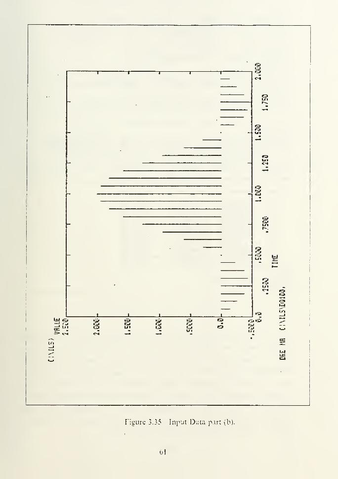
UJS, Si Si «^i i-^j^ *** Sj Si Si G>^ «-" S> in G> Si• U t
CI
SiS»«a»i
Ul
in
figure 3.35 Input Data part (b).
01

ILS responds with: DQ101. DOES NOT EXIST
SECONDARY FILE
Input: OPN S
ILS responds with: (A system prompt.)
Input: FFT ,,5
ILS responds with: DQ101. RECORD 1 STORED
Input: LRE S
ILS responds with: Figure 3.36, the DFT of the sine function.
Ci\ILS>LRE S
* Ci\ILS\DQ101. 101. 1 RECORDS »
•
(jernBTi t , CQMDI THJ6 CPEQUENCY 15, Tvpc 2211
COMPLEX RECTANGULAR SYMMETRIC SPECTRUM OF SAMPLED DATQ
INDEX FREQUENCY REA<_ VALUE i-lAG VALUE
1 . OOOOE+OO 1.8853E+01 .OOOOE+OO2 5. OOOOE-01 -7. 2331E+00 -9. l<*46£-08
3 l.OOOOE+OO -9. 1285E-01 -1.9717E-084 1.5000E+00 -3. 8754E-01 -7. 1470E-OS3 2. OOOOE+00 -2. 1834E-01 . 0OOO£*0O6 2. SOOOE+00 -1.4269E-01 -7. 4784E-087 3. OOOOE+OO -1.022*E-0l -2.6815E-08a 3. 5000E*00 -7.8153E-02 -4.8791E-089 4. OOOOE-K10 -6. 2800E-02 •OOOOE+OO10 4. 3000E«-00 -5. 2S05E-02 -2. 8721E-0711 5. 0OOOE«-OO -4. 5346E-02 -1. i9l*E-08
ENTER C TO CONTINUE, E TO EXIT, N FOR NEXT RECORD->NRECORD 2 NOT FOUNDCt\ILS>
Figure 3.36 DFT CoefTicients part (a).
6. The output file DQ101 contains the real and imaginary pans of the DFT but
not the magnitude. This file can be modified to contain the magnitude of the
DFT by using the UOP command. The LOP command does this by computing
the absolute value of the data in DQ101 and storing the results in a secondary
file. First the FIL command is used to change DQ101 to a primary file and
initialize a secondary file. The OPN command opens the secondary file to
accept the results of the UOP command. The UOP command uses the AB
argument to identify that it will compute the absolute value of the data in
DQ101. Default values for the numeric values are used.
62
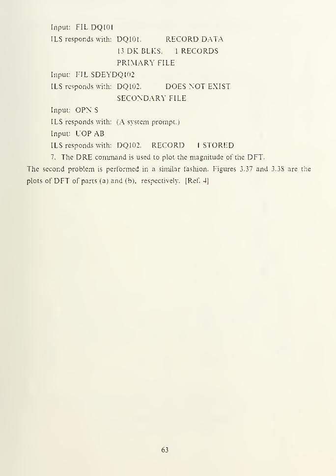
Input: FIL DQ101
I LS responds with: DQ101. RECORD DATA
13 DK BLKS, 1 RECORDS
PRIMARY FILE
Input: FIL SDEYDQ102
ILS responds with: DQ102. DOES NOT EXIST
SECONDARY FILE
Input: OPN S
ILS responds with: (A system prompt.)
Input: LOP AB
ILS responds with: DQ102. RECORD 1 STORED
7. The DRE command is used to plot the magnitude of the DFT.
The second problem is performed in a similar fashion. Figures 3.37 and 3.38 are the
plots of DFT of parts (a) and (b), respectively. [Ref. 4]
63
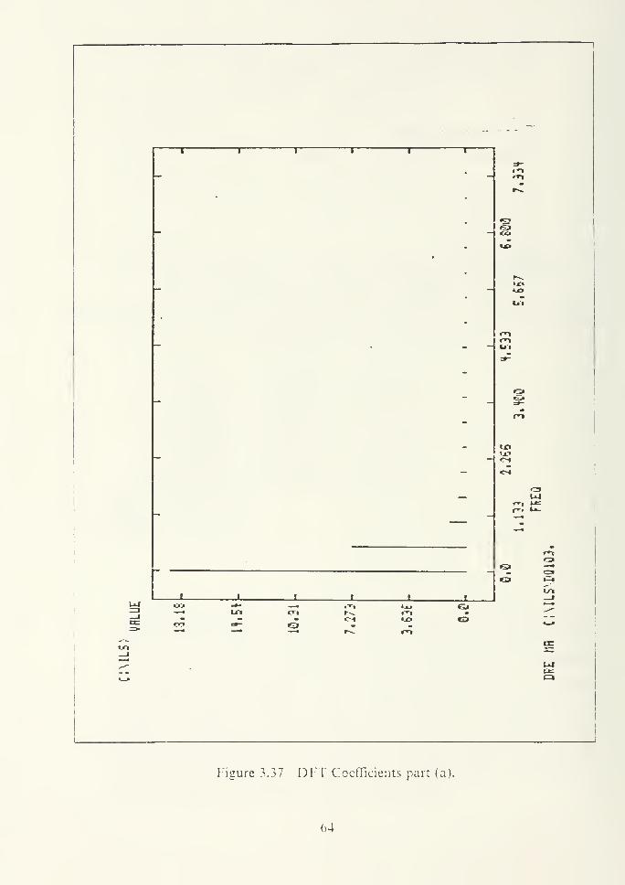
UJ•Tt •a» G»r^ m mc--i us Q
ut;
Figure 3.37 DFT Coefficients part (a).
04
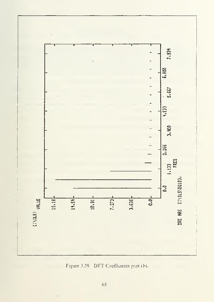
w o>
Figure 3.38 DFT Coefficients part (b)
65
IV. CONCLUSIONS
Having described the capabilities of ILS and worked several example problems,
an evaluation of the system is appropriate. The software package is evaluated in an
academic environment which consists of comparing the advantages and disadvantages
of ILS to existing digital signal processing tools at the Naval Postgraduate School.
A. DIGITAL SIGNAL PROCESSING TOOLS AT NPS
Presently, only the mainframe system has programs which perform digital signal
processing. These programs are available to the students by accessing a public disk.
The primary signal processing applications available through these programs are:
• Fast Fourier Transforms.
• Discrete Fourier Transforms.
• Frequency response of continuous and discrete systems.
• Convolution.
• Correlation.
• Difference equation solution.
The programs are not interactive and require creation of output files and reprograming
of subroutines within the programs in some cases. Plotting of the results from these
programs is obtained using DISSPLA or EASYPLOT.
The mainframe is compatible with a number of programing languages such as
FORTRAN, PASCAL, and APL. This allows the user to write signal processing
programs for applications which are not available through the public disk. One of the
more useful languages for application multidimensional signal processing analysis is
APL. APL is used primarily for solutions which require an iterative matrix type of
solution process. The results of an APL session are easily plotted using GRAFSTAT,
an interactive plotting, data analysis, and applied statistics software package which
uses APL.
B. ADVANTAGES AND DISADVANTAGES OF ILS
A comparison of PC-based ILS with existing mainframe signal processing tools
identifies the advantages and disadvantages of both systems. First, ILS has the
advantage of being readily accessible. There are no unscheduled or scheduled
66
maintenance requirements which affect the availability of ILS running on a personal
computer. ILS is completely interactive so no substantial programing ability is
required to use the software. The software can also be used in a menu driven
environment. This allows the user to obtain a better understanding of the ILS
commands and their usage in digital signal processing applications. The data generated
through the use of ILS commands and stored in ILS files is easily plotted with ILS
display commands. The ILS software can get data from external sources. The
software has the ability to convert and use data from an external data file and with
A D and DA boards, convert externally generated data to ILS format for processing
and then reconvert and output that data in its original format. This gives the user an
infinite variety of signals to generate and analyze.
There are some disadvantages with ILS, however. First ILS cannot perform
multidimensional signal processing. The software limits the number oC techniques
available for performing signal processing analysis. For example, the user cannot
design a recursive filter by other than the bilinear transform method. ILS does not
integrate with other programs or software. Thus, it is not possible to incorporate new
user-developed operations in the software. The graphics provided by the software does
not display well with dot matrix type printers and its plots are limited to the software
options and capabilities. For example, ILS will not smooth plots with curve fitting
options such as an cubic spline, it merely connects the points. Finally, the user must
have a very good understanding of digital signal processing techniques to apply the
software correctly and interpret ILS results.
C. RECOMMENDATION FOR EMPLOYMENTILS is a powerful signal processing tool. The software requires the user to have
a good foundation in signal processing techniques in order to use the system
effectively. The menu driven and interactive capability of ILS makes this version of
the software easier to use for beginners. Since the software consolidates a number of
signal processing methods, it would be utilized most efficiently as a research tool. ILS
could also perform as a lab tool for projects in courses which deal with spectral
analysis, digital filter design, and speech processing.
67
APPENDIX
ILS COMMAND: DFI
This appendix consists of an excerpt from the ILS Command Reference Guide.
It is representative of the documentation provided to the user concerning the
capabilities, usage and format of ILS commands.
68
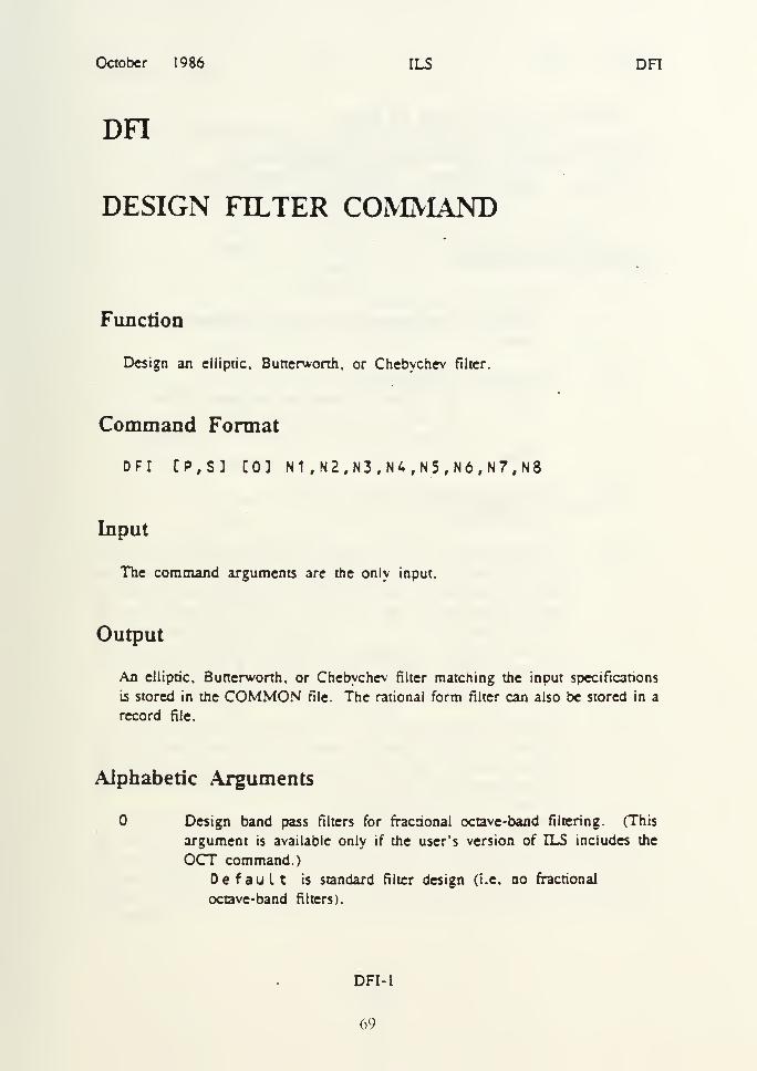
October 1986 ILS DFI
DH
DESIGN FILTER COMMAND
Function
Design an elliptic. Butter-worth, or Chebychev filter.
Command Format
DFI CP,S] CO] N1 ,N2, N3,N4,N5,N6,N7,N8
Input
The command arguments are the only input.
Output
An elliptic, Butterworth, or Chebychev filter matching the input specifications
is stored in the COMMON file. The rational form filter can also be stored in a
record file.
Alphabetic Arguments
Design band pass filters for fractional octave-band filtering. (This
argument is available only if the user's version of ILS includes the
OCT command.)
Default is standard filter design (i.e. no fractional
octave-band filters).
DFI-
1
69
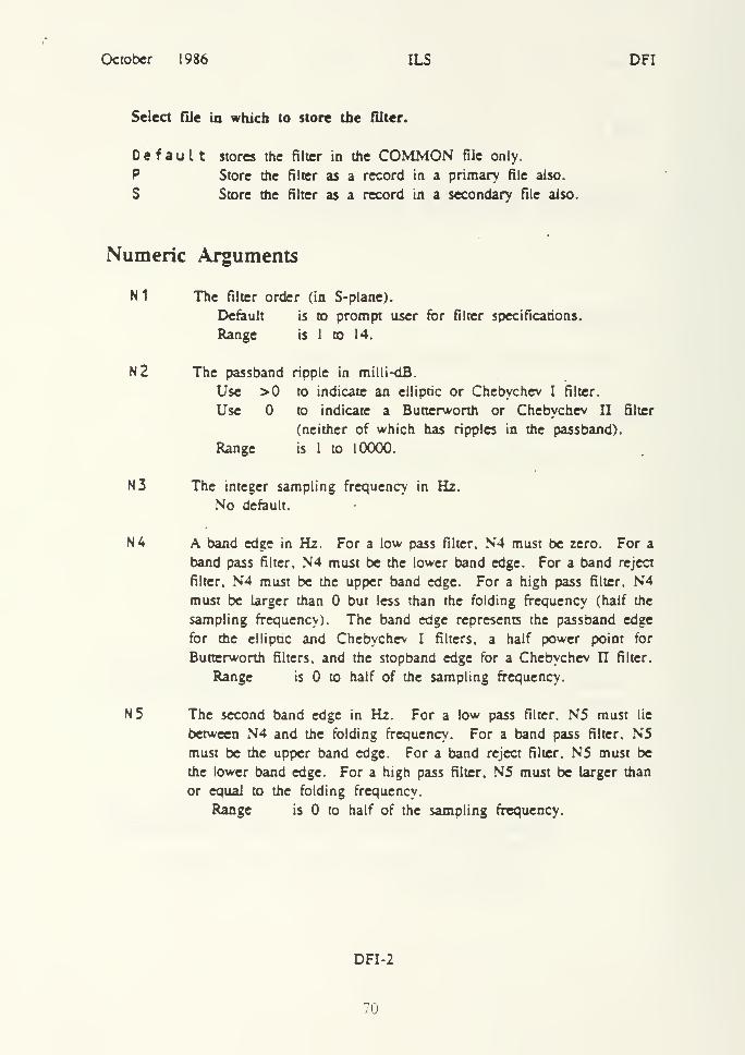
October 1986 ILS DFI
Select file in which to store the filter.
Default stores the filter in the COMMON file only.
P Store the Miter as a record in a primary file also.
S Store the filter as a record in a secondary file also.
Numeric Arguments
N
1
The filter order (in S-plane).
Default is to prompt user for filter specifications.
Range is 1 to 14.
N2 The passband ripple in milli-dB.
Use >0 to indicate an elliptic or Chebychev I filter.
Use to indicate a Butter-worth or Chebychev II filter
(neither of which has ripples in the passband).
Range is 1 to 10000.
N3 The integer sampling frequency in Hz.
No default.
N4 A band edge in Hz. For a low pass filter. N4 must be zero. For a
band pass filter, N4 must be the lower band edge. For a band reject
filter. N4 must be the upper band edge. For a high pass filter. N4must be larger than but less than the folding frequency (half the
sampling frequency). The band edge represents the passband edge
for the elliptic and Chebychev I filters, a half power point for
Butterworth filters, and the stopband edge for a Chebychev II filter.
Range is to half of the sampling frequency.
N5 The second band edge in Hz. For a low pass filter. N5 must lie
between N4 and the folding frequency. For a band pass filter. N5must be the upper band edge. For a band reject filter. N5 must be
the lower band edge. For a high pass filter. N5 must be larger than
or equal to the folding frequency.
Range is to half of the sampling frequency.
DFI-2
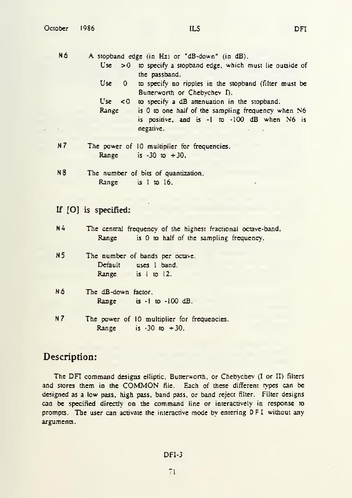
October 1986 ILS DFI
N6 A stopband edge (in Hz) or "dB-down" (in dB).
Use >0 to specify a stopband edge, which must lie outside of
the pass band.
Use to specify no ripples in the stopband (filter must be
Bunerworth or Chebychev I).
Use <0 to specify a dB attenuation in the stopband.
Range is to one half of the sampling frequency when N6is positive, and is -I to -100 dB when N6 is
negative.
N7 The power of 10 multiplier for frequencies.
Range is -30 to +30.
N3 The number of bits of quantization.
Range is I to 16.
If [O] is specified:
N4 The central frequency of the highest fractional octave-band.
Range is to half of the sampling frequency.
N5 The number of bands per octave.
Default uses 1 band.
Range is 1 to 12.
N6 The dB-down factor.
Range is -1 to -100 dB.
N 7 The power of 10 multiplier for frequencies.
Range is -30 to +30.
Description:
The DFI command designs elliptic. Bunerworth. or Chebychev (I or II) filters
and stores them in the COMMON file. Each of these different types can be
designed as a low pass, high pass, band pass, or band reject filter. Filter designs
can be specified directly on the command line or interactively in response to
prompts. The user can activate the interactive mode by entering DFI without any
arguments.
DFI-3
71
October 1986 ILS DFI
The spccmim of the filter can be displayed with the FDI C command (refer to
the example), and the filter can be used with commands such as FLT to filter
sampled data or record data. If specified by the user, the filter is stored in the
primary record file (P) or in the secondary record file (S) as well as in the
COMMON file.
The filters are designed as close to the user's specifications as possible. These
specifications include filter order, passband ripple, sampling frequency, passband
edges, stopband edge and required attenuation in stopband. The filter coefficient
design is printed at the end of the program (refer to the example). The numerator
and denominator coefficients and the corresponding quadratic factors (with the zero
order value of I suppressed) are stored in the COMMON file.
The printout consists of the following information:
1. Design specifications.
2. Denominator and numerator coefficients.
3. Poles and zeros (real and imaginary parts).
4. Quadratic factors for each pole or zero. Each complex pole or zero pair of the
form [1 - (a+jb)z**-l], [1 - (a-jb)z**-l], where a and b are complex
conjugate pole pairs, can be written as 1 - (2a)z**-l + (a**2 + b**2)z**-2.
The first order quadratic factor is (-2a) and the second order quadratic factor
is (a**2 + b**2).
5. Time constant. The time constant is the number of samples for the impulse
response of the pole closest to the unit circle to decay to 0.37 (1/e) of its
initial value. In general, if the value exceeds 100. the filter may be
ill-designed.
6. Noise bandwidth. The noise bandwidth is the theorencai equivalent bandwidth
for white noise input. It is the value for which an ideal filter (gain of one in
passband. zero otherwise) would produce the same energy.
If the filter order (N1) is not entered, the program prompts for the parameter
values. The order of the filter is usually specified as less than 10 since higher
order filters can produce numeric instabilities. An order of 3 or 4 is typical.
DFI-4
72
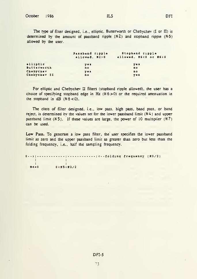
October 1986 ILS DFI
The rype of filler designed, i.e.. elliptic. Butterworth or Chebychev (I or II) is
determined by the amount of passband ripple (N2) and stopband ripple (N6)
allowed by the user
ftiib*od cippl* Stopband rippl*illawtd, S2>0 allowed, B6<0 or »6>0
• lliptie y • • y •
•
tutttcworth do ooCh«bycb«v y«g noCb«byeb«v II no y»*
For elliptic and Chebychev n filters (stopband ripple allowed), the user has a
choice of specifying stopband edge in Hz (N6>0) or the required attenuation in
the stopband in dB (N6<0).
The class of filter designed, i.e.. low pass, high pass, band pass, or band
reject, is determined by the values set for the lower passband limit (N4) and upper
passband limit (N5). If these values are large, the power of 10 multiplier (N7)
can be used.
Low Pass. To generate a low pass filter, the user specifies the lower passband
limit as zero and the upper passband limit as greater than zero but less than the
folding frequency, i.e.. half the sampling frequency.
0-->|i |<--£oldinq fr*qu«oey (H3/2)
I I
I I
S4-C 0<5S<S3/2
DFI-5
15
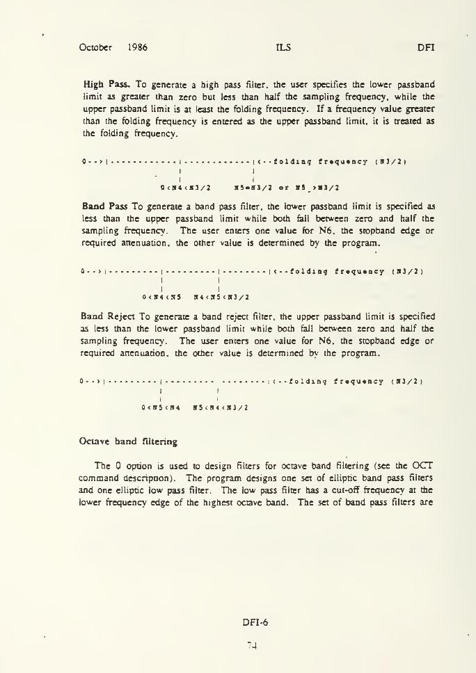
October 1986 ILS DFI
High Pass. To generate a high pass filter, the user specifies the lower passband
limit as greater than zero but less than half the sampling frequency, while the
upper passband limit is at least the folding frequency. If a frequency value greater
than the folding frequency is entered as the upper passband limit, it is treated as
the folding frequency.
0-->i | i<--fol4in<j (rtquincy (S3/2)I I
I I
0<S4<B3/2 SS-SJ/2 or SS >B3/2
Band Pass To generate a band pass filter, the lower passband limit is specified as
less than the upper passband limit while both fail between zero and half the
sampling frequency. The user enters one value for N6. the stopband edge or
required attenuation, the other value is determined by the program.
0-->i | | |<•- folding froquoncy (B3/2)
0<H4 <N5 S4<B5 <S3/2
Band Reject To generate a band reject filter, the upper passband limit is specified
as less than the lower passband limit while both fall between zero and half the
sampling frequency. The user enters one value for N6. the stopband edge or
required attenuation, the other value is determined by the program.
>I I-- <
i(•folding froquoncy ( S3/2
)
I I
Ii
<H5 <B4 ET S < It 4 <B3/2
Octave band filtering
The option is used to design filters for octave band filtering (see the OCTcommand description). The program designs one set of elliptic band pass filters
and one elliptic low pass filter. The low pass filter has a cut-off frequency at the
lower frequency edge of the highest octave band. The set of band pass filters are
DFI-6
74
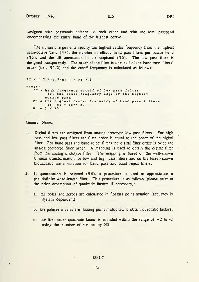
October 1986 ILS DFI
designed with passbands adjacent to each other and with the total passband
encompassing the entire band of the highest octave.
The numeric arguments specify the highest center frequency from the highest
semi-octave band (N4), the number of elliptic band pass filters per octave band
(N5). and the dfi attenuation in the stopband (N6). The low pass filter is
designed transparently. The order of the filter is one half of the band pass filters'
order (i.e.. N1/2) and the cutoff frequency is calculated as follows:
FC - [ 2 •• ( . 5«H) J• TH * .
3
whir* :
FC high frequency cutoff of low pass filter(or, the lower frequency edge of the highestoctave bend)the highest center frequency of bend pess filters(or, N4 • 10** H7)1 / H5
ra
General Notes:
I. Digital filters are designed from analog prototype low pass filters. For high
pass and low pass filters the filter order is equal to the order of the digital
filter. For band pass and band reject filters the digital filter order is twice the
analog prototype filter order. A mapping is used to obtain the digital filter-
frora the analog prototype filter. The mapping is based on the well-known
bilinear transformanon for low and high pass filters and on the lesser-known
biquadratic transformation for band pass and band reject filters.
2. If quantization is selected (NS). a procedure is used to approximate a
pseudofinite word-length filter. This procedure is as follows (please refer to
the prior description of quadratic factors if necessary):
a. the poles and zeroes are calculated in floating point notation (accuracy is
system dependent);
b. the pole/zero pairs are floating point multiplied to obtain quadratic factors;
c. the first order quadratic factor is rounded within the range of +2 to -2
using the number of bits set by N8;
DFI-7
o
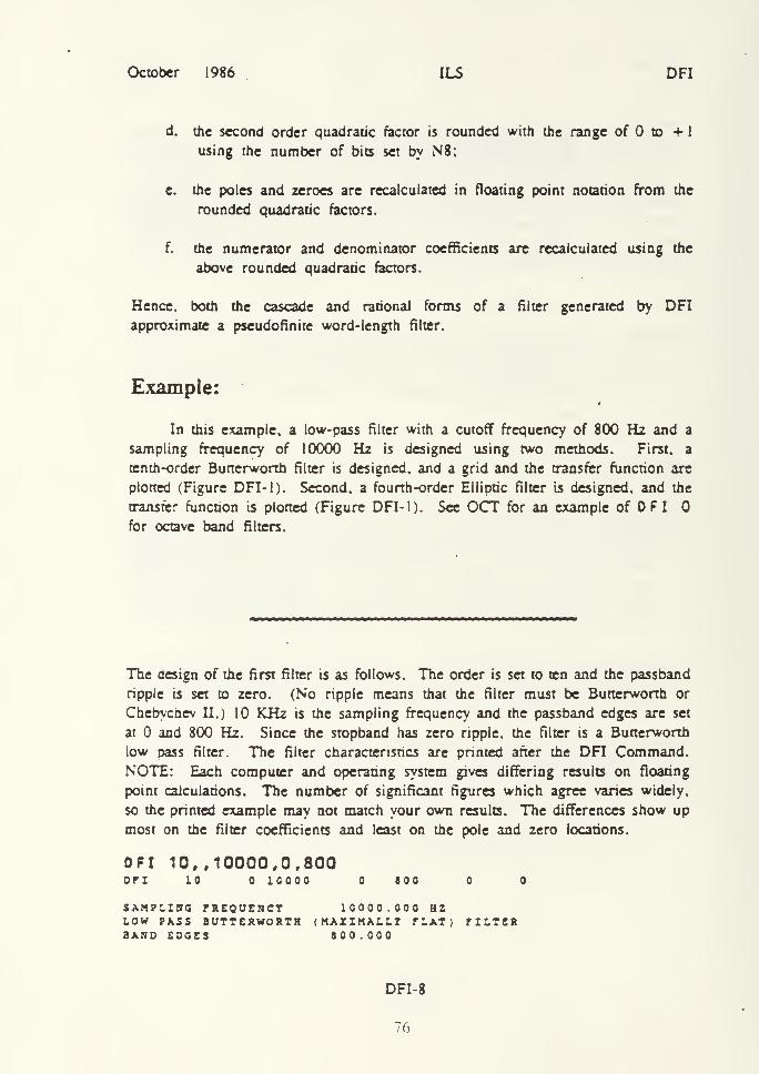
October 1986 ILS DFI
d. the second order quadratic factor is rounded with the range of to +1using the number of bits set by N8;
e. the poles and zeroes are recalculated in floating point notation from the
rounded quadratic factors.
f. the numerator and denominator coefficients are recalculated using the
above rounded quadratic factors.
Hence, both the cascade and rational forms of a filter generated by DFIapproximate a pseudofinite word-length filter.
Example:
In this example, a low-pass filter with a cutoff frequency of 800 Hz and a
sampling frequency of 10000 Hz is designed using two methods. First, a
tenth-order Butterworth filter is designed, and a grid and the transfer function are
plotted (Figure DFI- 1). Second, a fourth-order Elliptic filter is designed, and the
transfer function is plotted (Figure DFI-1). See OCT for an example of D F I
for octave band filters.
The design of the first filter is as follows. The order is set to ten and the passband
ripple is set to zero. (No ripple means that the filter must be Butterworth or
Chebychev II.) 10 KHz is the sampling frequency and the passband edges are set
at and 800 Hz. Since the stopband has zero ripple, the filter is a Butterworth
low pass filter. The filter characteristics are printed after the DFI Command.NOTE: Each computer and operating system gives differing results on floating
point calculations. The number of significant figures which agree varies widely,
so the printed example may not match your own results. The differences show up
most on the filter coefficients and least on the pole and zero locations.
DFI 10, ,10000,0,800op: io o ioooo o soo o o
SAMPLING FREQUENCY 10000.000 HZLOW PASS BUTTERWORTH (MAXIMALLT TLAT) FILTERBAND EDGES 300.000
DFI-8
76
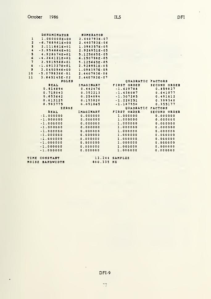
October 1986 ILS DFI
DENOMINATOR NUMERATOR1 . 0OOOO0E + 00 2 . 440793E • 07
• 6 . 738961E+G0 2
.
440793E 062 . 1 1186 1E + 01 1 . 098357E 05
•3
.
934664E+01 2.928951E •OS4
.
928074E+01 5.12S665E -05•4
.
264121E+01 6 .1S079SE 052 . 59 15 58E-01 5 . 12S66SE OS
•1.0 9 13 37E>01 2 .928931E- OS3
.
045054E+00 1
.
0983S7E 0510 - 5 . 798 36E- 01 2
.
440793E- 0611 3.84S145E-02 2
.
440793E- 07POLES QUADRATIC FACTORS
REAL IMAGINARY riRST ORDER SECOND ORDER. 814894 0.442476 • 1
.
629788 0.859837. 719043 0.352213 •1.438087 0.641077. 633642 0.254094 •1.307285 0.491812. 613125 . 153026 -1 . 226251 0.399340. 593775 . 051065 -1 . 187550 0.355177
ZEROS QUADRATIC FACTORSREAL IMAGINARY riRST ORDER SECOND ORDER
• 1 . 000000 0.000000 1 . 000000 0.000000•1.000000 . 000000 1.000000 0.000000•1
.
000000 . 000000 1.000000 0.000000•1.000000 .000000 1.000000 0.000000•1.000000 . 000000 1.000000 0.000000•1.000000 . 000000 1.000000 0.000000•1.000000 0.000000 1.000000 0.000000•1.000000 0.000000 1
.
000000 0.000000•1.000000 0.000000 1
.
000000 0.000000•1 . 000000 . 000000 1.000000 0.000000
TIME CONSTANT 13 . 244 SAMPLZSNOISE BANDWIDTH 800 . 335 HZ
DFI-9

October 1986 ILS DFI
FDI CE is used to display the filter response from the parameters stored in the
COMMON file and erase the screen before the display (E) (Figure DFI-1).
FDI CE
A grid is placed with a border and a vertical dotted line at the 800 Hz point.
GRO B,,800
DFI is used to design the second filter as a fourth-order filter, with a 200 mdBripple in the passband (so that the filter must be either elliptic or Chebychev I),
and a sampling frequency of 10 kHz. Since the band edges are entered in reverse
order. N5 is less than N4. the filter is a stopband filter, with passband edges of
3000 Hz and 2000 Hz. N6--50 specifies 50 dB attenuation in the stopband. so
that the filter must be of a type with ripples in the stopband. making it an elliptic
filter.
DPI 4,200,10000,3000,2000.-50DTI 4 200 10000 3000 2000 -SO
BIfD RJCT ELLIPTIC riLTERPASS BAND RIPPLE 0.200 OBPASS BARD EDGES 2000.000 3000.000 HZSTOP BARD EDGES 2276.582 2723.419 HZSAMPLING FREQUENCY 10000.000 HZATTEHUATIOS -50.000 OB
DENOMINATOR NUMERATOR1 . 000O0OE+O0 4.489288E-012.384186E-07 1.605494E-072 . 39 2886E+00 1.759466E+004.023314E-07 4.716140E-072 . 429392E+00 2 . 6 2 1 4 6 4 E +
2.980232E-07 4.749588E-071 .146745E+00 1.759466E+00
DFI- 10
7S
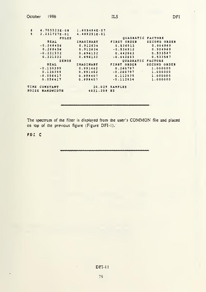
October 1986 ILS DFI
8 6 .705523E-08 1 .60S494E- 079 2.331727E-01 4 . 489291E- 01
POLES QUADRATIC fACTORSREAL IMAGINARY riRST ORDER SECOND ORDER
• . 268456 . 912634 . 536913 0.904969. 268456 0.912634 •0.536912 0.904969
•0.2213 32 .696132 . 442663 0.5335870.221332 0.696132 • . 442663 0.533587
ZEROS QUADRATIC FACTORSREAL IMAGINARY PIRST ORDER SECOND ORDER
-0 .130399 . 991462 . 260797 1 . 0000000.130399 0.991462 -0 .260797 1.000000
•0 .056417 0.998407 . 112835 1.000000.056417 0.998407 •0.112834 1 .000000
TIME CONSTANT 20.029 SAMPLESNOISE BANDWIDTH 4021.208 HZ
The spectrum of the filter is displayed from the user's COMMON file and placed
od top of the previous figure (Figure DFI- 1).
FDI C
DFI-tl
79
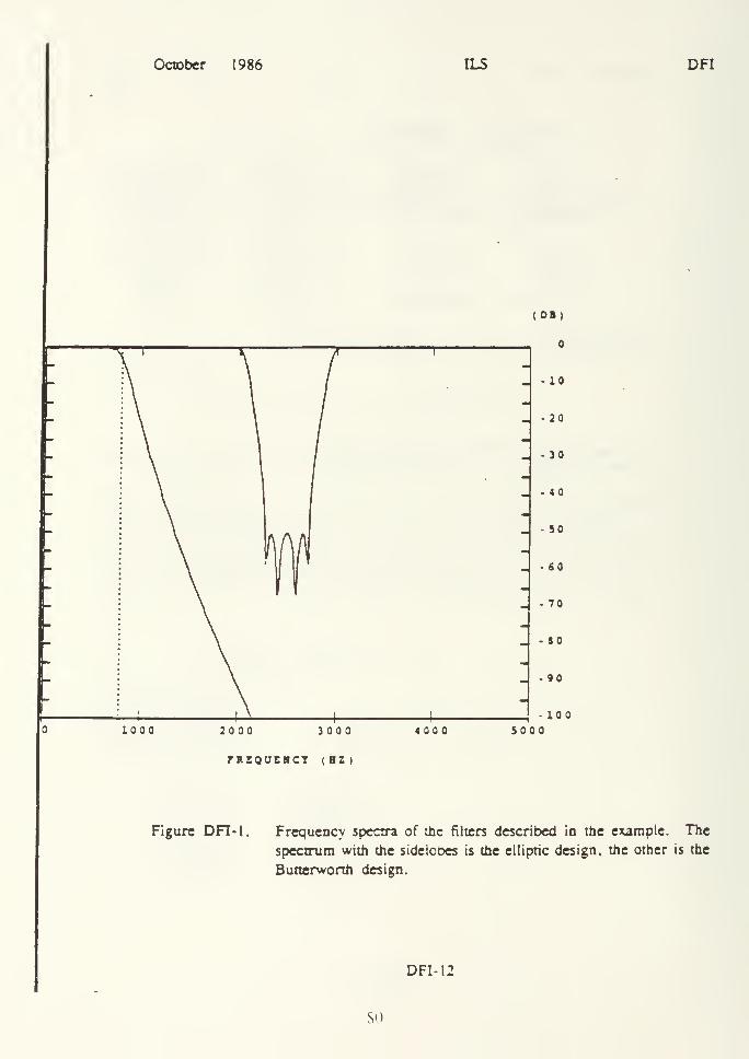
October 1986 ILS DFI
2000 3000
fRBQUEBCT (HZ)
Figure DFT-l. Frequency spectra of the filters described in the example. The
spectrum with the sidelobes is the elliptic design, the other is the
Butterworth design.
DFI- 12
SO
LIST OF REFERENCES
1. Information in a letter to Professor Donald E. Kirk from Professor Charles W.
Thernen Naval Postgraduate School. Monterey, CA dated 14 January 1987.
2. ILS User's Guide V6.0 PC DOS, Signal Technology Inc., Goleta, CA, 1987,
3. Strum, R. D. and Kirk, D. E., First Principles of Discrete Systems and Digital
Signal Processing Addison-Wesley Publishing Company, Inc., Menlo Park, CA,1988.
4. ILS Command Reference Guide, Signal Technology Inc., Goleta, CA, 19S7.
81
BIBLIOGRAPHY
Rabiner, Lawrence R., and Gold, Bernard, Theory and Application of Digital Signal
Processing, Prentice-Hall, Inc.. 1975.
82
INITIAL DISTRIBUTION LIST
No. Copies
1. Defense Technical Information Center 2
Cameron Station
Alexandria, VA 22304-6145
2. Library, Code 0142 2
Naval Postgraduate School
Monterey, CA 93943-5002
3. Chairman. Code 62 1
Director of Electrical and Computer Engineering
Naval Postgraduate School
Monterey. CA 93943-5000
4. Professor Roberto Cristi, Code 62Cx 1
Naval Postgraduate School
Monterey, CA 93943-5000
5. Lt. Janine England, Code 62Eg 1
Naval Postgraduate School
Monterey, CA 93943-5000
6. Professor Ralph Hippenstiel, Code 62Hi 1
Naval Postgraduate School
Monterey, CA 93943-5000
7. Professor Donald E. Kirk, Code 62Ki 1
Naval Postgraduate School
Monterey, CA 93943-5000
8. Professor Chin-Hwa Lee, Code 62Le 1
Naval Postgraduate School
Monterey, CA 93943-5000
9. Professor Paul H. Moose, Code 62Me 1
Naval Postgraduate School
Monterey, CA 93943-5000
83
10. Captain Thomas A. Quintero, L'SMCMarine Corps Tactical Systems Support Activity
Camp Pendelton, CA 92055-5080
1 1. Professor Robert D. Strum, Code 62St
Naval Postgraduate School
Monterey, CA 93943-5000
12. Professor Charles Therrien. Code 62Ti
Naval Postgraduate School
Monterey, CA 93943-5000
84


ThesisQ721c.l
QuinteroAn evaluation of Inter-
active Laboratory SystemSoftware, ILS-PC/DOS, adigital signal processingsoftware package.
Thesis
Q721
c.l
Quintero
fi^ evaluation of Inter-
active Laboratory System
Software, ILS-PC/DOS, a
digital signal processing
software package.

Recommended