Three things everyone should knowto improve object retrieval
University of Oxford 2nd April 2012
Relja Arandjelović and Andrew Zisserman (CVPR 2012)
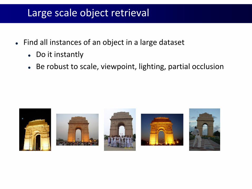
Large scale object retrieval
Find all instances of an object in a large dataset
Do it instantly
Be robust to scale, viewpoint, lighting, partial occlusion
Three things everyone should know
1. RootSIFT
2. Discriminative query expansion
3. Database-side feature augmentation

[Lowe04, Philbin07][Chum07]
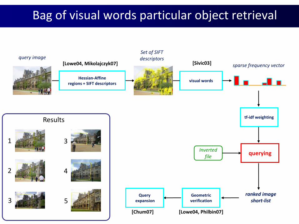
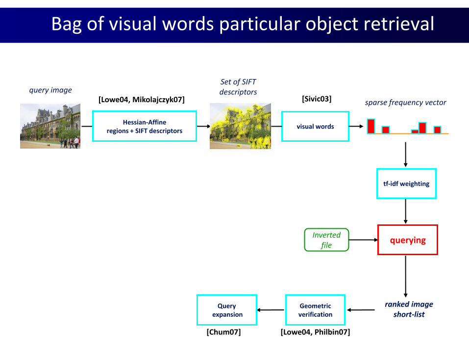
Hessian-Affineregions + SIFT descriptors
visual words
querying
sparse frequency vector
Invertedfile
ranked imageshort-list
Set of SIFTdescriptorsquery image
Geometricverification
Queryexpansion
[Lowe04, Mikolajczyk07] [Sivic03]
tf-idf weighting
Bag of visual words particular object retrieval
[Lowe04, Philbin07][Chum07]
Hessian-Affineregions + SIFT descriptors
visual words
querying
sparse frequency vector
Invertedfile
ranked imageshort-list
Set of SIFTdescriptorsquery image
Geometricverification
Queryexpansion
[Lowe04, Mikolajczyk07] [Sivic03]
tf-idf weighting
Bag of visual words particular object retrieval
1
2
3
3
4
5
Results
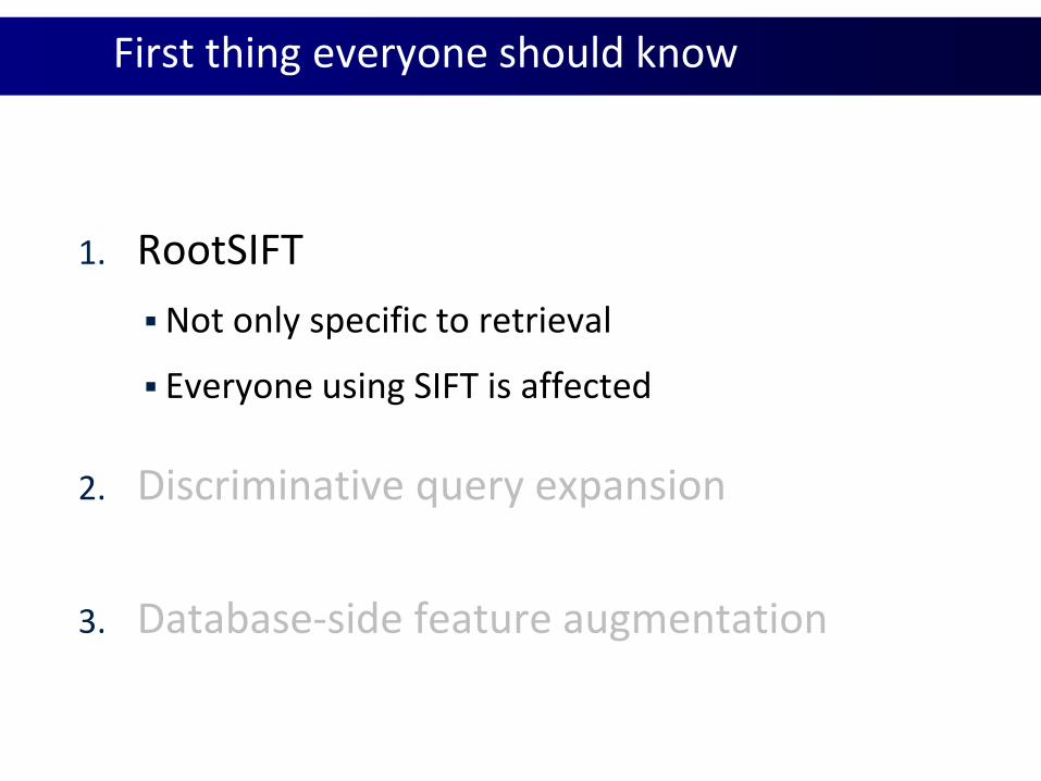
First thing everyone should know
1. RootSIFT
Not only specific to retrieval
Everyone using SIFT is affected
2. Discriminative query expansion
3. Database-side feature augmentation
Improving SIFT
Hellinger or χ2 measures outperform Euclidean distance
when comparing histograms, examples in image
categorization, object and texture classification etc.
These can be implemented efficiently using approximate
feature maps in the case of additive kernels
SIFT is a histogram: can performance be boosted using a
better distance measure?
Yes!
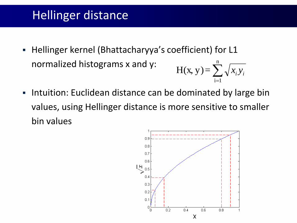
Hellinger distance
Hellinger kernel (Bhattacharyya’s coefficient) for L1
normalized histograms x and y:
Intuition: Euclidean distance can be dominated by large bin
values, using Hellinger distance is more sensitive to smaller
bin values
n
1i
=y)H(x, ii yx
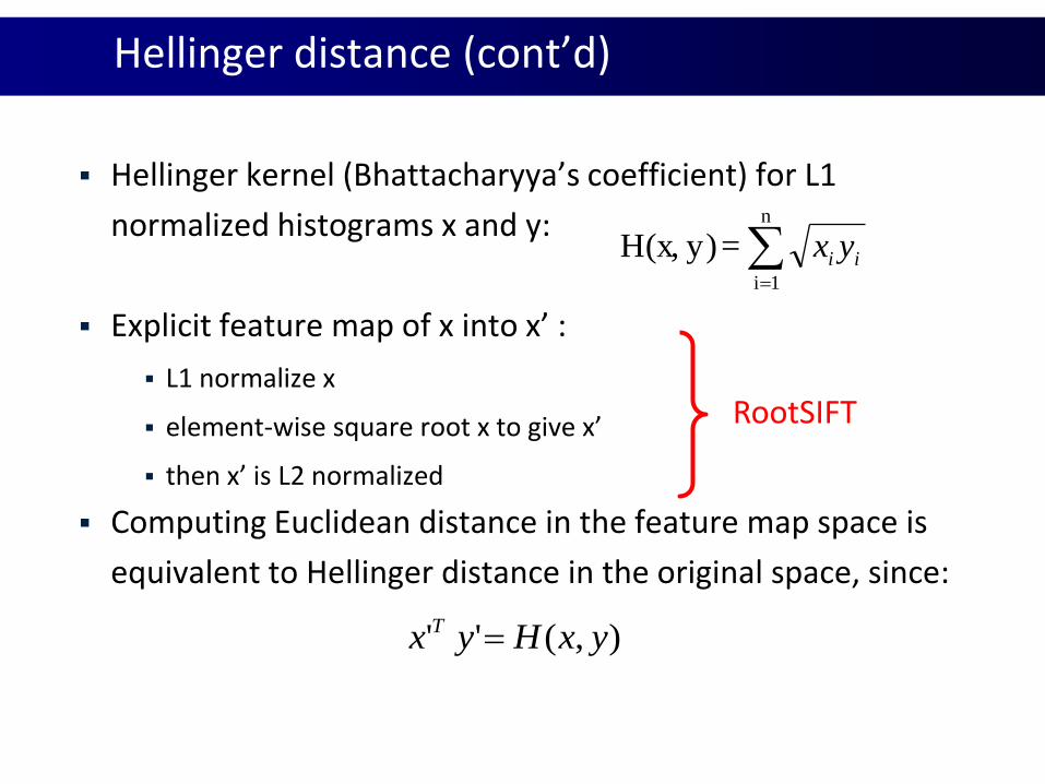
Hellinger distance (cont’d)
Hellinger kernel (Bhattacharyya’s coefficient) for L1
normalized histograms x and y:
Explicit feature map of x into x’ :
L1 normalize x
element-wise square root x to give x’
then x’ is L2 normalized
Computing Euclidean distance in the feature map space is
equivalent to Hellinger distance in the original space, since:
n
1i
=y)H(x, ii yx
),('' yxHyx T
RootSIFT
[Lowe04, Philbin07][Chum07]
Hessian-Affineregions + SIFT descriptors
visual words
querying
sparse frequency vector
Invertedfile
ranked imageshort-list
Set of SIFTdescriptorsquery image
Geometricverification
Queryexpansion
[Lowe04, Mikolajczyk07] [Sivic03]
tf-idf weighting
Bag of visual words particular object retrieval
[Lowe04, Philbin07][Chum07]
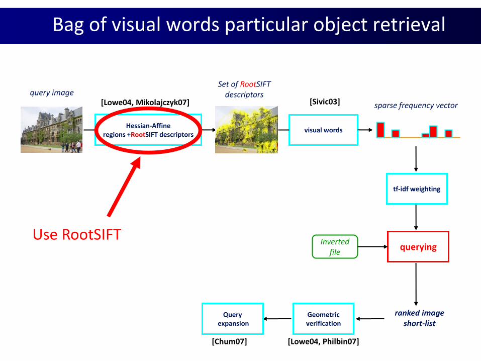
Hessian-Affineregions +RootSIFT descriptors
visual words
querying
sparse frequency vector
Invertedfile
ranked imageshort-list
Set of RootSIFTdescriptorsquery image
Geometricverification
Queryexpansion
[Lowe04, Mikolajczyk07] [Sivic03]
tf-idf weighting
Use RootSIFT
Bag of visual words particular object retrieval
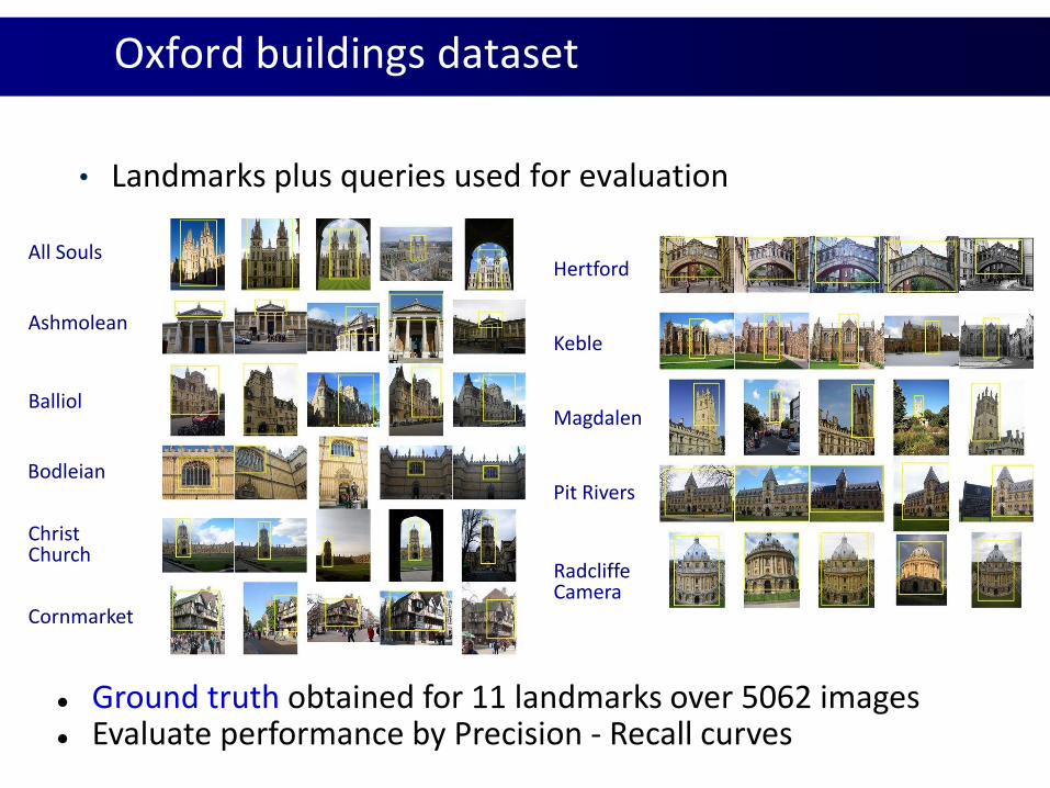
Oxford buildings dataset
• Landmarks plus queries used for evaluation
All Souls
Ashmolean
Balliol
Bodleian
Christ Church
Cornmarket
Hertford
Keble
Magdalen
Pit Rivers
Radcliffe Camera
Ground truth obtained for 11 landmarks over 5062 images Evaluate performance by Precision - Recall curves
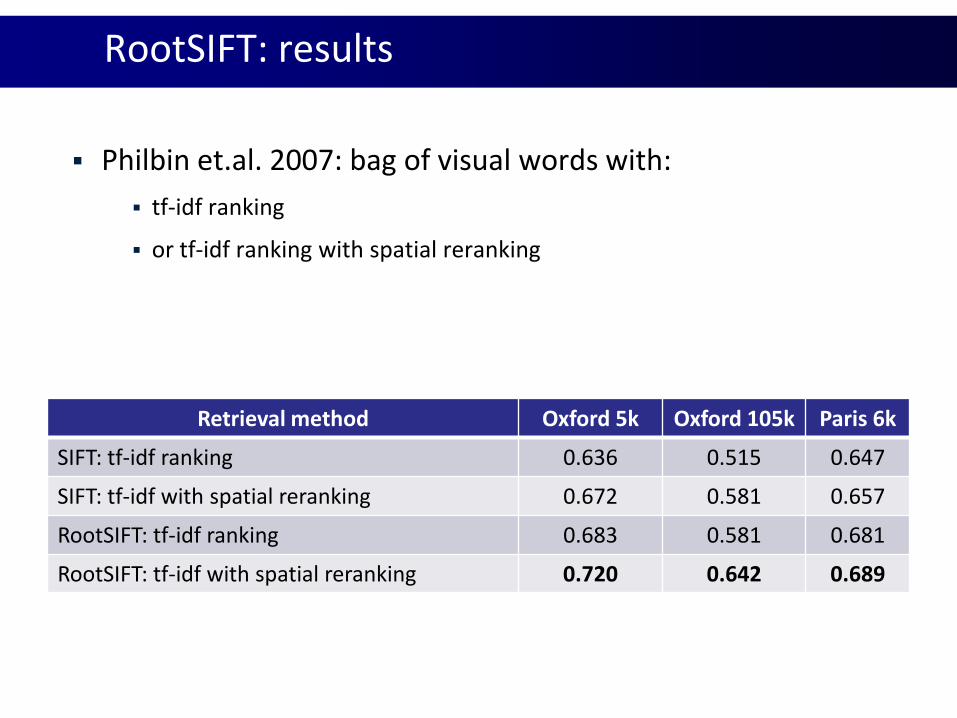
RootSIFT: results
Philbin et.al. 2007: bag of visual words with:
tf-idf ranking
or tf-idf ranking with spatial reranking
Retrieval method Oxford 5k Oxford 105k Paris 6k
SIFT: tf-idf ranking 0.636 0.515 0.647
SIFT: tf-idf with spatial reranking 0.672 0.581 0.657
RootSIFT: tf-idf ranking 0.683 0.581 0.681
RootSIFT: tf-idf with spatial reranking 0.720 0.642 0.689
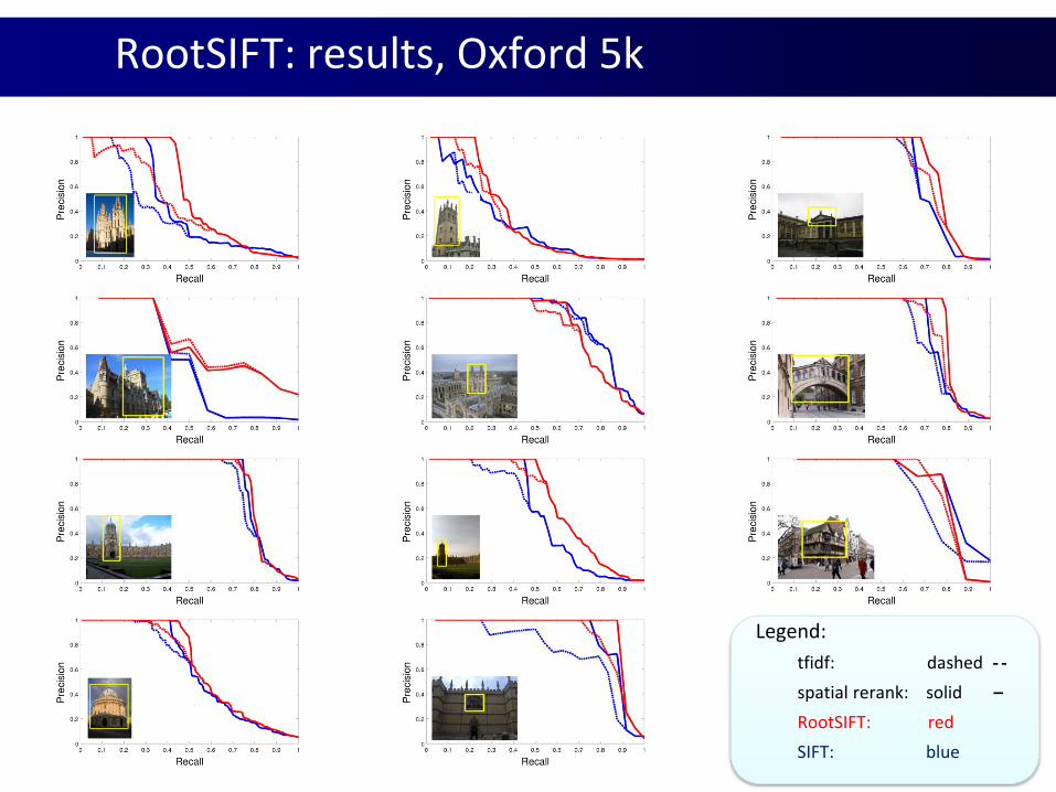
RootSIFT: results, Oxford 5k
Legend:
tfidf: dashed - -
spatial rerank: solid –
RootSIFT: red
SIFT: blue
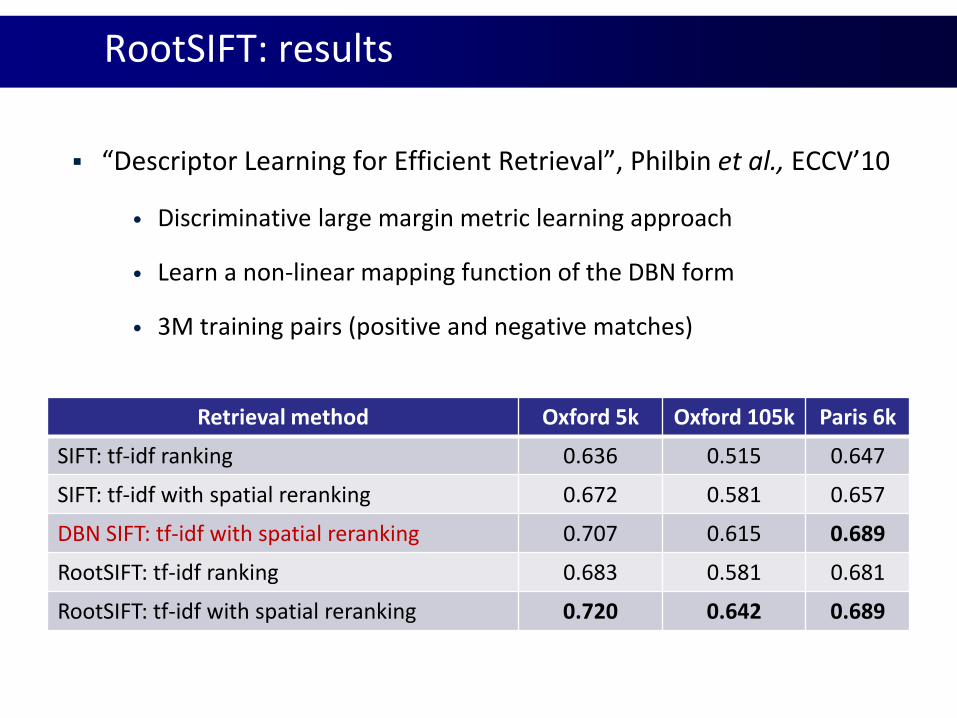
RootSIFT: results
“Descriptor Learning for Efficient Retrieval”, Philbin et al., ECCV’10
• Discriminative large margin metric learning approach
• Learn a non-linear mapping function of the DBN form
• 3M training pairs (positive and negative matches)
Retrieval method Oxford 5k Oxford 105k Paris 6k
SIFT: tf-idf ranking 0.636 0.515 0.647
SIFT: tf-idf with spatial reranking 0.672 0.581 0.657
DBN SIFT: tf-idf with spatial reranking 0.707 0.615 0.689
RootSIFT: tf-idf ranking 0.683 0.581 0.681
RootSIFT: tf-idf with spatial reranking 0.720 0.642 0.689
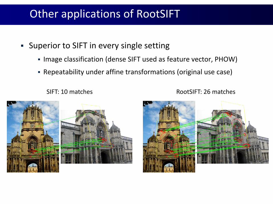
Other applications of RootSIFT
Superior to SIFT in every single setting
Image classification (dense SIFT used as feature vector, PHOW)
Repeatability under affine transformations (original use case)
SIFT: 10 matches RootSIFT: 26 matches
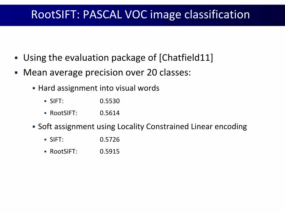
RootSIFT: PASCAL VOC image classification
Using the evaluation package of [Chatfield11]
Mean average precision over 20 classes:
Hard assignment into visual words
SIFT: 0.5530
RootSIFT: 0.5614
Soft assignment using Locality Constrained Linear encoding
SIFT: 0.5726
RootSIFT: 0.5915
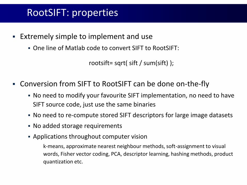
RootSIFT: properties
Extremely simple to implement and use
One line of Matlab code to convert SIFT to RootSIFT:
rootsift= sqrt( sift / sum(sift) );
Conversion from SIFT to RootSIFT can be done on-the-fly
No need to modify your favourite SIFT implementation, no need to have
SIFT source code, just use the same binaries
No need to re-compute stored SIFT descriptors for large image datasets
No added storage requirements
Applications throughout computer vision
k-means, approximate nearest neighbour methods, soft-assignment to visual
words, Fisher vector coding, PCA, descriptor learning, hashing methods, product
quantization etc.
RootSIFT: conclusions
Superior to SIFT in every single setting
Every system which uses SIFT is ready to use RootSIFT
No added computational or storage costs
Extremely simple to implement and use
We strongly encourage everyone to try it!
Second thing everyone should know
1. RootSIFT
2. Discriminative query expansion
3. Database-side feature augmentation
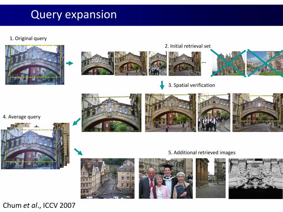
1. Original query
3. Spatial verification
4. Average query
…
2. Initial retrieval set
5. Additional retrieved images
Chum et al., ICCV 2007
Query expansion
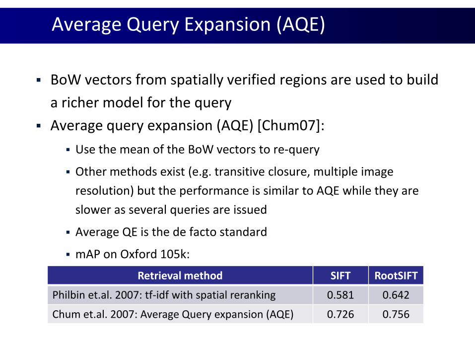
Average Query Expansion (AQE)
BoW vectors from spatially verified regions are used to build
a richer model for the query
Average query expansion (AQE) [Chum07]:
Use the mean of the BoW vectors to re-query
Other methods exist (e.g. transitive closure, multiple image
resolution) but the performance is similar to AQE while they are
slower as several queries are issued
Average QE is the de facto standard
mAP on Oxford 105k:
Retrieval method SIFT RootSIFT
Philbin et.al. 2007: tf-idf with spatial reranking 0.581 0.642
Chum et.al. 2007: Average Query expansion (AQE) 0.726 0.756
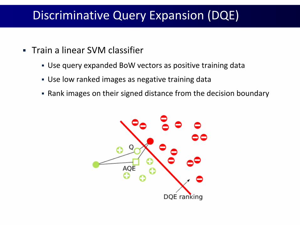
Discriminative Query Expansion (DQE)
Train a linear SVM classifier
Use query expanded BoW vectors as positive training data
Use low ranked images as negative training data
Rank images on their signed distance from the decision boundary
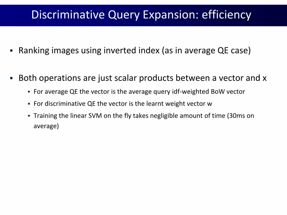
Discriminative Query Expansion: efficiency
Ranking images using inverted index (as in average QE case)
Both operations are just scalar products between a vector and x
For average QE the vector is the average query idf-weighted BoW vector
For discriminative QE the vector is the learnt weight vector w
Training the linear SVM on the fly takes negligible amount of time (30ms on
average)
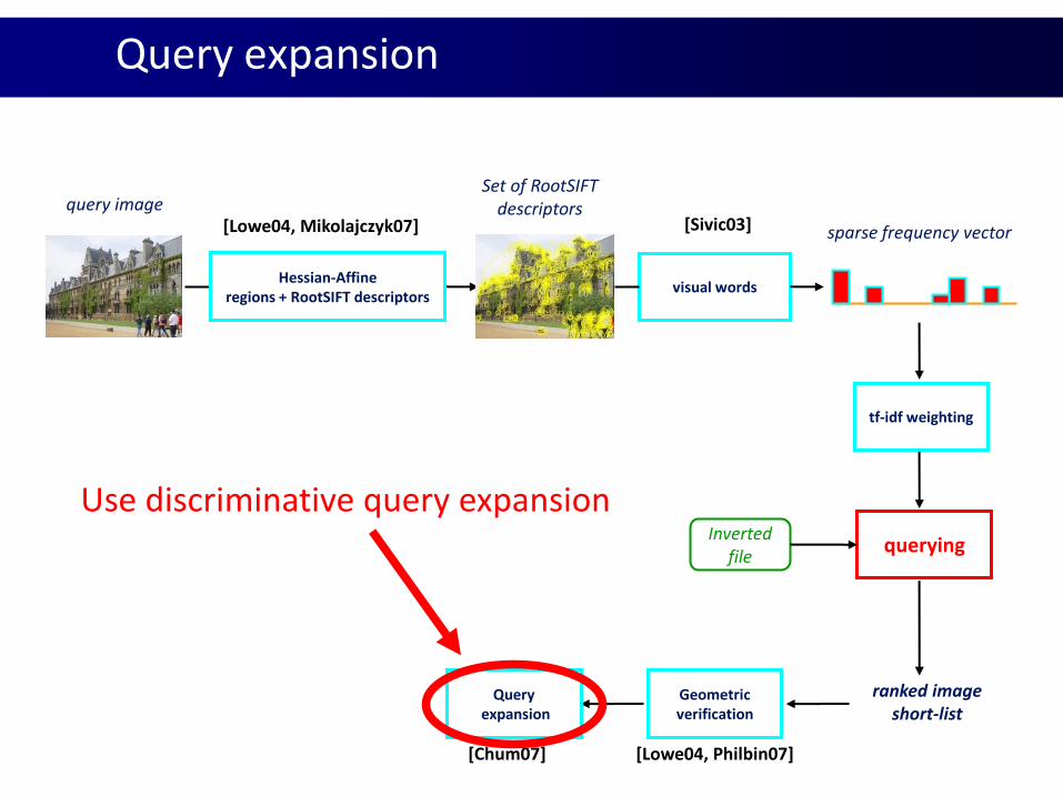
[Lowe04, Philbin07][Chum07]
Hessian-Affineregions + RootSIFT descriptors
visual words
querying
sparse frequency vector
Invertedfile
ranked imageshort-list
Set of RootSIFTdescriptorsquery image
Geometricverification
Queryexpansion
[Lowe04, Mikolajczyk07] [Sivic03]
tf-idf weighting
Query expansion
Use discriminative query expansion
Discriminative Query Expansion: results
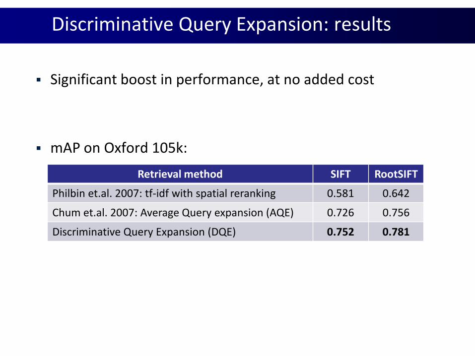
Significant boost in performance, at no added cost
mAP on Oxford 105k:
Retrieval method SIFT RootSIFT
Philbin et.al. 2007: tf-idf with spatial reranking 0.581 0.642
Chum et.al. 2007: Average Query expansion (AQE) 0.726 0.756
Discriminative Query Expansion (DQE) 0.752 0.781
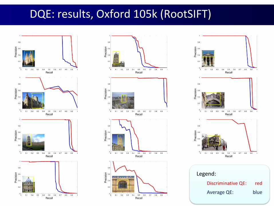
DQE: results, Oxford 105k (RootSIFT)
Legend:
Discriminative QE: red
Average QE: blue
Third thing everyone should know
1. RootSIFT
2. Discriminative query expansion
3. Database-side feature augmentation
Database-side feature augmentation
Query expansion improves retrieval performance by obtaining
a better model for the query
Natural complement: obtain a better model for the database
images [Turcot09]
Augment database images with features from other images of the same
object
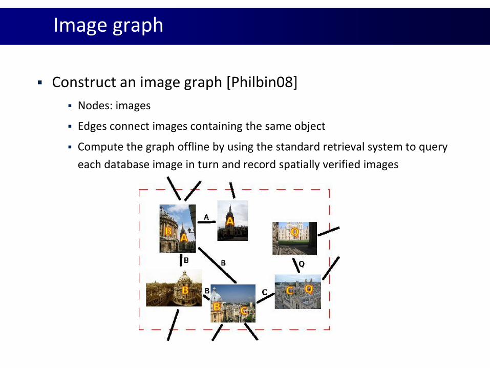
Image graph
Construct an image graph [Philbin08]
Nodes: images
Edges connect images containing the same object
Compute the graph offline by using the standard retrieval system to query
each database image in turn and record spatially verified images
Database-side feature augmentation (AUG)
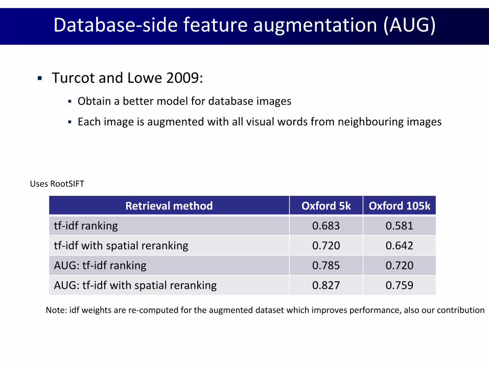
Turcot and Lowe 2009:
Obtain a better model for database images
Each image is augmented with all visual words from neighbouring images
Retrieval method Oxford 5k Oxford 105k
tf-idf ranking 0.683 0.581
tf-idf with spatial reranking 0.720 0.642
AUG: tf-idf ranking 0.785 0.720
AUG: tf-idf with spatial reranking 0.827 0.759
Note: idf weights are re-computed for the augmented dataset which improves performance, also our contribution
Uses RootSIFT
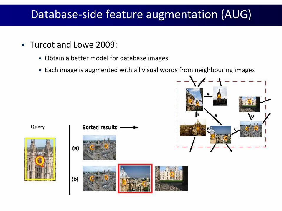
Database-side feature augmentation (AUG)
Turcot and Lowe 2009:
Obtain a better model for database images
Each image is augmented with all visual words from neighbouring images
Query
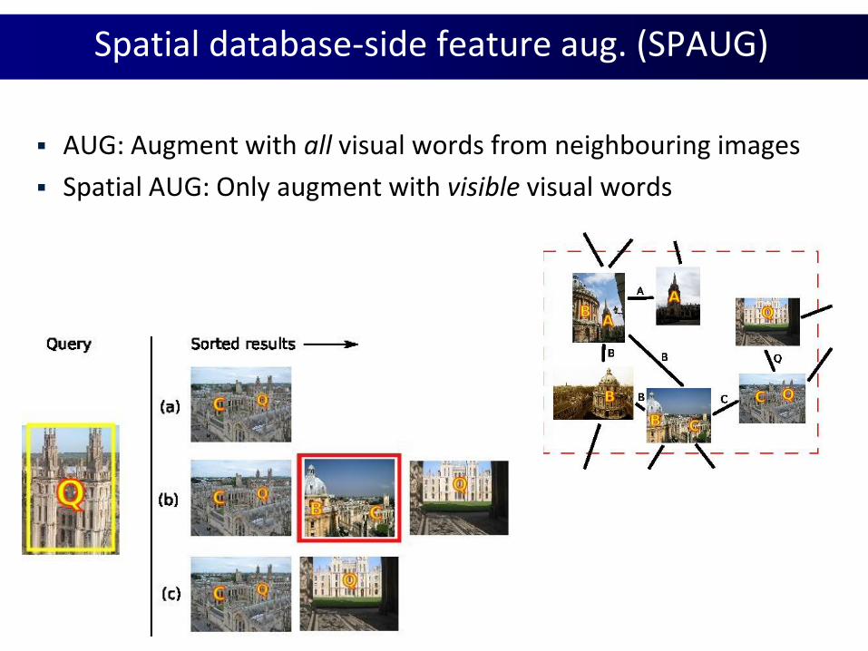
Spatial database-side feature aug. (SPAUG)
AUG: Augment with all visual words from neighbouring images
Spatial AUG: Only augment with visible visual words
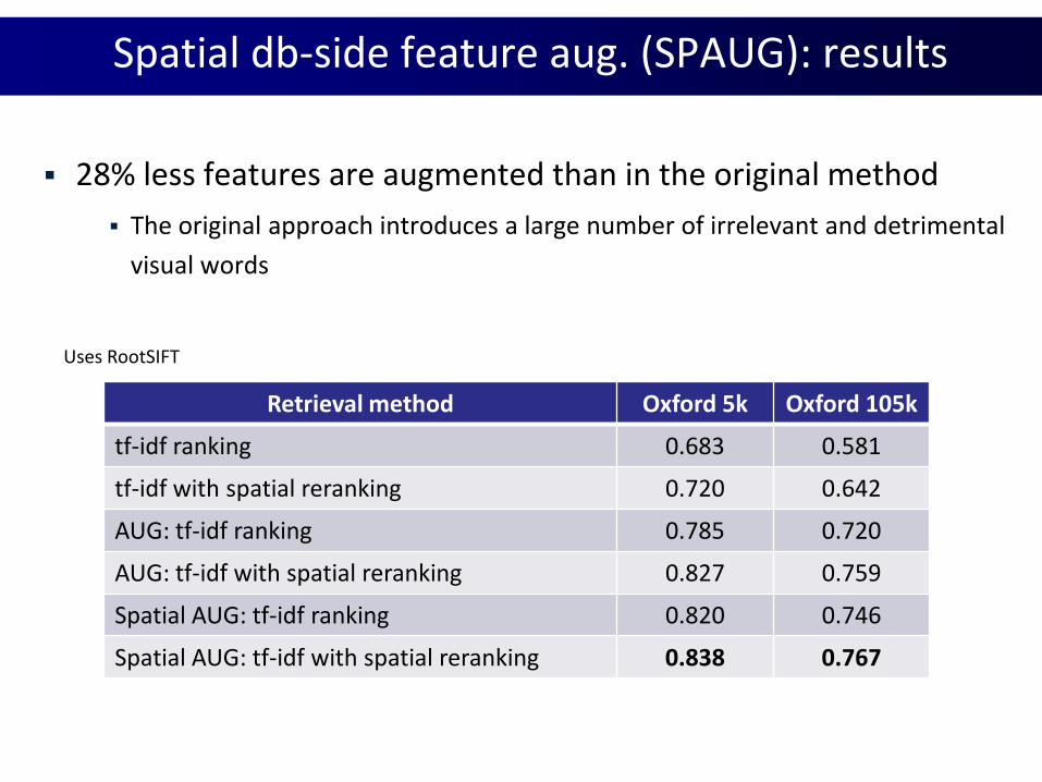
Spatial db-side feature aug. (SPAUG): results
Retrieval method Oxford 5k Oxford 105k
tf-idf ranking 0.683 0.581
tf-idf with spatial reranking 0.720 0.642
AUG: tf-idf ranking 0.785 0.720
AUG: tf-idf with spatial reranking 0.827 0.759
Spatial AUG: tf-idf ranking 0.820 0.746
Spatial AUG: tf-idf with spatial reranking 0.838 0.767
Uses RootSIFT
28% less features are augmented than in the original method
The original approach introduces a large number of irrelevant and detrimental
visual words
Spatial AUG vs AUG
Negative:
The original method does not need to explicitly augment images, it is
equivalent to sum tf-idf scores of neighbouring images at runtime
Spatial database-side feature augmentation has to explicitly augment
images, thus storage requirements are increased significantly
Positive:
While achieving high recall of the original method, precision is
improved
Final retrieval system
Combine all the improvements into one system
RootSIFT
Discriminative query expansion
Spatial database-side feature augmentation
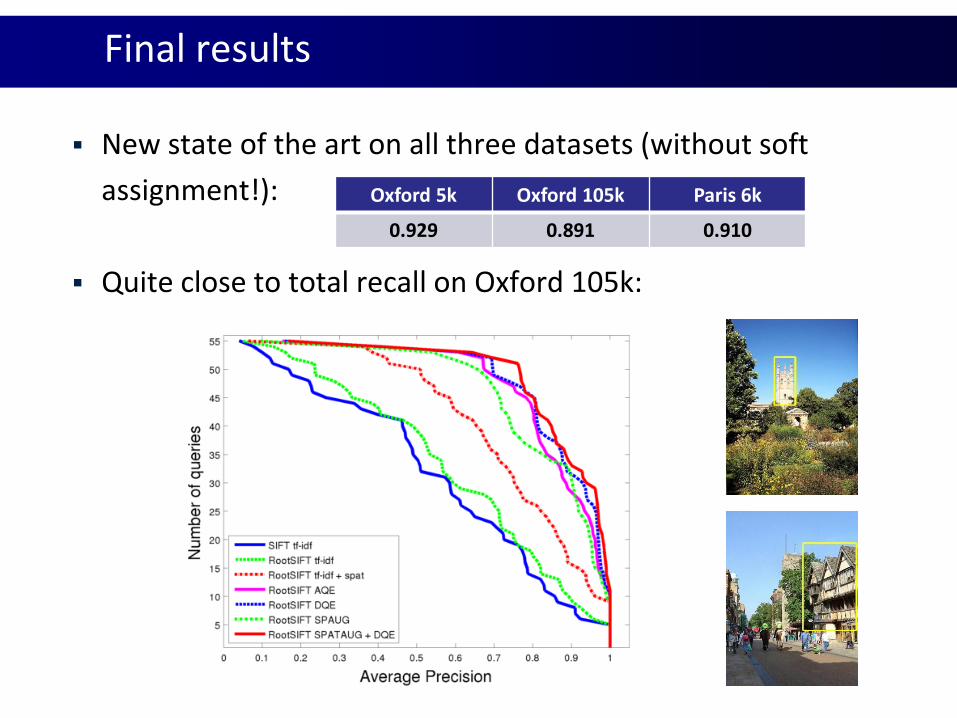
Final results
New state of the art on all three datasets (without soft
assignment!):
Quite close to total recall on Oxford 105k:
Oxford 5k Oxford 105k Paris 6k
0.929 0.891 0.910
Summary
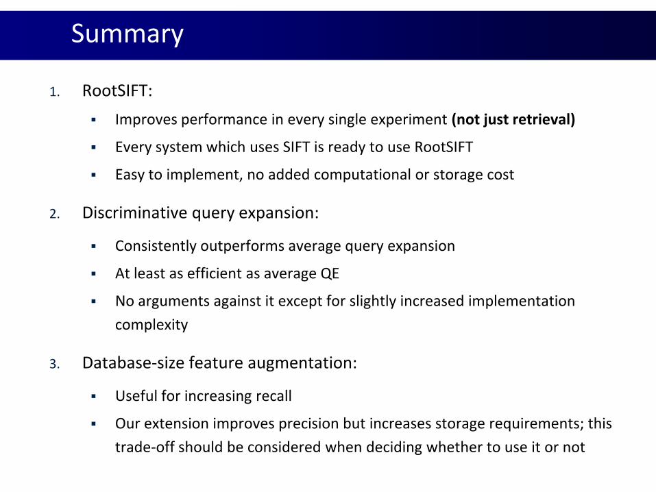
1. RootSIFT:
Improves performance in every single experiment (not just retrieval)
Every system which uses SIFT is ready to use RootSIFT
Easy to implement, no added computational or storage cost
2. Discriminative query expansion:
Consistently outperforms average query expansion
At least as efficient as average QE
No arguments against it except for slightly increased implementation
complexity
3. Database-size feature augmentation:
Useful for increasing recall
Our extension improves precision but increases storage requirements; this
trade-off should be considered when deciding whether to use it or not
Recommended