Time Series Analysis in dplR
Andy Bunn Mikko Korpela
Processed with dplR 1.6.8 in R version 3.5.0 (2018-04-23) on May 23, 2018
Abstract
In this vignette we cover some of the basic time series tools in dplR(and in R to a much lesser extent). These include spectral analysisusing redfit and wavelets. We also discuss fitting AR and ARMA.
Contents
1 Introduction 21.1 What Is Covered . . . . . . . . . . . . . . . . . . . . . . . . . 21.2 Citing dplR and R . . . . . . . . . . . . . . . . . . . . . . . . 2
2 Data Sets 3
3 Characterizing the Data 5
4 Frequency Domain 8
5 Conclusion 13
1
1 Introduction
1.1 What Is Covered
The Dendrochronology Program Library in R (dplR) is a package for den-drochronologists to handle data processing and analysis. This documentgives an introduction of some of the functions dealing with time series indplR. This vignette does not purport to be any sort of authority on timeseries analysis at all! There are many wonderful R-centric books on timeseries analysis that can tell you about the theory and practice of workingwith temporal data. For heaven’s sake, do not rely on this document!
1.2 Citing dplR and R
The creation of dplR is an act of love. We enjoy writing this software andhelping users. However, neither of us is among the idle rich. Alas. Wehave jobs and occasionally have to answer to our betters. There is a niftycitation function in R that gives you information on how to best cite Rand, in many cases, its packages. We ask that you please cite dplR andR appropriately in your work. This way when our department chairs anddeans accuse us of being dilettantes we can point to the use of dplR as apartial excuse.
> citation()
To cite R in publications use:
R Core Team (2018). R: A language and environment
for statistical computing. R Foundation for
Statistical Computing, Vienna, Austria. URL
https://www.R-project.org/.
A BibTeX entry for LaTeX users is
@Manual{,
title = {R: A Language and Environment for Statistical Computing},
author = {{R Core Team}},
organization = {R Foundation for Statistical Computing},
address = {Vienna, Austria},
year = {2018},
url = {https://www.R-project.org/},
}
We have invested a lot of time and effort in creating
R, please cite it when using it for data analysis. See
also 'citation("pkgname")' for citing R packages.
2

> citation("dplR")
Bunn AG (2008). "A dendrochronology program library in
R (dplR)." _Dendrochronologia_, *26*(2), 115-124. ISSN
1125-7865, doi: 10.1016/j.dendro.2008.01.002 (URL:
http://doi.org/10.1016/j.dendro.2008.01.002).
Bunn AG (2010). "Statistical and visual crossdating in
R using the dplR library." _Dendrochronologia_,
*28*(4), 251-258. ISSN 1125-7865, doi:
10.1016/j.dendro.2009.12.001 (URL:
http://doi.org/10.1016/j.dendro.2009.12.001).
Andy Bunn, Mikko Korpela, Franco Biondi, Filipe
Campelo, Pierre Merian, Fares Qeadan, Christian
Zang, Darwin Pucha-Cofrep and Jakob Wernicke (2018).
dplR: Dendrochronology Program Library in R. R
package version 1.6.8.
https://r-forge.r-project.org/projects/dplr/
To see these entries in BibTeX format, use
'print(<citation>, bibtex=TRUE)', 'toBibtex(.)', or
set 'options(citation.bibtex.max=999)'.
2 Data Sets
Throughout this vignette we will use the onboard data set co021 which givesthe raw ring widths for Douglas fir Pseudotsuga menziesii at Mesa Verde inColorado, USA. There are 35 series spanning 788 years.
It is a beautifully sensitive series with long segment lengths, high stan-dard deviation (relative to ring widths), large first-order autocorrelation,and a high mean interseries correlation (r ≈ 0.84). The data are plotted inFigure 1.
> library(dplR)
> data(co021)
> co021.sum <- summary(co021)
> mean(co021.sum$year)
[1] 564.9143
> mean(co021.sum$stdev)
[1] 0.3231714
3

> mean(co021.sum$median)
[1] 0.3211429
> mean(co021.sum$ar1)
[1] 0.6038
> mean(interseries.cor(co021)[, 1])
[1] 0.8477981
> plot(co021, plot.type="spag")
Year
646118
642143
645100
642114
644143
642121
641114
643114
644222
644233
642211
642244
645232
643244
645221
646233
643211
646222
646107
643143
641143
641121
641132
645102
645103
644244
644211
642233
642222
645214
646211
646244
645243
643233
643222
1200 1400 1600 1800
1200 1400 1600 1800
Figure 1: A spaghetti plot of the Mesa Verde ring widths.
By the way, if this is all new to you – you should proceed imme-diately to a good primer on dendrochronology like Fritts (2001).
4

This vignette is not intended to teach you about how to do tree-ring analysis. It is intended to teach you how to use the package.
Let us make a mean-value chronology of the co021 data after detrendingeach series with a frequency response of 50% at a wavelength of 2/3 of eachseries’s length. The chronology is plotted in Figure 2.
> co021.rwi <- detrend(co021, method="Spline")
> co021.crn <- chron(co021.rwi, prefix="MES")
> plot(co021.crn, add.spline=TRUE, nyrs=64)
Time
RW
I
05
1015
2025
30S
ampl
e D
epth
1200 1400 1600 1800
0.0
0.5
1.0
1.5
2.0
1200 1400 1600 1800
Figure 2: The Mesa Verde chronology.
3 Characterizing the Data
Let’s start with a quick exploratory data analysis into the time-series process.The co021.crn object has two columns, the first giving the chronology and
5

the second the sample depth during that year. We will start our analysison the chronology by looking at its autocorrelation structure using R’s acf
and pacf functions.
> dat <- co021.crn[, 1]
> op <- par(no.readonly = TRUE) # Save to reset on exit
> par(mfcol=c(1, 2))
> acf(dat)
> pacf(dat)
> par(op)
0 5 10 20
0.0
0.2
0.4
0.6
0.8
1.0
Lag
AC
F
Series dat
0 5 10 20
−0.
050.
000.
050.
100.
150.
200.
25
Lag
Par
tial A
CF
Series dat
Figure 3: ACF and PACF plots of the Mesa Verde chronology.
The ACF function indicates significant autocorrelation out to a lag of about10 years (which is not uncommon in tree-ring data) while the PACF plotsuggests that the persistence after lag 4 is due to the propagation of theautocorrelation at earlier lags (Figure 3). And one could very well argue
6
that the best model here is an AR(2) model given the marginal significanceof the PACF value at lags 3 and 4. After all, you can get three opinions byasking one statistician to look a time series. But we digress.
We now have the first bit of solid information about the time-seriesproperties of these data, it looks like they fit an AR(4) model. But, R beingR, there are many other ways to check this. The easiest way is to use the ar
function which fits an autoregressive model and selects the order by AIC.
> dat.ar <- ar(dat)
> dat.ar
Call:
ar(x = dat)
Coefficients:
1 2 3 4
0.1997 0.1484 0.0462 0.0748
Order selected 4 sigma^2 estimated as 0.1884
Indeed, ar produces an AR(4) model. We can do the same sort of analysisby automatically fitting an ARMA model using the auto.arima function inthe package "forecast".
> if (require("forecast", character.only = TRUE) &&
+ packageVersion("forecast") >= "3.6") {
+ dat.arima <- auto.arima(dat, ic="bic")
+ summary(dat.arima)
+ head(residuals(dat.arima))
+ coef(dat.arima)
+ acf(residuals(dat.arima),plot=FALSE)
+ }
Series: dat
ARIMA(1,0,1) with non-zero mean
Coefficients:
ar1 ma1 mean
0.8272 -0.6339 0.9740
s.e. 0.0495 0.0684 0.0325
sigma^2 estimated as 0.1875: log likelihood=-457.13
AIC=922.25 AICc=922.3 BIC=940.93
Training set error measures:
7
ME RMSE MAE MPE
Training set 7.679478e-05 0.4321663 0.3426744 -457.9301
MAPE MASE ACF1
Training set 481.3235 0.7941686 -0.0004114487
Autocorrelations of series 'residuals(dat.arima)', by lag
0 1 2 3 4 5 6 7
1.000 0.000 0.021 -0.037 0.005 -0.010 0.023 0.019
8 9 10 11 12 13 14 15
-0.011 0.006 0.044 -0.037 0.032 0.000 -0.068 0.019
16 17 18 19 20 21 22 23
-0.015 0.021 -0.094 0.028 -0.018 -0.024 0.058 0.036
24 25 26 27 28
0.013 0.013 -0.011 -0.030 0.010
Instead of an AR(4) model, auto.arima went for an ARMA(1,1) model –or an ARIMA(1,0,1). The parsimony principle certainly likes a nice simpleARMA(1,1) model. Note that we could look at the residuals (just the firstfew), model coefficients, etc. quite easily. And indeed the residuals are quiteclean as we would expect.
4 Frequency Domain
There is, at times, an almost manic desire to better characterize the spectralaspects of a tree-ring series. In dplR, we’ve implemented two of the mostcommon ways that dendrochronologists go about this and there are a hostof other approaches in R that we won’t get to in this vignette.
The redfit function in dplR is a port of Schulz’s REDFIT (version 3.8e)program and estimates the red-noise spectra of a time series.
> redf.dat <- redfit(dat, nsim = 1000)
> par(tcl = 0.5, mar = rep(2.2, 4), mgp = c(1.1, 0.1, 0))
> plot(redf.dat[["freq"]], redf.dat[["gxxc"]],
+ ylim = range(redf.dat[["ci99"]], redf.dat[["gxxc"]]),
+ type = "n", ylab = "Spectrum (dB)", xlab = "Frequency (1/yr)",
+ axes = FALSE)
> grid()
> lines(redf.dat[["freq"]], redf.dat[["gxxc"]], col = "#1B9E77",lwd=2)
> lines(redf.dat[["freq"]], redf.dat[["ci99"]], col = "#D95F02")
> lines(redf.dat[["freq"]], redf.dat[["ci95"]], col = "#7570B3")
> lines(redf.dat[["freq"]], redf.dat[["ci90"]], col = "#E7298A")
> freqs <- pretty(redf.dat[["freq"]])
> pers <- round(1 / freqs, 2)
8

> axis(1, at = freqs, labels = TRUE)
> axis(3, at = freqs, labels = pers)
> mtext(text = "Period (yr)", side = 3, line = 1.1)
> axis(2); axis(4)
> legend("topright", c("dat", "CI99", "CI95", "CI90"), lwd = 2,
+ col = c("#1B9E77", "#D95F02", "#7570B3", "#E7298A"),
+ bg = "white")
> box()
> par(op)
Frequency (1/yr)
Spe
ctru
m (
dB)
0.0 0.1 0.2 0.3 0.4 0.5
Inf 10 5 3.33 2.5 2Period (yr)
0.0
0.5
1.0
1.5
2.0
2.5
3.0
0.0
0.5
1.0
1.5
2.0
2.5
3.0
datCI99CI95CI90
Figure 4: Spectra of Mesa Verde chronology using redfit
Using the Mesa Verde chronology we see that there are frequencies inthat time series that are significantly different from a red-noise assumptionin the interannual (<3 years) and at low frequencies (multidecadal). Theseare plotted in Figure 4.
9
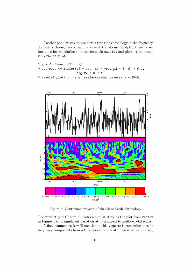
Another popular way to visualize a tree-ring chronology in the frequencydomain is through a continuous wavelet transform. In dplR, there is arefunctions for calculating the transform via wavelet and plotting the resultvia wavelet.plot.
> yrs <- time(co021.crn)
> out.wave <- morlet(y1 = dat, x1 = yrs, p2 = 8, dj = 0.1,
+ siglvl = 0.99)
> wavelet.plot(out.wave, useRaster=NA, reverse.y = TRUE)
0.0000 0.0056 0.0343 0.0733 0.1242 0.1870 0.2760 0.4038 0.6326 1.0025 3.1423
Power2
1200 1400 1600 1800256
128
64
32
16
8
4
2
Time
Per
iod
1200 1400 1600 1800
0.5
1.0
1.5
2.0
2.5
RW
I
Figure 5: Continuous wavelet of the Mesa Verde chronology
The wavelet plot (Figure 5) shows a similar story as the plot from redfit
in Figure 4 with significant variation at interannual to multidecadal scales.A final common task we’ll mention in this vignette is extracting specific
frequency components from a time series to look at different aspects of say,
10

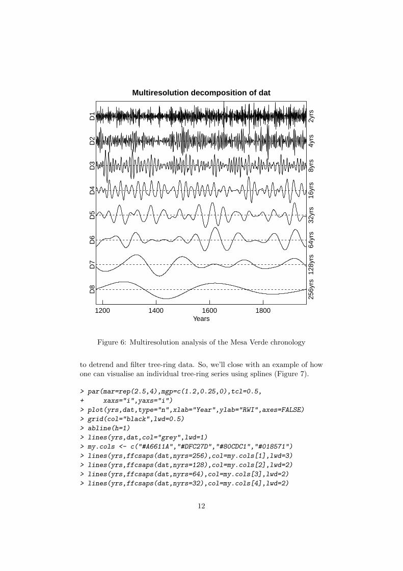
high vs low frequency growth. One approach to doing this is to use waveletsagain but here we will decompose a time series into its constituent voicesusing the mra function in the package "waveslim".
> if (require("waveslim", character.only = TRUE)) {
+ nYrs <- length(yrs)
+ nPwrs2 <- trunc(log(nYrs)/log(2)) - 1
+ dat.mra <- mra(dat, wf = "la8", J = nPwrs2, method = "modwt",
+ boundary = "periodic")
+ YrsLabels <- paste(2^(1:nPwrs2),"yrs",sep="")
+
+ par(mar=c(3,2,2,2),mgp=c(1.25,0.25,0),tcl=0.5,
+ xaxs="i",yaxs="i")
+ plot(yrs,rep(1,nYrs),type="n", axes=FALSE, ylab="",xlab="",
+ ylim=c(-3,38))
+ title(main="Multiresolution decomposition of dat",line=0.75)
+ axis(side=1)
+ mtext("Years",side=1,line = 1.25)
+ Offset <- 0
+ dat.mra2 <- scale(as.data.frame(dat.mra))
+ for(i in nPwrs2:1){
+ # x <- scale(dat.mra[[i]]) + Offset
+ x <- dat.mra2[,i] + Offset
+ lines(yrs,x)
+ abline(h=Offset,lty="dashed")
+ mtext(names(dat.mra)[[i]],side=2,at=Offset,line = 0)
+ mtext(YrsLabels[i],side=4,at=Offset,line = 0)
+ Offset <- Offset+5
+ }
+ box()
+ par(op) #reset par
+ }
In Figure 6 the Mesa Verde chronology is shown via an additive decom-position for each power of 2 from 21 to 28. Note that each voice is scaledto itself by dividing by its standard deviation in order to present them onthe same y-axis. If the scale function were to be removed (and we leavethat as an exercise to the reader) the variations between voices would begreatly reduced. Note the similarity in Figures 5 and 6 for the variation inthe 64-year band around the year 1600 and the lower frequency variation at128 years around the year 1400.
The pioneering work of Ed Cook – e.g. Cook et al. (1990) – has left anenduring mark on nearly every aspect of quantitative dendrochronology. Onesuch mark that we already alluded to above is the use of smoothing splines
11
Multiresolution decomposition of dat
1200 1400 1600 1800Years
D8
256y
rs
D7
128y
rs
D6
64yr
s
D5
32yr
s
D4
16yr
s
D3
8yrs
D2
4yrs
D1
2yrs
Figure 6: Multiresolution analysis of the Mesa Verde chronology
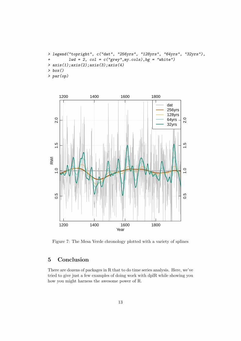
to detrend and filter tree-ring data. So, we’ll close with an example of howone can visualise an individual tree-ring series using splines (Figure 7).
> par(mar=rep(2.5,4),mgp=c(1.2,0.25,0),tcl=0.5,
+ xaxs="i",yaxs="i")
> plot(yrs,dat,type="n",xlab="Year",ylab="RWI",axes=FALSE)
> grid(col="black",lwd=0.5)
> abline(h=1)
> lines(yrs,dat,col="grey",lwd=1)
> my.cols <- c("#A6611A","#DFC27D","#80CDC1","#018571")
> lines(yrs,ffcsaps(dat,nyrs=256),col=my.cols[1],lwd=3)
> lines(yrs,ffcsaps(dat,nyrs=128),col=my.cols[2],lwd=2)
> lines(yrs,ffcsaps(dat,nyrs=64),col=my.cols[3],lwd=2)
> lines(yrs,ffcsaps(dat,nyrs=32),col=my.cols[4],lwd=2)
12
> legend("topright", c("dat", "256yrs", "128yrs", "64yrs", "32yrs"),
+ lwd = 2, col = c("grey",my.cols),bg = "white")
> axis(1);axis(2);axis(3);axis(4)
> box()
> par(op)
Year
RW
I
dat256yrs128yrs64yrs32yrs
1200 1400 1600 1800
0.5
1.0
1.5
2.0
1200 1400 1600 1800
0.5
1.0
1.5
2.0
Figure 7: The Mesa Verde chronology plotted with a variety of splines
5 Conclusion
There are dozens of packages in R that to do time series analysis. Here, we’vetried to give just a few examples of doing work with dplR while showing youhow you might harness the awesome power of R.
13

References
Cook E, Briffa K, Shiyatov S, Mazepa V (1990). “Tree-Ring Standardizationand Growth-Trend Estimation.” In E Cook, L Kairiukstis (eds.), Methodsof Dendrochronology: Applications in the Environmental Sciences, pp.104–123. Kluwer, Dordrecht. ISBN 978-0792305866.
Fritts HC (2001). Tree Rings and Climate. The BlackburnPress. ISBN 1930665393. URL http://www.amazon.com/
Tree-Rings-Climate-H-Fritts/dp/1930665393.
14
Recommended