INTERNATIONAL JOURNAL OF OPTIMIZATION IN CIVIL ENGINEERING
Int. J. Optim. Civil Eng., 2017; 7(3):393-411
TOWER CRANES AND SUPPLY POINTS LOCATING
PROBLEM USING CBO, ECBO, AND VPS
A. Kaveh*, † and Y. Vazirinia
Centre of Excellence for Fundamental Studies in Structural Engineering, Iran University of
Science and Technology, Narmak, Tehran, P.O. Box 16846-13114, Iran
ABSTRACT
Tower cranes are major and expensive equipment that are extensively used at building
construction projects and harbors for lifting heavy objects to demand points. The tower
crane locating problem to position a tower crane and supply points in a building construction
site for supplying all requests in minimum time, has been raised from more than twenty
years ago. This problem has already been solved by linear programming, but meta-heuristic
methods spend less time to solving the problem. Hence, in this paper three newly developed
meta-heuristic algorithms called CBO, ECBO, and VPS have been used to solve the tower
crane locating problem. Three scenarios are studied to show the applicability and
performance of these meta-heuristics.
Keywords: tower crane locating problem; colliding bodies optimization; vibrating particle
system; construction site layout planning; project planning and design.
Received: 10 September 2016; Accepted: 2 February 2017
1. INTRODUCTION
Every construction project needs enough spaces for temporary facilities in order to perform
the construction activities in a safe and efficient manner. Construction site-level facilities
layout is an important step in site planning. Planning construction site spaces to allow for
safe and efficient working status is a complex and multi-disciplinary task as it involves
accounting for a wide range of scenarios. Construction site layout problems are known as
combinatorial optimization problems. There are two types of procedures for solution
consisting of meta-heuristics for large search sized problems and the exact method with
global search for smaller search sized problems [1]. For example, Li and Love [2] developed
a construction site-level facility layout problem for allocating a a set of predetermined
*Corresponding author: Centre of Excellence for Fundamental Studies in Structural Engineering, Iran
University of Science and Technology, Narmak, Tehran, P.O. Box 16846-13114, Iran †E-mail address: [email protected] (A. Kaveh)
Dow
nloa
ded
from
ijoc
e.iu
st.a
c.ir
at 2
0:30
IRD
T o
n F
riday
Aug
ust 3
rd 2
018

A. Kaveh and Y. Vazirinia
394
facilities into a set of predetermined locations, while satisfying the layout constraints and
requirements. They used a genetic algorithm to solve the problem by assuming that the
predetermined locations are in rectangular shape and are large enough to accommodate the
largest facility. Gharaie et al. [3] resolved their model by Ant Colony Optimization, and
Kaveh et al. [4] used Colliding Bodies Optimization and its enhanced version. Similarly,
Cheung et al. [5] have developed another model for construction site layout planning and
solved it by Genetic Algorithm. Also Liang and Chao [6], Wong et al. [7], Kaveh et al. [8],
and Kaveh et al. [4] have employed Multi-searching tabu search, Mixed Integer
Programming, and CBO, ECBO, and PSO, respectively.
The tower crane is an important facility used in the vertical and horizontal transportation
of materials, particularly heavy prefabrication units such as steel beams, ready-mixed
concrete, prefabricated elements, and large-panel formworks [9]. The Tower Crane Locating
Problem to positioning a tower crane and supply points in a building construction site for
supplying all the requests in a minimum time, has been raised more than twenty years ago.
An analytical model was developed by Zhang et al. [10] considering the travel time of tower
crane hooks and adopting a Monte Carlo simulation to optimize the tower crane location.
However, considered tower crane in their study was a single one and the effect of location of
supply points on lifting requirements and travel time has been neglected. Tam et al. [9]
employed an artificial neural network model for predicting tower crane operations and next
they used a genetic algorithm model to optimize the crane and supply points layout [9] and
[11]. The case study used by Tam et al. [11] to show the effectiveness of their model was
subsequently used in a number of researches to compare the effectiveness of other
optimization methods. For example, Huang et al. [1] used mixed integer linear programming
(MILP) to optimize the crane and supply locations and showed that their method reduced the
travel time of the hook by 7% compared to the results obtained from the previous genetic
algorithm. MILP was used to ensure achieving a global optimal solution [1]. In this research,
we use new meta-heuristic techniques, because they require less computational time to
solving the problem.
Solving real-life problems by meta-heuristic algorithms has become to an interesting
topic in recent years. Many meta-heuristics with different philosophy and characteristics are
developed and applied to a wide range of fields. The aim of these optimization methods is to
efficiently explore the search space in order to find global or near-global solutions. Since
these algorithms are not problem specific and do not require the derivatives of the objective
function, they have received increasing attention from both academia and industry [12].
Meta-heuristic methods are global optimization methods that try to reproduce natural
phenomena (Genetic Algorithm [13], Particle Swarm Optimization [14], Water Evaporation
Optimization [15]), humans social behavior (Imperialist Competitive Algorithm[16]), or
physical phenomena (Charged System Search (CSS) [17], Colliding Bodies Optimization
[18], Big Bang-Big Chrunch [19], Vibrating Particle System (VPS) [12]). Exploitation and
exploration are two important characteristics of meta-heuristic optimization methods, Kaveh
[20]. Exploitation serves to search around the current best solutions and to select the best
possible points, and Exploration allows the optimizer to explore the search space more
efficiently, often by randomization.
In this paper three newly developed meta-heuristics named: Colliding Bodies
Optimization (CBO), Enhanced Colliding Bodies Optimization (ECBO) [21], and Vibrating
Dow
nloa
ded
from
ijoc
e.iu
st.a
c.ir
at 2
0:30
IRD
T o
n F
riday
Aug
ust 3
rd 2
018

Tower cranes and supply points locating problem using CBO, ECBO, and VPS
395
Particle System (VPS) [12] are used for tower crane and material supply locating model that
proposed by Huang et al. [1] and results are discussed.
2. OPTIMIZATION ALGORITHMS
2.1 Colliding bodies optimization
An efficient algorithm, inspired from the momentum, and energy rules of the physics, named
Colliding Bodies Optimization, that was developed by Kaveh and Mahdavi [18]. CBO does
not depend on any internal parameter and also it is extremely simple in the sense. In this
method, one body collides by another body and they moves to the lower cost. Each solution
candidate “X” at CBO, contains a number of variables and is considered
as a colliding body (CB). The massed bodies are divided in two main equal groups; i.e.,
stationary and moving bodies (Fig. 2), where the moving bodies moves to stationary bodies
and a collision occurs between the pairs of bodies. The goal of this process is: (i) to improve
the locations of moving bodies and (ii) to push stationary bodies toward the better locations.
After the collision, new locations of colliding bodies are updated based on the new velocity
by using the collision rules. The main procedure of the CBO is described as:
Step 1: The initial positions of colliding bodies are determined with random initialization
of a population of individuals in the search space:
(1)
where, determines the initial value vector of the ith colliding body. are the
minimum and the maximum allowable values vectors of variables, respectively; rand is a
random number in the interval ; and n is the number of colliding bodies.
Step 2: The magnitude of the body mass for each colliding body is defined as:
(2)
where fit (i) represents the objective function value of the colliding body i; n is the
population size. It seems that a colliding body with good values exerts a larger mass than the
bad ones. Also, for maximization, the objective function will be replaced by .
Step 3: Then colliding bodies objective function values are arranged in an ascending
order. The sorted colliding bodies are divided into two equal groups:
The lower half of the CBs (stationary CBs); These CBs are good agents which are
stationary and the velocity of these bodies before collision is zero. Thus:
(3)
The upper half of CBs (moving CBs): These CBs move toward the lower half. Then,
according to Fig. 1, the better and worse CBs, i.e. agents with upper fitness value, of each
Dow
nloa
ded
from
ijoc
e.iu
st.a
c.ir
at 2
0:30
IRD
T o
n F
riday
Aug
ust 3
rd 2
018

A. Kaveh and Y. Vazirinia
396
group will collide together. The change of the body position represents the velocity of
these bodies before collision as:
(4)
where, and are the velocity and position vector of the ith CB in this group, respectively;
is the ith CB pair position of in the previous group.
Figure 1. Pairs of CBs for collision
Step 4: After the collision, the velocities of the CBs in each group are evaluated as:
Stationary CBs:
(5)
Moving CBs:
(6)
where ε is the Coefficient Of Restitution (COR) of the two colliding bodies, defined as:
(7)
with and being the current iteration number and the total number of iteration
for optimization process, respectively.
New positions of CBs are updated using the generated velocities after the collision in
position of stationary CBs, as follow for each group:
Moving CB:
Dow
nloa
ded
from
ijoc
e.iu
st.a
c.ir
at 2
0:30
IRD
T o
n F
riday
Aug
ust 3
rd 2
018

Tower cranes and supply points locating problem using CBO, ECBO, and VPS
397
(8)
where, and
are the new position and the velocity after the collision of the ith moving
CB, respectively;
is the old position of the ith stationary CB pair.
Stationary CB:
(9)
where,
are the new positions, previous positions and the velocity after the
collision of the ith CB, respectively. rand is a random vector uniformly distributed in the
range of [-1,1] and the sign ‘°’ denotes an element-by-element multiplication.
Step 6: The process is repeated from step 2 until one termination criterion is satisfied.
Termination criterion is the predefined maximum number of iterations. After getting the
near-global optimal solution, it is recorded to generate the output.
Pseudo Code of Colliding Bodies Optimization
Initial location is created randomly by Eq. (1)
The value of the objective function is evaluated and masses are defined by Eq. (2)
While stop criteria is not attained (like max iteration)
for each CBs
Calculate Stationary and moving CBs velocity before collision according Eqs. (3)
and (4)
Calculate CBs velocity after collision according by Eqs. (5) and (6)
Update CBs position according Eqs. (8) and (9)
End for
End while
Case 1.End
Figure 2. Pseudo code of the colliding bodies optimization
2.2. Enhanced colliding bodies optimization
In order to improve CBO to get faster and more reliable solutions, Enhanced Colliding
Bodies Optimization (ECBO) was developed which uses memory to save a number of
historically best CBs and also utilizes a mechanism to escape from local optima [11]. The
pseudo of ECBO is shown in Fig. 3 and the steps involved are given as follows:
Step 1: Initialization
Initial positions of all CBs are determined randomly in an m-dimensional search space by
Eq. (1).
Step 2: Defining mass
The value of mass for each CB is evaluated according to Eq. (2).
Step 3: Saving
Considering a memory which saves some historically best CB vectors and their related
mass and objective function values can improve the algorithm performance without
Dow
nloa
ded
from
ijoc
e.iu
st.a
c.ir
at 2
0:30
IRD
T o
n F
riday
Aug
ust 3
rd 2
018

A. Kaveh and Y. Vazirinia
398
increasing the computational cost [16]. For that purpose, a Colliding Memory (CM) is
utilized to save a number of the best-so-far solutions. Therefore in this step, the solution
vectors saved in CM are added to the population, and the same numbers of current worst
CBs are deleted. Finally, CBs are sorted according to their masses in a decreasing order.
Step 4: Creating groups
CBs are divided into two equal groups: (i) stationary group and (ii) moving group. The
pairs of CBs are defined according to Fig. 1.
Step 5: Criteria before the collision
The velocity of stationary bodies before collision is zero (Eq. (3)). Moving objects move
toward stationary objects and their velocities before collision are calculated by Eq. (4).
Step 6: Criteria after the collision
The velocities of stationary and moving bodies are calculated using Eqs. (5) and (6),
respectively.
Step 7: Updating CBs
The new position of each CB is calculated by Eqs. (8) and (9).
Pseudo Code of Enhanced Colliding Bodies Optimization
Initial location is created randomly by Eq. (1)
The value of objective function is evaluated and masses are defined by Eq. (2)
While stop criteria is not attained (like max iteration)
for each CBs
Calculate Stationary and moving CBs velocity before collision according Eqs. (3)
and (4)
Calculate CBs velocity after collision according by Eqs. (5) and (6)
Update CBs position according Eqs. (8) and (9)
If rand i < Pro
One dimension of the ith CB is selected randomly and regenerate by Eq. (10)
End if
End for
End while
End
Figure 3. Pseudo code of the enhanced colliding bodies optimization [24]
Step 8: Escape from local optima
Meta-heuristic algorithms should have the ability to escape from the trap when agents get
close to a local optimum. In ECBO, a parameter like Pro within (0, 1) is introduced and it is
specified whether a component of each CB must be changed or not. For each colliding body
Pro is compared with which is a random number uniformly distributed
within (0, 1). If , one dimension of the ith CB is selected randomly and its value
is regenerated as follows:
(10)
where is the jth variable of the ith CB. and respectively, are the lower and
upper bounds of the jth variable. In order to protect the structures of CBs, only one
Dow
nloa
ded
from
ijoc
e.iu
st.a
c.ir
at 2
0:30
IRD
T o
n F
riday
Aug
ust 3
rd 2
018

Tower cranes and supply points locating problem using CBO, ECBO, and VPS
399
dimension is changed. This mechanism provides opportunities for the CBs to move all over
the search space thus providing better diversity.
Step 9: Terminating condition check
The optimization process is terminated after a fixed number of iterations. If this criterion
is not satisfied go to Step 2 for a new round of iteration.
2.3 Vibrating particle system
The VPS is a population-based algorithm which simulates a free vibration of single degree
of freedom systems with viscous damping [12]. Similar to other multi-agent methods, VPS
has a number of individuals (or particles) consisting of the variables of the problem. In the
VPS each solution candidate is defined as “X”, and contains a number of variables (i.e., Xi =
{ }) and is considered as a particle. Particles are damped based on three equilibrium
positions with different weights, and during each iteration the particle position is updated by
learning from them: (i) the historically best position of the entire population (HB), (ii) a
good particle (GP), and (iii) a bad particle (BP). The solution candidates gradually approach
to their equilibrium positions that are achieved from current population and historically best
position in order to have a proper balance between diversification and intensification. Main
procedure of this algorithm is defined as: Step 1: Initialization
Initial locations of particles are created randomly in an n-dimensional search space, by
Eq. (11):
(11)
where, is the jth variable of the particle i. are respectively the minimum
and the maximum allowable values vectors of variables. rand is a random number in the
interval [0,1]; and n is the number of particles.
Step 2: Evaluation of candidate solutions
The objective function value is calculated for each particle.
Step 3: Updating the particle positions
In order to select the GP and BP for each candidate solution, the current population is
sorted according to their objective function values in an increasing order, and then GP and
BP are chosen randomly from the first and second half, respectively.
According to the above concepts, the particles position are updated by follow equation:
(12)
where is the jth variable of the particle i. 1, 2, 3, are three parameters to measure the
relative importance of HB, GP and BP, respectively ( ). rand1, rand2, and
rand3 are random numbers uniformly distributed in the range of [0, 1] respectively. The
parameter A is defined as:
(13)
Dow
nloa
ded
from
ijoc
e.iu
st.a
c.ir
at 2
0:30
IRD
T o
n F
riday
Aug
ust 3
rd 2
018

A. Kaveh and Y. Vazirinia
400
Parameter D is a descending function based on the number of iterations:
(14)
In order to have a fast convergence in the VPS, the effect of BP is sometimes considered
in updating the position formula. Therefore, for each particle, a parameter like p within (0,1)
is defined, and it is compared with rand (a random number uniformly distributed in the range
of [0,1]) and if p < rand, then = 0 and .
Three essential concepts consisting of self-adaptation, cooperation, and competition are
considered in this algorithm. Particles moves towards HB so the self-adaptation is provided.
Any particle has the chance to have influence on the new position of the other one, so the
cooperation between the particles is supplied. Because of the p parameter, the influence of
GP (good particle) is more than that of BP (bad particle), and therefore the competition is
provided.
Step 4: Handling the side constraints
There is a possibility of boundary violation when a particle moves to its new position. In
the proposed algorithm, for handling boundary constraints a harmony search-based approach
is used [17]. In this technique, there is a possibility like harmony memory considering rate
(HMCR) that specifies whether the violating component must be changed with the
corresponding component of the historically best position of a random particle or it should
be determined randomly in the search space. Moreover, if the component of a historically
best position is selected, there is a possibility like pitch adjusting rate (PAR) that specifies
whether this value should be changed with the neighboring value or not.
Pseudo code of Vibrating Particles System (VPS)
Initialize algorithm parameters
Create initial positions randomly by Eq. (11)
Evaluate the values of objective function and store HB
While maximum iterations is not fulfilled
for each particle
The GP and BP are chosen
if P<rand
W3=0 and w2=1-w1
end if
for each component
New location is obtained by Eq. (12)
end for
Violated components are regenerated by harmony search-based handling approach
end for
end while
The values of objective function are evaluated and HB is updated
end
Figure 4. Pseudo code of the vibrating particles system algorithm [22]
Dow
nloa
ded
from
ijoc
e.iu
st.a
c.ir
at 2
0:30
IRD
T o
n F
riday
Aug
ust 3
rd 2
018

Tower cranes and supply points locating problem using CBO, ECBO, and VPS
401
Step 5: Terminating condition check
Steps 2 through 4 are repeated until a termination criterion is fulfilled. Any terminating
condition can be considered, and in this study the optimization process is terminated after a
fixed number of iterations. Pseudo code of the VPS is showed in Fig. 4.
3. PROBLEM: OPTIMIZATION OF TOWER CRANE LOCATION AND
MATERIAL SUPPLY POINTS
Many researches have been conducted on the locating and transporting time of a tower
crane, such as: Choi and Harris [22] improved a mathematical model for determining the
most suitable tower crane location; Zhang et al. [10] developed the Monte Carlo simulation
approach to optimize tower crane location; Tam and Tong [9] employed an artificial neural
network model for predicting tower crane operations and genetic algorithm model for site
facility layout [9, 11]. Huang et al. [1] developed a mixed integer linear programming
(MILP) to optimize the crane and supply locations were and their model decreased the
travel time of the hook by 7% compared to the results obtained from the previous genetic
algorithm. Travel distance between the supply and demand points can be calculated by the
Eq. (15) through Eq. (19) referring to Figs. 5 and 6.
Rib of the crane
---- Angular movement path of the rib of the
crane (tangent movement)
o Hook position
← Change of hook position (radial movement)
Crane position
Figure 5. Radial and tangent movements of the hook
Figure 6. Vertical movement of the hook
(15)
Dow
nloa
ded
from
ijoc
e.iu
st.a
c.ir
at 2
0:30
IRD
T o
n F
riday
Aug
ust 3
rd 2
018

A. Kaveh and Y. Vazirinia
402
(16)
(17)
(18)
(19)
Hook movement time is an important parameter to evaluate the total time of material
transportation using a tower crane. The hook movement time has split up into horizontal and
vertical paths to reflect the operating costs by giving an appropriate cost-time factor.
Corresponding movement paths along different directions can be seen from Figs. 5 and 6.
A continuous type parameter α indicates the degree of coordination of the hook
movement in radial and tangential directions which depends on the control skills of a tower
crane operator, times for horizontal and vertical hook movements can be calculated in Eqs.
(20) and (21), respectively.
(20)
(21)
The total travel time of tower crane at location k between supply point i and demand
point j, , can be calculated using Eq. (22) by specifying the continuous type parameter ß
for the degree of coordination of hook movement in horizontal and vertical planes.
Depending on different site conditions, skills of operators, or even the visibility level due to
environmental and weathering effects, the movement of the tower crane and the hook
operation may be influenced and overall efficiency can be reduced, meaning that longer
operating time is required for moving the tower crane from one point to another [24]. The
aggregate travel time from the material supply location to the demand point should be
increased accordingly if the operator's line of sight is obstructed. To realize these site
operating difficulties, another numerical parameter is introduced to factor up the original
tower crane and hook travel times given in Eq. (22). Different may be used for different
tower crane locations k to determine the location specific effects within a construction site.
If advance vision system is installed in tower cranes to assist operators, the operation time
can be faster and a smaller can be set [1].
(22)
Huang et al. [1] provided three scenarios to demonstrate the flexibility of their proposed
MILP model of a tower crane location. The formulation will be extended to consider
homogeneous and non-homogeneous storage supply points where different materials can be
stored in different strategies by confining the solution region with extra sets of linear type
governing constraints.
Only one tower crane can be modeled which can be allocated at any one of the available
Dow
nloa
ded
from
ijoc
e.iu
st.a
c.ir
at 2
0:30
IRD
T o
n F
riday
Aug
ust 3
rd 2
018

Tower cranes and supply points locating problem using CBO, ECBO, and VPS
403
locations. Binary variables like are defined for a location k, where if the location k
is selected for a tower crane location or otherwise. Constraint (23) is required, so
only the best tower crane location can be picked in the optimization framework.
(23)
A set of binary variables is introduced to represent the existence of a demand location
where j is the potential demand point. Depending on the input material demand profile
for material type l, constraint set (24) is required to ensure the binary variable to be “1” if
there is a demand at location j and “0” if the demand does not exist. ‘M’ is an arbitrary large
integral number.
(24)
3.1 Homogeneous material supply point
As a management problem, it is worth examining the total cost for transporting all the
required materials to demand points through a tower crane if the materials can be stored and
supplied in more than one location without setting a storage limit on various supply
locations realizing that the supply locations have infinite material storage capacity, which is
always the case in large scale construction sites. Under a homogeneous material supply
system, each supply point provides a temporary material storage that is restricted to supply
only one type of material during construction. In the optimization process, we have to ensure
that only one material type is allocated at a specific supply location.
Mathematically, a set of binary decision variables is defined and controlled by
constraint sets (25) and (26). In Eq. (25), for each material type , where L is the
total number of material types to be considered, there must be one assigned supply location
within a site. Similarly, for each supply location where I is the total number of
available supply points in a site that can store the construction material, at most one material
type can be allocated as given in Eq. (26).
(25)
(26)
Objective function is defined as the total material transportation costs for optimization
and these costs depend on the actual amount of material flows associating with different
supply and demand locations. A set of auxiliary binary variables is thus defined to
represent such existence of material flows which equals to “1” if material type l at supply
point i is transported by a tower crane at location k to a demand point j and “0” otherwise.
With the constraint set (13), the decision variables represent the linkage between
Dow
nloa
ded
from
ijoc
e.iu
st.a
c.ir
at 2
0:30
IRD
T o
n F
riday
Aug
ust 3
rd 2
018

A. Kaveh and Y. Vazirinia
404
material l and supply location i, represent demand location j and represent the
selection of the tower crane kth location. Numerically, if all , and ,
then the linkage of material flow is established giving . And for all other
cases so that no transportation cost will be counted in the objective function.
(27)
With the auxiliary variable expressing the existence of material flows, the total cost
for material transportation from various supply points to demand points by a tower crane can
be calculated using Eq. (28) that can be set as an objective function for optimization in the
present formulation. The total cost TCh is simply defined as the sum of all transportation
costs between supply and demand locations by a tower crane located at location k according
to the set of material flow variables for a homogenous material supply system. In Eq.
(28), Ql,j is the required quantity of material l at demand point j, C is the cost per unit time in
operating a tower crane, and is the actual transport time between supply location i and
demand location j by a tower crane at location k. The total cost can be evaluated and set as
an objective function for optimization in the present formulation.
(28)
Optimization of the tower crane position in a homogeneous material supply system can
be formulated to optimize the objective function in Eq. (28) subject to constraint sets in Eqs.
(15)–(27).
3.2. Non-homogeneous material supply without area size constraint scenario
For larger construction sites in size without much physical size restrictions, the actual space
allocated for material storage areas can be relatively increased. Different material types are
able to be stored at one location (usually requiring larger space). For the case of this non-
homogeneous material supply system, the tower crane operations and movements can be
refined to save crane movement times and costs. To ensure that each potential material
demand location is served, there must be at least one supply point for the required material
types. Mathematically, this can be controlled by a set of binary variable yi,j in the constraint
set (29). In this set, for each actual demand location where J is the total number of
demand location whenever , at least one supply location must be selected and even
one supply point can simultaneously serve for numerous demand locations.
(29)
An auxiliary binary-type variable is newly defined and governed by the constraint
set (30) to establish the links among different supply and demand locations and the tower
Dow
nloa
ded
from
ijoc
e.iu
st.a
c.ir
at 2
0:30
IRD
T o
n F
riday
Aug
ust 3
rd 2
018

Tower cranes and supply points locating problem using CBO, ECBO, and VPS
405
crane position. Numerically, whenever , meaning that a supply location i is linked
with demand location j, and with tower crane location k is selected, then the linkage
must be established that is so that the transportation cost can be calculated.
(30)
The total transportation cost for non-homogeneous supply point TCn is given by Eq. (31)
according to the established material flow linkage . In Eq. (31), is the required
quantity of material type l at a demand point j. C is the unit time cost of operating a tower
crane, and is the actual transport time between supply location i and demand location j by
a tower crane located at position k.
Optimizing of the tower crane position in a non-homogeneous material supply system
can be formulated to optimize the objective function in Eq. (31) subjected to constraint sets
in Eqs. (15)–(24), and (29), (30).
(31)
3.3 Non-homogeneous material supply location with physical size constraint
For the construction sites in the urban areas, work space is very limited and the material
storage areas are comparatively small. In that sense, each material supply point can only
supply construction materials for one demand point within a construction site. Similar to the
previous non-homogeneous material supply strategy, different materials can still be stored at
one material supply location. Mathematically, the binary variable , which is used for
identifying linkages of material supply and demand locations as given in Eq. (29), is
governed by two additional constraint sets in Eqs. (32) and (33). In Eq. (32), for each
demand location where j is the total number of demand locations to be considered,
it must be assigned one supply location to store the materials. Similarly, for each supply
location with i being the total number of available supply location in a site that can
store the construction material. Due to the storage area restriction, each supply location can
only allocate materials for one demand location as given in Eq. (33).
(32)
and
(33)
To optimize the total material transportation cost with these storage area constraints,
the objective function in Eq. (31) can be applied and the problem is subjected to constraint
sets as described in Eqs. (15)–(24), (29), (30), and (32), (33).
Dow
nloa
ded
from
ijoc
e.iu
st.a
c.ir
at 2
0:30
IRD
T o
n F
riday
Aug
ust 3
rd 2
018
A. Kaveh and Y. Vazirinia
406
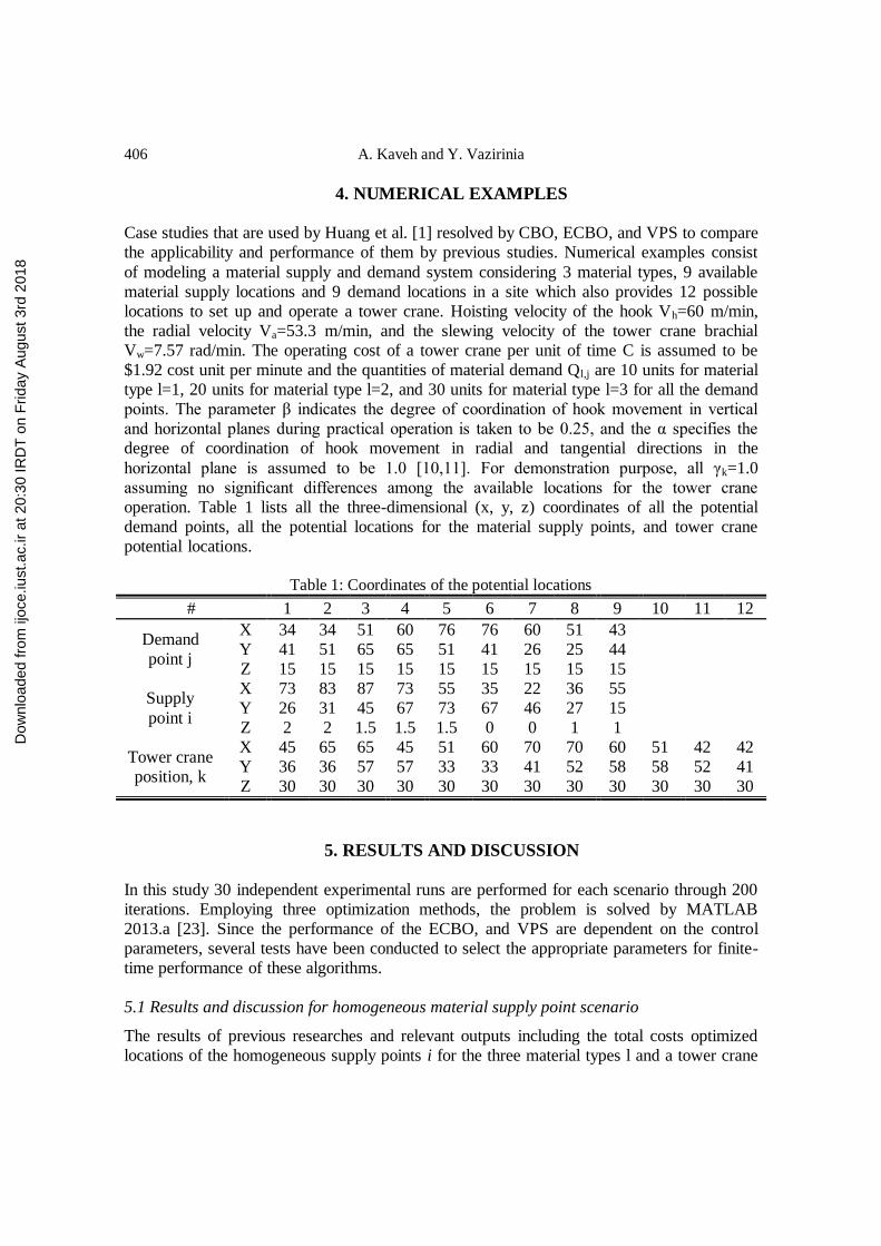
4. NUMERICAL EXAMPLES
Case studies that are used by Huang et al. [1] resolved by CBO, ECBO, and VPS to compare
the applicability and performance of them by previous studies. Numerical examples consist
of modeling a material supply and demand system considering 3 material types, 9 available
material supply locations and 9 demand locations in a site which also provides 12 possible
locations to set up and operate a tower crane. Hoisting velocity of the hook Vh=60 m/min,
the radial velocity Va=53.3 m/min, and the slewing velocity of the tower crane brachial
Vw=7.57 rad/min. The operating cost of a tower crane per unit of time C is assumed to be
$1.92 cost unit per minute and the quantities of material demand Ql,j are 10 units for material
type l=1, 20 units for material type l=2, and 30 units for material type l=3 for all the demand
points. The parameter β indicates the degree of coordination of hook movement in vertical
and horizontal planes during practical operation is taken to be 0.25, and the α specifies the
degree of coordination of hook movement in radial and tangential directions in the
horizontal plane is assumed to be 1.0 [10,11]. For demonstration purpose, all γk=1.0
assuming no significant differences among the available locations for the tower crane
operation. Table 1 lists all the three-dimensional (x, y, z) coordinates of all the potential
demand points, all the potential locations for the material supply points, and tower crane
potential locations.
Table 1: Coordinates of the potential locations
# 1 2 3 4 5 6 7 8 9 10 11 12
Demand
point j
X 34 34 51 60 76 76 60 51 43
Y 41 51 65 65 51 41 26 25 44
Z 15 15 15 15 15 15 15 15 15
Supply
point i
X 73 83 87 73 55 35 22 36 55
Y 26 31 45 67 73 67 46 27 15
Z 2 2 1.5 1.5 1.5 0 0 1 1
Tower crane
position, k
X 45 65 65 45 51 60 70 70 60 51 42 42
Y 36 36 57 57 33 33 41 52 58 58 52 41
Z 30 30 30 30 30 30 30 30 30 30 30 30
5. RESULTS AND DISCUSSION
In this study 30 independent experimental runs are performed for each scenario through 200
iterations. Employing three optimization methods, the problem is solved by MATLAB
2013.a [23]. Since the performance of the ECBO, and VPS are dependent on the control
parameters, several tests have been conducted to select the appropriate parameters for finite-
time performance of these algorithms.
5.1 Results and discussion for homogeneous material supply point scenario
The results of previous researches and relevant outputs including the total costs optimized
locations of the homogeneous supply points i for the three material types l and a tower crane
Dow
nloa
ded
from
ijoc
e.iu
st.a
c.ir
at 2
0:30
IRD
T o
n F
riday
Aug
ust 3
rd 2
018
Tower cranes and supply points locating problem using CBO, ECBO, and VPS
407
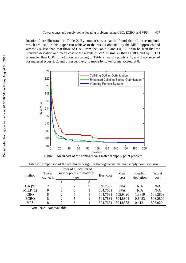
location k are illustrated in Table 2. By comparison, it can be found that all three methods
which are used in this paper can achieve to the results obtained by the MILP approach and
almost 7% less than that those of GA. From the Table 2 and Fig. 8, it can be seen that the
standard deviation and mean cost of the results of VPS is smaller than ECBO, and by ECBO
is smaller than CBO. In addition, according to Table 2, supply points 2, 5, and 1 are selected
for material types 1, 2, and 3, respectively to move by tower crane located at 8.
Figure 8. Mean cost of the homogeneous material supply point problem
Table 2: Comparison of the optimized design for homogeneous material supply point scenario
method Tower
crane, k
Order of allocation of
supply points to material
type Best cost
Mean
cost
Standard
deviation
Worst
cost
1 2 3
GA (9) 2 3 2 9 540.7587 N/A N/A N/A MILP (1) 8 2 5 1 504.7631 N/A N/A N/A
CBO 8 2 5 1 504.7631 505.9426 1.3319 508.2809
ECBO 8 2 5 1 504.7631 504.8804 0.6423 508.2809
VPS 8 2 5 1 504.7631 504.8383 0.4121 507.0204
Note: N/A: Not available
Dow
nloa
ded
from
ijoc
e.iu
st.a
c.ir
at 2
0:30
IRD
T o
n F
riday
Aug
ust 3
rd 2
018
A. Kaveh and Y. Vazirinia
408
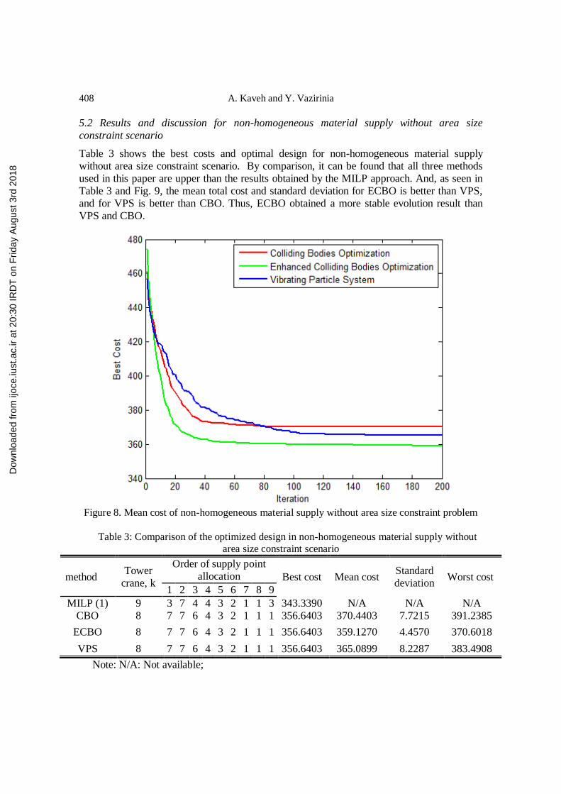
5.2 Results and discussion for non-homogeneous material supply without area size
constraint scenario
Table 3 shows the best costs and optimal design for non-homogeneous material supply
without area size constraint scenario. By comparison, it can be found that all three methods
used in this paper are upper than the results obtained by the MILP approach. And, as seen in
Table 3 and Fig. 9, the mean total cost and standard deviation for ECBO is better than VPS,
and for VPS is better than CBO. Thus, ECBO obtained a more stable evolution result than
VPS and CBO.
Figure 8. Mean cost of non-homogeneous material supply without area size constraint problem
Table 3: Comparison of the optimized design in non-homogeneous material supply without
area size constraint scenario
method Tower
crane, k
Order of supply point
allocation Best cost Mean cost Standard
deviation Worst cost
1 2 3 4 5 6 7 8 9
MILP (1) 9 3 7 4 4 3 2 1 1 3 343.3390 N/A N/A N/A CBO 8 7 7 6 4 3 2 1 1 1 356.6403 370.4403 7.7215 391.2385
ECBO 8 7 7 6 4 3 2 1 1 1 356.6403 359.1270 4.4570 370.6018
VPS 8 7 7 6 4 3 2 1 1 1 356.6403 365.0899 8.2287 383.4908
Note: N/A: Not available;
Dow
nloa
ded
from
ijoc
e.iu
st.a
c.ir
at 2
0:30
IRD
T o
n F
riday
Aug
ust 3
rd 2
018

Tower cranes and supply points locating problem using CBO, ECBO, and VPS
409
5.3 Results and discussion for non-homogeneous material supply with area size constraint
scenario
The best costs and optimal design for non-homogeneous material supply without area size
constraint scenario are shown in Table 4. By comparison, it can be found that all of the
utilized methods in this paper attained the results obtained by the MILP approach. And, as
can be seen from Table 4 and Fig. 9, the mean total cost and standard deviation for the
ECBO is better than others. Furthermore, ECBO obtained a more stable evolution result than
VPS and CBO. Similar to MILP results, tower crane position 2 is selected and supply point
locations are selected in the order of 7, 6, 5, 4, 3, 2, 1, 9, and 8 for demand points 1 thorough
9 in the best result of both methods.
Figure 9. Mean cost of non-homogeneous material supply with area size constraint problem
Table 4: Comparison of the optimized results of non-homogeneous material supply for area size
constraint
method Tower
crane, k
Supply point allocation
order to demand point Best cost Mean cost Standard
deviation Worst cost
1 2 3 4 5 6 7 8 9
MILP (1) 2 7 6 5 4 3 2 1 9 8 388.2046 N/A N/A N/A CBO 2 7 6 5 4 3 2 1 9 8 388.2046 390.649 2.7755 396.5171
ECBO 2 7 6 5 4 3 2 1 9 8 388.2046 388.3576 0.5940 391.3489
VPS 2 7 6 5 4 3 2 1 9 8 388.2046 389.9462 2.5784 398.9463
Note: N/A: Not available
Dow
nloa
ded
from
ijoc
e.iu
st.a
c.ir
at 2
0:30
IRD
T o
n F
riday
Aug
ust 3
rd 2
018
A. Kaveh and Y. Vazirinia
410
6. CONCLUSIONS
In this paper, three newly developed meta-heuristic methods are employed for tower crane
and material supply locations problem. Results show that except for homogeneous material
supply point problem, ECBO presents more stable solution than VPS for all of considered
scenarios. Also, both of ECBO, and VPS presents better solutions than CBO. However, the
solution of this study for non-homogeneous material supply without area size constraint
scenario could not reach to the solution obtained by Ref. [1].
REFERENCES
1. Huang C, Wong CK, Tam CM. Optimization of tower crane and material supply
locations in a high-rise building site by mixed-integer linear programming, Automat
Construct 2011 Aug 31; 20(5): 571-80.
2. Li H, Love PE. Site-level facilities layout using genetic algorithms, J Comput Civil Eng
1998; 12(4): 227-31.
3. Gharaie E, Afshar A, Jalali MR. Site layout optimization with ACO algorithm, In
Proceedings of the 5th WSEAS International Conference on Artificial Intelligence,
Knowledge Engineering and Data Bases, World Scientific and Engineering Academy
and Society (WSEAS), 2006: pp. 90-94.
4. Kaveh A, Khanzadi M, Alipour M, Moghaddam MR. Construction site layout planning
problem using two new meta-heuristic algorithms, Iranian J Sci Technol, Transact Civil
Eng 2016, 40(4): 263-75.
5. Cheung SO, Tong TK, Tam CM. Site pre-cast yard layout arrangement through genetic
algorithms, Automat Construct 2002; 11(1): 35-46.
6. Liang LY, Chao WC. The strategies of tabu search technique for facility layout
optimization, Automat Construct 2008; 17(6): 657-69.
7. Wong CK, Fung IW, Tam CM. Comparison of using mixed-integer programming and
genetic algorithms for construction site facility layout planning, J Construct Eng
Manage 2010; 136(10): 1116-28.
8. Kaveh A, Abadi AS, Moghaddam SZ. An adapted harmony search based algorithm for
facility layout optimization, Int J Civ Eng 2012; 10(1): 37-42.
9. Tam CM, Tong TK. GA-ANN model for optimizing the locations of tower crane and
supply points for high-rise public housing construction, Construct Manage Econom
2003; 21(3): 257-66.
10. Zhang P, Harris FC, Olomolaiye PO, Holt GD. Location optimization for a group of
tower cranes, J Construct Eng Manage 1999; 125(2): 115-22.
11. Tam CM, Tong TK, Chan WK. Genetic algorithm for optimizing supply locations
around tower crane, J Construct Eng Manage 2001; 127(4): 315-21.
12. Kaveh A, Ilchi Ghazaan M. A new meta-heuristic algorithm: vibrating particles system,
Scientia Iranica, Published online, 2016.
13. Golberg DE. Genetic Algorithms in Search, Optimization, and Machine Learning,
Addion Wesley, 1989.
Dow
nloa
ded
from
ijoc
e.iu
st.a
c.ir
at 2
0:30
IRD
T o
n F
riday
Aug
ust 3
rd 2
018

Tower cranes and supply points locating problem using CBO, ECBO, and VPS
411
14. Eberhart RC, Kennedy J. A new optimizer using particle swarm theory, Proceedings of
the Sixth International Symposium on Micro Machine and Human Science, Nagoya,
Japan, 1995, pp. 39-43.
15. Kaveh A, Bakhshpoori T. Water Evaporation Optimization: A novel physically inspired
optimization algorithm, Comput Struct 2016; 167: 69-85.
16. Atashpaz-Gargari E, Lucas C. Imperialist competitive algorithm: an algorithm for
optimization inspired by imperialistic competition, In 2007 IEEE Congress on
Evolutionary Computation, 2007: pp. 4661-4667.
17. Kaveh A, Talatahari S. A novel heuristic optimization method: charged system search,
Acta Mech 2010; 213(3-4): 267-89.
18. Kaveh A, Mahdavi VR. Colliding bodies optimization: a novel meta-heuristic method,
Comput Struct 2014; 139: 18-27.
19. Erol OK, Eksin I. A new optimization method: big bang–big crunch, Adv Eng Softw
2006; 37(2): 106-11.
20. Kaveh A. Advances in Metaheuristic Algorithms for Optimal Design of Structures, 2nd
edition, Springer, Switzerland, 2017.
21. Kaveh A, Ilchi Ghazaan M. Enhanced colliding bodies optimization for design problems
with continuous and discrete variables, Adv Eng Soft 2014; 77: 66-75.
22. Choi CW, Harris FC. A model for determining optimum crane position, Proceedings of
the Institution of Civil Engineers 1991, 90: pp. 627-634.
23. MATLAB Software (http://www.mathworks.com/)
24. Kaveh A, Ilchi Ghazaan M. A comparative study of CBO and ECBO for optimal design
of skeletal structures, Comput Struct 2015; 153: 137-47.
Dow
nloa
ded
from
ijoc
e.iu
st.a
c.ir
at 2
0:30
IRD
T o
n F
riday
Aug
ust 3
rd 2
018
Recommended