Trading on stock split announcements and the ability to earn long-
run abnormal returns
Philip Gharghoria, Edwin D. Maberlya and Annette Nguyenb
a Department of Accounting and Finance, Monash University, Melbourne, 3800, Australia
b School of Accounting, Economics and Finance, Deakin University, Melbourne, 3125,
Australia
Please do not cite or distribute without permission. Comments welcome.
Corresponding author
Philip Gharghori
Department of Accounting and Finance
Monash University
Melbourne 3800 Australia
+61 3 9905 9247

2
Trading on stock split announcements and the ability to earn long-
run abnormal returns
Abstract
The aim of this study is to examine why underreaction following stock split announcements
persists over the long-term. To do so, we analyze long-run abnormal returns after split
announcements over the period 1975-2006. A significant abnormal return of 5% p.a. is
observed over the entire dataset but this finding is not robust across sub-periods or
segregations based on market cap. It is also documented that abnormal returns can be
enhanced by focusing on splitting firms that have not split previously within the last three
years. The key result of this study, which dominates all other findings, is that abnormal
returns are conditional on whether firms split again in the next three years. Unsurprisingly,
firms that split again perform very well in the year after the current split. However, for the
roughly two-thirds of the sample that do not split again, the abnormal return is -11%. This
suggests that the average long-term underreaction following stock split announcements is
difficult to exploit.
Keywords: stock splits, underreaction, post-event drift, limits to arbitrage
JEL classification: G11, G14
3
1. Introduction
Stock splits have attracted a great deal of attention amongst academics since the influential
study of Fama, Fisher, Jensen and Roll (1969). A wide variety of issues related to splits has
since been examined.1 Perhaps the area of greatest contention in the stock split literature is
long-run return performance following splits.
Fama et al.’s (1969) seminal paper finds that for the period 1927 to 1959, there is no
drift in share prices following the split effective date. In contrast, Ikenberry, Rankine and
Stice (1996) and Desai and Jain (1997) analyze the 1975 to 1991 period and observe
significant abnormal returns of around 7 to 8 percent in the year following the split
announcement. Adding to this, Ikenberry and Ramnath (2002) document a drift of 9 percent
in the year after the announcement for the period 1988-1997. Byun and Rozeff (2003)
examine a much longer period from 1927 to 1996 and find that over the entire dataset,
there is little evidence of post-event drift. In sub-period analyses, they observe, consistent
with Fama et al. (1969) that there is no drift over the 1927 to 1959 period. In contrast, but in
accord with the three recent studies, they document positive abnormal returns in the 1975
to 1996 period. They conclude that in aggregate, there is no drift following the split effective
date and that the previously observed underreaction is confined to the 1975 to 1996 period.
Boehme and Danielsen (2007) assess long-run return performance following splits for the
period 1950 to 2000. They document significant abnormal returns in the year after the
announcement date for equal-weighted portfolios but weaker evidence of drift for value-
weighted portfolios. Conversely, they find little evidence of drift after the split effective date.
They surmise that the drift observed is concentrated in the period between the split
announcement date and effective date. The most recent study by Hwang, Keswani and
Shackleton (2008) reports a significant abnormal return of around 8 to 9 percent in the year
following split announcements for the period 1962 to 2003.
1 Baker and Gallagher (1980) survey managers on their motives for splitting. Grinblatt, Masulis and Titman
(1984) analyze price reactions associated with splits. Lamoureux and Poon (1987) developed a tax option model, which aims to explain the market’s favorable response to split announcements. Lakonishok and Lev (1987) and Brennan and Copeland (1988) examine the reasons why firms conduct stock splits. McNichols and Dravid (1990) evaluate the impact of the split factor on post-split return performance. Brennan and Hughes (1991) assess the effect of splitting on firms’ analyst coverage. Angel (1997), Schultz (2000) and Easley, O’Hara and Saar (2001) investigate microstructure issues associated with splits. More recently, Lin, Singh and Yu (2009) analyze liquidity changes around splits and Greenwood (2009) assesses the impact of trading restrictions on the return performance of splitting firms.
4
A number of important insights can be drawn from the prior literature on long-run
returns following stock splits. First and most importantly, the existence of abnormal returns
is conditional on the period examined. The only period in which abnormal returns are
consistently observed is 1975 to 1999, which was an elongated bull market preceded by the
OPEC oil crisis and which ended with the NASDAQ crash in early 2000. Second, abnormal
returns are smaller when measured after the split effective date as opposed to the split
announcement date. Third, methodological choices and in particular how a firm’s market
capitalization is accounted for can affect the magnitude of abnormal returns. In sum though,
there is clear evidence of the market underreacting to stock split announcements during the
period 1975 to 1999. Additionally, depending on the method employed, there is also
evidence of underreaction in other periods.
Daniel, Hirshleifer and Subrahmanyam (1998) and Barberis, Shleifer and Vishny
(1998) develop behavioral models to explain why underreaction following corporate
announcements may occur. Given their behavioral nature, both models are predicated on
psychological biases by investors having a systematic impact on stock prices. Titman (2002,
page 531) in his discussion of Ikenberry and Ramnath (2002) claims that, “What is surprising
is that underreaction persists for an event where learning should be quite straightforward.”
He goes on to argue that there is no convincing behavioral explanation for why the
underreaction persists. This motivates the central question that this paper attempts to
answer: Why has underreaction following stock split announcements persisted for a period
of 25 years? Moreover, is there an explanation other than behavioral biases for why this
underreaction persists?
The key innovation in this study, which allows us to provide new insight on the
questions just posed, is to examine the effect of the splitting pattern of firms on the
abnormal returns observed following split announcements. Specifically, we analyze
abnormal returns following split announcements for firms that have split within the last
three years and those that have not. Similarly, we examine abnormal returns after split
announcements for firms that will split again within the next three years and those that do
not. Although this is the first study to consider the effect of the splitting pattern of firms on
their long-run returns, it is not the first study to investigate the splitting pattern of firms per
se. Pilotte and Manuel (1996) segregate their sample of splits according to the number of
times the company splits during the period 1970 to 1988. They find that the stock price
5
response to splits depends on earnings realizations observed after prior splits. Huang, Liano,
Manakyan and Pan (2008) partition their sample of splits from 1967 to 2000 into infrequent
and frequent splitters. Infrequent splitters are defined as firms that split one or twice within
the past five years whereas frequent splitters are firms that split more than twice over the
past five years. They find that changes in operating performance explain the announcement
effect for infrequent splitters whereas the split ratio and liquidity changes explain the
announcement effect for frequent splitters.
In analyzing the effect on post-split abnormal returns of whether a firm splits again
within the next three years, we employ ex-post information to gain insight on the return
behavior of splitting firms. A few of the papers that examine long-run returns following
splits also consider ex-post information.2 Fama et al. (1969) partition their sample into
dividend increases and decreases according to the change in dividends from the year before
to the year after the split. They find a slight upward drift for the dividend increase sample
and a downward drift in the dividend decrease sample. Ikenberry and Ramnath (2002)
consider a range of ex-post information in an attempt to explain why they observe
underreaction following splits. They investigate changes in analyst following, earnings yields,
earnings expectations and risk after split announcements. They find that after splits are
announced, analyst following increases and earnings expectations revise slowly. They also
note a slightly higher growth in earnings yield for split firms compared to their
corresponding match firms. Finally, they observe that risk in the pre- and post-split periods
is roughly the same. The use of ex-post information in these papers has provided insights on
long-run return behavior following splits. However, they have not provided a robust
explanation for why the underreaction persists.
This study examines long-run returns following 11,165 split announcements for the
period 1975-2006. A significant buy and hold abnormal return of 5% p.a. is documented in
the year following split announcements. Over the sub-period 1975 to 1997 and consistent
with Ikenberry et al. (1996) and Desai and Jain (1997), there is significant drift of around 6%
p.a. In the more recent 1998 to 2006 period, the abnormal return falls to 3.4% p.a. and is
not significant. These findings indicate that when the market is performing well, there is
2 Desai and Jain (1997) consider dividend announcements that occur simultaneously with split announcements
but they are not explicit on how a dividend that occurs simultaneously with a split is defined. It is likely that they at least look forward a few days after the split announcement to identify the simultaneous dividend announcement and thus, that they use ex-post information.
6
underreaction following stock split announcements. In market cap segregations, abnormal
returns are documented in small- and micro-cap stocks but not in large- and mid-cap stocks.
This is the first key piece of evidence that suggests that exploiting the aggregate
underreaction following stock splits may be difficult.
After partitioning firms into those that have not split within the past three years and
those that have, it is observed that firms that have not split before earn a significant return
of 7.1% p.a. whereas those that have earn an insignificant 1.9% p.a. This finding is generally
robust to sub-period analyses and market cap segregations. It suggests that the market is
only underreacting in cases where firms split for the first time in at least three years. For
investors attempting to profit from rising stock prices following split announcements, this
result indicates that they should focus on companies that split for the first time in at least
three years.
Next, firms are segregated into those that will split again within the next three years
and those that will not. The abnormal return for firms that split again is 31.3% p.a. and for
those that do not, the return is -10.8% p.a. Both returns are highly significant and this
finding is robust to time-period and market cap partitions. Of the 11,165 splits in the sample,
38% split again and 62% do not. Prior research by Fama et al. (1969), Ikenberry et al. (1996)
and others show that on average, firms perform very well in the year or so prior to a split.
Given this, it is not surprising that firms that split again perform well in the year after the
current split. What is startling is that the abnormal return is so large. Perhaps the most
surprising finding of this study is the gross underperformance of firms that do not split again.
Prior research disagrees on whether there is no drift or whether there is underreaction
following splits. The weight of evidence suggests that at least for the 1975 to 1999 period,
there is underreaction following split announcements. What this study demonstrates is that
underreaction only occurs in firms that will split again in the next three years. For the
majority of split events (62% in our sample), the market overreacts to the stock split
announcement. We believe that this key result goes a long way to explaining why aggregate
underreaction persists. It highlights that even though in aggregate, a significant abnormal
return of 5% p.a. is observed, trading on stock split announcements is a very risky
proposition. In our sample, when firms split again (38% of the time), you win big, but when
they do not (62% of the time), you lose badly.
7
Given this key result and if investors cannot predict whether a firm will split again, to
maximize their chance of earning an abnormal return, investors would have to trade on the
vast majority of split announcements. However, as there are around 350 splits per year,
trading on the vast majority of splits would be very difficult for an individual investor. An
institutional investor could potentially trade on all stock split announcements but there is a
significant limit to arbitrage that a fund of any meaningful size would face: In market cap
partitions, abnormal returns are only observed in small- and micro-cap stocks but not in
large- or mid-cap stocks. Therefore, the aggregate underreaction is driven by small- and
micro-cap stocks and these are the stocks that a fund of considerable size would have most
difficulty trading.
As it is documented that firms that have not split within the past three years perform
well and that firms that split again in the next three years perform very well, it is pertinent
to consider the dual effect of whether a firm splits before and whether it splits again. A
number of partitions are assessed and in all cases, firms that split again continue to perform
very well and firms that do not continue to perform poorly. This finding is observed
regardless of whether the firm has split before or not.
A number of further tests are conducted. An examination of three-year abnormal
returns following split announcements reveals a reversion in returns. The buy and hold
abnormal return falls from 5.07% p.a. after one year to 3.27% p.a. after three years.
Reversion in returns is also observed in the split before and do not split before samples. In
contrast, firms that split again continue to perform well over three years whereas firms that
do not split again continue to perform poorly over this period. A significant abnormal return
in the year following the split effective date of 2.36% p.a. is observed and consistent with
prior research, it is smaller than the abnormal return following the announcement date.
Further, the return patterns observed in split before and split again partitions after the
announcement date are also observed after the effective date. The three-day cumulative
abnormal return (CAR) around the announcement date is 2.8% and is highly significant. The
split again sample generates a significantly higher CAR than the do not split again sample. As
split again firms considerably outperform do not split again firms in the year after splitting,
this suggests that investors are demonstrating an ability to determine which splitting firms
will subsequently perform better. However, given that drift is observed after firms split, the
price reaction at the announcement date is not complete.
8
The paper proceeds as follows: Section 2 outlines the data and sample selection
criteria, section 3 describes the methods and reports descriptive statistics, section 4
presents the results, section 5 performs sensitivity analysis and section 6 concludes.
2. Data and sample selection
All stock splits during the period 1972 to 2009 as contained on the CRSP file that have a split
factor greater than or equal to 25 percent are initially identified. Only splits on common
stock (CRSP share codes 10 and 11) are included in the sample. Price data are sourced from
CRSP, accounting data are obtained from Compustat and Fama-French and momentum
factors are gathered from Ken French’s website. Since this study utilizes size, book-to-
market and momentum matching for the long-run return analysis, splitting firms in the
sample have to meet the following criteria: (1) stock price and the number of shares
outstanding are available in the month prior to the split announcement; (2) at least six
months of returns are available in the 12-month period prior to the announcement date; (3)
the Compustat annual files contain information on the firm’s book equity in the year prior to
the split and (4) the firm’s final stock price in the split announcement month must be $2 or
greater (this is to alleviate biases caused by the bid-ask bounce of low priced stocks, as
documented by Conrad and Kaul, 1993).
The sample of splits employed for the long-run return analysis span the period 1975
to 2006 and number 11,165. Consistent with past studies, most of the splits are either two
for one (44.0%) or one for two (36.6%). Splits in 1972-1974 and 2007-2009 are required to
identify firms that split before and split after, respectively. The start date of 1975 is chosen
for a number of reasons. First, to focus on the period, 1975-1997, which prior research has
shown exhibits strong underreaction, as the key aim of this study is to attempt to explain
why underreaction persists. 1975 to 1997 was also a time when the stock market performed
very well. The later sub-period from 1998-2006 serves as both a holdout sample on which
little evidence has previously been documented and as an opportunity to examine return
behavior following splits in a period where on average, the market did not perform well.
Second, given that this study partitions the sample in many different ways, it is important to
begin the analysis at a time when there were a healthy number of splits. As Table I in Byun
and Rozeff (2003) shows, 1975 is both the start of a sustained bull market and a time when
there were many splits per year.
9
3. Methods and descriptive statistics
To test whether positive long-run abnormal returns exist, buy and hold abnormal returns
(BHARs) and the calendar time portfolio regression approach are employed. The expected
return of the splitting firm is estimated using the return of a matching firm with the BHAR
approach and using an asset pricing model that controls for risk(s) that is known to influence
average returns with the calendar time portfolio regression approach.
3.1 Buy and hold abnormal return
Following Barber and Lyon (1997) and Ikenberry and Ramnath (2002), the expected return
of the splitting firm is proxied using the return of a matching firm instead of a reference
portfolio because the matching firm approach eliminates the new listing bias, the
rebalancing bias and the skewness bias that was documented in Barber and Lyon (1997).
A matching firm is selected by controlling for size, book-to-market and momentum
since these firm characteristics are known to influence equity returns. First, 64 size, book-to-
market and momentum reference portfolios are constructed as follows: For each month, all
NYSE stocks in the population are ranked by size (price times the number of shares
outstanding) and four size portfolios are formed based on these rankings. The firm’s book-
to-market ratio is calculated using the book value of equity for the fiscal year ending in
calendar year t-1 divided by the market value of common equity. Book equity is the
Compustat book value of equity plus deferred taxes and investment tax credit (if available),
minus the book value of preferred stock. Preferred stock is the redemption, liquidation or
carrying value. Negative book equity firms are excluded. Book-to-market equity, BE/ME, is
then the common book equity for the fiscal year ending in calendar year t-1, where year t is
the current year, divided by the market value of equity of each month in year t. All NYSE
firms are ranked based on their book-to-market ratios and another four portfolios are
independently formed based on these rankings. Amex and NASDAQ firms are placed in the
appropriate NYSE size and book-to-market groups. Finally, firms are independently sorted
into four groups based on their preceding 12-month returns. Together this gives 64
portfolios sorted on size, book-to-market and momentum. The reference portfolio of a
sample firm is the portfolio that the firm belongs to in the month prior to the
announcement date.
10
1 1
1 1 ( )i it it
t t
BHAR R E R
Following Ikenberry and Ramnath (2002), to find a matching firm, all firms in each
reference portfolio that have not split within the last 12-months are identified. Note that
firms that will split in the future are not excluded because this is not known at the time of
the portfolio construction. Within each portfolio, firms are ranked from 1 to n (n is the
number of firms in each portfolio) according to their closeness with the splitting firm on size,
book-to-market and past 12-month returns. Ranks are summed across these three
dimensions and the firm with the lowest rank is selected. If the control firm for some reason
stops trading, the proceeds from the delisted firm are invested in the firm with the second
lowest sum of ranks.
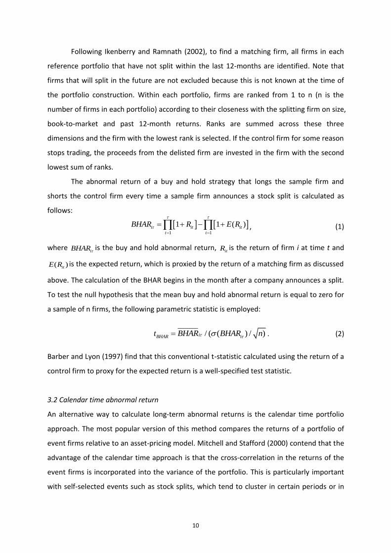
The abnormal return of a buy and hold strategy that longs the sample firm and
shorts the control firm every time a sample firm announces a stock split is calculated as
follows:
, (1)
where iBHAR
is the buy and hold abnormal return, itR is the return of firm i at time t and
( )itE R is the expected return, which is proxied by the return of a matching firm as discussed
above. The calculation of the BHAR begins in the month after a company announces a split.
To test the null hypothesis that the mean buy and hold abnormal return is equal to zero for
a sample of n firms, the following parametric statistic is employed:
/ ( ( ) / )iBHAR it BHAR BHAR n . (2)
Barber and Lyon (1997) find that this conventional t-statistic calculated using the return of a
control firm to proxy for the expected return is a well-specified test statistic.
3.2 Calendar time abnormal return
An alternative way to calculate long-term abnormal returns is the calendar time portfolio
approach. The most popular version of this method compares the returns of a portfolio of
event firms relative to an asset-pricing model. Mitchell and Stafford (2000) contend that the
advantage of the calendar time approach is that the cross-correlation in the returns of the
event firms is incorporated into the variance of the portfolio. This is particularly important
with self-selected events such as stock splits, which tend to cluster in certain periods or in
11
specific industries. To implement the calendar time approach, equal-weighted portfolios of
all firms that announce a split within the last year are formed. The portfolios are rebalanced
monthly to remove firms that reach the end of their one-year period and add companies
that have just split their shares. Following Mitchell and Stafford (2000), months where the
number of firms in the split portfolio is less than 10 are excluded from the analysis. This is to
mitigate heteroskedasticity arising from changes in the number of firms in the split portfolio.
As splitting firms typically have a run-up in price before they split, momentum may
relate to subsequent returns. Therefore, the Carhart (1997) model, which accounts for
momentum is used instead of the Fama-French (1993) model when calculating abnormal
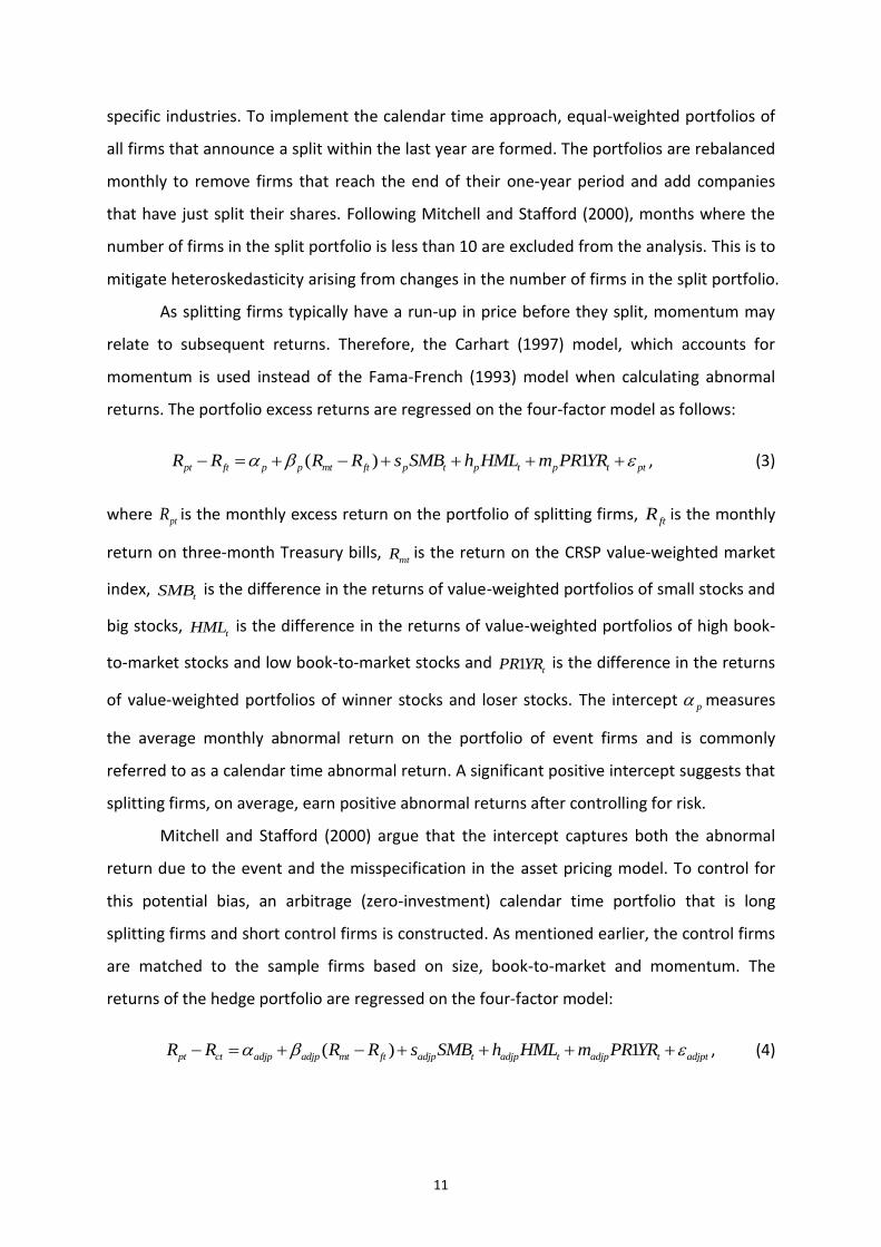
returns. The portfolio excess returns are regressed on the four-factor model as follows:
( ) 1pt ft p p mt ft p t p t p t ptR R R R s SMB h HML m PR YR , (3)
where ptR is the monthly excess return on the portfolio of splitting firms, ftR is the monthly
return on three-month Treasury bills, mtR is the return on the CRSP value-weighted market
index, tSMB is the difference in the returns of value-weighted portfolios of small stocks and
big stocks, tHML is the difference in the returns of value-weighted portfolios of high book-
to-market stocks and low book-to-market stocks and 1 tPR YR is the difference in the returns
of value-weighted portfolios of winner stocks and loser stocks. The intercept p measures
the average monthly abnormal return on the portfolio of event firms and is commonly
referred to as a calendar time abnormal return. A significant positive intercept suggests that
splitting firms, on average, earn positive abnormal returns after controlling for risk.
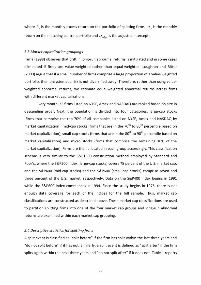
Mitchell and Stafford (2000) argue that the intercept captures both the abnormal
return due to the event and the misspecification in the asset pricing model. To control for
this potential bias, an arbitrage (zero-investment) calendar time portfolio that is long
splitting firms and short control firms is constructed. As mentioned earlier, the control firms
are matched to the sample firms based on size, book-to-market and momentum. The
returns of the hedge portfolio are regressed on the four-factor model:
( ) 1pt ct adjp adjp mt ft adjp t adjp t adjp t adjptR R R R s SMB h HML m PR YR , (4)
12
where ptR is the monthly excess return on the portfolio of splitting firms, ctR is the monthly
return on the matching control portfolio and adjp is the adjusted intercept.
3.3 Market capitalization groupings
Fama (1998) observes that drift in long-run abnormal returns is mitigated and in some cases
eliminated if firms are value-weighted rather than equal-weighted. Loughran and Ritter
(2000) argue that if a small number of firms comprise a large proportion of a value-weighted
portfolio, then unsystematic risk is not diversified away. Therefore, rather than using value-
weighted abnormal returns, we estimate equal-weighted abnormal returns across firms
with different market capitalizations.
Every month, all firms listed on NYSE, Amex and NASDAQ are ranked based on size in
descending order. Next, the population is divided into four categories: large-cap stocks
(firms that comprise the top 70% of all companies listed on NYSE, Amex and NASDAQ by
market capitalization), mid-cap stocks (firms that are in the 70th to 80th percentile based on
market capitalization), small-cap stocks (firms that are in the 80th to 90th percentile based on
market capitalization) and micro stocks (firms that comprise the remaining 10% of the
market capitalization). Firms are then allocated in each group accordingly. This classification
scheme is very similar to the S&P1500 construction method employed by Standard and
Poor’s, where the S&P500 index (large-cap stocks) covers 75 percent of the U.S. market cap,
and the S&P400 (mid-cap stocks) and the S&P600 (small-cap stocks) comprise seven and
three percent of the U.S. market, respectively. Data on the S&P400 index begins in 1991
while the S&P600 index commences in 1994. Since the study begins in 1975, there is not
enough data coverage for each of the indices for the full sample. Thus, market cap
classifications are constructed as described above. These market cap classifications are used
to partition splitting firms into one of the four market cap groups and long-run abnormal
returns are examined within each market cap grouping.
3.4 Descriptive statistics for splitting firms
A split event is classified as “split before” if the firm has split within the last three years and
“do not split before” if it has not. Similarly, a split event is defined as “split after” if the firm
splits again within the next three years and “do not split after” if it does not. Table 1 reports
13
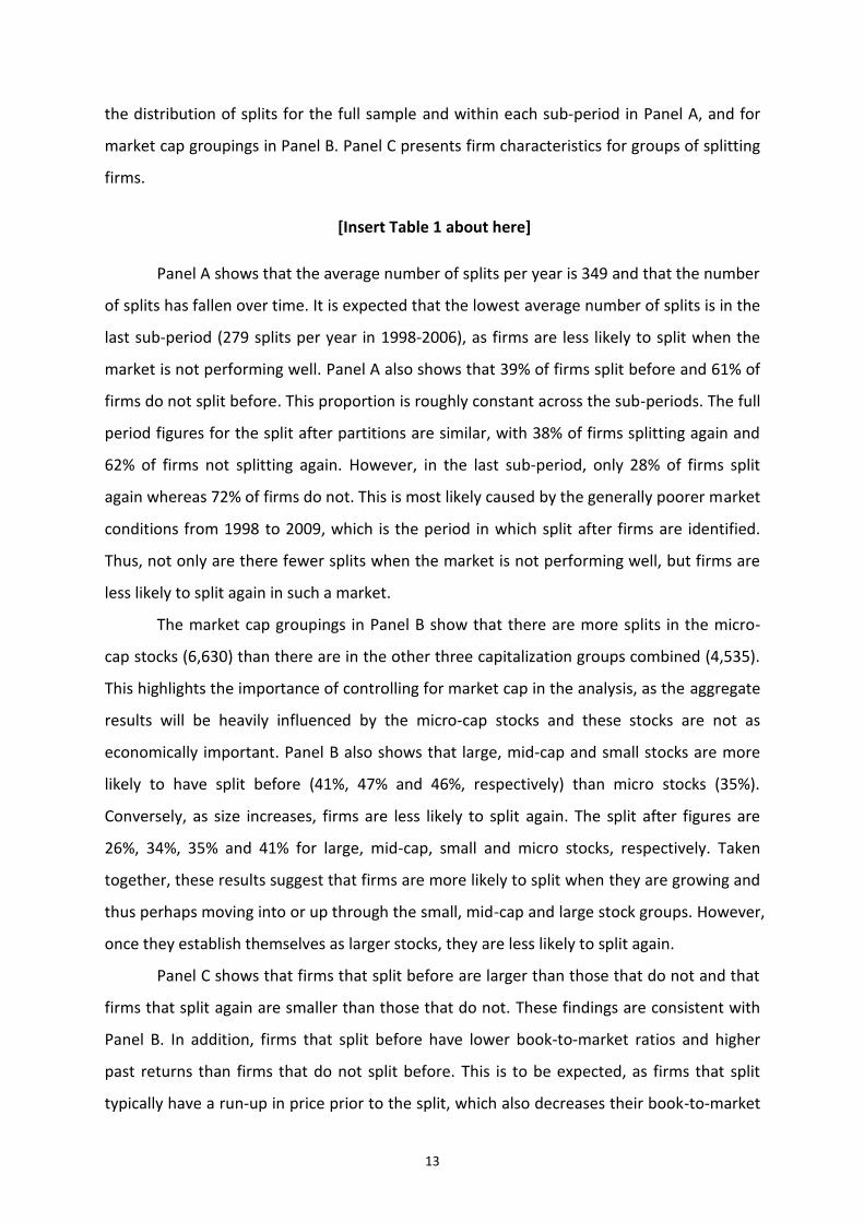
the distribution of splits for the full sample and within each sub-period in Panel A, and for
market cap groupings in Panel B. Panel C presents firm characteristics for groups of splitting
firms.
[Insert Table 1 about here]
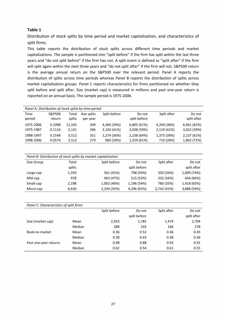
Panel A shows that the average number of splits per year is 349 and that the number
of splits has fallen over time. It is expected that the lowest average number of splits is in the
last sub-period (279 splits per year in 1998-2006), as firms are less likely to split when the
market is not performing well. Panel A also shows that 39% of firms split before and 61% of
firms do not split before. This proportion is roughly constant across the sub-periods. The full
period figures for the split after partitions are similar, with 38% of firms splitting again and
62% of firms not splitting again. However, in the last sub-period, only 28% of firms split
again whereas 72% of firms do not. This is most likely caused by the generally poorer market
conditions from 1998 to 2009, which is the period in which split after firms are identified.
Thus, not only are there fewer splits when the market is not performing well, but firms are
less likely to split again in such a market.
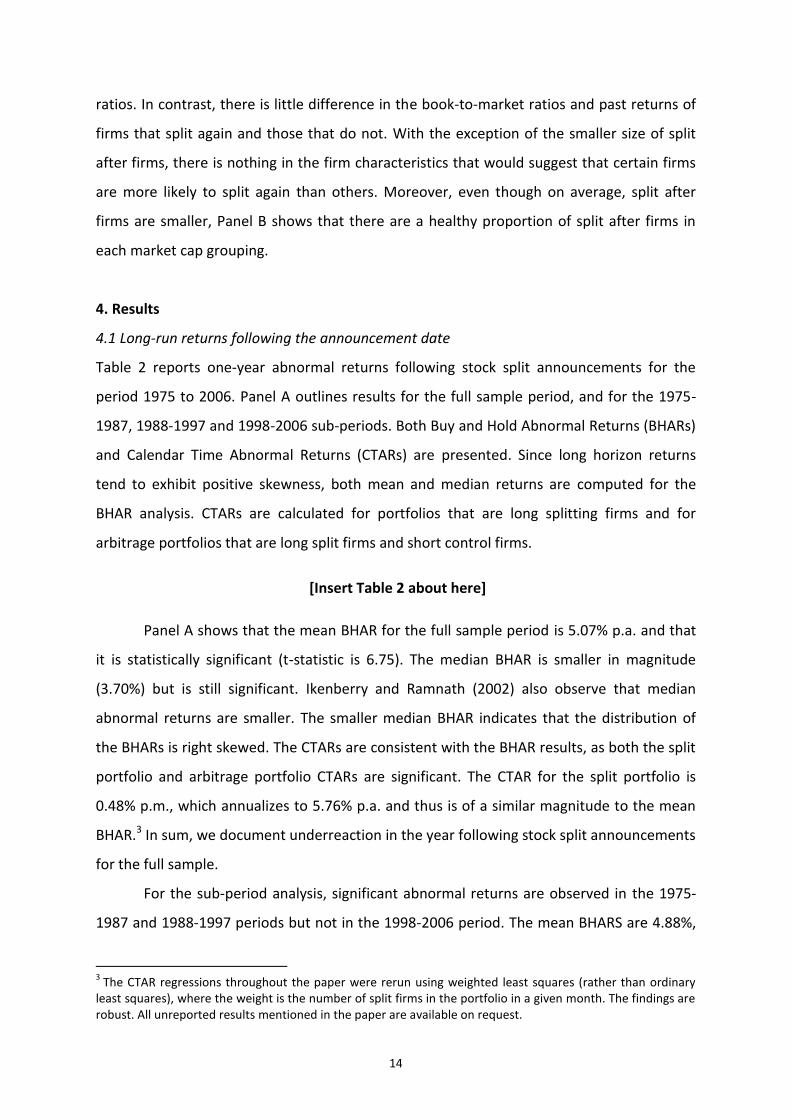
The market cap groupings in Panel B show that there are more splits in the micro-
cap stocks (6,630) than there are in the other three capitalization groups combined (4,535).
This highlights the importance of controlling for market cap in the analysis, as the aggregate
results will be heavily influenced by the micro-cap stocks and these stocks are not as
economically important. Panel B also shows that large, mid-cap and small stocks are more
likely to have split before (41%, 47% and 46%, respectively) than micro stocks (35%).
Conversely, as size increases, firms are less likely to split again. The split after figures are
26%, 34%, 35% and 41% for large, mid-cap, small and micro stocks, respectively. Taken
together, these results suggest that firms are more likely to split when they are growing and
thus perhaps moving into or up through the small, mid-cap and large stock groups. However,
once they establish themselves as larger stocks, they are less likely to split again.
Panel C shows that firms that split before are larger than those that do not and that
firms that split again are smaller than those that do not. These findings are consistent with
Panel B. In addition, firms that split before have lower book-to-market ratios and higher
past returns than firms that do not split before. This is to be expected, as firms that split
typically have a run-up in price prior to the split, which also decreases their book-to-market
14
ratios. In contrast, there is little difference in the book-to-market ratios and past returns of
firms that split again and those that do not. With the exception of the smaller size of split
after firms, there is nothing in the firm characteristics that would suggest that certain firms
are more likely to split again than others. Moreover, even though on average, split after
firms are smaller, Panel B shows that there are a healthy proportion of split after firms in
each market cap grouping.
4. Results
4.1 Long-run returns following the announcement date
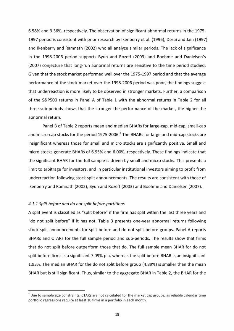
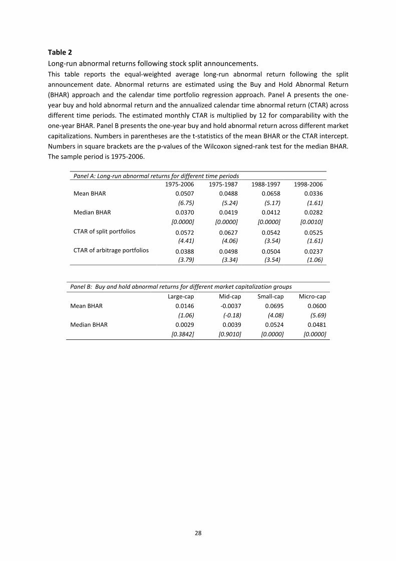
Table 2 reports one-year abnormal returns following stock split announcements for the
period 1975 to 2006. Panel A outlines results for the full sample period, and for the 1975-
1987, 1988-1997 and 1998-2006 sub-periods. Both Buy and Hold Abnormal Returns (BHARs)
and Calendar Time Abnormal Returns (CTARs) are presented. Since long horizon returns
tend to exhibit positive skewness, both mean and median returns are computed for the
BHAR analysis. CTARs are calculated for portfolios that are long splitting firms and for
arbitrage portfolios that are long split firms and short control firms.
[Insert Table 2 about here]
Panel A shows that the mean BHAR for the full sample period is 5.07% p.a. and that
it is statistically significant (t-statistic is 6.75). The median BHAR is smaller in magnitude
(3.70%) but is still significant. Ikenberry and Ramnath (2002) also observe that median
abnormal returns are smaller. The smaller median BHAR indicates that the distribution of
the BHARs is right skewed. The CTARs are consistent with the BHAR results, as both the split
portfolio and arbitrage portfolio CTARs are significant. The CTAR for the split portfolio is
0.48% p.m., which annualizes to 5.76% p.a. and thus is of a similar magnitude to the mean
BHAR.3 In sum, we document underreaction in the year following stock split announcements
for the full sample.
For the sub-period analysis, significant abnormal returns are observed in the 1975-
1987 and 1988-1997 periods but not in the 1998-2006 period. The mean BHARS are 4.88%,
3 The CTAR regressions throughout the paper were rerun using weighted least squares (rather than ordinary
least squares), where the weight is the number of split firms in the portfolio in a given month. The findings are robust. All unreported results mentioned in the paper are available on request.
15
6.58% and 3.36%, respectively. The observation of significant abnormal returns in the 1975-
1997 period is consistent with prior research by Ikenberry et al. (1996), Desai and Jain (1997)
and Ikenberry and Ramnath (2002) who all analyze similar periods. The lack of significance
in the 1998-2006 period supports Byun and Rozeff (2003) and Boehme and Danielsen’s
(2007) conjecture that long-run abnormal returns are sensitive to the time period studied.
Given that the stock market performed well over the 1975-1997 period and that the average
performance of the stock market over the 1998-2006 period was poor, the findings suggest
that underreaction is more likely to be observed in stronger markets. Further, a comparison
of the S&P500 returns in Panel A of Table 1 with the abnormal returns in Table 2 for all
three sub-periods shows that the stronger the performance of the market, the higher the
abnormal return.
Panel B of Table 2 reports mean and median BHARs for large-cap, mid-cap, small-cap
and micro-cap stocks for the period 1975-2006.4 The BHARs for large and mid-cap stocks are
insignificant whereas those for small and micro stocks are significantly positive. Small and
micro stocks generate BHARs of 6.95% and 6.00%, respectively. These findings indicate that
the significant BHAR for the full sample is driven by small and micro stocks. This presents a
limit to arbitrage for investors, and in particular institutional investors aiming to profit from
underreaction following stock split announcements. The results are consistent with those of
Ikenberry and Ramnath (2002), Byun and Rozeff (2003) and Boehme and Danielsen (2007).
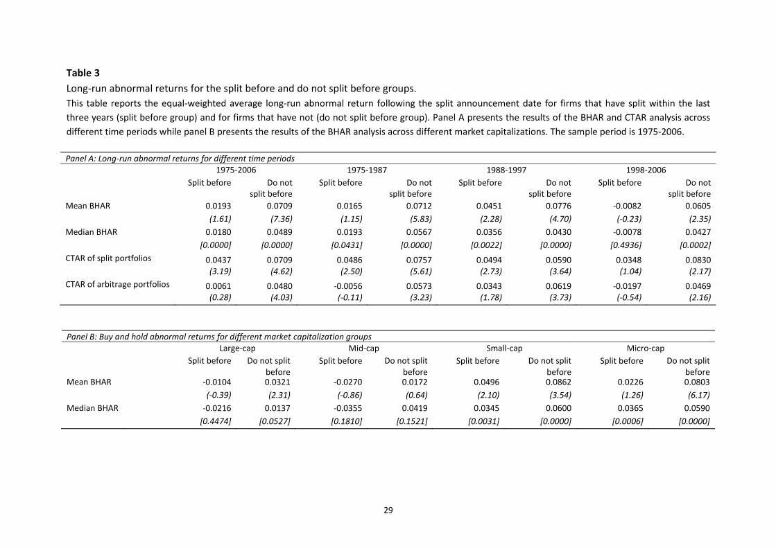
4.1.1 Split before and do not split before partitions
A split event is classified as “split before” if the firm has split within the last three years and
“do not split before” if it has not. Table 3 presents one-year abnormal returns following
stock split announcements for split before and do not split before groups. Panel A reports
BHARs and CTARs for the full sample period and sub-periods. The results show that firms
that do not split before outperform those that do. The full sample mean BHAR for do not
split before firms is a significant 7.09% p.a. whereas the split before BHAR is an insignificant
1.93%. The median BHAR for the do not split before group (4.89%) is smaller than the mean
BHAR but is still significant. Thus, similar to the aggregate BHAR in Table 2, the BHAR for the
4 Due to sample size constraints, CTARs are not calculated for the market cap groups, as reliable calendar time
portfolio regressions require at least 10 firms in a portfolio in each month.

16
do not split before group is right skewed. Although the mean BHAR for the split before
group is not significant, the median BHAR and the CTAR for the split portfolio are.
In sub-period analyses, the mean BHAR for the do not split before group is always
significant and always larger than for the split before group. Further, whereas the aggregate
BHAR was not significant in the 1998-2006 period, the do not split before BHAR is a healthy
6.05% p.a. in this period. Contrastingly, the mean BHAR for the split before group is only
significant in the 1988-1997 period. Panel B presents BHARs for the market cap groupings.
The split before mean BHAR is significant in small stocks but insignificant in large, mid-cap
and micro stocks. Conversely, the do not split before mean BHAR is significant in all bar the
mid-cap stocks.
[Insert Table 3 about here]
Overall, firms that have not split within the past three years perform much better
than firms that have in the year after split announcements. This is similar to a result by
Huang et al. (2008) who find that infrequent splitters perform better than frequent splitters
in the year after a split. Thus, it appears that the market is underreacting to the inherently
stronger signal in a firm splitting for the first time in at least three years. For investors
trading on stock split announcements, the findings suggest that they should focus on firms
that split for the first time in a number of years.
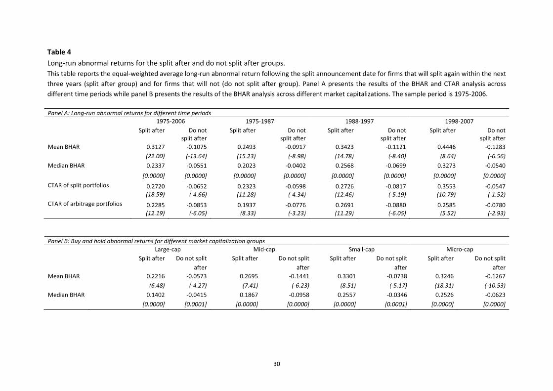
4.1.2 Split after and do not split after partitions
A split event is classified as “split after” if the firm splits again within the next three years
and “do not split after” if it does not. The one-year abnormal returns for both groups are
presented in Table 4. For the split after group, the mean BHAR for the full sample is 31.27%
p.a. and is highly significant. In contrast, the mean BHAR for the do not split after group is -
10.75%, which is also highly significant. The corresponding median BHARs are 23.37% and -
5.51% for the split after and do not split after groups, respectively. The median BHARs
indicate a strong right (left) skew in the BHARs for the split after (do not split after) samples.
Nevertheless, the median BHARs are still large in magnitude and highly significant. The CTAR
findings are consistent with those on the BHARs.
[Insert Table 4 about here]
17
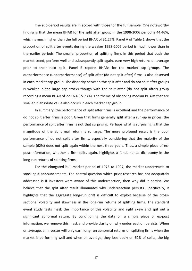
The sub-period results are in accord with those for the full sample. One noteworthy
finding is that the mean BHAR for the split after group in the 1998-2006 period is 44.46%,
which is much higher than the full period BHAR of 31.27%. Panel A of Table 1 shows that the
proportion of split after events during the weaker 1998-2006 period is much lower than in
the earlier periods. The smaller proportion of splitting firms in this period that buck the
market trend, perform well and subsequently split again, earn very high returns on average
prior to their next split. Panel B reports BHARs for the market cap groups. The
outperformance (underperformance) of split after (do not split after) firms is also observed
in each market cap group. The disparity between the split after and do not split after groups
is weaker in the large cap stocks though with the split after (do not split after) group
recording a mean BHAR of 22.16% (-5.73%). The theme of observing median BHARs that are
smaller in absolute value also occurs in each market cap group.
In summary, the performance of split after firms is excellent and the performance of
do not split after firms is poor. Given that firms generally split after a run-up in prices, the
performance of split after firms is not that surprising. Perhaps what is surprising is that the
magnitude of the abnormal return is so large. The more profound result is the poor
performance of do not split after firms, especially considering that the majority of the
sample (62%) does not split again within the next three years. Thus, a simple piece of ex-
post information, whether a firm splits again, highlights a fundamental dichotomy in the
long-run returns of splitting firms.
For the elongated bull market period of 1975 to 1997, the market underreacts to
stock split announcements. The central question which prior research has not adequately
addressed is if investors were aware of this underreaction, then why did it persist. We
believe that the split after result illuminates why underreaction persists. Specifically, it
highlights that the aggregate long-run drift is difficult to exploit because of the cross-
sectional volatility and skewness in the long-run returns of splitting firms. The standard
event study tests mask the importance of this volatility and right skew and spit out a
significant abnormal return. By conditioning the data on a simple piece of ex-post
information, we remove this mask and provide clarity on why underreaction persists. When
on average, an investor will only earn long-run abnormal returns on splitting firms when the
market is performing well and when on average, they lose badly on 62% of splits, the big
18
wins they make on the other 38% of splits might not be enough to compensate them for the
risk they bear.
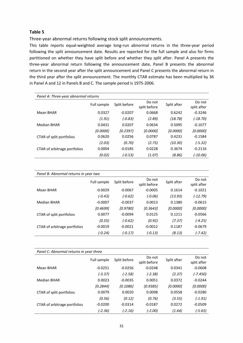
4.2 Three-year returns following the announcement date
Up to this point, abnormal returns are only examined in the year following split
announcements. Given that we look forward three years to identify whether firms split
again, it is pertinent to analyze abnormal returns over a three-year horizon. Table 5 outlines
these results. Panel A reports three-year abnormal returns whereas Panels B and C present
abnormal returns in years two and three, respectively.
[Insert Table 5 about here]
Panel A shows that the three-year mean BHAR for the full sample is 3.27% (t-statistic
of 1.91). This is smaller than the one-year BHAR in Table 2, which is 5.07%. Thus, there is
reversion in returns after the first year. Panels B and C show that the reversion mainly
occurs in the third year where a significant mean BHAR of -2.51% is observed. The median
BHAR in Panel A is 4.31% and thus is higher than the mean. This indicates that over three
years, the BHARs are left skewed. This is in contrast to the one-year BHARs, which are right
skewed. Panel A shows that the CTAR of the split portfolio is significantly positive whereas
the CTAR of the arbitrage portfolio is insignificant, which suggests that the abnormal return
over three years is not economically large, as its significance is conditional on the method
employed. The reversion in returns between the first and third years is consistent with the
findings of Boehme and Danielsen (2007) and Hwang et al. (2008).
The findings for the split before and do not split before samples also demonstrate a
reversion in returns. Panel A shows that the split before mean BHAR falls from 1.65% over
one year (Table 3) to -2.07% over three years. Similarly, the do not split before BHAR falls
from 7.12% over one year to 6.68% over three years but remains significant. As with the full
sample, Panel C shows that the reversion mainly occurs in the third year. For the split after
and do not split after samples and in contrast to the full sample and the split before groups,
there is continuation in returns. In Panel A, the mean BHAR for the split after group is a huge
62.42% over three years. Further, Panels B and C show that the abnormal returns in years
two and three are significantly positive. As firms are more likely to split after a run-up in
prices and as we identify split after firms as those that split again within the next three years,
19
the continuation in returns for the split after sample is not surprising. The three-year mean
BHAR for the do not split after group in Panel A is -32.46%. This is much larger in absolute
value than the one-year BHAR in Table 4, which is -10.75%. This is because do not split after
firms record significantly negative BHARs in years two and three, which amount to -10.21%
and -6.08%, respectively. Therefore, the poor performance of firms that do not split after is
not confined to the year after split announcements but extends out to three years. This
reinforces our conjecture that trading on stock splits is a very risky proposition. If firms do
not split again, then on average, investors long these firms will suffer considerable losses for
at least three years.
4.3 Long-run returns following the effective date
Byun and Rozeff (2003) and Boehme and Danielsen (2007) find that long-run abnormal
returns shrink considerably when calculated following the effective date of the split rather
than the announcement date. They contend that firms do not exhibit post-split abnormal
returns and that the post-announcement drift only lasts a short duration. We argue that if
investors believe that long-run abnormal returns can be earned from trading on stocks splits,
then they would trade as soon as the information becomes public, that is, following the
announcement date. Thus, the majority of our analysis is conducted after the
announcement date. However, in response to the findings of Byun and Rozeff (2003) and
Boehme and Danielsen (2007), we also calculate long-run abnormal returns following the
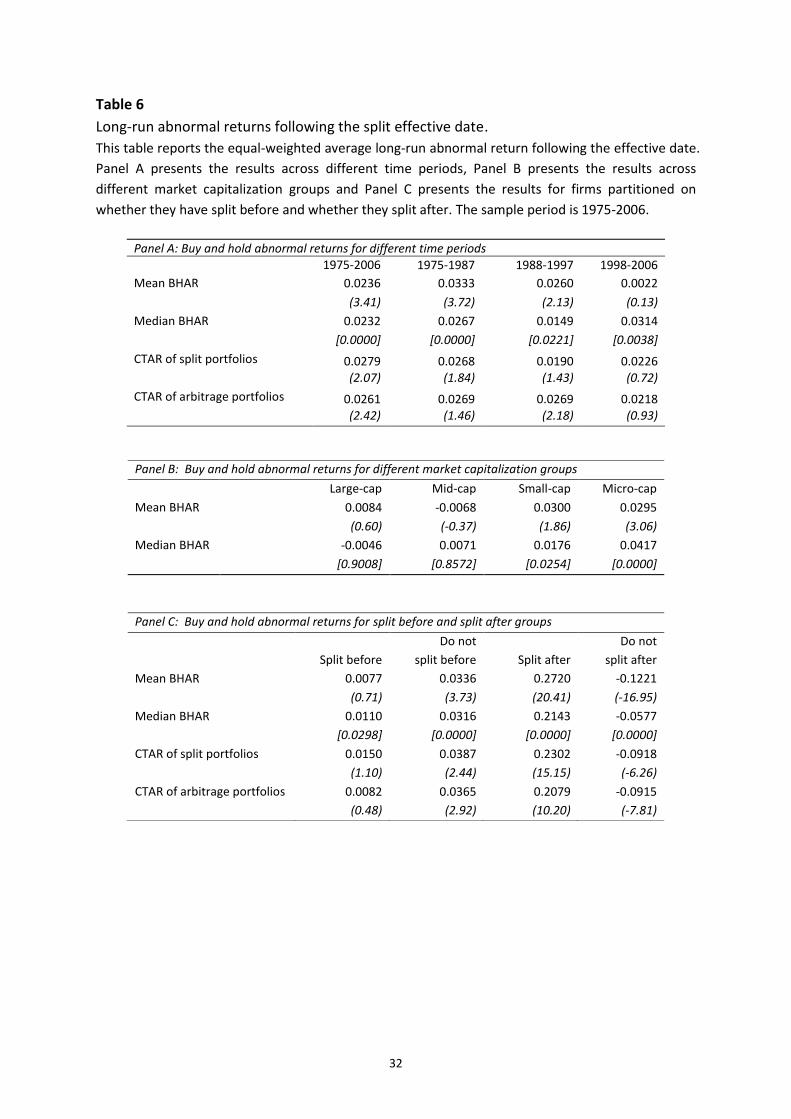
effective date. Table 6 presents the results.
[Insert Table 6 about here]
Panel A shows that the full sample mean BHAR is 2.36% p.a. Although significant, it is
smaller than the 5.07% BHAR in Table 2 calculated following the announcement date. In an
untabulated result, it is observed that the average (median) number of days between the
announcement and effective date is 40 (35). Therefore, consistent with Boehme and
Danielsen (2007), we see that abnormal returns are smaller after the effective date and that
a considerable portion of the long-run abnormal return following the split announcement is
concentrated in the short period between the announcement and effective dates. The
BHARs in the 1975-1987 and 1988-1997 periods are also significant but as expected, they
are smaller than the corresponding announcement day BHARs in Table 2. The CTARs in
20
these two sub-periods are mostly insignificant though, which suggests that the abnormal
returns are not economically meaningful. The median BHARs over the full sample period
and in the 1975-1987 and 1988-1997 sub-periods are much closer to the means than they
were in Table 2, which indicates that there is less of a right skew in the BHARs after the
effective date compared to the announcement date. In the 1998-2006 period and consistent
with the announcement date results, the mean BHAR and both CTAR estimates are
insignificant. In contrast, the median BHAR is significant, a result that was also observed in
Table 2. Thus, although on balance, we conclude that there are no abnormal returns in the
1998-2006 period, the median BHARs suggest that there is weak evidence of positive
abnormal returns in this period. The market cap results in Panel B and the results of the split
before and split after partitions in Panel C follow the same theme as the announcement
date results, the only difference is the abnormal returns are smaller. In summary, the
patterns in the abnormal returns after the effective date are consistent with those after the
announcement date and in accord with prior research, the key difference is the abnormal
returns are smaller.
4.4 Short-run returns around the announcement date
Having examined long-run returns one year after the announcement and effective dates,
and three years after the announcement date, short-run returns in the three days around
the split announcement are now analyzed. Beginning with Grinblatt et al. (1984), numerous
studies have documented positive returns when splits are announced. Of particular
importance to this study and what has not been considered previously are the short-run
returns of the split before and split after partitions. As we observe that do not split before
firms outperform split before firms and that split after firms considerably outperform do not
split after firms, an analysis of the short-run returns of these groups will allow us to
ascertain whether investors have the ability to identify splitting firms that will subsequently
perform well.
The market model is used to calculate short-run abnormal returns where the model
parameters are estimated over the period [-250, -46] trading days prior to the split
announcement. The abnormal return is the disturbance term from the market model. The
return of the CRSP equally-weighted index is used to proxy for the return of the market
portfolio, as Brown and Warner (1980) find that tests using the return of a value-weighted

21
index are severely misspecified. The abnormal returns over the [-1, +1] period where day 0
is the announcement date are summed to form the cumulative abnormal return (CAR). A
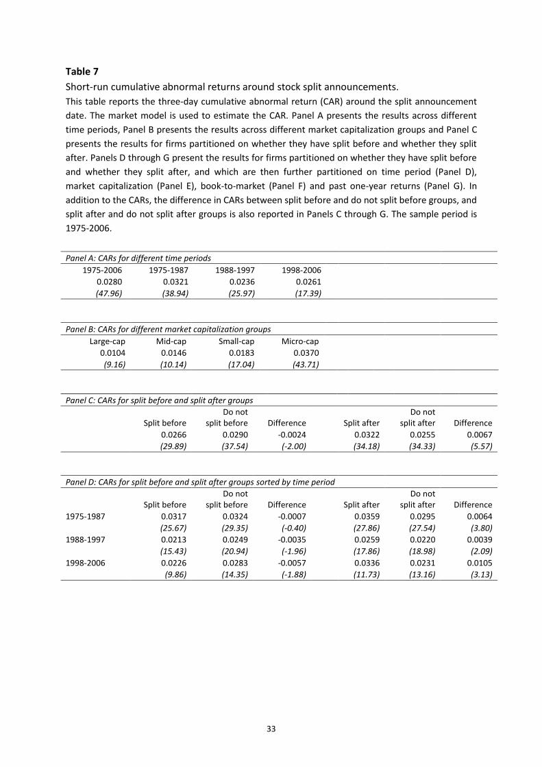
standard parametric t-statistic is employed to infer its significance. Table 7 presents the
findings of the short-run CAR analysis.5
[Insert Table 7 about here]
As expected and consistent with prior research, the CAR around the announcement
date is positive and highly significant. The full sample CAR in Panel A is 2.8% over three days.
The CARs over all sub-periods (Panel A) and all market cap groups (Panel B) are also
significant. Further, in accord with Ikenberry et al. (1996), it is observed that CARs decrease
as firms get larger. Panel C shows that the CARs are significantly positive for the split before,
do not split before, split after and do not split after groups. Moreover, do not split before
firms earn a significantly higher CAR than split before firms. This is similar to a result
documented by Huang et al. (2008) on infrequent and frequent splitters. Further, split after
firms earn a significantly higher CAR than do not split after firms. Recall that over one to
three year periods, do not split before firms outperform split before firms and split after
firms considerably outperform do not split after firms. Given this, the findings on the split
before and split after groups are very interesting because they suggest that at the time of
the split announcement, investors are displaying a capacity to determine which firms will
subsequently perform better. These results warrant further investigation.
Panel D shows that the difference in CARs between the split before and do not split
before groups is insignificant in the 1975-1987 period, significant in the 1988-1997 period
and marginally significant in the 1998-2006 period. In Panels E and F, the CAR difference
between the split before and do not split before groups is insignificant across all market cap
and all book-to-market partitions. Finally, only the second lowest past return quartile in
Panel G has a significant difference in CARs. Therefore, the significantly higher CAR observed
in Panel C for the do not split before group compared to the split before group is not robust
5 A number of unreported robustness tests are also conducted. First, in addition to the market model
estimations, CARs are also estimated using the constant mean return model. Second, t-statistics for zero standardized CARs are calculated following Patell (1976) and Boehmer, Masumeci and Poulsen (1991). Third, as a complement to the t-test, the Mann-Whitney-Wilcoxon test is used to evaluate the significance of the CAR differences. The findings are robust.
22
to sub-period analyses and to market cap, book-to-market and past one-year return
partitions.
In contrast, Panels D to G show that the significantly higher CAR for split after firms
relative to do not split after firms is generally robust. It is significant across all sub-periods in
Panel D and all market cap groups except for mid-cap stocks in Panel E. The CAR difference
between large-cap stocks is 1.03% and it is more than double the CAR difference in the
other three capitalization groups. This suggests that investors are best able to identify which
splitting firms will subsequently perform well when firms are large. It may also be a reason
why in Table 4, the return difference between split after and do not split after firms in the
year following splits is lowest for the large-cap stocks. Panel F shows that the difference in
CARs is only significant for the second highest and highest book-to-market groups. Further,
the CAR difference increases as book-to-market increases. In Panel G, the difference in CARs
is significant in all but the highest past one-year return quartile. Similar to Panel F, there is
also a clear pattern in the CAR difference, which falls as past returns increase. All else
constant, firms with higher book-to-market ratios or lower past returns are less likely to split.
Therefore, it appears that at that time of the split announcement, investors are best able to
identify whether firms will subsequently perform better in firms that ex-ante, were least
likely to split.
In summary, the short-run CAR analysis in Table 7 has provided some important
insights on investor behavior when firms split. Most interestingly, there is evidence that at
the time of the split announcement, investors are demonstrating some proficiency in
identifying which firms will subsequently perform better and investing accordingly. However,
as the CARs on the do not split after groups are always significantly positive, this indicates
that investors are not identifying that on average, the firms in these groups subsequently
perform poorly. Moreover, the significantly positive CARs support our contention that for
the do not split after group, the market overreacts to the split announcement. Finally, and in
aggregate, as there is long-run positive drift observed following splits, the average price
reaction when splits are announced is not complete.
*****No discussion yet of Tables 8 to 12*****
23
6. Conclusion
Long-run return performance following stock splits has been debated by researchers for
over 40 years. The weight of evidence in this paper and others indicates that at least for the
period 1975 to 1997, the market underreacts to split announcements. The common claim by
those arguing against underreaction is that it is specific to certain eras. The absence of drift
observed in this study during the weaker market period from 1998 to 2006 supports this
claim. Nevertheless, given that underreaction has been observed for over 20 years and that
there is evidence, albeit weaker evidence of drift in other periods, the time period specific
argument is not compelling. Behavioral models have been proposed to explain why
underreaction following corporate actions may occur. The drawback of these models is that
do not explain why underreaction persists over the long term. It seems unreasonable to
assume that for more than 20 years, psychological biases by investors were constraining
learning and thus perpetuating the underreaction.
When splits are announced, the market reacts positively. In the long-run, there will
obviously be firms who perform well and others who do not. Our findings show that at the
time of the split announcement, investors are displaying an ability to determine which firms
subsequently perform better. Despite this, they still react positively to splitting firms that
subsequently perform poorly. The challenge for investors is to infer the information in the
split signal and correctly impound this into the price of splitting stocks so that in aggregate,
there is no post-split drift observed. Our findings show that on average, investors are
correctly impounding the signal in splits when the future performance of the market is weak
but that they are underreacting when the future performance of the market is strong.
The demarcation of firms into those that split again and those that do not is an
instrument we use to identify the minority of firms that perform very well and the majority
who do not perform well post-split. This demarcation allows us to highlight a fundamental
dichotomy in the subsequent performance of splitting firms, which provides insight on why
on average, investors underreact when the future performance of the market is strong. In a
weaker market, the very good performance of the minority is cancelled out by the poor
performance of the majority. In a strong market, the very good performance of a larger
minority outweighs the poor performance of a smaller majority, which results in aggregate
underreaction. Thus, when the future performance of the market is strong, investors are
underestimating the degree of right skew in the long-run return distribution of splitting

24
firms and the extent to which firms in the right tail of this distribution will outperform. It is
possible that the underreaction observed is driven by behavioral biases but we do not
believe that this is the case. It is more likely that it is driven by rational errors in information
processing by investors on the future performance of the market and the performance of
splitting firms in such a market. If the underreaction documented is caused by rational
errors by investors, then this would be consistent with theoretical modeling by Brav and
Heaton (2002).
The presence of underreaction following splits for more than 20 years suggests that
informed investors were most likely aware of this underreaction. If so, why did they not
arbitrage it away? The first key limit to arbitrage is that abnormal returns are concentrated
in small and micro stocks. Second, the volatility and right skew in the long-run returns of
splitting firms means that investors would have to trade on the vast majority of split
announcements to maximize their chance of earning an abnormal return. Third,
underreaction is conditional on the strong future performance of the market and thus, to
exploit the underreaction, investors would have to able to forecast the long-run
performance of the market. In conclusion, trading on stock splits is not an easy means by
which investors can earn long-run abnormal returns, even when the market underreacts to
split announcements.
25
References
Angel, J.J., 1997. Tick size, share prices and stock splits. Journal of Finance 52, 655-681. Baker, H.K., Gallagher, P.L., 1980. Management’s view of stock splits. Financial Management
9, 73-77. Barber, B. M., Lyon, J. D., 1997. Detecting long run abnormal stock returns: the empirical
power and specification of test statistics. Journal of Financial Economics 43, 341-372. Barberis, N., Shleifer, A., Vishny, R., 1998. A model of investor sentiment. Journal of
Financial Economics 49, 307-343 Brav, A., Heaton, J.B., 2002. Competing theories of financial anomalies. Review of Financial
Studies 15, 575-606. Boehme, R. D., Danielsen, B. R., 2007. Stock split post-announcement returns: underreaction
or market friction. Financial Review 42, 485-506. Boehmer, E., Masumeci, J., Poulsen, A., 1991. Event study methodology under conditions of
event induced variance. Journal of Financial Economics 30, 1-48. Brennan, M.J., Copeland, T.E., 1988. Stock splits, stock prices, and transaction costs. Journal
of Financial Economics 22, 83-101. Brennan, M.J., Hughes, P.J., 1991. Stock prices and the supply of information. Journal of
Finance 46, 1665-1691. Brown, S.J., Warner, J.B., 1980. Measuring security price performance. Journal of Financial
Economics 8, 205-258. Byun, J., Rozeff, M. S., 2003. Long-run performance after stock splits: 1927 to 1996. Journal
of Finance 58, 1063-1085. Carhart, M., 1997. On persistence in mutual fund performance. Journal of Finance 52, 57-82. Conrad, J., Kaul, G., 1993. Long-term market overreaction or biases in computed returns?
Journal of Finance 48, 39-63. Daniel, K., Hirshleifer, D., Subrahmanyam, A., 1998. Investor psychology and security market
under- and overreactions. Journal of Finance 53, 1839-1885. Desai, H., Jain, P.C., 1997. Long run common stock returns following stock splits and reverse
splits. Journal of Business 70, 409-433. Easley, D., O’Hara, M., Saar, G., 2001. How stock splits affect trading: A microstructure
approach. Journal of Financial and Quantitative Analysis 36, 25-51. Fama, E.F., 1998. Market efficiency, long term returns and behavioral finance. Journal of
Financial Economics 49, 283-306. Fama, E.F., Fisher, L., Jensen, M., Roll, R., 1969. The adjustment of stock prices to new
information. International Economic Review 10, 1-21. Fama, E.F, French, K.R., 1993. Common risk factors in the returns on stocks and bonds.
Journal of Financial Economics 33, 3-56. Greenwood, R., 2009. Trading restrictions and stock prices. Review of Financial Studies 22,
509-539. Grinblatt, M.S., Masulis, R.W., Titman, S., 1984. The valuation effects of stock splits and
stock dividends. Journal of Financial Economics 13, 461-490. Huang, G.C., Liano, K., Manakyan, H., Pan, M.S., 2008. The information content of multiple
stock splits. Financial Review 43, 543-567. Hwang, S., Keswani, A., Shackleton, M., 2008. Surprise versus anticipated information
announcements: are prices affected differently? An investigation in the context of stock splits. Journal of Banking and Finance 32, 643–653.
26
Ikenberry, D. L., Ramnath, S., 2002. Underreaction to self selected news events: the case of stock splits. Review of Financial Studies 15, 489-526.
Ikenberry, D. L., Rankine, G., Stice, E. K., 1996. What do stock splits really signal? Journal of Financial and Quantitative Analysis 31, 357-375.
Lakonishok, J., Lev, B., 1987. Stock splits and stock dividends: why, who and when. Journal of Finance 42, 913-932.
Lamoureux, C.G., Poon, P., 1987. The market reaction to stock splits. Journal of Finance 42, 1347-1370.
Lin, J.C., Singh, A.J., Yu, W., 2009. Stock splits, trading continuity, and the cost of equity capital. Journal of Financial Economics 93, 474-489.
Loughran, T., Ritter, J. R., 1995. The new issues puzzle. Journal of Finance 50, 23-51. Loughran, T., Ritter, J. R., 2000. Uniformly least powerful tests of market efficiency. Journal
of Financial Economics 55, 361-389. Lyon, J. D., Barber, B. M., Tsai, C. L., 1999. Improved methods for tests of long run abnormal
stock returns. Journal of Finance 54, 165-201. McNichols, M., Dravid, A., 1990. Stock dividends, stock splits and signaling. Journal of
Finance 45, 857-879. Mitchell, M. L., Stafford, E., 2000. Managerial decisions and long term stock price
performance. Journal of Business 73, 287-329. Patell, J., 1976. Corporate forecasts of earnings per share and stock price behaviour:
empirical tests. Journal of Accounting Research 14, 246-276. Pilotte, E., Manuel, T., 1996. The market’s response to recurring events the case of stock
splits. Journal of Financial Economics 41, 111-127. Schultz, P., 2000. Stock splits, tick size, and sponsorship. Journal of Finance 55, 429-450. Spiess, D. K., Affleck-Graves, J., 1995. Underperformance in long-run stock returns following
seasoned equity offerings. Journal of Financial Economics 38, 243-267. Titman, S., 2002. Discussion of “Underreaction to self-selected news events”. Review of
Financial Studies 15, 527-531.
27
Table 1
Distribution of stock splits by time period and market capitalization, and characteristics of
split firms.
This table reports the distribution of stock splits across different time periods and market
capitalizations. The sample is partitioned into “split before” if the firm has split within the last three
years and “do not split before” if the firm has not. A split event is defined as “split after” if the firm
will split again within the next three years and “do not split after” if the firm will not. S&P500 return
is the average annual return on the S&P500 over the relevant period. Panel A reports the
distribution of splits across time periods whereas Panel B reports the distribution of splits across
market capitalization groups. Panel C reports characteristics for firms partitioned on whether they
split before and split after. Size (market cap) is measured in millions and past one-year return is
reported on an annual basis. The sample period is 1975-2006.
Panel B: Distribution of stock splits by market capitalization
Size Group Total
splits
Split before Do not
split before
Split after Do not
split after
Large-cap 1,359 561 (41%) 798 (59%) 350 (26%) 1,009 (74%)
Mid-cap 978 463 (47%) 515 (53%) 332 (34%) 646 (66%)
Small-cap 2,198 1,002 (46%) 1,196 (54%) 780 (35%) 1,418 (65%)
Micro-cap 6,630 2,334 (35%) 4,296 (65%) 2,742 (41%) 3,888 (59%)
Panel C: Characteristics of split firms
Split before Do not
split before
Split after Do not
split after
Size (market cap) Mean 2,953 1,785 1,474 2,704
Median 288 193 166 278
Book-to-market Mean 0.36 0.52 0.46 0.45
Median 0.30 0.43 0.38 0.36
Past one-year returns Mean 0.98 0.88 0.93 0.91
Median 0.62 0.54 0.61 0.55
Panel A: Distribution of stock splits by time period
Time period
S&P500 return
Total splits
Ave splits per year
Split before Do not split before
Split after Do not split after
1975-2006 0.1098 11,165 349 4,360 (39%) 6,805 (61%) 4,204 (38%) 6,961 (62%)
1975-1987 0.1116 5,141 396 2,103 (41%) 3,038 (59%) 2,119 (41%)
3,022 (59%) 1988-1997 0.1548 3,512 351 1,274 (36%) 2,238 (64%) 1,375 (39%) 2,137 (61%)
1998-2006 0.0574 2,512 279 983 (39%) 1,529 (61%) 710 (28%) 1,802 (72%)
28
Table 2
Long-run abnormal returns following stock split announcements.
This table reports the equal-weighted average long-run abnormal return following the split
announcement date. Abnormal returns are estimated using the Buy and Hold Abnormal Return
(BHAR) approach and the calendar time portfolio regression approach. Panel A presents the one-
year buy and hold abnormal return and the annualized calendar time abnormal return (CTAR) across
different time periods. The estimated monthly CTAR is multiplied by 12 for comparability with the
one-year BHAR. Panel B presents the one-year buy and hold abnormal return across different market
capitalizations. Numbers in parentheses are the t-statistics of the mean BHAR or the CTAR intercept.
Numbers in square brackets are the p-values of the Wilcoxon signed-rank test for the median BHAR.
The sample period is 1975-2006.
Panel A: Long-run abnormal returns for different time periods 1975-2006 1975-1987 1988-1997 1998-2006
Mean BHAR 0.0507 0.0488 0.0658 0.0336
(6.75) (5.24) (5.17) (1.61)
Median BHAR 0.0370 0.0419 0.0412 0.0282
[0.0000] [0.0000] [0.0000] [0.0010]
CTAR of split portfolios 0.0572 0.0627 0.0542 0.0525 (4.41) (4.06) (3.54) (1.61)
CTAR of arbitrage portfolios 0.0388 0.0498 0.0504 0.0237 (3.79) (3.34) (3.54) (1.06)
Panel B: Buy and hold abnormal returns for different market capitalization groups
Large-cap Mid-cap Small-cap Micro-cap
Mean BHAR 0.0146 -0.0037 0.0695 0.0600
(1.06) (-0.18) (4.08) (5.69)
Median BHAR 0.0029 0.0039 0.0524 0.0481
[0.3842] [0.9010] [0.0000] [0.0000]
29
Table 3
Long-run abnormal returns for the split before and do not split before groups.
This table reports the equal-weighted average long-run abnormal return following the split announcement date for firms that have split within the last
three years (split before group) and for firms that have not (do not split before group). Panel A presents the results of the BHAR and CTAR analysis across
different time periods while panel B presents the results of the BHAR analysis across different market capitalizations. The sample period is 1975-2006.
Panel A: Long-run abnormal returns for different time periods
1975-2006 1975-1987 1988-1997 1998-2006
Split before Do not split before
Split before Do not split before
Split before Do not split before
Split before Do not split before
Mean BHAR 0.0193 0.0709 0.0165 0.0712 0.0451 0.0776 -0.0082 0.0605
(1.61) (7.36) (1.15) (5.83) (2.28) (4.70) (-0.23) (2.35)
Median BHAR 0.0180 0.0489 0.0193 0.0567 0.0356 0.0430 -0.0078 0.0427
[0.0000] [0.0000] [0.0431] [0.0000] [0.0022] [0.0000] [0.4936] [0.0002]
CTAR of split portfolios 0.0437 0.0709 0.0486 0.0757 0.0494 0.0590 0.0348 0.0830 (3.19) (4.62) (2.50) (5.61) (2.73) (3.64) (1.04) (2.17)
CTAR of arbitrage portfolios 0.0061 0.0480 -0.0056 0.0573 0.0343 0.0619 -0.0197 0.0469 (0.28) (4.03) (-0.11) (3.23) (1.78) (3.73) (-0.54) (2.16)
Panel B: Buy and hold abnormal returns for different market capitalization groups
Large-cap Mid-cap Small-cap Micro-cap
Split before Do not split before
Split before Do not split before
Split before Do not split before
Split before Do not split before
Mean BHAR -0.0104 0.0321 -0.0270 0.0172 0.0496 0.0862 0.0226 0.0803
(-0.39) (2.31) (-0.86) (0.64) (2.10) (3.54) (1.26) (6.17)
Median BHAR -0.0216 0.0137 -0.0355 0.0419 0.0345 0.0600 0.0365 0.0590
[0.4474] [0.0527] [0.1810] [0.1521] [0.0031] [0.0000] [0.0006] [0.0000]
30
Table 4
Long-run abnormal returns for the split after and do not split after groups.
This table reports the equal-weighted average long-run abnormal return following the split announcement date for firms that will split again within the next
three years (split after group) and for firms that will not (do not split after group). Panel A presents the results of the BHAR and CTAR analysis across
different time periods while panel B presents the results of the BHAR analysis across different market capitalizations. The sample period is 1975-2006.
Panel A: Long-run abnormal returns for different time periods
1975-2006 1975-1987 1988-1997 1998-2007
Split after Do not split after
Split after Do not split after
Split after Do not split after
Split after Do not split after
Mean BHAR 0.3127 -0.1075 0.2493 -0.0917 0.3423 -0.1121 0.4446 -0.1283
(22.00) (-13.64) (15.23) (-8.98) (14.78) (-8.40) (8.64) (-6.56)
Median BHAR 0.2337 -0.0551 0.2023 -0.0402 0.2568 -0.0699 0.3273 -0.0540
[0.0000] [0.0000] [0.0000] [0.0000] [0.0000] [0.0000] [0.0000] [0.0000]
CTAR of split portfolios 0.2720 -0.0652 0.2323 -0.0598 0.2726 -0.0817 0.3553 -0.0547 (18.59) (-4.66) (11.28) (-4.34) (12.46) (-5.19) (10.79) (-1.52)
CTAR of arbitrage portfolios 0.2285 -0.0853 0.1937 -0.0776 0.2691 -0.0880 0.2585 -0.0780 (12.19) (-6.05) (8.33) (-3.23) (11.29) (-6.05) (5.52) (-2.93)
Panel B: Buy and hold abnormal returns for different market capitalization groups
Large-cap Mid-cap Small-cap Micro-cap
Split after Do not split
after
Split after Do not split
after
Split after Do not split
after
Split after Do not split
after
Mean BHAR 0.2216 -0.0573 0.2695 -0.1441 0.3301 -0.0738 0.3246 -0.1267
(6.48) (-4.27) (7.41) (-6.23) (8.51) (-5.17) (18.31) (-10.53)
Median BHAR 0.1402 -0.0415 0.1867 -0.0958 0.2557 -0.0346 0.2526 -0.0623
[0.0000] [0.0001] [0.0000] [0.0000] [0.0000] [0.0001] [0.0000] [0.0000]
31
Table 5
Three-year abnormal returns following stock split announcements.
This table reports equal-weighted average long-run abnormal returns in the three-year period
following the split announcement date. Results are reported for the full sample and also for firms
partitioned on whether they have split before and whether they split after. Panel A presents the
three-year abnormal return following the announcement date, Panel B presents the abnormal
return in the second year after the split announcement and Panel C presents the abnormal return in
the third year after the split announcement. The monthly CTAR estimate has been multiplied by 36
in Panel A and 12 in Panels B and C. The sample period is 1975-2006.
Panel A: Three-year abnormal returns
Full sample Split before
Do not split before
Split after Do not
split after
Mean BHAR 0.0327 -0.0207 0.0668 0.6242 -0.3246
(1.91) (-0.83) (2.89) (18.78) (-18.70)
Median BHAR 0.0431 0.0207 0.0634 0.5095 -0.1077
[0.0000] [0.2397] [0.0000] [0.0000] [0.0000]
CTAR of split portfolios 0.0620 0.0256 0.0787 0.4231 -0.1584
(2.03) (0.70) (2.75) (10.30) (-5.32)
CTAR of arbitrage portfolios 0.0004 -0.0185 0.0228 0.3674 -0.2116
(0.02) (-0.53) (1.07) (8.86) (-10.06)
Panel B: Abnormal returns in year two
Full sample Split before
Do not split before
Split after Do not
split after
Mean BHAR -0.0029 -0.0067 -0.0005 0.1614 -0.1021
(-0.43) (-0.62) (-0.06) (13.93) (-12.79)
Median BHAR -0.0007 -0.0037 0.0013 0.1380 -0.0615
[0.4699] [0.9780] [0.3643] [0.0000] [0.0000]
CTAR of split portfolios 0.0077 -0.0094 0.0125 0.1211 -0.0566
(0.55) (-0.62) (0.92) (7.37) (-4.25)
CTAR of arbitrage portfolios -0.0019 -0.0021 -0.0012 0.1187 -0.0679
(-0.24) (-0.17) (-0.13) (8.13) (-7.42)
Panel C: Abnormal returns in year three
Full sample Split before
Do not split before
Split after Do not
split after
Mean BHAR -0.0251 -0.0256 -0.0248 0.0341 -0.0608
(-3.37) (-2.58) (-2.38) (2.37) (-7.450)
Median BHAR 0.0023 -0.0035 0.0051 0.0372 -0.0244
[0.2844] [0.1086] [0.9385] [0.0000] [0.0000]
CTAR of split portfolios 0.0079 0.0020 0.0098 0.0558 -0.0280
(0.56) (0.12) (0.76) (3.55) (-1.91)
CTAR of arbitrage portfolios -0.0200 -0.0314 -0.0187 0.0272 -0.0509
(-2.36) (-2.16) (-2.00) (1.64) (-5.65)
32
Table 6
Long-run abnormal returns following the split effective date.
This table reports the equal-weighted average long-run abnormal return following the effective date.
Panel A presents the results across different time periods, Panel B presents the results across
different market capitalization groups and Panel C presents the results for firms partitioned on
whether they have split before and whether they split after. The sample period is 1975-2006.
Panel A: Buy and hold abnormal returns for different time periods 1975-2006 1975-1987 1988-1997 1998-2006
Mean BHAR 0.0236 0.0333 0.0260 0.0022
(3.41) (3.72) (2.13) (0.13)
Median BHAR 0.0232 0.0267 0.0149 0.0314
[0.0000] [0.0000] [0.0221] [0.0038]
CTAR of split portfolios 0.0279 0.0268 0.0190 0.0226 (2.07) (1.84) (1.43) (0.72)
CTAR of arbitrage portfolios 0.0261 0.0269 0.0269 0.0218 (2.42) (1.46) (2.18) (0.93)
Panel B: Buy and hold abnormal returns for different market capitalization groups
Large-cap Mid-cap Small-cap Micro-cap
Mean BHAR 0.0084 -0.0068 0.0300 0.0295
(0.60) (-0.37) (1.86) (3.06)
Median BHAR -0.0046 0.0071 0.0176 0.0417
[0.9008] [0.8572] [0.0254] [0.0000]
Panel C: Buy and hold abnormal returns for split before and split after groups
Split before
Do not
split before Split after
Do not
split after
Mean BHAR 0.0077 0.0336 0.2720 -0.1221
(0.71) (3.73) (20.41) (-16.95)
Median BHAR 0.0110 0.0316 0.2143 -0.0577
[0.0298] [0.0000] [0.0000] [0.0000]
CTAR of split portfolios 0.0150 0.0387 0.2302 -0.0918
(1.10) (2.44) (15.15) (-6.26)
CTAR of arbitrage portfolios 0.0082 0.0365 0.2079 -0.0915
(0.48) (2.92) (10.20) (-7.81)
33
Table 7
Short-run cumulative abnormal returns around stock split announcements.
This table reports the three-day cumulative abnormal return (CAR) around the split announcement
date. The market model is used to estimate the CAR. Panel A presents the results across different
time periods, Panel B presents the results across different market capitalization groups and Panel C
presents the results for firms partitioned on whether they have split before and whether they split
after. Panels D through G present the results for firms partitioned on whether they have split before
and whether they split after, and which are then further partitioned on time period (Panel D),
market capitalization (Panel E), book-to-market (Panel F) and past one-year returns (Panel G). In
addition to the CARs, the difference in CARs between split before and do not split before groups, and
split after and do not split after groups is also reported in Panels C through G. The sample period is
1975-2006.
Panel A: CARs for different time periods
1975-2006 1975-1987 1988-1997 1998-2006 0.0280 0.0321 0.0236 0.0261 (47.96) (38.94) (25.97) (17.39)
Panel B: CARs for different market capitalization groups
Large-cap Mid-cap Small-cap Micro-cap 0.0104 0.0146 0.0183 0.0370 (9.16) (10.14) (17.04) (43.71)
Panel C: CARs for split before and split after groups
Split before
Do not split before Difference
Split after
Do not split after Difference
0.0266 0.0290 -0.0024
0.0322 0.0255 0.0067
(29.89) (37.54) (-2.00) (34.18) (34.33) (5.57)
Panel D: CARs for split before and split after groups sorted by time period
Split before
Do not split before Difference
Split after
Do not split after Difference
1975-1987 0.0317 0.0324 -0.0007
0.0359 0.0295 0.0064
(25.67) (29.35) (-0.40)
(27.86) (27.54) (3.80)
1988-1997 0.0213 0.0249 -0.0035
0.0259 0.0220 0.0039
(15.43) (20.94) (-1.96)
(17.86) (18.98) (2.09)
1998-2006 0.0226 0.0283 -0.0057
0.0336 0.0231 0.0105
(9.86) (14.35) (-1.88) (11.73) (13.16) (3.13)

34
Panel E: CARs for split before and split after groups sorted by market capitalization
Split before
Do not split before Difference
Split after
Do not split after Difference
Large-cap 0.0101 0.0106 -0.0005
0.0180 0.0078 0.0103
(5.00) (8.10) (-0.17)
(7.55) (6.08) (3.82)
Mid-cap 0.0154 0.0139 0.0015
0.0175 0.0131 0.0044
(6.88) (7.50) (0.50)
(7.17) (7.36) (1.45)
Small-cap 0.0202 0.0168 0.0034
0.0215 0.0166 0.0050
(11.71) (12.43) (1.55)
(11.90) (12.39) (2.21)
Micro-cap 0.0357 0.0378 -0.0021
0.0390 0.0357 0.0033
(27.30) (34.38) (-1.25) (30.76) (31.43) (1.96)
Panel F: CARs for split before and split after groups sorted by book-to-market
Book-to-market Split before Do not
split before Difference
Split after Do not
split after Difference
1 (Low) 0.0229 0.0281 -0.0052
0.0276 0.0242 0.0034
(12.41) (13.55) (-0.48)
(13.26) (13.24) (1.23)
2 0.0258 0.0247 0.0011
0.0273 0.0239 0.0034
(17.71) (16.17) (1.06)
(15.38) (18.05) (1.54)
3 0.0285 0.0263 0.0022
0.0315 0.0245 0.0070
(18.19) (19.40) (0.53)
(17.67) (19.64) (3.22)
4 (High) 0.0333 0.0346 -0.0013
0.0421 0.0295 0.0126
(14.29) (26.08) (-1.89) (22.73) (20.18) (5.34)
Panel G: CARs for split before and split after groups sorted by past one-year returns
Past returns Split before Do not
split before Difference
Split after Do not
split after Difference
1 (Low) 0.0275 0.0302 -0.0026
0.0363 0.0255 0.0108
(16.26) (21.87) (-1.21)
(19.59) (19.47) (4.75)
2 0.0216 0.0254 -0.0038
0.0283 0.0215 0.0068
(15.42) (20.69) (-2.03)
(17.36) (19.16) (3.45)
3 0.0255 0.0277 -0.0022
0.0302 0.0246 0.0055
(15.22) (19.43) (-0.99)
(17.71) (17.50) (2.50)
4 (High) 0.0314 0.0326 -0.0012
0.0342 0.0307 0.0035
(14.66) (15.76) (-0.41) (15.45) (15.21) (1.17)
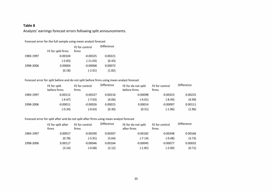
35
Table 8
Analysts’ earnings forecast errors following split announcements.
Forecast error for the full sample using mean analyst forecast
FE for split firms FE for control firms
Difference
1983-1997 -0.00104 -0.00325 0.00221
(-5.83) (-11.03) (6.43)
1998-2006 0.00004 -0.00068 0.00072
(0.18) (-2.01) (1.82)
Forecast error for split before and do not split before firms using mean analyst forecast
FE for split before firms
FE for control firms
Difference FE for do not split before firms
FE for control firms
Difference
1983-1997 -0.00112 -0.00327 0.00216
-0.00098 -0.00323 0.00225
(-4.47) (-7.03) (4.06)
(-4.01) (-8.49) (4.99)
1998-2006 -0.00011 -0.00026 0.00015
0.00014 -0.00097 0.00111
(-0.34) (-0.63) (0.30)
(0.51) (-1.96) (1.96)
Forecast error for split after and do not split after firms using mean analyst forecast
FE for split after firms
FE for control firms
Difference FE for do not split after firms
FE for control firms
Difference
1983-1997 0.00017 -0.00290 0.00307
-0.00182 -0.00348 0.00166
(0.78) (-5.91) (5.64)
(-7.14) (-9.48) (3.73)
1998-2006 0.00117 -0.00046 0.00164
-0.00045 -0.00077 0.00032
(3.14) (-0.68) (2.12)
(-1.85) (-2.00) (0.71)
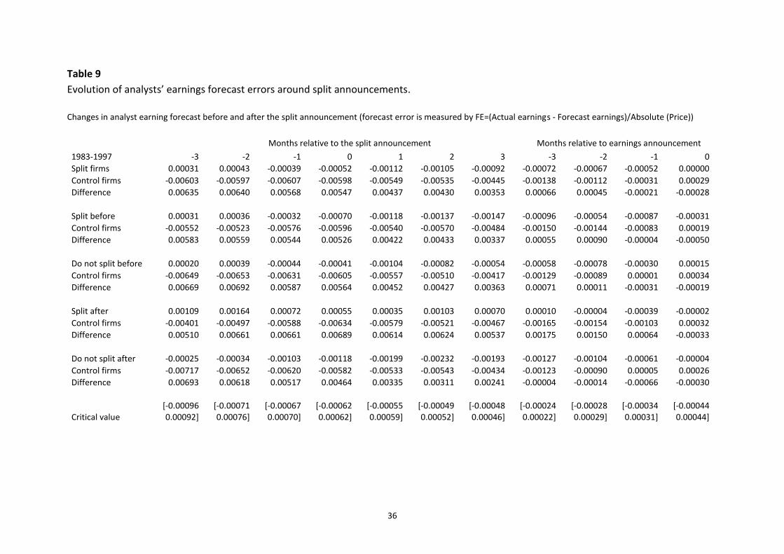
36
Table 9
Evolution of analysts’ earnings forecast errors around split announcements.
Changes in analyst earning forecast before and after the split announcement (forecast error is measured by FE=(Actual earnings - Forecast earnings)/Absolute (Price))
Months relative to the split announcement Months relative to earnings announcement
1983-1997 -3 -2 -1 0 1 2 3 -3 -2 -1 0
Split firms 0.00031 0.00043 -0.00039 -0.00052 -0.00112 -0.00105 -0.00092 -0.00072 -0.00067 -0.00052 0.00000
Control firms -0.00603 -0.00597 -0.00607 -0.00598 -0.00549 -0.00535 -0.00445 -0.00138 -0.00112 -0.00031 0.00029
Difference 0.00635 0.00640 0.00568 0.00547 0.00437 0.00430 0.00353 0.00066 0.00045 -0.00021 -0.00028
Split before 0.00031 0.00036 -0.00032 -0.00070 -0.00118 -0.00137 -0.00147 -0.00096 -0.00054 -0.00087 -0.00031
Control firms -0.00552 -0.00523 -0.00576 -0.00596 -0.00540 -0.00570 -0.00484 -0.00150 -0.00144 -0.00083 0.00019
Difference 0.00583 0.00559 0.00544 0.00526 0.00422 0.00433 0.00337 0.00055 0.00090 -0.00004 -0.00050
Do not split before 0.00020 0.00039 -0.00044 -0.00041 -0.00104 -0.00082 -0.00054 -0.00058 -0.00078 -0.00030 0.00015
Control firms -0.00649 -0.00653 -0.00631 -0.00605 -0.00557 -0.00510 -0.00417 -0.00129 -0.00089 0.00001 0.00034
Difference 0.00669 0.00692 0.00587 0.00564 0.00452 0.00427 0.00363 0.00071 0.00011 -0.00031 -0.00019
Split after 0.00109 0.00164 0.00072 0.00055 0.00035 0.00103 0.00070 0.00010 -0.00004 -0.00039 -0.00002
Control firms -0.00401 -0.00497 -0.00588 -0.00634 -0.00579 -0.00521 -0.00467 -0.00165 -0.00154 -0.00103 0.00032
Difference 0.00510 0.00661 0.00661 0.00689 0.00614 0.00624 0.00537 0.00175 0.00150 0.00064 -0.00033
Do not split after -0.00025 -0.00034 -0.00103 -0.00118 -0.00199 -0.00232 -0.00193 -0.00127 -0.00104 -0.00061 -0.00004
Control firms -0.00717 -0.00652 -0.00620 -0.00582 -0.00533 -0.00543 -0.00434 -0.00123 -0.00090 0.00005 0.00026
Difference 0.00693 0.00618 0.00517 0.00464 0.00335 0.00311 0.00241 -0.00004 -0.00014 -0.00066 -0.00030
Critical value
[-0.00096 0.00092]
[-0.00071 0.00076]
[-0.00067 0.00070]
[-0.00062 0.00062]
[-0.00055 0.00059]
[-0.00049 0.00052]
[-0.00048 0.00046]
[-0.00024 0.00022]
[-0.00028 0.00029]
[-0.00034 0.00031]
[-0.00044 0.00044]

37
1998-2006 Split firms 0.00183 0.00149 0.00227 0.00182 0.00118 0.00130 0.00031 -0.00010 -0.00006 0.00023 0.00023
Control firms -0.00251 -0.00055 -0.00177 -0.00198 -0.00214 -0.00203 -0.00130 0.00044 -0.00032 0.00016 0.00075
Difference 0.00434 0.00205 0.00404 0.00380 0.00333 0.00333 0.00161 -0.00054 0.00026 0.00008 -0.00052
Split before 0.00188 0.00057 0.00237 0.00167 0.00012 0.00139 -0.00005 -0.00016 -0.00006 0.00013 -0.00003
Control firms -0.00266 -0.00058 -0.00306 -0.00313 -0.00279 -0.00272 -0.00248 0.00024 -0.00081 0.00018 0.00023
Difference 0.00454 0.00114 0.00543 0.00480 0.00291 0.00411 0.00243 -0.00040 0.00075 -0.00005 -0.00027
Do not split before 0.00178 0.00238 0.00218 0.00195 0.00200 0.00123 0.00062 -0.00005 -0.00006 0.00034 0.00044
Control firms -0.00236 -0.00054 -0.00068 -0.00113 -0.00162 -0.00143 -0.00035 0.00060 0.00007 0.00014 0.00117
Difference 0.00415 0.00292 0.00287 0.00308 0.00362 0.00266 0.00098 -0.00065 -0.00012 0.00020 -0.00073
Split after 0.00127 0.00186 0.00312 0.00268 0.00320 0.00212 0.00161 0.00031 0.00030 0.00053 -0.00010
Control firms 0.00034 0.00137 0.00054 -0.00228 -0.00081 -0.00015 -0.00112 0.00140 0.00092 0.00092 0.00171
Difference 0.00093 0.00048 0.00258 0.00496 0.00401 0.00227 0.00273 -0.00109 -0.00063 -0.00040 -0.00181
Do not split after 0.00202 0.00135 0.00193 0.00150 0.00031 0.00090 -0.00026 -0.00028 -0.00024 0.00010 0.00038
Control firms -0.00344 -0.00129 -0.00260 -0.00187 -0.00269 -0.00278 -0.00134 0.00007 -0.00082 -0.00010 0.00043
Difference 0.00546 0.00263 0.00453 0.00337 0.00300 0.00368 0.00107 -0.00035 0.00058 0.00020 -0.00005
Critical value
[-0.00115 0.00109]
[-0.00107 0.00109]
[-0.00079 0.00076]
[-0.00073 0.00073]
[-0.00066 0.00074]
[-0.00054 0.00056]
[-0.00051 0.00050]
[-0.00024 0.00022]
[-0.00043 0.00046]
[-0.00032 0.00032]
[-0.00039 0.00044]
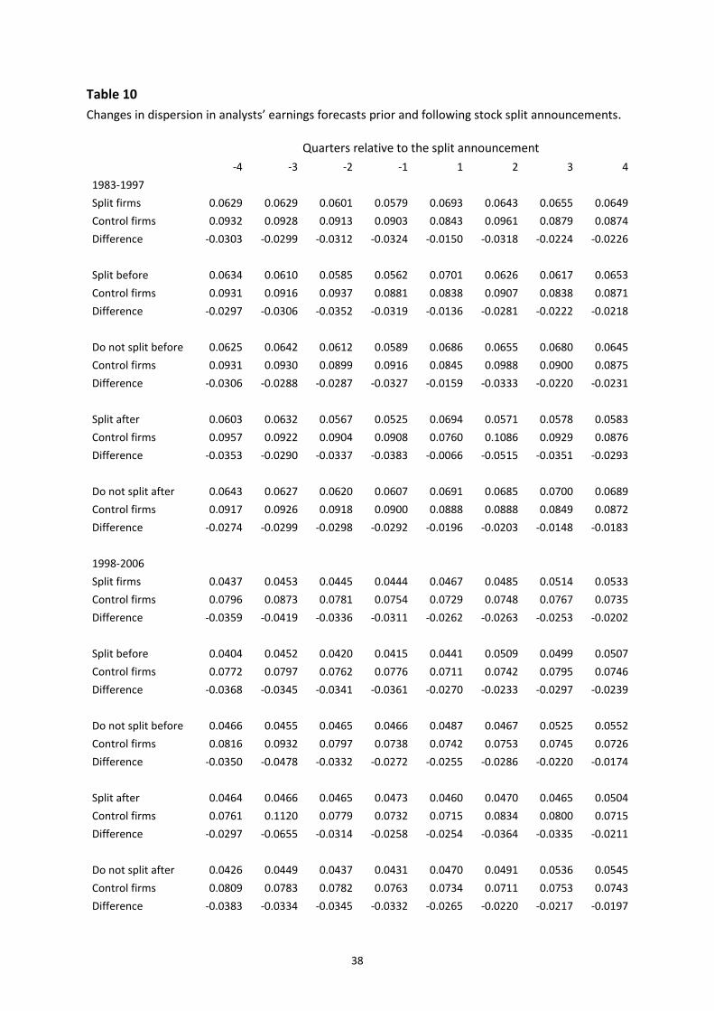
38
Table 10
Changes in dispersion in analysts’ earnings forecasts prior and following stock split announcements.
Quarters relative to the split announcement
-4 -3 -2 -1 1 2 3 4
1983-1997 Split firms 0.0629 0.0629 0.0601 0.0579 0.0693 0.0643 0.0655 0.0649
Control firms 0.0932 0.0928 0.0913 0.0903 0.0843 0.0961 0.0879 0.0874
Difference -0.0303 -0.0299 -0.0312 -0.0324 -0.0150 -0.0318 -0.0224 -0.0226
Split before 0.0634 0.0610 0.0585 0.0562 0.0701 0.0626 0.0617 0.0653
Control firms 0.0931 0.0916 0.0937 0.0881 0.0838 0.0907 0.0838 0.0871
Difference -0.0297 -0.0306 -0.0352 -0.0319 -0.0136 -0.0281 -0.0222 -0.0218
Do not split before 0.0625 0.0642 0.0612 0.0589 0.0686 0.0655 0.0680 0.0645
Control firms 0.0931 0.0930 0.0899 0.0916 0.0845 0.0988 0.0900 0.0875
Difference -0.0306 -0.0288 -0.0287 -0.0327 -0.0159 -0.0333 -0.0220 -0.0231
Split after 0.0603 0.0632 0.0567 0.0525 0.0694 0.0571 0.0578 0.0583
Control firms 0.0957 0.0922 0.0904 0.0908 0.0760 0.1086 0.0929 0.0876
Difference -0.0353 -0.0290 -0.0337 -0.0383 -0.0066 -0.0515 -0.0351 -0.0293
Do not split after 0.0643 0.0627 0.0620 0.0607 0.0691 0.0685 0.0700 0.0689
Control firms 0.0917 0.0926 0.0918 0.0900 0.0888 0.0888 0.0849 0.0872
Difference -0.0274 -0.0299 -0.0298 -0.0292 -0.0196 -0.0203 -0.0148 -0.0183
1998-2006 Split firms 0.0437 0.0453 0.0445 0.0444 0.0467 0.0485 0.0514 0.0533
Control firms 0.0796 0.0873 0.0781 0.0754 0.0729 0.0748 0.0767 0.0735
Difference -0.0359 -0.0419 -0.0336 -0.0311 -0.0262 -0.0263 -0.0253 -0.0202
Split before 0.0404 0.0452 0.0420 0.0415 0.0441 0.0509 0.0499 0.0507
Control firms 0.0772 0.0797 0.0762 0.0776 0.0711 0.0742 0.0795 0.0746
Difference -0.0368 -0.0345 -0.0341 -0.0361 -0.0270 -0.0233 -0.0297 -0.0239
Do not split before 0.0466 0.0455 0.0465 0.0466 0.0487 0.0467 0.0525 0.0552
Control firms 0.0816 0.0932 0.0797 0.0738 0.0742 0.0753 0.0745 0.0726
Difference -0.0350 -0.0478 -0.0332 -0.0272 -0.0255 -0.0286 -0.0220 -0.0174
Split after 0.0464 0.0466 0.0465 0.0473 0.0460 0.0470 0.0465 0.0504
Control firms 0.0761 0.1120 0.0779 0.0732 0.0715 0.0834 0.0800 0.0715
Difference -0.0297 -0.0655 -0.0314 -0.0258 -0.0254 -0.0364 -0.0335 -0.0211
Do not split after 0.0426 0.0449 0.0437 0.0431 0.0470 0.0491 0.0536 0.0545
Control firms 0.0809 0.0783 0.0782 0.0763 0.0734 0.0711 0.0753 0.0743
Difference -0.0383 -0.0334 -0.0345 -0.0332 -0.0265 -0.0220 -0.0217 -0.0197
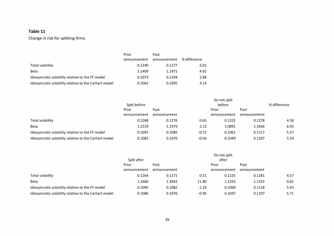
39
Table 11
Change in risk for splitting firms.
Prior announcement
Post announcement % difference
Total volatility 0.1240 0.1277 3.01 Beta 1.1409 1.1971 4.92 Idiosyncratic volatility relative to the FF model 0.1073 0.1104 2.88 Idiosyncratic volatility relative to the Carhart model 0.1062 0.1095 3.14
Split before
Do not split before
% difference
Prior announcement
Post announcement
Prior announcement
Post announcement
Total volatility 0.1268 0.1276 0.65 0.1222 0.1278 4.58
Beta 1.2219 1.2479 2.13 1.0891 1.1646 6.93
Idiosyncratic volatility relative to the FF model 0.1092 0.1085 -0.72 0.1061 0.1117 5.27
Idiosyncratic volatility relative to the Carhart model 0.1082 0.1076 -0.56 0.1049 0.1107 5.59
Split after
Do not split after
Prior announcement
Post announcement
Prior announcement
Post announcement
Total volatility 0.1264 0.1271 0.51 0.1225 0.1281 4.57
Beta 1.1666 1.3042 11.80 1.1255 1.1325 0.62
Idiosyncratic volatility relative to the FF model 0.1095 0.1082 -1.19 0.1060 0.1118 5.43
Idiosyncratic volatility relative to the Carhart model 0.1086 0.1076 -0.95 0.1047 0.1107 5.71
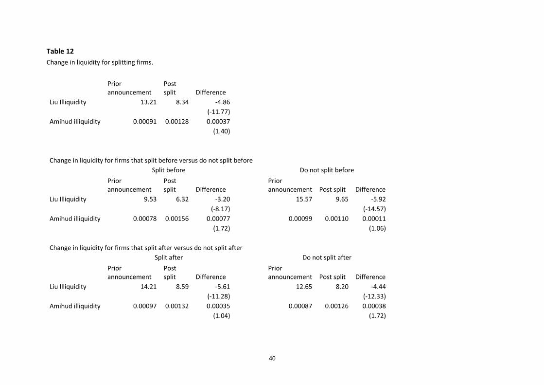
40
Table 12
Change in liquidity for splitting firms.
Prior announcement
Post split Difference
Liu Illiquidity 13.21 8.34 -4.86
(-11.77)
Amihud illiquidity 0.00091 0.00128 0.00037
(1.40)
Change in liquidity for firms that split before versus do not split before
Split before
Do not split before
Prior announcement
Post split Difference
Prior announcement Post split Difference
Liu Illiquidity 9.53 6.32 -3.20
15.57 9.65 -5.92
(-8.17)
(-14.57)
Amihud illiquidity 0.00078 0.00156 0.00077
0.00099 0.00110 0.00011
(1.72)
(1.06)
Change in liquidity for firms that split after versus do not split after
Split after
Do not split after
Prior announcement
Post split Difference
Prior announcement Post split Difference
Liu Illiquidity 14.21 8.59 -5.61
12.65 8.20 -4.44
(-11.28)
(-12.33)
Amihud illiquidity 0.00097 0.00132 0.00035
0.00087 0.00126 0.00038
(1.04)
(1.72)
Recommended