T.Y.B.Com Sem-VI : 2020-21
Prof. Anil KhadseSheth N.K.T.T College,Thane
Anil Khadse NKTT College,Thane
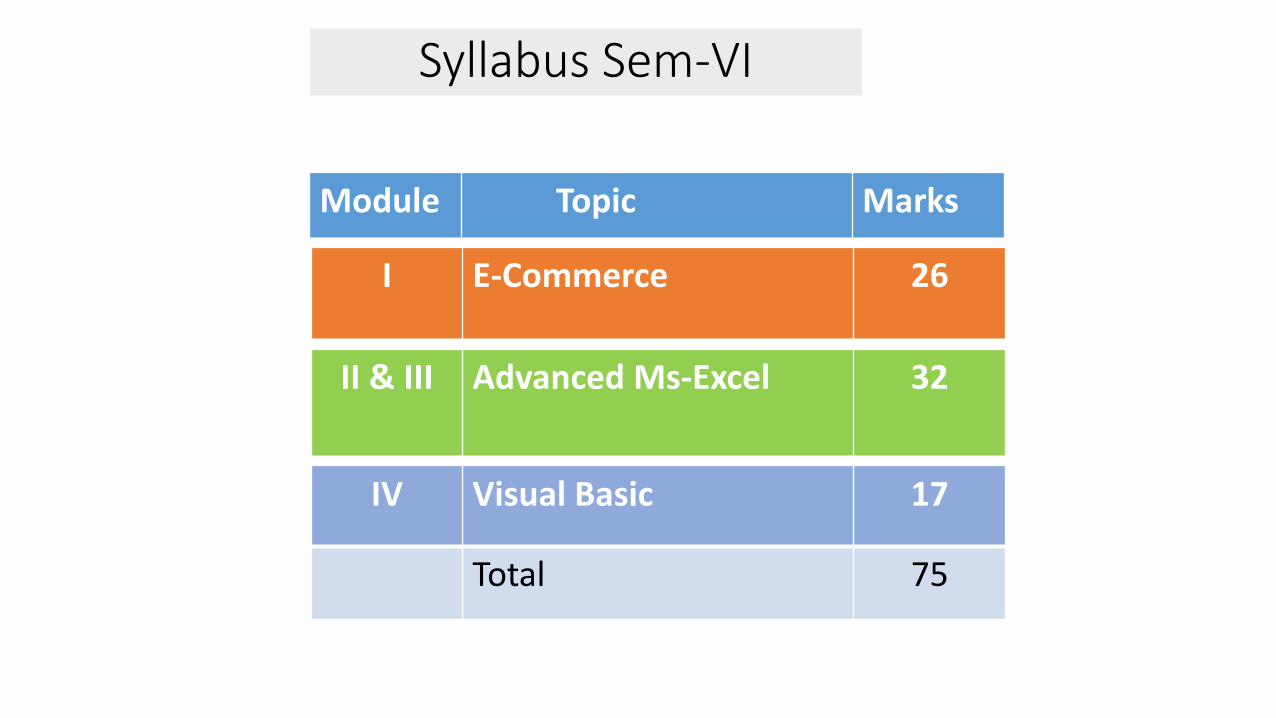
Syllabus Sem-VI
IV Visual Basic 17
Total 75
Module Topic Marks
I E-Commerce 26
II & III Advanced Ms-Excel 32
Anil Khadse NKTT College,Thane
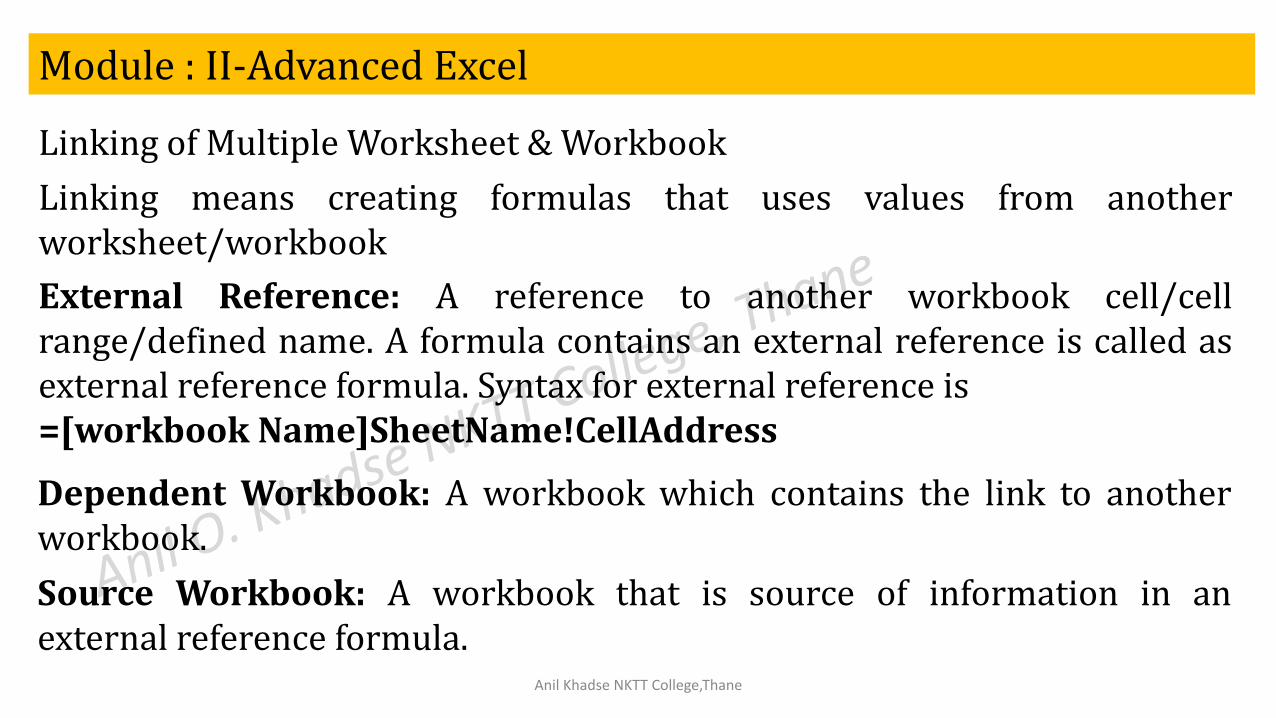
Module : II-Advanced Excel
Linking of Multiple Worksheet & Workbook
Linking means creating formulas that uses values from anotherworksheet/workbook
External Reference: A reference to another workbook cell/cellrange/defined name. A formula contains an external reference is called asexternal reference formula. Syntax for external reference is=[workbook Name]SheetName!CellAddress
Dependent Workbook: A workbook which contains the link to anotherworkbook.
Source Workbook: A workbook that is source of information in anexternal reference formula.
Anil Khadse NKTT College,Thane
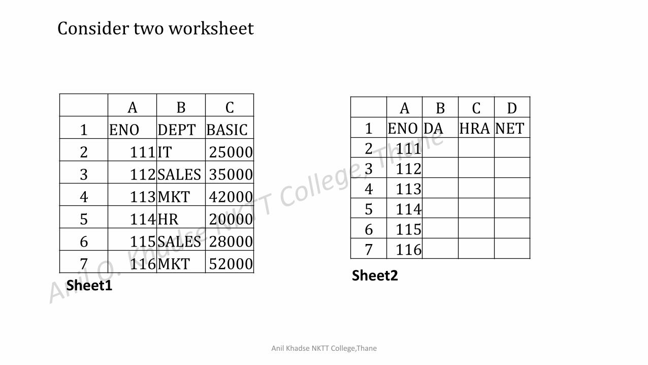
A B C
1 ENO DEPT BASIC
2 111IT 25000
3 112SALES 35000
4 113MKT 42000
5 114HR 20000
6 115SALES 28000
7 116MKT 52000
A B C D1 ENO DA HRA NET2 1113 1124 1135 1146 1157 116
Consider two worksheet
Sheet1Sheet2
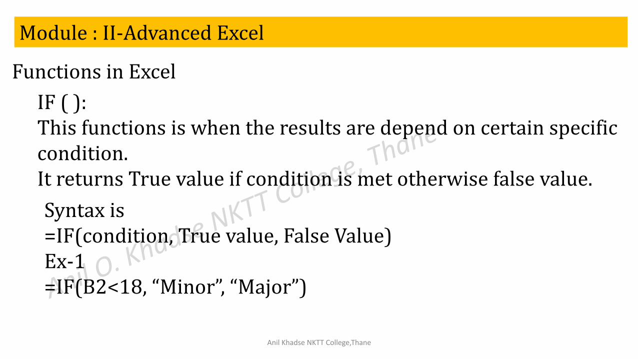
Functions in Excel
IF ( ):This functions is when the results are depend on certain specific condition.It returns True value if condition is met otherwise false value.
Syntax is=IF(condition, True value, False Value)Ex-1=IF(B2<18, “Minor”, “Major”)
Module : II-Advanced Excel
Anil Khadse NKTT College,Thane
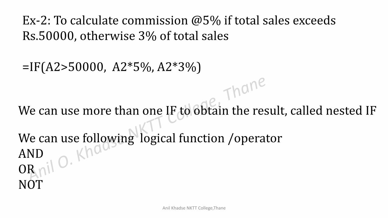
Ex-2: To calculate commission @5% if total sales exceeds Rs.50000, otherwise 3% of total sales
=IF(A2>50000, A2*5%, A2*3%)
We can use more than one IF to obtain the result, called nested IF
Anil Khadse NKTT College,Thane
We can use following logical function /operatorANDORNOT
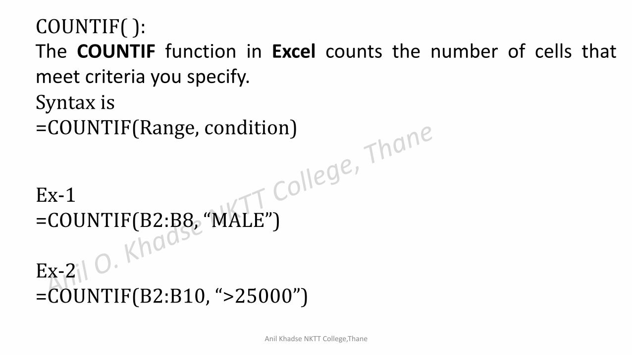
Ex-1=COUNTIF(B2:B8, “MALE”)
Ex-2=COUNTIF(B2:B10, “>25000”)
COUNTIF( ):The COUNTIF function in Excel counts the number of cells thatmeet criteria you specify.Syntax is=COUNTIF(Range, condition)
Anil Khadse NKTT College,Thane
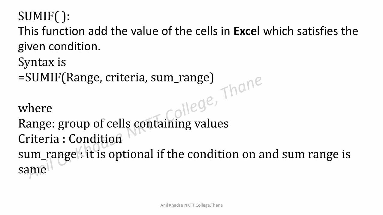
SUMIF( ):This function add the value of the cells in Excel which satisfies the given condition.Syntax is=SUMIF(Range, criteria, sum_range)
whereRange: group of cells containing values Criteria : Condition sum_range : it is optional if the condition on and sum range is same
Anil Khadse NKTT College,Thane
AVERAGEIF( ):This function used to find the average/ Arithmetic Mean of the numbers entered in the cells which satisfies the given condition.Syntax is=AVERAGEIF(Range, criteria, average_range)
Anil Khadse NKTT College,Thane
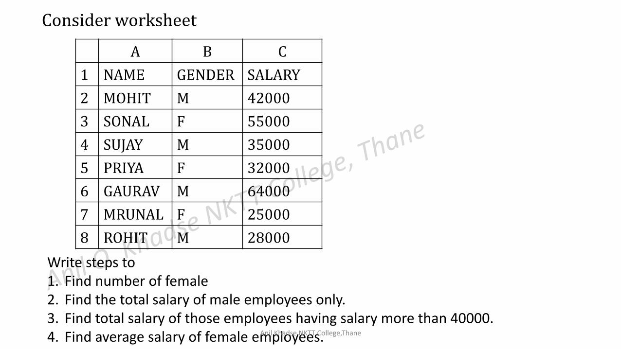
A B C
1 NAME GENDER SALARY
2 MOHIT M 42000
3 SONAL F 55000
4 SUJAY M 35000
5 PRIYA F 32000
6 GAURAV M 64000
7 MRUNAL F 25000
8 ROHIT M 28000
Consider worksheet
Write steps to1. Find number of female 2. Find the total salary of male employees only.3. Find total salary of those employees having salary more than 40000.4. Find average salary of female employees.Anil Khadse NKTT College,Thane
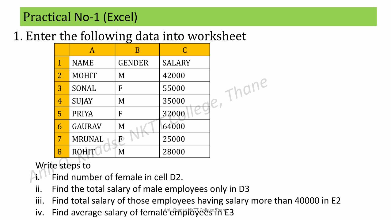
Practical No-1 (Excel)
1. Enter the following data into worksheetA B C
1 NAME GENDER SALARY
2 MOHIT M 42000
3 SONAL F 55000
4 SUJAY M 35000
5 PRIYA F 32000
6 GAURAV M 64000
7 MRUNAL F 25000
8 ROHIT M 28000
Write steps toi. Find number of female in cell D2.ii. Find the total salary of male employees only in D3iii. Find total salary of those employees having salary more than 40000 in E2 iv. Find average salary of female employees in E3Anil Khadse NKTT College,Thane
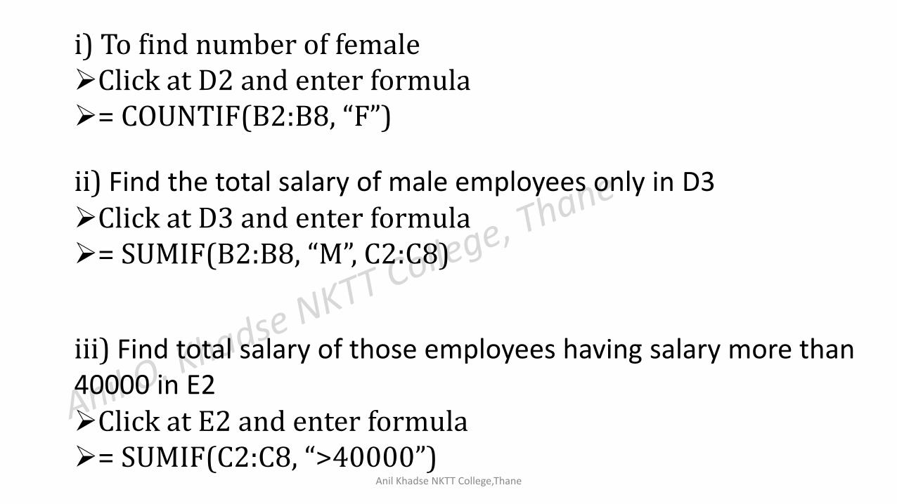
i) To find number of femaleClick at D2 and enter formula= COUNTIF(B2:B8, “F”)
ii) Find the total salary of male employees only in D3Click at D3 and enter formula= SUMIF(B2:B8, “M”, C2:C8)
iii) Find total salary of those employees having salary more than 40000 in E2Click at E2 and enter formula= SUMIF(C2:C8, “>40000”)
Anil Khadse NKTT College,Thane
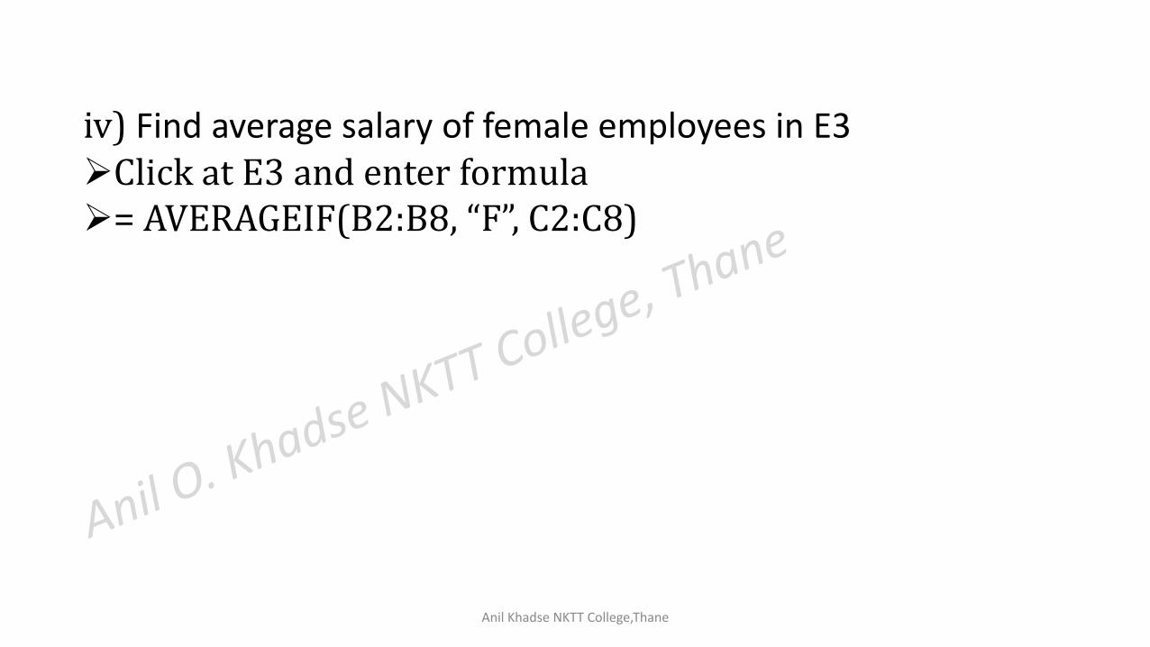
iv) Find average salary of female employees in E3Click at E3 and enter formula= AVERAGEIF(B2:B8, “F”, C2:C8)
Anil Khadse NKTT College,Thane
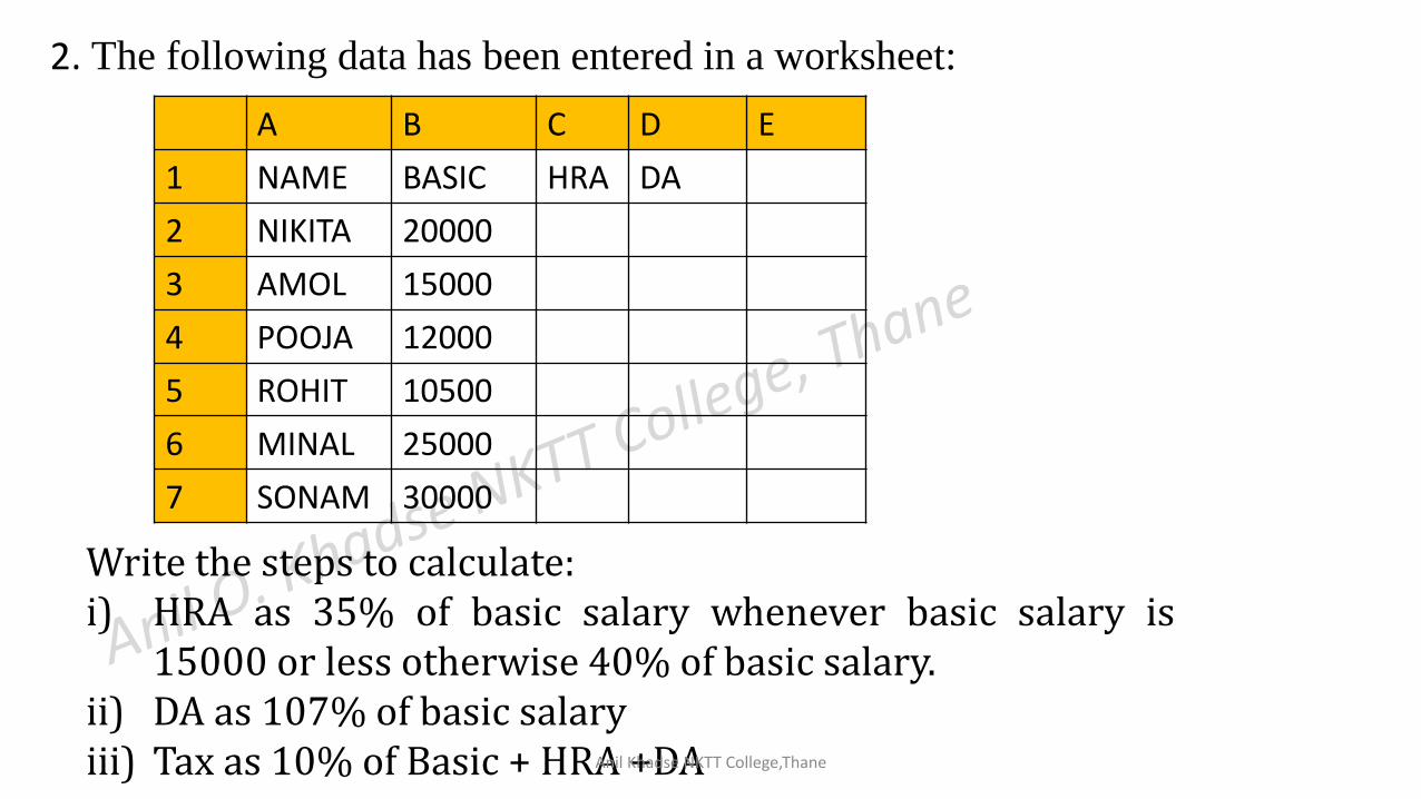
2. The following data has been entered in a worksheet:
A B C D E
1 NAME BASIC HRA DA
2 NIKITA 20000
3 AMOL 15000
4 POOJA 12000
5 ROHIT 10500
6 MINAL 25000
7 SONAM 30000
Write the steps to calculate:i) HRA as 35% of basic salary whenever basic salary is
15000 or less otherwise 40% of basic salary.ii) DA as 107% of basic salaryiii) Tax as 10% of Basic + HRA +DAAnil Khadse NKTT College,Thane
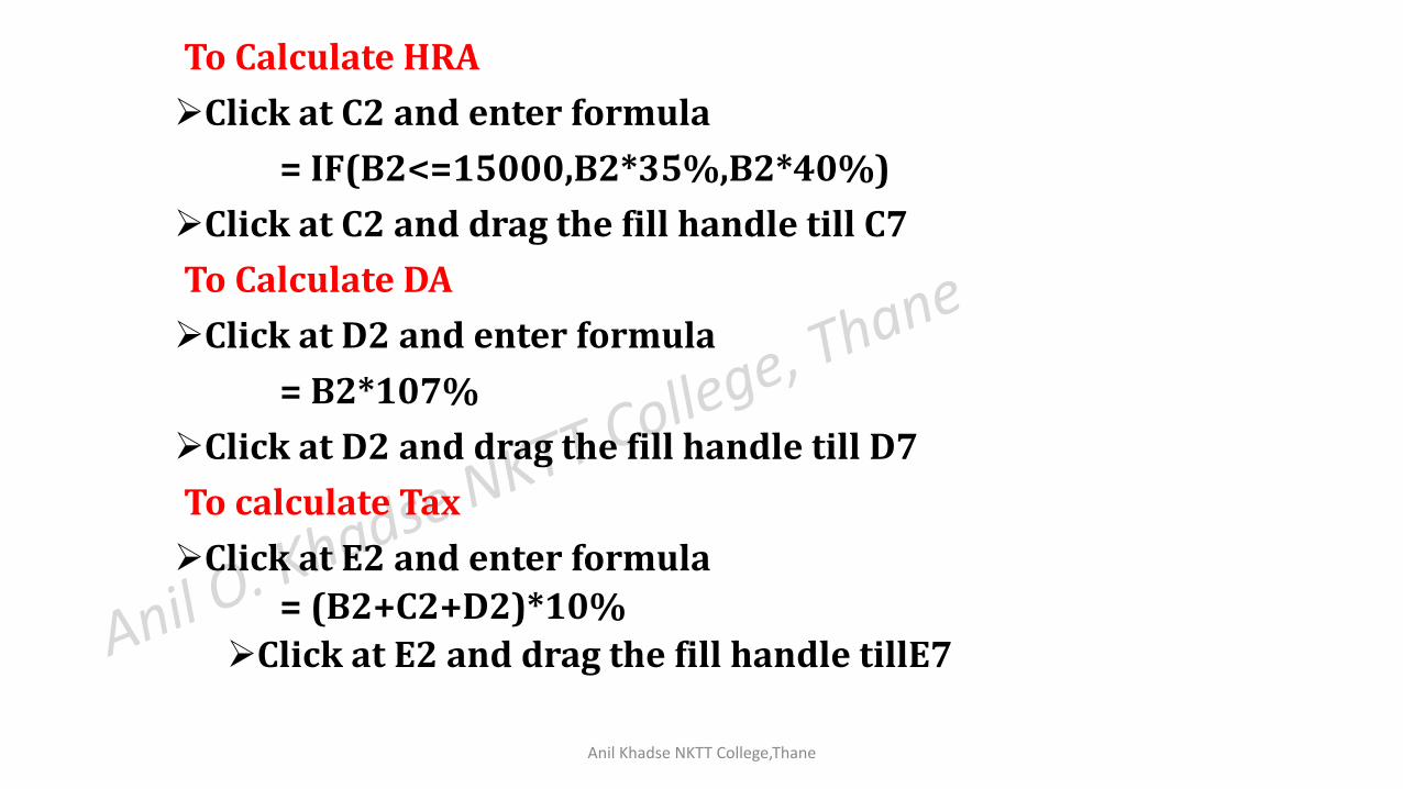
To Calculate HRA
Click at C2 and enter formula
= IF(B2<=15000,B2*35%,B2*40%)
Click at C2 and drag the fill handle till C7
To Calculate DA
Click at D2 and enter formula
= B2*107%
Click at D2 and drag the fill handle till D7
To calculate Tax
Click at E2 and enter formula
= (B2+C2+D2)*10%
Click at E2 and drag the fill handle tillE7
Anil Khadse NKTT College,Thane
Anil Khadse NKTT College,Thane
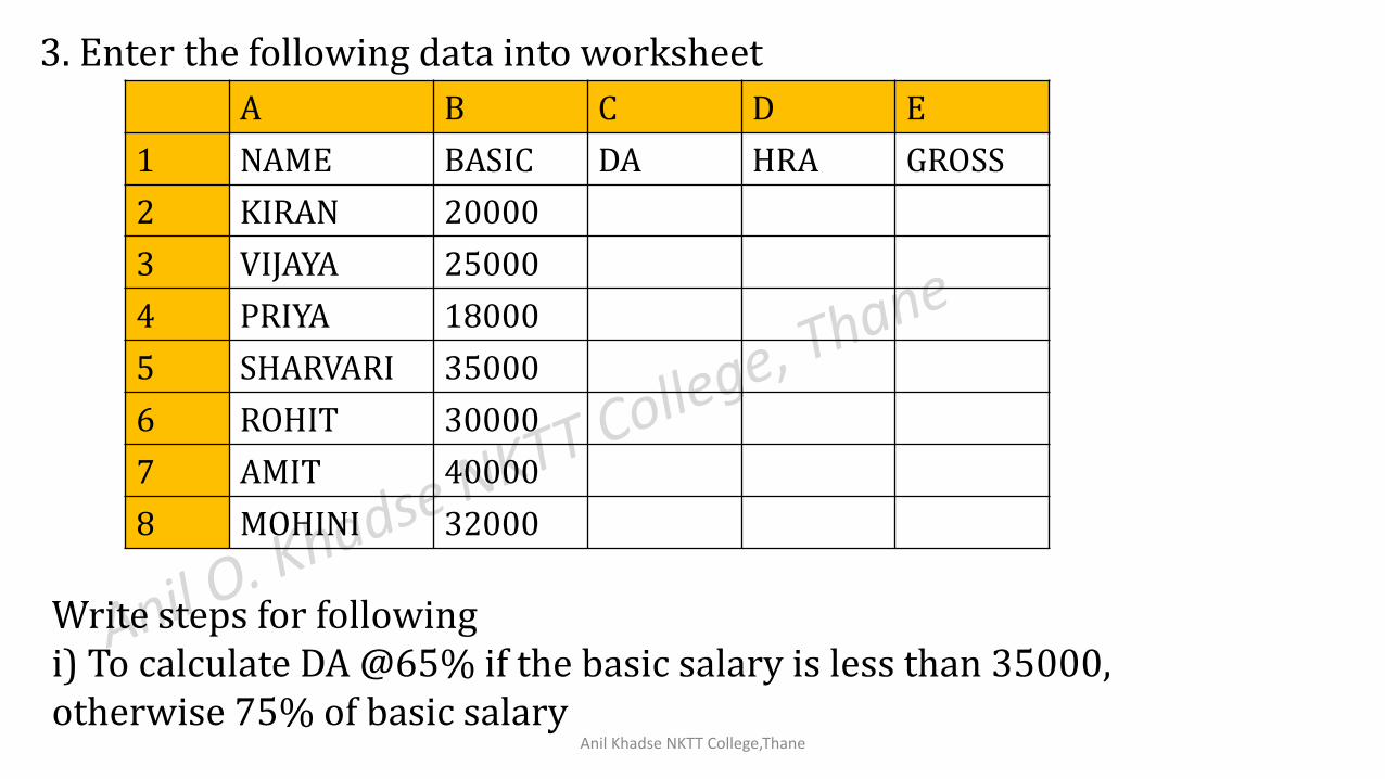
3. Enter the following data into worksheet
A B C D E
1 NAME BASIC DA HRA GROSS
2 KIRAN 20000
3 VIJAYA 25000
4 PRIYA 18000
5 SHARVARI 35000
6 ROHIT 30000
7 AMIT 40000
8 MOHINI 32000
Write steps for followingi) To calculate DA @65% if the basic salary is less than 35000, otherwise 75% of basic salary
Anil Khadse NKTT College,Thane
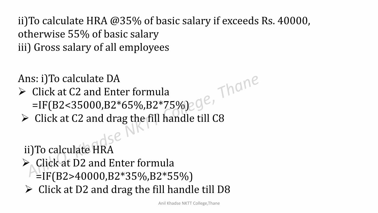
ii)To calculate HRA @35% of basic salary if exceeds Rs. 40000, otherwise 55% of basic salaryiii) Gross salary of all employees
Ans: i)To calculate DA Click at C2 and Enter formula
=IF(B2<35000,B2*65%,B2*75%) Click at C2 and drag the fill handle till C8
ii)To calculate HRA Click at D2 and Enter formula
=IF(B2>40000,B2*35%,B2*55%) Click at D2 and drag the fill handle till D8
Anil Khadse NKTT College,Thane
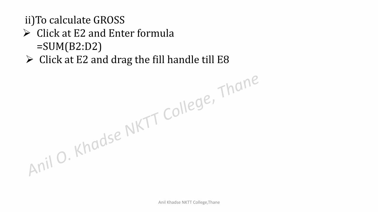
ii)To calculate GROSS Click at E2 and Enter formula
=SUM(B2:D2) Click at E2 and drag the fill handle till E8
Anil Khadse NKTT College,Thane
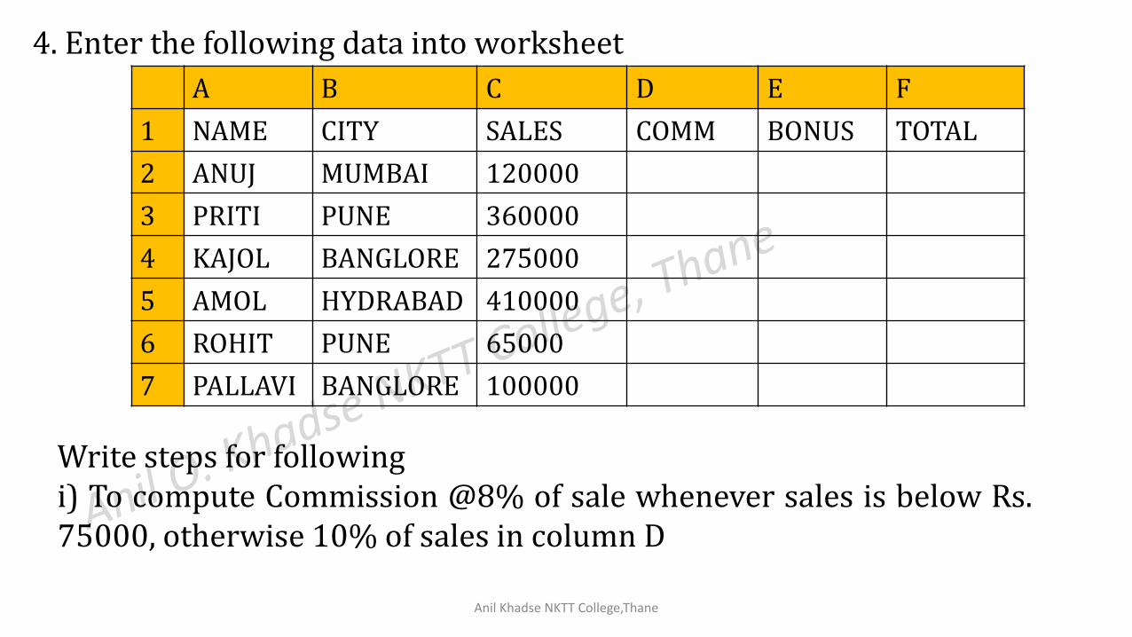
4. Enter the following data into worksheet
A B C D E F
1 NAME CITY SALES COMM BONUS TOTAL
2 ANUJ MUMBAI 120000
3 PRITI PUNE 360000
4 KAJOL BANGLORE 275000
5 AMOL HYDRABAD 410000
6 ROHIT PUNE 65000
7 PALLAVI BANGLORE 100000
Write steps for followingi) To compute Commission @8% of sale whenever sales is below Rs.75000, otherwise 10% of sales in column D
Anil Khadse NKTT College,Thane
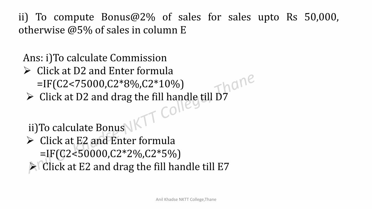
ii) To compute Bonus@2% of sales for sales upto Rs 50,000,otherwise @5% of sales in column E
Ans: i)To calculate Commission Click at D2 and Enter formula
=IF(C2<75000,C2*8%,C2*10%) Click at D2 and drag the fill handle till D7
ii)To calculate Bonus Click at E2 and Enter formula
=IF(C2<50000,C2*2%,C2*5%) Click at E2 and drag the fill handle till E7

Anil Khadse NKTT College,Thane
ii)To calculate Total earning Click at F2 and Enter formula
=D2+E2 Click at F2 and drag the fill handle till F7
End of Practical 1
Anil Khadse NKTT College,Thane
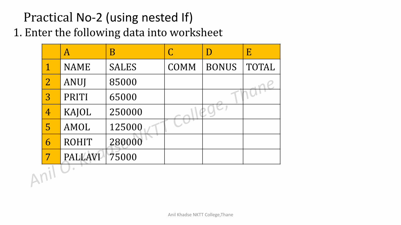
Practical No-2 (using nested If)1. Enter the following data into worksheet
A B C D E
1 NAME SALES COMM BONUS TOTAL
2 ANUJ 85000
3 PRITI 65000
4 KAJOL 250000
5 AMOL 125000
6 ROHIT 280000
7 PALLAVI 75000
Anil Khadse NKTT College,Thane
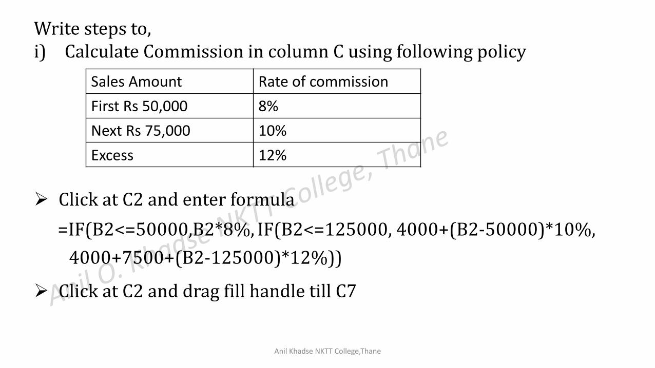
Write steps to,i) Calculate Commission in column C using following policy
Sales Amount Rate of commission
First Rs 50,000 8%
Next Rs 75,000 10%
Excess 12%
Click at C2 and enter formula
Click at C2 and drag fill handle till C7
=IF(B2<=50000,B2*8%, IF(B2<=125000, 4000+(B2-50000)*10%,
4000+7500+(B2-125000)*12%))
Anil Khadse NKTT College,Thane
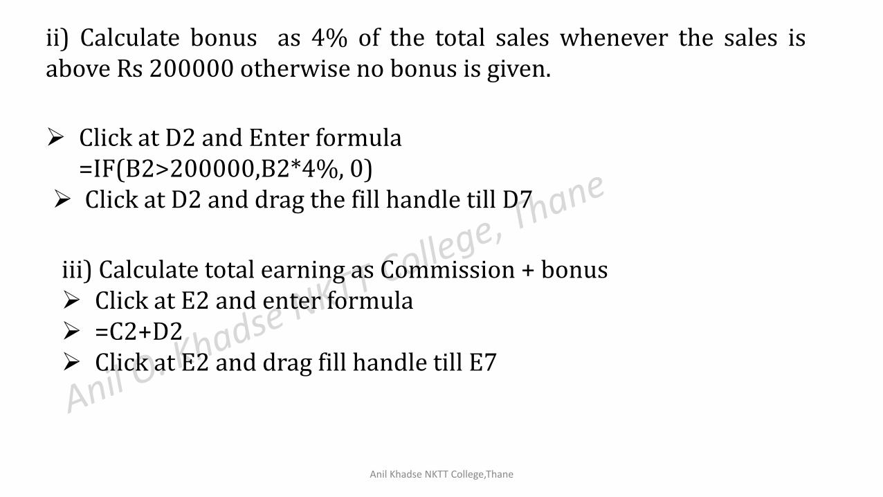
ii) Calculate bonus as 4% of the total sales whenever the sales isabove Rs 200000 otherwise no bonus is given.
Click at D2 and Enter formula=IF(B2>200000,B2*4%, 0)
Click at D2 and drag the fill handle till D7
iii) Calculate total earning as Commission + bonus Click at E2 and enter formula =C2+D2 Click at E2 and drag fill handle till E7
Anil Khadse NKTT College,Thane
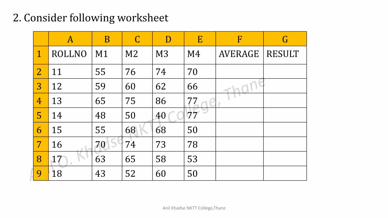
2. Consider following worksheet
A B C D E F G
1 ROLLNO M1 M2 M3 M4 AVERAGE RESULT
2 11 55 76 74 70
3 12 59 60 62 66
4 13 65 75 86 77
5 14 48 50 40 77
6 15 55 68 68 50
7 16 70 74 73 78
8 17 63 65 58 53
9 18 43 52 60 50
Anil Khadse NKTT College,Thane
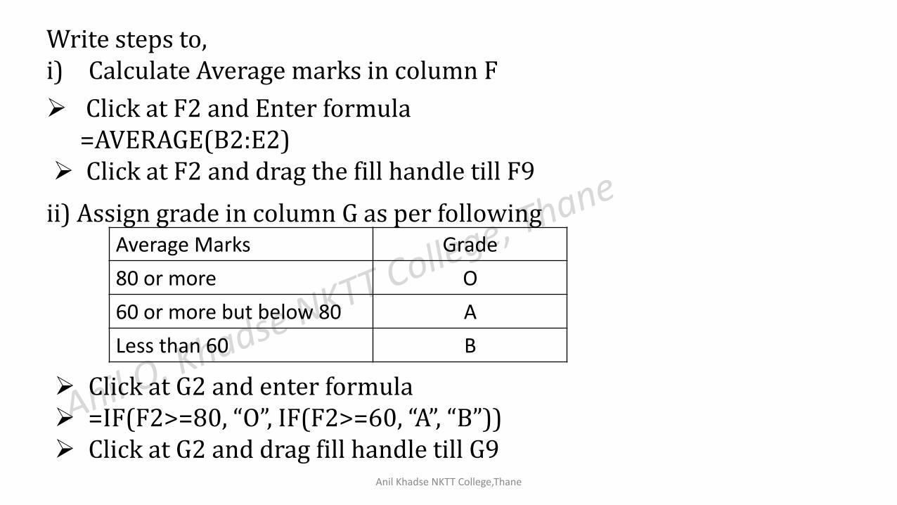
Write steps to,i) Calculate Average marks in column F
Click at F2 and Enter formula=AVERAGE(B2:E2)
Click at F2 and drag the fill handle till F9
ii) Assign grade in column G as per followingAverage Marks Grade
80 or more O
60 or more but below 80 A
Less than 60 B
Click at G2 and enter formula =IF(F2>=80, “O”, IF(F2>=60, “A”, “B”)) Click at G2 and drag fill handle till G9
Anil Khadse NKTT College,Thane
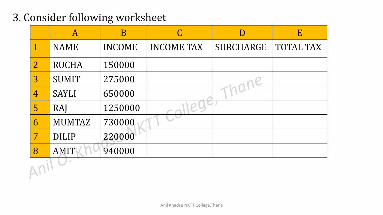
3. Consider following worksheet
A B C D E
1 NAME INCOME INCOME TAX SURCHARGE TOTAL TAX
2 RUCHA 150000
3 SUMIT 275000
4 SAYLI 650000
5 RAJ 1250000
6 MUMTAZ 730000
7 DILIP 220000
8 AMIT 940000
Anil Khadse NKTT College,Thane
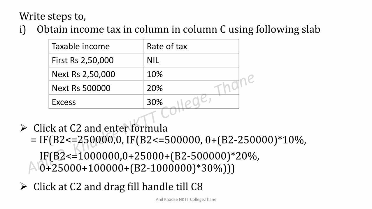
Write steps to,i) Obtain income tax in column in column C using following slab
Taxable income Rate of tax
First Rs 2,50,000 NIL
Next Rs 2,50,000 10%
Next Rs 500000 20%
Excess 30%
Click at C2 and enter formula
Click at C2 and drag fill handle till C8
= IF(B2<=250000,0, IF(B2<=500000, 0+(B2-250000)*10%,
IF(B2<=1000000,0+25000+(B2-500000)*20%,0+25000+100000+(B2-1000000)*30%)))
Anil Khadse NKTT College,Thane
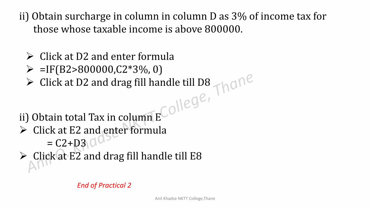
ii) Obtain surcharge in column in column D as 3% of income tax forthose whose taxable income is above 800000.
Click at D2 and enter formula =IF(B2>800000,C2*3%, 0) Click at D2 and drag fill handle till D8
ii) Obtain total Tax in column E Click at E2 and enter formula
= C2+D3 Click at E2 and drag fill handle till E8
End of Practical 2
Anil Khadse NKTT College,Thane
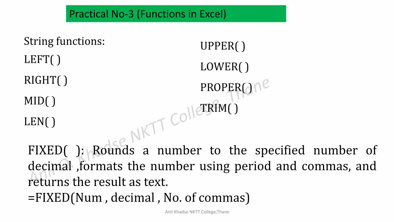
String functions:
LEFT( )
RIGHT( )
MID( )
LEN( )
Practical No-3 (Functions in Excel)
UPPER( )
LOWER( )
PROPER( )
TRIM( )
FIXED( ): Rounds a number to the specified number ofdecimal ,formats the number using period and commas, andreturns the result as text.=FIXED(Num , decimal , No. of commas)
Anil Khadse NKTT College,Thane
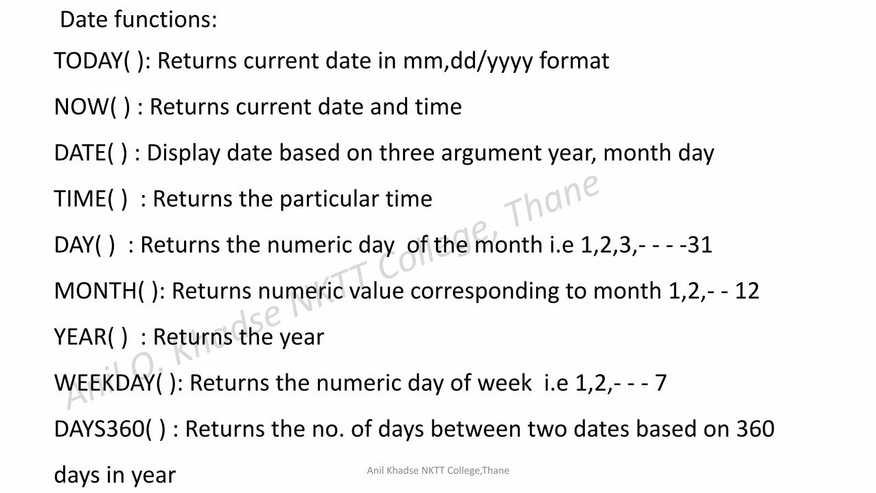
Date functions:
TODAY( ): Returns current date in mm,dd/yyyy format
NOW( ) : Returns current date and time
DATE( ) : Display date based on three argument year, month day
TIME( ) : Returns the particular time
DAY( ) : Returns the numeric day of the month i.e 1,2,3,- - - -31
MONTH( ): Returns numeric value corresponding to month 1,2,- - 12
YEAR( ) : Returns the year
WEEKDAY( ): Returns the numeric day of week i.e 1,2,- - - 7
DAYS360( ) : Returns the no. of days between two dates based on 360
days in year
Anil Khadse NKTT College,Thane
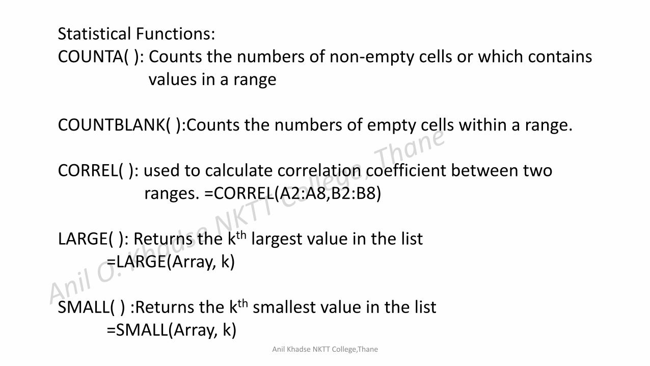
Statistical Functions:COUNTA( ): Counts the numbers of non-empty cells or which contains
values in a range
COUNTBLANK( ):Counts the numbers of empty cells within a range.
CORREL( ): used to calculate correlation coefficient between tworanges. =CORREL(A2:A8,B2:B8)
LARGE( ): Returns the kth largest value in the list=LARGE(Array, k)
SMALL( ) :Returns the kth smallest value in the list=SMALL(Array, k)
Anil Khadse NKTT College,Thane
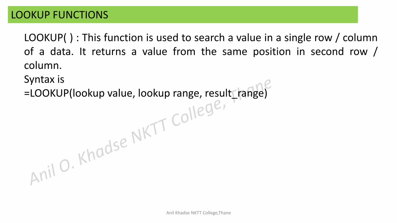
LOOKUP FUNCTIONS
LOOKUP( ) : This function is used to search a value in a single row / columnof a data. It returns a value from the same position in second row /column.Syntax is=LOOKUP(lookup value, lookup range, result_range)
Anil Khadse NKTT College,Thane
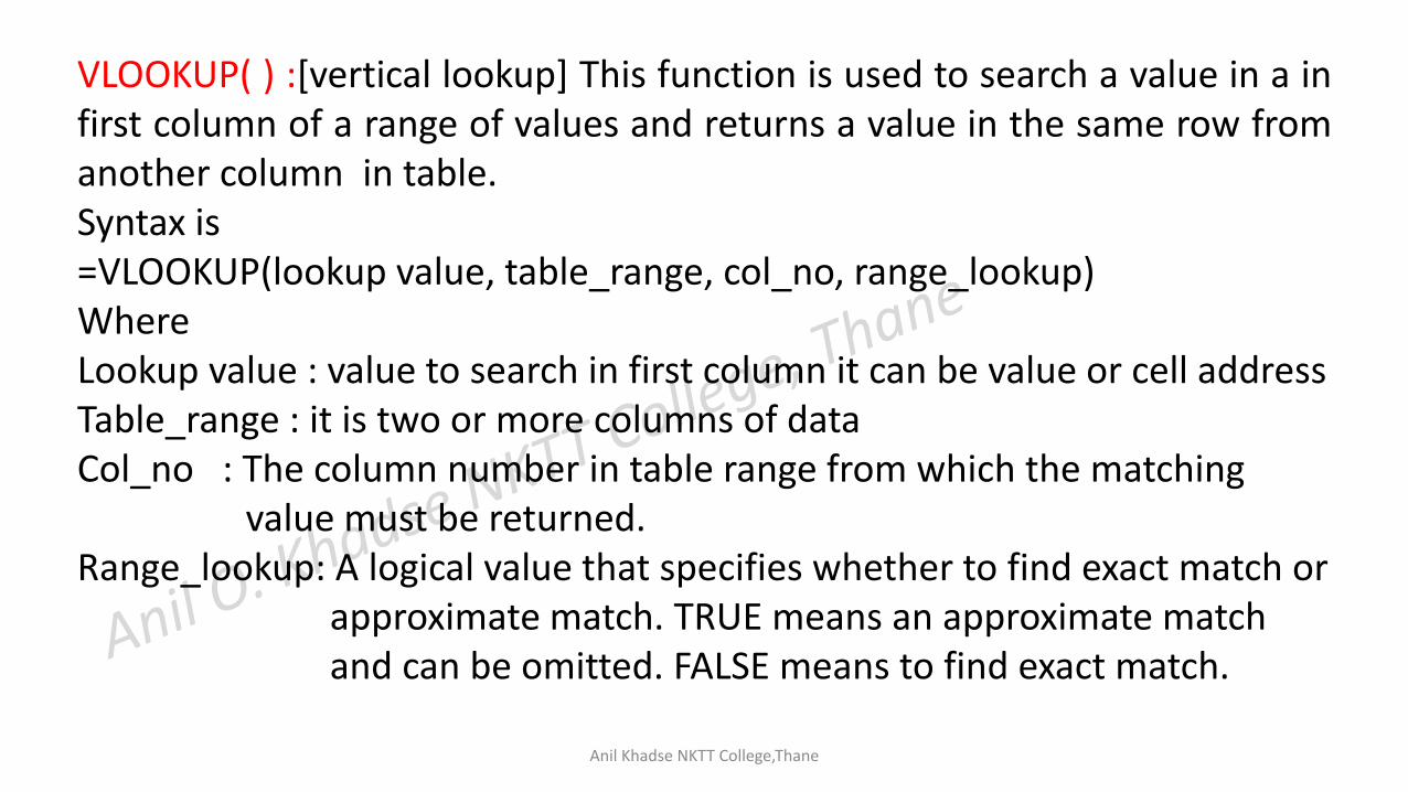
VLOOKUP( ) :[vertical lookup] This function is used to search a value in a infirst column of a range of values and returns a value in the same row fromanother column in table.Syntax is=VLOOKUP(lookup value, table_range, col_no, range_lookup)WhereLookup value : value to search in first column it can be value or cell addressTable_range : it is two or more columns of dataCol_no : The column number in table range from which the matching
value must be returned.Range_lookup: A logical value that specifies whether to find exact match or
approximate match. TRUE means an approximate matchand can be omitted. FALSE means to find exact match.
Anil Khadse NKTT College,Thane
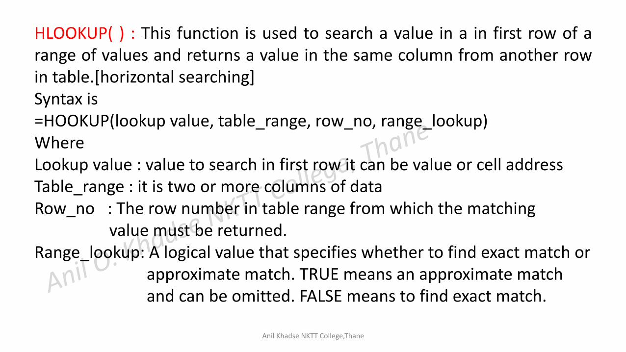
HLOOKUP( ) : This function is used to search a value in a in first row of arange of values and returns a value in the same column from another rowin table.[horizontal searching]Syntax is=HOOKUP(lookup value, table_range, row_no, range_lookup)WhereLookup value : value to search in first row it can be value or cell addressTable_range : it is two or more columns of dataRow_no : The row number in table range from which the matching
value must be returned.Range_lookup: A logical value that specifies whether to find exact match or
approximate match. TRUE means an approximate matchand can be omitted. FALSE means to find exact match.
Anil Khadse NKTT College,Thane
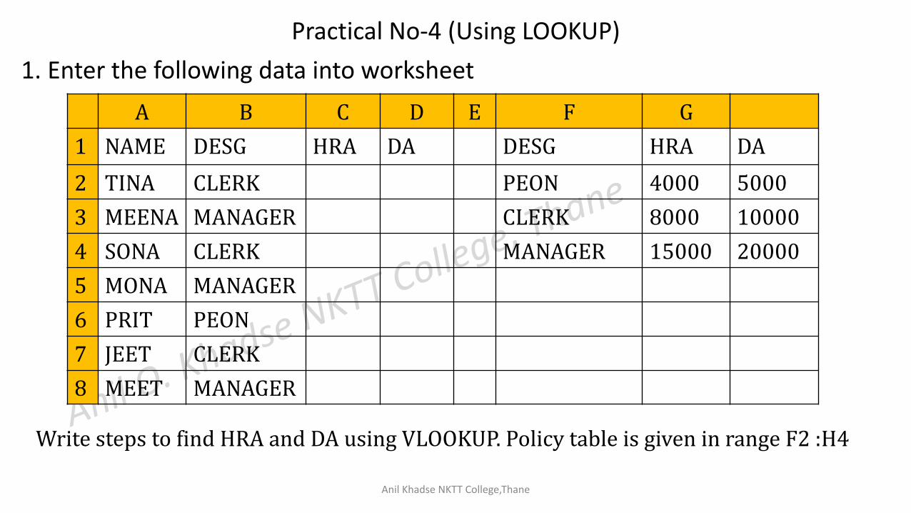
Practical No-4 (Using LOOKUP)
1. Enter the following data into worksheet
A B C D E F G
1 NAME DESG HRA DA DESG HRA DA
2 TINA CLERK PEON 4000 5000
3 MEENA MANAGER CLERK 8000 10000
4 SONA CLERK MANAGER 15000 20000
5 MONA MANAGER
6 PRIT PEON
7 JEET CLERK
8 MEET MANAGER
Write steps to find HRA and DA using VLOOKUP. Policy table is given in range F2 :H4

Anil Khadse NKTT College,Thane
To find HRA
Click at C2 and entered formula
=VLOOKUP(B2,$F$2:$H$4,2)
Click at C2 and drag the fill handle till C8
To find DA
Click at D2 and entered formula
=VLOOKUP(B2,$F$2:$H$4,3)
Click at D2 and drag the fill handle till D8
Anil Khadse NKTT College,Thane
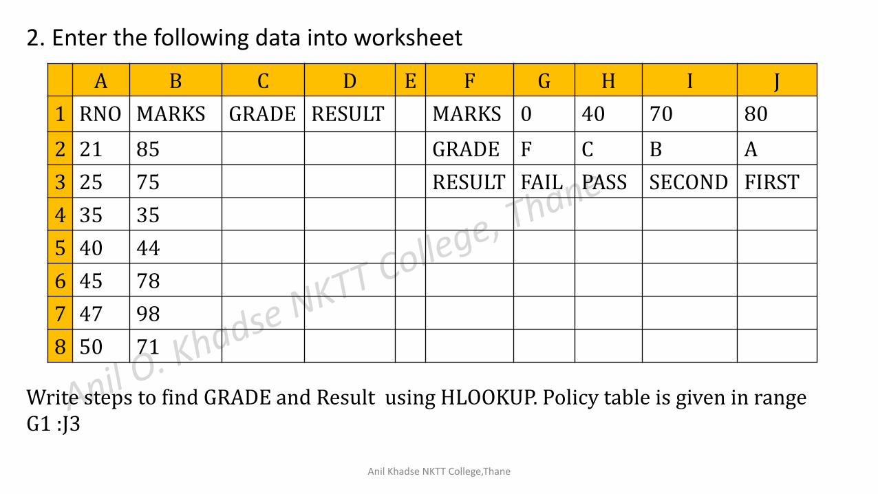
2. Enter the following data into worksheet
A B C D E F G H I J
1 RNO MARKS GRADE RESULT MARKS 0 40 70 80
2 21 85 GRADE F C B A
3 25 75 RESULT FAIL PASS SECOND FIRST
4 35 35
5 40 44
6 45 78
7 47 98
8 50 71
Write steps to find GRADE and Result using HLOOKUP. Policy table is given in range G1 :J3
Anil Khadse NKTT College,Thane
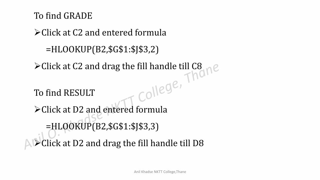
To find GRADE
Click at C2 and entered formula
=HLOOKUP(B2,$G$1:$J$3,2)
Click at C2 and drag the fill handle till C8
To find RESULT
Click at D2 and entered formula
=HLOOKUP(B2,$G$1:$J$3,3)
Click at D2 and drag the fill handle till D8
Anil Khadse NKTT College,Thane
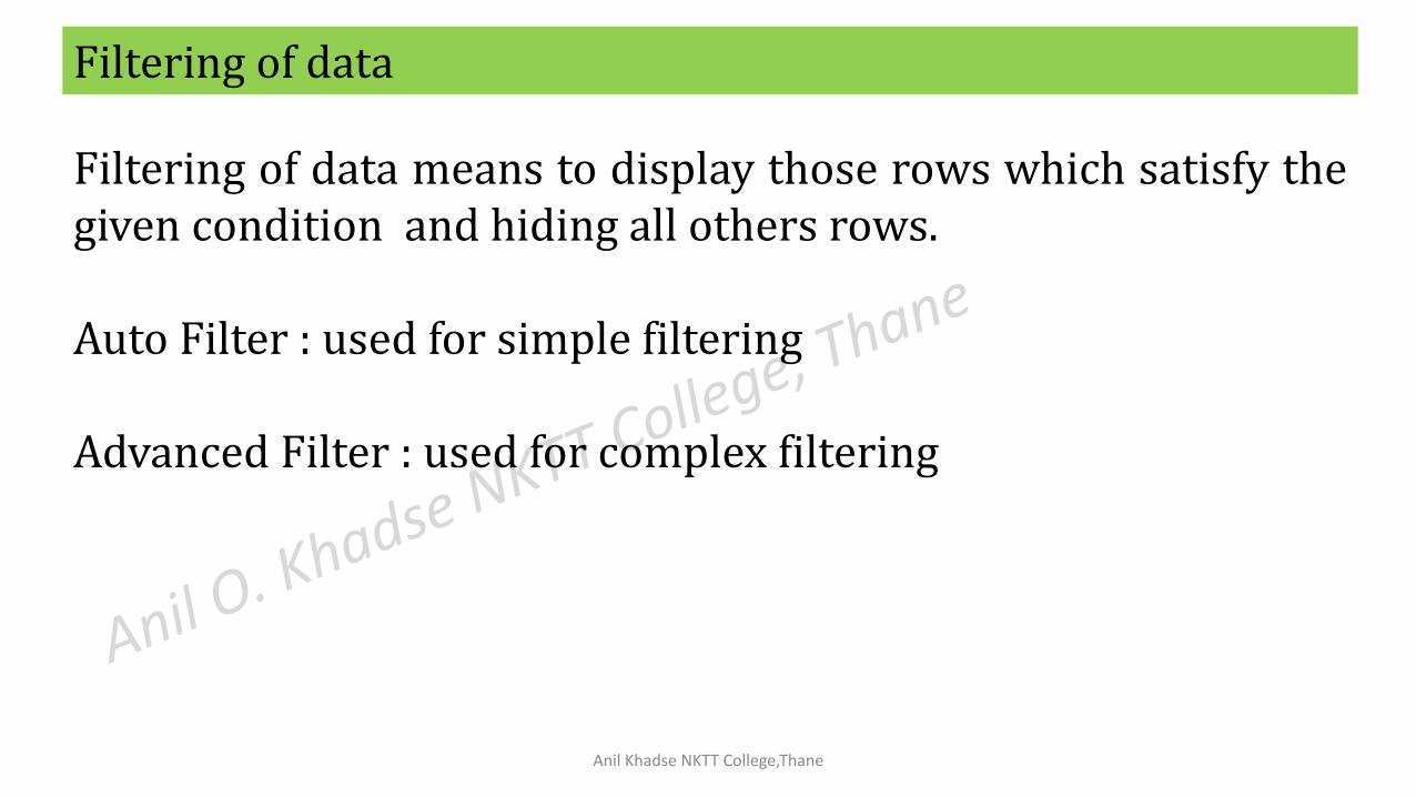
Filtering of data
Filtering of data means to display those rows which satisfy thegiven condition and hiding all others rows.
Auto Filter : used for simple filtering
Advanced Filter : used for complex filtering
Anil Khadse NKTT College,Thane
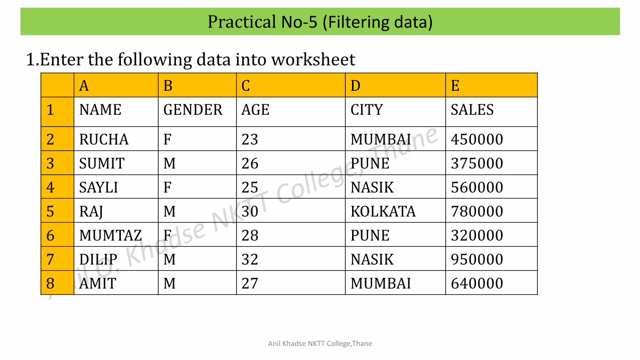
Practical No-5 (Filtering data)
1.Enter the following data into worksheet
A B C D E
1 NAME GENDER AGE CITY SALES
2 RUCHA F 23 MUMBAI 450000
3 SUMIT M 26 PUNE 375000
4 SAYLI F 25 NASIK 560000
5 RAJ M 30 KOLKATA 780000
6 MUMTAZ F 28 PUNE 320000
7 DILIP M 32 NASIK 950000
8 AMIT M 27 MUMBAI 640000
Anil Khadse NKTT College,Thane
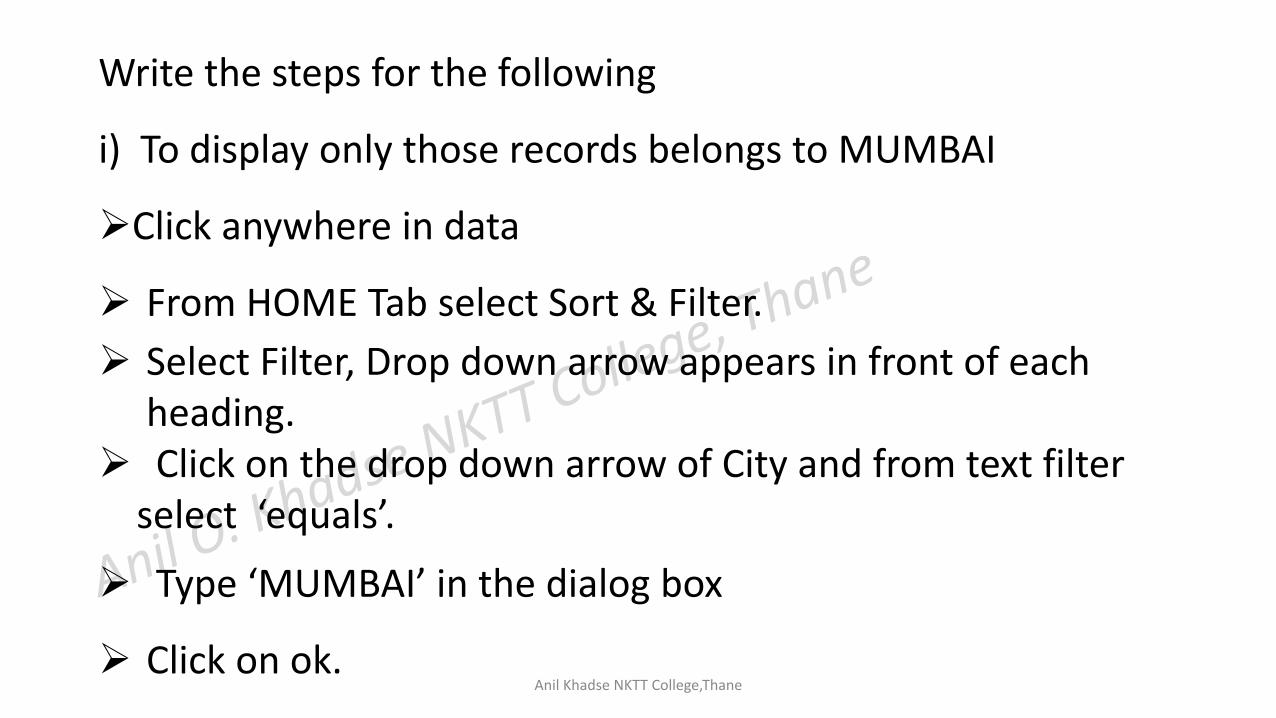
Write the steps for the following
i) To display only those records belongs to MUMBAI
Click anywhere in data
From HOME Tab select Sort & Filter.
Select Filter, Drop down arrow appears in front of each heading.
Click on the drop down arrow of City and from text filter select ‘equals’.
Type ‘MUMBAI’ in the dialog box
Click on ok.
Anil Khadse NKTT College,Thane
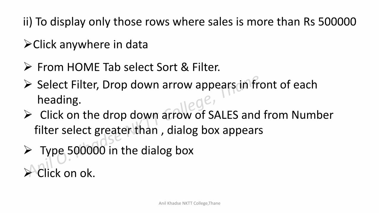
ii) To display only those rows where sales is more than Rs 500000
Click anywhere in data
From HOME Tab select Sort & Filter.
Select Filter, Drop down arrow appears in front of each heading.
Click on the drop down arrow of SALES and from Number filter select greater than , dialog box appears
Type 500000 in the dialog box
Click on ok.
Anil Khadse NKTT College,Thane
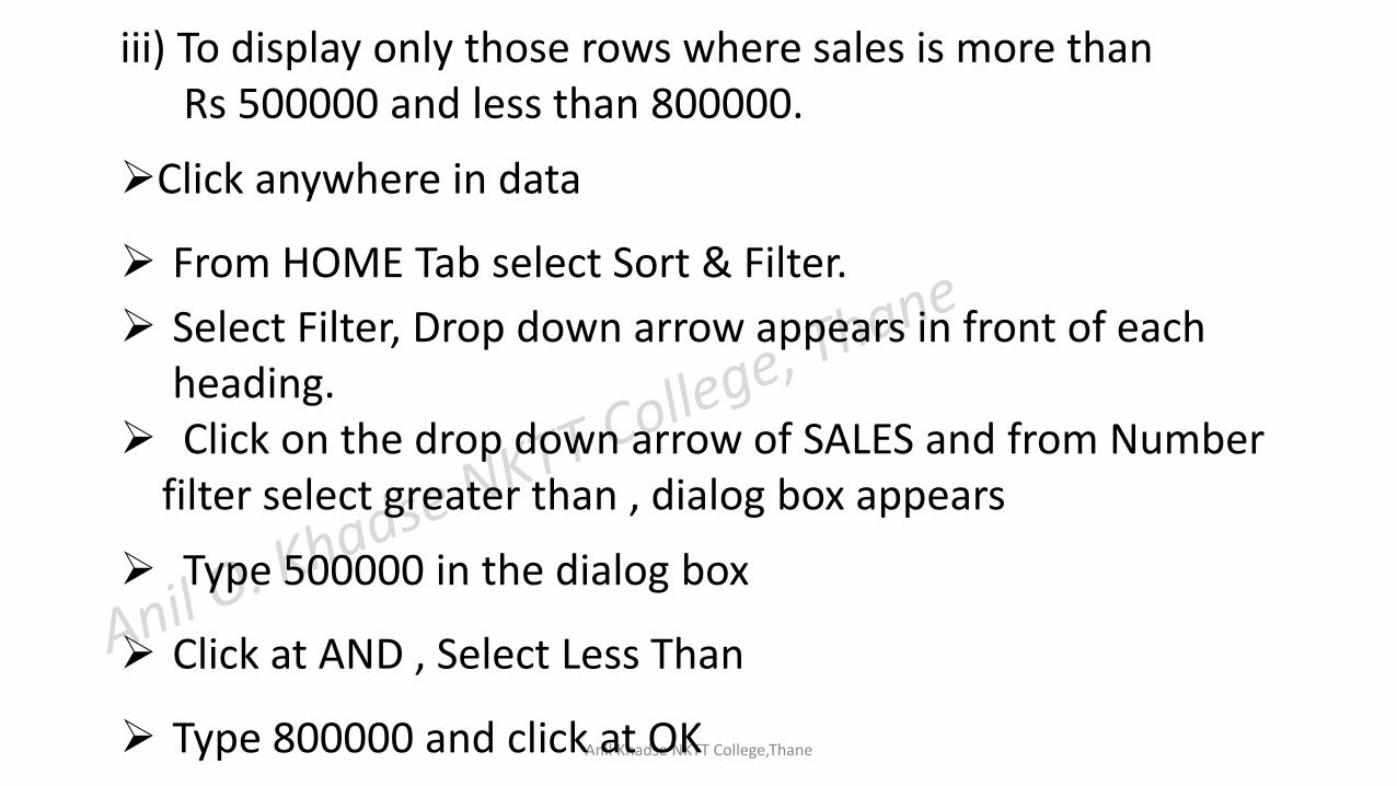
iii) To display only those rows where sales is more thanRs 500000 and less than 800000.
Click anywhere in data
From HOME Tab select Sort & Filter.
Select Filter, Drop down arrow appears in front of each heading.
Click on the drop down arrow of SALES and from Number filter select greater than , dialog box appears
Type 500000 in the dialog box
Click at AND , Select Less Than
Type 800000 and click at OK

Anil Khadse NKTT College,Thane
iv) To display only those records whose name begins with R Click anywhere in data
From HOME Tab select Sort & Filter.
Select Filter, Drop down arrow appears in front of each heading.
Click on the drop down arrow of NAME and from Text filter select begins with , dialog box appears
Type R in the dialog box
Click at OK
End of Practical - 5
Anil Khadse NKTT College,Thane
What If Analysis
Scenario Manager: Create different groups of values or scenario and can be switch between them.Used in budgeting to determine how change in values.It is available in DATA Tab Under What If Analysis
Goal Seek: It is used to find the single unknown value using the known valuesIt is available in DATA Tab Under What If Analysis
Anil Khadse NKTT College,Thane
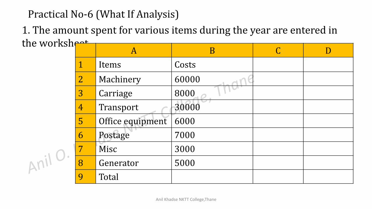
Practical No-6 (What If Analysis)
1. The amount spent for various items during the year are entered in the worksheet
A B C D
1 Items Costs
2 Machinery 60000
3 Carriage 8000
4 Transport 30000
5 Office equipment 6000
6 Postage 7000
7 Misc 3000
8 Generator 5000
9 Total
Anil Khadse NKTT College,Thane
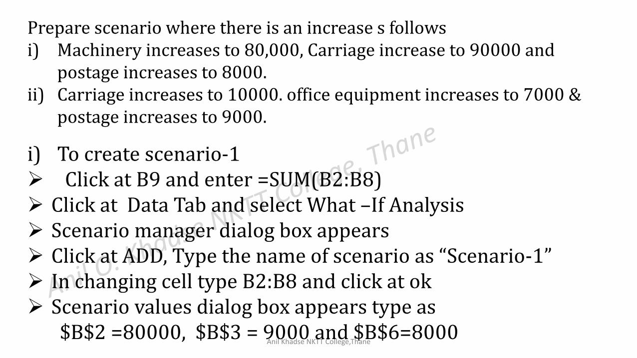
Prepare scenario where there is an increase s followsi) Machinery increases to 80,000, Carriage increase to 90000 and
postage increases to 8000.ii) Carriage increases to 10000. office equipment increases to 7000 &
postage increases to 9000.
i) To create scenario-1 Click at B9 and enter =SUM(B2:B8) Click at Data Tab and select What –If Analysis Scenario manager dialog box appears Click at ADD, Type the name of scenario as “Scenario-1” In changing cell type B2:B8 and click at ok Scenario values dialog box appears type as
$B$2 =80000, $B$3 = 9000 and $B$6=8000
Anil Khadse NKTT College,Thane
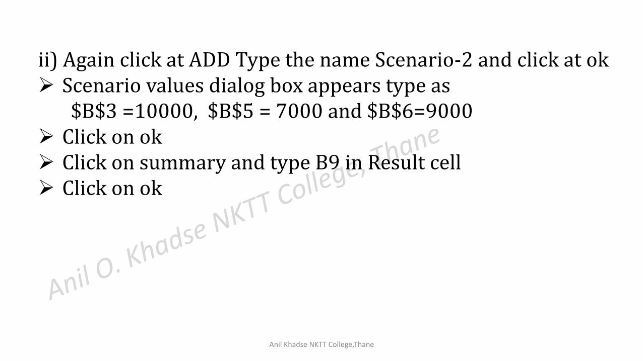
ii) Again click at ADD Type the name Scenario-2 and click at ok Scenario values dialog box appears type as
$B$3 =10000, $B$5 = 7000 and $B$6=9000 Click on ok Click on summary and type B9 in Result cell Click on ok
Anil Khadse NKTT College,Thane
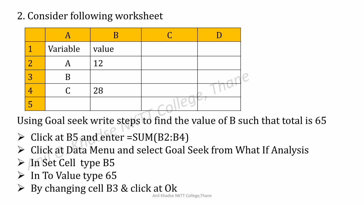
A B C D
1 Variable value
2 A 12
3 B
4 C 28
5
2. Consider following worksheet
Using Goal seek write steps to find the value of B such that total is 65
Click at B5 and enter =SUM(B2:B4) Click at Data Menu and select Goal Seek from What If Analysis In Set Cell type B5 In To Value type 65 By changing cell B3 & click at Ok
Anil Khadse NKTT College,Thane
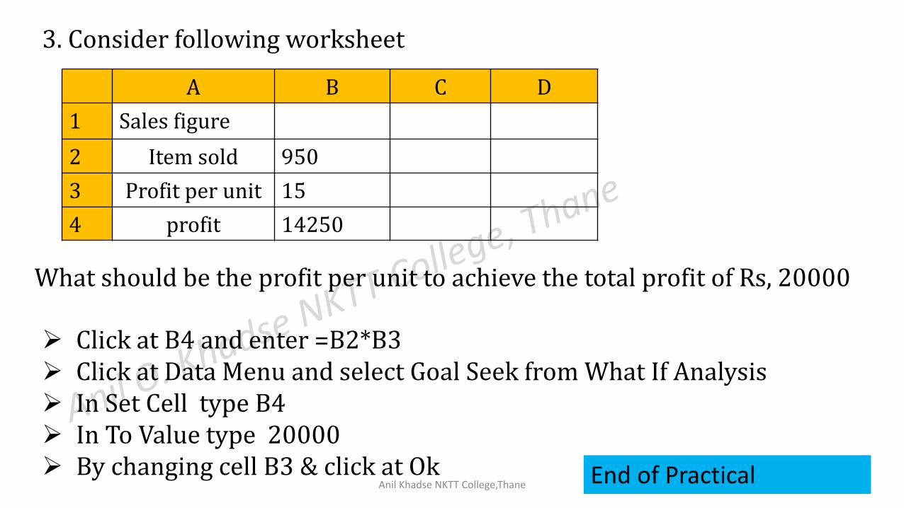
A B C D
1 Sales figure
2 Item sold 950
3 Profit per unit 15
4 profit 14250
3. Consider following worksheet
What should be the profit per unit to achieve the total profit of Rs, 20000
Click at B4 and enter =B2*B3 Click at Data Menu and select Goal Seek from What If Analysis In Set Cell type B4 In To Value type 20000 By changing cell B3 & click at Ok End of Practical
Anil Khadse NKTT College,Thane
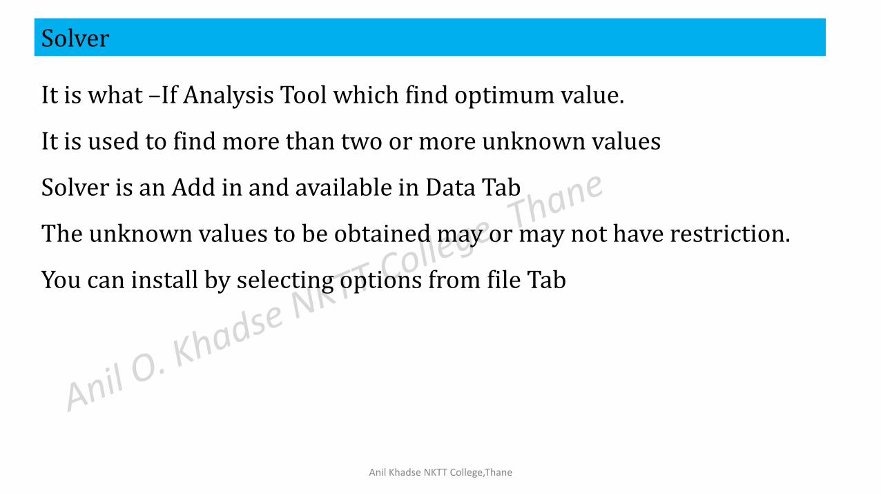
Solver
It is what –If Analysis Tool which find optimum value.
It is used to find more than two or more unknown values
Solver is an Add in and available in Data Tab
The unknown values to be obtained may or may not have restriction.
You can install by selecting options from file Tab
Anil Khadse NKTT College,Thane
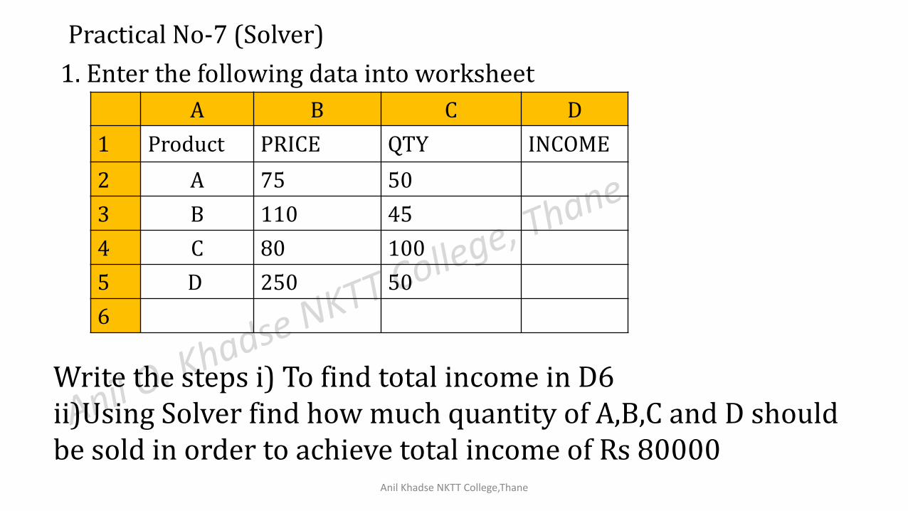
Practical No-7 (Solver)
1. Enter the following data into worksheet
A B C D
1 Product PRICE QTY INCOME
2 A 75 50
3 B 110 45
4 C 80 100
5 D 250 50
6
Write the steps i) To find total income in D6ii)Using Solver find how much quantity of A,B,C and D should be sold in order to achieve total income of Rs 80000
Anil Khadse NKTT College,Thane
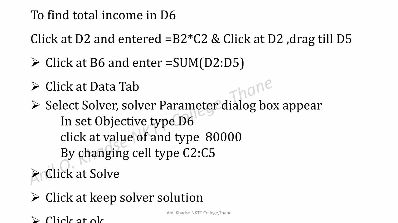
To find total income in D6
Click at D2 and entered =B2*C2 & Click at D2 ,drag till D5
Click at B6 and enter =SUM(D2:D5)
Click at Data Tab
Select Solver, solver Parameter dialog box appearIn set Objective type D6click at value of and type 80000By changing cell type C2:C5
Click at Solve
Click at keep solver solution
Click at ok
Anil Khadse NKTT College,Thane
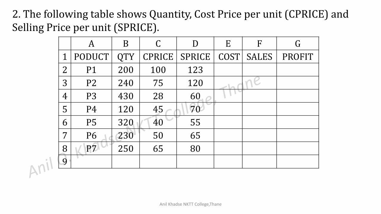
2. The following table shows Quantity, Cost Price per unit (CPRICE) and Selling Price per unit (SPRICE).
A B C D E F G
1 PODUCT QTY CPRICE SPRICE COST SALES PROFIT
2 P1 200 100 123
3 P2 240 75 120
4 P3 430 28 60
5 P4 120 45 70
6 P5 320 40 55
7 P6 230 50 65
8 P7 250 65 80
9
Anil Khadse NKTT College,Thane
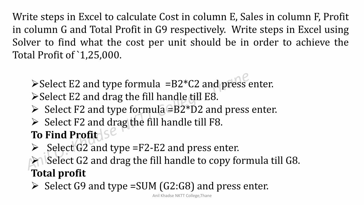
Write steps in Excel to calculate Cost in column E, Sales in column F, Profitin column G and Total Profit in G9 respectively. Write steps in Excel usingSolver to find what the cost per unit should be in order to achieve theTotal Profit of `1,25,000.
Select E2 and type formula =B2*C2 and press enter.Select E2 and drag the fill handle till E8. Select F2 and type formula =B2*D2 and press enter. Select F2 and drag the fill handle till F8.To Find Profit Select G2 and type =F2-E2 and press enter. Select G2 and drag the fill handle to copy formula till G8.Total profit Select G9 and type =SUM (G2:G8) and press enter.
Anil Khadse NKTT College,Thane
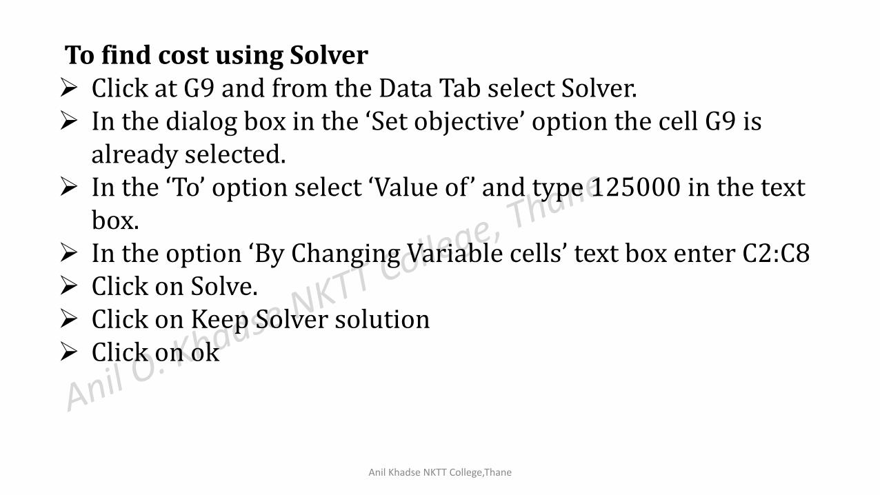
To find cost using Solver Click at G9 and from the Data Tab select Solver. In the dialog box in the ‘Set objective’ option the cell G9 is
already selected. In the ‘To’ option select ‘Value of’ and type 125000 in the text
box. In the option ‘By Changing Variable cells’ text box enter C2:C8 Click on Solve. Click on Keep Solver solution Click on ok
Anil Khadse NKTT College,Thane
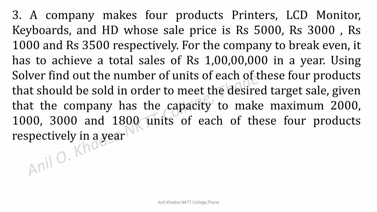
3. A company makes four products Printers, LCD Monitor,Keyboards, and HD whose sale price is Rs 5000, Rs 3000 , Rs1000 and Rs 3500 respectively. For the company to break even, ithas to achieve a total sales of Rs 1,00,00,000 in a year. UsingSolver find out the number of units of each of these four productsthat should be sold in order to meet the desired target sale, giventhat the company has the capacity to make maximum 2000,1000, 3000 and 1800 units of each of these four productsrespectively in a year
Anil Khadse NKTT College,Thane
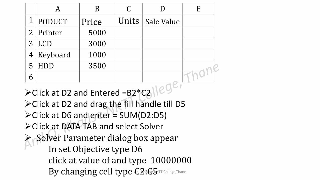
A B C D E
1 PODUCT Price Units Sale Value
2 Printer 5000
3 LCD 3000
4 Keyboard 1000
5 HDD 3500
6
Click at D2 and Entered =B2*C2Click at D2 and drag the fill handle till D5Click at D6 and enter = SUM(D2:D5)Click at DATA TAB and select Solver Solver Parameter dialog box appear
In set Objective type D6click at value of and type 10000000By changing cell type C2:C5

Anil Khadse NKTT College,Thane
Click at ADD to add constraints
C2<=2000, Click at ADD
C3<=1000, Click at ADD
C4<=3000, Click at ADD
C5<=1800
Click on ok
Click on solve
Click at keep solver solution
Click at ok
Anil Khadse NKTT College,Thane
Charts
Bar DiagramColum DiagramPie ChartLine
Anil Khadse NKTT College,Thane
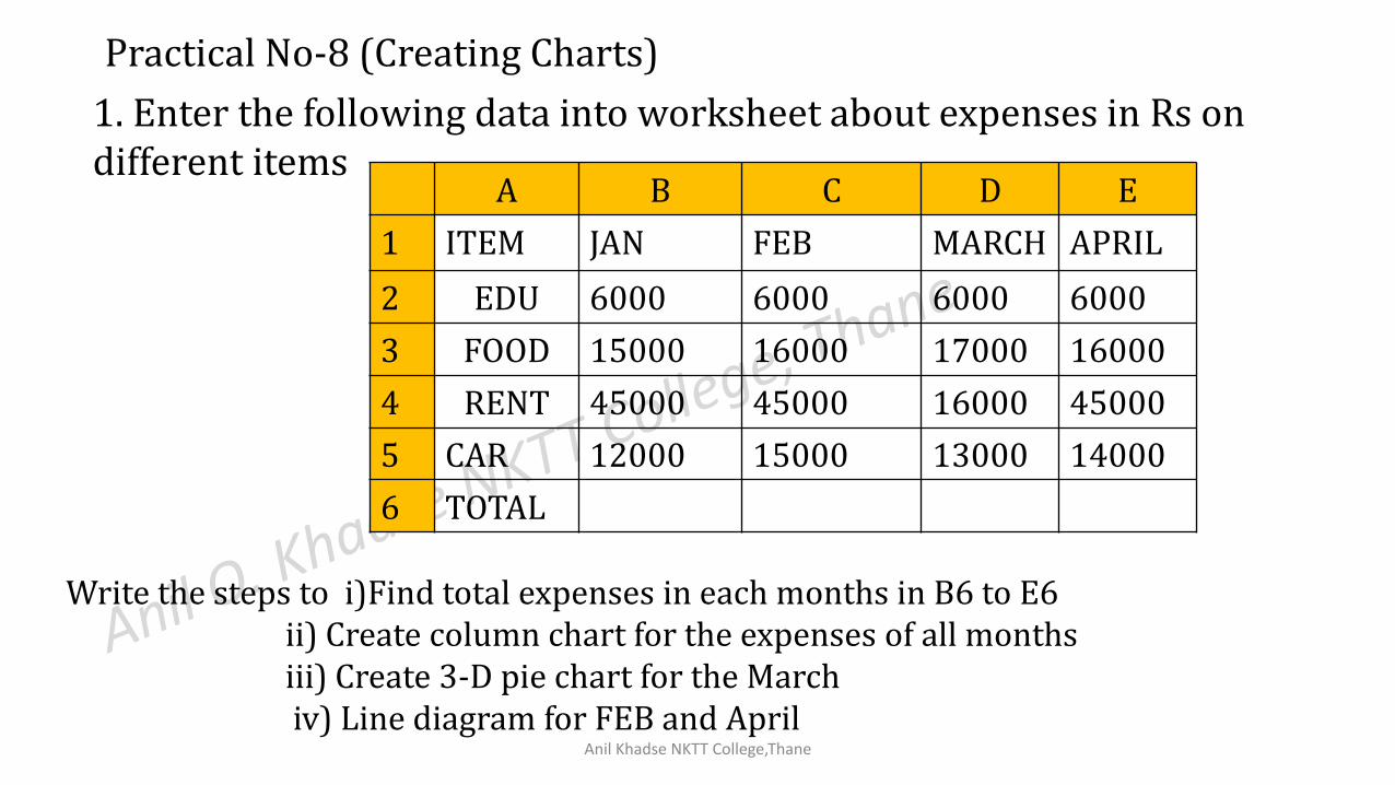
Practical No-8 (Creating Charts)
1. Enter the following data into worksheet about expenses in Rs on different items
A B C D E
1 ITEM JAN FEB MARCH APRIL
2 EDU 6000 6000 6000 6000
3 FOOD 15000 16000 17000 16000
4 RENT 45000 45000 16000 45000
5 CAR 12000 15000 13000 14000
6 TOTAL
Write the steps to i)Find total expenses in each months in B6 to E6ii) Create column chart for the expenses of all monthsiii) Create 3-D pie chart for the Marchiv) Line diagram for FEB and April
Anil Khadse NKTT College,Thane
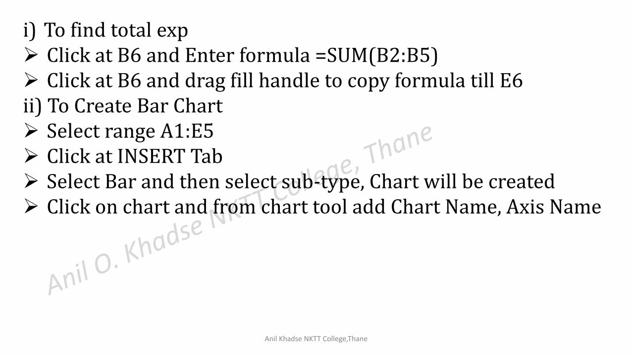
i) To find total exp Click at B6 and Enter formula =SUM(B2:B5) Click at B6 and drag fill handle to copy formula till E6ii) To Create Bar Chart Select range A1:E5 Click at INSERT Tab Select Bar and then select sub-type, Chart will be created Click on chart and from chart tool add Chart Name, Axis Name
Anil Khadse NKTT College,Thane
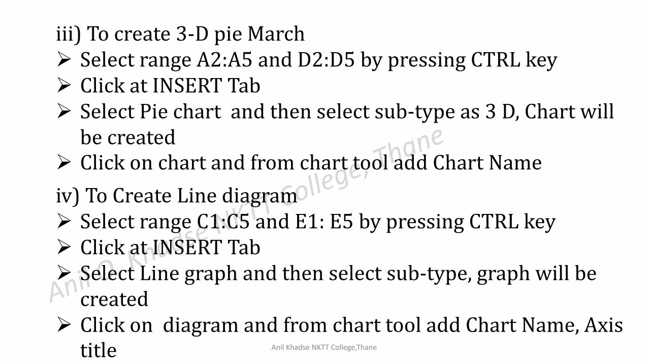
iv) To Create Line diagram Select range C1:C5 and E1: E5 by pressing CTRL key Click at INSERT Tab Select Line graph and then select sub-type, graph will be
created Click on diagram and from chart tool add Chart Name, Axis
title
iii) To create 3-D pie March Select range A2:A5 and D2:D5 by pressing CTRL key Click at INSERT Tab Select Pie chart and then select sub-type as 3 D, Chart will
be created Click on chart and from chart tool add Chart Name

Anil Khadse NKTT College,Thane
Recommended