1
RIETI Discussion Paper Series 17-E-081
Revised in November 2017
Uncertainty over Production Forecasts: An Empirical Analysis Using Monthly
Firm Survey Data
Masayuki Morikawa
Abstract
This study, using monthly micro data on firms’ forecasted and realized production
quantities, presents new evidence of the uncertainty of production forecasts. We make a
number of novel findings that contribute to the literature on this topic. Forecast errors
are heterogeneous among individual manufacturers, while firms operating in the
information and communications technology-related industries, firms producing
investment goods, and smaller firms exhibit greater forecast uncertainty. Moreover,
forecast uncertainty is greater in the contractionary phases of the business cycle and the
uncertainty measures calculated from the micro data are able to predict macroeconomic
fluctuations. Finally, the forecast uncertainty of Japanese manufacturing firms is
associated with overseas policy uncertainty in addition to Japan’s own economic policy
uncertainty.
Keywords: production, uncertainty, forecast error, manufacturing, volatility
Research Institute of Economy, Trade and Industry (RIETI). 1-3-1 Kasumigaseki, Chiyoda-ku, Tokyo 100-8901, Japan. E-mail address: [email protected]; [email protected]. Tel.: +81-3-3501-1362. I would like to thank Haruhiko Ando, Yasuo Goto, Seiichiro Inoue, Arata Ito, Keisuke Kondo, Atsushi Nakajima, Norio Nakazawa, Yukiko Saito, Makoto Yano, Hiroyuki Yoshiya, and the seminar participants at RIETI for their valuable comments and suggestions. Any errors are my own. I am grateful to the Ministry of Economy, Trade and Industry for providing the micro data of the Survey of Production Forecast used in this study. This research is supported by JSPS Grants-in-Aid for Scientific Research (26285063, 26590043).

2
JEL Classification: D84, E32, E66, L60
RIETI Discussion Papers Series aims at widely disseminating research results in the form of professional papers, thereby stimulating lively discussion. The views expressed in the papers are solely those of the author(s), and do not present those of the Research Institute of Economy, Trade and Industry.

3
Uncertainty over Production Forecasts: An Empirical Analysis Using Monthly
Firm Survey Data
1. Introduction
Uncertainty and its impacts on economic activities attract attention from policy
practitioners and economic researchers. Uncertainty, which arises from financial crises,
unexpected policy developments in major countries following changes of political
power, and natural disasters, among other factors, negatively affects firm behavior over
the course of the economy, particularly impacting on long-term investments including
innovation and recruitment (see Carruth et al., 2000 and Bloom, 2014 for surveys).
Since uncertainty is subjective in nature and not directly observable from statistical
data, various proxy variables have been proposed to capture the uncertainty faced by
economic agents.1 Representative uncertainty measures include the (1) volatility of
stock prices (Bloom et al., 2007; Bloom, 2009), (2) cross-sectional disagreement of
forecasts by professional economists (Driver and Moreton, 1991; Dovern et al., 2012),
(3) unexplained portion of macroeconomic variables derived from econometric models
(Jurado et al., 2015), (4) ex post forecast errors in firms’ business outlook (Bachmann et
al., 2013; Arslan et al., 2015; Morikawa, 2016a), (5) survey-based firms’ subjective
uncertainty (Guiso and Parigi, 1999; Bontempi, 2016; Morikawa, 2016b), and (6)
frequency of newspaper articles on policy uncertainty (Baker et al., 2016).
The measure of uncertainty adopted in this study is the ex post errors in the
production forecasts of manufacturing firms. Although firms’ forecast errors have been
used as proxy of uncertainty in the literature, empirical studies have generally depended
on the qualitative outlook of business conditions (e.g., improving, unchanging, or
deteriorating) available from business surveys (Bachmann et al., 2013; Arslan et al.,
1 The ideal measure to capture the uncertainty faced by economic agents is the point forecast and its probability distribution of individual firms or households (Pesaran and Weale, 2006); however, such data for individual companies or households are rarely available.
4
2015; Morikawa, 2016a). By contrast, this study uses quantitative data on ex ante
production forecasts and ex post realized production at the firm- and product-levels
taken from a monthly survey of Japanese manufacturers conducted by the Ministry of
Economy, Trade and Industry (METI), namely the Survey of Production Forecast (SPF).
A small number of studies analyze quantitative forecast errors at the firm-level. For
example, Bachmann and Elstner (2015), using quarterly survey data on manufacturing
firms in Germany (i.e., the IFO Business Climate Survey), quantify and analyze
production errors. However, since production quantities are not directly available from
the survey data, they construct quantitative expectation errors for firms’ production
growth from the expectation of capacity utilization rates based on several assumptions,
such as production capacity remaining constant. Bachmann et al. (2017) present a
quantitative analysis of a firm-level investment expectation error termed investment
surprise for a 40-year panel of German manufacturing firms (i.e., the IFO Investment
Survey). Although the availability of a long panel is an advantage, the investment data
used in their study have only an annual frequency.
By contrast, the SPF captures the cyclical movements of Japanese manufacturers’
production on a monthly basis. The survey specifically asks firms for their production
forecasts for the next month, estimated production for the current month, and realized
production for the previous month. Because no analyses of forecast errors using
monthly frequency quantitative firm- and product-level production have thus far been
carried out, this study contributes to the literature on uncertainty in two main ways.2
First, when only data on qualitative forecasts and realizations are available, unexpected
improvements (or deteriorations) in business conditions are treated equally. However, in
practice, the economic impacts of forecast errors of 5% and 50%, for example, are very
different. Second, adopting firm- and product-level micro data enables us to analyze not
only the time-series properties of uncertainty but also its cross-sectional heterogeneity
by industry or product type. While production uncertainty is naturally heterogeneous
2 Bachmann and Elstner (2015), who analyze firms’ forecast errors using micro data from German manufacturers, state that “ideally, researchers would need high-frequency quantitative expectation and realization data on firm-specific variables,” but that “such information is not available for under-yearly frequencies and for long time horizons in any business survey we know of.”
5
and rest heavily on the characteristics of the industries or products in question, such an
analysis has been hampered by data limitations.
By using these novel data, we make seven important findings about production
uncertainty at the firm- and product-levels. First, forecast errors differ by firms. Indeed,
even when realized production at the aggregate-level is corrected downward from the
forecast (i.e., overpredicted), many firms’ realized production amounts are corrected
upward from their forecasted amounts (i.e., underpredicted). Second, while realized
production tends to be slightly less (about 2% on average) than forecasted production,
the average absolute forecast error is larger than 10%. Third, firms operating in
information and communications technology (ICT)-related industries, firms producing
investment goods, and smaller firms exhibit greater production uncertainty. Fourth, the
higher the volatility of actual production in the recent past, the greater forecast
uncertainty will be, suggesting that past production volatility can be used as a proxy of
uncertainty. Fifth, forecast uncertainty heightens in contractionary phases of the
business cycle. In particular, production uncertainty rises at the time of large exogenous
shocks such as the global financial crisis (2008–2009) and Great East Japan Earthquake
(2011). Sixth, the uncertainty measures calculated from the firm-level micro data are
able to predict macroeconomic fluctuations that cannot be detected from the measures
constructed from publicly available aggregated data, indicating the value of firm-level
production forecast data. Seventh, the production uncertainty of Japanese manufacturing
firms is associated with overseas policy uncertainty in addition to Japan’s own
economic policy uncertainty (EPU).
The remainder of this paper is structured as follows. Section 2 explains the data used
in this study, the procedure for calculating the forecast errors and uncertainty measures,
and the method of analysis. Section 3 reports the results, including (1) descriptive
observations on the time-series movements of forecast uncertainty; (2) differences in
uncertainty by industry, product type, and firm size; (3) the relationship between
forecast uncertainty and production volatility; (4) the cyclical characteristics of forecast
uncertainty; and (5) the relationship between the production uncertainty and EPU
indices constructed from the frequency of newspaper articles. Section 4 concludes,
6
presenting the policy implications, limitations of the study, and issues to be addressed in
future work.
2. Data and Method of Analysis
A. The SPF
This study uses monthly firm- and product-level micro data taken from the SPF from
January 2006 to March 2015. The SPF collects information on firms’ forecasts of the
following month’s production quantity, estimated production quantity for the current
month, and realized production quantity for the previous month. For example, the
February survey asks for the production forecast for March, estimated production for
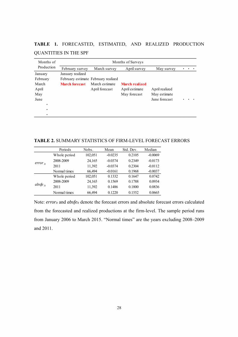
February, and realized production for January. Table 1 summarizes the time structure of
the survey. The survey is carried out at the end of each month and the deadline for
reporting is the 10th of the following month.3
The survey data are used to construct the Indices of Production Forecast (IPF), which
show the forecasted manufacturing production relative to the base year (currently
2010).4 IPF is an important macroeconomic statistic for judging business cycle phases.
In particular, the “realization ratio,” namely the gap between the realized production of
the current month’s survey and estimated production of the previous month’s survey,
and the “amendment ratio,” the gap between the estimated production of the current
month’s survey and forecasted production of the previous month’s survey, are regarded
as useful measures for judging the turning points of business cycles. For example,
unexpected negative (positive) figures of these ratios may signal that the business cycle
is approaching its peak (trough).
3 The details of the survey including the survey form are available at the website of the METI (http://www.meti.go.jp/statistics/tyo/yosoku/). 4 The IPF is published monthly at the same time as the release of the Indices of Industrial Production (IIP), which are similar to the Industrial Production and Capacity Utilization (constructed by the Federal Reserve Bank) in the United States.
7
The SPF surveys 195 manufacturing products and approximately 700 firms. Sample
firms are chosen on a product-by-product basis to cover approximately 80% of the
domestic production of each product, as determined from the annual Current Survey of
Production (conducted by the METI).5 The resampling of firms is conducted every five
years to retain the 80% coverage of the production of each product. However, about
60% of these firms were surveyed throughout the sample period used in this study.
Moreover, as forecasted and realized monthly productions of more than 90% of the
surveyed products are expressed as quantities (rather than as monetary values) such as
tonnage or the number of products, most production data are real figures unaffected by
price changes. For example, the unit of quantities of iron and steel products and
chemicals is expressed in tonnage, while that of vehicles and household electronic
appliances is expressed in the number of products manufactured.6
The SPF classifies industries into (1) iron and steel, (2) non-ferrous metals, (3)
fabricated metals, (4) general machinery, (5) electronic parts and devices, (6) electrical
machinery, (7) information and communication electronics equipment, (8) transport
equipment, (9) chemicals, (10) pulp, paper, and paper products, and (11) other
manufacturing. In addition, the products are, based on their major use, categorized into
(1) capital goods, (2) construction goods, (3) durable consumer goods, (4) non-durable
consumer goods, (5) producer goods for manufacturing, and (6) producer goods for
non-manufacturing. Unfortunately, firm characteristics other than industry and product
category, such as the number of employees and firm age, are not included in the SPF.7
In this study, we define the production forecast error as the gap between realized
production and forecasted production. For example, the difference between the
forecasted production for March in the February survey and the realized production for
March in the April survey is the forecast error. The size of the forecast error can be
5 The Current Survey of Production is similar to the Annual Survey of Manufacturers in the United States. 6 Since the units of quantity measure differs by product, it is not possible to aggregate production quantity across different products. 7 As the micro data of the SPF is highly confidential, the names of the firms surveyed are unavailable to researchers. Therefore, it is impossible to link the data with other firm surveys to obtain firm characteristics.
8
interpreted as the degree of production forecast uncertainty at the time of the survey
(February, in this case).
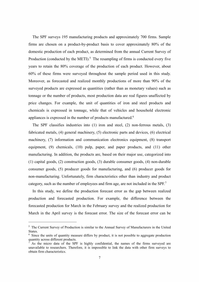
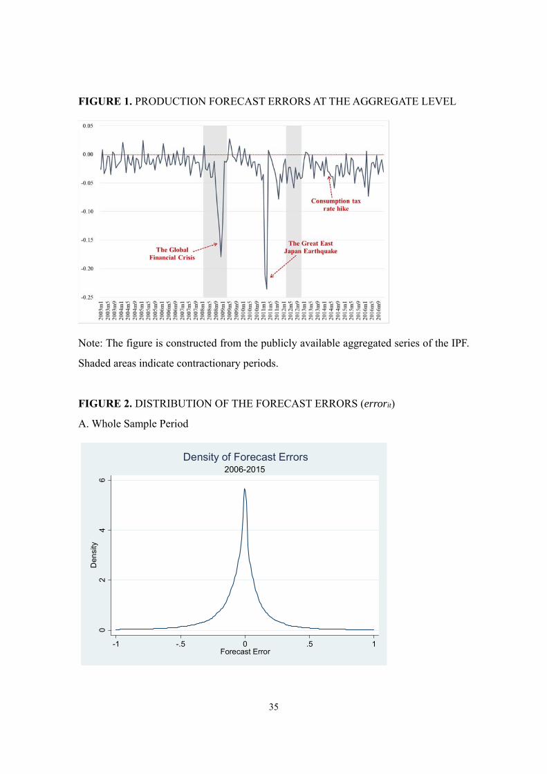
It is possible to calculate the forecast errors at the aggregate-level from the published
series of the IPF. Figure 1 depicts the movements of the forecast errors for the whole
manufacturing sector,8 showing two huge negative surprises (forecasted production >
realized production) during the global financial crisis (2008–2009) and Great East Japan
Earthquake (2011) periods. In normal times, small negative surprises are frequent, but
positive surprises (forecasted production < realized production) can occur. The absolute
sizes of both positive and negative surprises proxy for the degree of macro-level
production uncertainty at the time of forecasting.
However, even when realized production underperforms forecasted production at the
aggregate-level, some firms underperform and other firms overperform (relative to their
forecasts) at the micro-level. In other words, there are large gross forecast errors behind
the relatively small net forecast errors.9 These aggregated net forecast errors conceal
the heterogeneous movements of individual firms. For example, when the
overperformed production amount is the same as the underperformed production
amount, the net forecast error (or production uncertainty) calculated from the aggregate
indices will be zero. However, it is natural to think that uncertainty is greater when large
positive and negative forecast errors co-exist than when both positive and negative
errors are small. It is for this reason that we use firm- and product-level micro data
derived from the SPF to present new empirical evidence on the production forecast
uncertainty of Japanese manufacturers.10
8 Data on aggregated IPF is available from the website of the METI (http://www.meti.go.jp/statistics/tyo/iip/). 9 Research using qualitative business survey data indicates that many positive and negative surprises co-exist at the firm-level, even when the forecast error at the aggregate level is small (Morikawa, 2016a). 10 Although the currently available data period is limited to about 10 years between January 2006 and March 2015, the total number of observations is more than 100,000. As the Survey of Production Forecast is regarded as containing highly confidential information about firms’ production forecast, more recent data are unavailable for researchers.
9
B. Method of Analysis
By using the data set explained above, we first calculate simple forecast errors at the
firm- and product-levels. The production quantity of firm i in month t (qit) is converted
into the logarithmic form and the difference between forecasted production (ln(E(qit)))
and realized production (ln(qit)) is defined as the “forecast error” of production (errorit),
which is the measure of production uncertainty at the firm- and product-levels adopted
in this study:
errorit = ln(qit) - ln(E(qit)) (1)
A positive errorit indicates that the firm’s production forecast was underpredicted (or
a positive surprise), whereas a negative errorit means overprediction (or a negative
surprise). To avoid the confounding effects of extremely large positive/negative values,
we remove the observations when the absolute value of errorit exceeds unity as
outliers. 11 Because the figures are expressed in logarithmic form, when either
forecasted or realized production is zero, the forecast error is treated as a missing
value.12
Next, we calculate the absolute forecast error (absfeit) as the absolute value of errorit,
which is an alternative measure of production uncertainty at the firm- and
product-levels:
absfeit = | errorit | (2)
Based upon these micro-level production uncertainty measures, we then construct
time-series data on aggregate production uncertainty. Specifically, following studies that
11 In total, 1,922 observations (1.8%) are dropped. As the standard deviation of errorit before removing outliers is 0.324, removing observations of errorit that exceed unity is similar to removing observations that are either three standard deviations larger or smaller than the sample mean. 12 Zero production (about 4% of the observations) sometimes occurs in cases when a factory either goes into periodic maintenance or stops operation following an accident.
10
have used qualitative business survey data (Bachmann et al., 2013; Morikawa, 2016a),
we define the (1) mean absolute forecast error (denoted as MEANABSFEt) and (2)
forecast error dispersion (denoted as FEDISPt) as measures of production uncertainty at
time t. MEANABSFEt is the means of the individual absolute forecast errors (absfeit) at
time t. FEDISPt is the cross-sectional dispersion of the individual forecast errors
(errorit) at time t calculated as the standard deviation. We calculate these uncertainty
measures (MEANABSFEt and FEDISPt) by industry and product type in addition to for
the whole manufacturing sector to detect differences at a more fine-grained level.
These two aggregated measures serve as our proxies of production uncertainty even
though they are conceptually different. For example, when all firms overpredicted their
production in the next month (downward correction ex post) by the same magnitude,
MEANABSFEt takes a positive value, whereas FEDISPt is zero by definition. However,
according to studies using qualitative business survey data (Bachmann et al., 2013;
Morikawa, 2016a), MEANABSFEt and FEDISPt generally exhibit similar time-series
movements.
By using these firm-level and aggregated measures of production uncertainty, we first
document their headline time-series properties and the differences by industry and
product type. We then analyze the differences by producer size by dividing the sample
into large and small producers, as the qualitative forecast errors of large firms are less
than those of small firms (Bachmann and Elstner, 2015; Morikawa, 2016a). Because the
SPF does not contain information about firm characteristics, as noted above, we divide
the sample into large and small producers based upon the mean production quantity of
each producer during the sample period. Specifically, the production quantity of firm i
(qi) averaged in the sample period is calculated, and a large (small) producer is defined
as a firm whose production quantity is larger (smaller) than the mean quantity ( ) of the
product. We then test the statistical differences of errorit and absfeit by producer size.
Next, we analyze the relationships between production volatility and the production
uncertainty measures at the firm-level. While past volatility is frequently used as a
proxy of economic uncertainty, it does not necessarily represent the future uncertainty
faced by firms. Our main interest here is whether greater volatility in the past is
11
positively associated with greater forecast uncertainty in the future. In this analysis, we
thus measure a firm’s production volatility as the coefficient of variation (standard
deviation divided by the mean) of production in the 12 months before the time of
forecasting.
Uncertainty measures have a countercyclical property in that uncertainty heightens
during recessions and declines during booms (Bloom, 2014; Jurado et al., 2015). To
verify this property at the firm-level, we divide the sample period into expansionary and
contractionary phases and test the statistical differences of errorit and absfeit by these
cyclical phases.13 In addition, we analyze the relationships between the aggregated
uncertainty measures (MEANABSFEt and FEDISPt) and macroeconomic fluctuations,
such as the lead–lag relationships. Although it is natural to use GDP as a representative
macroeconomic time series, GDP data are available only at a quarterly frequency.
Therefore, we use the monthly Indices of All Industry Activity (IAA) to analyze the
relationships with the measures of production forecast uncertainty.14
Finally, we analyze the relationship between the production uncertainty measures
calculated from the SPF and the EPU indices constructed from the frequency of
newspaper articles (Baker et al., 2016). The global EPU index (EPU–Global) and index
for the United States (EPU–US), in addition to the EPU index for Japan (EPU–Japan),
are available on a monthly basis. 15 We analyze the correlations and lead–lag
relationships of our measure of forecast uncertainty with the EPU indices.
3. Results
A. Forecast Errors at the Firm-Level
13 In Japan, the reference dates of the business cycle are discussed in the Investigation Committee for Business Cycle Indicators and determined by the Economic and Social Research Institute of the Cabinet Office. 14 The IAA is constructed by weight-averaging the indices of various industries with the added value weights of the base year. The IAA data are available at the website of METI (http://www.meti.go.jp/statistics/tyo/zenkatu/). 15 The outline of the global EPU index is explained by Davis (2016).
12
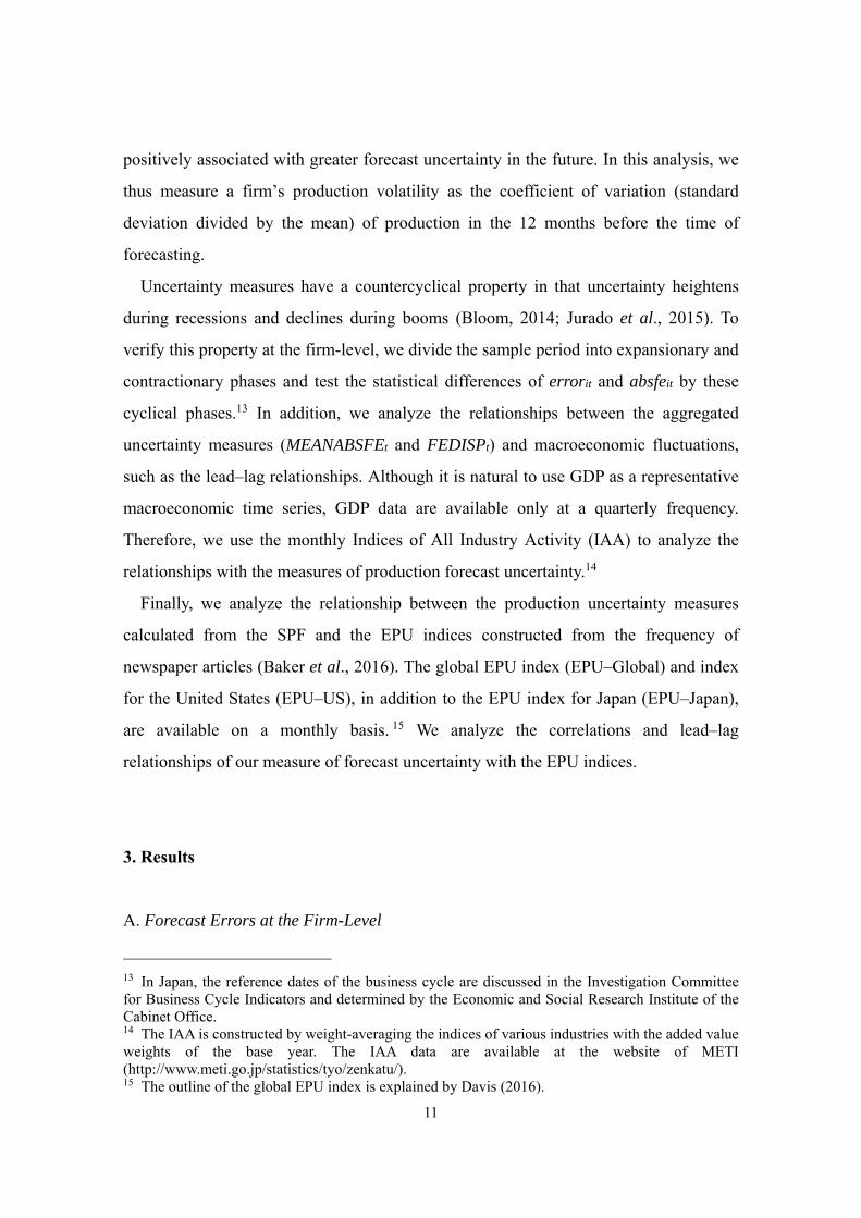
Table 2 reports the summary statistics of the forecast errors (errorit) and absolute
forecast errors (absfeit) throughout the sample period (2006–2015). The means of errorit
and absfeit are -0.024 and 0.133, respectively. During the sample period, realized
production falls short of the forecast by 2.4% and the absolute forecast error is more
than 10% on average. However, the medians are -0.007 and 0.074, respectively, which
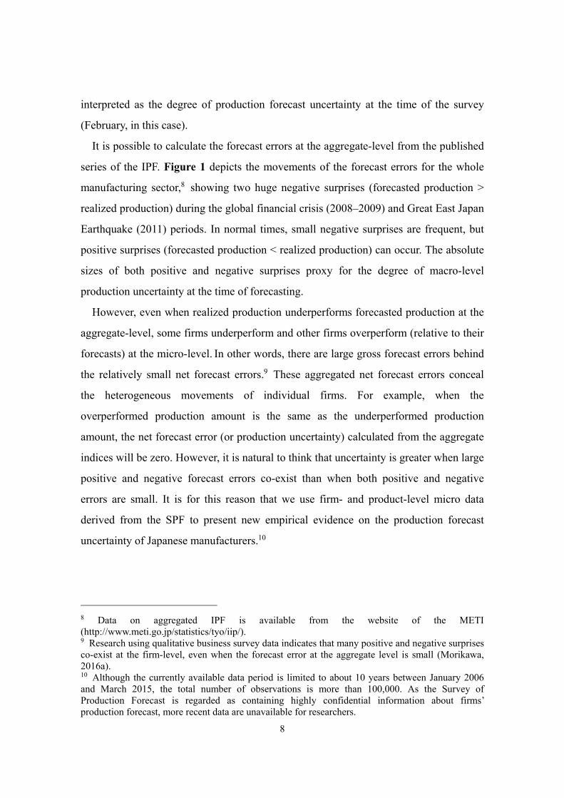
are smaller in absolute terms than the mean figures. Figure 2-A illustrates the
distribution of the forecast errors (errorit). Although those calculated from the IPF tend
to show downward corrections (see Figure 1), the firm-level forecast errors are
concentrated around zero and distributed evenly on both the positive and the negative
sides. However, at the same time, the tails of the distribution are long, indicating that
firms sometimes experience either large positive or large negative forecast errors.
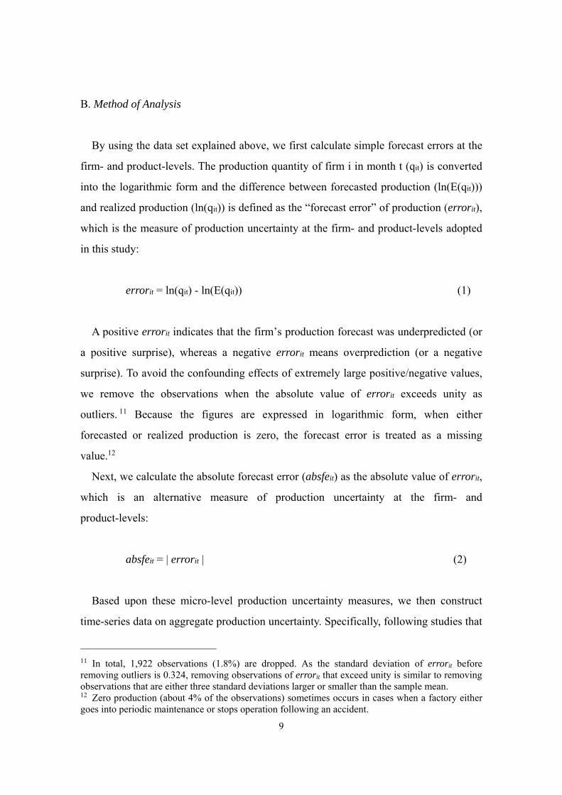
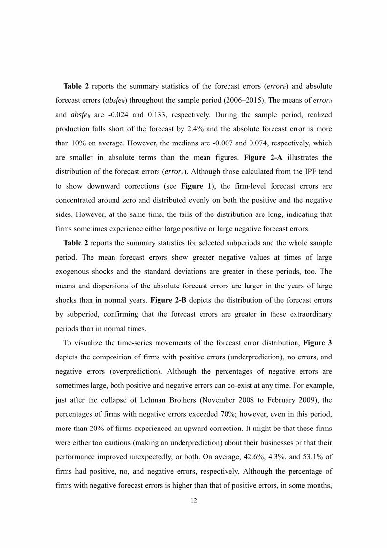
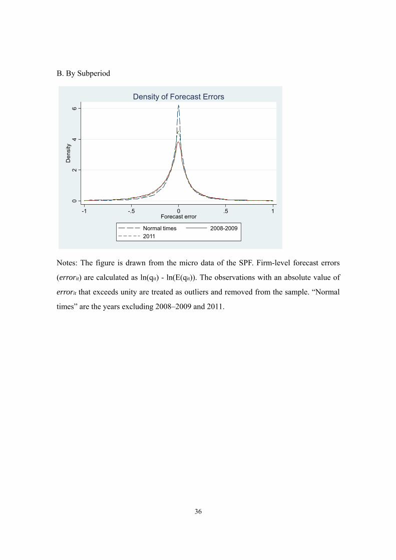
Table 2 reports the summary statistics for selected subperiods and the whole sample
period. The mean forecast errors show greater negative values at times of large
exogenous shocks and the standard deviations are greater in these periods, too. The
means and dispersions of the absolute forecast errors are larger in the years of large
shocks than in normal years. Figure 2-B depicts the distribution of the forecast errors
by subperiod, confirming that the forecast errors are greater in these extraordinary
periods than in normal times.
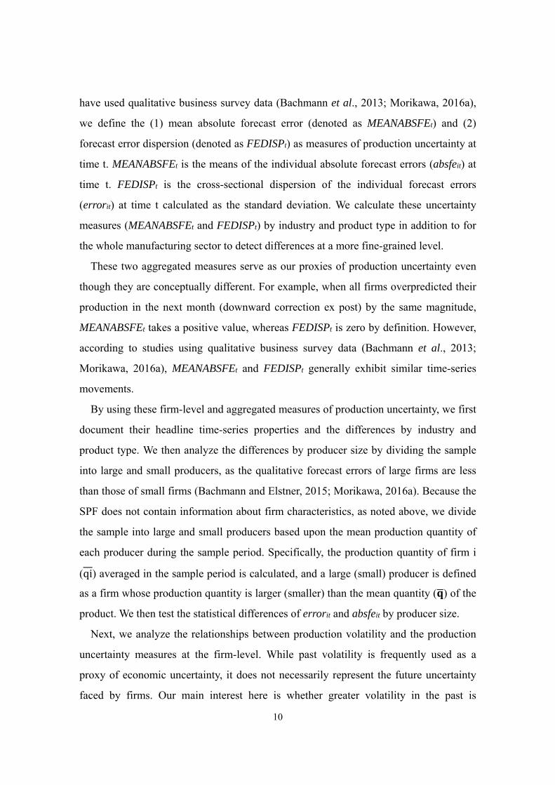
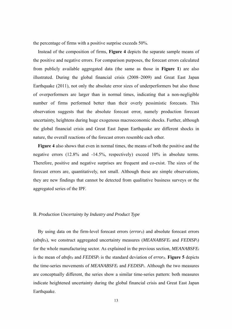
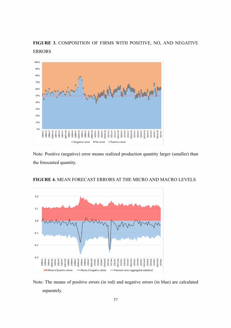
To visualize the time-series movements of the forecast error distribution, Figure 3
depicts the composition of firms with positive errors (underprediction), no errors, and
negative errors (overprediction). Although the percentages of negative errors are
sometimes large, both positive and negative errors can co-exist at any time. For example,
just after the collapse of Lehman Brothers (November 2008 to February 2009), the
percentages of firms with negative errors exceeded 70%; however, even in this period,
more than 20% of firms experienced an upward correction. It might be that these firms
were either too cautious (making an underprediction) about their businesses or that their
performance improved unexpectedly, or both. On average, 42.6%, 4.3%, and 53.1% of
firms had positive, no, and negative errors, respectively. Although the percentage of
firms with negative forecast errors is higher than that of positive errors, in some months,
13
the percentage of firms with a positive surprise exceeds 50%.
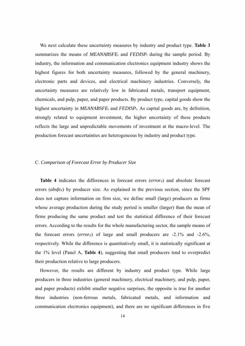
Instead of the composition of firms, Figure 4 depicts the separate sample means of
the positive and negative errors. For comparison purposes, the forecast errors calculated
from publicly available aggregated data (the same as those in Figure 1) are also
illustrated. During the global financial crisis (2008–2009) and Great East Japan
Earthquake (2011), not only the absolute error sizes of underperformers but also those
of overperformers are larger than in normal times, indicating that a non-negligible
number of firms performed better than their overly pessimistic forecasts. This
observation suggests that the absolute forecast error, namely production forecast
uncertainty, heightens during huge exogenous macroeconomic shocks. Further, although
the global financial crisis and Great East Japan Earthquake are different shocks in
nature, the overall reactions of the forecast errors resemble each other.
Figure 4 also shows that even in normal times, the means of both the positive and the
negative errors (12.8% and -14.5%, respectively) exceed 10% in absolute terms.
Therefore, positive and negative surprises are frequent and co-exist. The sizes of the
forecast errors are, quantitatively, not small. Although these are simple observations,
they are new findings that cannot be detected from qualitative business surveys or the
aggregated series of the IPF.
B. Production Uncertainty by Industry and Product Type
By using data on the firm-level forecast errors (errorit) and absolute forecast errors
(absfeit), we construct aggregated uncertainty measures (MEANABSFEt and FEDISPt)
for the whole manufacturing sector. As explained in the previous section, MEANABSFEt
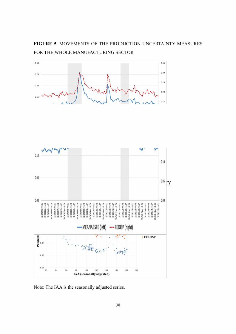
is the mean of absfeit and FEDISPt is the standard deviation of errorit. Figure 5 depicts
the time-series movements of MEANABSFEt and FEDISPt. Although the two measures
are conceptually different, the series show a similar time-series pattern: both measures
indicate heightened uncertainty during the global financial crisis and Great East Japan
Earthquake.
14
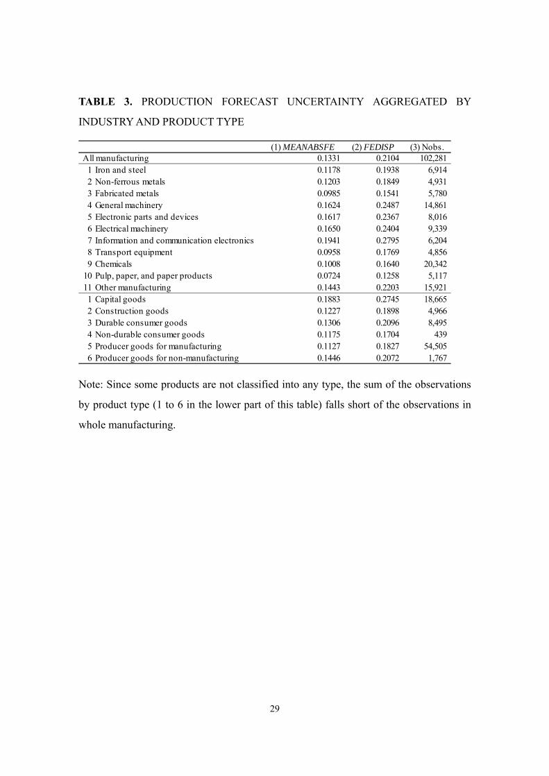
We next calculate these uncertainty measures by industry and product type. Table 3
summarizes the means of MEANABSFEt and FEDISPt during the sample period. By
industry, the information and communication electronics equipment industry shows the
highest figures for both uncertainty measures, followed by the general machinery,
electronic parts and devices, and electrical machinery industries. Conversely, the
uncertainty measures are relatively low in fabricated metals, transport equipment,
chemicals, and pulp, paper, and paper products. By product type, capital goods show the
highest uncertainty in MEANABSFEt and FEDISPt. As capital goods are, by definition,
strongly related to equipment investment, the higher uncertainty of these products
reflects the large and unpredictable movements of investment at the macro-level. The
production forecast uncertainties are heterogeneous by industry and product type.
C. Comparison of Forecast Error by Producer Size
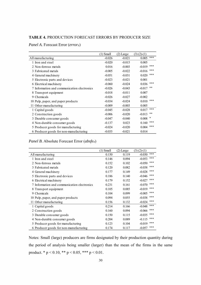
Table 4 indicates the differences in forecast errors (errorit) and absolute forecast
errors (absfeit) by producer size. As explained in the previous section, since the SPF
does not capture information on firm size, we define small (large) producers as firms
whose average production during the study period is smaller (larger) than the mean of
firms producing the same product and test the statistical difference of their forecast
errors. According to the results for the whole manufacturing sector, the sample means of
the forecast errors (errorit) of large and small producers are -2.1% and -2.6%,
respectively. While the difference is quantitatively small, it is statistically significant at
the 1% level (Panel A, Table 4), suggesting that small producers tend to overpredict
their production relative to large producers.
However, the results are different by industry and product type. While large
producers in three industries (general machinery, electrical machinery, and pulp, paper,
and paper products) exhibit smaller negative surprises, the opposite is true for another
three industries (non-ferrous metals, fabricated metals, and information and
communication electronics equipment), and there are no significant differences in five
15
industries (iron and steel, electronic parts and devices, transport equipment, chemicals,
and other manufacturing). By product type, large producers exhibit smaller negative
surprises in four product categories (capital goods, durable consumer goods,
non-durable consumer goods, and producer goods for manufacturing), but the result for
construction goods is the opposite. Small producers’ tendency to overpredict is not
common across either industry or product type.
By contrast, the results for the absolute forecast errors (absfeit) indicate clearly that
the forecasts of smaller producers are less accurate (Panel B, Table 4). In the whole
manufacturing sector, the figures for large and small producers are 11.9% and 15.0%,
respectively. These differences are statistically significant at the 1% level in every
industry and product category. By industry, the gaps by producer size are remarkable
among firms in the information and communication electronics equipment, iron and
steel, non-ferrous metals, and electronic parts and devices industries.
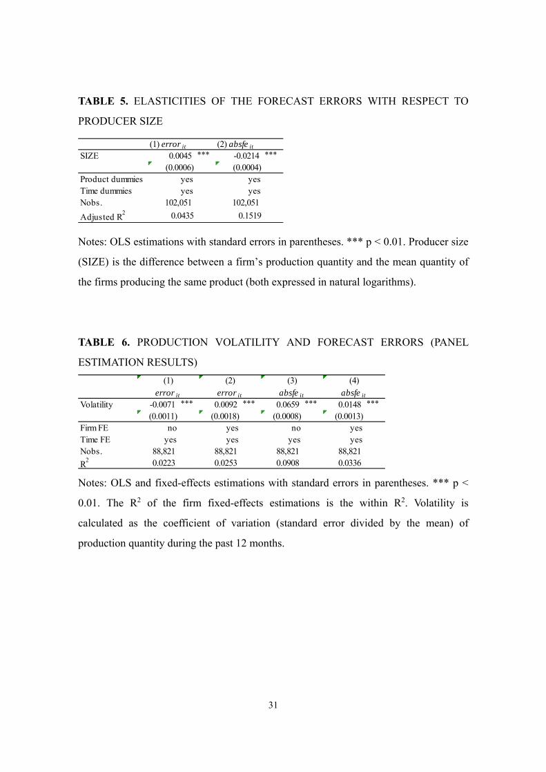
Instead of dividing the sample into large and small subsamples, we run a simple
regression, where producer size (the log of the production quantity relative to the
product mean) is used as a continuous explanatory variable and the forecast errors and
absolute forecast errors are used as the dependent variables. Product dummies and time
(month) dummies are also used as control variables. In the regressions, as both producer
size and forecast errors are expressed in logarithmic form, the estimated coefficients for
producer size can be interpreted as the elasticity of forecast errors with respect to
producer size. The finding that small producers tend to face greater production
uncertainty, or, in other words, that the forecasts of large producers are relatively
accurate, is confirmed from the regression analysis using the continuous producer size
variable (Table 5). The difference by size is pronounced in the case of using absolute
forecast errors as the dependent variable (column (2), Table 5), indicating that doubling
the size of a producer reduces the absolute forecast error by 1.5% on average.
Our inference is that the absolute forecast error (absfeit), which shows the accuracy of
the production forecast irrespective of the sign, is a better measure of uncertainty of the
production forecast than is the simple forecast error (errorit), which reflects optimism
and pessimism in addition to pure (non-directional) uncertainty. In short, the production
16
forecasts of large producers are either more accurate than those of small producers or
small producers face greater forecast uncertainty in their production. This result is
consistent with the findings of studies using quarterly qualitative business survey data
(Bachmann and Elstner, 2015; Morikawa, 2016a). Our interpretation of this result is that
the costs of gathering and processing information to make production forecasts are
somewhat fixed and that large producers strive to forecast accurately by investing in
such information activities.
D. Production Volatility and Forecast Errors
Table 6 reports the panel estimation results of the relationship between the volatility
of realized production and forecast error at the firm-level. In these regressions, the
dependent variables are the forecast errors (errorit) and absolute forecast errors (absfeit)
alternatively. The explanatory variable is production volatility over the past 12 months,
calculated as the coefficient of variation. Time fixed-effects are used to control for the
macroeconomic conditions common across firms. We conduct two estimation patterns
where firm fixed-effects are either included or omitted.
Columns (1) and (2) of Table 6 presents the regression results using the simple
forecast error (errorit) as the dependent variable. The coefficients of past production
volatility are negative and significant when firm fixed-effects are not included, meaning
that firms with more volatile production in the recent past tend to show greater negative
surprises (column (1)). However, the signs of the coefficients turn positive when firm
fixed-effects are included (column (2)), meaning that after accounting for unobservable
firm characteristics, greater volatility in recent past production is associated with a
larger positive surprise (or a smaller negative surprise) in the near future. This result
suggests that firms tend to make cautious production forecasts after experiencing large
production fluctuations, resulting in an underprediction.
When the absolute forecast error (absfeit) is used as the dependent variable, the
volatility coefficients are found to be positive and highly significant irrespective of the
17
inclusion of firm fixed-effects (columns (3) and (4), Table 6). The greater the
production volatility in the recent past, the more uncertain the forecasts of future
production will be. From the viewpoint of empirical research on uncertainty, this result
suggests that production volatility can be used as a practical proxy of uncertainty about
production in the near future.
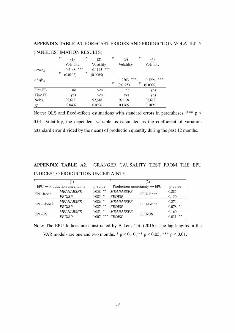
If we reverse the variables, namely using realized production volatility during the
future 12 months as the dependent variable and either errorit or absfeit as the
explanatory variable, the estimated coefficients for errorit are negative and those for
absfeit are positive, with both statistically significant at the 1% level (Appendix Table
A1). These results hold irrespective of including firm fixed-effects, indicating that
greater forecast uncertainty is associated with volatile production in the near future.
E. Business Cycles and Production Uncertainty
Many studies of macroeconomic uncertainty have indicated that uncertainty rises in
recessions and falls in booms (Bloom, 2014). In this subsection, we first examine the
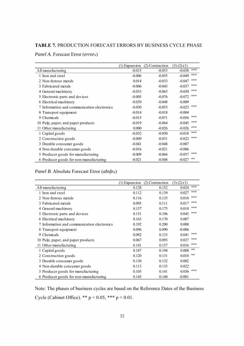
differences in the firm-level forecast errors by phases of the business cycle. Table 7
summarizes the comparisons by the business cycle phases with statistical significance.
According to the results of the forecast errors (errorit) for the whole manufacturing
sector, the means of negative surprises in expansionary and contractionary phases are
-1.5% and -5.3%, respectively (Panel A, Table 7). Obviously, the statistical difference is
highly significant. By industry, the negative surprise (or overprediction) is larger in
contractionary phases in every industry, and the differences are statistically significant
in nine of 11 industries, with the exception of the electrical machinery and transport
equipment industries. While the mean size of overprediction (downward correction)
stands out in industries such as electrical machinery, general machinery, and
information and communication electronics equipment, the differences by cyclical
phases are large in electronic parts and devices and chemicals.
By product type, a significantly larger negative surprise in contractionary phases is
18
observed in capital goods, construction goods, producer goods for manufacturing, and
production goods for non-manufacturing. The difference by cyclical phases is prominent
in firms/products belonging to producer goods for manufacturing: the means of negative
surprises in the expansionary and contractionary phases are -0.9% and -6.6%,
respectively. As most products classified in electronic parts and devices and chemicals
industries belong to producer goods, the results by industry and product type are
consistent.
Panel B of Table 7 compares the absolute forecast errors (absfeit). For the whole
manufacturing sector, these errors in the expansionary and contractionary phases are
12.8% and 15.2%, respectively. While the difference is not large, it is statistically
significant at the 1% level. By industry, the absolute forecast errors in the contractionary
phase are larger than those in the expansionary phase for the majority of industries, with
the exception of transport equipment, and the differences are statistically significant in
eight industries. By product type, larger absolute forecast errors are found in capital
goods, construction goods, and producer goods for manufacturing. The production
forecasts of these product categories become inaccurate in contractionary phases.
As the above observations are based on the dichotomic division of cyclical phases,
the magnitude of the strength or weakness of overall economic activity is not considered.
To quantify the degree of macroeconomic conditions, we compare the relationships
between the measures of production uncertainty (MEANABSFEt and FEDISPt) and the
IAA. The horizontal axis in Figure 6 is the seasonally adjusted IAA and the vertical
axis is the production uncertainty measures for the whole manufacturing sector. As can
be seen, uncertainty for both MEANABSFEt and FEDISPt is lower when
macroeconomic activity level is higher and vice versa. The correlation coefficients with
the IAA are -0.574 for MEANABSFEt and -0.672 for FEDISPt.
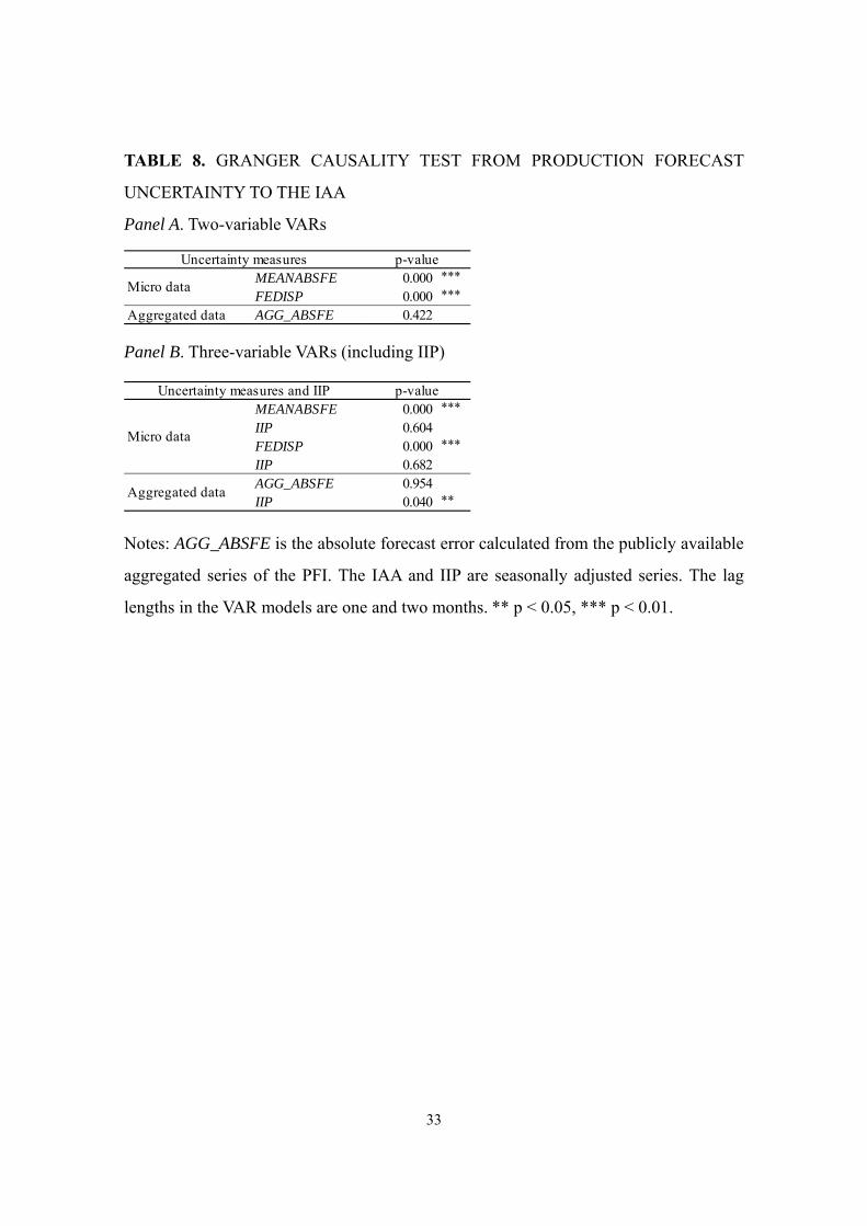
While this figure plots the simultaneous relationships between the IAA and
production uncertainty measures, there may be lead–lag relationships. In this respect,
we estimate simple vector autoregressive (VAR) models to detect the Granger causality
running from the uncertainty measures to IAA. The lag lengths in these VAR models are

19
one and two months.16 We find that both uncertainty measures (MEANABSFEt and
FEDISPt) have significant Granger causality to the IAA at the 1% level (Panel A, Table
8). On the contrary, the reverse causality from the IAA to the uncertainty measures is
insignificant for both MEANABSFEt and FEDISPt (p-values are 0.825 and 0.359; not
reported in the table).
However, these results may reflect the lead–lag relationship between the economic
activity of the manufacturing sector and the whole economy (IAA). To check this
possibility, we conduct VAR models with three variables, including the IIP as an
additional variable.17 Even if we include the IIP in the model, both uncertainty
measures still Granger cause the IAA (Panel B, Table 8). On the contrary, we do not
find significant causality running from the IIP to IAA. The results of these exercises
suggest that macroeconomic activity tends to decline shortly after production
uncertainty calculated from the firm-level forecast errors rises.
On the contrary, when we use the absolute forecast error of production calculated
from the publicly available aggregated IPF (denoted as AGG_ABSFEt), we cannot
detect Granger causality from this measure to the IAA (see the lower parts of Panels A
and B, Table 8). This result indicates that the uncertainty measures calculated from the
firm- and product-level micro data contain valuable information for judging the
development of business cycles, which is not obtainable from the publicly available
aggregated series of the IPF. Indeed, when we estimate the same models excluding the
years of the global financial crisis (2008–2009) and Great East Japan Earthquake (2011),
we still detect that MEANABSFEt and FEDISPt Granger cause the IAA, but that
AGG_ABSFEt does not.
Furthermore, we estimate the VAR models of the same specifications by using the
monthly Indices of Business Conditions constructed by the Cabinet Office as an
alternative measure of macroeconomic activity. The results are consistent with those
obtained by using the IAA. MEANABSFEt, and FEDISPt Granger cause these indices
16 Even when longer lags (e.g., three months and four months) are added into the VAR models, the results are essentially unchanged. 17 Seasonally adjusted series of the IIP are used.
20
(p-values are 0.000), whereas AGG_ABSFEt does not show Granger causality (p-value
is 0.693). In summary, the results that the uncertainty measures calculated from
firm-level data have Granger causality to macroeconomic activity and that the causality
cannot be detected from the measure derived from publicly available aggregated data
are robust.
F. Production Forecast Uncertainty and EPU
In this subsection, we present evidence of the relationships between our measures of
production forecast uncertainty (MEANABSFE and FEDISP) and the EPU indices. The
newspaper-based EPU indices developed by Baker et al. (2016) have frequently been
used in recent empirical studies of policy uncertainty.18 Currently, the monthly EPU
indices for the United States, the European Union, Japan, and other countries are
available to researchers. More recently, the Global EPU index (EPU–Global), which is
the weighted average of the EPU indices of individual countries, has also been released.
As we are interested in the extent to which domestic and overseas policy uncertainties
affect Japanese manufacturing firms, this study uses the EPU index for Japan (EPU–
Japan) as well as EPU–Global or, alternatively, the index for the United States (EPU–
US).19 We adopt EPU–US as an alternative to EPU–Global because the latter, by
construction, contains information about EPU–Japan, which may not represent pure
overseas policy uncertainty.
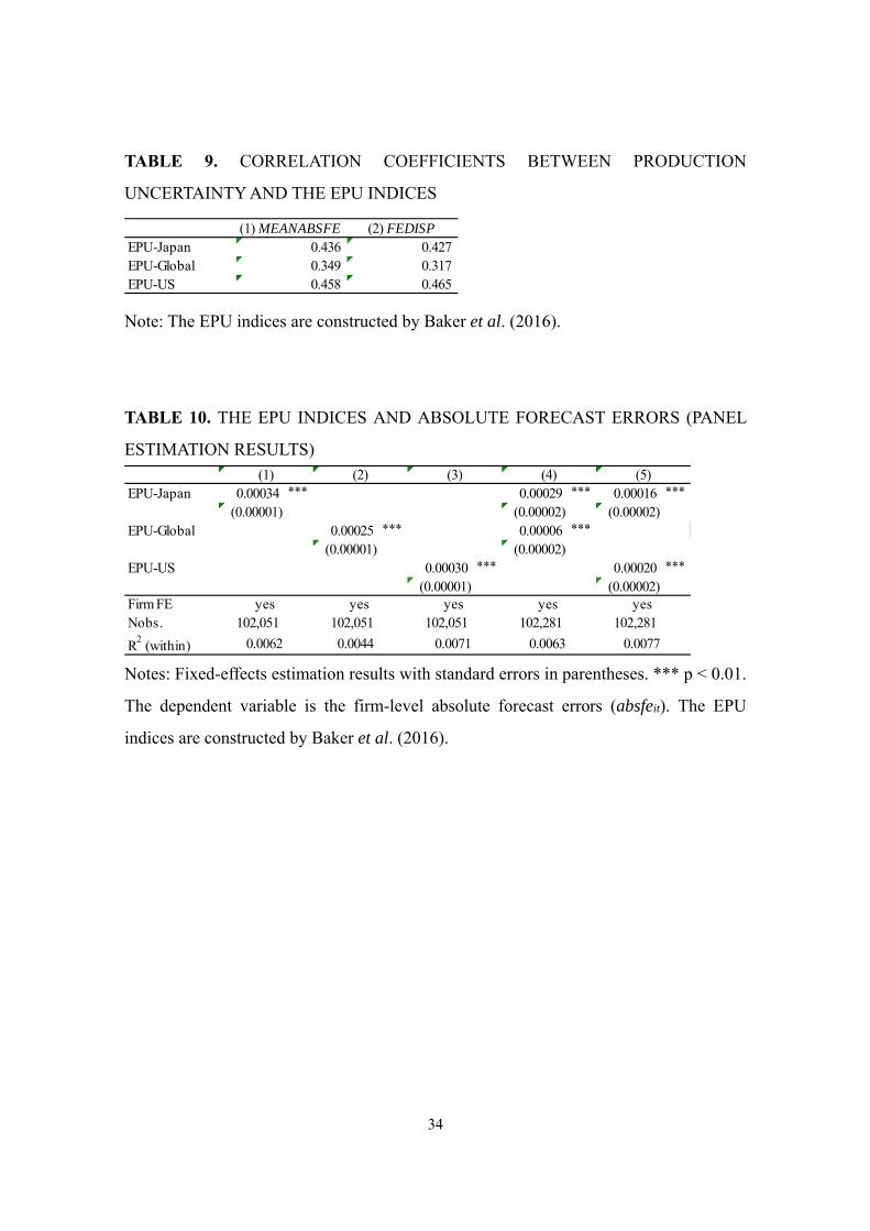
Table 9 presents the correlation coefficients between our measures of production
uncertainty and the EPU indices. MEANABSFE and FEDISP have positive correlations
with both EPU–Japan and EPU–Global, indicating that production uncertainty is
18 Recent studies using EPU indices include Bernal et al. (2016), Gulen and Ion (2016), Caggiano et al. (2017), and Meinen and Roehe (2017). 19 The data on EPU–Japan used in this study are the latest series at the time of writing; they were provided by Dr. Arata Ito, a co-author of Arbatli et al. (2017). The other series were downloaded from the Economic Policy Uncertainty website.
21
associated with uncertain policy developments.20 Unexpectedly, the correlations with
EPU–US are slightly stronger than those with EPU–Japan, possibly because the
production forecasts of Japanese manufacturing firms depend heavily on policy
developments in the United States. These observations are consistent with studies based
on firm surveys (Morikawa, 2016b, 2016c) that indicate that Japanese firms,
particularly manufacturing firms, are concerned about policy uncertainty related to
international trade.
Table 10 reports the results from a simple panel regression analysis, where the
absolute forecast error at the firm-level (absfeit) is treated as the dependent variable and
the EPU indices are used as explanatory variables. In these estimations, firm
fixed-effects are controlled for. When the policy uncertainty indices are included
separately, the coefficients for EPU–Japan, EPU–Global, and EPU–US are all positive
and significant at the 1% level and the sizes of the coefficients are similar (columns (1)–
(3)), suggesting that firms’ production forecasts become inaccurate when domestic and
overseas policy uncertainty heightens.
When EPU–Japan and EPU–Global are simultaneously used as the explanatory
variables, both coefficients are positive and statistically significant, whereas the size of
the coefficient for EPU–Japan is about five times greater than that for EPU–Global
(column (4)). As EPU–Global contains information about EPU–Japan, we re-estimate
by replacing EPU–Global with EPU–US (column (5)). Interestingly, in this specification,
the coefficient for EPU–US is slightly larger than that for EPU–Japan, confirming that
the accuracy of Japanese manufacturing firms’ production forecasts is heavily affected
by EPU in the United States. Even when we estimate the same models excluding the
years of the global financial crisis (2008–2009) and Great East Japan Earthquake (2011),
the sizes of the coefficients for the EPU indices reduced, but they are still statistically
significant.
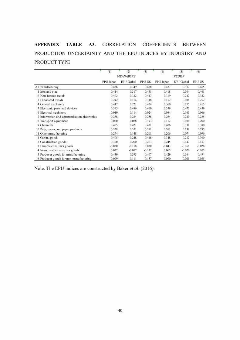
Finally, Appendix Table A3 reports the correlation coefficients with the EPU indices
20 When testing Granger causality between our measures of production uncertainty and the EPU Indices, EPU–Japan, EPU–Global, and EPU–US weakly Granger cause MEANABSFE and FEDISP (Appendix Table A2).
22
by industry and product type. Similar to the findings for the whole manufacturing sector,
the production uncertainties of most industries correlate with, in descending order,
EPU–US, EPU–Japan, and EPU–Global. However, the electronic parts and devices
industry is an important exception. In this industry, both MEANABSFE and FEDISP
have higher correlations with EPU–Global and EPU–US than with EPU–Japan.
Unexpectedly, the correlations of the production uncertainty of the transport equipment
industry with the EPU indices are generally low, possibly reflecting the accuracy of
production forecasts in this industry indicated before. By product type, the production
uncertainty of construction goods has higher correlations with EPU–Japan than the
overseas EPU indices, as expected from the domestic nature of this industry. On the
contrary, the production uncertainty of capital and producer goods for manufacturing
has the highest correlations with EPU–US.
To summarize, these results suggest that Japanese manufacturing firms, particularly
those producing parts, components, and materials, are involved in the deepening global
value chain. As a result, these firms’ production forecasts are affected by the
development of overseas policy uncertainty.
4. Conclusion
This study, using monthly micro data on Japanese manufacturing firms’ forecasted
and realized production taken from the SPF, presents new findings on the uncertainty of
production forecasts. The major results and the implications of the first empirical study
adopting monthly-frequency quantitative production forecast data at the firm- and
product-levels are as follows. First, forecast errors at the firm-level often differ from
those derived from publicly available aggregated data. Even when realized production at
the aggregate level is downward corrected from the forecast (i.e., overpredicted), a
non-negligible number of firms’ realized productions exceed their forecasts (i.e.,
underpredicted) and vice versa. Second, during the sample period, realized production
tends to be less than the forecasted amounts (approximately 2% downward correction
23
on average). More importantly, however, the size of the absolute forecast error is large
(more than 10% on average).
Third, firms operating in ICT-related manufacturing industries, firms producing
investment goods, and smaller producers exhibit greater production forecast uncertainty.
Fourth, the higher the volatility of actual production in the recent past, the greater future
production uncertainty will be, suggesting that production volatility, which is frequently
used as a measure in the literature, is a good proxy of uncertainty. Fifth, production
uncertainty is greater in contractionary phases of the business cycle than in
expansionary phases. This finding is in line with past empirical studies of uncertainty.
Further, production uncertainty rises at times of large exogenous shocks, such as the
global financial crisis (2008–2009) and Great East Japan Earthquake (2011) despite the
different nature of these shocks.
Sixth, the uncertainty measures calculated from firm-level data have Granger
causality to macroeconomic activity represented by the IAA. This causality cannot be
detected from the measure derived from publicly available aggregated data, indicating
the practical usefulness of firm-level forecast data. In this respect, it is desirable for
government agencies in charge of macroeconomic policy to pay attention not only to the
aggregate figures of the IPF but also to the movements and dispersion of the firm-level
production forecast errors.
Finally, the forecast uncertainty of Japanese manufacturing firms is associated with
the movements of newspaper-based indices of policy uncertainty (EPU). Relationships
are found not only with Japan’s own policy uncertainty (EPU–Japan) but also with
overseas policy uncertainty (EPU–Global and EPU–US). In particular, production
uncertainty in industries such as the electronic parts and devices industry has a strong
association with overseas policy development.
Although this study makes a novel contribution because its use of high-frequency
firm- and product-level quantitative data on production forecasts and realizations, there
are many limitations. The period of analysis is limited to about 10 years because of data
availability. The period also includes extraordinary shocks such as the global financial
crisis and Great East Japan Earthquake, which is, in some senses, desirable when

24
analyzing production uncertainty. However, the results may be partly driven by these
special events. Analysis using longer time series is therefore left for future research. In
addition, the industry coverage of this study is limited to the manufacturing sector;
however, it would be desirable to cover the non-manufacturing sector (e.g., wholesale
and retail industries) given the trend toward the service economy. In this respect,
governments’ statistical agencies ought to develop and conduct monthly surveys on the
production forecasts of service firms.
25
References
Arbatli, Elif C., Steven J. Davis, Arata Ito, Naoko Miake, and Ikuo Saito (2017),
“Policy Uncertainty in Japan,” IMF Working Paper, 17-128.
Arslan, Yavuz, Aslihan Atabek, Timur Hulagu, and Saygin Sahinoz (2015),
“Expectation Errors, Uncertainty, and Economic Activity,” Oxford Economic Papers,
Vol. 67, No. 3, pp. 634–660.
Bachmann, Rüdiger and Steffen Elstner (2015), “Firm Optimism and Pessimism,”
European Economic Review, Vol. 79, October, pp. 297–325.
Bachmann, Rüdiger, Steffen Elstner, and Eric R. Sims (2013), “Uncertainty and
Economic Activity: Evidence from Business Survey Data,” American Economic
Journal: Macroeconomics, Vol. 5, No. 2, pp. 217–249.
Bachmann, Rüdiger, Steffen Elstner, and Atanas Hristov (2017), “Surprise, Surprise –
Measuring Firm-Level Investment Innovations,” Journal of Economic Dynamics &
Control, Vol. 83, October, pp. 107–148.
Baker, Scott R., Nicholas Bloom, and Steven J. Davis (2015), “Measuring Economic
Policy Uncertainty,” Quarterly Journal of Economics, Vol. 131, No. 4, pp. 1593–
1636.
Bernal, Oscar, Jean-Yves Gnabo, and Gregory Guilmin (2016), “Economic Policy
Uncertainty and Risk Spillovers in the Eurozone,” Journal of International Money
and Finance, Vol. 65, July, pp. 24-45.
Bloom, Nicholas (2009), “The Impact of Uncertainty Shocks,” Econometrica, Vol. 77,
No. 3, pp. 623–685.
Bloom, Nicholas (2014), “Fluctuations in Uncertainty,” Journal of Economic
Perspectives, Vol. 28, No. 2, pp. 153–176.
Bloom, Nick, Stephen Bond, and John van Reenen (2007), “Uncertainty and Investment
Dynamics,” Review of Economic Studies, Vol. 74, No. 2, pp. 391–415.
Bontempi, Maria Elena (2016), “Investment-Uncertainty Relationship: Differences
between Intangible and Physical Capital,” Economics of Innovation and New
Technology, Vol. 25, No. 3, pp. 240–268.
26
Caggiano, Giovanni, Efrem Castelnuovo, and Juan Manuel Figueres (2017), “Economic
Policy Uncertainty and Unemployment in the United States: A Nonlinear Approach,”
Economics Letters, Vol. 151, February, pp. 31-34.
Carruth, Alan, Andy Dickerson, and Andrew Henley (2000), “What Do We Know about
Investment under Uncertainty?” Journal of Economic Surveys, Vol. 14, No. 2, pp.
119–153.
Davis, Steven J. (2016), “An Index of Global Economic Policy Uncertainty,” NBER
Working Paper No. 22740.
Dovern, Jonas, Ulrich Fritsche, and Jiri Slacalek (2012), “Disagreement among
Forecasters in G7 Countries,” Review of Economics and Statistics, Vol. 94, No. 4, pp.
1081–1096.
Driver, Ciaran and David Moreton (1991), “The Influence of Uncertainty on UK
Manufacturing Investment,” Economic Journal, Vol. 101, November, pp. 1452–1459.
Guiso, Luigi and Giuseppe Parigi (1999), “Investment and Demand Uncertainty,”
Quarterly Journal of Economics, Vol. 114, No. 1, pp. 185–227.
Gulen, Huseyin and Mihai Ion (2016), “Policy Uncertainty and Corporate Investment,”
Review of Financial Studies, Vol. 29, No. 3, pp. 523-564.
Jurado, Kyle, Sydney C. Ludvigson, and Serena Ng (2015), “Measuring Uncertainty,”
American Economic Review, Vol. 105, No. 3, pp. 1177–1216.
Meinen, Philipp and Oke Roehe (2017), “On Measuring Uncertainty and Its Impact on
Investment: Cross-Country Evidence from the Euro Area,” European Economic
Review, Vol. 92, February, pp. 161-179.
Morikawa, Masayuki (2016a), “Business Uncertainty and Investment: Evidence from
Japanese Companies,” Journal of Macroeconomics, Vol. 49, September, pp. 224–236.
Morikawa, Masayuki (2016b), “What Types of Policy Uncertainties Matter for
Business?” Pacific Economic Review, Vol. 21, No. 5, pp. 527–540.
Morikawa, Masayuki (2016c), “How Uncertain Are Economic Policies? New Evidence
from a Firm Survey,” Economic Analysis and Policy, Vol. 52, December, pp. 114–
122.
Pesaran, M. Hashem and Martin Weale (2006), “Survey Expectations,” in Graham

27
Elliott, Clive W. J. Granger, and Allan Timmermann eds. Handbook of Economic
Forecasting, Vol. 1, Amsterdam: Elsevier, pp. 715-776.
28
TABLE 1. FORECASTED, ESTIMATED, AND REALIZED PRODUCTION
QUANTITIES IN THE SPF
TABLE 2. SUMMARY STATISTICS OF FIRM-LEVEL FORECAST ERRORS
Note: errorit and absfeit denote the forecast errors and absolute forecast errors calculated
from the forecasted and realized productions at the firm-level. The sample period runs
from January 2006 to March 2015. “Normal times” are the years excluding 2008–2009
and 2011.
February survey March survey April survey May survey ・ ・ ・
January January realizedFebruary February estimate February realizedMarch March forecast March estimate March realizedApril April forecast April estimate April realizedMay May forecast May estimateJune June forecast ・ ・ ・
・
・
・
Months of SurveysMonths ofProduction
Periods Nobs. Mean Std. Dev. Median
Whole period 102,051 -0.0235 0.2105 -0.0069
2008-2009 24,165 -0.0374 0.2349 -0.0173
2011 11,392 -0.0374 0.2304 -0.0112Normal times 66,494 -0.0161 0.1968 -0.0037Whole period 102,051 0.1332 0.1647 0.07422008-2009 24,165 0.1569 0.1788 0.0934
2011 11,392 0.1486 0.1800 0.0836
Normal times 66,494 0.1220 0.1552 0.0665
error it
absfe it
29
TABLE 3. PRODUCTION FORECAST UNCERTAINTY AGGREGATED BY
INDUSTRY AND PRODUCT TYPE
Note: Since some products are not classified into any type, the sum of the observations
by product type (1 to 6 in the lower part of this table) falls short of the observations in
whole manufacturing.
(1) MEANABSFE (2) FEDISP (3) Nobs.0.1331 0.2104 102,281
1 Iron and steel 0.1178 0.1938 6,9142 Non-ferrous metals 0.1203 0.1849 4,9313 Fabricated metals 0.0985 0.1541 5,7804 General machinery 0.1624 0.2487 14,8615 Electronic parts and devices 0.1617 0.2367 8,0166 Electrical machinery 0.1650 0.2404 9,3397 Information and communication electronics 0.1941 0.2795 6,2048 Transport equipment 0.0958 0.1769 4,8569 Chemicals 0.1008 0.1640 20,342
10 Pulp, paper, and paper products 0.0724 0.1258 5,11711 Other manufacturing 0.1443 0.2203 15,9211 Capital goods 0.1883 0.2745 18,6652 Construction goods 0.1227 0.1898 4,9663 Durable consumer goods 0.1306 0.2096 8,4954 Non-durable consumer goods 0.1175 0.1704 4395 Producer goods for manufacturing 0.1127 0.1827 54,5056 Producer goods for non-manufacturing 0.1446 0.2072 1,767
All manufacturing
30
TABLE 4. PRODUCTION FORECAST ERRORS BY PRODUCER SIZE
Panel A. Forecast Error (errorit)
Panel B. Absolute Forecast Error (absfeit)
Notes: Small (large) producers are firms designated by their production quantity during
the period of analysis being smaller (larger) than the mean of the firms in the same
product. * p < 0.10, ** p < 0.05, *** p < 0.01.
(1) Small (2) Large (3) (2)-(1)-0.026 -0.021 0.005 ***
1 Iron and steel -0.020 -0.015 0.0052 Non-ferrous metals 0.016 -0.003 -0.019 ***
3 Fabricated metals -0.005 -0.022 -0.016 ***
4 General machinery -0.051 -0.031 0.020 ***
5 Electronic parts and devices -0.023 -0.021 0.0016 Electrical machinery -0.060 -0.024 0.036 ***
7 Information and communication electronics -0.026 -0.043 -0.017 **
8 Transport equipment -0.018 -0.011 0.0079 Chemicals -0.026 -0.027 -0.002
10 Pulp, paper, and paper products -0.034 -0.024 0.010 ***
11 Other manufacturing -0.009 -0.003 0.0051 Capital goods -0.045 -0.028 0.017 ***
2 Construction goods -0.006 -0.020 -0.013 **
3 Durable consumer goods -0.047 -0.040 0.008 *
4 Non-durable consumer goods -0.137 0.023 0.160 ***
5 Producer goods for manufacturing -0.024 -0.020 0.004 ***
6 Producer goods for non-manufacturing -0.035 -0.021 0.014
All manufacturing
(1) Small (2) Large (3) (2)-(1)0.150 0.119 -0.030 ***
1 Iron and steel 0.146 0.094 -0.053 ***
2 Non-ferrous metals 0.152 0.102 -0.050 ***
3 Fabricated metals 0.120 0.082 -0.038 ***
4 General machinery 0.177 0.149 -0.028 ***
5 Electronic parts and devices 0.186 0.140 -0.046 ***
6 Electrical machinery 0.179 0.152 -0.027 ***
7 Information and communication electronics 0.231 0.161 -0.070 ***
8 Transport equipment 0.105 0.085 -0.019 ***
9 Chemicals 0.104 0.099 -0.005 ***
10 Pulp, paper, and paper products 0.094 0.055 -0.038 ***
11 Other manufacturing 0.156 0.132 -0.024 ***
1 Capital goods 0.214 0.166 -0.048 ***
2 Construction goods 0.160 0.094 -0.066 ***
3 Durable consumer goods 0.150 0.115 -0.035 ***
4 Non-durable consumer goods 0.204 0.089 -0.115 ***
5 Producer goods for manufacturing 0.123 0.104 -0.019 ***
6 Producer goods for non-manufacturing 0.174 0.117 -0.057 ***
All manufacturing
31
TABLE 5. ELASTICITIES OF THE FORECAST ERRORS WITH RESPECT TO
PRODUCER SIZE
Notes: OLS estimations with standard errors in parentheses. *** p < 0.01. Producer size
(SIZE) is the difference between a firm’s production quantity and the mean quantity of
the firms producing the same product (both expressed in natural logarithms).
TABLE 6. PRODUCTION VOLATILITY AND FORECAST ERRORS (PANEL
ESTIMATION RESULTS)
Notes: OLS and fixed-effects estimations with standard errors in parentheses. *** p <
0.01. The R2 of the firm fixed-effects estimations is the within R2. Volatility is
calculated as the coefficient of variation (standard error divided by the mean) of
production quantity during the past 12 months.
SIZE 0.0045 *** -0.0214 ***
(0.0006) (0.0004)Product dummies yes yesTime dummies yes yesNobs. 102,051 102,051
Adjusted R2 0.0435 0.1519
(1) error it (2) absfe it
Volatility -0.0071 *** 0.0092 *** 0.0659 *** 0.0148 ***
(0.0011) (0.0018) (0.0008) (0.0013)Firm FE no yes no yesTime FE yes yes yes yesNobs. 88,821 88,821 88,821 88,821
R2 0.0223 0.0253 0.0908 0.0336
error it
(1) (3) (4)error it
(2)absfe it absfe it
32
TABLE 7. PRODUCTION FORECAST ERRORS BY BUSINESS CYCLE PHASE
Panel A. Forecast Error (errorit)
Panel B. Absolute Forecast Error (absfeit)
Note: The phases of business cycles are based on the Reference Dates of the Business
Cycle (Cabinet Office). ** p < 0.05, *** p < 0.01.
(1) Expansion (2) Contraction (3) (2)-(1)-0.015 -0.053 -0.038 ***
1 Iron and steel -0.006 -0.055 -0.049 ***
2 Non-ferrous metals 0.014 -0.033 -0.047 ***
3 Fabricated metals -0.006 -0.043 -0.037 ***
4 General machinery -0.033 -0.063 -0.030 ***
5 Electronic parts and devices -0.005 -0.076 -0.072 ***
6 Electrical machinery -0.039 -0.048 -0.0097 Information and communication electronics -0.030 -0.053 -0.023 ***
8 Transport equipment -0.014 -0.018 -0.0049 Chemicals -0.015 -0.071 -0.056 ***
10 Pulp, paper, and paper products -0.019 -0.064 -0.045 ***
11 Other manufacturing 0.000 -0.026 -0.026 ***
1 Capital goods -0.032 -0.050 -0.018 ***
2 Construction goods -0.009 -0.031 -0.022 ***
3 Durable consumer goods -0.041 -0.048 -0.0074 Non-durable consumer goods -0.016 -0.021 -0.0065 Producer goods for manufacturing -0.009 -0.066 -0.057 ***
6 Producer goods for non-manufacturing -0.021 -0.048 -0.027 **
All manufacturing
(1) Expansion (2) Contraction (3) (2)-(1)0.128 0.152 0.024 ***
1 Iron and steel 0.112 0.139 0.027 ***
2 Non-ferrous metals 0.116 0.135 0.018 ***
3 Fabricated metals 0.095 0.111 0.017 ***
4 General machinery 0.157 0.175 0.018 ***
5 Electronic parts and devices 0.151 0.196 0.045 ***
6 Electrical machinery 0.163 0.170 0.0077 Information and communication electronics 0.192 0.200 0.0088 Transport equipment 0.096 0.090 -0.0069 Chemicals 0.092 0.133 0.041 ***
10 Pulp, paper, and paper products 0.067 0.093 0.027 ***
11 Other manufacturing 0.141 0.157 0.016 ***
1 Capital goods 0.187 0.194 0.008 **
2 Construction goods 0.120 0.131 0.010 **
3 Durable consumer goods 0.130 0.132 0.0024 Non-durable consumer goods 0.113 0.135 0.0225 Producer goods for manufacturing 0.105 0.141 0.036 ***
6 Producer goods for non-manufacturing 0.145 0.144 -0.001
All manufacturing
33
TABLE 8. GRANGER CAUSALITY TEST FROM PRODUCTION FORECAST
UNCERTAINTY TO THE IAA
Panel A. Two-variable VARs
Panel B. Three-variable VARs (including IIP)
Notes: AGG_ABSFE is the absolute forecast error calculated from the publicly available
aggregated series of the PFI. The IAA and IIP are seasonally adjusted series. The lag
lengths in the VAR models are one and two months. ** p < 0.05, *** p < 0.01.
MEANABSFE 0.000 ***
FEDISP 0.000 ***
Aggregated data AGG_ABSFE 0.422
p-valueUncertainty measures
Micro data
MEANABSFE 0.000 ***
IIP 0.604FEDISP 0.000 ***
IIP 0.682
AGG_ABSFE 0.954IIP 0.040 **
Micro data
Aggregated data
Uncertainty measures and IIP p-value
34
TABLE 9. CORRELATION COEFFICIENTS BETWEEN PRODUCTION
UNCERTAINTY AND THE EPU INDICES
Note: The EPU indices are constructed by Baker et al. (2016).
TABLE 10. THE EPU INDICES AND ABSOLUTE FORECAST ERRORS (PANEL
ESTIMATION RESULTS)
Notes: Fixed-effects estimation results with standard errors in parentheses. *** p < 0.01.
The dependent variable is the firm-level absolute forecast errors (absfeit). The EPU
indices are constructed by Baker et al. (2016).
(1) MEANABSFE (2) FEDISPEPU-Japan 0.436 0.427EPU-Global 0.349 0.317EPU-US 0.458 0.465
EPU-Japan 0.00034 *** 0.00029 *** 0.00016 ***
(0.00001) (0.00002) (0.00002)EPU-Global 0.00025 *** 0.00006 ***
(0.00001) (0.00002)EPU-US 0.00030 *** 0.00020 ***
(0.00001) (0.00002)Firm FENobs. 102,051 102,051 102,051 102,281 102,281
R2 (within) 0.0062 0.0044 0.0071 0.0063 0.0077
yesyes
(1) (2) (5)
yesyes
(3) (4)
yes
35
FIGURE 1. PRODUCTION FORECAST ERRORS AT THE AGGREGATE LEVEL
Note: The figure is constructed from the publicly available aggregated series of the IPF.
Shaded areas indicate contractionary periods.
FIGURE 2. DISTRIBUTION OF THE FORECAST ERRORS (errorit)
A. Whole Sample Period
02
46
Den
sity
-1 -.5 0 .5 1Forecast Error
2006-2015Density of Forecast Errors
36
B. By Subperiod
Notes: The figure is drawn from the micro data of the SPF. Firm-level forecast errors
(errorit) are calculated as ln(qit) - ln(E(qit)). The observations with an absolute value of
errorit that exceeds unity are treated as outliers and removed from the sample. “Normal
times” are the years excluding 2008–2009 and 2011.
02
46
De
nsi
ty
-1 -.5 0 .5 1Forecast error
Normal times 2008-2009
2011
Density of Forecast Errors
37
FIGURE 3. COMPOSITION OF FIRMS WITH POSITIVE, NO, AND NEGATIVE
ERRORS
Note: Positive (negative) error means realized production quantity larger (smaller) than
the forecasted quantity.
FIGURE 4. MEAN FORECAST ERRORS AT THE MICRO AND MACRO LEVELS
Note: The means of positive errors (in red) and negative errors (in blue) are calculated
separately.
38
FIGURE 5. MOVEMENTS OF THE PRODUCTION UNCERTAINTY MEASURES
FOR THE WHOLE MANUFACTURING SECTOR
Note: Shaded areas indicate contractionary periods.
FIGURE 6. INDICES OF IAA AND PRODUCTION UNCERTAINTY
Note: The IAA is the seasonally adjusted series.
39
APPENDIX TABLE A1. FORECAST ERRORS AND PRODUCTION VOLATILITY
(PANEL ESTIMATION RESULTS)
Notes: OLS and fixed-effects estimations with standard errors in parentheses. *** p <
0.01. Volatility, the dependent variable, is calculated as the coefficient of variation
(standard error divided by the mean) of production quantity during the past 12 months.
APPENDIX TABLE A2. GRANGER CAUSALITY TEST FROM THE EPU
INDICES TO PRODUCTION UNCERTAINTY
Note: The EPU Indices are constructed by Baker et al. (2016). The lag lengths in the
VAR models are one and two months. * p < 0.10, ** p < 0.05, *** p < 0.01.
error it -0.2148 *** -0.1145 ***
(0.0102) (0.0065)absfe it 1.2203 *** 0.3294 ***
(0.0125) (0.0090)Firm FE no yes no yesTime FE yes yes yes yesNobs. 92,618 92,618 92,618 92,618
R2 0.0407 0.0996 0.1265 0.1096
(2) (4)Volatility VolatilityVolatility
(3)Volatility
(1)
MEANABSFE 0.038 ** MEANABSFE 0.285FEDISP 0.085 * FEDISP 0.150MEANABSFE 0.086 * MEANABSFE 0.274FEDISP 0.027 ** FEDISP 0.078 *
MEANABSFE 0.053 * MEANABSFE 0.160FEDISP 0.007 *** FEDISP 0.031 **
EPU-US
EPU-Japan
EPU-Global
EPU-US
EPU → Production uncertainty p-value
EPU-Japan
p-valueProduction uncertainty → EPU(1) (2)
EPU-Global
40
APPENDIX TABLE A3. CORRELATION COEFFICIENTS BETWEEN
PRODUCTION UNCERTAINTY AND THE EPU INDICES BY INDUSTRY AND
PRODUCT TYPE
Note: The EPU indices are constructed by Baker et al. (2016).
(1) (2) (3) (4) (5) (6)
EPU-Japan EPU-Global EPU-US EPU-Japan EPU-Global EPU-US
0.436 0.349 0.458 0.427 0.317 0.465
1 Iron and steel 0.414 0.317 0.451 0.418 0.304 0.4612 Non-ferrous metals 0.402 0.332 0.417 0.319 0.242 0.3523 Fabricated metals 0.242 0.154 0.318 0.152 0.108 0.2524 General machinery 0.417 0.221 0.424 0.360 0.175 0.4155 Electronic parts and devices 0.395 0.486 0.460 0.359 0.473 0.4596 Electrical machinery -0.010 -0.114 0.024 -0.084 -0.163 -0.0667 Information and communication electronics 0.288 0.234 0.258 0.264 0.240 0.2258 Transport equipment 0.080 0.028 0.193 0.112 0.100 0.2009 Chemicals 0.455 0.421 0.431 0.406 0.331 0.380
10 Pulp, paper, and paper products 0.358 0.351 0.391 0.261 0.238 0.28511 Other manufacturing 0.274 0.148 0.201 0.206 0.074 0.0961 Capital goods 0.405 0.248 0.418 0.348 0.212 0.3902 Construction goods 0.320 0.200 0.263 0.245 0.147 0.1573 Durable consumer goods -0.030 -0.158 0.030 -0.043 -0.168 -0.0284 Non-durable consumer goods 0.032 -0.057 -0.132 0.065 -0.020 -0.1055 Producer goods for manufacturing 0.439 0.393 0.467 0.429 0.364 0.4946 Producer goods for non-manufacturing 0.099 0.111 0.157 0.090 0.021 0.085
All manufacturing
MEANABSFE FEDISP
Recommended