Use of satellite data in Polar regions
Tony McNallyECMWF
AcknowledgementsAntje Dethof, Adrian Simmons, Hans Hersbach, Sean Healy,
Fuzong Weng
2
ECMWF
or
(from Mark Drinkwater’s talk)
European Centre for Medium-range “Geophysical Noise” Forecasts
3
Overview…what atmospheric information (for NWP, reanalysis, climate) can we estimate from satellite observations in polar regions ? …
• types of satellite observation available• the data assimilation system• radiative transfer (forward) modelling• quality control and data selection• surface ambiguity• handling of systematic errors• some successes• summary
4
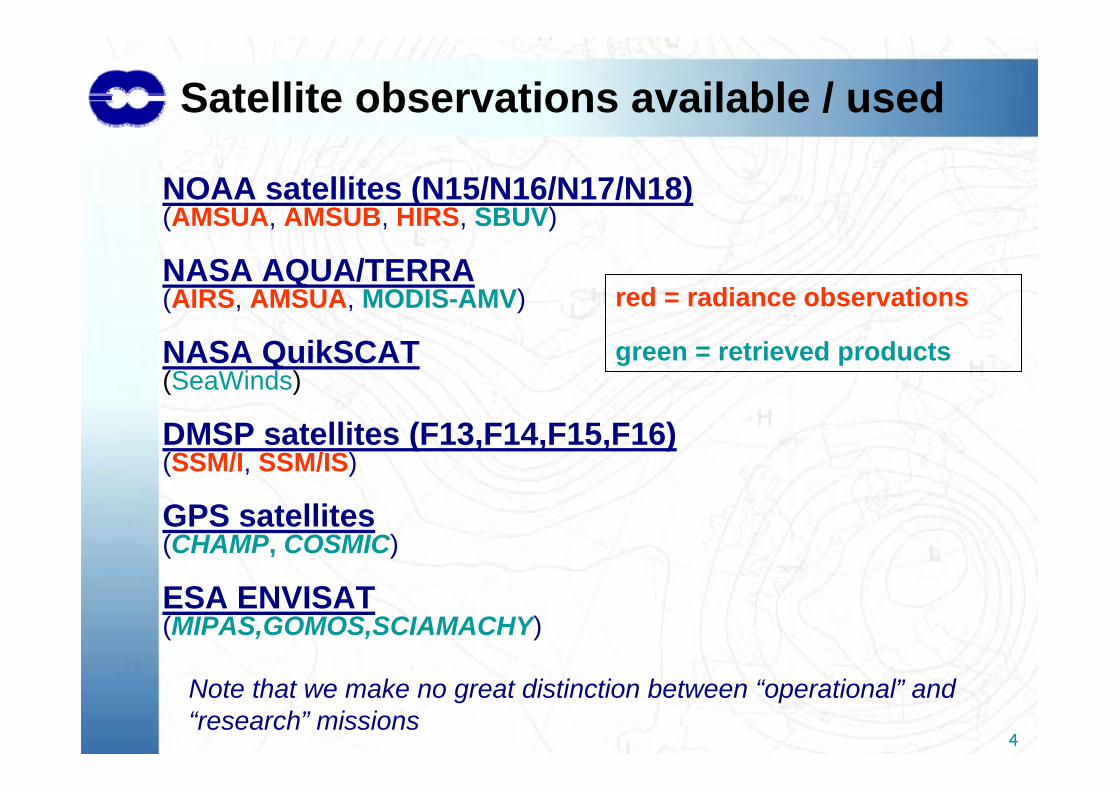
Satellite observations available / used
NOAA satellites (N15/N16/N17/N18)(AMSUA, AMSUB, HIRS, SBUV)
NASA AQUA/TERRA(AIRS, AMSUA, MODIS-AMV)
NASA QuikSCAT(SeaWinds)
DMSP satellites (F13,F14,F15,F16)(SSM/I, SSM/IS)
GPS satellites(CHAMP, COSMIC)
ESA ENVISAT(MIPAS,GOMOS,SCIAMACHY)
red = radiance observations
green = retrieved products
Note that we make no great distinction between “operational” and “research” missions
5
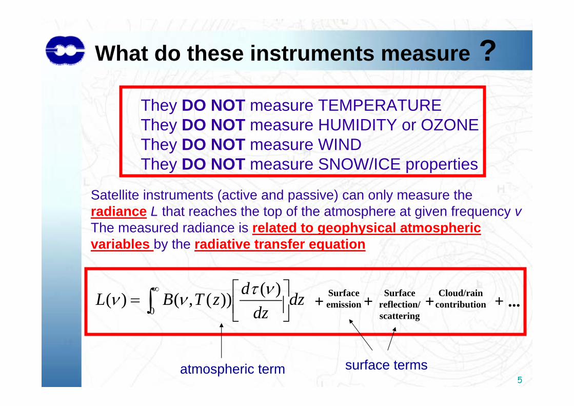
What do these instruments measure ?
dzdz
dzTBL ∫∞
⎥⎦⎤
⎢⎣⎡=
0
)())(,()( ντνν + Surfaceemission + Surface
reflection/scattering
+ Cloud/raincontribution
They DO NOT measure TEMPERATUREThey DO NOT measure HUMIDITY or OZONEThey DO NOT measure WINDThey DO NOT measure SNOW/ICE properties
Satellite instruments (active and passive) can only measure theradiance L that reaches the top of the atmosphere at given frequency vThe measured radiance is related to geophysical atmospheric variables by the radiative transfer equation
+ ...
atmospheric term surface terms
6
Radiance Observations
7
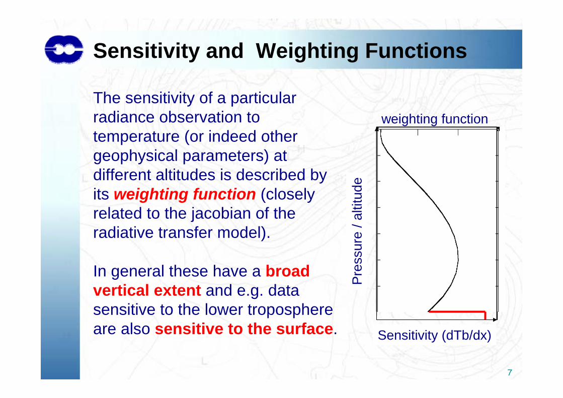
Sensitivity and Weighting Functions
The sensitivity of a particular radiance observation to temperature (or indeed other geophysical parameters) at different altitudes is described by its weighting function (closely related to the jacobian of the radiative transfer model).
In general these have a broad vertical extent and e.g. data sensitive to the lower troposphere are also sensitive to the surface. K(z)Sensitivity (dTb/dx)
Pre
ssur
e / a
ltitu
de
weighting function
8
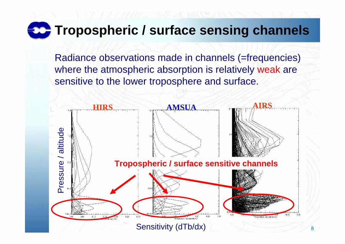
HIRS AMSUA AIRS
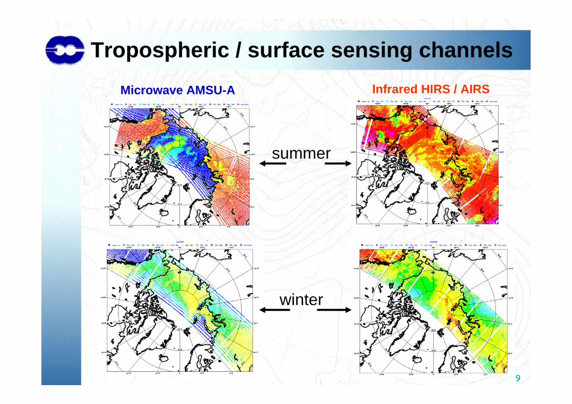
Radiance observations made in channels (=frequencies) where the atmospheric absorption is relatively weak are sensitive to the lower troposphere and surface.
Pre
ssur
e / a
ltitu
de
Sensitivity (dTb/dx)
Tropospheric / surface sensitive channels
Tropospheric / surface sensing channels
9
Tropospheric / surface sensing channelsMicrowave AMSU-A Infrared HIRS / AIRS
summer
winter
10
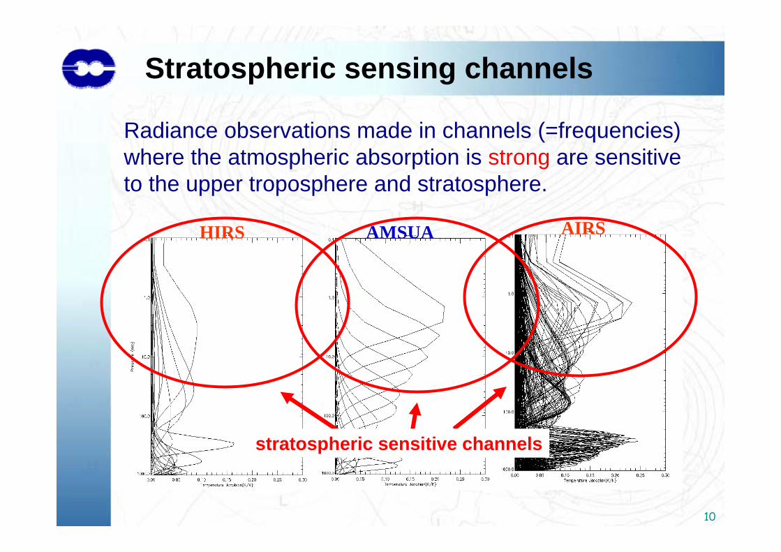
HIRS AMSUA AIRS
Radiance observations made in channels (=frequencies) where the atmospheric absorption is strong are sensitive to the upper troposphere and stratosphere.
Stratospheric sensing channels
stratospheric sensitive channels
11
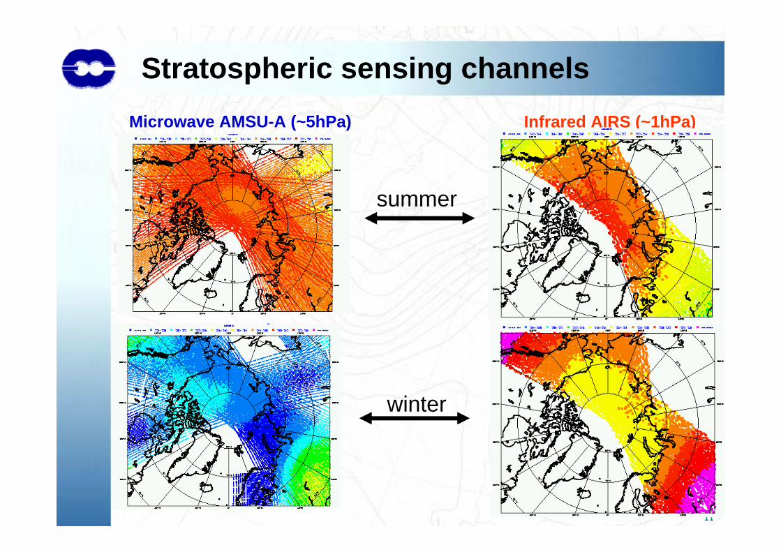
Microwave AMSU-A (~5hPa) Infrared AIRS (~1hPa)
summer
winter
Stratospheric sensing channels
12
Retrieved Products
13
Retrieved Products
Observed radiance observations are pre-converted to geophysical products (externally) before being provided to the NWP data assimilation system.
In most cases these have been phased out and replaced with the preferred direct assimilation of the original radiance observations.
However some have been retained and are still assimilated.
14
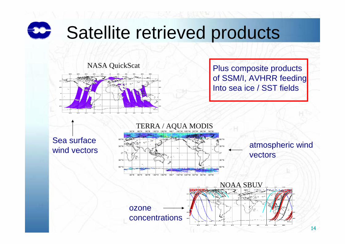
Satellite retrieved productsNASA QuickScat
TERRA / AQUA MODIS
NOAA SBUV
Plus composite products of SSM/I, AVHRR feedingInto sea ice / SST fields
atmospheric windvectors
ozone concentrations
Sea surface wind vectors
15
Satellite radiance assimilation
16
The data assimilation system
Jc
xyxyxxxxxJ
iiT
iii
bT
b
+
−−+
−−=−
−
∑ ])H[(])H[()()()(
1
1
RB
.
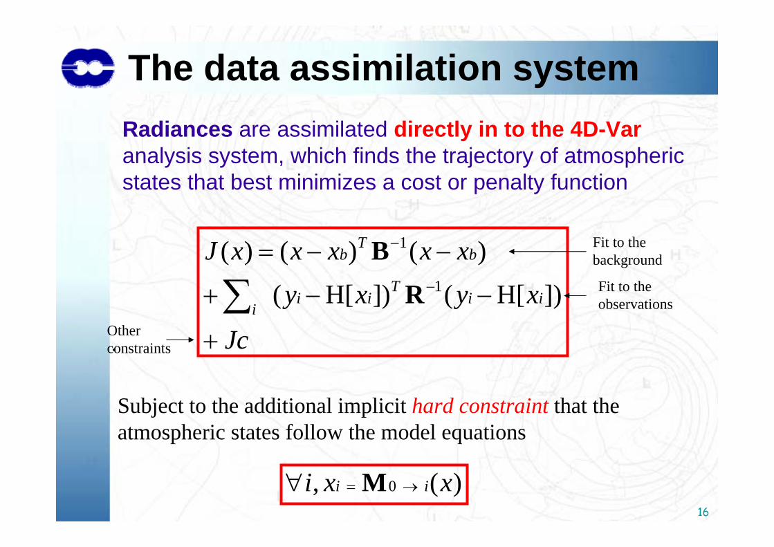
Subject to the additional implicit hard constraint that the atmospheric states follow the model equations
)(, 0 xxi ii →=∀ M
Radiances are assimilated directly in to the 4D-Varanalysis system, which finds the trajectory of atmospheric states that best minimizes a cost or penalty function
Fit to the background
Fit to the observations
Other constraints
17
The key elements of satellite radiance assimilation
•Radiative Transfer (or forward) Model
•Quality Control (data screening)
•Handling of surface ambiguity
•Observation errors (inc errors in RTM)
•Handling of systematic errors (biases)
•Background errors

18
Radiative Transfer
19
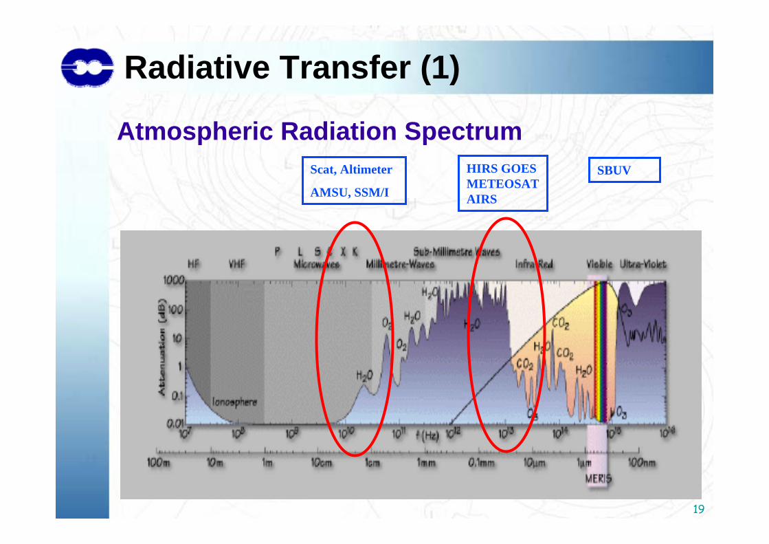
Scat, Altimeter
AMSU, SSM/I
HIRS GOES METEOSAT AIRS
SBUV
Atmospheric Radiation Spectrum
Radiative Transfer (1)
20
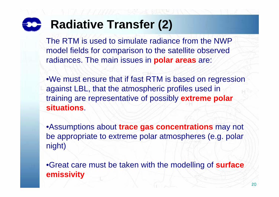
Radiative Transfer (2)The RTM is used to simulate radiance from the NWP model fields for comparison to the satellite observed radiances. The main issues in polar areas are:
•We must ensure that if fast RTM is based on regression against LBL, that the atmospheric profiles used in training are representative of possibly extreme polar situations.
•Assumptions about trace gas concentrations may not be appropriate to extreme polar atmospheres (e.g. polar night)
•Great care must be taken with the modelling of surface emissivity
21
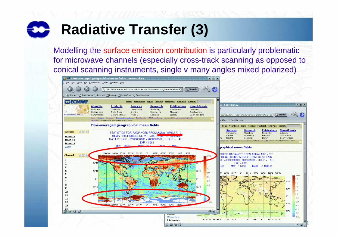
Modelling the surface emission contribution is particularly problematic for microwave channels (especially cross-track scanning as opposed to conical scanning instruments, single v many angles mixed polarized)
Radiative Transfer (3)
22
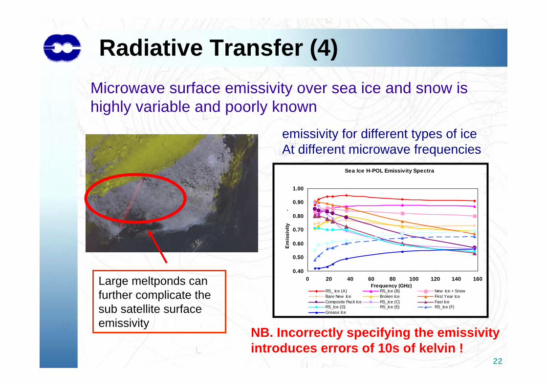
Microwave surface emissivity over sea ice and snow is highly variable and poorly known
Large meltponds can further complicate the sub satellite surface emissivity
Sea Ice H-POL Emissivity Spectra
0.40
0.50
0.60
0.70
0.80
0.90
1.00
0 20 40 60 80 100 120 140 160Frequency (GHz)
Em
issi
vity
-RS_ Ice (A) RS_Ice (B) New Ice + SnowBare New Ice Broken Ice First Year IceComposite Pack Ice RS_Ice (C) Fast IceRS_Ice (D) RS_Ice (E) RS_Ice (F)Grease Ice
Radiative Transfer (4)
emissivity for different types of ice At different microwave frequencies
NB. Incorrectly specifying the emissivityintroduces errors of 10s of kelvin !
23
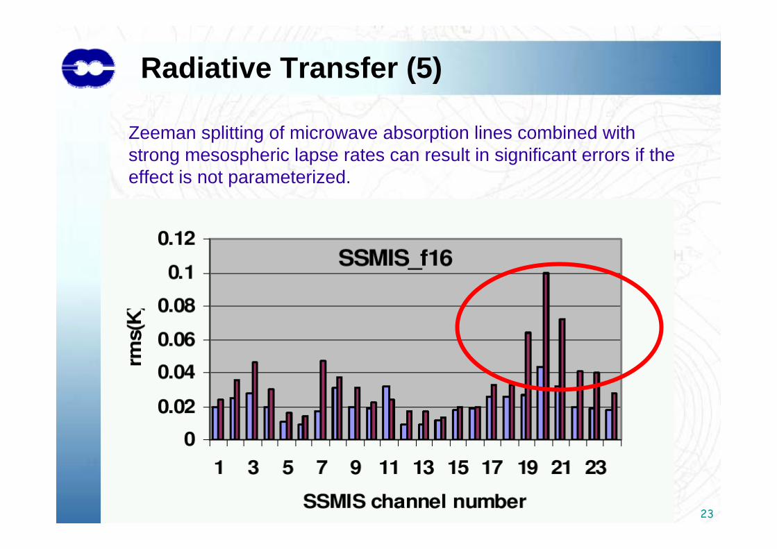
Zeeman splitting of microwave absorption lines combined with strong mesospheric lapse rates can result in significant errors if the effect is not parameterized.
Radiative Transfer (5)

24
Quality Control
25
Quality Control (1)With modern day instruments QC is more concerned with identifying situations where our assumptions (both discrete and statistical) are invalid, rather than identifying badobservations….e.g. …
•Cloud contamination (IR and MW)
•Rain (precipitation) contamination (MW)
•Poor surface characterization (or heterogeneous scenes)
26
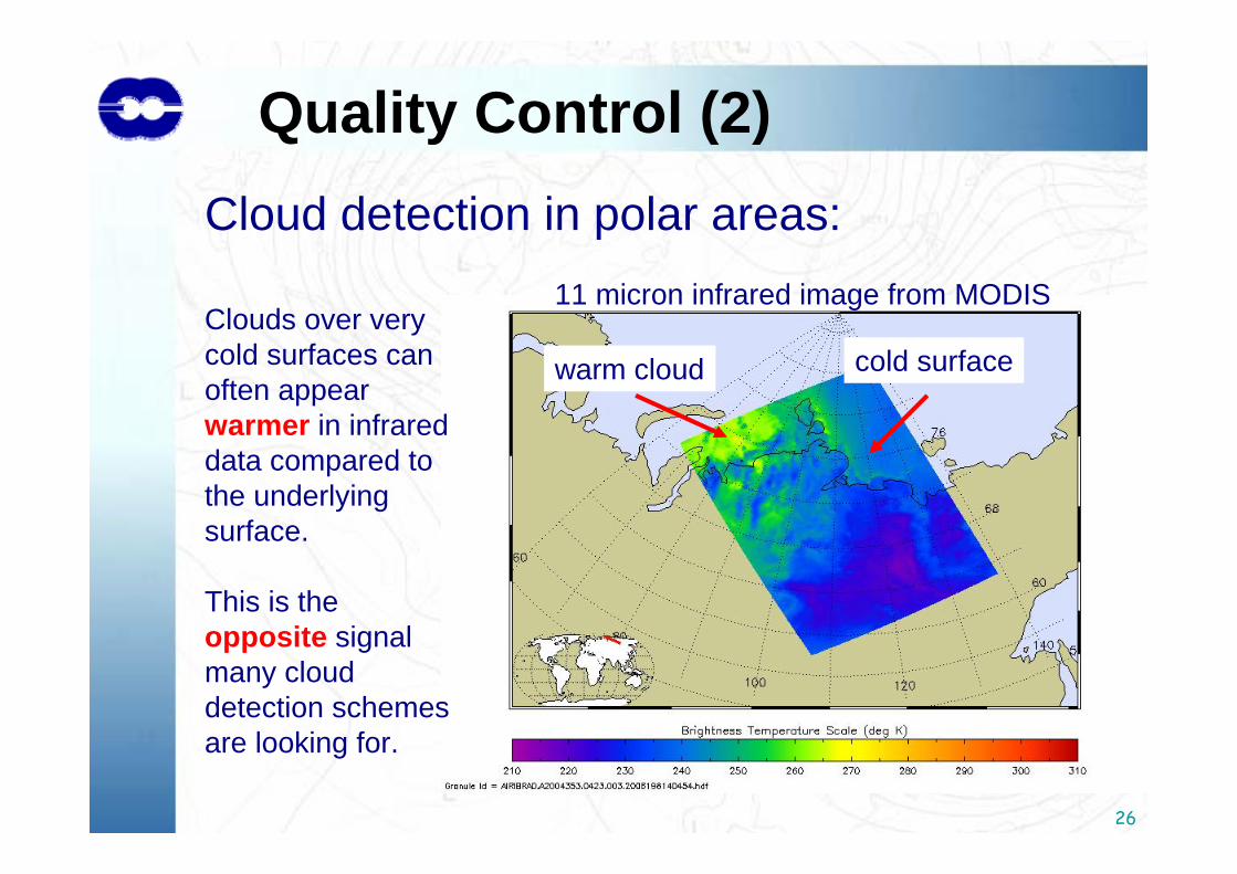
Quality Control (2)Cloud detection in polar areas:
11 micron infrared image from MODISClouds over very cold surfaces can often appear warmer in infrared data compared to the underlying surface.
This is the opposite signal many cloud detection schemes are looking for.
warm cloud cold surface
27
Cloud detection algorithms generally rely on an accurate a priori knowledge of the underlying surface emission.
Errors in the modelling the underlying surface emission (T* or E) can compromise our ability to safely detect clouds
Single channel cloud detection (i.e. window channel checks) can be dangerous (cloud compensates in window channel, but not channels above)
If these problems are severe, we may have to blacklist (i.e. a priori reject) the radiance observations
Quality Control (3)
28
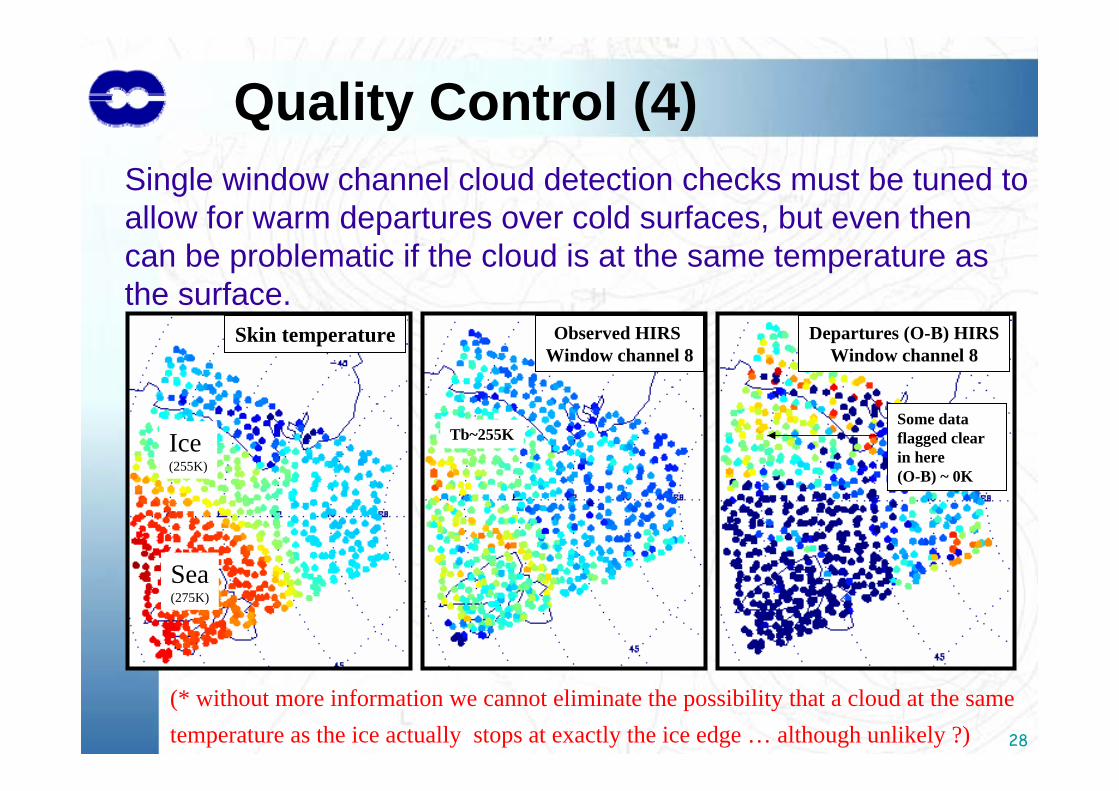
Skin temperature Observed HIRS Window channel 8
Departures (O-B) HIRSWindow channel 8
Ice(255K)
Sea(275K)
(* without more information we cannot eliminate the possibility that a cloud at the same temperature as the ice actually stops at exactly the ice edge … although unlikely ?)
Some data flagged clear in here (O-B) ~ 0K
Tb~255K
Single window channel cloud detection checks must be tuned to allow for warm departures over cold surfaces, but even then can be problematic if the cloud is at the same temperature as the surface.
Quality Control (4)
29
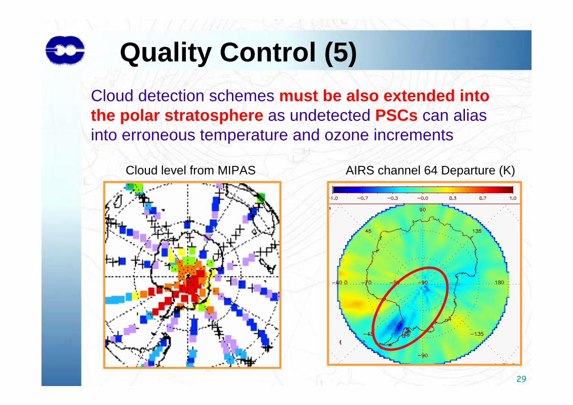
AIRS channel 64 Departure (K)Cloud level from MIPAS
Cloud detection schemes must be also extended into the polar stratosphere as undetected PSCs can alias into erroneous temperature and ozone increments
Quality Control (5)
30
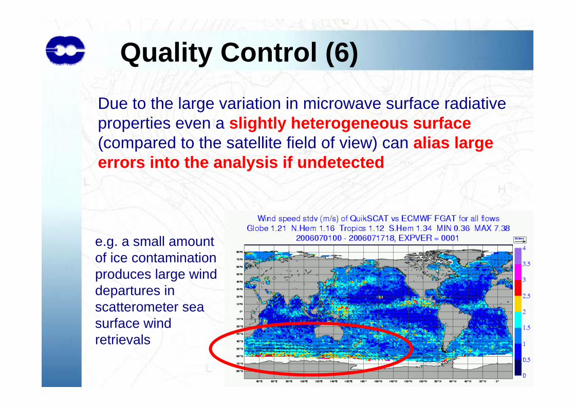
Quality Control (6)Due to the large variation in microwave surface radiativeproperties even a slightly heterogeneous surface(compared to the satellite field of view) can alias large errors into the analysis if undetected
e.g. a small amount of ice contamination produces large wind departures in scatterometer sea surface wind retrievals
31
Handling Surface Ambiguity (1)
The variability of the polar surface (particularly in terms of microwave surface emissivity) is significant. Channels designed to provide temperature information in the mid-troposphere still have ~ 10% sensitivity to the surface.
In channels such as AMSU-5 and MSU-2 (very important for NWP and reanalysis) the surface variability (e.g. going from sea to ice) is ~ 2K whereas the atmospheric variability (i.e. due to temperature variations) is typically less than 0.5K.
Thus errors in modelling the surface emission in these channels can completely dominate the useful atmospheric signal!
32
Handling Surface Ambiguity (2)
Options for handling the surface contribution:
1. Model the surface emissivity explicitly from our knowledge of the surface conditions (e.g. ice type, snow cover …) and then use a fixed value in the RTM
2. Use indicators from the radiance observations to estimate or classify the surface and then fix in the RTM
3. Add emissivity to the analysis variables and estimate it simultaneously with other geophysical variables within the assimilation
4. Use radiances from sensors better suited to handling surface effects (e.g. conical scanning SSM/IS rather than cross-track scanning AMSUA)
33
Systematic Errors(biases)
34
Systematic Errors (1)
Biases in satellite observations and / or RTM are a serious problem as they can quickly propagate into large scale biases in the analysis.
Traditionally satellite bias corrections are estimated from monitoring data against the NWP system (in the absence of any other globally available ground truth)
35
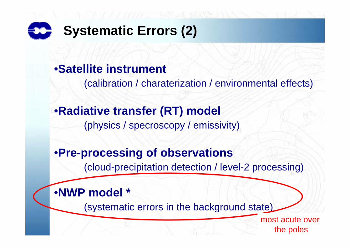
•Satellite instrument(calibration / charaterization / environmental effects)
•Radiative transfer (RT) model(physics / specroscopy / emissivity)
•Pre-processing of observations(cloud-precipitation detection / level-2 processing)
•NWP model *(systematic errors in the background state)
most acute over the poles
Systematic Errors (2)
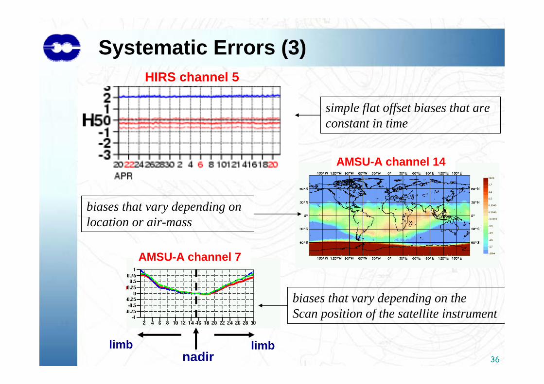
36nadirlimblimb
AMSU-A channel 14
biases that vary depending on the Scan position of the satellite instrument
biases that vary depending on location or air-mass
simple flat offset biases that are constant in time
AMSU-A channel 7
HIRS channel 5
Systematic Errors (3)
37
Systematic Errors (4)
Over the polar regions (particularly in the stratosphere) we can have large systematic errors in the NWP model (suggesting apparentair-mass and scan dependent biases in the satellite observations)
It is important that we do not derive observation bias corrections that actually compensate for systematic errors in the NWP model as this will perpetuate or even reinforce the system bias
38
60°S60°S
30°S 30°S
0°0°
30°N 30°N
60°N60°N
150°W
150°W 120°W
120°W 90°W
90°W 60°W
60°W 30°W
30°W 0°
0° 30°E
30°E 60°E
60°E 90°E
90°E 120°E
120°E 150°E
150°E
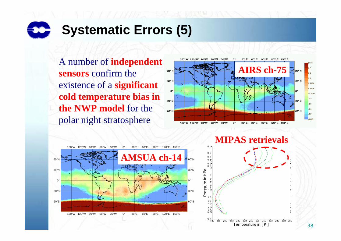
AMSUA ch-14
AIRS ch-75
MIPAS retrievals
A number of independent sensors confirm the existence of a significant cold temperature bias in the NWP model for the polar night stratosphere
Systematic Errors (5)
39
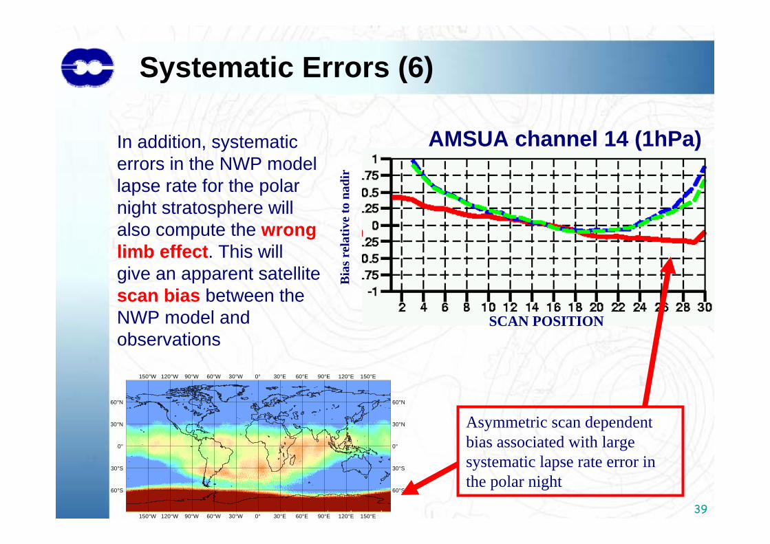
In addition, systematic errors in the NWP model lapse rate for the polar night stratosphere will also compute the wrong limb effect. This will give an apparent satellite scan bias between the NWP model and observations
60°S60°S
30°S 30°S
0°0°
30°N 30°N
60°N60°N
150°W
150°W 120°W
120°W 90°W
90°W 60°W
60°W 30°W
30°W 0°
0° 30°E
30°E 60°E
60°E 90°E
90°E 120°E
120°E 150°E
150°E
SCAN POSITIONB
ias r
elat
ive
to n
adir
AMSUA channel 14 (1hPa)
Asymmetric scan dependent bias associated with large systematic lapse rate error in the polar night
Systematic Errors (6)
40
Force the (uncorrected) satellite observations into the data assimilation system to correct the NWP model bias (can be problematic).
or
Pragmatically apply a bias correction to the observations to compensate for the model error (produces a biased analysis).
Systematic Errors (7)
So what can we do if the NWP model has a significant bias ?
41
60°S60°S
30°S 30°S
0°0°
30°N 30°N
60°N60°N
150°W
150°W 120°W
120°W 90°W
90°W 60°W
60°W 30°W
30°W 0°
0° 30°E
30°E 60°E
60°E 90°E
90°E 120°E
120°E 150°E
150°E
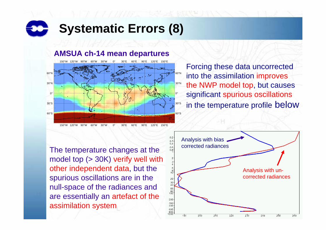
AMSUA ch-14 mean departuresForcing these data uncorrected into the assimilation improves the NWP model top, but causes significant spurious oscillationsin the temperature profile below
Systematic Errors (8)
Analysis with bias corrected radiances
Analysis with un-corrected radiances
The temperature changes at the model top (> 30K) verify well with other independent data, but the spurious oscillations are in the null-space of the radiances and are essentially an artefact of the assimilation system
42
Miscellaneous issues in polar areas
•Observation weights (errors and spatial correlations) and thinning to account for high density of radiance observations over the poles
•Constituent estimation (humidity, CO2 and ozone) from passive sensors is very difficult in some isothermal polar atmospheres.
•Assimilation of rain / snow affected microwave radiances very difficult over bright frozen surfaces
•A general lack of verification / validation information
43
… but on the brighter side …
44
Examples of the successful exploitation of satellite data in
polar regions
45
Polar successes with satellite data
Validation of ERA-40 and operational analyses suggest that satellite radiance observations are used well in polar areas andare a vital component of the observing system
Surface mapping products now taken for granted and are a main-stay of polar studies
Monitoring / forecasting sudden warming of the polar stratosphere
Polar ozone analysis
MODIS winds products have a good impact on forecasts
Constraining the polar wind field with temperature sounder data
Synergy between nadir and limb sounding data
Tuning physical parameterizations with satellite observations
46
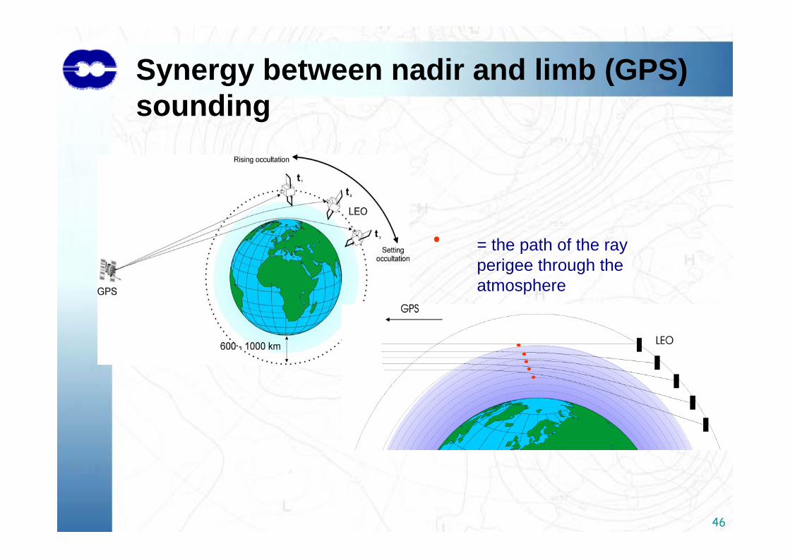
= the path of the ray perigee through the atmosphere
Synergy between nadir and limb (GPS) sounding
47
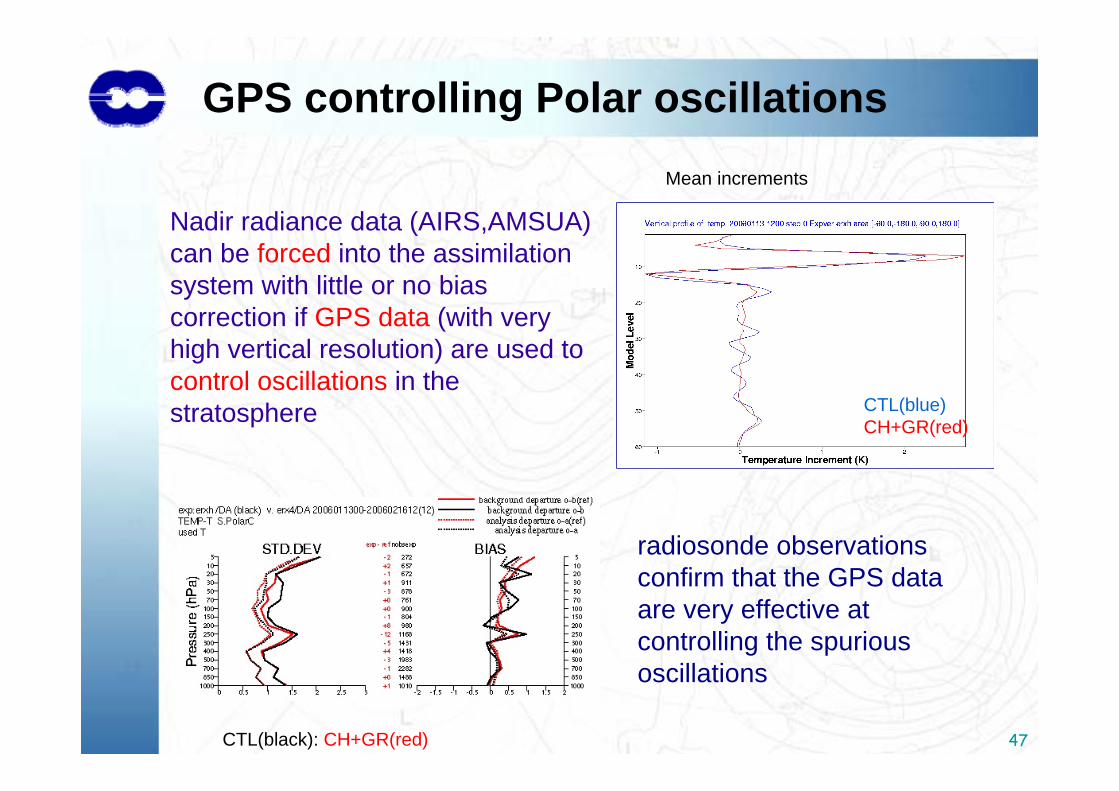
GPS controlling Polar oscillationsMean increments
CTL(blue)CH+GR(red)
CTL(black): CH+GR(red)
Nadir radiance data (AIRS,AMSUA) can be forced into the assimilation system with little or no bias correction if GPS data (with very high vertical resolution) are used to control oscillations in the stratosphere
radiosonde observations confirm that the GPS data are very effective at controlling the spurious oscillations
48
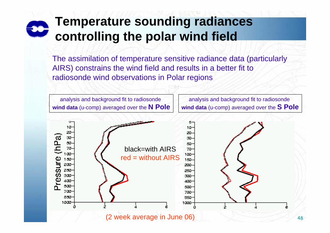
Temperature sounding radiances controlling the polar wind field
analysis and background fit to radiosondewind data (u-comp) averaged over the N Pole
analysis and background fit to radiosondewind data (u-comp) averaged over the S Pole
black=with AIRSred = without AIRS
(2 week average in June 06)
The assimilation of temperature sensitive radiance data (particularly AIRS) constrains the wind field and results in a better fit to radiosonde wind observations in Polar regions
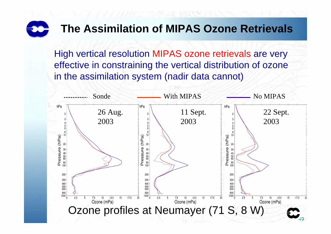
49Ozone profiles at Neumayer (71 S, 8 W)
26 Aug. 2003
11 Sept. 2003
22 Sept. 2003
Sonde With MIPAS No MIPAS
The Assimilation of MIPAS Ozone Retrievals
High vertical resolution MIPAS ozone retrievals are very effective in constraining the vertical distribution of ozone in the assimilation system (nadir data cannot)
50
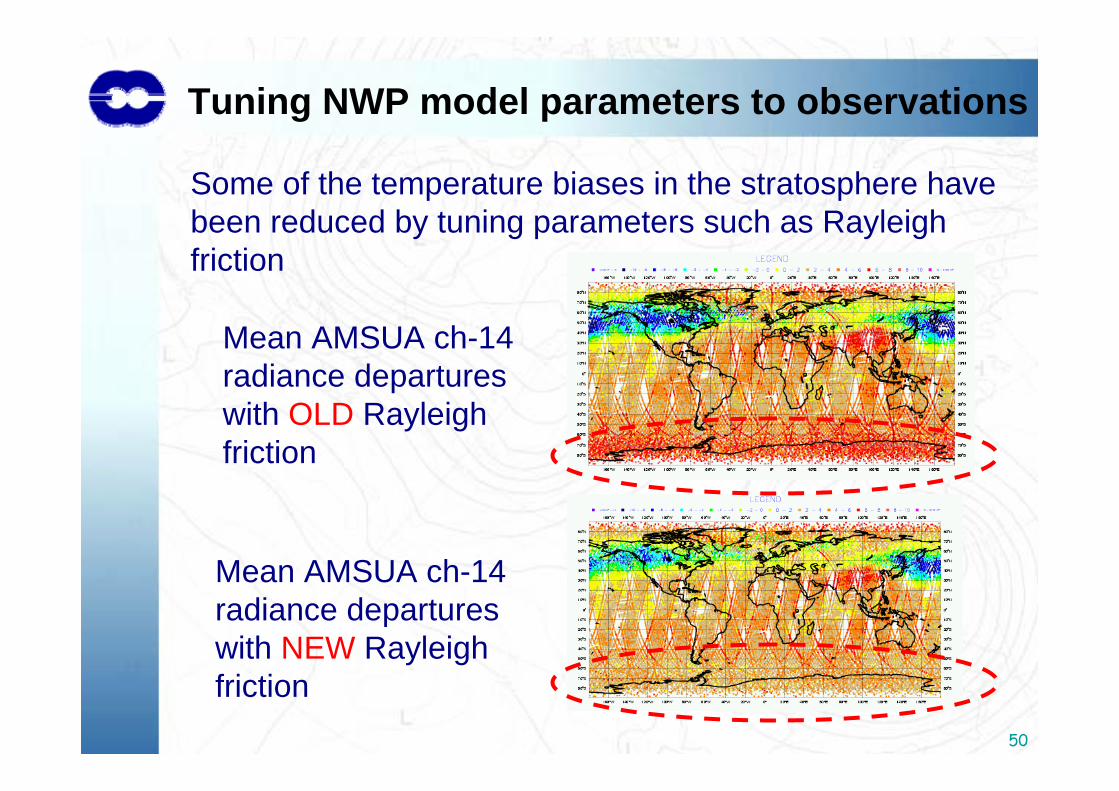
Tuning NWP model parameters to observations
Mean AMSUA ch-14 radiance departures with OLD Rayleighfriction
Some of the temperature biases in the stratosphere have been reduced by tuning parameters such as Rayleighfriction
Mean AMSUA ch-14 radiance departures with NEW Rayleighfriction
51
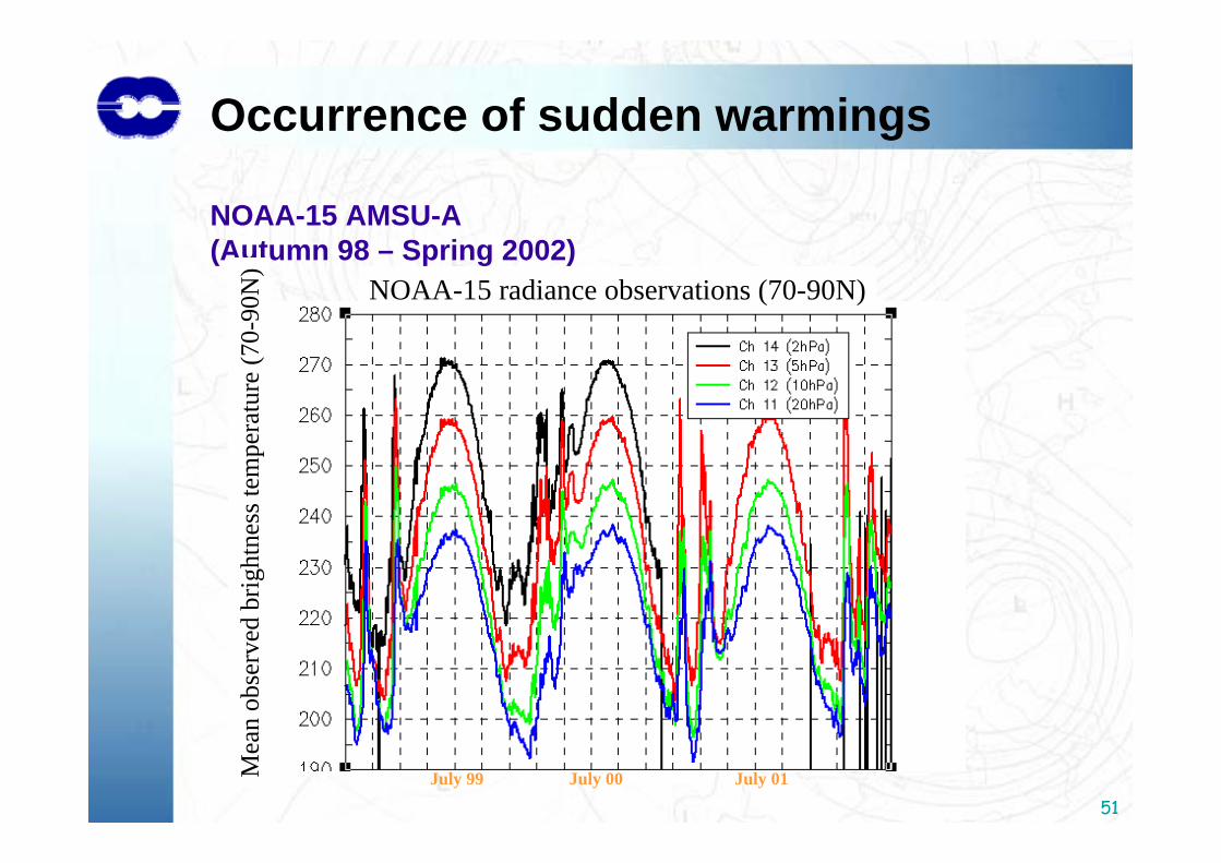
Occurrence of sudden warmings
NOAA-15 AMSU-A (Autumn 98 – Spring 2002)
July 99 July 00 July 01Mea
n ob
serv
ed b
right
ness
tem
pera
ture
(70-
90N
)NOAA-15 radiance observations (70-90N)
52
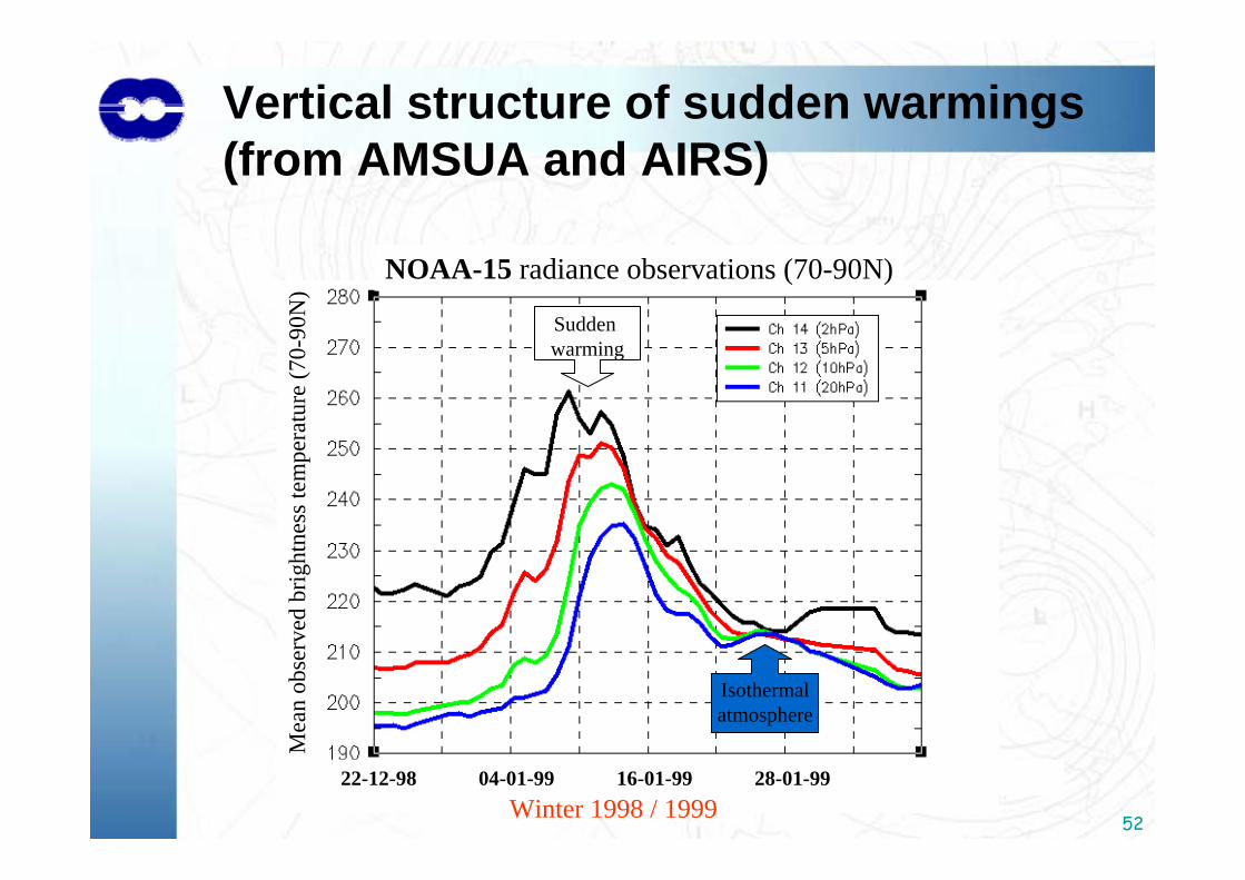
Vertical structure of sudden warmings(from AMSUA and AIRS)
Isothermalatmosphere
NOAA-15 radiance observations (70-90N)M
ean
obse
rved
brig
htne
ss te
mpe
ratu
re (7
0-90
N)
22-12-98 04-01-99 16-01-99 28-01-99 Winter 1998 / 1999
Sudden warming
53
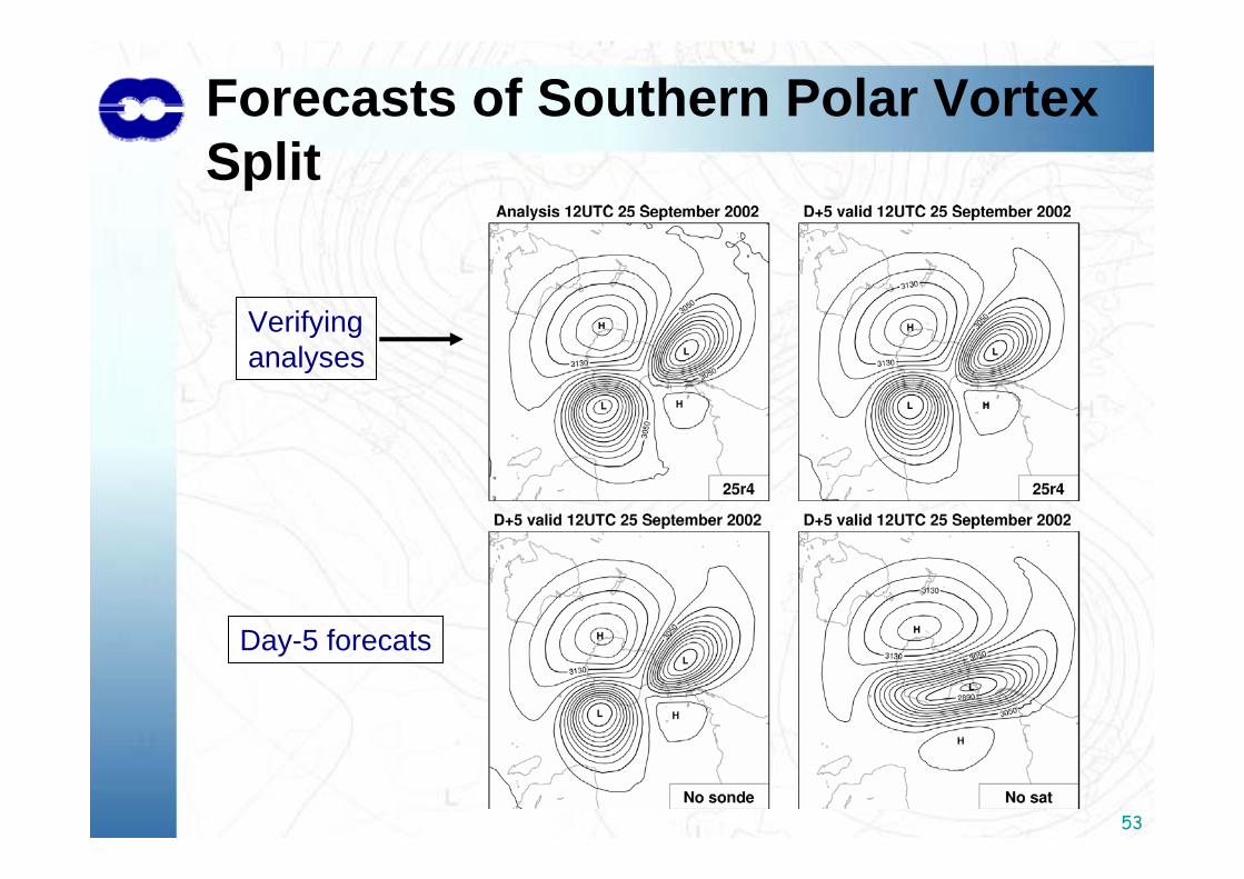
Forecasts of Southern Polar Vortex Split
Verifyinganalyses
Day-5 forecats
54
Summary
•There is a vast amount of satellite data available at the poles,however the polar regions present some particular assimilation challenges:
•The variability of the polar surface (and our poor knowledge of it) makes mid-lower tropospheric radiance data difficult to use safely (both from a RT perspective and the detection of clouds when thesurface variability far exceeds the atmospheric signal).
•However, microwave and infrared radiance data sensitive to the upper troposphere and stratosphere are used extensively and havea significant measurable impact on Polar NWP / reanalysis.
•Systematic errors in the NWP model can be large in the polar stratosphere and care must be taken how the radiance data are bias corrected and introduced into the assimilation system.
55
End
56
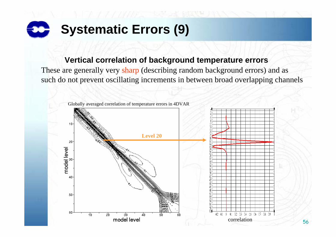
Vertical correlation of background temperature errorsThese are generally very sharp (describing random background errors) and as such do not prevent oscillating increments in between broad overlapping channels
Level 20
correlation
Globally averaged correlation of temperature errors in 4DVAR
Systematic Errors (9)
57
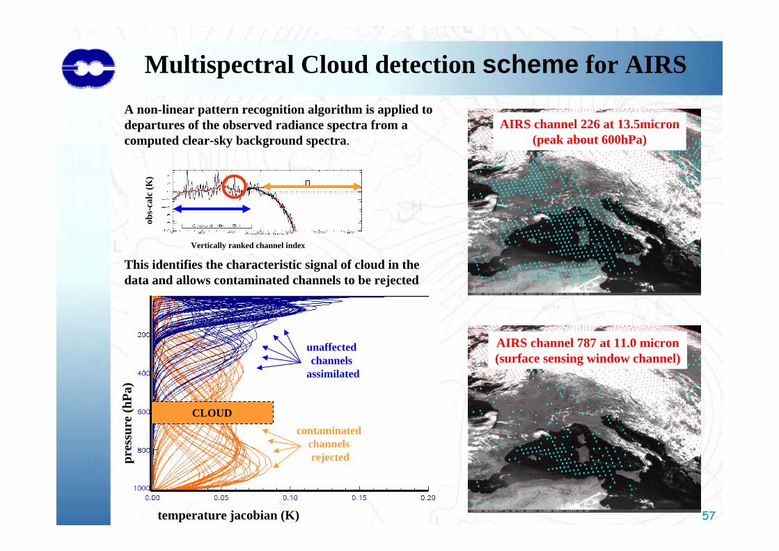
CLOUD
AIRS channel 226 at 13.5micron(peak about 600hPa)
AIRS channel 787 at 11.0 micron(surface sensing window channel)
temperature jacobian (K)
pres
sure
(hPa
)
unaffected channels
assimilated
contaminated channels rejected
Multispectral Cloud detection scheme for AIRSA non-linear pattern recognition algorithm is applied to departures of the observed radiance spectra from a computed clear-sky background spectra.
This identifies the characteristic signal of cloud in the data and allows contaminated channels to be rejected
obs-
calc
(K)
Vertically ranked channel index
58
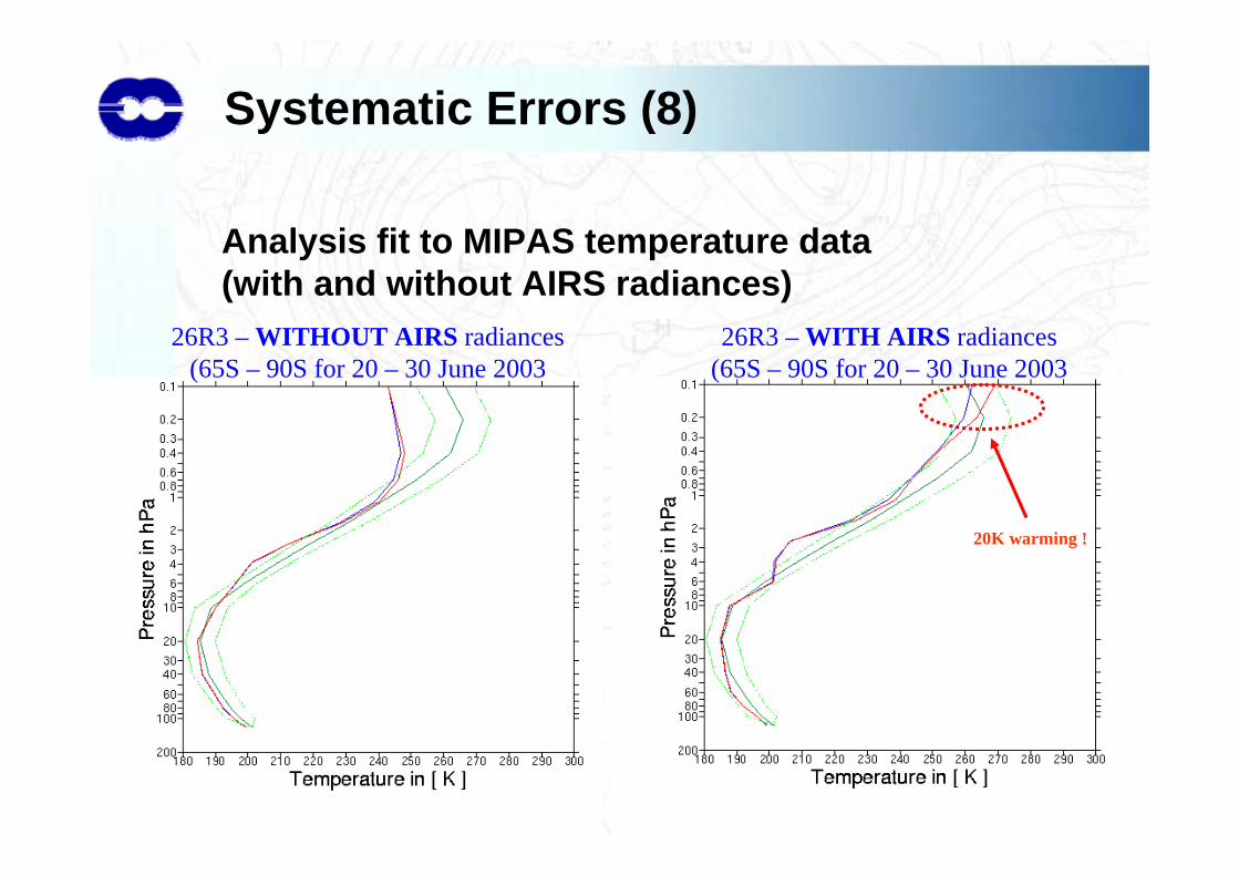
Analysis fit to MIPAS temperature data(with and without AIRS radiances)
26R3 – WITHOUT AIRS radiances(65S – 90S for 20 – 30 June 2003
26R3 – WITH AIRS radiances(65S – 90S for 20 – 30 June 2003
20K warming !
Systematic Errors (8)
59
Recommended