Neuron
Article
Variance as a Signature of Neural Computationsduring Decision MakingAnne. K. Churchland,1,6,* R. Kiani,2,5 R. Chaudhuri,3 Xiao-Jing Wang,3 Alexandre Pouget,4 and M.N. Shadlen1,51Department of Physiology and Biophysics, University of Washington Medical School, National Primate Research Center, Seattle,
WA 98195-7290, USA2Department of Neurobiology, Stanford University, Fairchild Building, Room D200, Stanford, CA 94305, USA3Department of Neurobiology, Yale University, New Haven, CT 06520-8001, USA4Department of Brain and Cognitive Sciences, University of Rochester, Rochester, NY 14627, USA5Howard Hughes Medical Institute6Present address: Cold Spring Harbor Laboratory, Cold Spring Harbor, NY 11724, USA*Correspondence: [email protected]
DOI 10.1016/j.neuron.2010.12.037
SUMMARY
Traditionally, insights into neural computation havebeen furnished by averaged firing rates frommany stimulus repetitions or trials. We pursue ananalysis of neural response variance to unveil neuralcomputations that cannot be discerned frommeasures of average firing rate. We analyzedsingle-neuron recordings from the lateral intraparie-tal area (LIP), during a perceptual decision-makingtask. Spike count variance was divided into twocomponents using the law of total variance fordoubly stochastic processes: (1) variance of countsthat would be produced by a stochastic pointprocesswith a given rate, and loosely (2) the varianceof the rates that would produce those counts (i.e.,‘‘conditional expectation’’). The variance and corre-lation of the conditional expectation exposed severalneural mechanisms: mixtures of firing rate statespreceding the decision, accumulation of stochastic‘‘evidence’’ during decision formation, and a stereo-typed response at decision end. These analyses helpto differentiate among several alternative decision-making models.
INTRODUCTION
The quantitative study of cortical neural systems rests largely on
establishing systematic relationships between changes in neural
firing rate and changes in a stimulus attribute, motor response, or
decision. For example, responses of neurons in primary somato-
sensory cortex lay the foundation for understanding vibrotactile
sensation because mean firing rates are significantly higher for
more intense tactile stimuli (Romo and Salinas, 2001). Likewise,
responses in the middle temporal area (MT) are thought to
underlie some aspects of motion perception, in part because
their mean firing rates vary with motion strength in a manner
that explains choice accuracy in a direction discrimination task
818 Neuron 69, 818–831, February 24, 2011 ª2011 Elsevier Inc.
(Britten et al., 1992). It follows that the variability of firing rate
across repetitions might bear on the fidelity of these neural
signals (Barlow, 1956; Bulmer et al., 1957; Tolhurst et al.,
1983). Together, the mean and variance of neural responses
furnish rich insight into the limits of perception, motor control
and decision making (Faisal et al., 2008; Glimcher, 2005; Parker
and Newsome, 1998; Shadlen and Newsome, 1998).
Response variability can also furnish insight into the neural
computations themselves. For example, the irregular discharge
of neurons bears on theories of coding, synaptic integration
and circuit function (Shadlen and Newsome, 1998; Softky
and Koch, 1993). Recently, it has been suggested that the
time course of the variance during a complex computation
can expose properties of the signal transformation, such as a
sign of a fixed point or attractor (Churchland et al., 2010). Here,
we exploit a principled measure of response variability that
identifies a component of variance that distinguishes various
classes of neural computations. We apply this measure to
study the responses of neurons in the lateral intraparietal area
(LIP) of the macaque during a perceptual decision-making task
(Figure 1).
Because the momentary evidence in the random-dot motion
stimulus we use is noisy and temporally uncorrelated, a reason-
able strategy for making decisions is to accumulate evidence
over time. The time-dependent pattern of mean firing rates is
consistent with a bounded integration mechanism (Figure 1)
(Gold and Shadlen, 2007; Smith and Ratcliff, 2004). After an initial
dip, firing rates change gradually during decision formation at
a rate that depends on stimulus strength (Figure 1, middle
column). On trials when the monkey decides in favor of the
choice target in the neuron’s RF (a Tin choice), mean firing rates
reach a high value at the end of the decision (Figure 1, right
column) that is similar for all motion strengths and reaction times
(RTs).
While bounded integration offers a parsimonious explanation
of the choice and decision time, the mean response could be
explained by a variety of alternative mechanisms that do not
involve integration of noisy evidence. For example, the rise of
mean firing rates to a threshold value could imply preparation
for a saccadic eye movement (Hanes and Schall, 1996). Or,
the rise might represent a change in the gain of a sensory
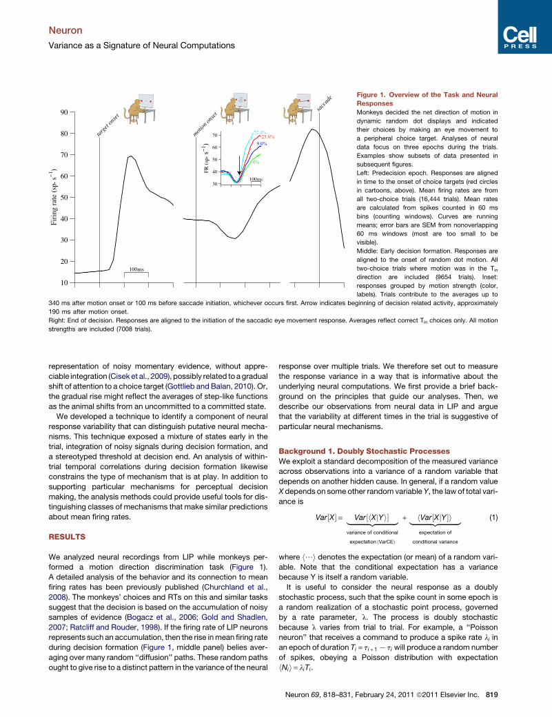
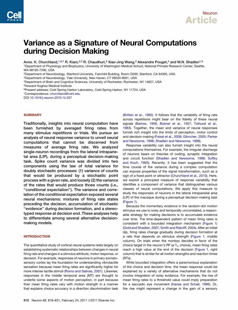
Figure 1. Overview of the Task and Neural
Responses
Monkeys decided the net direction of motion in
dynamic random dot displays and indicated
their choices by making an eye movement to
a peripheral choice target. Analyses of neural
data focus on three epochs during the trials.
Examples show subsets of data presented in
subsequent figures.
Left: Predecision epoch. Responses are aligned
in time to the onset of choice targets (red circles
in cartoons, above). Mean firing rates are from
all two-choice trials (16,444 trials). Mean rates
are calculated from spikes counted in 60 ms
bins (counting windows). Curves are running
means; error bars are SEM from nonoverlapping
60 ms windows (most are too small to be
visible).
Middle: Early decision formation. Responses are
aligned to the onset of random dot motion. All
two-choice trials where motion was in the Tindirection are included (9654 trials). Inset:
responses grouped by motion strength (color,
labels). Trials contribute to the averages up to
340 ms after motion onset or 100 ms before saccade initiation, whichever occurs first. Arrow indicates beginning of decision related activity, approximately
190 ms after motion onset.
Right: End of decision. Responses are aligned to the initiation of the saccadic eye movement response. Averages reflect correct Tin choices only. All motion
strengths are included (7008 trials).
Neuron
Variance as a Signature of Neural Computations
representation of noisy momentary evidence, without appre-
ciable integration (Cisek et al., 2009), possibly related to agradual
shift of attention to a choice target (Gottlieb and Balan, 2010). Or,
the gradual rise might reflect the averages of step-like functions
as the animal shifts from an uncommitted to a committed state.
We developed a technique to identify a component of neural
response variability that can distinguish putative neural mecha-
nisms. This technique exposed a mixture of states early in the
trial, integration of noisy signals during decision formation, and
a stereotyped threshold at decision end. An analysis of within-
trial temporal correlations during decision formation likewise
constrains the type of mechanism that is at play. In addition to
supporting particular mechanisms for perceptual decision
making, the analysis methods could provide useful tools for dis-
tinguishing classes of mechanisms that make similar predictions
about mean firing rates.
RESULTS
We analyzed neural recordings from LIP while monkeys per-
formed a motion direction discrimination task (Figure 1).
A detailed analysis of the behavior and its connection to mean
firing rates has been previously published (Churchland et al.,
2008). The monkeys’ choices and RTs on this and similar tasks
suggest that the decision is based on the accumulation of noisy
samples of evidence (Bogacz et al., 2006; Gold and Shadlen,
2007; Ratcliff and Rouder, 1998). If the firing rate of LIP neurons
represents such an accumulation, then the rise inmean firing rate
during decision formation (Figure 1, middle panel) belies aver-
aging over many random ‘‘diffusion’’ paths. These random paths
ought to give rise to a distinct pattern in the variance of the neural
response over multiple trials. We therefore set out to measure
the response variance in a way that is informative about the
underlying neural computations. We first provide a brief back-
ground on the principles that guide our analyses. Then, we
describe our observations from neural data in LIP and argue
that the variability at different times in the trial is suggestive of
particular neural mechanisms.
Background 1. Doubly Stochastic ProcessesWe exploit a standard decomposition of the measured variance
across observations into a variance of a random variable that
depends on another hidden cause. In general, if a random value
X depends on some other random variable Y, the law of total vari-
ance is
Var½X�= Var½hXjYi�|fflfflfflfflfflfflfflfflfflfflfflffl{zfflfflfflfflfflfflfflfflfflfflfflffl}variance of conditional
expectation ðVarCEÞ
+ hVar½XjY �i|fflfflfflfflfflfflfflfflfflfflfflffl{zfflfflfflfflfflfflfflfflfflfflfflffl}expectation of
conditional variance
(1)
where h/i denotes the expectation (or mean) of a random vari-
able. Note that the conditional expectation has a variance
because Y is itself a random variable.
It is useful to consider the neural response as a doubly
stochastic process, such that the spike count in some epoch is
a random realization of a stochastic point process, governed
by a rate parameter, l. The process is doubly stochastic
because l varies from trial to trial. For example, a ‘‘Poisson
neuron’’ that receives a command to produce a spike rate li in
an epoch of duration Ti = ti + 1 � ti will produce a random number
of spikes, obeying a Poisson distribution with expectation
hNii= liTi.
Neuron 69, 818–831, February 24, 2011 ª2011 Elsevier Inc. 819
A F
B
C
D
E
Figure 2. Examples of Doubly Stochastic
Point Processes
(A–E) Each process is characterized by a rate func-
tion that may vary from trial to trial and a random
point process that realizes that rate. Both sources
of variability contribute to total spike count vari-
ance. For each process, theoretical rate functions
are shown with simulations of a nonstationary
Poisson point process. Mean spike rate and spike
count variance are calculated in nonoverlapping
windows using the same method as for analysis
of data in subsequent figures (60 ms; 20,000 simu-
lated trials). Ten random spike trains are shown in
the rasters below the panels.
(A) Constant rate without trial-to-trial variation.
Spike count variability arises only from the
stochastic point process (PPV), hence VarCE = 0.
(B) Constant rate with trial-to-trial variation. A
random value perturbs each rate function for the
duration of the trial. Gray traces: examples of
rate functions used to generate spikes. Total vari-
ance comprises PPV and VarCE.
(C) Same as (B) but with time varying rates.
(D) Same as (C) except that a new random pertur-
bation is sampled every 10 ms.
(E) Drift diffusion. Rate is the sum of a deterministic
‘‘drift’’ function (same linear rise as in B and C)
plus the cumulative sum of independent,
random values drawn from a Normal distribution
(mean = 0). Individual rate traces resemble one-
dimensional Brownian motion (with drift).
(F) VarCE for the five examples. The VarCE
captures the portion of total variance owing to
variation in the rate functions across trials. Thick
dashed lines show theoretical values (s2hNi) of
VarCE for doubly stochastic Poisson point
processes. Thin solid lines show VarCE estimated
by application of Equation 5 to the simulated spike
trains (s2hNi) assuming f= 1. Note that in real data, f
is not known. Counting window = 60ms. Line color
corresponds to the colors used in (A)–(E).
Neuron
Variance as a Signature of Neural Computations
Corresponding to Equation 1, the variance of that spike count
can be described as
s2Ni|{z}
Total measured
variance
= s2hNii|ffl{zffl}
VarCE
+Ds2Ni jli
E|fflfflfflffl{zfflfflfflffl}
Point process
variance ðPPVÞ
(2)
where Ni is the number of spikes in the epoch and li is the firing
rate. Note that means and variances are over trials, using the
same time epoch. We refer to the first term on the right side of
Equation 2 as the ‘‘variance of the conditional expectation’’
(VarCE) because it represents the variance of a theoretical quan-
tity that the neuron realizes through its spike discharge. We write
s2hNii as shorthand for s2hNi jlii because the expectation of any
count sample, given rate li on that trial, is hNijlii= liTi. The last
term in Equation 2 is the expectation of the conditional variance,
but we shall refer to it as the ‘‘point process variance’’ (PPV) to
convey the intuition: even if li does not vary from trial to trial,
the Ni would still vary from trial to trial according to some
distribution.
820 Neuron 69, 818–831, February 24, 2011 ª2011 Elsevier Inc.
For a Poisson neuron the PPV conforms to the Poisson distri-
bution: the PPV equals the expectation of the counts (Daley and
Vere-Jones, 2003). If the expectation is the same on every trial,
then hs2Ni jli i= liTi = hNii and the VarCE is zero. This case is illus-
trated in Figure 2A and the blue dashed trace in Figure 2F. Each
point process (rasters) is produced by realization of the same
rate. There is variability from trial to trial, but it is attributed solely
to the PPV.
Next, consider an example in which the rate is different on
each trial (Figure 2B). For simplicity, suppose that the rate is
stationary throughout the duration of each trial, but its value is
drawn from some distribution. The VarCE captures this variance,
s2hNi =Var½lT � (Figure 2F, red lines > 0), and the PPV becomes an
average over variances associated with the variety of l samples,
Ds2Njl
E= lT = hNjli (3)
Of course, the firing rate is typically not stationary throughout an
epoch. If the time-varying rates were to differ by a random
amount for the duration of each trial, as in Figure 2C, the VarCE
Neuron
Variance as a Signature of Neural Computations
is again greater than 0, and still remains constant as a function of
time (Figure 2C and black lines in Figure 2F). A constant VarCE
is still evident when the firing rate is perturbed by additive noise,
as in a doubly stochastic Poisson process (Figure 2D and
magenta lines in Figure 2F), also known as a Cox process (Cox
and Isham, 1980).
The final example (Figure 2E) is germane to the problem of
decision making. Consider rates that are generated by a drift-
diffusion process: that is, the rate is the cumulative sum of inde-
pendent random draws from a Normal distribution. Here, the
mean firing rate is identical to the previous two examples.
However, the VarCE is quite different: it grows over the course
of the trial (Figure 2F, cyan traces). For unbounded drift-diffusion,
the VarCE is a linear function of time, like the variance of the posi-
tion of a particle in Brownian motion.
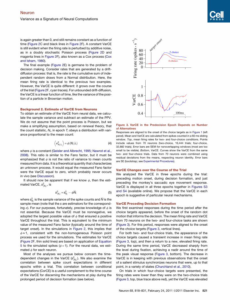
Figure 3. VarCE in the Predecision Epoch Depends on Number
of Alternatives
Responses are aligned to the onset of the choice targets as in Figure 1 (left
panel). Mean and VarCE are calculated from spikes counted in a 60 ms sliding
window. Top, mean firing rates for two- and four-choice conditions. Points
include values from 70 neurons (two-choice, 16,444 trials; four-choice,
32,882 trials). Error bars are SEM for nonoverlapping windows (most are too
small to be visible). Bottom, VarCE. Curves show the VarCE from the same
two- and four-choice trials. Data from 70 neurons were combined using
residual deviations from the means, respecting neuron identity. Error bars
are SE (bootstrap; see Experimental Procedures).
Background 2. Estimate of VarCE from NeuronsTo obtain an estimate of the VarCE from neural data, we calcu-
late the sample variance and subtract an estimate of the PPV.
We do not assume that the point process is Poisson, but we
make a simplifying assumption, based on renewal theory, that
the count statistic, Ni, in epoch Ti obeys a distribution with vari-
ance proportional to the mean count:
Ds2Ni jli
E=fhNijlii (4)
where f is a constant (Geisler and Albrecht, 1995; Nawrot et al.,
2008). This ratio is similar to the Fano factor, but it must be
emphasized that f is not the ratio of variance to mean counts
measured fromdata. It is a theoretical quantity that characterizes
an unknown process. It would equal the measured Fano factor
were the VarCE equal to zero, which probably never occurs
in vivo (see Discussion).
It should now be apparent that if we know f, then the esti-
mated VarCE, s2hNii, is
s2hNii = s2Ni� fNi (5)
where s2Niis the sample variance of the spike counts and N is the
sample mean (note that the s are estimators for the correspond-
ing s). For our purposes, fortunately, precise knowledge of f is
not essential. Because the VarCE must be nonnegative, we
adopted the largest possible value of f that ensured a positive
VarCE throughout the trial. This is equivalent to the minimum
value of the measured Fano factor (typically around the time of
target onset). In the simulations in Figure 2, this implies that
fz1, consistent with the non-homogeneous Poisson point
process we used for the simulations. The estimates for VarCE
(Figure 2F, thin solid lines) are based on application of Equation
5 to the simulated spikes (f= 1). For the neural data, we esti-
mated f for each neuron.
Most of the analyses we pursue below concern the time-
dependent changes in the VarCE (s2hNii). We also examine the
correlation between spike count expectations in different
epochs within a trial. This correlation between conditional
expectations (CorCE) is a useful complement to the time course
of the VarCE for discerning the mechanisms at play during the
prolonged period of decision formation (see below).
VarCE Changes over the Course of the TrialWe analyzed the VarCE in three epochs during the trial:
preceding motion onset, during decision formation, and just
preceding the monkey’s saccadic eye movement response.
VarCE is displayed in all three epochs together in Figures S3
and S4 (available online). We propose that the VarCE in each
epoch is suggestive of particular neural mechanisms.
VarCE Preceding Decision FormationWe first examined responses during the time period after the
choice targets appeared, before the onset of the random dot
motion that informs the decision. The mean firing rate and VarCE
from 70 neurons on the two- and four-choice tasks are shown
(Figure 3). For this period, responses were aligned to the onset
of the choice targets (Figure 3, vertical lines).
For both two- and four-choice trials, the appearance of the
choice targets caused a transient increase in mean firing rate
(Figure 3, top), and then a return to a new, elevated firing rate.
During the same time period, VarCE decreased sharply from
the level during fixation, achieving a nadir around the time of
the peak visual response (Figure 3, bottom). The decrease in
VarCE is in keeping with previous observations that the onset
of a salient stimulus synchronizes neurons that were, up to that
point, in a variety of states (Churchland et al., 2010).
On trials in which four-choice targets were presented, the
firing rates were lower than they were on the two-choice trials
(Figure 3, top, blue trace above red), yet the VarCE was elevated
Neuron 69, 818–831, February 24, 2011 ª2011 Elsevier Inc. 821
A B C D
E
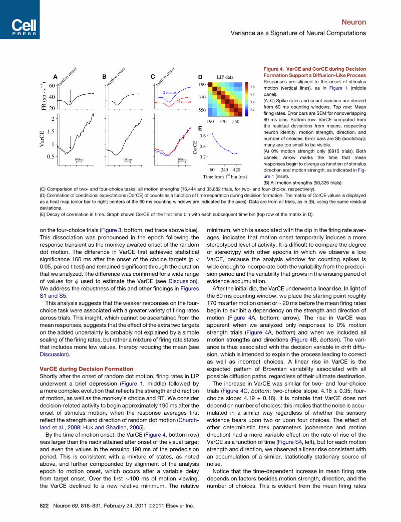
Figure 4. VarCE and CorCE during Decision
Formation Support aDiffusion-Like Process
Responses are aligned to the onset of stimulus
motion (vertical lines), as in Figure 1 (middle
panel).
(A–C) Spike rates and count variance are derived
from 60 ms counting windows. Top row: Mean
firing rates. Error bars are SEM for nonoverlapping
60 ms bins. Bottom row: VarCE computed from
the residual deviations from means, respecting
neuron identity, motion strength, direction, and
number of choices. Error bars are SE (bootstrap);
many are too small to be visible.
(A) 0% motion strength only (8815 trials). Both
panels: Arrow marks the time that mean
responses begin to diverge as function of stimulus
direction and motion strength, as indicated in Fig-
ure 1 (inset).
(B) All motion strengths (50,326 trials).
(C) Comparison of two- and four-choice tasks; all motion strengths (16,444 and 33,882 trials, for two- and four-choice, respectively).
(D) Correlation of conditional expectations (CorCE) of counts as a function of time separation during decision formation. The matrix of CorCE values is displayed
as a heat map (color bar to right; centers of the 60 ms counting windows are indicated by the axes). Data are from all trials, as in (B), using the same residual
deviations.
(E) Decay of correlation in time. Graph shows CorCE of the first time bin with each subsequent time bin (top row of the matrix in D).
Neuron
Variance as a Signature of Neural Computations
on the four-choice trials (Figure 3, bottom, red trace above blue).
This dissociation was pronounced in the epoch following the
response transient as the monkey awaited onset of the random
dot motion. The difference in VarCE first achieved statistical
significance 160 ms after the onset of the choice targets (p <
0.05, paired t test) and remained significant through the duration
that we analyzed. The difference was confirmed for a wide range
of values for f used to estimate the VarCE (see Discussion).
We address the robustness of this and other findings in Figures
S1 and S5.
This analysis suggests that the weaker responses on the four-
choice task were associated with a greater variety of firing rates
across trials. This insight, which cannot be ascertained from the
mean responses, suggests that the effect of the extra two targets
on the added uncertainty is probably not explained by a simple
scaling of the firing rates, but rather a mixture of firing rate states
that includes more low values, thereby reducing the mean (see
Discussion).
VarCE during Decision FormationShortly after the onset of random dot motion, firing rates in LIP
underwent a brief depression (Figure 1, middle) followed by
amore complex evolution that reflects the strength and direction
of motion, as well as the monkey’s choice and RT. We consider
decision-related activity to begin approximately 190 ms after the
onset of stimulus motion, when the response averages first
reflect the strength and direction of random dot motion (Church-
land et al., 2008; Huk and Shadlen, 2005).
By the time of motion onset, the VarCE (Figure 4, bottom row)
was larger than the nadir attained after onset of the visual target
and even the values in the ensuing 190 ms of the predecision
period. This is consistent with a mixture of states, as noted
above, and further compounded by alignment of the analysis
epoch to motion onset, which occurs after a variable delay
from target onset. Over the first �100 ms of motion viewing,
the VarCE declined to a new relative minimum. The relative
822 Neuron 69, 818–831, February 24, 2011 ª2011 Elsevier Inc.
minimum, which is associated with the dip in the firing rate aver-
ages, indicates that motion onset temporarily induces a more
stereotyped level of activity. It is difficult to compare the degree
of stereotypy with other epochs in which we observe a low
VarCE, because the analysis window for counting spikes is
wide enough to incorporate both the variability from the predeci-
sion period and the variability that grows in the ensuing period of
evidence accumulation.
After the initial dip, the VarCE underwent a linear rise. In light of
the 60 ms counting window, we place the starting point roughly
170ms after motion onset or�20ms before themean firing rates
begin to exhibit a dependency on the strength and direction of
motion (Figure 4A, bottom; arrow). The rise in VarCE was
apparent when we analyzed only responses to 0% motion
strength trials (Figure 4A, bottom) and when we included all
motion strengths and directions (Figure 4B, bottom). The vari-
ance is thus associated with the decision variable in drift diffu-
sion, which is intended to explain the process leading to correct
as well as incorrect choices. A linear rise in VarCE is the
expected pattern of Brownian variability associated with all
possible diffusion paths, regardless of their ultimate destination.
The increase in VarCE was similar for two- and four-choice
trials (Figure 4C, bottom; two-choice slope: 4.16 ± 0.35; four-
choice slope: 4.19 ± 0.16). It is notable that VarCE does not
depend on number of choices: this implies that the noise is accu-
mulated in a similar way regardless of whether the sensory
evidence bears upon two or upon four choices. The effect of
other deterministic task parameters (coherence and motion
direction) had a more variable effect on the rate of rise of the
VarCE as a function of time (Figure S4, left), but for each motion
strength and direction, we observed a linear rise consistent with
an accumulation of a similar, statistically stationary source of
noise.
Notice that the time-dependent increase in mean firing rate
depends on factors besides motion strength, direction, and the
number of choices. This is evident from the mean firing rates
A B C
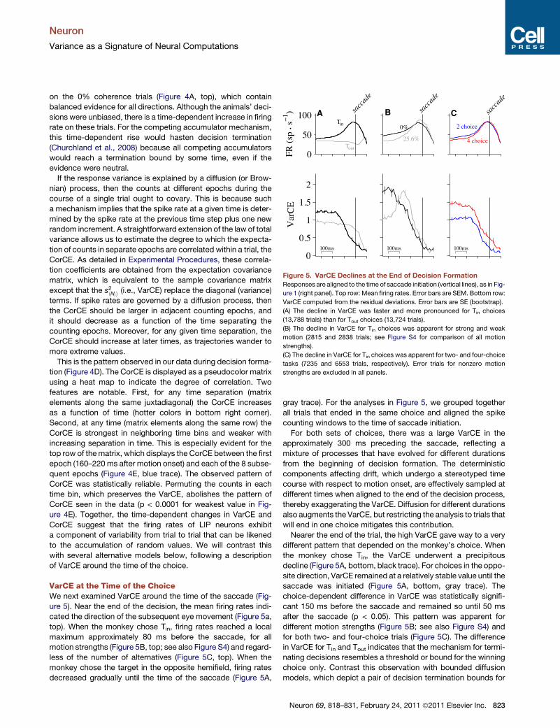
Figure 5. VarCE Declines at the End of Decision FormationResponses are aligned to the time of saccade initiation (vertical lines), as in Fig-
ure 1 (right panel). Top row: Mean firing rates. Error bars are SEM. Bottom row:
VarCE computed from the residual deviations. Error bars are SE (bootstrap).
(A) The decline in VarCE was faster and more pronounced for Tin choices
(13,788 trials) than for Tout choices (13,724 trials).
(B) The decline in VarCE for Tin choices was apparent for strong and weak
motion (2815 and 2838 trials; see Figure S4 for comparison of all motion
strengths).
(C) The decline in VarCE for Tin choices was apparent for two- and four-choice
tasks (7235 and 6553 trials, respectively). Error trials for nonzero motion
strengths are excluded in all panels.
Neuron
Variance as a Signature of Neural Computations
on the 0% coherence trials (Figure 4A, top), which contain
balanced evidence for all directions. Although the animals’ deci-
sions were unbiased, there is a time-dependent increase in firing
rate on these trials. For the competing accumulator mechanism,
this time-dependent rise would hasten decision termination
(Churchland et al., 2008) because all competing accumulators
would reach a termination bound by some time, even if the
evidence were neutral.
If the response variance is explained by a diffusion (or Brow-
nian) process, then the counts at different epochs during the
course of a single trial ought to covary. This is because such
a mechanism implies that the spike rate at a given time is deter-
mined by the spike rate at the previous time step plus one new
random increment. A straightforward extension of the law of total
variance allows us to estimate the degree to which the expecta-
tion of counts in separate epochs are correlated within a trial, the
CorCE. As detailed in Experimental Procedures, these correla-
tion coefficients are obtained from the expectation covariance
matrix, which is equivalent to the sample covariance matrix
except that the s2hNii (i.e., VarCE) replace the diagonal (variance)
terms. If spike rates are governed by a diffusion process, then
the CorCE should be larger in adjacent counting epochs, and
it should decrease as a function of the time separating the
counting epochs. Moreover, for any given time separation, the
CorCE should increase at later times, as trajectories wander to
more extreme values.
This is the pattern observed in our data during decision forma-
tion (Figure 4D). The CorCE is displayed as a pseudocolor matrix
using a heat map to indicate the degree of correlation. Two
features are notable. First, for any time separation (matrix
elements along the same juxtadiagonal) the CorCE increases
as a function of time (hotter colors in bottom right corner).
Second, at any time (matrix elements along the same row) the
CorCE is strongest in neighboring time bins and weaker with
increasing separation in time. This is especially evident for the
top row of thematrix, which displays the CorCE between the first
epoch (160–220 ms after motion onset) and each of the 8 subse-
quent epochs (Figure 4E, blue trace). The observed pattern of
CorCE was statistically reliable. Permuting the counts in each
time bin, which preserves the VarCE, abolishes the pattern of
CorCE seen in the data (p < 0.0001 for weakest value in Fig-
ure 4E). Together, the time-dependent changes in VarCE and
CorCE suggest that the firing rates of LIP neurons exhibit
a component of variability from trial to trial that can be likened
to the accumulation of random values. We will contrast this
with several alternative models below, following a description
of VarCE around the time of the choice.
VarCE at the Time of the ChoiceWe next examined VarCE around the time of the saccade (Fig-
ure 5). Near the end of the decision, the mean firing rates indi-
cated the direction of the subsequent eye movement (Figure 5a,
top). When the monkey chose Tin, firing rates reached a local
maximum approximately 80 ms before the saccade, for all
motion strengths (Figure 5B, top; see also Figure S4) and regard-
less of the number of alternatives (Figure 5C, top). When the
monkey chose the target in the opposite hemifield, firing rates
decreased gradually until the time of the saccade (Figure 5A,
gray trace). For the analyses in Figure 5, we grouped together
all trials that ended in the same choice and aligned the spike
counting windows to the time of saccade initiation.
For both sets of choices, there was a large VarCE in the
approximately 300 ms preceding the saccade, reflecting a
mixture of processes that have evolved for different durations
from the beginning of decision formation. The deterministic
components affecting drift, which undergo a stereotyped time
course with respect to motion onset, are effectively sampled at
different times when aligned to the end of the decision process,
thereby exaggerating the VarCE. Diffusion for different durations
also augments the VarCE, but restricting the analysis to trials that
will end in one choice mitigates this contribution.
Nearer the end of the trial, the high VarCE gave way to a very
different pattern that depended on the monkey’s choice. When
the monkey chose Tin, the VarCE underwent a precipitous
decline (Figure 5A, bottom, black trace). For choices in the oppo-
site direction, VarCE remained at a relatively stable value until the
saccade was initiated (Figure 5A, bottom, gray trace). The
choice-dependent difference in VarCE was statistically signifi-
cant 150 ms before the saccade and remained so until 50 ms
after the saccade (p < 0.05). This pattern was apparent for
different motion strengths (Figure 5B; see also Figure S4) and
for both two- and four-choice trials (Figure 5C). The difference
in VarCE for Tin and Tout indicates that the mechanism for termi-
nating decisions resembles a threshold or bound for the winning
choice only. Contrast this observation with bounded diffusion
models, which depict a pair of decision termination bounds for
Neuron 69, 818–831, February 24, 2011 ª2011 Elsevier Inc. 823
A B C D E
F G H I J
P Q R S T
K L M N O
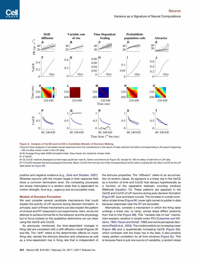
Figure 6. Analysis of VarCE and CorCE in Candidate Models of Decision Making
Columns show analyses of simulated neural responses from five mechanisms in the epoch of early decision formation (corresponding to the epoch beginning
�190 ms after motion onset in the LIP data).
(A–E) Average firing rates (5000 simulated trials). Gray traces: ten randomly chosen trials.
(F–J) VarCE.
(K–O) CorCE matrices displayed as heat maps (scale bar near K). Same conventions as Figure 4D, except for 190 ms delay of start time in LIP data.
(P–T) CorCE between first and subsequent time bins. Black: CorCE from the top row of the corresponding CorCEmatrix in panels (K)–(O). Blue: CorCE for the LIP
data (same as Figure 4E).
Neuron
Variance as a Signature of Neural Computations
positive and negative evidence (e.g., Gold and Shadlen, 2007).
Whereas neurons with the chosen target in their response field
show a common termination level, the competing processes
are simply interrupted in a random state that is dependent on
motion strength, time (e.g., urgency) and accumulated noise.
Models of Decision FormationWe next consider several candidate mechanisms that could
explain the activity of LIP neurons during decision formation. In
principle, each of thesemechanisms can also explain the pattern
of choices and RTmeasured in our experiments. Here, we do not
attempt to achieve formal fits to the behavior and the physiology
but to focus instead on the qualitative distinctions we can draw
using the VarCE and CorCE.
As previously mentioned, the time-dependent changes in
firing rate are consistent with a drift diffusion model (Figures 2E
and 6A). The ‘‘drift’’ refers to the deterministic effects on mean
firing rate, namely the stimulus direction and coherence as well
as a time-dependent rise in firing rate that is independent of
824 Neuron 69, 818–831, February 24, 2011 ª2011 Elsevier Inc.
the stimulus properties. The ‘‘diffusion’’ refers to an accumula-
tion of random values. Its signature is a linear rise in the VarCE
as a function of time and CorCE that decays hyperbolically as
a function of the separation between counting windows
(Methods Equation 10). These patterns are apparent in the
VarCE and CorCE of LIP neurons during early decision formation
(Figure 6P, blue and black curves). The increase in overall corre-
lation at late times (Figure 6K, lower right corner) is subtler in data
because responses near the RT are excluded.
Alternatively, consider a mechanism in which the firing rates
undergo a linear rise, or ramp, whose slope differs randomly
from trial to trial (Figure 6B). This ‘‘variable rate of rise’’ mecha-
nism explains variation in simple motor RTs (Carpenter and Wil-
liams, 1995; Hanes and Schall, 1996) and some perceptual deci-
sions (Reddi et al., 2003). Themodel predicts an increasingmean
(Figure 6B) and a quadratically increasing VarCE (Figure 6G),
which contrasts with the linear rise in the data. It also predicts
nearly perfect correlation for all time windows (Figure 6L). This
is because there is just one source of variability, a random slope
A B
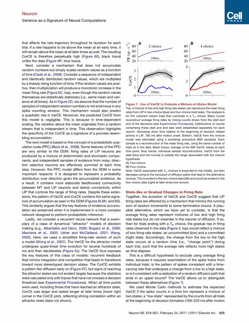
Figure 7. Use of VarCE to Evaluate a Mixture-of-States Model
Top, a mixture of low and high firing rate states can reproduce the mean firing
rates from LIP in two-choice (blue) and four-choice (red) tasks. The analysis is
for 0% coherent motion trials that culminate in a Tin choice. Black curves
reconstruct average firing rates by mixing counts drawn from the start and
end of the decisions (see Experimental Procedures). Distributions of counts
comprising these start and end sets were established separately for each
neuron. Abscissae show time relative to the beginning of decision related
activity in LIP, 190 ms after motion onset. Bottom, VarCE from the mixture
model was estimated using a bootstrap procedure (600 samples). Each
sample is a reconstruction of the mean firing rate, using the same number of
trials as in the data. Black traces: average of the 600 VarCE values at each
time point. Gray traces: individual sample reconstructions. VarCE from the
data (blue and red curves) is outside the range associated with the mixture
hypothesis.
(A) Two-choice.
(B) Four-choice.
Note: VarCE associated with Tin choices is expected to rise initially, but then
decrease owing to the exclusion of diffusion paths that lead to the alternative
choices. This is evident in the two-choice data (left) andwould be evident in the
four-choice data (right) at later times (not shown).
Neuron
Variance as a Signature of Neural Computations
that affects the rate trajectory throughout its duration for each
trial. If a rate happens to be above the mean at an early time, it
will remain above themean at all later times as well. The resulting
CorCE is therefore perpetually high (Figure 6Q, black trace)
unlike the data (Figure 6P, blue trace).
Next, consider a mechanism that does not accumulate
random numbers but simply scales random values as a function
of time (Cisek et al., 2009). Consider a sequence of independent
and identically distributed random values, which are multiplied
by a linearly rising function of time. If the random values are posi-
tive, then multiplication will produce a monotonic increase in the
mean firing rate (Figure 6C, top), even though the random values
themselves are statistically stationary (i.e., same mean and vari-
ance at all times). As in Figure 2D, we assume that the number of
samples of independent randomnumbers is not enormous in any
spike counting window. This mechanism would also predict
a quadratic rise in VarCE. Moreover, the predicted CorCE from
this model is negligible. This is because in time-dependent
scaling, the variation about the mean originates from a random
stream that is independent in time. This observation highlights
the specificity of the CorCE as a signature of a process resem-
bling accumulation.
The next model is based on the concept of a probabilistic pop-
ulation code (PPC) (Beck et al., 2008). Some features of the PPC
are very similar to the DDM: firing rates of LIP neurons are
produced by a mixture of deterministic and stochastic compo-
nents, and independent samples of evidence from noisy, direc-
tion selective neurons are effectively summed at each time
step. However, the PPC model differs from the DDM in some
important respects: it is designed to represent a probability
distribution over direction given the accumulated evidence. As
a result, it contains more elaborate feedforward connectivity
between MT and LIP neurons and lateral connectivity within
LIP that controls the range of firing rates. Despite these exten-
sions, the pattern of VarCE and CorCE contains the same signa-
ture of accumulation as seen in the DDM (Figures 6I,6N, and 6S).
This similarity argues that the key features of evidence accumu-
lation are preserved when it is implemented in a more complex
network designed to perform probabilistic inference.
Lastly, we consider a recurrent neural network that is exem-
plary of a class of dynamical ‘‘attractor’’ models of decision
making (e.g., Albantakis and Deco, 2009; Bogacz et al., 2006;
Machens et al., 2005; Usher and McClelland, 2001; Wang,
2002). Here, we used a simplified firing-rate version of such
a model (Wong et al., 2007). The VarCE for the attractor model
undergoes quasi-linear time evolution for several hundreds of
ms and then decelerates (Figure 6J). The VarCE thus exposes
the key features of this class of models: recurrent feedback
that mimics integration and competition that leads to transitions
toward more stereotyped decision states. The CorCE exhibits
a pattern like diffusion early on (Figure 6T), but signs of reaching
the attractor states are not evident largely because the statistics
were calculated onlywith traces that have not crossed a decision
threshold (see Experimental Procedures). When all time points
were used, including those that have reached an attractor state,
CorCE was larger and lasted longer at later times (lower right
corner in the CorCE plot), reflecting strong correlation within an
attractor state (data not shown).
State-like or Gradual Changes in Firing RateTogether, the evolution of VarCE and CorCE suggest that LIP
firing rates are affected by a mechanism that mimics the running
sum of random increments to some termination bound. A plau-
sible alternative, which we have yet to consider, is that the
average firing rates represent mixtures of low and high firing
rate states but do not meander in the manner of diffusion. If so,
then for trials ending with a Tin choice, the gradual rise in firing
rates observed in the data (Figure 4, top) would reflect a mixture
of two firing rate states: an uncommitted (low) and a committed
(high) state. Accordingly, the change from the low to the high
state occurs at a random time (i.e., ‘‘change point’’) during
each trial, such that the average rate reflects more high states
as time elapses.
This is a difficult hypothesis to exclude using average firing
rates, because it requires examination of the spike trains from
individual trials: is the pattern of spikes consistent with a time-
varying rate that undergoes a change from a low to a high state,
or is it consistent with a realization of a randomdiffusion path that
ends in an upper bound? The VarCE allows us to distinguish
between these alternatives (Figure 7).
We used Monte Carlo methods to estimate the expected
VarCE if the spike counts in a time bin represent a mixture of
two states: a ‘‘low state’’ represented by the counts from all trials
at the beginning of decision formation (160–220 ms after motion
Neuron 69, 818–831, February 24, 2011 ª2011 Elsevier Inc. 825
Neuron
Variance as a Signature of Neural Computations
onset) and a ‘‘high state’’ represented by the counts from all trials
at the end of decisions for Tin (110–50 ms before saccade initia-
tion). Unlike previous analyses, we include only trials in which the
monkey chose Tin. We reconstituted the observed firing rate
averages using random mixtures of the sets of counts
comprising the low and high states (Figure 7, top; black traces;
see Experimental Procedures). The VarCE for the mixture in
the earliest time bins are indistinguishable from the data (colored
traces), because themixtures are comprisedmainly from the low
state. However, as time elapses, the mixture of low and high
states required to produce the observed mean would be associ-
ated with a larger VarCE (Figure 7, bottom; black traces).
The analysis leads us to reject the mixture (change point)
model for trials ending in Tin choices (p < 0.002 for both two-
and four-choice). This conclusion is further supported by an
analysis of the CorCE, which is predicted to be weaker under
the mixture model (data not shown, p < 0.001; bootstrap, Exper-
imental Procedures). We cannot perform such analyses on Toutchoices because, as shown above, there is no evidence for
a stereotyped state at the termination of these trials. Finally,
we note that by restricting the analysis to Tin choices, the VarCE
is not the one associated with diffusion (which must consider
paths leading to all choices). The VarCE for Tin choices would
ultimately decline as the responses approach the stereotyped
high state before the saccade. There is a hint of this decline in
Figure 7A (bottom).
DISCUSSION
Neural variability is frequently regarded as a nuisance: the highly
variable discharge of cortical neurons necessitates collecting
multiple repetitions of the same stimulus to generate a reliable
estimate of the underlying mean firing rate, and it necessitates
populations of neurons to transmit a reliable estimate of rate
on one trial. However, variance itself, especially its time course,
can be diagnostic of neural computations. Here too, the variable
discharge of neurons is a nuisance, as it obscures the aspect of
variance that is potentially diagnostic, the variance of the quan-
tity that the neuron is supposed to represent. We have intro-
duced a measure that allows us to look past one component
of variance, the one associatedwith spiking, to gain insight about
neural computations during decision making.
Our main innovation is to depict the measured variance of
spike counts as a reflection of a doubly stochastic process:
a PPV associated with an idealized stochastic point process
that would produce a random number of spikes even if some
‘‘intensity command’’ were identical on every repetition and
a VarCE that describes the variance of that intensity command.
This decomposition is a straightforward application of the law
of total variance. We emphasize that the decomposition is
a conceptual contrivance that does not conform to neurophysi-
ological processes (e.g., synaptic integration and spike genera-
tion), at least not directly. Yet, it has the same intuitive appeal as
the peristimulus time histogram (PSTH): it is a way of looking past
the variability inherent in spike trains to infer the underlying
computation. The PSTH recovers the mean intensity as a func-
tion of time, whereas the VarCE and CorCE recover properties
of variance of that intensity across repetitions.
826 Neuron 69, 818–831, February 24, 2011 ª2011 Elsevier Inc.
Comparison to Other Variance MeasuresUnlike the measured sample variance, the VarCE is intended to
expose that component of variation that is tied to neural
computation. By suppressing a component of the variance
explained by irregular spiking, it reveals the trial-to-trial variance
in the underlying rates. A larger VarCE implies greater heteroge-
neity of states across trials, and a linear increase in VarCE as
a function of time is a hallmark of a diffusion or random walk
process. The total variance cannot reveal such processes
because all increases in firing rate are associatedwith larger total
variance in cortex.
To a large extent, the ratio of the variance-to-mean spike
count (the Fano factor) achieves something similar to VarCE,
because it normalizes the sample variance to the mean count.
Both measures embrace the simplifying approximation that
would liken spike trains to rate-modulated renewal processes:
their intervals are independent and identically distributed once
time is scaled to achieve the modulation of rate (Nawrot et al.,
2008). In general, the Fano factor and VarCE ought to be qualita-
tively consistent (but see, Figure S2A). Indeed most of our
conclusions would be supported by an analysis of the Fano
factor (Figures S2B–S2D).
Themain advantage of VarCE is that it is principled. It captures
the variance of the rates, actually the integrated rate across the
counting window, from trial to trial. Therefore, it has a natural
link to standard dispersion measures (e.g., regression sum of
squares as opposed to residual sum of squares, or the variance
of the sum of independent random variables, as in diffusion). It is
also a necessary first step in the calculation of the CorCE, which
can be a highly diagnostic tool.
The main alternative to the CorCE is the spike autocorrelation
function. The latter conflates variation in rate with variation in
interspike interval, whereas CorCE isolates the former. Although
it is beyond the scope of the present exercise, we anticipate that
the CorCE could be adopted to better clarify the spike autocor-
relation function in situations when rates undergo trial-to-trial
variation. An extension to the cross correlation of firing rates
(or spike cross-correlogram) is another potentially useful exten-
sion, especially when the rate is changing in time and from trial
to trial (Aertsen et al., 1989; Vaadia et al., 1995).
Drawbacks of VarCE and CorCESince the VarCE is estimated by subtracting the PPV from the
measured spike count variance, any uncertainty about the nature
and magnitude of the PPV invites concerns about the validity of
the VarCE and CorCE, and therefore about the conclusions we
draw from these estimates. We have embraced three assump-
tions, which are incorrect but largely innocuous.
The first assumption is that PPV is proportional to the mean
count. This holds if spike trains are properly characterized as
rate-modulated renewal processes (Nawrot et al., 2008). For
such a process, the variance of counts in an epoch is propor-
tional to the mean. This is the inspiration for the expression for
the PPV in Equation 4. We recognize that neural spike trains
do not conform exactly to this characterization. For example,
when the firing rate changes, the refractory period does not scale
in the way that the intervals do. Other violations of the renewal-
like assumption are characterized in Teich et al. (1997), although
Neuron
Variance as a Signature of Neural Computations
we suspect some are simply manifestations of VarCE and less
exotic than these authors propose. For example, a change in
Fano factor with window duration might be explained by
mixtures or diffusion.
Important as they are, these caveats matter only to the degree
that the PPV would be characterized erroneously as a value
proportional to mean count, but this approximation appears
secure. Only approximate conformity to the ‘‘rate-modulated
renewal’’ assumption is required, and for this there is ample
support (Nawrot et al., 2008). There is an approximately linear
relationship between the mean and variance of the spike counts
for neurons in several cortical areas for repetitions of identical
stimuli (Britten et al., 1993; Churchland et al., 2006; Geisler and
Albrecht, 1995;McAdams andMaunsell, 1999). These are condi-
tions in which we would expect the VarCE to be minimal, and the
same holds for LIP neurons when rates are relatively stationary,
as in the delay period preceding a saccade to one target or
during the late predecision period (cf. Maimon and Assad,
2009). These observations provide empirical support for the
proportional relationship, PPV =fN, even if the magnitude of f
is unresolved.
The second assumption is that f is fixed for the neuron; it does
not depend on firing rate or state. This is unlikely to be true in all
instances, and it could lead to inaccurate estimates of VarCE.
For example, conditions favoring bursting in one epoch might
affect our estimate of f but fail to apply in other epochs, when
the neuron is not bursting. That said, the observation of a roughly
fixed ratio of variance to mean spike count and its near indepen-
dence from conditions affecting the mean firing rate, such as
motion strength, contrast, and attentional state (Britten et al.,
1993; Geisler et al., 2001; McAdams and Maunsell, 1999;
Tolhurst et al., 1983), imply that f is unlikely to vary systemati-
cally as a function of firing rate. Were f a function of firing rate,
then, to achieve a constant ratio of variance to mean count,
the PPV and VarCE would necessarily contribute different
proportions of the total variance when the firing rate changes.
For example, if higher firing rates were associated with smaller
f (and hence a smaller PPV), then the constant ratio of variance
to mean count could only be achieved if the decrease in PPV
were offset by a concomitant increase in VarCE. This implies
that the neuron’s spike discharge is less variable at higher rates,
whereas the spikes comprising the input to the neuron are more
variable. This seems highly implausible.
We favor a more consistent and parsimonious account of
inputs and outputs: when a neuron is pushed to respond at
a higher rate, both the variance of its inputs and the variance
associated with its own spiking increase proportionately and
thus preserve a consistent ratio of variance to mean spike count
at low and high firing rates (Shadlen and Newsome, 1998). When
this ratio changes, it is probably a reflection of a change in VarCE
such as when conditions vary from trial to trial (i.e., mixture of
states).
The third assumption is that f can be approximated from
neural data. This is truly suspect. Even if our own application of
an upper bound is valid, it is unlikely to be helpful in data sets
that do not furnish a plausible nadir in the measured Fano factor.
Nonetheless, several practical heuristics serve to constrain esti-
mates of f. The VarCE must be nonnegative and less than the
measured variance. Indeed it is unlikely that the VarCE is ever
equal to zero in vivo, even under stable conditions in which vari-
ation in the ‘‘intensity command’’ ought to be minimal, because
even highly stereotyped conditions do not remove all variability
in synaptic inputs to neurons. This alone indicates that f is less
than the measured Fano factor. Similarly, the CorCE, which
depends on the VarCE, must fall between ± 1. This constrains
f to lower values.
Finally, theoretical considerations suggest an upper bound for
f, independent of the measured Fano factor. A Poisson process
with refractoriness ensures f < 1 (Berry and Meister, 1998; Keat
et al., 2001). For example, a 1.5 ms refractory period yields
fz0:8 over a range of firing rates commonly encountered in
cortex. For cortical neurons that operate in a high input regimen
with balance of excitation and inhibition, a good choice for f is in
the range 0.4 to 0.7 (Nawrot et al., 2008; Shadlen and Newsome,
1998). Together, these heuristics might be applied judiciously
in situations when themeasured variance or Fano factor appears
stationary as a function of time. Thus when a physiologist
measures a Fano factor equal to 1.5, it may be reasonable to
speculate that at least half of the measured variance is attributed
to VarCE.
The above concerns reinforce the point that VarCE is useful
mainly to compare responses when the neuron is likely to be in
the same state, as when we compare responses in the predeci-
sion epoch in the two- and four-choice tasks, or when we
examine the time course of VarCE during decision formation.
We must exercise caution, however, when comparing the VarCE
after target onset and before the saccade. In general, any
conclusions that rest on the magnitude of VarCE and CorCE
should be tested for robustness against variation in f.
Importantly, the main conclusions of our study do not depend
on precise knowledge of f (Figure S1). The linear rise in VarCE
during decision formation is difficult to explain away, because
it would require f to change in just the right way to cancel the
slope in Figure 4, bottom. Nevertheless, to evaluate this further,
we repeated our analysis of the spike count variance using
subsets of the data matched for firing rates (Churchland et al.,
2010) (Figure S5). These analyses provide reassurance that the
time-dependent changes in VarCE and CorCE did not result
from a misestimate of f or because f changed as a result of
the time-varying firing rate.
VarCE during the Predecision Period, Decision
Formation, and Near the Saccade
Previous analyses of the neural responses in LIP combined with
analyses of choice and RT support a bounded integration mech-
anism for decision making. The analyses of the VarCE and
CorCE, presented here, lend independent support for this idea
and expose new features of the neural computations that
underlie the decision process: amixture of firing rates associated
with the predecision period, time integration of a stochastic vari-
able during decision formation, and a threshold for terminating
the decision.
During the predecision interval, we observed a higher VarCE
on a four-choice version of the task compared with a two-choice
version of the task. This observation suggests that the lower
average firing rate on the four-choice task belies a broader
mixture of firing rates from trial to trial, most of which are lower
Neuron 69, 818–831, February 24, 2011 ª2011 Elsevier Inc. 827
Neuron
Variance as a Signature of Neural Computations
in the four-choice task. The lower average rate is probably not
explained by amechanism that invokes less excitation or greater
suppression on all trials, owing perhaps to greater uncertainty
(Basso and Wurtz, 1998), or normalization (Tolhurst and Heeger,
1997), or surround inhibition (Balan et al., 2008). Each of these
mechanisms would simply scale the firing rate depending on
the number of choices. They explain the lower firing rate on the
four-choice task, but they cannot explain the higher VarCE
without additional assumptions.
During decision formation, the analysis of VarCE and CorCE
provide direct support for stochastic accumulation by showing
that the firing rates of LIP neurons are effectively sample-trajec-
tories described by drift-diffusion. By perturbing the background
of random dot motion displays, Huk and Shadlen (2005) demon-
strated that LIP neurons represent the integral of motion
evidence in the display, but thesemeasurements did not demon-
strate that spike trains from individual trials represent realizations
of random walk or diffusion-like processes. An increase in vari-
ability during evidence accumulation is predicted by models of
integration (Miller and Wang, 2006) but has not been demon-
strated experimentally until now.
The pattern of VarCE and CorCE help to exclude several
important alternatives to stochastic accumulation. For example
a gradual shift in attention toward the choice target that simply
follows a particular time course will not explain the increase in
VarCE (Gottlieb and Balan, 2010). Similarly a change in the
amplitude, or gain, of a signal (time-dependent scaling, Figure 6,
middle column) would not explain the pattern of CorCE that we
observed during decision formation. A variable rate-of-rise
model (Figure 6, second column), where there is just one source
of variability, a random slope that affects the rate trajectory for
each trial, is also incompatible with the CorCE that we observed.
The present exercise renders as unlikely any mechanism that
lacks a Brownian component even if it gives rise to similar
time-dependent evolution in firing rates.
The increase in VarCE that we report during decision
formation differs from the pattern of variability that is apparent
in tasks that do not rely on the accumulation of evidence. For
example, in dorsal premotor cortex, neural variability decreases
gradually until the monkey’s movement, sometimes over
a period as long as 400 ms (Churchland et al., 2006). Responses
in LIP on a probabilistic reward task likewise decrease following
the onset of a salient stimulus (Churchland et al., 2010). In light
of the present work, our interpretation is that presenting a
stimulus establishes experimental control and thus replaces
a mixture of states across trials with greater consistency. We
observed a similar decrease in variability in our data, following
the presentation of choice targets, and again following the
onset of random dot motion (Figure 3) before the period of
evidence accumulation. By contrast, during decision formation,
the VarCE underwent a dramatic linear rise (Figure 4, bottom)
consistent with the accumulation over time of random samples
of evidence.
These observations argue that the variability of neural
responses, rather than simply hindering one’s ability to estimate
the mean, can be exploited to constrain neural computations,
particularly those that cannot be discerned from measures of
average firing rate. This technique reveals that on decision-
828 Neuron 69, 818–831, February 24, 2011 ª2011 Elsevier Inc.
making tasks, LIP neurons reflect a mixture of states at the
beginning of the trial, accumulation of evidence during decision
formation, and a stereotyped level at decision end.
EXPERIMENTAL PROCEDURES
Behavior and Physiology
All behavioral and neural data were previously published (see Churchland
et al., 2008). In brief, after a variable fixation period, two or four peripheral
choice targets appeared to signal the direction alternatives on the trial. After
a random delay (250–800 ms), dynamic random dot motion was displayed in
a 5� diameter aperture centered at the fixation point. Task difficulty was
controlled by varying the percentage of coherently moving dots on each trial
(speed = 6�/s). The motion stimulus was extinguished when the monkey’s
gaze moved outside the fixation window, thereby marking the time of saccade
initiation. The data set consists of extracellular recordings from 70 well-iso-
lated neurons in area LIPv (Lewis and Van Essen, 2000).
Data Analysis
Estimation of Mean
We computed mean responses (Figure 1 and top panels in Figures 3–5) from
the spike counts in 60 ms counting windows (bins) over repetitions of trials
grouped by condition (motion strength, direction, etc.). We used this brief
counting window to facilitate examination of the response dynamics. Other
window sizes yielded qualitatively similar results. All references to time refer
to the midpoint of the counting window.
Estimation of Variance of the Conditional Expectation (VarCE)
We estimated the VarCE in the same time windows used to estimate themean.
VarCE is estimated from a list of counts by subtracting an estimate of the PPV
from the sample variance (Equation 5). Its units are spikes2. For each neuron,
we obtain an estimate of the PPV by finding the time window with the smallest
ratio of variance to mean (i.e., the Fano factor). Were VarCE = 0 in this epoch,
the measured variance would approximate the PPV. We take the Fano factor
from this epoch as an upper bound estimate of f for each neuron (median =
0.46, IQR = 0.23 to 0.70).
To enhance the power of most analyses, we combined data from several
conditions (e.g., motion strength, neuron, etc.) that did not share the same
mean count. To prevent this variation among the means from contributing to
the combined variance, we estimated the variance using the residuals, that
is, by subtracting from each sample count the mean for all trials sharing its
condition. For example, in early decision formation, a condition would
comprise all trials for one neuron that were obtained using the same motion
strength, direction, and number of choices.
The VarCE is then the variance of the union of residuals from all conditions,
zW, minus the weighted average of the PPV for the conditions:
s2hNi i =Var½zW� �XMi = 1
ni
nWfiNi (6)
where nW is the total number of samples across allM conditions, ni and Ni are
the number of samples and the mean count for the i th condition, respectively.
Values of fwere the same for all conditions for a neuron: the largest value that
ensures VarCE > 0 for that neuron over all conditions and epochs. Standard
error (SE) of s2hNii was estimated using a bootstrap procedure that preserved
the number of trials in each condition (SE is the sample standard deviation
from 200 samples). Similar results were obtained when we computed the
VarCE separately for each condition and then averaged the values.
We computed the Fano factor in a similar way:
FFhNi i =Var½zW�PMi = 1
ninW
Ni
(7)
using the same conventions as Equation 6. SEs were computed using a boot-
strap procedure.
The trial groupings that define a condition depend on the analysis. In the pre-
decision epoch (Figure 3), we computed residuals using means from all trials
from a neuron in either the two- or the four-choice condition. For early decision
Neuron
Variance as a Signature of Neural Computations
formation (Figure 4), we computed residuals using the means from each
neuron, motion strength, motion direction, and number of choice targets. In
this epoch, trials that ultimately led to any of the possible choices were
grouped together. Each trial contributed data so long as the time of saccade
initiation was at least 100 ms after the end of the bin (i.e., 130 ms after the
time displayed on the abscissa). Therefore, the numbers of trials contributing
to each point in Figure 4 changes over time. Points on the plots in Figure 4 indi-
cate times when at least 25% of the trials were still contributing to the average
(i.e., the RT for those trials was longer than the time point in question); varying
this cutoff did not have a major impact on the time-dependent rise. The same
time-dependent rise in VarCE was present when we restricted the analysis to
trials with an RT >700 ms and included all trials at each time point (data not
shown). For responses in the perisaccadic epoch, we computed residuals
using the means from each neuron, motion strength, motion direction, number
of choice targets, and choice. Note that the number of conditions contributing
to each epoch’s analysis varied considerably. For example, when comparing
two- and four-choice responses during the predecision period, all trials were
included. For the same comparison around the time of the saccade, by
contrast, trials that ended in a particular choice (i.e., Tin or Tout) were analyzed
separately. As a result, many fewer trials contributed to each group.
Temporal Correlations
The approach we use to estimate the VarCE extends naturally to pairwise
measurements. Just as VarCE lends insight into the variance of an observed
rate from trial to trial, the CorCE approximates the correlation between pairs
of rates at different times during a trial. In both cases, we measure a total vari-
ance or covariance and correct for a portion that is caused by the point
process. From the law of total covariance,
Cov½Ni ;Nj �= Cov½hNi jlii;�Nj
��lj��|fflfflfflfflfflfflfflfflfflfflfflfflfflfflfflfflffl{zfflfflfflfflfflfflfflfflfflfflfflfflfflfflfflfflffl}covariance of
conditional expectations
+�Cov½Ni ;Nj
��li ; lj��|fflfflfflfflfflfflfflfflfflfflfflfflfflfflffl{zfflfflfflfflfflfflfflfflfflfflfflfflfflfflffl}expectation of
conditional covariance
(8)
where the indices refer to epochs in time across the trial and theN and l terms
are spike counts and rates. As before, it is the first term on the right side of
equation that interests us. The second term is the PPV when i = j. When isj,
this term should be zero, because the variation associated with rendering
a rate into a point process ought to be independent in two epochs. This
reasoning is technically incorrect for adjacent bins because they share an in-
terspike interval, but we saw nearly identical effects when we used bins that
were separated by 30 ms (data not shown).
These considerations imply that the measured covariance is the covari-
ance of the conditional expectation for the nondiagonal terms of the
covariance matrix, and is simply the VarCE terms for the diagonal. The CorCE
is obtained by writing the covariance matrix of conditional expectations
(CovCE) as
0BB@
s2hN1i . r1mffiffiffiffiffiffiffiffiffiffiffiffiffiffiffiffiffiffiffis2hN1is
2hNmi
q« 1 «
r1mffiffiffiffiffiffiffiffiffiffiffiffiffiffiffiffiffiffiffis2hN1is
2hNmi
q/ s2hNm i
1CCA=
0@ VarCE1 . Cov½N1;Nm�
« 1 «Cov½Nm;N1� / VarCEm
1A
(9)
and solving for the rij , wherem is the number of epochs. The right side of Equa-
tion 9 should be checked to ensure that CovCE is positive definite, and, if it is
not, then f must be lowered until it is. This procedure was not essential in our
applications only because f was determined from responses around the time
of target onset or saccade initiation.
We computed the temporal correlations among spike counts in the data in
m = 9 successive time bins (width = 60 ms) beginning with the bin centered
at 190 ms after motion onset. Like the analysis of VarCE in this epoch, we
used the residual deviations to obtain a 9x9 total covariance matrix. The rise
in VarCE in Figure 4B suggests that a process resembling diffusion begins
�20 ms earlier (i.e., �170 ms after motion onset, based on fitting the VarCE
samples in Figure 4B by a constant followed by a ramp, smoothed with
a 60 ms boxcar filter). Uncertainty regarding the start of this increase has little
effect on the results. In particular, delaying the time of the first counting
window to 220 ms does not affect the conclusions drawn from the CorCE
analysis.
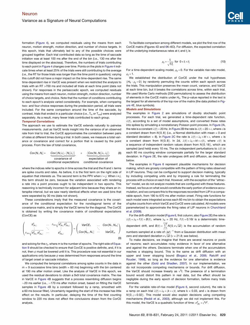
To facilitate comparison among different models, we plot the first row of the
CorCE matrix (Figures 4D and 6K–6O). For diffusion, the expected correlation
of the underlying instantaneous rates at ti and tj is
rij =tiffiffiffiffiffiffititj
p for 0< ti < tj (10)
For a time-dependent scaling model, rij = 0. For the variable rise-rate model,
rij = 1.
We established the distribution of CorCE under the null hypotheses
fH0 : rij = 0g by randomly permuting the counts within each epoch across
the trials. This manipulation preserves the mean count, variance, and VarCE
at each time bin, but it breaks the correlations across time, within each trial.
We used Monte Carlo methods (200 permutations) to assess the distribution
of elements in the CorCE matrix under H0. The p-value reported in the text is
the largest for all elements of the top row of the matrix (the data plotted in Fig-
ure 4E, blue symbols).
Models and Simulations
The examples in Figure 2 are simulations of doubly stochastic point
processes. For each trial, we generated a time-dependent rate function,
lðtÞ, according to a set of model assumptions, and converted these rates
into spikes by simulating a nonstationary Poisson point process. In Figure 2A,
the rate is a constant lðtÞ= 20Hz. In Figure 2B the rate is lðtÞ= 20+ 3, where 3 is
a constant drawn from Nf0; 8g (i.e., a Normal distribution with mean = 0 and
standard deviation = 8). In Figure 2C the rate is lðtÞ= l0 + kt + 3, where 3 is
a constant drawn from Nf0;8g. In 2d, lðtÞ= l0 + kt + 3ðtÞ, where 3ðtÞ is
a sequence of independent random values drawn from Nf0; 18g, which are
sampled (and held) every 10 ms. The six independent perturbations to lðtÞ ineach 60 ms counting window compensate partially for the larger standard
deviation. In Figure 2E, the rate undergoes drift and diffusion, as described
below.
The examples in Figure 6 represent plausible mechanisms for decision
making, which are grossly compatible with the pattern of firing rates observed
in LIP neurons. They can be configured to support decision making, typically
by including competing units and by imposing a rule for terminating the
process with a choice on each trial. However, with the exception of the ‘‘attrac-
tor’’ model, we do not analyze models that are configured with these features.
Instead, we focus on what would constitute the early portion of evidence accu-
mulation, andwe compare this to the responses recorded from LIP in a compa-
rable epoch, from 190 to 670 ms after motion onset. Firing rate functions for
each model were integrated across each 60 ms bin to obtain the expectations
of spike counts fromwhich VarCE andCorCEwere calculated. All models were
parameterized to approximate the firing rates of LIP neurons in Churchland
et al. (2008).
For the drift-diffusionmodel (Figure 6, first column; also Figure 2E) the rate is
lðtÞ= l0 + fðtÞ+BðtÞ, where l0 = 20 Hz, fðtÞ= 0:16t is a deterministic time-
dependent drift, and BðtÞ= Pt=Dti =1
Nf0; v ffiffiffiffiffiDt
p g is the accumulation of random
numbers sampled at a rate of ðDtÞ�1 from a Gaussian distribution with mean
zero and standard deviation vffiffiffiffiffiDt
p(n = 21.8; see below).
To make decisions, we imagine that there are several neurons or pools
of neurons; each accumulates noisy evidence in favor of one alternative
and against the others. Decisions terminate when one of the accumulators
reaches a stopping bound. This is the same as drift diffusion with an
upper and lower stopping bound (Bogacz et al., 2006; Ratcliff and
Rouder, 1998), so long as the evidence for one alternative is evidence
against the other (Gold and Shadlen, 2007). In our implementation, we
do not incorporate competing mechanisms or bounds. For drift diffusion,
the VarCE should increase linearly as n2t. The presence of a termination
bound would distort this pattern in real data, but the effect should be
negligible during the early epoch of decision formation, before many trials
terminate.
For the variable rate-of-rise model (Figure 6, second column), the rate is
a ramp on each trial lðtÞ= l0 + ðk + 3Þt, where k = 0.03, and 3 is drawn from
Nf0; 2= 0:02g. This model would also explain decisions using competing
mechanisms (Reddi et al., 2003), although we did not implement this. For
this model, the VarCE is a quadratic function of time: s2hNi = 22t2.
Neuron 69, 818–831, February 24, 2011 ª2011 Elsevier Inc. 829
Neuron
Variance as a Signature of Neural Computations
For the time-dependent scaling (Figure 6, third column), momentary
evidence is drawn from a positive valued distribution, but the pieces of
evidence are not summed together. Instead, each random value (of evidence)
is weighted by a function, g(t), that increases gradually over time:
lðtÞ= l0 +gðtÞ3ðtÞ, where 3ðtÞ is a sequence of random values drawn from
a stationary gamma distribution (mean = 20 sp/s and standard deviation
2= 0:47) that is sampled (and held) every 10 ms. These values approximate
the average firing rate of a population of weakly correlated MT neurons to
0% coherent motion in a 10 ms sample (Britten et al., 1996). In an epoch
from ti to ti+1, the expected count is the integrated rate:
hNii=Zti + 1
ti
20gðtÞdt (11)
and the VarCE varies quadratically with the gain: s2hNiifg2ðtÞ22. The multiple
independent random samples in each counting window render this expression
approximate. This model would make decisions via competition with other
mechanisms, as in the previous two models.
The probabilistic population code (PPC, Figure 6, fourth column) was imple-
mented using an algorithm that has been described elsewhere (Beck et al.,
2008). We simulated conditions approximating 0% coherence motion, and
we analyze the response of a putative ‘‘right choice’’ LIP neuron during the
early decision formation, regardless of the ultimate outcome of the trial. As
in bounded integration, independent random samples of evidence from
neurons in an MT layer are summed together at each time step in an LIP layer
(for this paper, samples of evidence were generated independently at each
time step, a change from Beck et al., 2008). The neurons also receive excita-
tion and inhibition from other LIP neurons. Absent these inputs, the LIP firing
rates would represent the sum of independent random numbers and would
thus exhibit VarCE like the DDM.
The recurrent nonlinear dynamical ‘‘attractor’’ model (Figure 6, right column)
is described in (Wong et al., 2007). In the model, LIP neurons receive excit-
atory input from simulated MT neurons, recurrent excitation from other
LIP neurons, and inhibition from interneurons, which themselves receive
excitatory and inhibitory input from LIP neurons. The LIP neurons undergo
dynamic changes resembling integration of evidence, followed by divergence
into a stable attractor state in which only a subpopulation of neurons is
active. Parameter values are the same as in (Wong et al., 2007) except
for the following changes. (1) No target inputs were used (for simplicity). (2)
The mean inputs representing random dots stimulus are smaller. Imotion =
JA;extm0ð1± fc0=100Þ, where c0 is the motion coherence, m0 = 30 sp/s,
JA;ext = 1:83310�4 nA/ sp/s, f = 7:2. The ± sign refers to the neural population
for which the motion stimulus is the preferred or null direction, respectively. (3)
The noise standard deviation is increased to 0.075 nA when the stimulus
comes on. More details are available at http://wanglab.med.yale.edu/
webpages/codes.shtml.
We analyzed only the early portion of the activity, corresponding to the
period of evidence accumulation in the physiology. We checked that
the psychometric function and chronometric function of the model are
comparable to the monkey’s behavior (cf. Furman and Wang, 2008) but
did not attempt to quantitatively fit the model to the behavioral data.
Choice and RT on single trials were determined when one of the two neural
pools crossed a firing rate threshold of 40 sp/s. Analysis at each time point
was restricted to trials where both population firing rates were still below
40 sp/s.
For the mixtures (change-point) analysis (Figure 7), we analyzed data from
0% coherence trials ending with a Tin choice, using all neurons. The method
for producing mixtures of responses is described in the main text. Under the
mixture model, the samples comprising the first time bin (centered 190 ms
after motion onset) represent the low state. The Monte Carlo methods repro-
duce the mean as random samples (with replacement) from the same set of
trials and therefore replicate the observedmean and VarCE. For all subsequent
time bins, however, the rate is matched (on average) by sampling appropriate
mixtures from this set of low state rates and the set of responses in a 60ms bin
centered 80 ms before saccade initiation (Tin choices). The VarCE for all 600
samples was larger than the observed VarCE in all but the first time bin, where
they should be identical.
830 Neuron 69, 818–831, February 24, 2011 ª2011 Elsevier Inc.
SUPPLEMENTAL INFORMATION
Supplemental Information includes five figures and can be found with this
article online at doi:10.1016/j.neuron.2010.12.037.
ACKNOWLEDGMENTS
We thank Greg Horwitz, Eric Shea-Brown, Mehrdad Jazayeri, and Mark
Churchland for helpful advice. This work was supported by NIH EY011378,
EY019072, RR00166, MH062349 (X.J.W.), DA022780 (A.P.), the McDonnell
Foundation (A.P.), the Kavli Foundation (X.J.W.), andHHMI (M.N.S.). Additional
support is as follows: NIH EY019072 (A.K.C.), NIH MH062349 and the Kavli
Foundation (X.-J.W.), MURI grant N00014-07-1-0937 (A.P.), NIDA grant
#BCS0346785 (A.P., M.N.), research grant from the James S. McDonnell
Foundation (A.P., M.N.S.), P30 EY001319 (partial support; A.P.), HHMI
(M.S.), NIDA #BCS0346785 (A.P., M.S.), NIH EY011378, research grant from
the James S. McDonnell Foundation (A.P., M.S.), and NIH RR00166 (M.S.).
Accepted: December 3, 2010
Published: February 23, 2011
REFERENCES
Aertsen, A.M., Gerstein, G.L., Habib, M.K., and Palm, G. (1989). Dynamics
of neuronal firing correlation: Modulation of ‘‘effective connectivity’’.
J. Neurophysiol. 61, 900–917.
Albantakis, L., and Deco, G. (2009). The encoding of alternatives in multiple-
choice decision making. Proc. Natl. Acad. Sci. USA 106, 10308–10313.
Balan, P.F., Oristaglio, J., Schneider, D.M., and Gottlieb, J. (2008). Neuronal
correlates of the set-size effect in monkey lateral intraparietal area. PLoS
Biol. 6, e158.
Barlow, H.B. (1956). Retinal noise and absolute threshold. J. Opt. Soc. Am. 46,
634–639.
Basso, M.A., and Wurtz, R.H. (1998). Modulation of neuronal activity in supe-
rior colliculus by changes in target probability. J. Neurosci. 18, 7519–7534.
Beck, J.M., Ma, W.J., Kiani, R., Hanks, T., Churchland, A.K., Roitman, J.,
Shadlen, M.N., Latham, P.E., and Pouget, A. (2008). Probabilistic population
codes for Bayesian decision making. Neuron 60, 1142–1152.
Berry, M.J., 2nd, and Meister, M. (1998). Refractoriness and neural precision.
J. Neurosci. 18, 2200–2211.
Bogacz, R., Brown, E., Moehlis, J., Holmes, P., and Cohen, J.D. (2006). The
physics of optimal decision making: A formal analysis of models of perfor-
mance in two-alternative forced-choice tasks. Psychol. Rev. 113, 700–765.
Britten, K.H., Newsome, W.T., Shadlen, M.N., Celebrini, S., andMovshon, J.A.
(1996). A relationship between behavioral choice and the visual responses of
neurons in macaque MT. Vis. Neurosci. 13, 87–100.
Britten, K.H., Shadlen, M.N., Newsome, W.T., and Movshon, J.A. (1992). The
analysis of visual motion: A comparison of neuronal and psychophysical
performance. J. Neurosci. 12, 4745–4765.
Britten, K.H., Shadlen, M.N., Newsome, W.T., and Movshon, J.A. (1993).
Responses of neurons in macaque MT to stochastic motion signals. Vis.
Neurosci. 10, 1157–1169.
Bulmer, M.G., Howarth, C.I., Cane, V., Gregory, R.L., and Barlow, H.B. (1957).
Noise and the visual threshold. Nature 180, 1403–1405.
Carpenter, R.H., and Williams, M.L. (1995). Neural computation of log likeli-
hood in control of saccadic eye movements. Nature 377, 59–62.
Churchland, A.K., Kiani, R., and Shadlen, M.N. (2008). Decision-making with
multiple alternatives. Nat. Neurosci. 11, 693–702.
Churchland, M.M., Yu, B.M., Cunningham, J.P., Sugrue, L.P., Cohen, M.R.,
Corrado, G.S., Newsome, W.T., Clark, A.M., Hosseini, P., Scott, B.B., et al.
(2010). Stimulus onset quenches neural variability: A widespread cortical
phenomenon. Nat. Neurosci. 13, 369–378.
Neuron
Variance as a Signature of Neural Computations
Churchland, M.M., Yu, B.M., Ryu, S.I., Santhanam, G., and Shenoy, K.V.
(2006). Neural variability in premotor cortex provides a signature of motor
preparation. J. Neurosci. 26, 3697–3712.
Cisek, P., Puskas, G.A., and El-Murr, S. (2009). Decisions in changing condi-
tions: The urgency-gating model. J. Neurosci. 29, 11560–11571.
Cox, D.R., and Isham, V. (1980). Point Processes (London, New York:
Chapman and Hall).
Daley, D.J., and Vere-Jones, D. (2003). Elementary theory and methods. In An
Introduction to the Theory of Point Processes (New York: Springer).
Faisal, A.A., Selen, L.P., and Wolpert, D.M. (2008). Noise in the nervous
system. Nat. Rev. Neurosci. 9, 292–303.
Furman, M., and Wang, X.J. (2008). Similarity effect and optimal control of
multiple-choice decision making. Neuron 60, 1153–1168.
Geisler, W.S., and Albrecht, D.G. (1995). Bayesian analysis of identification
performance in monkey visual cortex: Nonlinear mechanisms and stimulus
certainty. Vision Res. 35, 2723–2730.
Geisler, W.S., Albrecht, D.G., Crane, A.M., and Stern, L. (2001). Motion direc-
tion signals in the primary visual cortex of cat and monkey. Vis. Neurosci. 18,
501–516.
Glimcher, P.W. (2005). Indeterminacy in brain and behavior. Annu. Rev.
Psychol. 56, 25–56.
Gold, J.I., and Shadlen, M.N. (2007). The neural basis of decision making.
Annu. Rev. Neurosci. 30, 535–574.
Gottlieb, J., and Balan, P. (2010). Attention as a decision in information space.
Trends Cogn. Sci. 14, 240–248.
Hanes, D.P., and Schall, J.D. (1996). Neural control of voluntary movement
initiation. Science 274, 427–430.
Huk, A.C., and Shadlen, M.N. (2005). Neural activity inmacaque parietal cortex
reflects temporal integration of visual motion signals during perceptual deci-
sion making. J. Neurosci. 25, 10420–10436.
Keat, J., Reinagel, P., Reid, R.C., and Meister, M. (2001). Predicting every
spike: A model for the responses of visual neurons. Neuron 30, 803–817.
Lewis, J.W., and Van Essen, D.C. (2000). Mapping of architectonic subdivi-
sions in the macaque monkey, with emphasis on parieto-occipital cortex.
J. Comp. Neurol. 428, 79–111.
Machens, C.K., Romo, R., and Brody, C.D. (2005). Flexible control of mutual
inhibition: A neural model of two-interval discrimination. Science 307, 1121–
1124.
Maimon, G., and Assad, J.A. (2009). Beyond Poisson: Increased spike-time
regularity across primate parietal cortex. Neuron 62, 426–440.
McAdams, C.J., andMaunsell, J.H. (1999). Effects of attention on the reliability
of individual neurons in monkey visual cortex. Neuron 23, 765–773.
Miller, P., andWang, X.J. (2006). Power-law neuronal fluctuations in a recurrent
network model of parametric working memory. J. Neurophysiol. 95, 1099–
1114.
Nawrot, M.P., Boucsein, C., Rodriguez Molina, V., Riehle, A., Aertsen, A., and
Rotter, S. (2008). Measurement of variability dynamics in cortical spike trains.
J. Neurosci. Methods 169, 374–390.
Parker, A.J., and Newsome,W.T. (1998). Sense and the single neuron: Probing
the physiology of perception. Annu. Rev. Neurosci. 21, 227–277.
Ratcliff, R., and Rouder, J.N. (1998). Modeling response times for two-choice
decisions. Psychol. Sci. 9, 347–356.
Reddi, B.A., Asrress, K.N., and Carpenter, R.H. (2003). Accuracy, information,
and response time in a saccadic decision task. J. Neurophysiol. 90, 3538–
3546.
Romo, R., and Salinas, E. (2001). Touch and go: Decision-making mechanisms
in somatosensation. Annu. Rev. Neurosci. 24, 107–137.
Shadlen, M.N., and Newsome, W.T. (1998). The variable discharge of cortical
neurons: Implications for connectivity, computation, and information coding.
J. Neurosci. 18, 3870–3896.
Smith, P.L., and Ratcliff, R. (2004). Psychology and neurobiology of simple
decisions. Trends Neurosci. 27, 161–168.
Softky, W.R., and Koch, C. (1993). The highly irregular firing of cortical cells is
inconsistent with temporal integration of random EPSPs. J. Neurosci. 13,
334–350.
Teich, M.C., Heneghan, C., Lowen, S.B., Ozaki, T., and Kaplan, E. (1997).
Fractal character of the neural spike train in the visual system of the cat.
J. Opt. Soc. Am. A Opt. Image Sci. Vis. 14, 529–546.
Tolhurst, D.J., and Heeger, D.J. (1997). Comparison of contrast-normalization
and threshold models of the responses of simple cells in cat striate cortex. Vis.
Neurosci. 14, 293–309.
Tolhurst, D.J., Movshon, J.A., and Dean, A.F. (1983). The statistical reliability
of signals in single neurons in cat and monkey visual cortex. Vision Res. 23,
775–785.
Usher, M., and McClelland, J.L. (2001). The time course of perceptual choice:
The leaky, competing accumulator model. Psychol. Rev. 108, 550–592.
Vaadia, E., Haalman, I., Abeles, M., Bergman, H., Prut, Y., Slovin, H., and
Aertsen, A. (1995). Dynamics of neuronal interactions in monkey cortex in
relation to behavioural events. Nature 373, 515–518.
Wang, X.J. (2002). Probabilistic decision making by slow reverberation in
cortical circuits. Neuron 36, 955–968.
Wong, K.F., Huk, A.C., Shadlen, M.N., and Wang, X.J. (2007). Neural circuit
dynamics underlying accumulation of time-varying evidence during perceptual
decision making. Front. Comput. Neurosci. 1, 6.
Neuron 69, 818–831, February 24, 2011 ª2011 Elsevier Inc. 831
Recommended