Variational assimilation: method & technicalities
Claude Fischer & Patrick Moll,CNRM/GMAP, Météo-France
Overview of some principles of VAR assimilation as applied in our NWP systems
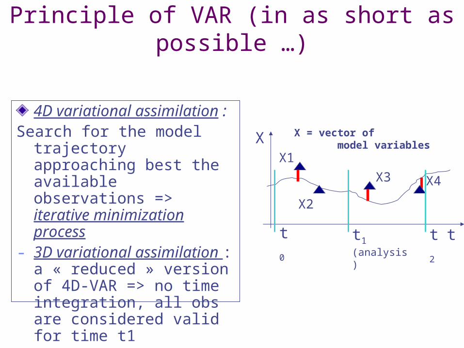
Principle of VAR (in as short as possible …)
t
XX1
X2
X3 X4
t1
(analysis)
X = vector of model variables
t2
t0
4D variational assimilation :
Search for the model trajectory approaching best the available observations => iterative minimization process
- 3D variational assimilation : a « reduced » version of 4D-VAR => no time integration, all obs are considered valid for time t1
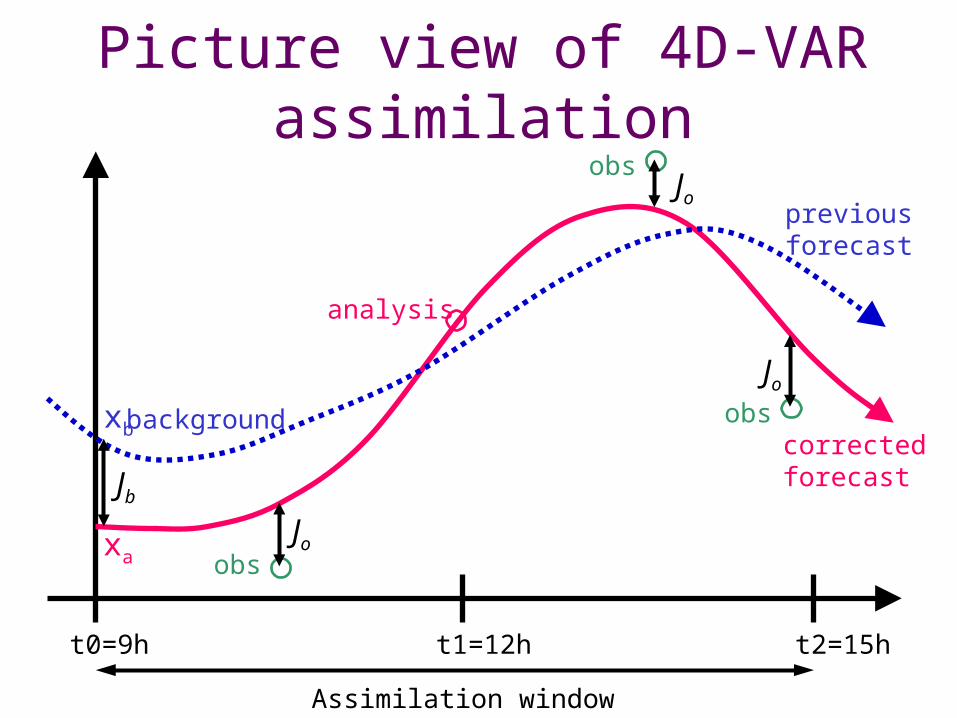
Picture view of 4D-VAR assimilation
t0=9h t1=12h t2=15h
Assimilation window
Jb
Jo
Jo
Jo
obs
obs
obs
analysis
xa
xbcorrectedforecast
previousforecast
background
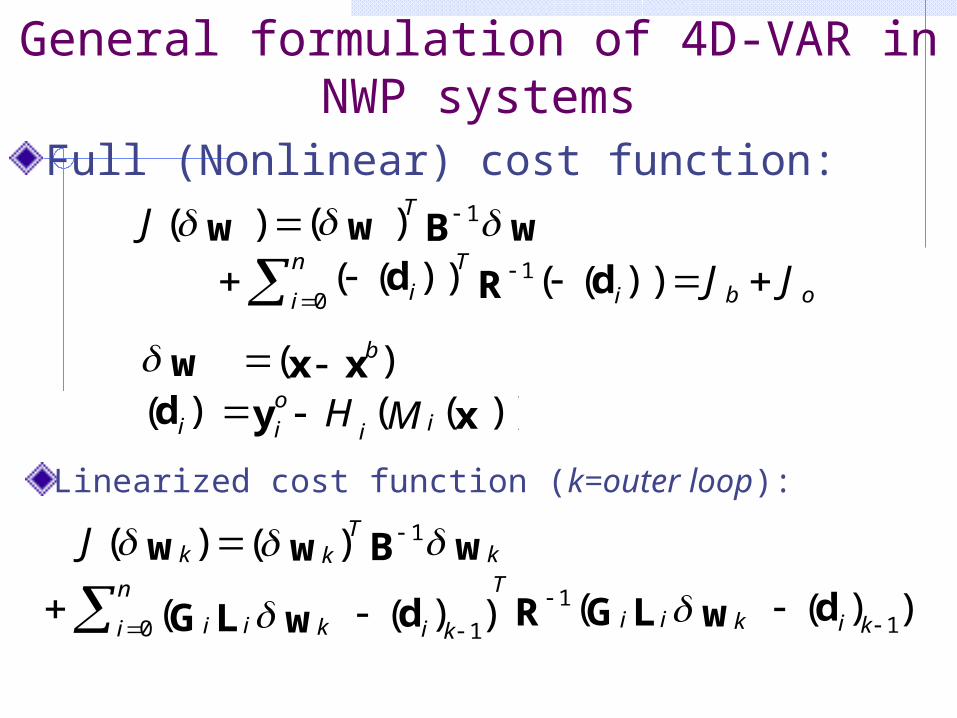
General formulation of 4D-VAR in NWP systems
Full (Nonlinear) cost function:
wBww 1)()( TJ
ob
n
i ii
TJJ
0
1 ))(())(( dRd
wBww kkT
kJ 1)()(
n
i i kkiii kkii
T
0 11
1))(())(( dwLGRdwLG
)( xxw b))(()( xyd MH i
oi ii
Linearized cost function (k=outer loop):
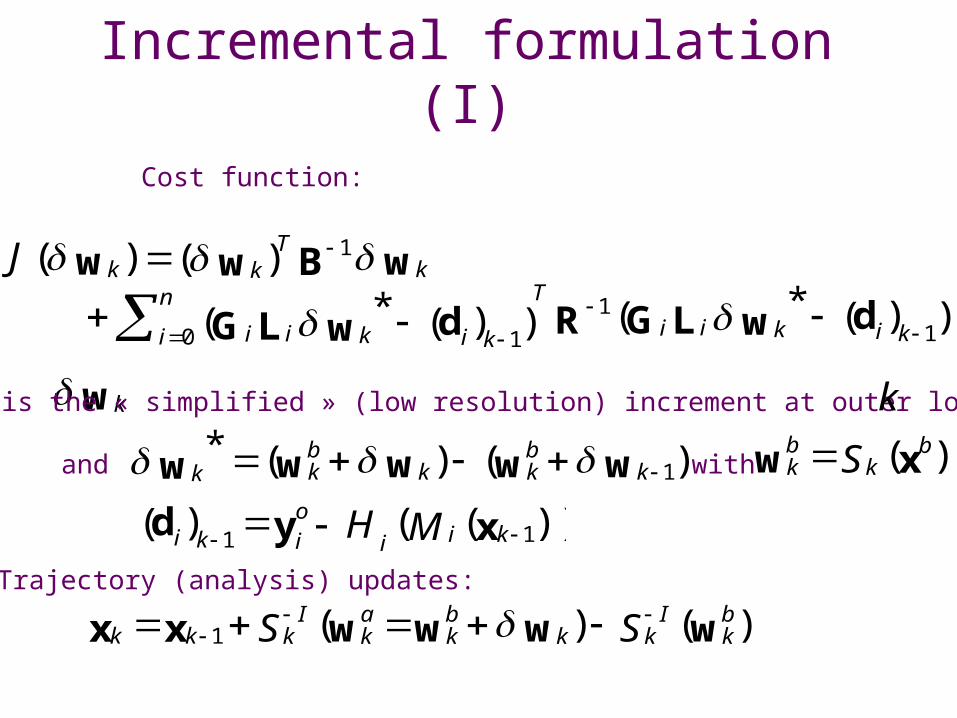
Incremental formulation (I)Cost function:
wBww kkT
kJ 1)()(
n
i i kkiii kkii
T
0 11
1))(*())(*( dwLGRdwLG
wk is the « simplified » (low resolution) increment at outer loop k
)()(*1wwwww k
bkk
bkk
))(()( 11 xyd kioi ii k MH
and
Trajectory (analysis) updates:
)()(1 wwwwxx bk
Ikk
bk
ak
Ikkk SS
with )(xw bk
bk S
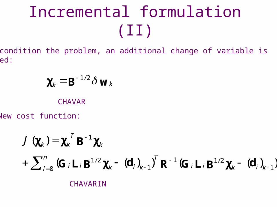
Incremental formulation (II)To pre-condition the problem, an additional change of variable is performed:
χBχχ kk
T
kJ 1)(
n
i i kkiii kkiiT
0 12/11
12/1 ))(())(( dχBLGRdχBLG
wBχ kk 2/1
CHAVAR
New cost function:
CHAVARIN

Incremental 4D-Var algorithm
(ECMWF documentation)
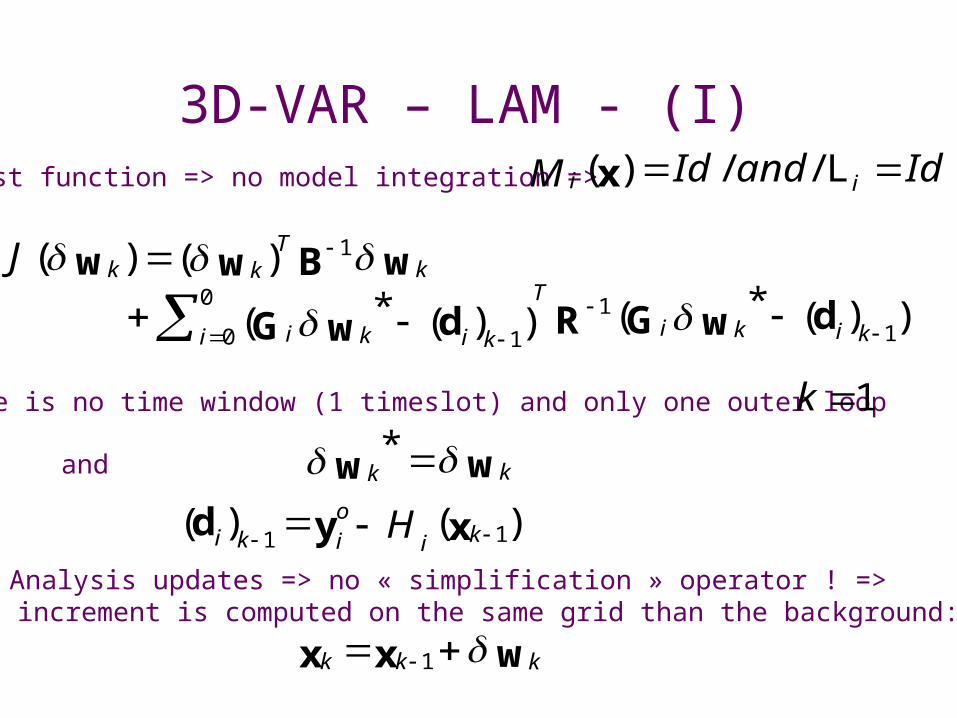
3D-VAR – LAM - (I)Cost function => no model integration =>
wBww kkT
kJ 1)()(
0
0 11
1))(*())(*(i i kkii kki
TdwGRdwG
There is no time window (1 timeslot) and only one outer loop 1k
ww kk *
)()( 11 xyd koi ii k H
and
Analysis updates => no « simplification » operator ! => the increment is computed on the same grid than the background:
wxx kkk 1
IdandIdM ii L//)(x
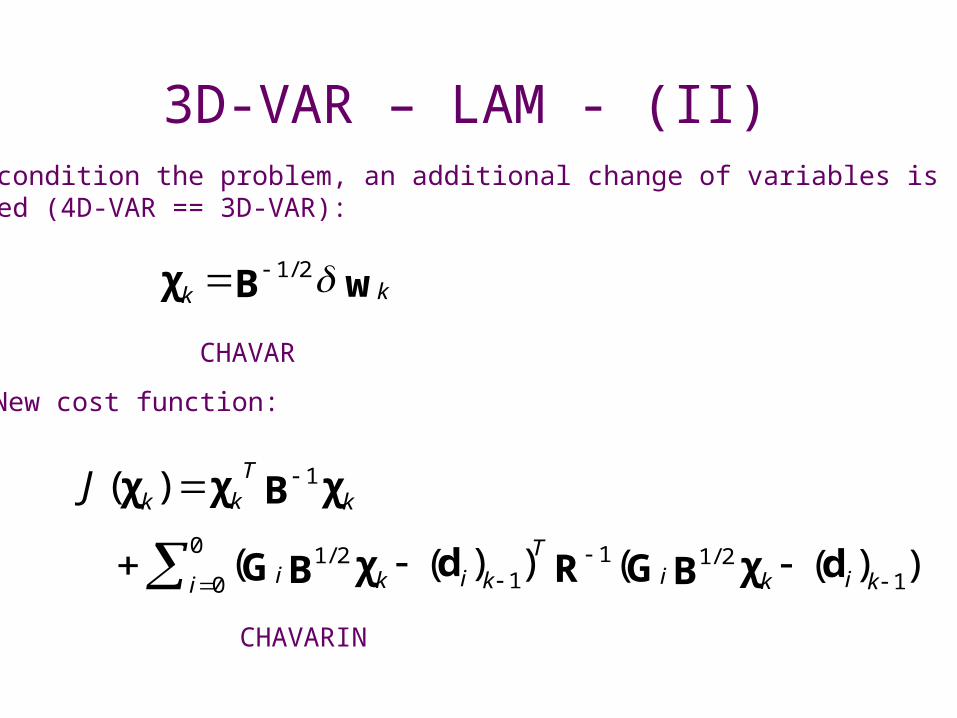
3D-VAR – LAM - (II)To pre-condition the problem, an additional change of variables is Performed (4D-VAR == 3D-VAR):
χBχχ kk
T
kJ 1)(
0
0 12/11
12/1 ))(())((
i i kkii kkiT
dχBGRdχBG
wBχ kk 2/1
CHAVAR
New cost function:
CHAVARIN
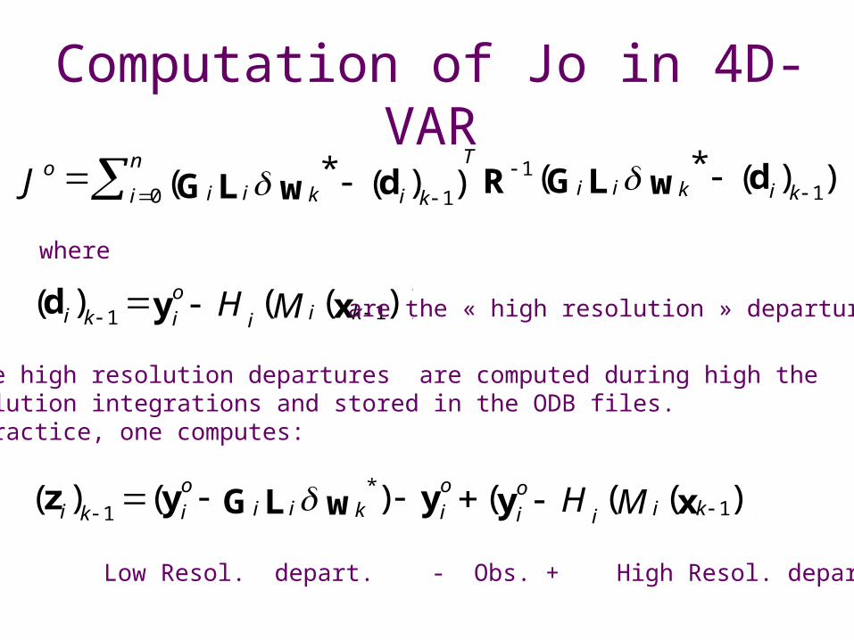
Computation of Jo in 4D-VAR
n
i i kkiii kkii
ToJ 0 1
1
1))(*())(*( dwLGRdwLG
))(()( 11 xyd kioi ii k MH
These high resolution departures are computed during high the resolution integrations and stored in the ODB files.In practice, one computes:
where
are the « high resolution » departures.
))((()()( 1*
1 xyywLGyz kioi i
oikii
oii k MH
Low Resol. depart. - Obs. + High Resol. depart.
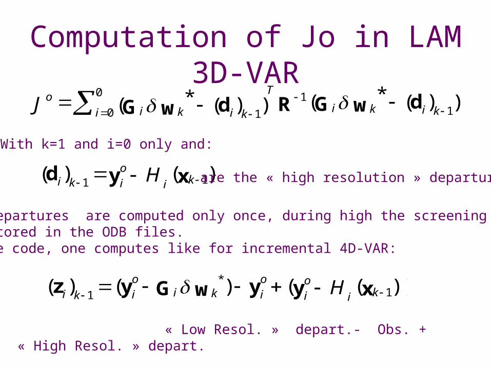
Computation of Jo in LAM 3D-VAR
0
0 11
1))(*())(*(i i kkii kki
ToJ dwGRdwG
)()( 11 xyd koi ii k H
The departures are computed only once, during high the screening step and stored in the ODB files. In the code, one computes like for incremental 4D-VAR:
With k=1 and i=0 only and:
are the « high resolution » departures.
))(()()( 1*
1 xyywGyz koi i
oiki
oii k H
« Low Resol. » depart.- Obs. + « High Resol. » depart.
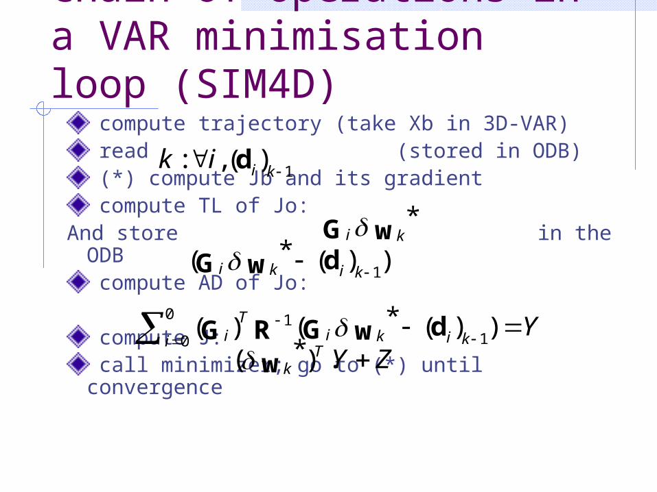
Chain of operations in a VAR minimisation loop (SIM4D)
compute trajectory (take Xb in 3D-VAR) read (stored in ODB) (*) compute Jb and its gradient compute TL of Jo:
And store in the ODB compute AD of Jo:
compute J: call minimizer; go to (*) until convergence
wG ki *
Yi i kkii
T 0
0 11 ))(*()( dwGRG
))(*(1dwG i kki
ZYTk .)*( w
)(,:1di k
ik
Major messages to keep in mind:
3D-VAR is a reduced (« simpler ») version of 4D-VAR Aladin 3D-VAR is a code installed inside the global IFS/Arpège code (as we will see in the last slides)
Back to application … with pictures !
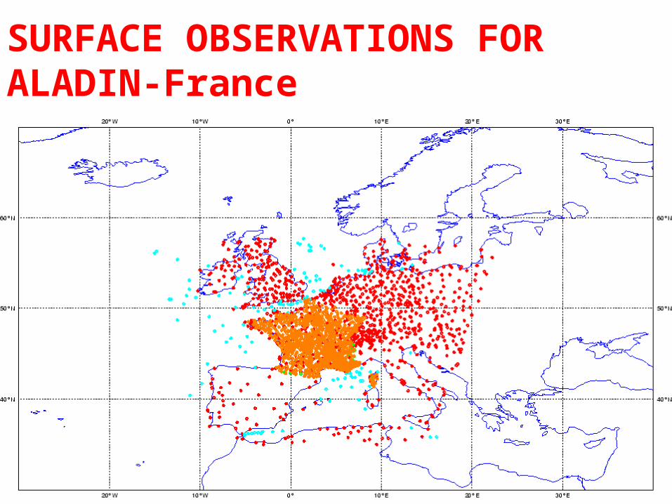
SURFACE OBSERVATIONS FOR ALADIN-France
Resolution volum, ray path : standard refraction (4/3 Earth’radius)
zh
rd
eZ
r
Nd
d
model level
• Bi-linear interpolation of the simulated hydrometeors (T,q, qr, qs, qg) • Compute « radar reflectivity » on each model level
Backscattering cross section: Rayleigh (attenuation neglected)
..., 0
),().,()(snowrainj
dDrDNjrDjr
Microphysic Scheme in AROME
Diameter of particules
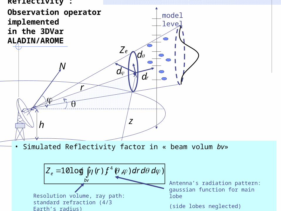
• Simulated Reflectivity factor in « beam volum bv»
Antenna’s radiation pattern: gaussian function for main lobe
(side lobes neglected)
)..).,().(log10 4 dddrfr(Zbv
e
Resolution volume, ray path: standard refraction (4/3 Earth’s radius)
Assimilation of Reflectivity : Observation operator implemented in the 3DVar ALADIN/AROME
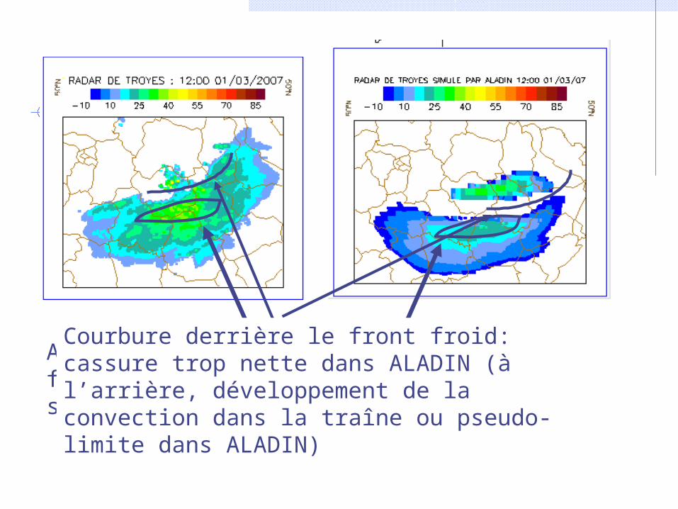
Apparition de bande étroite de front froid: moins intense et légèrement plus sud dans ALADIN.
Courbure derrière le front froid: cassure trop nette dans ALADIN (à l’arrière, développement de la convection dans la traîne ou pseudo-limite dans ALADIN)
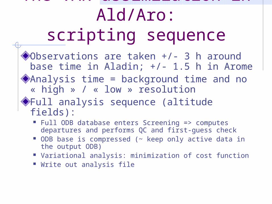
The VAR assimilation in Ald/Aro:
scripting sequenceObservations are taken +/- 3 h around base time in Aladin; +/- 1.5 h in AromeAnalysis time = background time and no « high » / « low » resolutionFull analysis sequence (altitude fields):
Full ODB database enters Screening => computes departures and performs QC and first-guess check
ODB base is compressed (~ keep only active data in the output ODB)
Variational analysis: minimization of cost function Write out analysis file
Technical aspects about the LAM VAR code inside the IFS
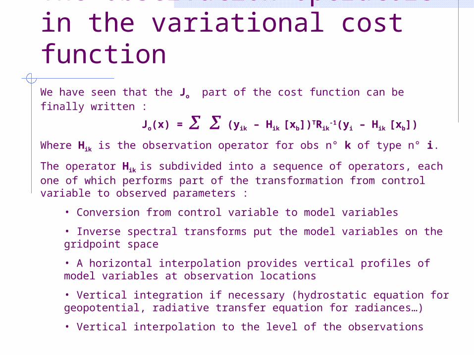
The observation operators in the variational cost functionWe have seen that the Jo part of the cost function can be finally written :
Jo(x) = (yik – Hik [xb])TRik-1(yi – Hik [xb])
Where Hik is the observation operator for obs n° k of type n° i.
The operator Hik is subdivided into a sequence of operators, each one of which performs part of the transformation from control variable to observed parameters :
• Conversion from control variable to model variables
• Inverse spectral transforms put the model variables on the gridpoint space
• A horizontal interpolation provides vertical profiles of model variables at observation locations
• Vertical integration if necessary (hydrostatic equation for geopotential, radiative transfer equation for radiances…)
• Vertical interpolation to the level of the observations
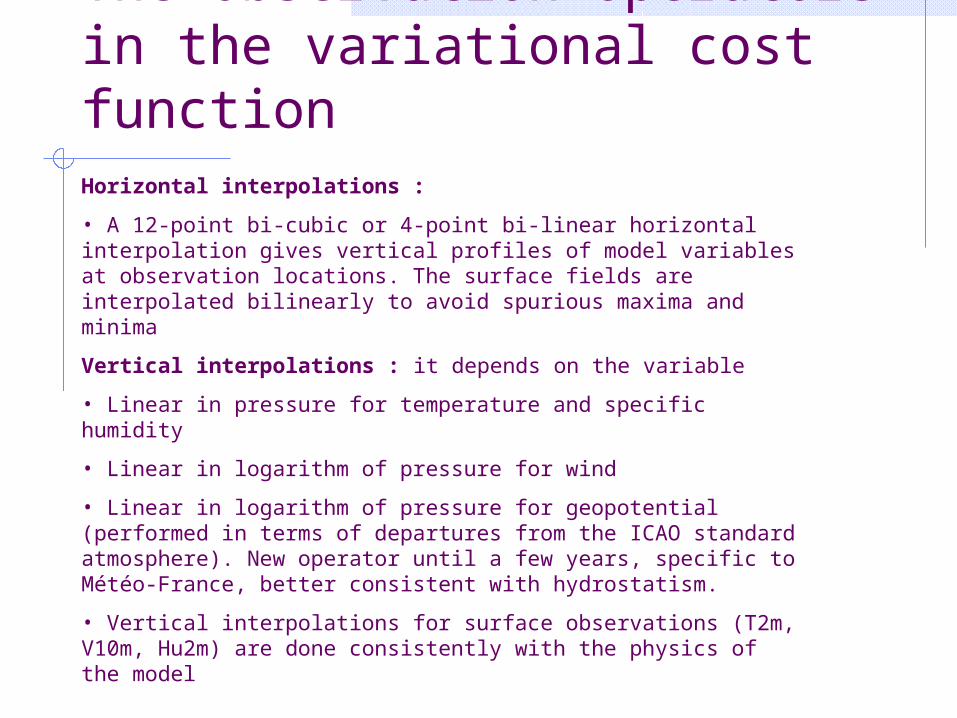
The observation operators in the variational cost functionHorizontal interpolations :
• A 12-point bi-cubic or 4-point bi-linear horizontal interpolation gives vertical profiles of model variables at observation locations. The surface fields are interpolated bilinearly to avoid spurious maxima and minima
Vertical interpolations : it depends on the variable
• Linear in pressure for temperature and specific humidity
• Linear in logarithm of pressure for wind
• Linear in logarithm of pressure for geopotential (performed in terms of departures from the ICAO standard atmosphere). New operator until a few years, specific to Météo-France, better consistent with hydrostatism.
• Vertical interpolations for surface observations (T2m, V10m, Hu2m) are done consistently with the physics of the model
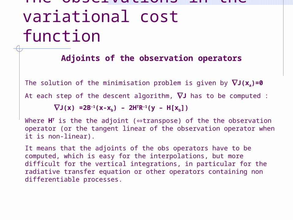
Adjoints of the observation operators
The solution of the minimisation problem is given by J(xa)=0
At each step of the descent algorithm, J has to be computed :
J(x) =2B-1(x-xb) – 2HTR-1(y – H[xb])
Where HT is the the adjoint (transpose) of the the observation operator (or the tangent linear of the observation operator when it is non-linear).
It means that the adjoints of the obs operators have to be computed, which is easy for the interpolations, but more difficult for the vertical integrations, in particular for the radiative transfer equation or other operators containing non differentiable processes.
The observations in the variational cost function
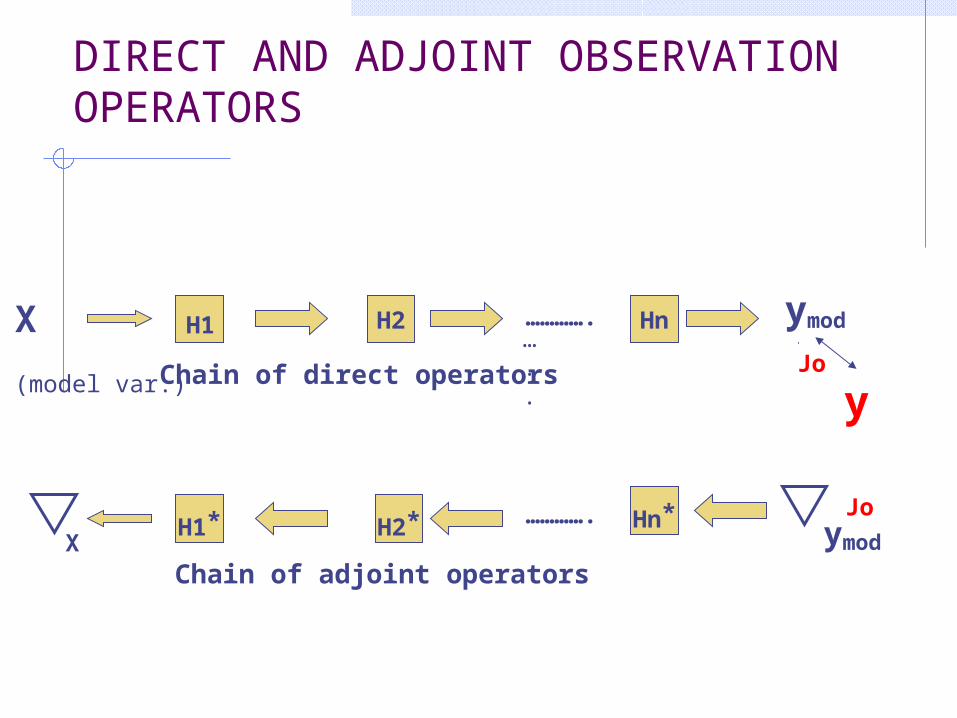
DIRECT AND ADJOINT OBSERVATION OPERATORS
H1 HnH2
H1* H2* Hn*
…..
………….
………….
X
(model var.)
ymod
X ymod
yJo
Jo
Chain of direct operators
Chain of adjoint operators

Chain of operations in a VAR minimisation loop (SIM4D)
compute trajectory (take Xb in 3D-VAR) read (stored in ODB) (*) compute Jb and its gradient compute TL of Jo:
And store in the ODB compute AD of Jo:
compute J: call minimizer; go to (*) until convergence
wG ki *
Yi i kkii
T 0
0 11 ))(*()( dwGRG
))(*(1dwG i kki
ZYTk .)*( w
)(,:1di k
ik
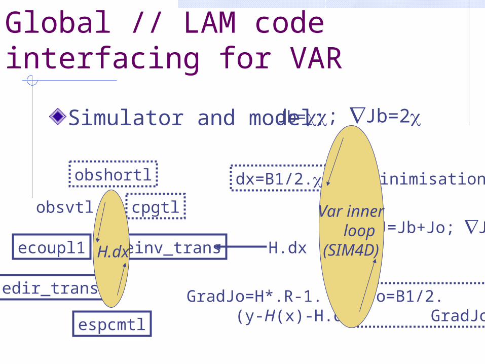
Global // LAM code interfacing for VAR
Simulator and model:
H.dx
Jo=B1/2. GradJo
J=Jb+Jo; J
Minimisation
Jb=; Jb=2
GradJo=H*.R-1. (y-H(x)-H.dx)
dx=B1/2.
einv_trans
cpgtl
obshortl
obsvtl
edir_trans
ecoupl1
espcmtl
H.dx
Var inner loop
(SIM4D)
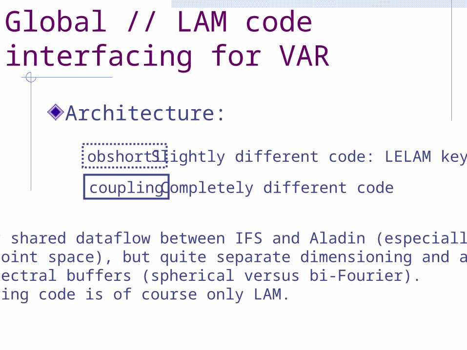
Global // LAM code interfacing for VAR
Architecture:
obshortl
coupling
Slightly different code: LELAM key
Completely different code
Fully shared dataflow between IFS and Aladin (especially ingridpoint space), but quite separate dimensioning and addressingin spectral buffers (spherical versus bi-Fourier).Coupling code is of course only LAM.
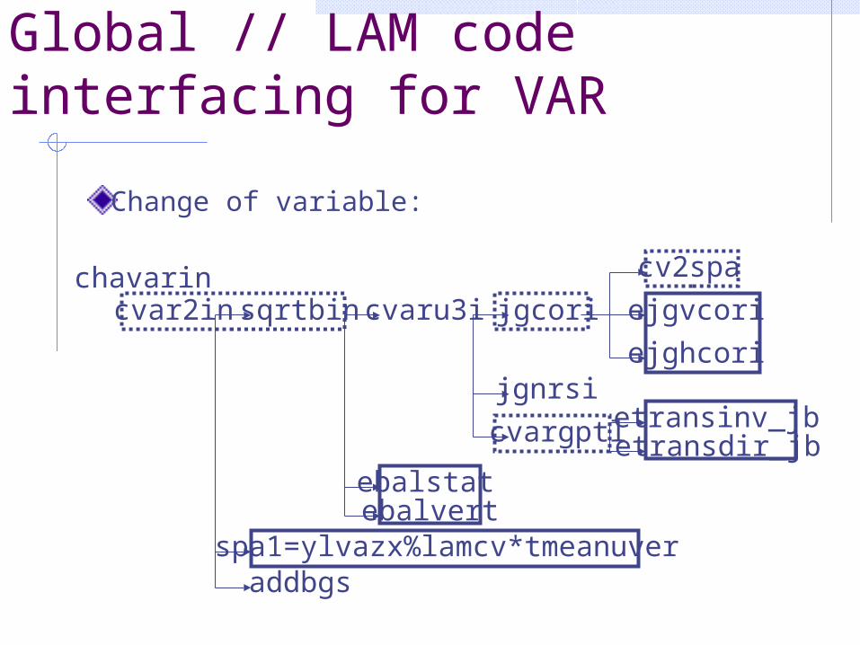
Global // LAM code interfacing for VAR
Change of variable:
chavarincvar2in sqrtbin cvaru3i jgcori
cv2spa
ejgvcori
jgnrsi
cvargptl etransinv_jbetransdir_jb
ebalstatebalvert
spa1=ylvazx%lamcv*tmeanuveraddbgs
ejghcori
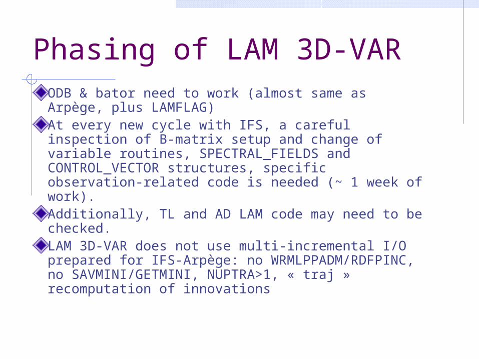
Phasing of LAM 3D-VARODB & bator need to work (almost same as Arpège, plus LAMFLAG)At every new cycle with IFS, a careful inspection of B-matrix setup and change of variable routines, SPECTRAL_FIELDS and CONTROL_VECTOR structures, specific observation-related code is needed (~ 1 week of work). Additionally, TL and AD LAM code may need to be checked.LAM 3D-VAR does not use multi-incremental I/O prepared for IFS-Arpège: no WRMLPPADM/RDFPINC, no SAVMINI/GETMINI, NUPTRA>1, « traj » recomputation of innovations
Thank you for your attention
Recommended