Vehicle Axle Detection and Spacing Calibration Using
MEMS Accelerometer
Wei Zhang
Thesis submitted to the faculty of the Virginia Polytechnic Institute and State University
in partial fulfillment of the requirements for the degree of
Master of Science
In
Civil and Environmental Engineering
Linbing Wang
Montasir M. Abbas
Cristian Druta
09/18/2014
Blacksburg, VA
Keywords: Vehicle Classification, MEMS Accelerometer, MMLS3, Dynamic Analysis
Vehicle Axle Detection and Spacing Calibration Using
MEMS Accelerometer
Wei Zhang
ABSTRACT
Vehicle classification data especially trucks has an important role in both pavement
maintenance and highway planning strategy. An advanced microelectromechanical
system (MEMS) accelerometer for vehicle classification based on axle count and spacing
was designed, tested, and applied to the pavement. Vehicle-pavement interaction was
collected by the vibration sensor while vehicle axle count and spacing were calibrated
later. Collected vibration data also used to analyze the pavement surface condition and
compared with simulation using dynamic loading analysis. Laboratory tests using
MMLS3 device to verify the accuracy of MEMS accelerometer and reaction under
different surface condition were tested. An algorithm for calculating axle spacing and
axle count was developed. Acceleration of different pavement surface condition were
analyzed and compared with simulation results, the influence of surface condition to the
pavement acceleration was concluded.

iii
Acknowledgements
Foremost, I would like to express my sincere gratitude to my advisor Prof. Linbing Wang
for the continuous support of my Master study and research, for his patience, motivation,
enthusiasm, and immense knowledge. His guidance helped me in all the time of research
and writing of this thesis. I also acknowledge the advisory committee including Dr.
Montasir Abbas and Dr. Cristian Druta for all of their time and assistance during this
project. I also acknowledges the contributions of the structure’s laboratory staff for all of
their assistance during the research process, especially those made by David. A special
acknowledgement goes to Haocheng Xiong and Wenjing Xue for all of their help in the
laboratory and in the field. Finally, the author would like to thank parents Yunan Zhang
and Yuelan Zha for all of their support, encouragement, and love throughout all
academic endeavors. Thanks everyone for your support.
iv
Table of Contents 1. Introduction ......................................................................................................... 1
Background ......................................................................................................... 1 Objectives ........................................................................................................... 2
Outline of the Thesis ........................................................................................... 2 2. Literature Review................................................................................................ 4
Instruction ........................................................................................................... 4 Reviews ............................................................................................................... 5
Traffic Monitoring Theory .......................................................................... 5
Vehicle Classification ................................................................................. 7 Detection Methods ...................................................................................... 7 MEMS Accelerometer .............................................................................. 12
Dynamic Loading Analysis....................................................................... 15 Summary of Findings ........................................................................................ 18
3. Laboratory Tests Using MMLS3 ...................................................................... 20
MEMS Accelerometer Selection ...................................................................... 20 Experiment Setup .............................................................................................. 20
Test Procedures ................................................................................................. 24 Pavement Acceleration Tests .................................................................... 24 MMLS3 Speed Tests................................................................................. 26
4. Dynamic Loading Simulation ........................................................................... 27 Necessity of Using Dynamic Analysis ............................................................. 27
Finite Element Model Geometry .............................................................. 27 Boundary Condition .................................................................................. 29 Loading System ........................................................................................ 29
5. Experimental and Simulation Results Analysis ................................................ 31
Axle Detection Algorithm................................................................................. 31 Axle Spacing and Speed Estimation ................................................................. 35 Experimental Results and Verification ............................................................. 35
Sensor Performance .................................................................................. 36 Axle Count ................................................................................................ 38
Axle Spacing and Speed Verification ....................................................... 39 Sensor Performance with a Crack on Slab ................................................ 41
Simulation Results Analysis ............................................................................. 46 Simulation Results without Crack ............................................................ 47 Simulation Results with a Crack ............................................................... 49
6. Deployment on Plantation Road ....................................................................... 52
Installation Procedures ...................................................................................... 52 Test Results and Analysis ................................................................................. 53
7. Conclusions and Future Work .......................................................................... 57
Vehicle Classification Based on MEMS Accelerometer .................................. 57 Pavement Condition Analysis Based on Acceleration...................................... 58
References ................................................................................................................. 60
v
List of Tables
Table 1 Comparison between Different Methods ............................................................... 8
Table 2 Correction Speed.................................................................................................. 26 Table 3 Noise RMS and Signal Amplitude....................................................................... 36 Table 4 Sensor Axle Count Performance(X-Axle) ........................................................... 38 Table 5 Sensor Axle Count Performance(Y-Axle) ........................................................... 38 Table 6 Sensor Axle Count Performance (Z-Axle) .......................................................... 38
Table 7 Axle Spacing Summary ....................................................................................... 40 Table 8 Speed Verification Summary ............................................................................... 41 Table 9 Standard Deviation Comparison .......................................................................... 43 Table 10 Standard Devotion Comparison from Simulation ............................................. 51
vi
List of Figures Figure 1 Accelerometer Structure ..................................................................................... 14 Figure 2 Sensor Fixed to the Plate .................................................................................... 21
Figure 3 Broad View of the Plate ..................................................................................... 22 Figure 4 Slab with a Crack ................................................................................................ 23 Figure 5 Broad View of MMLS3...................................................................................... 24 Figure 6 Interface of the Software .................................................................................... 25 Figure 7 Flow Chart of Test Procedures ........................................................................... 26
Figure 8 3-D Model of Slab without Crack ...................................................................... 28 Figure 9 3-D Model of Slab with Crack ........................................................................... 29 Figure 10 Data Analysis Process ...................................................................................... 33 Figure 11 Original Output Signal ..................................................................................... 33
Figure 12 Optimized Signal .............................................................................................. 34 Figure 13 Signal after Passing Moving Average Filter .................................................... 34 Figure 14 OM-CP-ULTRASHOCK-5 Shock Recorder Channel 4 Shock - X Axis (g) .. 36
Figure 15 OM-CP-ULTRASHOCK-5 Shock Recorder Channel 5 Shock - Y Axis (g) .. 37 Figure 16 OM-CP-ULTRASHOCK-5 Shock Recorder Channel 6 Shock - Z Axis (g) ... 37
Figure 17 Axle Spacing ................................................................................................... 40 Figure 18 Sensor Performance with No Crack ................................................................. 42 Figure 19 Sensor Performance with a Crack .................................................................... 42
Figure 20 Slab without Crack ........................................................................................... 44 Figure 21 Slab with a Crack.............................................................................................. 45
Figure 22 Vertical Acceleration ........................................................................................ 47 Figure 23 Simulation Results of Acceleration .................................................................. 48 Figure 24 Single Wheel-Passing Comparison between Sensor and Simulation ............... 49
Figure 25 Simulation Results of Acceleration .................................................................. 50
Figure 26 Single Wheel-Passing Comparison between Sensor and Simulation ............... 51 Figure 27 Sensor Installed on Pavement ........................................................................... 52 Figure 28 Sensor Location on Pavement .......................................................................... 53
Figure 29 Z-axis Acceleration from Pavement Test. ........................................................ 54 Figure 30 Static Noise Signal ........................................................................................... 55 Figure 31 Optimized Signal .............................................................................................. 55
1
1. Introduction
Background
Vehicle classification, especially truck and other heavy-loading vehicle, is considered
significantly for transportation engineering and pavement health monitoring. Current
classification technologies including intrusive and non-intrusive technologies. Intrusive
technologies like piezoelectric sensors and inductive loop detectors have very high
maintenance costs and complicit installation processes under pavement which may need
lane closing and possibly cause both pavement and sensor damage in the further. Non-
intrusive technologies like video imaging and ultrasonic sensors are sensitive to weather
condition which may influence the accuracy. In this case, a convenient method which
sensors installed on the shoulder of the pavement without subjecting to vehicle loading
should be considered and tested. An accelerometer is a device that measures acceleration
force which can be used to monitor the vehicle-pavement interaction. There are different
kinds of accelerometers, most common used is piezoelectric crystal, however, they are
too big to be used in several areas. MEMS accelerometer was developed and used widely
due to their smaller size and higher compatibility. In our tests, an Omega-CP-Ultrashock-
5 sensor is used to detect pavement acceleration which will be collected to analysis
vehicle axle, axle spacing and speed under both laboratory tests and actual condition.
At the same time, the pavement health condition is also very important to us. In my
project, a slab with a 1 in wide and 1.5 in deep crack was tested compared to the slab
without a crack. Besides laboratory tests, a dynamic simulation analysis using Abaqus
was done to compare with our experiment tests.
2
Objectives
There were there main objectives in this research, the first objective was to verify the
accuracy of using MEMS accelerometer to classify vehicles under both laboratory and
actual conditions. The second objective was to develop an algorithm to count vehicle
axles and to calculate axle spacing and speed. This essentially entails testing sensor under
both laboratory and actual condition and collect data for analyzing, at the same time,
compare our calculated results with actual situation. The last objective is to compare our
simulation results with experiment tests when there is a crack or not. It will give a clear
view of the response when the pavement condition is good or bad.
Outline of the Thesis
A literature review was conducted to investigate three main parts. The first part of it was
discussion about the traffic monitoring theory and classification method. Second part was
vehicle detection method and background information about MEMS accelerometer which
was used in our project. Last part was about the development and currently used methods
about dynamic loading analysis and its importance. And a summary of finding which
about the importance of using MEMS accelerometers for vehicle classification and the
necessity of using dynamic simulation was given.
Then the laboratory tests using MMLS3 was described first including tests strategy, test
devices installation, and test procedures, data collection method. Then, an Omega CP-
Ultrashock-50 Tri-axial Shock Recorder was described. Later the experiment setup was
introduced about how to install the sensor on the plate and how to run the MMLS3. At
3
last, the test procedures of running the MMLS3 and MMLS3 speed correction was
described.
Next part of the thesis focused on the test data analysis. First was about axle detection
algorithm which explain the signal noise filtering and signal peaks locating. Then the axle
spacing and speed analysis method was described. And the simulation results were
analyzed and compared with our experiment data. Last part was about the comparison
between experimental tests results and actual data to verify the accuracy of using MEMS
accelerometer.
4
2. Literature Review
Instruction
Vehicle classification is extremely important to transportation department as they can
determine the road maintenance method and select proper improvement that will be
applied. Vehicles are typically classified into carrier of passengers and carrier of goods.
One of the most common classify method is depending on the vehicle axle counts and
spacing between axles.
Traditional vehicle classification method mostly rely on the sensors installed in the
pavement, and several sensors along the traveling direction may needed to collect as
much data to calibrate axle spacing and speed. In this case, it may be dangerous for
sensor installation and data collection, at the same time, if the sensor installed improperly
it may shorten the life of the pavement where the sensor placed. As a result, non-intrusive
sensor that can be installed and maintained without entering the traffic lane becomes
more important. In this paper, we used a 3-axle MEMS recorder to monitor the pavement
acceleration which was installed under the MMLS3 to simulate the traffic. The sensor
was located on the surface of the pavement just beside the wheel without subjecting to
the loading or damaging the pavement.
This method releases us from entering the traffic lane to install sensors or collect data,
meanwhile, a new algorithm is used to provide axle count and spacing information
considering just the acceleration of the pavement which needs at most 2 sensors in actual
condition. Laboratory tests using MMLS3 to simulate actual traffic was applied to verify
5
the feasibility of MEMS accelerometer monitoring the pavement vibration which located
beside the road.
Reviews
Traffic Monitoring Theory
Vehicle classification data is very important to different users. Transportation agencies
use it to plan, design, construct highway system, operate and maintain roadways.
Decision makers use it to evaluate highway usage and optimize different resources on the
road. The classification scheme is divided into two major categories depending on
whether the vehicle carries passengers or commodities. Non-passenger vehicles are
further subdivided by number of axles and units. The most commonly used algorithm
used to interpret axle spacing information to correctly classify vehicles into different
categories is based on the “Scheme F” developed by Maine DOT in the mid-1980s
(FHWA 2013).
There are two general methods used to collect traffic data: automatic and manual.
Automatic: refers to use automatic equipment to collect traffic data continuously and
record the distribution and variation of traffic flow. Both permanent and portable
counters can be included in the automatic method.
Manual: refers to visually observing number, classification, vehicle occupancy, turning
movement counts, or direction of traffic. Methods include using tally sheets or electronic
counting boards.
Equipment used for monitoring traffic data can be divided into four different kinds. One
is Automated Traffic Recorder (ATR), which is a traffic counter placed at specific
6
location to record the distribution and variation of traffic flow by different time interval.
It can be used continually or permanently to record data at certain location. Continuous
Count Station (CCS) provides 24 hours a day and 7 days a week of data for every day of
the year or at least a seasonal collection. Another type of collection equipment is Portable
Traffic Recorder (PTR) which is portable and easy moved to different locations and not
necessary installed in the infrastructure permanently. Weight-In-Motion (WIM) is a
measuring device that can read the dynamic tire forces of a moving vehicle and estimate
the corresponding tire loads of the static vehicle.
When install traffic recorder, specific point on the roadway may needed. This point also
called “count station” or “site”. The point always represents the characteristics of a road
segment. Since collecting traffic data is not feasible on every possible point within a
segment, traffic data collected and representing a point on a segment is extrapolated to
represent the entire segment. The extrapolation of point data to the line segments is
known as the traffic data and linear referencing system (LRS) integration process. There
are two primary categories of traffic count method: continuous and short duration.
Continuous may also be known as permanent and count may also means monitoring. A
continuous count station uses an automatic traffic counter or in-pavement sensors and
record traffic distribution and variation of traffic flow by hour of the day, day of the
week, and month of the week. The purpose of this continuous count site is to record data
365 day of the year which will give a whole picture of the traffic information for the
future maintenance and optimization. Those stations only collect continuous count data
for part of the year due to weather and road condition may also be considered continuous
count stations. Short Duration Count Station is a site using an automated traffic counter

7
and recording traffic distribution and variation for a certain time period. It can be
permanently installed or moved to specific location to fit count requirements. The
purpose of short duration count station is to collect data that can be used to analysis daily
traffic number that represents a typical traffic volume any time or day of the year.
Vehicle Classification
The FHWA vehicle classification system separates vehicles into categories depending on
whether they carry passengers or commodities (FHWA-Traffic Monitoring Guide-2013).
Non-passenger vehicles are subdivided by the number of axles and the number of units.
Axle-based automatic vehicle classification using algorithm to calibrate axle spacing then
classify vehicles into certain classes. However, there is no specific algorithm or program
that has been recommended by FHWA for analyzing axle spacing, and it may change
among states for identifying vehicle classes. In this case, every agency has to develop and
verify their own algorithm for vehicle classification.
Detection Methods
In the 1920s, when automatic signal control system replaced manual one, engineers start
to find an automatic way to collect traffic data instead of obtaining it visually. The first
traffic sensor was developed in 1928 by Charles Adler based on detecting acoustic energy
from the vehicle’s horn. (Traffic Detector Handbook, FHWA-HRT-06-108). Almost the
same time, Henry A. Haugh developed the first in-roadway pressure-sensitive sensor
which using two metal plates that worked as electric contracts. When vehicle passes, the
two plates bought together and electric signal produced. This method had been used
widely for over 30 years as the primary means of traffic detection. Today, the most

8
common traffic detection method is inductive-loop detector, other methods, like
magnetometers, magnetic sensors, video image processors, acoustic and passive infrared
sensors are also commercially produced and used for different traffic management
applications.
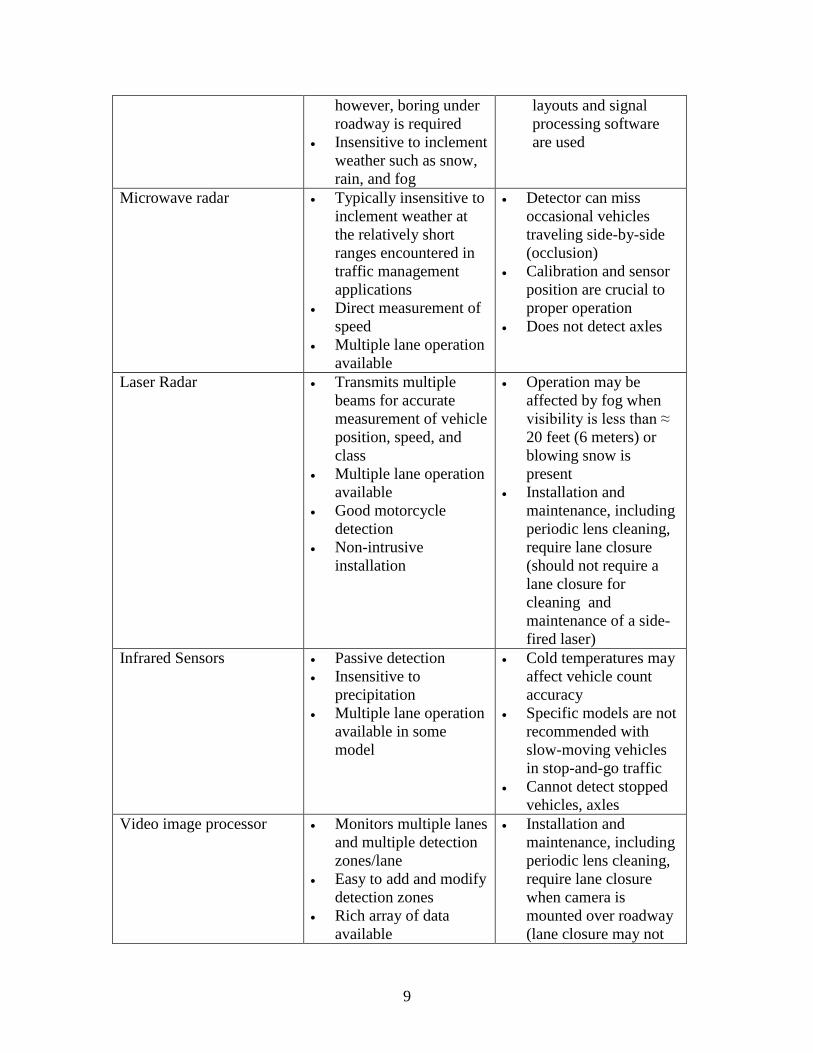
Table 1 compares the strengths and weaknesses of current used detection methods
including installation, data collection, accuracy and maintenance. Some of the sensors are
capable to work above or to the side of the roadway which made installation and
maintenance easier, while most of them need close roadway and pavement cut for
installation. Several technologies are able to support more than 1 lane or multiple
detection zones with limited number of sensors. These devices are good for the places
where need to monitor larger numbers of detection zones.
Table 1 Comparison between Different Methods
Technology Strengths Weaknesses
Inductive loop Flexible design to
satisfy large variety of
applications. Mature,
well understood
technology.
Large experience base.
Provides basic traffic
parameters.
Insensitive to
inclement weather
such as rain, fog, and
snow.
Installation requires
pavement cut. And
improper installation
decreases pavement
life
Installation and
maintenance require
lane closure.
Detection accuracy
may decrease when
design requires
detection of a large
variety of vehicle
classes.
Magnetic Can be used where
loops are not feasible
(e.g., bridge decks)
Some models are
installed under
roadway without need
for pavement cuts;
Installation requires
pavement cut or
boring under roadway
Cannot detect or
classify stopped
vehicles or axles
unless special sensor
9
however, boring under
roadway is required
Insensitive to inclement
weather such as snow,
rain, and fog
layouts and signal
processing software
are used
Microwave radar Typically insensitive to
inclement weather at
the relatively short
ranges encountered in
traffic management
applications
Direct measurement of
speed
Multiple lane operation
available
Detector can miss
occasional vehicles
traveling side-by-side
(occlusion)
Calibration and sensor
position are crucial to
proper operation
Does not detect axles
Laser Radar Transmits multiple
beams for accurate
measurement of vehicle
position, speed, and
class
Multiple lane operation
available
Good motorcycle
detection
Non-intrusive
installation
Operation may be
affected by fog when
visibility is less than ≈
20 feet (6 meters) or
blowing snow is
present
Installation and
maintenance, including
periodic lens cleaning,
require lane closure
(should not require a
lane closure for
cleaning and
maintenance of a side-
fired laser)
Infrared Sensors Passive detection
Insensitive to
precipitation
Multiple lane operation
available in some
model
Cold temperatures may
affect vehicle count
accuracy
Specific models are not
recommended with
slow-moving vehicles
in stop-and-go traffic
Cannot detect stopped
vehicles, axles
Video image processor Monitors multiple lanes
and multiple detection
zones/lane
Easy to add and modify
detection zones
Rich array of data
available
Installation and
maintenance, including
periodic lens cleaning,
require lane closure
when camera is
mounted over roadway
(lane closure may not
10
Generally cost effective
when many detection
zones within the
camera field of view or
specialized data are
required
be required when
camera is mounted at
side of roadway)
Performance affected
by inclement weather
such as fog, rain, and
snow; vehicle shadows;
vehicle projection into
adjacent lanes;
occlusion; day-to-night
transition; vehicle/road
contrast; and water, salt
grime, icicles, and
cobwebs on camera
lens
Reliable nighttime
signal actuation
requires illumination
Requires 30- to 50-ft
(9- to 15-m) camera
mounting height (in a
side-mounting
configuration) for
optimum presence
detection and speed
measurement
Cannot detect axle
Inductive-Loop Detectors: inductive-loop detector can detect vehicles passing or
arriving at certain point. It senses the presences of a conductive metal object by inducing
currents which will reduce the loop inductance. Inductive-loop detectors consist of four
parts: a wire loop installed in the pavement, a lead-in wire connecting pull box with the
wire loop, a lead-in cable connecting the pull box and the controller, and a terminal.
When a vehicle passes over the wire loop or is stopped within the area, it reduces the loop
inductance which results in increasing the oscillator frequency and detected by the
electronic unit and considered as a vehicle.
Magnetic Sensors: magnetic sensors are passive sensors that detect magnetic anomaly
caused by metal in the Earth’s magnetic field. There are two kinds of magnetic field

11
sensors used for traffic monitoring, two-axis fluxgate magnetometer and magnetic
detector. Two-axis fluxgate magnetometer detects changes in both vertical and horizontal
components of the Earth’s magnetic field caused by a ferrous metal vehicle. The
magnetic field sensor referred to as an induction or search coil magnetometer. It detects
the vehicle vibration by monitoring the distortion in the magnetic flux lines induced by
the change in the Earth’s magnetic field produced by a moving vehicle.
Video Image Processor: Video cameras were used for traffic monitoring and analysis
based on their ability to collect vehicle image and transmit to a terminal for operation. A
video image processor typically including more than one cameras, a terminal with
microprocessor-based computer for analyzing the image, and software for interpreting
and transforming them into traffic flow data.
Microwave Radar Sensors: Microware radar was first developed during World War II.
It transmits a continuous wave Doppler waveform to monitor vehicle movement and
provide information of vehicle flow and speed. While it is not able to detect stopped
vehicle. Microwave sensors that transmit a frequency modulated continuous wave are
able to detect both moved and stopped vehicles and provide measurement of vehicle
flow, speed, and occupancy.
Infrared Sensors: Infrared sensors have active and passive types. Active sensors
transmit low power infrared energy laser and collect backward energy laser reflected by
moving vehicles. Passive sensors does not transmit energy of their own. They collect
energy from (1) emitted from vehicles, pavement and other objectives within their view
(2) emitted by the atmosphere and reflected by vehicles, pavement and other objects.

12
Infrared sensors can be used for signal control, occupancy, speed and class measurement;
collect pedestrians movement.
Laser Radar Sensors: Laser radars are active sensor that can transmit energy near the
infrared spectrum. They provide information of vehicle movements, volume, speed,
length and classification. Modern laser sensor can collect 3-D image of vehicle for
classification.
MEMS Accelerometer
An accelerometer is an electromechanical device that measures proper acceleration
forces. These forces could be static or dynamic. Most of the accelerometer is based on the
piezoelectric crystals, but they are too big to be used in some applications (Andrejaši
2008), in this case, researchers developed a smaller and more accuracy sensor using
micro electromechanical systems (MEMS). The first MEMS accelerometer was
developed in 1979 at Stanford University, but it took more than 15 years to be largely
accepted and used (I. Lee 2005). MEMS accelerometers are advanced device that provide
lower power, integrated and accuracy sensing and have huge commercial potential.
Micro Electric Mechanical Systems or MEMS is a term provided around 1989 by
R.Howe (F. Chollet 2008) referred to very small device merges mechanical elements, like
cantilevers or membranes at a nano-scale using micro-fabrication technology. Typically
MEMS components including MicroSensors, MicroActuators, MicroElectronics and
MicroStructures. Microsensors and microactuators work as “transducers” which covert a
measured mechanical signal into an electric signal.
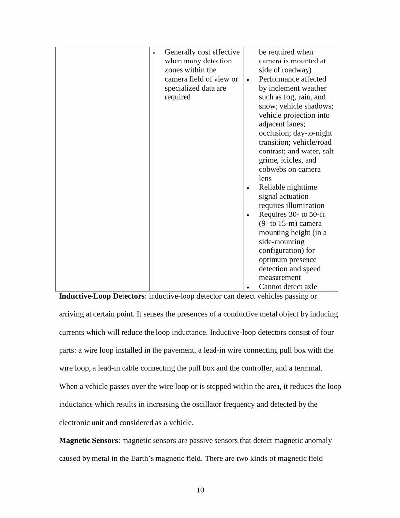
Typical MEMS accelerometer measures acceleration by sensing changes in capacitance.
Capacitive sensing is independent of the material and relies on the geometry of a
13
capacitor. When neglecting the fringing effect near the edge, the parallel-plate
capacitance is (Lyshevski 2002):
(1)
Where A is the area of the electrodes, d is the distance between them and is the
permittivity of the material separating them. Typical structure of MEMS accelerometer is
shown in figure 1, it is composed of moveable proof mass with plates which is attached
to a reference frame using a mechanical suspension system. Moveable plates and fixed
outer plates work as capacitors. By measuring the capacitance changes, the deflection of
proof mass can be detected. The free-space (air) capacitances between the movable plate
and two stationary outer plates and are functions of the corresponding
displacements and :
, (2)
If the acceleration is 0, = so = . The proof mass displacement x corresponding to
the acceleration, if x 0, the capacitance difference is
(3)
Equation 3 can be written to
(4)
For small displacement, is negligible, thus the equation can be simplified to
(5)
It holds true that
(6)

14
Where is output voltage and is input voltage from oscillator. If we use equation 2
and 5, it can be convert to
(7)
For an ideal spring, according to Hook’s law, where is the spring constant.
Also from Newton’s second law of motion, . Thus, the acceleration is
(8)
Then using equation 7, the relationship between acceleration and voltage output is
(9)
Figure 1 Accelerometer Structure (S. E. Lyshevski, Mems and Nems: systems, devices
and structures, CRC Press LLC, USA,2002; Used under fair use, 2014)

15
Accelerometers are being used into more and more personal electric devices like
smartphone which using accelerometers for step counts or tilt sensor for tagging the
photos’ orientation. Accelerometers can also be used in laptop protection when the device
drops suddenly, the accelerometer detects it and switches the hard drive off to avoid
crashing.
In infrastructure health monitoring area, accelerometer can be used to collect pavement or
bridge acceleration to evaluate their health condition. In 2000, Wong et al using
piezoelectric accelerometer to monitor Cable-Supported Bridges in Hong Kong. In 2012,
Kim et al using a capacitive accelerometer to collect vehicle-bridge interaction in
Yeondae Bridge, Korea. With the development of modern electric technology, it becomes
possible that producing highly integrated MEMS board which can be used in different
areas.
Dynamic Loading Analysis
Vehicle loading is commonly considered as static, actually pavement is subjecting to a
moving loading especially when compared with MMLS3 which provides constant
loading to the slab. In this case, it is necessary to do the dynamic loading analysis to
simulate the response under MMLS3. Currently, there are two methods, 2-Dimensional
and 3-Dimensional method, these two method have their own advantages and
shortcomings when using in different conditions.
Two-Dimensional Dynamic Analysis: Sawant conducted 2-D dynamic vehicle–pavement
interaction analysis by idealizing the underlying soil medium with elastic spring and
dashpot systems (without considering the proper continuity between the spring-dashpot
elements) and observed significant effect of velocity of moving load on pavement

16
response. The dynamic interaction between the moving load and the pavement was
considered by modelling the vehicle by spring–dashpot unit. Sawant et al. conducted 2-D
finite element analysis of rigid pavements under moving vehicular or aircraft loads. The
analysis was based on the classical theory of finite thick plates resting on two-parameter
elastic soil medium. However, the infinite plate elements were not included in the
solution algorithm and also a proper study was not being conducted to investigate the
effect of vehicle–pavement interaction on the dynamic response of rigid pavement.
Huang and Thambiratnam proposed a procedure to investigate the dynamic behavior of
the rectangular plate resting on an elastic Winkler foundation subjected to moving loads.
They used the finite strip method and a spring system and showed that the velocity of
moving load and elastic foundation stiffness have significant effects on the dynamic
response of the plate.
Three-Dimensional Dynamic Analysis: To accomplish a comprehensive analysis of
pavement behavior incorporating the pavement-soil interaction effects, it is necessary to
model the pavement in the form of 3D elements and the supporting soil medium as 3D
elastic continuum. In general, there are two important factors that should be considered in
any dynamic pavement analysis: (1) The variation of the interaction load with time and
space; and (2) the dependency of the material properties on the applied stress and the
loading frequency.
Zaghloul and White considered several realistic conditions of the flexible pavement
problem and using ABAQUS as an analysis tool. 3D analysis was used in which the
asphalt concrete was considered viscoelastic, the base was treated by Drucker–Prager
model and the subgrade by CamClay model. The load was simulated as a moving load. In
17
their model sensitivity analysis, they investigated the effect of deep foundation type,
some other attributes of the pavement cross section, and the dynamic features of the
traffic load on the pavement rutting. The results of surface deflection were correlated to
the surface deflection results of the elastic analysis. Ioannides and Donnelly used the 3D
models to simulate pavement problems concerning the effect of subgrade stress
dependence. Wu and Shen presented the dynamic analysis of rigid pavements by
modeling the pavement as 3D brick elements supported by spring and dashpots.
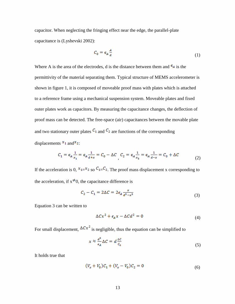
Uddin and Ricalde successfully implemented microcraking and crack propagation models
into ABAQUS (with the help of the feature of user-defined subroutines) to simulate the
viscoelasticity of the asphalt concrete layer. In their work, the pavement foundation was
considered linear elastic, and 3D dynamic analyses were adopted.
Bassam et al using 3D dynamic FE analyses considering the granular base as elastic
perfectly plastic (Druker–Prager) and the subgrade as elastoplastic strain hardening (Cam
Clay) are carried out to investigate the effect of base thickness, base quality, and the
subgrade quality on the fatigue of the pavement system, reflected by the maximum tensile
strain at the bottom of asphalt concrete layer.
Al-Qadi et al developed a 3-D finite element model to predict the pavement responses to
vehicular loading. The model was verified with in situ pavement responses to accelerated
pavement loading. In their model, the measured 3-D tire–pavement contact stresses on a
flat pavement are considered in the 3-D FE modeling. Hence, the dynamic loads would be
simplified by the continuous changing of the loading amplitude within the tire–pavement
contact area.
Comparison between 3D Analysis and 2D Analysis

18
Despite the fact that it requires considerably more computational time and computer
memory, the 3D analysis is still considered superior to the 2D analysis. The necessity for
adopting the 3D analysis arises from the following advantages.
1. It better reflects the complex behavior of the composite pavement system materials
under traffic loads of different configurations.
2. It is preferred when verifying numerical model results with the laboratory or field test
results.
3. It is capable of simulating the rectangular footprint of the loaded wheel In other words,
when dealing with 2D analysis, the load shape is restricted to a circular (axisymmetric
condition) or infinite strip load (plane strain condition), which is not realistic.
Summary of Findings
With an accuracy vehicle classification method, engineers can design a better
maintenance programs, evaluate highway usage and plan the future development
strategies. The vehicle-pavement interaction can be detected by accelerometer to classify
vehicles. Currently, the vast majority accelerometers are based on piezoelectric crystal,
however, they are too big and clumsy to be used in specific areas. In this case,
researchers developed a more integrated and much smaller MEMS accelerometer. While
in pavement monitoring area, it have not been used very often probability due to its
higher cost. Traditional sensor installation needs pavement cut-off which will shorten the
lifespan of the pavement, in other words, it will cause higher maintenance cost to ensure
pavement serviceability. Also the device subjects to the traffic loading which will cause
the device broken easily. To find a balance between cost and monitor efficiency, a

19
MEMS accelerometer installed beside pavement without subjecting to the traffic directly
need to be considered. Pavement acceleration has not been much considered to monitor
the health condition, and less researches have been done about the pavement acceleration
under different conditions. In this case, it is real necessary to do the tests about the
pavement response when it in a good or bad condition. At the same time, the simulation
using dynamic analysis to verify the laboratory tests results is important too.
20
3. Laboratory Tests Using MMLS3
Before applying our sensor to the pavement, series laboratory tests were done to verify
the feasibility and accuracy of the accelerometer monitor the wheel passing. A MMLS3
machine was used to simulate the actual traffic situation. Sensor was attached to the
asphalt plate just next to the wheel. Four different speeds were conducted to test sensor
reaction to different traffic conditions. Acceleration data was recorded by the sensor and
transmitted to laptop through USB cable.
MEMS Accelerometer Selection
An Omega CP-Ultrashock-50 Tri-axial Shock Recorder with MEMS semiconductor to
collect pavement acceleration data. It is a battery powered, stand alone and easy-installed
sensor which also has a strong resistance to the outside environment influence. Its
acceleration range is up to ±250 g and the calibration accuracy is about ±0.2 g, the
recording interval is 64Hz.
Experiment Setup
To simulate actual traffic condition, laboratory tests using MMLS3 were applied to our
MEMS accelerometer to verify the accuracy. Sensor was fixed to the asphalt plate using
expansion screws, so that the sensor could vibrate with pavement. It located on the edge
of the plate next to wheels without subjecting to the loading which also simulated our
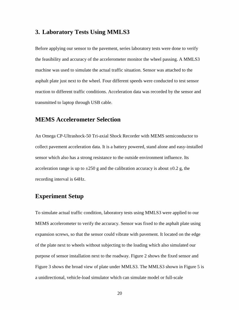
purpose of sensor installation next to the roadway. Figure 2 shows the fixed sensor and
Figure 3 shows the broad view of plate under MMLS3. The MMLS3 shown in Figure 5 is
a unidirectional, vehicle-load simulator which can simulate model or full-scale

21
accelerated traffic under both dry and wet condition. The MMLS3 device is 2.4 m (7.9
ft.) long by 0.6 m (2 ft.) wide by 1.2 m (3.9 ft.) high. This Accelerated Pavement Testing
device has pneumatic tires which are 3/10 or approximately one-third the diameter of
standard truck tires and apply a load on 300 mm (12 in) diameter. The MMLS3 has four
wheels with a distance between centerlines of 1.05 m (3.4 ft.). It can provide up to 2.7
kN (607lbs or approximately one-ninth of the load on one wheel of a dual tire standard
single axle) when simulate the traffic on pavement. A maximum of 7200 single-wheel
load repetitions can be applied per hour at a speed of up to 2.6 m/sec (8.5 ft. /sec) that
corresponds approximately to a 4 Hz frequency of loading for a measured tread length of
0.11 m (0.36 ft.) (de Fourtier Smit 1999).
Figure 2 Sensor Fixed to the Plate
22
Figure 3 Broad View of the Plate
To simulate real traffic situation and verify sensor sensitivity under different conditions,
four different speeds (10, 20, 30, and 40) were applied. Wheel passes were recorded
manually during every tests, so that can be compared with calculated axle count based on
our output signal. Output data was collected by the Omega software through USB cable
after the test was finished.
23
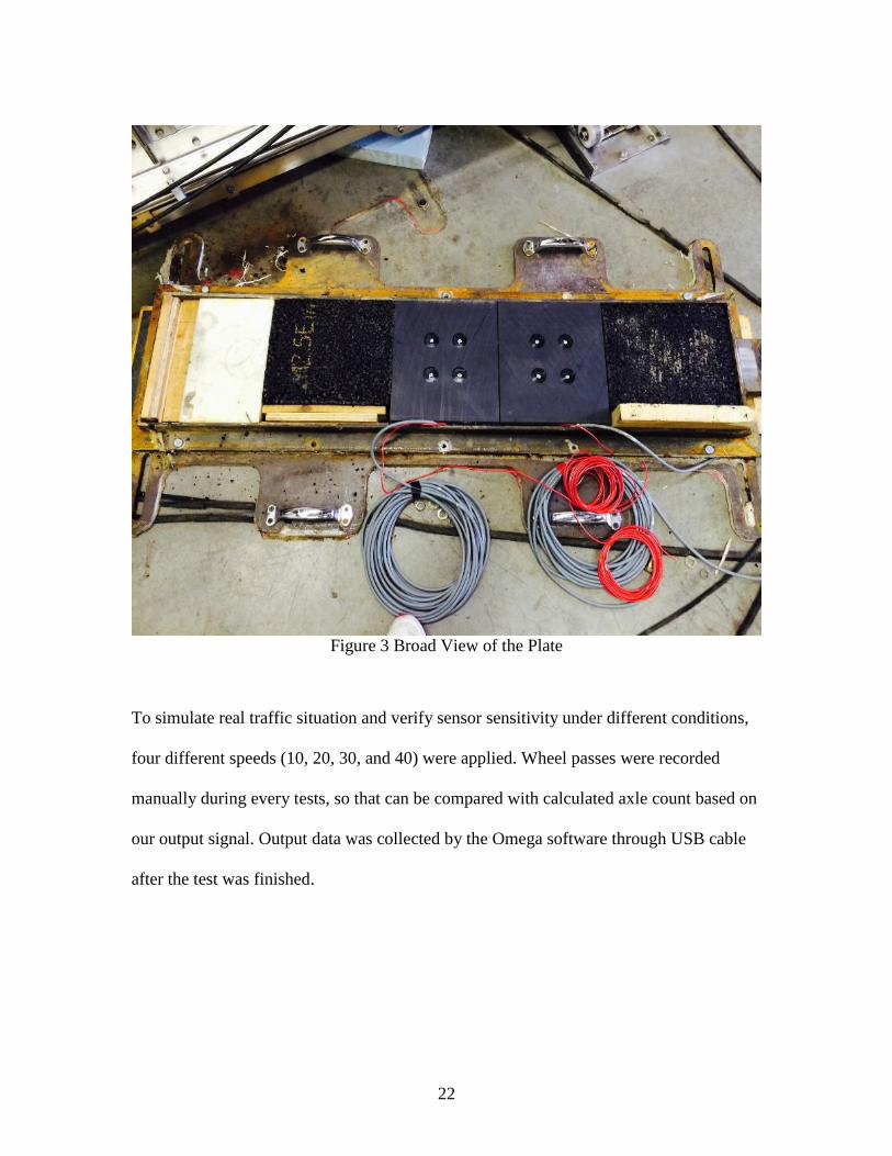
Figure 4 Slab with a Crack
To test the reaction of bad surface condition, a one inch wide 1.5 inches deep crack was
created just beneath the sensor.

24
Figure 5 Broad View of MMLS3
Test Procedures
Pavement Acceleration Tests
Once the sensor installed on the asphalt plate, it can be connected with personal computer
using USB cable and controlled by OM Data Logger Software. To collect data, the
software has to be open first and wake up the sensor by pushing start button, then it can
collect pavement vibration while MMLS3 is running.
When the test is running, number of wheel passing the sensor has to be recorded
manually. During the test, make sure that wheel loading is the only source for the
pavement vibration.

25
Once the test finished, stop the sensor and download data to personal computer through
the software, the download data was saved as an .mtff file including 3-axle acceleration
and temperature, humanity and pressure. Since the purpose was to classify the vehicle
and tests environment almost keep constant, only 3-axle acceleration data was exported
and analyzed. Figure 6 shows the interface and output data of the software.
Figure 6 Interface of the Software
26
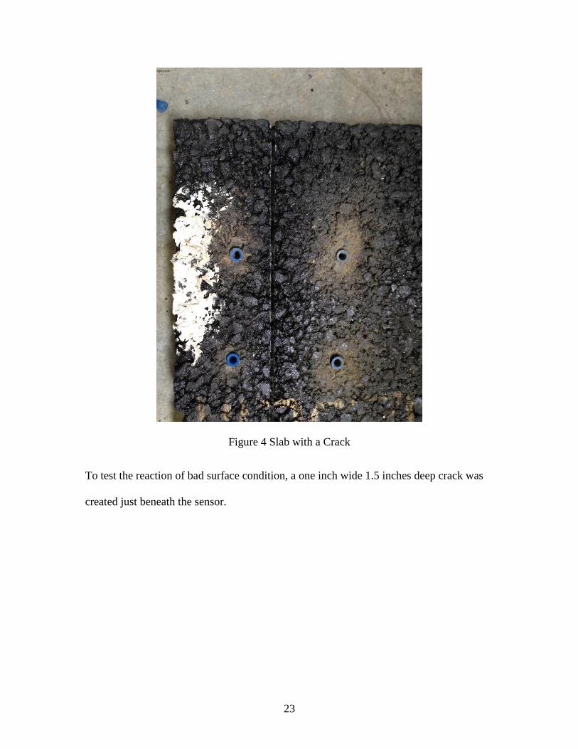
Figure 7 Flow Chart of Test Procedures
MMLS3 Speed Tests
Since the speed provided by MMLS3 does not use the common unit and increases non-
linearly, speed correction is necessary for the further verification.
Distance between wheel centerline given by manufacturer is 1.05m (41 inch), when we
record the time X of running Y cycles, speed could be calculated as
in/s
In our tests, time spent of 50, 75, 100, 125 cycles has been recorded, and the calculated
speeds are listed below:
Table 2 Correction Speed
MMLS3 Speed Correction Speed (in/sec)
10 17.52137
20 36.18148
30 54.78869
40 72.1831

27
4. Dynamic Loading Simulation
Necessity of Using Dynamic Analysis
When considering the small traffic flow, low speed and light load, the linear elastic
theory with static loads was adopted. Pavement dynamic responses may be larger than
static responses and exacerbate pavement distresses. Therefore, when pavement dynamic
responses are considered, the reliability and durability of pavement structure would be
sufficiently evaluated. Along with the development of computational mechanic, the finite
element method and the boundary element method broke the limitations of boundary
conditions and load types in analytical methods. In our laboratory tests, the highest speed
is about 72 in/sec which could be considered as a low speed loading, at the same time, the
wheel passing is constant in MMLS3, in this case, dynamic analysis using finite element
method gave us a straightforward view to monitor the pavement vibration and compare it
with our sensor results.
Finite Element Model Geometry
To simulate the slab vibration with and without crack under MMLS3, ABAQUS Version
6.13 was used based on dynamic loading analysis. Since the slab size tested was fixed,
the modeled domain is the same as the slab which is 12 inches long, 10.5 inches wide and
1.5 inch thick. Figure 8 is the 3-D finite element slab domain without a crack. The whole
slab was divided into 1512 elements each is 0.5*0.5*0.5 inch.

28
Figure 8 3-D Model of Slab without Crack
To create the model of slab with a crack, we did it into two parts separated by the crack
which shown in Figure 9. In this case, the boundary condition at the crack location is
different from other point where a roller support condition will be used.
29
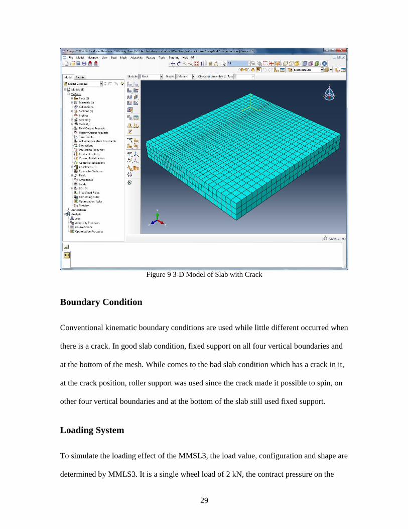
Figure 9 3-D Model of Slab with Crack
Boundary Condition
Conventional kinematic boundary conditions are used while little different occurred when
there is a crack. In good slab condition, fixed support on all four vertical boundaries and
at the bottom of the mesh. While comes to the bad slab condition which has a crack in it,
at the crack position, roller support was used since the crack made it possible to spin, on
other four vertical boundaries and at the bottom of the slab still used fixed support.
Loading System
To simulate the loading effect of the MMSL3, the load value, configuration and shape are
determined by MMLS3. It is a single wheel load of 2 kN, the contract pressure on the

30
slab is assumed to be the same as tire pressure which is 800 kPa in this analysis. Since
four different speeds were applied on the slab, the loading frequency changed among
different speeds. The distance between centerline of each wheel is 3.4 ft, and loading
frequency could be easily decided by distance/speed.
31
5. Experimental and Simulation Results Analysis
Axle Detection Algorithm
Based on Ravneet Bajwa et al. work, every moving wheel can be modeled as a moving
impulsive force on the pavement. In this case, it can cause vibration of pavement together
with sensor so that the acceleration could be recorded. It would be easy to spot different
axles from our sensor signal if they have obvious differences in time, for example, the
next axle arrives sensor when the whole decay of the last axle’s signal. However, the
actual highway traffic has a more complicit situation.
So a statistical method is needed to efficiently detect vehicle axle from sensor output
signal. An appropriate approach can still filter axle form signal even moderate overlap
exists. Our algorithm is based on the Ravneet Bajwa et al method and has been improved
to fit our project.
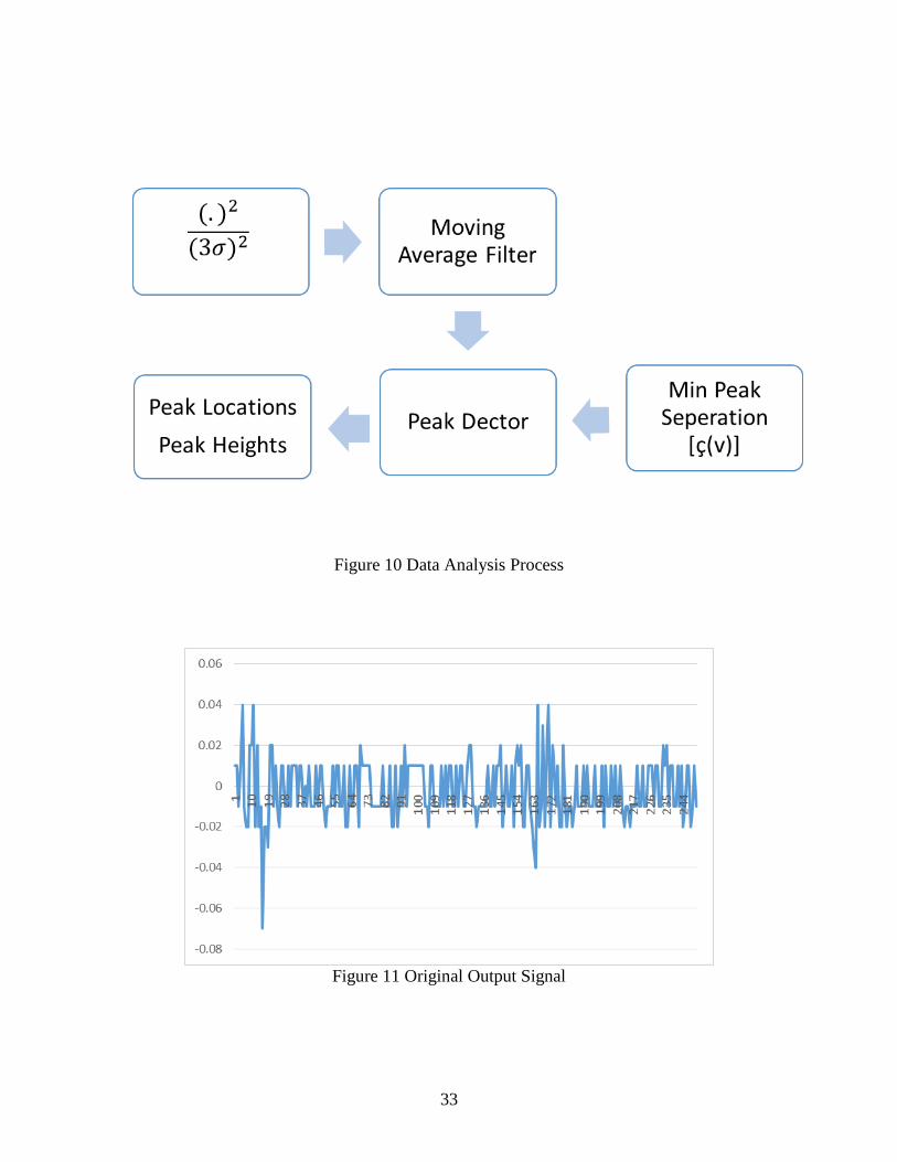
Figure 10 shows the block diagram of signal analysis. It attenuates noise and amplifies
useful signal, finally locates the peaks that are separated in time. Figure 11 shows part of
the output signal form our sensor. It is hard to tell noise and axle signal from it, so the
statistical method is important to spot axle and minimize noise. The signal a(n) is divided
by 3 times the noise (given by sensor manufacture). This step ensures that signal without
wheel loading is below 1. After that, the signal is squared to get the energy, this step
further attenuates the noise and amplifies the useful signal which is greater than 1. Figure
12 is the signal chart after the first step. In this figure, noise has been attenuated and
ranged between a very limited values, at the same time, several peaks are clearly appears.
32
The next step is passing the signal through a Moving Average Filter so that the signal
could be smoothed and easily find their peaks. M(v) is the number of points in the
average which determines the bandwidth of the filter, and the bandwidth need to be speed
based. From other researches did before, the bandwidth is empirically defined
as . In our laboratory tests, according to our MMLS3 running speed and
actual traffic condition, 50 mph is used so that the filter tap is 18. This step further
smoothed our signal and spotted signal peaks more effectively. Figure 13 is the signal
chart after passing the moving average filter. In this figure, three peaks are clearly
spotted.
The last step helps to filter peaks in the smoothed signal with a minimum time separation
(ç (v)). This step ensures that local variations near peaks are not considered as an axle. In
this case, space distance determines the time separation. In laboratory tests, distance
between MMLS3 wheel centerline is about 42 inch, so assuming that axles are at least 40
inch apart. When applied to the actual vehicle situation, different axle distance has to be
considered, typically, 6 ft is reasonable for time separation. If tandem axle which mostly
consider as one axle want to be detected separately, 4 or 5 ft may be selected for the time
separation.
33
Figure 10 Data Analysis Process
Figure 11 Original Output Signal
34
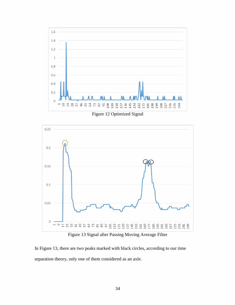
Figure 12 Optimized Signal
Figure 13 Signal after Passing Moving Average Filter
In Figure 13, there are two peaks marked with black circles, according to our time
separation theory, only one of them considered as an axle.

35
Axle Spacing and Speed Estimation
According to the product specification, it has a 64 Hz recording interval which means it
records data every 0.015s, so every unit in the figure counts as 0.015s. From output
signal, refers to the peak time of axle a. In laboratory tests, as calculated before, the
speed of MMLS3 is known and the axle spacing between axles a and a+1 can be
determined as
On the other hand, the wheel spacing of MMLS3 is also known as s, the speed can be
calculated as
v=s/ ( )
Since the speed of wheel and the wheel centerline distance are both known in our
laboratory tests, given any one of them can help to determine another one, in this case,
we can verify the accuracy of sensor for detecting speed and axle spacing which will be
explained later.
Experimental Results and Verification
One of the most important tasks in these research is to detect axle which reflects as a
peak in output signal so that vehicle classification can be done. Sensor used in our test is
a 3-axle accelerometer which has x, y and z-axle vibration data and all of them were
analyzed to see the different and find out a better source for vehicle classification.

36
Sensor Performance
The noise of the sensor when there is no wheel passing was measured and listed below.
Table 3 Noise RMS and Signal Amplitude
Noise RMS Signal Amplitude
X-Axle 0.000131 >0.05
Y-Axle 5.477E-5 >0.1
Z-Axle 0.504 >1
According to our comparison between noise RMS and signal amplitude, x and y-axle
have significant higher output than the noise while z-axle shows a slightly difference.
However, the absolute value of z-axle accelerometer is greater than other two axles, the
reason that causes little different between sensor noise and collect accelerometer is
probably applied loading is not heavy enough.
Figure 14 OM-CP-ULTRASHOCK-5 Shock Recorder Channel 4 Shock - X Axis (g)
37
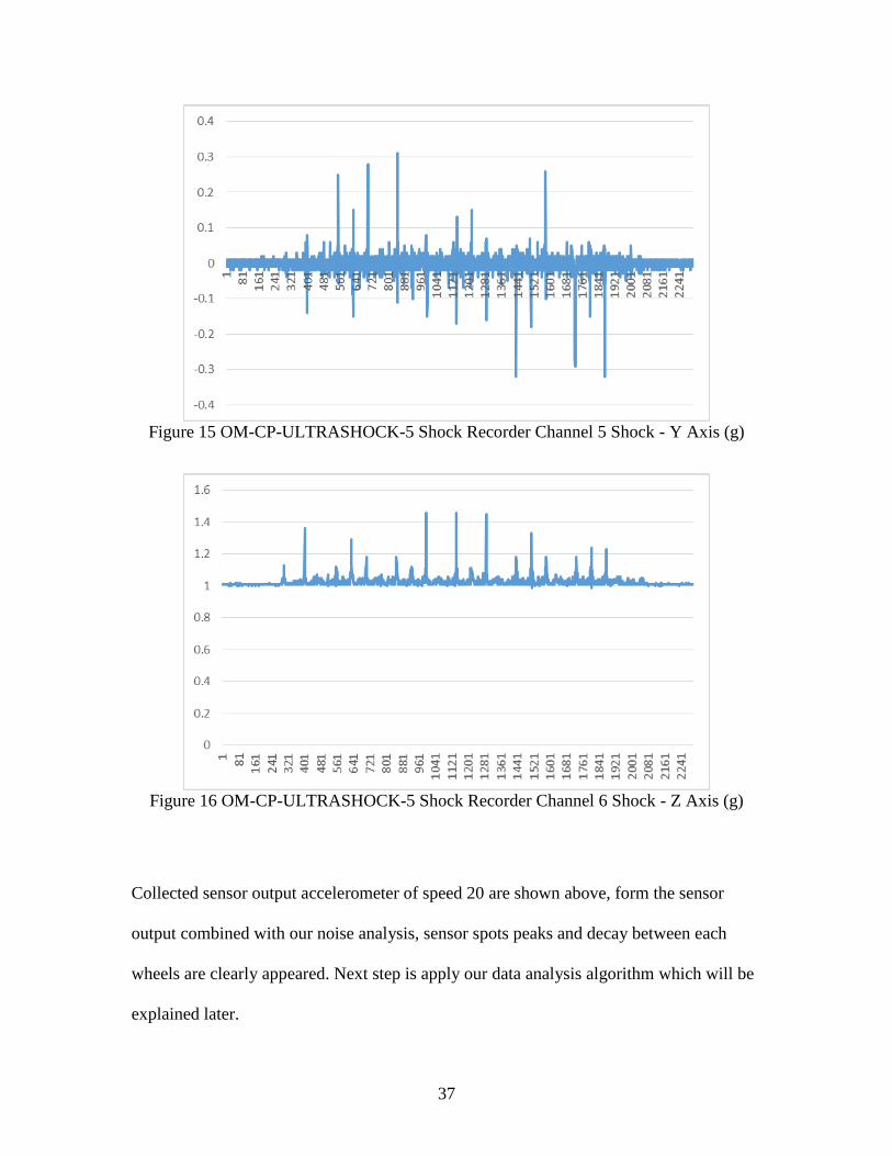
Figure 15 OM-CP-ULTRASHOCK-5 Shock Recorder Channel 5 Shock - Y Axis (g)
Figure 16 OM-CP-ULTRASHOCK-5 Shock Recorder Channel 6 Shock - Z Axis (g)
Collected sensor output accelerometer of speed 20 are shown above, form the sensor
output combined with our noise analysis, sensor spots peaks and decay between each
wheels are clearly appeared. Next step is apply our data analysis algorithm which will be
explained later.
38
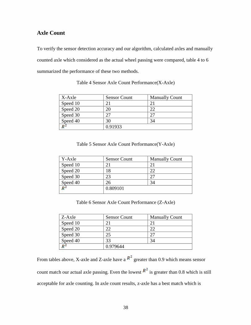
Axle Count
To verify the sensor detection accuracy and our algorithm, calculated axles and manually
counted axle which considered as the actual wheel passing were compared, table 4 to 6
summarized the performance of these two methods.
Table 4 Sensor Axle Count Performance(X-Axle)
X-Axle Sensor Count Manually Count
Speed 10 21 21
Speed 20 20 22
Speed 30 27 27
Speed 40 30 34
0.91933
Table 5 Sensor Axle Count Performance(Y-Axle)
Y-Axle Sensor Count Manually Count
Speed 10 21 21
Speed 20 18 22
Speed 30 23 27
Speed 40 26 34
0.809101
Table 6 Sensor Axle Count Performance (Z-Axle)
Z-Axle Sensor Count Manually Count
Speed 10 21 21
Speed 20 22 22
Speed 30 25 27
Speed 40 33 34
0.979644
From tables above, X-axle and Z-axle have a greater than 0.9 which means sensor
count match our actual axle passing. Even the lowest is greater than 0.8 which is still
acceptable for axle counting. In axle count results, z-axle has a best match which is
39
reasonable that when wheel pass by the sensor, the vibration on the vertical direction
should be strongest, this theory also supported by our actual pavement tests.
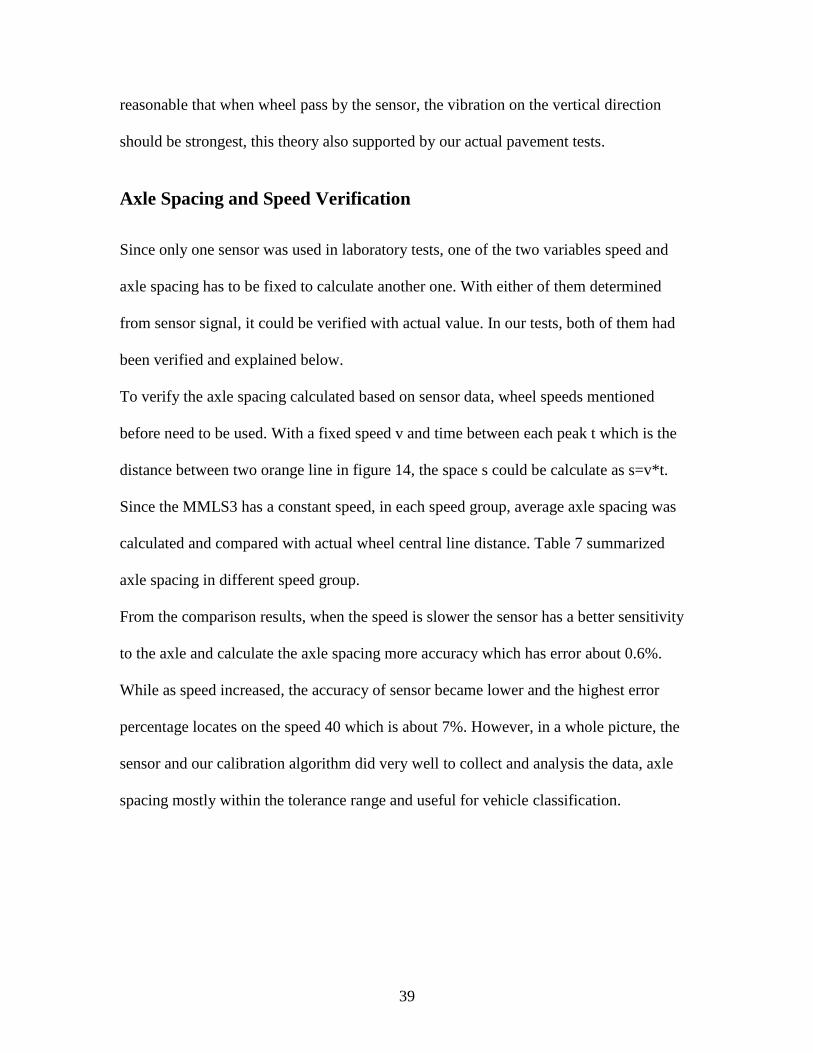
Axle Spacing and Speed Verification
Since only one sensor was used in laboratory tests, one of the two variables speed and
axle spacing has to be fixed to calculate another one. With either of them determined
from sensor signal, it could be verified with actual value. In our tests, both of them had
been verified and explained below.
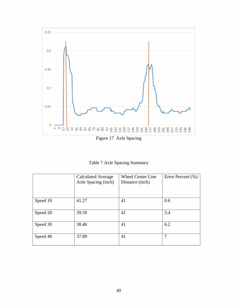
To verify the axle spacing calculated based on sensor data, wheel speeds mentioned
before need to be used. With a fixed speed v and time between each peak t which is the
distance between two orange line in figure 14, the space s could be calculate as s=v*t.
Since the MMLS3 has a constant speed, in each speed group, average axle spacing was
calculated and compared with actual wheel central line distance. Table 7 summarized
axle spacing in different speed group.
From the comparison results, when the speed is slower the sensor has a better sensitivity
to the axle and calculate the axle spacing more accuracy which has error about 0.6%.
While as speed increased, the accuracy of sensor became lower and the highest error
percentage locates on the speed 40 which is about 7%. However, in a whole picture, the
sensor and our calibration algorithm did very well to collect and analysis the data, axle
spacing mostly within the tolerance range and useful for vehicle classification.
40
Figure 17 Axle Spacing
Table 7 Axle Spacing Summary
Calculated Average
Axle Spacing (inch)
Wheel Center Line
Distance (inch)
Error Percent (%)
Speed 10 41.27 41 0.6
Speed 20 39.59 41 3.4
Speed 30 38.46 41 6.2
Speed 40 37.89 41 7
41
Table 8 Speed Verification Summary
MMLS3
Display Speed
Correction Speed (in/sec) Speed Calculated
According to Sensor
Signal (in/sec)
Error
Percentage
10 17.52137 17.40 0.6
20 36.18148 36.50 0.9
30 54.78869 58.40 6.5
40 72.1831 75.09 4.0
When using a fixed axle spacing which is the wheel center line distance to calculate the
speed and compare with our correction speed, it could tell the accuracy of our sensor and
calculation algorithm. Table 8 listed the correction speed and speed calculated based on
sensor output data. According to the results, our calculated speeds are almost the same as
the correction speed, the highest error is about 6.5% which is still within the tolerance
range.
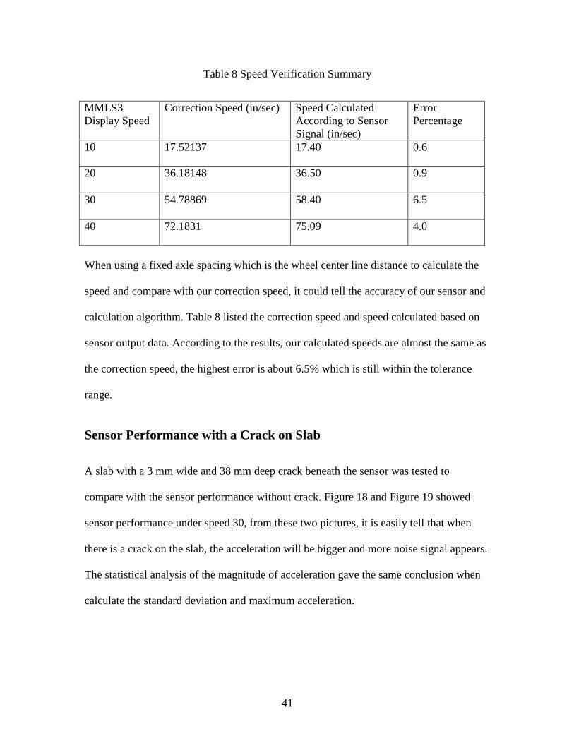
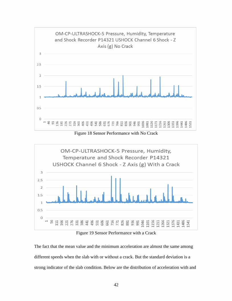
Sensor Performance with a Crack on Slab
A slab with a 3 mm wide and 38 mm deep crack beneath the sensor was tested to
compare with the sensor performance without crack. Figure 18 and Figure 19 showed
sensor performance under speed 30, from these two pictures, it is easily tell that when
there is a crack on the slab, the acceleration will be bigger and more noise signal appears.
The statistical analysis of the magnitude of acceleration gave the same conclusion when
calculate the standard deviation and maximum acceleration.
42
Figure 18 Sensor Performance with No Crack
Figure 19 Sensor Performance with a Crack
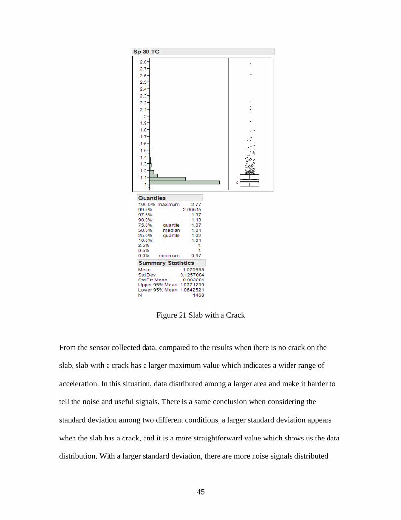
The fact that the mean value and the minimum acceleration are almost the same among
different speeds when the slab with or without a crack. But the standard deviation is a
strong indicator of the slab condition. Below are the distribution of acceleration with and

43
without a crack when speed is 30. The standard deviation of the acceleration for the better
slab condition is about 0.06g, while the standard deviation for the slab with a crack is
0.126g which is about two times than the good condition. From Table, we have a same
conclusion whatever the speed is. Also from the table, as the speed increases, the
standard deviation increases as well.
Table 9 Standard Deviation Comparison
Speed Crack Non-Crack
10 0.01709 0.009538
20 0.060055 0.033347
30 0.125708 0.059857
40 0.100644 0.053885

44
Figure 20 Slab without Crack
45
Figure 21 Slab with a Crack
From the sensor collected data, compared to the results when there is no crack on the
slab, slab with a crack has a larger maximum value which indicates a wider range of
acceleration. In this situation, data distributed among a larger area and make it harder to
tell the noise and useful signals. There is a same conclusion when considering the
standard deviation among two different conditions, a larger standard deviation appears
when the slab has a crack, and it is a more straightforward value which shows us the data
distribution. With a larger standard deviation, there are more noise signals distributed
46
along the actual peak location which will reduce the accuracy of detecting the wheel
passing.
Simulation Results Analysis
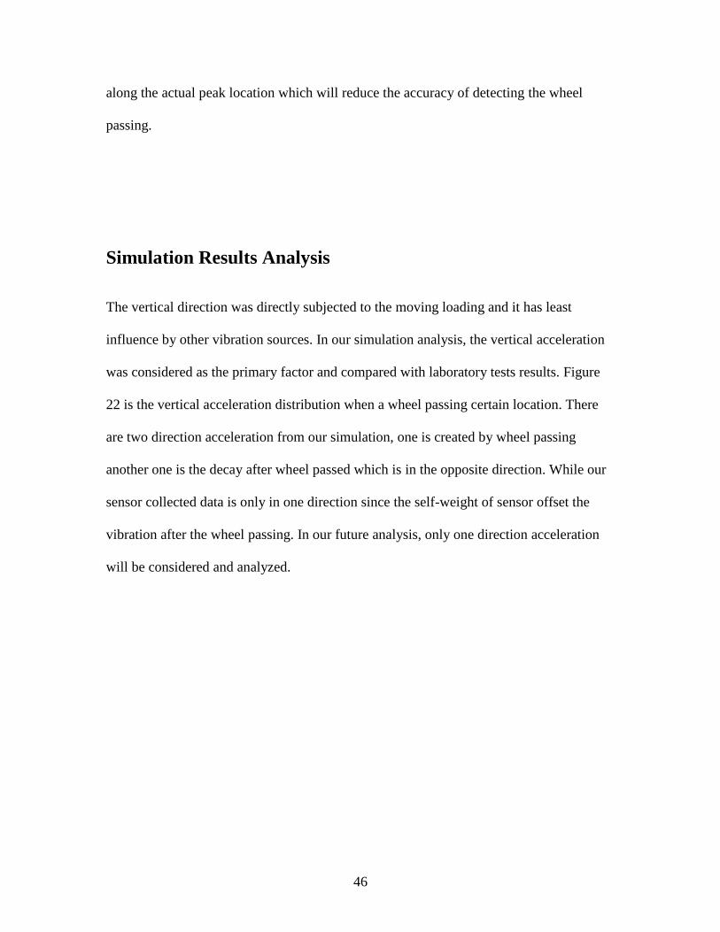
The vertical direction was directly subjected to the moving loading and it has least
influence by other vibration sources. In our simulation analysis, the vertical acceleration
was considered as the primary factor and compared with laboratory tests results. Figure
22 is the vertical acceleration distribution when a wheel passing certain location. There
are two direction acceleration from our simulation, one is created by wheel passing
another one is the decay after wheel passed which is in the opposite direction. While our
sensor collected data is only in one direction since the self-weight of sensor offset the
vibration after the wheel passing. In our future analysis, only one direction acceleration
will be considered and analyzed.
47
Figure 22 Vertical Acceleration
Simulation Results without Crack
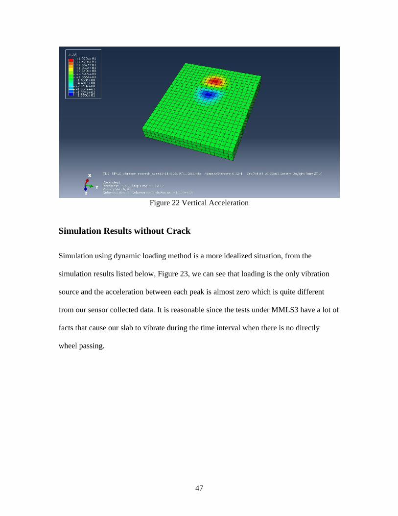
Simulation using dynamic loading method is a more idealized situation, from the
simulation results listed below, Figure 23, we can see that loading is the only vibration
source and the acceleration between each peak is almost zero which is quite different
from our sensor collected data. It is reasonable since the tests under MMLS3 have a lot of
facts that cause our slab to vibrate during the time interval when there is no directly
wheel passing.
48
Figure 23 Simulation Results of Acceleration
But when we look detail into the certain period when the wheel loading is the primary
vibration source, both the laboratory tests and simulation results have better match to
each other. A single wheel passing was selected and compared below. Both of the
simulation and sensor represented a peak value for a wheel passing. Compare to sensor
collected data, the simulation results show a more sensitive response to the wheel
passing, before the wheel arrived the recording point, there are vibrations at the recording
point. While the sensor had less reaction to it since the sensor its weight which offset this
vibration. This also explained the sensor signal decayed faster than the simulation, due to
the sensor weight, it forced sensor back to its original position and offset the vibration
from wheel passing.

49
Figure 24 Single Wheel-Passing Comparison between Sensor and Simulation
Simulation Results with a Crack
To estimate the influence of pavement condition to the vibration, a simulation of slab
reaction to the wheeling passing with a crack in it was conducted and compared with
laboratory tests.
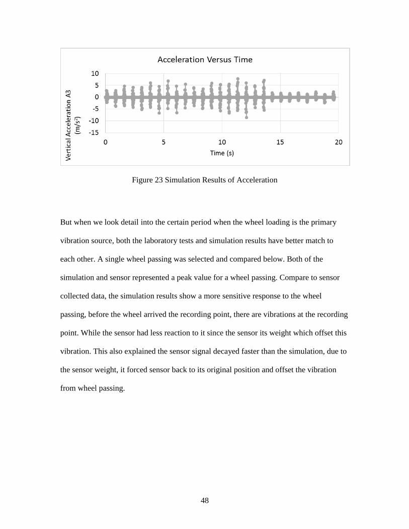
Figure 25 is the simulation results of a slab with a crack in it. The maximum acceleration
is about 3 times larger than the slab in a good condition. Compared to the sensor data, the
simulation results are more accuracy since the wheel passing is the only vibration source.
In our laboratory tests, other factors like machine vibration would influence the actual
vibration of the slab.
50
Figure 25 Simulation Results of Acceleration
But when we look detail into the single peak which represents a wheel passing and
compare it with our labortoray results, shown in Figure 26, they are very similar to each
other since the wheel passing is the primary vibartion source.
However, with a crack in the slab, around sensor collected peak location, our simulation
results have more than one peaks. In this case, other peasks will decrease the accuracy
detecting the actual wheel passing. From the figure we can also see that, after the wheel
passing, the accelaration decay is much slower than the no crack condition, some
vibrations even exist few seconds after the peak.
51
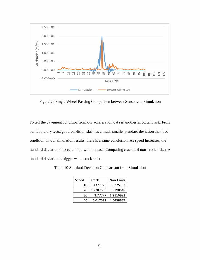
Figure 26 Single Wheel-Passing Comparison between Sensor and Simulation
To tell the pavement condition from our acceleration data is another important task. From
our laboratory tests, good condition slab has a much smaller standard deviation than bad
condition. In our simulation results, there is a same conclusion. As speed increases, the
standard deviation of acceleration will increase. Comparing crack and non-crack slab, the
standard deviation is bigger when crack exist.
Table 10 Standard Devotion Comparison from Simulation
Speed Crack Non-Crack
10 1.1377926 0.225157
20 1.7782633 0.298548
30 3.77777 1.2116992
40 5.617622 4.5438817
52
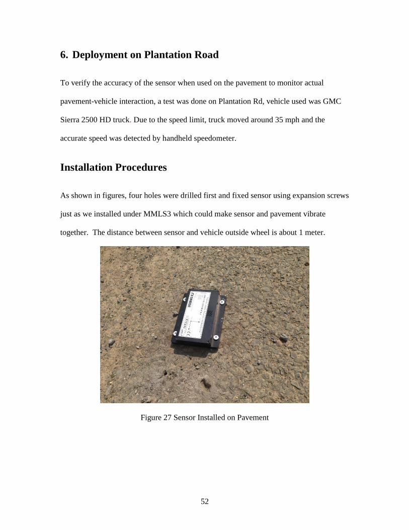
6. Deployment on Plantation Road
To verify the accuracy of the sensor when used on the pavement to monitor actual
pavement-vehicle interaction, a test was done on Plantation Rd, vehicle used was GMC
Sierra 2500 HD truck. Due to the speed limit, truck moved around 35 mph and the
accurate speed was detected by handheld speedometer.
Installation Procedures
As shown in figures, four holes were drilled first and fixed sensor using expansion screws
just as we installed under MMLS3 which could make sensor and pavement vibrate
together. The distance between sensor and vehicle outside wheel is about 1 meter.
Figure 27 Sensor Installed on Pavement

53
Figure 28 Sensor Location on Pavement
Test Results and Analysis
Z-axle acceleration was used for analyzed since it had a better sensitive to the vehicle-
pavement interaction. The same algorithm was used in processing the data.
The noise of static sensor were tested first, from the output results, the noise keeps at a
constant value. Compared with laboratory test noises, pavement noise seems stable and
easy to tell, in this case, an easy step could be used to analyze our output signals to detect
axles.
Since the actual pavement noise locates between a certain values, after filter those noise
within that range, the useful signal could appear clearly. Figure 29 shows the original
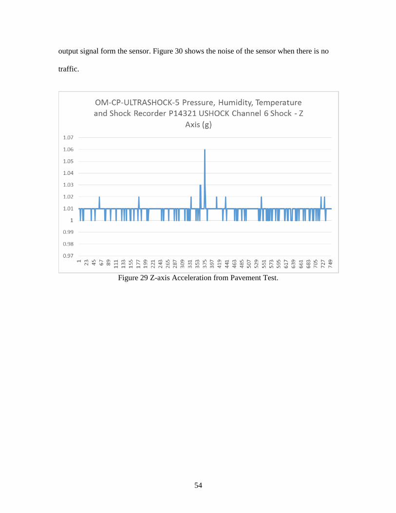
54
output signal form the sensor. Figure 30 shows the noise of the sensor when there is no
traffic.
Figure 29 Z-axis Acceleration from Pavement Test.

55
Figure 30 Static Noise Signal
Figure 31 Optimized Signal

56
From the figures 31, two peaks are clearly appeared which reflect as two axles.
According to the actual condition, the truck used for our experiment has two axle just as
our sensor monitored.
Time interval between two peaks were calculated as 0.195 sec. the speed detected by
handed speedometer was 35 mph. So the axle spacing monitored by sensor was 10 feet.
The official wheelbase given by GMC is 11.14 feet. The error rate is only about 1%
which is accurate for vehicle classification.
Due to the limitation of field, only one kind of truck was tested and only 35 mph was
applied. Higher speed cannot be tested because of the speed limitation. In the future,
more kinds of vehicles and more speeds may be conducted. However, the test results
were quite well and prove the feasibility of using MEMS accelerometer for vehicle
classification.
57
7. Conclusions and Future Work
Vehicle Classification Based on MEMS Accelerometer
The first object of this project was to verify the feasibility of using MEMS accelerometer
to classify vehicle based on axle count and spacing. A laboratory test was designed,
conducted and applied to pavement. MMLS3 was used during the laboratory test to apply
four different speeds to see the reaction of sensor. From output signal, the sensor had a
good reaction to the wheel-pavement interaction, almost every axle passing showed a
peak on the signal. The installation compared to existing methods has many advantages,
since it located beside the pavement which without subjecting to the traffic loading
directly will have a long-lifespan than traditional technologies. Also, this non-destructive
method without cutting the pavement will protect the pavement form potential damage
caused by improper installation. The data collection will be convenient and safe for
engineers because they do not need to close traffic lanes or enter lanes. The laboratory
test certify the feasibility of using MEMS accelerometer for vehicle classification.
The second object was to develop an algorithm to analysis the test data. The algorithm
including a moving average smoothing filter and peak detector that could successfully
locate every axle and report the time interval between two axles. The lowest error rate of
this algorithm could be 0.7% for spacing and 0.6 % for speed calculation which are quite
satisfactory. This method also used on the pavement test and output an accuracy axle
detection result which could be easily used for vehicle classification.
Since all the tests did under relative low speed condition compared to actual traffic, also
form our results, the accuracy has a decreasing trend as speed increases, in the future,
58
sensor will be installed beside a local highway to see the reaction. In our project, only one
sensor was used to monitor the vehicle-pavement reaction, so we have to fix one variable
to verify another. For example, when we want to know the accuracy of calculating the
axle space, speed has to be fixed. In the future test, more sensors could be used, once the
distance between each sensor is known, either speed or spacing can be calculated through
sensor output data.
Currently, we have not considered the multi-lane condition whether the vehicle vibration
on the further lanes could be collected by the sensor or the vibration from other lanes may
affect the signal collection. A better way to avoid this is installed on a weigh station
where only one lane open to trucks so that an accuracy signal could be collected.
Even though the installation and data collection method are more convenient and safer
than traditional technologies, it still could be improved by adding a wireless transmission
device which will release engineers from tedious data collection work and save lot of
cost. In the future, we will try to develop an integrated sensor system to fulfill these
requirements.
Pavement Condition Analysis Based on Acceleration
In this project, two different kinds of slab condition were tested and simulated to find the
difference on acceleration output. In the future, we can use the acceleration data to tell
the pavement condition. Based on our test results, compared good and bad slab condition,
when a crack exist, the standard deviation of acceleration is larger which could up to two
times the no-crack condition. This conclusion is also proved by our simulation results.
Also if there is a crack in our slab, when a wheel passing, the acceleration occurred more

59
strongly and decay slower which means the vibration lasts longer and definitely caused
more damage to our slab.

60
References
R. Bajwa. Weigh-in-motion system using a mems accelerometer. Technical report, EECS
Department, University of California, Berkeley, 2009.
S. Y. Cheung, S. Coleri, B. Dundar, S. Ganesh, C.-W.Tan, and P. Varaiya. Traffic
measurement and vehicle classification with single magnetic sensor. Transportation
Research Record: Journal of the Transportation Research Board, 1917:173-181, 2006
S. E. Lyshevski, Mems and Nems: systems, devices and structures (CRC Press LLC,
USA, 2002)
Ravneet Bajwa, Ram Rajagopal, Pravin Varaiya and Robert Kavaler In-Pavement
Wireless Sensor Network for Vehicle Classification, Information Processing in Sensor
Networks (IPSN), 2011 10th International Conference on , vol., no., pp.85,96, 12-14
April 2011
Federal Highway Administration s (FHWA) Traffic Detector Handbook: Third Edition—
Volume I, Publication No. FHWA-HRT-06-108 October2006
Federal Highway Administration s (FHWA) Traffic Monitoring Guide 2013
Pravin Varaiya, A Low-cost Wireless MeMS System for Measuring Dynamic Pavement
Loads, California PATH Research Report, UCB-ITS-PRR-2008-36

61
Amy L. Epps, Tazeen Ahmed, Dallas C. Little, and Fred Hugo, PERFORMANCE
PREDICTION WITH THE MMLS3 AT WESTRACK, FHWA/TX-01/2134-1, 2001
David CEBON (1989) Vehicle-Generated Road Damage: A Review, Vehicle System
Dynamics: International Journal of Vehicle Mechanics and Mobility, 18:1-3, 107-150
Ravneet Bajwa, Pravin Varaiya, Weigh-In-Motion System Using a MEMS Accelerometer,
Electrical Engineering and Computer Sciences University of California at Berkeley,
Technical Report No. UCB/EECS-2009-127
Andrejaši, Matej. 2008. "MEMS ACCELEROMETERS."
de Fourtier Smit, A., F. Hugo, and A. Epps. 1999. Report on the First Jacksboro MMLS3
Tests. Center for Transportation Research.
F. Chollet, H. Liu. 2008. Short Introduction to MEMS.
http://memscyclopedia.org/introMEMS.html.
I. Lee, G. H. Yoon, J. Park, S. Seok, K. Chun, K. Lee. 2005. "Development and analysis
of the vertical capacitive accelerometer", Sensors and Actuators A 119 (2005) 8–18
Lyshevski, S. E. 2002. Mems and Nems: Systems, Devices and Structures . CRC Press
LLC, USA.

62
C. Sun and S. Ritchie. Heuristic vehicle classification using inductive signatures on
freeways. Transportation Research Record: Journal of the Transportation, Research
Board, 1717(-1):130-136, 2000
R. Rajagopal. Large Monitoring Systems: Data Analysis, Deployment and Design. PhD
Recommended