Munich Personal RePEc Archive
Wage, Productivity and Unemployment
Microeconomics Theory and
Macroeconomic Data
Razzak, Weshah
1 November 2014
Online at https://mpra.ub.uni-muenchen.de/61105/
MPRA Paper No. 61105, posted 05 Jan 2015 05:57 UTC

W. Razzak, 2014
Wage, Productivity and Unemployment Microeconomics Theory and Macroeconomic Data
W A Razzak1
November 2014
Abstract
We confront microeconomic theory with macroeconomic data. Unemployment results
from two main micro-level decisions of workers and firms. Most of the efficiency
wage and bargaining theories predict that over the business cycle, unemployment falls
below its natural rate when the worker’s real wage exceeds the reservation wage.
However, these theories have weak empirical support. Firm’s decision predicts that
when the worker’s real wage exceeds the marginal product of labor, unemployment
increases above its natural rate. Accounting for this microeconomic decision helps
explain almost all the fluctuations of U.S. unemployment.
JEL Classification numbers: D21, E24
Keywords: Wage, productivity and unemployment
1 [email protected]. I am thankful to Francisco Nadal De Simone and Imad Moosa for valuable
comments.

1
W. Razzak, 2014
1. Introduction
The U.S. unemployment rate increased between December 2007 and June 2009
because of the Great Recession, but began to fall, slowly since the early 2010. It
dropped from 9.8 percent in March 2010 to 6.7 percent in March 2014. This is still
higher than the average unemployment rate of 5.8 percent over the period 1948-2014.
Labor market outcomes, especially the unemployment rate, are critical to U.S.
monetary policymakers.
The modern theories of unemployment include, for example, efficiency wage (e.g.,
Shapiro and Stiglitz, 1984) and the dynamic search and matching (e.g., Mortensen and
Pissarides, 1994). The empirical support for efficiency wage and dynamic search and
matching models is weak. Dynamic search and matching models of unemployment
predict that the volatility of the employment – vacancy ratio and average labor
productivity are the same while the U.S. data show that the standard deviation of the
unemployment-vacancy ratio is 20 times larger than that of average labor productivity,
Shimer (2005).
Essentially, one cannot analyze unemployment dynamic without analyzing the
relationship between wages, productivity, and unemployment. Efficiency wage and
bargaining models have such relationship, which is called the wage curve, e.g.,
Blanchflower and Oswald (1994). Blanchard and Katz (1997) show that models of
unemployment based on efficiency wages, matching or bargaining models, and
competitive wage determination, all generate such a wage curve relationship. In the
wage curve, the dependent variable is the natural log of real wage. The independent
variables are the natural log of the reservation wage, the productivity level, and the
rate of unemployment (could be a natural log-transformed measure of unemployment).
Given the level of productivity, the relationship between the log of real wages relative
to the reservation wage, and the unemployment rate, is negative. These theories
interpret this correlation that when unemployment is high, the real wage falls – given
productivity.
However, there is a microeconomic interpretation. A worker faced with a decision to
accept or reject a job with a particular wage offer would take the job if the real wage
rate is greater than his or her reservation wage, given the level of productivity. Hence,

2
W. Razzak, 2014
the unemployment rate to fall. The worker rejects the job offer if the real wage is less
than his or her reservation wage, hence, unemployment increases. However, these
models do not account for another important decision, i.e., the firm’s decision. In the
Beveridge curve (BC) analysis of vacancy and unemployment, for example, there is
no representation of the firm’s demand for labor, Daly et al. (2012). They suggested
adding a “job creation curve” to the BC. The decision is that firms continue to hire
workers over the business cycle as long as the real wage rate is less than the marginal
product of labor; stops hiring when the real wage is equal to the marginal product of
labor; and layoffs workers when the real wage is higher than the marginal product of
labor.
The objective of this paper is to examine the effects of these two micro-level
decisions on unemployment. We explain unemployment dynamics by empirically
testing the contributions of the two important micro-level decisions. We will show
that the first decision could explain up to 50 percent of the dynamics of
unemployment, and that the weak empirical support of unemployment theories is due
to ignoring the firm’s decision. The firm’s decision and the worker’s decision together
explain almost all the fluctuations of U.S. unemployment.
We use U.S. quarterly data from 1999 to 2013. The data and sources are in the adta
appendix. There is one important point that the relationships we are analyzing are
those that occur over the business cycle. We show that these two decisions can
account for almost all the variations of the U.S. unemployment over the business
cycle. The paper is organized as follows. Next, we explain the worker’s and the firm’s
decisions that we call microeconomic level decisions, and how they are related to
unemployment. In section 3 we provide measurements and tests. In section 4 we
discuss the relationship with the Phillips curve and the wage curve. Section 5
concludes.
2. Microeconomic level decisions and measurements
2.1 The worker’s decision
Consider the worker’s decision to accept or reject a wage offer, which is the
mechanism underlying the wage curve. A worker who faces a decision to accept or
reject a wage offer compares the offered real wage to a reservation wage, which is the

3
W. Razzak, 2014
wage equivalent of being unemployed. The reservation wage is an unobservable
variable. If the real wage rate is greater than the reservation wage, the worker accepts
the offer, takes the job, and unemployment falls. The opposite is true. Thus, the
covariance between the wage gap, which is the real wage minus the reservation wage,
and the unemployment rate, is negative.
How much of the variation in unemployment over the business cycle is accounted for
by this mechanism? To answer this question we have to measure the real wage and
the reservation wage. The former is less complicated than the latter, but we do not
have a unique way to measure them because expected inflation or expected price level
are not directly observable. The best measure must be robust to a variety of measures
of expectations.
2.1.1 Measuring the real wage
Let the real wage be ePWw / , where W is the nominal wage rate, and e
P is the
expected price level. We could also adjust the nominal wage to a measure of the
expected inflation rate e .
We can have a number of measures of eP and e depending on how many different
measures of expected inflation we have. We will use the CPI as a measure of the price
level. Let the expected price level be a 6-quarter moving average of the CPI. In
addition we consider four different measures of expected inflation: (1) a 6-quarter
moving average of the rate of change of the CPI; (2) the Philadelphia fed’s survey
measure of inflation expectations; and (3) the Michigan University’s survey measure
of inflation expectations. Then we can adjust the average hourly wage rate to these
measures of expected price level and expected inflation. We arrive at four different
measures of the real wage. Figure (1) plots the HP-filtered measures. The real
wage, 1w , is the associated with average inflation measured as a 6-quarter moving
average of CPI inflation; 2w is associated with Philadelphia fed’s survey measure of
inflation expectations; 3w is associated with the Michigan University’s survey
measure of inflation expectations; and 4w is associated with the expected price level.

4
W. Razzak, 2014
Clearly, these measures are robust to various price and inflation adjustments.
However, note that what matters for us is the wage gap, the gap between the real wage
and the reservation wage, which we will examine next.
2.1.2 Measuring the reservation wage
The reservation wage is the wage equivalent of being unemployed. Most of the
theoretical model of wage setting could be represented by the following wage
equation under simplifying assumptions about the functional form and indicators of
labor market tightness:
ttt
R
tt uyww ln)1(lnln , (1)
Where w is the real wage, Rw is the reservation wage, y is labor productivity, where
labor productivity is GDP/working age population, and u is log )1/( UU , where
uppercase U is the unemployment rate.i The parameter is [0, 1]. For example, in the
efficiency wage model of Shapiro and Stiglitz (1984) – the shirking model –
productivity does not influence wages directly, hence 1 . In the bargaining models,
e.g., Mortensen and Pissarides (1994), 10 , since wages depend on the surplus
from match, thus on productivity.
Blanchard and Katz (1999) argue that the reservation wage depends on the generosity
of benefits (unemployment benefits and other benefits), and other income supports the
workers expect to have while they are unemployed. The institutional dependence of
unemployment benefits on past wage level, may suggest that the reservation wage
also depends on past wages. The reservation wage depends also, on what the
unemployed do with their time – the utility of leisure, which may include home
production and income that could be earned in the informal sector. The reservation
wage may also depend on non-labor income. Under a Harrod-neural technological
progress, an increase in productivity leads to an increases in both labor and non-labor
income. Thus, the reservation wage may depend on both past wages and productivity
levels. They argue that it is “empirically reasonable” to assume that technological
progress does not lead to a persistent trend in unemployment, which puts an additional
restriction that is the reservation wage is homogenous of degree one in the real wage
5
W. Razzak, 2014
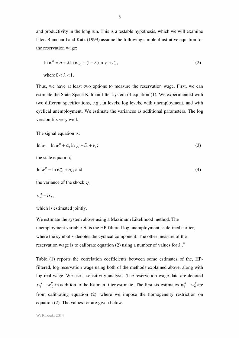
and productivity in the long run. This is a testable hypothesis, which we will examine
later. Blanchard and Katz (1999) assume the following simple illustrative equation for
the reservation wage:
ttt
R
t ywaw ln)1(lnln 1 , (2)
where 10 .
Thus, we have at least two options to measure the reservation wage. First, we can
estimate the State-Space Kalman filter system of equation (1). We experimented with
two different specifications, e.g., in levels, log levels, with unemployment, and with
cyclical unemployment. We estimate the variances as additional parameters. The log
version fits very well.
The signal equation is:
ttt
R
tt uyww ~lnlnln 1 ; (3)
the state equation;
t
R
t
R
t ww 1lnln ; and (4)
the variance of the shock t
2
2 ,
which is estimated jointly.
We estimate the system above using a Maximum Likelihood method. The
unemployment variable u~ is the HP-filtered log unemployment as defined earlier,
where the symbol denotes the cyclical component. The other measure of the
reservation wage is to calibrate equation (2) using a number of values for .ii
Table (1) reports the correlation coefficients between some estimates of the, HP-
filtered, log reservation wage using both of the methods explained above, along with
log real wage. We use a sensitivity analysis. The reservation wage data are denoted
RRww 101 in addition to the Kalman filter estimate. The first six estimates RR
ww 61 are
from calibrating equation (2), where we impose the homogeneity restriction on
equation (2). The values for are given below.

6
W. Razzak, 2014
Parameter values used to calibrate ttt
R
t ywaw ln)1(lnln 1 -
Homogeneity restriction imposed R
w1 ]50.0,65.2[ a
Rw2 ]75.0,65.2[ a
Rw3 ]85.0,65.2[ a
Rw4 ]90.0,65.2[ a
Rw5 ]95.0,65.2[ a
Rw6 ]99.0,65.2[ a
Parameter values used to calibrate tt
R
t ywaw lnlnln 211 - Homogeneity
restriction not imposed so the weights on lagged wages and productivity do not sum
up to one R
w7 ]15.0,90.0,65.2[ 21 a
Rw8 ]10.0,95.0,65.2[ 21 a
Rw9 ]25.0,95.0,65.2[ 21 a
Rw10 ]10.0,99.0,65.2[ 21 a
Finally, we have the reservation wage estimated using the Kalman filter and the real
wage. Table (1) shows that these measures are highly correlated over the business
cycle regardless of whether the homogeneity restriction is imposed, or not. However,
a small value of , e.g., 0.50, which means a larger weight on productivity, produces
a reservation wage estimate that is less correlated with the other estimates. Essentially,
the reservation wage is dependent more on lagged wages than on productivity. It
suggests that the value of is not necessarily equal to one as in Shapiro and Stiglitz
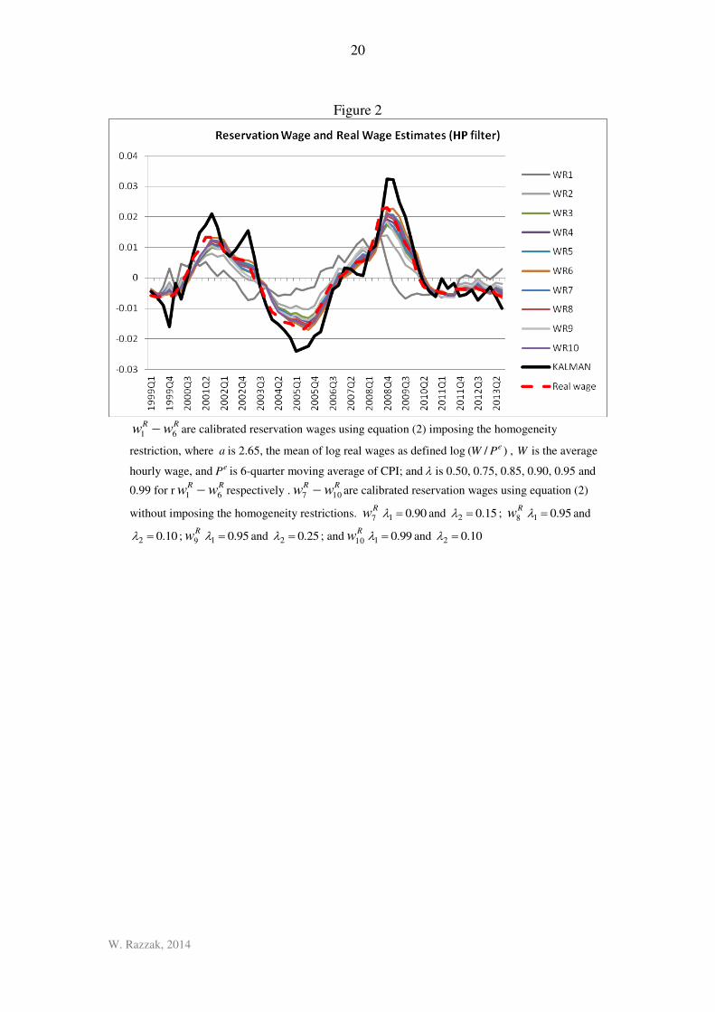
(1984) and to Blanchard and Katz (1999). Figure (2) plots all the estimates along with
the real wage (HP-filtered).
Given our estimates of the real wage and the reservation wage, we calculate the wage
gap (the log real wage – log reservation wage), but we drop the extreme estimates,
which correspond to the reservation wages with low value of , i.e., 50.0
and 75.0 . We have wage gaps corresponding to the estimated reservation wages,

7
W. Razzak, 2014
and the Kalman filter. We plot the data in figure (3). The estimates are highly
correlated.
The theory predicts that the covariance between the wage gap and unemployment is
negative because when the real wage is greater than the reservation wage the worker
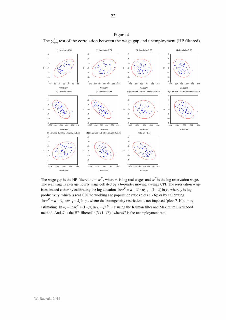
takes the job, hence unemployment falls. We test the covariance for each estimate of
the wage gap and the unemployment rate. We test the correlations using a confidence
ellipse, which is distributed 2
95.0,1 . Figure (4) plot the confidence ellipses. Some
correlations are positive, which are inconsistent with the theory. These are found in
plots 1, 2, 3, which correspond to wage gaps, where the reservation wage are
calibrated using equation (2), and the weight , is either low (0.50, 0.75 and 0.85) or
the homogeneity restriction is not imposed and the weight on productivity is > 0.10.
There are two cases, where the correlation is positive; these are plots 7 and 9, which
correspond to Rw7 and R
w9 , where 90.01 and 15.02 and 95.01 and
25.02 for Rw7 and R
w9 respectively. Generally, the test suggests that for the
prediction of the theory to hold (i.e. the gap between the real wage and the reservation
wage and unemployment are negatively correlated), the homogeneity restriction need
not be imposed, but the weight on productivity in equation (2) should still be smaller
than the weight on lagged waged. In other words, productivity affects the reservation
wage and the real wage, but the effect is smaller than the effect of lagged wages.
Table (2) reports a number of regressions using the wage gaps that are, statistically
significantly, negatively correlated with unemployment in figure (4). The wage gap,
depending on measurement, can explain up to 50 percent of unemployment’s
fluctuations over the business cycle.
3. The firm’s decision
The firm’s decision to hire workers has not been empirically tested in macroeconomic
models of unemployment. Over the business cycle, the firm hires workers as long as
the marginal product of labor exceeds the real wage; it stops hiring additional workers
when the marginal product of labor is equal to the real wage; and it lays-off workers
when the marginal product is lower than the real wage. The marginal product of labor
can deviate from the real wage over the business cycle, and for a number of reasons.

8
W. Razzak, 2014
Thurow (1968) provides some insight. The wedge exists because: (1) Taxes can create
a wedge if the incidence of the indirect taxes is on labor. (2) Monopoly power can
explain differences between the marginal product of factor inputs and their prices. (3)
Constant substitution between factor inputs along growth path could create a wedge
between the real wage and the marginal product of labor. As the stock of capital rises,
labor is displaced. Given output, less labor input causes its marginal productivity to be
higher than its rate of return, i.e. real wages. This wedge can persist if the transition
cost along the growth path is high. (4) Firms set the wage rate by the marginal product
of the marginal worker rather than the marginal product of the average worker, due to
heterogeneity. Maré and Hyslop, (2006, 2008) provide evidence that less skilled labor
is hired at the up-turn of the New Zealand business cycle. If this were the case, then
wages will have to be lower than the marginal product of the average worker. (5) Risk
premiums create a wedge between the marginal product of labor and the real wage. (6)
When social returns are not equal to private returns, actual returns must be corrected
for taxes when possible. (7) Endogenous growth models assume an increasing return
to scale rather (i.e., less than doubling factor inputs is needed to double output), which
means that capital and labor will more than exhaust total output.
The covariance between the wedge (real wages minus the marginal product of labor)
and the unemployment rate over the business cycle is positive. Unemployment
increases when the wedge is > 0 because the firm lays-off workers.
Computing the wedge requires an estimate of the marginal product of labor. We
assume a simple representative agent, where production is given by the Cobb –
Douglas production function. The first-order condition would equation the marginal
product of labor to the real wage.
Let the production function be a constant return to scale Cobb – Douglas:
LAKY 1 , (5)
Where Y is real GDP, K is the stock of capital and L is labor, which is measured
either in hours-worked or working age population. The parameter is the share of
labor.
The marginal product of labor is:

9
W. Razzak, 2014
,/11hYLAKmpl
h
Y (6)
which we can calibrate given K , L , and .
The stock of capital is measured using data on fixed capital formation, and an
assumed value of the initial stock of capital and the depreciation rate. We assume that
the stock of capital in the U.S. is approximately three times as big as GDP (e.g.,
Obstfeld and Rogoff, 1996) and the depreciation rate is somewhere between 5 and 8
percent annually. For labor, we use the working age population (15-64).
There are issues about measuring the share of labor, Krueger (1999). Karabarbunis
(2014) provides four measures, and reports the correlation coefficients. First is BEA
unadjusted, which is total compensation to employee / national income.iii
Second is
BEA adjusted, where he treats compensations to employee as unambiguous labor
income, proprietor’s income and net taxes on production and imports as ambiguous
income, and all other categories such as rental income, corporate profits, and business
transfers as unambiguous capital income. Third is BLS corporate, which does not
require imputations of the labor earnings of sole proprietors, he uses labor share for
the corporate sector. It is the ratio of corporate compensations to employee / gross
value added of the corporate sector.iv
Fourth is BEA corporate, which is the share in
the non-financial sector. These measures are highly, statistically significantly,
correlated. Table (3) reports the correlation matrix. Figure (5) plots our estimates of
the share of labor as in BEA above, which turns out to be sufficient for our purpose. It
has been declining over time. To calibrate the marginal product of labor we use our
estimates of the stock of capital, working age population and the share of labor.
Gali (2005) argued that the time series properties of hours worked and employment or
working age population can give rise to differences in measurements. To check the
robustness of our estimate we calibrate the marginal product of labor using hours
worked and working age population separately. Figure (6) plots both estimates.
We report the correlations between various measures of the wedge in table (4). They
differ in the way the real wage is computed. Figure (7) plots the four measures. Figure

10
W. Razzak, 2014
(8) plot the different measures of the wedge with unemployment. The correlation is
significant and positive as predicted by the theory.
We summarize the effects of the wage gap and the wedge on unemployment using an
unrestricted VAR.
,2211 tptpttt XXXcX (7)
where, X is an )1( n vector containing three variables, which are the HP-filtered
measures of the wage gap, the wedge and unemployment. The wage gap is our
measure of the difference the real wage and the reservation wage. The real wage
is ePWw / . We use the Kalman filter’s measure of the reservation wage (see figure
4). The wedge is the real wage minus the marginal product of labor, which we
presented earlier. The error term is also a vector t , which is distributed i.i.d. ),0( N
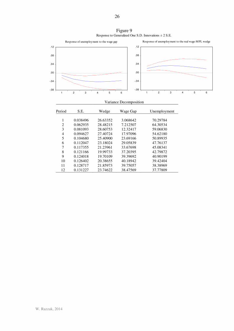
Figure (9) plots the VAR’s generalized impulse response functions of unemployment
to the innovations of the wage gap and to the wedge. Ordering of the variables in the
VAR is no longer a problem since the generalized impulse response function since
Pesaran and Shin (1998) describe the impulse response function, where they construct
an orthogonal set of innovations that does not depend on the VAR ordering. We use a
Monte-Carlo with 10000 iterations to estimate the standard errors. The wage gap
shock decreases unemployment and the wedge shock increases unemployment over
the business cycle. Variance decomposition shows the growing importance of the
wage gap and the wedge between the real wage and the marginal product of labor on
unemployment. From period 6 to 12, they explain more than 50 percent of the
variance of unemployment.
Earlier we showed that the wage gap explains about 30 – 50 percent of the
fluctuations in unemployment over the business cycle. Table (5) reports some
regression results to show that the wedge and the change in the wedge can explain an
additional 40 percent of the fluctuations in unemployment. The two variables, the
wage gap and the wedge, explain nearly 80 percent of unemployment. Most of the
remaining unexplained variation is the dynamic, which is attributed to smoothing the
data by the HP filter (Razzak, 1997)

11
W. Razzak, 2014
4. Conclusion
The empirical record of modern unemployment theories and models such as the
efficiency wage theory, e.g., Shapiro and Stiglitz (1984) Shirking model and the
dynamic search and matching of Mortensen and Pissarides (1994) is weak. Dynamic
search and matching models of unemployment predict that the volatility of the
employment – vacancy ratio and average labor productivity are the same while the
U.S. data show that the standard deviation of the unemployment-vacancy ratio is 20
times larger than that of average labor productivity, Shimer (2005).
Unemployment theories and models account for the wage gap, which is the difference
between the real wage and the reservation wage only. In this setup, the increase in
unemployment reduces real wages given reservation wages and productivity. The
wage gap between the real wage and the reservation wage is best interpreted as the
decision the worker’s make when faced with a wage offer. The worker accepts the job
offer with a certain real wage when the real wage exceeds his or her reservation wage,
given productivity. There is, however, another microeconomic-level decision not
accounted for by most models of unemployment. It is the firm’s decision to hire labor.
Over the business cycle, firms hire workers as long as the real wage is lower than the
marginal productivity of labor; they stop hiring workers when the real wage is equal
to the marginal productivity of labor; and they lay off workers when the real wage
exceeds the marginal productivity of labor.
By modeling both microeconomic decisions, the macroeconomic data are consistent
with the micro decisions above. We use quarterly data from 1999 to 2013 for the U.S.
to measure the real wage, the reservation wage, and the wedge between real wage and
the marginal product of labor and show that these shocks have impulse response
functions as predicted by the microeconomic theory and their variances explain more
than 50 percent of the variation of unemployment. We also show that while the wage
gap explains up to 50 percent of the unemployment dynamic, the wedge between the
real wage and the marginal product of labor can explain an additional 30 percent of
12
W. Razzak, 2014
unemployment dynamics. The remaining unexplained dynamic of unemployment is a
statistical artifact related to the use of smoothing.

13
W. Razzak, 2014
References
Barro, R. J. Unanticipated Money Growth and Unemployment in the United States,
American Economic Review, 67, 1977, 101-15.
Baxter, M. and R. King. Measuring Business Cycles Approximate Band-Pass
Filters For Economic Time Series. Review of Economics and Statistics 81(4), 1999,
575-593.
Blanchard, O. and L. Katz. Wage Dynamics: Reconciling Theory and Evidence.
American Economic Review 89 (3), 1999, 69-74.
Christaino, L. J. and Fitzgerald. The Band Pass Filter, International Economic
Review, Vol.44, Issue 2, 435-465.
Daly, C. B. Hobijn, A. Sahin and R. Valletta. A Search and Matching Approach to
Labor Markets: Did the Natural Rate of Unemployment Rise? Journal of Economic
Perspectives, 26(3), Summer 2012, 3-26.
Gali, J. Trends in Hours, Balanced Growth and the Role of Technology in the
Business Cycle. NBER, WP No. 11130, 2005.
Karabarbounis, L. The Labor Wedge: MRS vs. MPN. Review of Economic Dynamic,
17, 2014, 206-223.
Karabarbounis, L. and B. Neiman. The Global Decline of the Labor Share. NBER
WP No. 19136, 2013.
Maré, D. C., and D. R. Hyslop. Cyclical Earnings Variation and the Composition of
Employment. Statistics New Zealand, 2008.
Maré, D. C., and D. R. Hyslop. Worker-Firm Heterogeneity and Matching: An
analysis using worker and firm fixed effects estimated from LEED. Statistics New
Zealand, LEED research report, 2006.
Mortensen, D. and C. Pissarides. Job Creation and Job Destruction in the Theory of
Unemployment. The Review of Economic Studies, Vol. 61, No. 3. July 1994, 397-
415
Obstfeld, M. and K. Rogoff. Foundation of International Macroeconomics. MIT Press,
1996.
Pesaran, M. Hashem and Yongcheol Shin. Impulse Response Analysis in Linear
Multivariate Models. Economics Letters, 58, 1998, 17-29.
Razzak, W. A. The Hodrick-Prescott Technique: A Smoother versus a Filter: An
Application to New Zealand GDP. Economics Letters 57, issue 2, 1997, 163-168.

14
W. Razzak, 2014
Shapiro, M. and J. Stiglitz. Equilibrium Unemployment as a Discipline Device.
American Economic Review 74, June 1984, 433-444.
Shimer, R. The Cyclical Behaviour of Equilibrium Unemployment and Vacancies,
American Economic Review, 2005, 25-49.
Thurow, L. C. Disequilibrium and Marginal Productivity of Capital and Labor.
Review of Economics and Statistics Vol. 50, No.1, 1968, 23-31.

15
W. Razzak, 2014
Table 1: Reservation Wage Correlations (HP-filtered)
R
w1 R
w2 R
w3 Rw4
Rw5
Rw6
Rw7
Rw8
Rw9
Rw10
Kalman reservation
wage R
w1 1.000000 R
w2 0.650233 1.000000 R
w3 0.460663 0.973860 1.000000 R
w4 0.382314 0.950613 0.996266 1.000000 R
w5 0.315967 0.926062 0.987421 0.997245 1.000000 R
w6 0.269057 0.906512 0.978607 0.992632 0.998792 1.000000 R
w7 0.450089 0.970710 0.999482 0.996755 0.989409 0.981082 1.000000 R
w8 0.376595 0.948400 0.995391 0.999645 0.997904 0.993519 0.996729 1.000000 R
w9 0.566496 0.994425 0.992383 0.978042 0.960621 0.945926 0.990434 0.976435 1.000000
Rw10 0.371603 0.946690 0.994886 0.999605 0.998238 0.994117 0.996278 0.999985 0.975274 1.000000
Kalman 0.232124 0.862254 0.937944 0.953891 0.962094 0.964621 0.941003 0.955216 0.903047 0.955942 1.000000 Reservation
Wage 0.456463 0.955083 0.979319 0.975144 0.966935 0.957911 0.979904 0.975256 0.972599 0.974719 0.959104 1.000000
RR
ww 61 are calibrated reservation wages using equation (2) imposing the homogeneity restriction, where a is 2.65, the mean of log real wages as defined log )/( ePW ,
W is the average hourly wage, and eP is 6-quarter moving average of CPI; and is 0.50, 0.75, 0.85, 0.90, 0.95 and 0.99 for WR1 to WR6. For WR7-WR10 are calibrated
reservation wages using equation (2) without imposing the homogeneity restrictions.R
w7 90.01 and 15.02 ;R
w8 95.01 and 10.02 ; R
w9 95.01 and
25.02 andR
w10 99.01 and 10.02

16
W. Razzak, 2014
Table 2
Dependent variable )1/ln(~ UUu (i)
(1999Q2 – 2013Q3)
Coefficient Estimates (P values)
5gapwage (ii) -0.36
(0.0000)
- - -
6gapwage (ii) - -0.41
(0.0000)
- -
8gapwage (iii) - - -0.26
(0.0001)
-
)(Kalmangapwage (iv) - - - -0.16
(0.0001) 2
R 0.34 0.53 0.15 0.25
0.0012 0.0010 0.0014 0.0013
(i) u~ is the HP filtered series of )1/ln( UU , whereU is the unemployment rate.
(ii) Wage gaps are HP filtered Rww lnln , where w is real wages and
Rw is the reservation wage. The
real wage is average hourly wage deflated by a 6-quarter moving average CPI. In wage gaps 5 and
6,R
w is calibrated using ywaw tR ln)1(lnln 1 , where a is the mean log real wage equal
to 2.65, y is productivity measured as GDP/working age population ratio, and is 0.95 and 0.99
respectively.
(iii) In wage gap 8, Rw is calibrated using ywaw t
R lnlnln 211 , where 95.01 and 10.02
so that the homogeneity restriction is not imposed.
(iv) The wage gap based on the Kalman filter’s estimates of the reservation wage.
(v) P values are in parentheses.
(vi) Standard errors and covariance matrix are estimated by the Newey-West method with Bartlett
Kernel bandwidth = 4).

17
W. Razzak, 2014
Table 3
The Correlation Matrix of Measures of the Labor Shares
(HP filtered)
BEA unadjusteBEA adjusted BLS corporate BEA corporate
BEA unadjusted 1.00
BEA adjusted 0.96 1.00
BLS corporate 0.85 0.86 1.00
BEA corporate 0.86 0.87 0.95 1.00
Source (Karabarbunis , 2014)
Table 4
The Correlation Matrix of Measures of the Wedge
(HP filtered)
Wedge 1 Wedge 2 Wedge 3 Wedge 4
Wedge 1 1.00
Wedge 2 0.98 1.00
Wedge 3 0.97 0.98 1.00
Wedge 4 0.98 0.97 0.96 1.00 Wedge is the real wage minus the marginal product of labor.
The marginal product of labor is 160.04.06.0 LK , where L is working age population.
Wedge1, 2, 3, and 4 differ in how the real wage is measured only.
Wedge 1:real wage is the nominal wage adjusted for expected inflation measure as a 6-quarter moving
average of annual CPI inflation.
Wedge 2: real wage is the nominal wage adjusted for expected inflation measured by the Philadelphia
fed survey measure.
Wedge3: real wage is the nominal wage adjusted for expected inflation measured by the University of
Michigan survey measure.
Wedge4: real wage is the nominal wage deflated by a 6-quarter moving average of the CPI level.

18
W. Razzak, 2014
Table 5
Regressions: Dependent variable )1/ln(~ UUu (i)
Coefficients
Wage gap 5 (ii) -02.0
(0.0007)
-- -- --
Wage gap 6 (ii) -- -0.24
(0.0000)
-- --
Wage gap 8 (iii) -- -- -0.15
(0.0118)
--
Wage gap (Kalman) (iv) -- -- -- -0.18
(0.0043)
Wedge (v) 0.20
(0.0005)
0.17
(0.0009)
0.23
(0.0001)
0.23
(0.0001)
Wedge 0.51
(0.0000)
0.43
(0.0000)
0.55
(0.0000)
0.53
(0.0000)
2R 0.73 0.78 0.69 0.70
0.0008 0.0007 0.0008 0.0008
(i) u~ is the HP filtered series of )1/ln( UU , whereU is the unemployment rate.
(ii) Wage gaps are HP filtered Rww lnln , where w is real wages and
Rw is the reservation
wage. The real wage is average hourly wage deflated by a 6-quarter moving average CPI.
In wage gaps 5 and 6,R
w is calibrated using ywaw tR ln)1(lnln 1 , where a is
the mean log real wage equal to 2.65, y is the natural log of productivity measured as
GDP/working age population ratio, and is 0.95 and 0.99 respectively.
(iii) In wage gap 8, Rw is calibrated using ywaw t
R lnlnln 211 , where 95.01 and
10.02 so that the homogeneity restriction is not imposed.
(iv) The wage gap based on the Kalman filter’s estimate of the reservation wage.
(v) Wedge: real wage is the nominal wage deflated by a 6-quarter moving average of the
CPI level.
(vi) Both, the dependent variable and the independent variable in the equation above are
deviations from the HP filter.
(vii) P values are in parentheses.
(viii) Standard errors and covariance matrix are estimated by the Newey-West method with
Bartlett Kernel bandwidth = 4).

19
W. Razzak, 2014
Figure 1
-0.03
-0.02
-0.01
0
0.01
0.02
0.03
0.041999Q1
1999Q3
2000Q1
2000Q3
2001Q1
2001Q3
2002Q1
2002Q3
2003Q1
2003Q3
2004Q1
2004Q3
2005Q1
2005Q3
2006Q1
2006Q3
2007Q1
2007Q3
2008Q1
2008Q3
2009Q1
2009Q3
2010Q1
2010Q3
2011Q1
2011Q3
2012Q1
2012Q3
2013Q1
2013Q3
Real Wages (HP filter)
w1
w2
w3
w4
31 ww are average hourly wage adjusted for expected inflation measures as
6-quarter moving average of CPI inflation, the Philadelphia fed’s survey of inflation expectations
and the Michigan University’s survey of inflation expectations respectively. 4w is log )/( ePW ,
W is the average hourly wage, and eP is 6-quarter moving average of CPI.
20
W. Razzak, 2014
Figure 2
RR
ww 61 are calibrated reservation wages using equation (2) imposing the homogeneity
restriction, where a is 2.65, the mean of log real wages as defined log )/( ePW , W is the average
hourly wage, and eP is 6-quarter moving average of CPI; and is 0.50, 0.75, 0.85, 0.90, 0.95 and
0.99 for rRR
ww 61 respectively .RR
ww 107 are calibrated reservation wages using equation (2)
without imposing the homogeneity restrictions. R
w7 90.01 and 15.02 ; R
w8 95.01 and
10.02 ;R
w9 95.01 and 25.02 ; andR
w10 99.01 and 10.02

21
W. Razzak, 2014
Figure 3
22
W. Razzak, 2014
Figure 4
The 2
95.0 test of the correlation between the wage gap and unemployment (HP filtered)
-.6
-.4
-.2
.0
.2
.4
.6
-.03 -.02 -.01 .00 .01 .02 .03
WAGEGAP
U
(1) Lambda=0.50
-.6
-.4
-.2
.0
.2
.4
.6
-.012 -.008 -.004 .000 .004 .008 .012
WAGEGAP
U
(2) Lambda=0.75
-.6
-.4
-.2
.0
.2
.4
.6
-.008 -.004 .000 .004 .008 .012
WAGEGAP
U
(3) Lambda=0.85
-.6
-.4
-.2
.0
.2
.4
.6
-.008 -.004 .000 .004 .008 .012
WAGEGAP
U
(4) Lambda=0.90
-.6
-.4
-.2
.0
.2
.4
.6
-.008 -.004 .000 .004 .008 .012
WAGEGAP
U
(5) Lambda=0.95
-.6
-.4
-.2
.0
.2
.4
.6
-.008 -.004 .000 .004 .008 .012
WAGEGAP
U
(6) Lambda=0.99
-.6
-.4
-.2
.0
.2
.4
.6
-.008 -.004 .000 .004 .008
WAGEGAP
U
(7) Lambda 1=0.90; Lambda 2=0.15
-.6
-.4
-.2
.0
.2
.4
.6
-.008 -.004 .000 .004 .008
WAGEGAP
U
(8) Lambda 1=0.95; Lambda 2=0.10
-.6
-.4
-.2
.0
.2
.4
.6
-.008 -.004 .000 .004 .008
WAGEGAP
U
(9) Lambda 1= 0.95; Lambda 2=0.25
-.6
-.4
-.2
.0
.2
.4
.6
-.008 -.004 .000 .004 .008
WAGEGAP
U
(10) Lambda 1= 0.99; Lambda 2=0.10
-.6
-.4
-.2
.0
.2
.4
.6
-.015 -.010 -.005 .000 .005 .010 .015
WAGEGAP
U
Kalman Filter
The wage gap is the HP-filteredR
ww , where w is log real wages andR
w is the log reservation wage.
The real wage is average hourly wage deflated by a 6-quarter moving average CPI. The reservation wage
is estimated either by calibrating the log equation ywaw tR ln)1(lnln 1 , where y is log
productivity, which is real GDP to working age population ratio (plots 1 - 6); or by calibrating
ywaw tR lnlnln 211 , where the homogeneity restriction is not imposed (plots 7-10); or by
estimating tttRtt uyww ~ln)1(lnln using the Kalman filter and Maximum Likelihood
method. And, u~ is the HP-filtered )1/ln( UU , whereU is the unemployment rate.

23
W. Razzak, 2014
Figure 5
The Share of Labor

24
W. Razzak, 2014
Figure 6
Marginal Product of Labor

25
W. Razzak, 2014
Figure 7
Measures of the Wedge
Figure 8
Measures of the Wedge and Unemployment
26
W. Razzak, 2014
Figure 9
-.08
-.04
.00
.04
.08
.12
1 2 3 4 5 6
Response of unemployment to the wage gap
-.08
-.04
.00
.04
.08
.12
1 2 3 4 5 6
Response of unemployment to the real wage-MPL wedge
Response to Generalized One S.D. Innovations ± 2 S.E.
Variance Decomposition
Period S.E. Wedge Wage Gap Unemployment
1 0.038496 26.63352 3.068642 70.29784
2 0.062935 28.48215 7.212507 64.30534
3 0.081093 28.60753 12.32417 59.06830
4 0.094627 27.40724 17.97096 54.62180
5 0.104680 25.40900 23.69166 50.89935
6 0.112047 23.18024 29.05839 47.76137
7 0.117355 21.23961 33.67698 45.08341
8 0.121166 19.99733 37.20395 42.79872
9 0.124018 19.70109 39.39692 40.90199
10 0.126402 20.38655 40.18942 39.42404
11 0.128717 21.85973 39.75057 38.38969
12 0.131227 23.74622 38.47569 37.77809

27
W. Razzak, 2014
Data Appendix
Variable Description and sources
U Seasonally adjusted civilian unemployment rate. Source: US Department of Labor.
Y Seasonally adjusted real chain GDP. Source: Department of Commerce, Bureau of
Economic Analysis.
P Seasonally adjusted CPI for all urban consumers, all items. Source: U.S. Department of
Labor Statistics.
W Seasonally adjusted average hourly earnings of production and nonsupervisory Employees:
Total Private. Source: U.S. Department of Labor: Bureau of Labor Statistics. e (1) Federal Reserve Bank of Philadelphia Survey of inflation expectations. (2) The
University of Michigan Survey of inflation expectations.
L Seasonally adjusted Working Age Population: Aged 15-64: All Persons for the United
States. Source: OECD; and, average weekly hours. It is the employment rate*total annual
hours worked / 52. Source: OECD.
Fixed
capital
formation
Gross Domestic Product by Expenditure in Constant Prices: Gross Fixed Capital
Formation for the United States. Source: OECD.
WAP Seasonally adjusted working age population: Aged 15-64: All Persons for the United
States. Source: OECD
i It does not really matter whether we measured the unemployment in log form or not. It is just more
convenient for interpreting the coefficients. In a log form we can interpret regression coefficients as
elasticity. For example, see Barro (1977).
ii The HP filter , the Band Pass filter (Baxter-King, 1997) or the Christiano-Fitzgerald (2005) produce
similar cyclical results, albeit the BP filter produces smoother cycles than the HP filter. iii
The data are line 1 and 2 of NIPA, table 1.12. iv The data are in line 4 of NIPA, Table 1.14.
Recommended