Wavelet analysis of intraday share prices
Pieter Stoffberg
83160150
A research project submitted to the Gordon Institute of Business
Science, University of Pretoria, in partial fulfilment of the
requirements for the degree of Master of Business Administration.
10 November 2014
© 2014 University of Pretoria. All rights reserved. The copyright in this work vests in the University of Pretoria.

i
Abstract
This research tested whether wavelet based algorithms can improve the
performance of intraday share trading algorithms. The trading algorithms
investigated, each consisted of two parts: the first part performed share price
prediction and the second part traded based on the prediction.
All the trades in the shares BTI, MTN, NPN and SBK through 2013 on the JSE
with the associated time stamps, transaction share prices and volumes, served
as the basic sample. The sample was further reduced by using end-of-interval
transaction share prices at intervals of one, two, five and ten minutes
throughout the trade days.
Three types of prediction algorithms were employed: auto regressive moving
average (ARMA), wavelet-ARMA and wavelet regressive algorithms. The
wavelet based algorithms were further broken down by using up to six different
levels of scales in each of the algorithms. These algorithms were fitted using the
first half year of data while the tests were conducted on the second half year of
data.
Two trade algorithms were created by the researcher: One algorithm for buy-
and-sell and another for short-and-close. Both algorithms used the predicted
share price one and two intervals ahead as input and took transaction cost into
account. The trade algorithms entered the market daily after opening time and
exited the market before closing time.
The wavelet based algorithms were not found to improve the accuracy of share
price prediction. However, in agreement with previous research, wavelet based
algorithms were found to improve the accuracy of predicting the direction of the
share prices. The wavelet based algorithms were also found to improve trading
performance. Short-and-close algorithms outperformed buy-and-sell. None of
the intraday trade algorithms were found to outperform buy-and-hold over the
test period.
© 2014 University of Pretoria. All rights reserved. The copyright in this work vests in the University of Pretoria.

ii
This study contributes to academic research regarding the manner in which
wavelet based and ARMA algorithms were combined, the application of a
wavelet-regressive prediction method to financial time series and the application
of wavelet based trading algorithms on an intraday time scale.
© 2014 University of Pretoria. All rights reserved. The copyright in this work vests in the University of Pretoria.

iii
Keywords
Algorithmic trading; ARMA; Intraday; Wavelet.
© 2014 University of Pretoria. All rights reserved. The copyright in this work vests in the University of Pretoria.

iv
Declaration I declare that this research project is my own work. It is submitted in partial
fulfilment of the requirements for the degree of Master of Business
Administration at the Gordon Institute of Business Science, University of
Pretoria. It has not been submitted before for any degree or examination at any
other University. I further declare that I have obtained the necessary
authorisation and consent to carry out this research.
______________ 10 November 2014
Pieter Stoffberg Date
© 2014 University of Pretoria. All rights reserved. The copyright in this work vests in the University of Pretoria.

v
Acknowledgements I am using this opportunity to express my gratitude to the following people for
the part each one played in assisting me in completing this research project:
My supervisor, Chris Muller, for his patience, insights, guidance and
encouragement throughout the process.
Prof. Dawie de Jongh at the Centre of Business Mathematics and Informatics of
the North West University, for extracting and sharing the data.
Suhagna Mansura at the JSE, for explaining the JSE cost structure.
Thea Bruwer and my father, Pierre Stoffberg, for proof reading the draft thesis
and giving me valuable input.
My daughter, Maret, for assisting with the data reduction.
My spouse and children, Karin, Pierre, Maret, Arend and Eduard, for their
encouragement and patience during the last two years.
© 2014 University of Pretoria. All rights reserved. The copyright in this work vests in the University of Pretoria.

vi
List of tables
Table 1. Sampling intervals and the number of trade data points .................... 19
Table 2. Scales and the sampling intervals ...................................................... 22
Table 3. Marginal JSE trade cost for a broker .................................................. 26
Table 4. Shares, time steps, prediction methods and error measurements ..... 27
Table 5. Shares, time steps, prediction methods and trading algorithms ......... 28
Table 6. Descriptive statistics through period ................................................... 32
Table 7. Descriptive statistics per day .............................................................. 32
Table 8. Number of data points used for fitting prediction algorithms ............... 33
Table 9. Rank of algorithms with lowest prediction error .................................. 35
Table 10. Rank of algorithms performing best in predicting the direction of price changes of the next two time steps .................................................................. 36
Table 11. Descriptive statistics per sampling time interval ............................... 54
Table 12. ARMA models fitted to log returns .................................................... 55
Table 13. Wavelet-ARMA models fitted to BTI and MTN log returns ............... 56
Table 14. Wavelet-ARMA models fitted to NPN and SBK log returns .............. 58
Table 15. Wavelet regression coefficients fitted to log returns ......................... 60
Table 16. Wavelet algorithms with mean RMS prediction error for one and two time steps ahead smaller than ARMA .............................................................. 61
Table 17. Wavelet algorithms predicting the price change direction of the next two steps better than ARMA............................................................................. 62
Table 18. Shares with predicting and trading methods better than ARMA, buy-and-sell at time steps 1,2,5 and 10 minutes ..................................................... 68
Table 19. Algorithms and trade methods with positive cumulative returns ....... 69
© 2014 University of Pretoria. All rights reserved. The copyright in this work vests in the University of Pretoria.

vii
List of figures
Figure 1. Sample wavelet functions: Haar (left) and Morlet (right). .................... 9
Figure 2. Cumulative log returns of share prices through trade days of 2013. . 31
Figure 3. SKB log return and decomposed wavelet components ..................... 70
Figure 4. SKB log return and decomposed wavelet components – 12 days .... 71
Figure 5. SKB log return and decomposed wavelet components – 2 days ...... 72
Figure 6. BTI best trade algorithms .................................................................. 73
Figure 7. MTN best trade algorithms (short & close) ........................................ 74
Figure 8. NPN best trade algorithms (short & close) ........................................ 75
Figure 9. SBK best trade algorithms (short & close) ........................................ 76
Figure 10. Number of trades through the test period ........................................ 77
© 2014 University of Pretoria. All rights reserved. The copyright in this work vests in the University of Pretoria.

viii
List of abbreviations
AR Autoregressive
ARMA Autoregressive moving average
ARIMA Autoregressive integrated moving average
BIC Bayesian information criterion
BTI British American Tobacco PLC - JSE share code
DJIA Dow Jones Industrial Average
JSE JSE Limited (Johannesburg Stock Exchange)
MA Moving average
MODWT Maximum overlap discrete wavelet transform
MTN MTN Group – JSE share code
NPN Naspers Limited – JSE share code
RMS Root mean square
SBK Standard Bank Group Limited - JSE share code
© 2014 University of Pretoria. All rights reserved. The copyright in this work vests in the University of Pretoria.
ix
Contents Abstract…………………………………………………………………………………i
Keywords…………………………………………………………….……………......iii
Declaration…………………………………………………………….………………iv
Acknowledgements……………………………………………………..………….....v
List of tables………………………………………………………………..……….…vi
List of figures………………………………………………………………...………..vii
List of abbreviations……...………………………………………………………….viii
Chapter one - Introduction to the research problem .................................... 1
Chapter two - Literature review ....................................................................... 3
2.1 Introduction ........................................................................................... 3 2.2 Technical trading and prediction ........................................................... 3 2.3 Intraday trade ........................................................................................ 5 2.4 Algorithmic share trading ...................................................................... 6 2.5 Rate of exchange as share market indicator ......................................... 8 2.6 Transaction cost .................................................................................... 8 2.7 Wavelet theory ...................................................................................... 8 2.8 Wavelet analysis of time series ........................................................... 10
2.8.1 Natural cycles .................................................................................. 10 2.8.2 Economic cycles .............................................................................. 11 2.8.3 Electricity prices ............................................................................... 11 2.8.4 Rates of exchange ........................................................................... 12 2.8.5 Share prices ..................................................................................... 12 2.8.6 Intraday share prices ....................................................................... 13
2.9 Measures of algorithmic success ........................................................ 13 2.10 Conclusion of literature review ............................................................ 14
Chapter three - Research hypotheses .......................................................... 15
3.1 Hypothesis A ....................................................................................... 15 3.2 Hypothesis B ....................................................................................... 15 3.3 Hypothesis C ....................................................................................... 16 3.4 Hypothesis D ....................................................................................... 16
Chapter four - Research methodology ......................................................... 17
4.1 Introduction ......................................................................................... 17 4.2 Research philosophy........................................................................... 17 4.3 Unit of analysis .................................................................................... 17 4.4 Data source ......................................................................................... 18 4.5 Data preparation ................................................................................. 18 4.6 Sampling ............................................................................................. 18 4.7 Data splitting ....................................................................................... 19 4.8 Models for price prediction .................................................................. 20
4.8.1 ARMA .............................................................................................. 20 4.8.2 Wavelet-ARMA ................................................................................ 21
© 2014 University of Pretoria. All rights reserved. The copyright in this work vests in the University of Pretoria.

x
4.8.3 Wavelet regression .......................................................................... 23 4.9 Trading algorithm ................................................................................ 24
4.9.1 Buy-and-sell ..................................................................................... 24 4.9.2 Short-and-close ............................................................................... 25 4.9.3 Trading cost ..................................................................................... 25
4.10 Comparisons ....................................................................................... 27 4.10.1 Accuracy of price prediction ......................................................... 27 4.10.2 Performance of trade algorithms .................................................. 27
4.11 Exclusions ........................................................................................... 28 4.12 Research limitations ............................................................................ 28
Chapter five – Results ................................................................................... 30
5.1 Introduction ......................................................................................... 30 5.2 Description of the sample share price data ......................................... 30 5.3 Prediction algorithms........................................................................... 33
5.3.1 ARMA .............................................................................................. 33 5.3.2 Wavelet-ARMA ................................................................................ 33 5.3.3 Wavelet regression .......................................................................... 34
5.4 Prediction accuracy ............................................................................. 34 5.4.1 Prediction of share price accuracy ................................................... 35 5.4.2 Prediction of direction accuracy ....................................................... 36
5.5 Trading performance ........................................................................... 36 5.6 Intraday trading algorithms vs. buy-and-hold ...................................... 38 5.7 Trading cost and number of transactions ............................................ 38 5.8 Conclusion of the results chapter ........................................................ 38
Chapter six - Discussion of results .............................................................. 40
6.1 Introduction ......................................................................................... 40 6.2 Algorithm fit ......................................................................................... 40 6.3 Accuracy of price prediction ................................................................ 40 6.4 Accuracy of direction prediction .......................................................... 41 6.5 Trade algorithm performance .............................................................. 42 6.6 Buy and hold ....................................................................................... 43 6.7 The effect of trading cost ..................................................................... 43 6.8 Conclusion regarding the results ......................................................... 43
Chapter seven – Conclusion ......................................................................... 44
7.1 Introduction ......................................................................................... 44 7.2 Main findings ....................................................................................... 44 7.3 Recommendations to industry ............................................................. 45 7.4 Suggestions for future research .......................................................... 46 7.5 Concluding remarks ............................................................................ 47
References ...................................................................................................... 48
Appendix A: Tables with result details ........................................................ 54
Appendix B: Graphs with result details ....................................................... 70
© 2014 University of Pretoria. All rights reserved. The copyright in this work vests in the University of Pretoria.

1
Chapter one - Introduction to the research problem
The future path of the price level of a security is no more predictable than the
path of a series of cumulated random numbers – Eugene Fama.
Share trading is increasingly done by computer algorithms without direct human
intervention (Menkveld, 2013). Profitable trading (in contrast with investing)
increasingly occurs intraday, rather than at longer periods (Schulmeister, 2009).
High frequency trading occurs at response times of milliseconds and accounts
for half of the transactions in the USA (Mackenzie, 2014; Aitken, Cumming &
Zhan, 2014).
Trading algorithms can incorporate models of the order book dynamics and of
share price movement (Mackenzie, 2014). Such models can include the effects
of external factors (for instance macro-economic variables and the price
movement of other assets) and own price history effects (such as momentum)
(Zheng & Chen, 2012).
Share price time histories contain cycles with varying periods and amplitudes.
The cycles are treated as short term bull or bear markets in some investment
strategies. For instance, if momentum is used as an investment style, the cycles
are viewed either as trends within the time period considered (momentum up or
down) (Schulmeister, 2009) or, in the case of shorter cycles, noise. A
complementary approach is to use the cycles as features when modelling and
predicting price movement (Kriechbaumer, Angus, Parsons & Rivas Casado,
2014).
Wavelet analysis is useful to decompose financial (and other) time series to
reveal the cyclic nature (or frequency response) of the time series and how the
frequency response changes over time (Bekiros & Marcellino, 2013). It can also
be used to investigate links between assets at different time scales (Jammazi,
2012).
No trading algorithms have been found reported that use wavelets as part of the
algorithm in intraday trading. This research focused on intraday price prediction
© 2014 University of Pretoria. All rights reserved. The copyright in this work vests in the University of Pretoria.

2
algorithms and how wavelets could improve the algorithm performances for
signalling buy/sell in trading algorithms.
© 2014 University of Pretoria. All rights reserved. The copyright in this work vests in the University of Pretoria.

3
Chapter two - Literature review
Forecasting prices of stocks, commodities or derivatives on liquid markets is in
a large part guesswork – Stephan Schütler and Carola Deuschle.
2.1 Introduction
Returns from the stock market can be earned by investing or by trading.
Investing focuses on the intrinsic or fundamental value of companies with the
expectation that the value of a company’s shares plus dividends will grow due
to its performance (Schulmeister, 2009). Trading is more concerned with the
expected short term change in the share price and it is the focus of technical
analysis (Schulmeister, 2009). This study is about trading and the prediction of
share prices.
The literature review starts with an overview of issues related to technical
trading and prediction. Thereafter the subjects of intraday trade, algorithmic
trading and transaction cost are considered. Wavelet theory is introduced next
and thereafter a review of wavelet analysis of financial time series.
Measurement of algorithmic success is the last topic before the conclusion.
2.2 Technical trading and prediction
Schulmeister (2009) identified three groups of traders and their aggregate
response results in the market behaviour: Fundamentalists (value traders),
technical traders (relying mostly on recent price movements) and
“bandwagonists” (responding to trends). This study pertained to the technical
traders. Technical traders use rules based on patterns in asset prices and these
patterns occur due to human behaviour. (Friesen, Weller & Dunham 2009).
Technical trading’s mechanism for realising a return is prediction, therefore
good trading rules start with good prediction ability. However, it is not clear
whether technical analysis results in profitable trading, or in contrast, whether
one cannot consistently outperform the market (as the efficient market
hypothesis implies) (Duvinage, Mazza & Petitjean, 2013).
© 2014 University of Pretoria. All rights reserved. The copyright in this work vests in the University of Pretoria.
4
Various studies reported that technical trading could not outperform the market.
Hudson, Dempsey and Keasey (1996) applied two trading rules on the UK stock
market from 1935 to 1994 and found that their prediction ability is not sufficient
to make excess returns if trading fees are accounted for. Marshall, Cahan and
Cahan (2008) also reported that most studies find technical analysis is not
profitable if fees are taken into account. Du Plessis (2013) obtained the same
result with the FTSE/JSE Top 40 shares. An analysis of Japanese candlestick
strategies conducted at 5 minute intervals on the 30 stocks of DJIA over a year
concluded that buy-and-hold would be a better strategy (Duvinage et al., 2013).
Yamamoto (2012) compared trading strategies based on order flow imbalance
and order book imbalance of individual Nikkei 225 shares at 5 minute intervals
with buy-and-hold and came to the same conclusion. Marshall et al. (2008)
tested 7 846 popular technical trading rules on 2002-2003 US equity data at 5
minute intervals and found no intraday profits, even without accounting for
transaction costs.
In contrast, there are studies that claim technical trading can outperform the
market. Hudson et al., (1996) cited a study (Brock, W., Lakonishok, J., &
LeBaron, B. (1992). Simple technical trading rules and the stochastic properties
of stock returns. The Journal of Finance, 47(5), 1731-1764.) on the prediction
ability of simple trading rules with respect to the Dow Jones index from 1897 to
1992 with positive results. This outcome is supported by the reference to
various empirical studies conducted between 1986 and 2000 that report
evidence that technical analysis beats the market (Hong & Satchell, 2011).
Schulmeister (2009) found that the profitability of technical trading rules in the
S&P500 spot market declined over time from 8.6% per year in the 1960’s to as
low as -5.1% in the 1990’s and to -0.8% in the early 2000’s. However, technical
stock trading at 30 minute intervals showed a profit of 2.7% between the 1980’s
and early 2000’s. Schulmeister (2009) concluded that technical trading
profitability has shifted to intraday time scales.
© 2014 University of Pretoria. All rights reserved. The copyright in this work vests in the University of Pretoria.

5
2.3 Intraday trade
The daily volume of trade has increased significantly over time. On Black
Monday (the market crash day in October 1987), more than 6 million shares
were traded on the New York Stock Exchange. On the flash crash date (6 May
2010) 10.3 billion shares (1 700 times more, or 440 000 shares per second)
were traded (Betancourt, VanDenburgh & Harmelink, 2011). On average, five
billion shares were traded daily in the USA during 2013 (Mackenzie, 2014).
Daily trade activity tends to match a U shaped graph: High volumes of trade
occur at opening and closing times with the lowest activity recorded around
noon (Cont, 2011; Scholtus & Van Dijk, 2012). Cont, Kukanov and Stoikov
(2014) found high price volatility early in the trade day and high order flow
imbalance volatility by the end of the market day. The high price volatility in the
morning is ascribed to more information being available at that time (Cont et al.,
2014). There are also peaks in trade messages at regular intervals on the hour,
half hour, 5th, 15th and 45th minutes and every minute as well as at regular
intervals within the minute and within the second (Scholtus & Van Dijk, 2012).
These peaks are ascribed to market participants who trade at regular periods
(Scholtus & Van Dijk, 2012).
Heston, Korajczyk and Sadka (2010) analysed intraday trade on the New York
Stock Exchange and excluded trades adjacent to opening and closing times in
their analysis of intraday share price patterns. They selected 13 half-hour time
intervals per day and recorded the returns of shares over each interval. The
returns of shares were found to be negatively correlated with recent intervals.
However a positive correlation was found with every 13th interval (or every 24
hours). This daily correlation was statistically significant for 40 or more trading
days (Heston et al., 2010). Heston et al. (2010) considered the regular arrival of
news during the day as possibly contributing to the 24 hour correlation. Groß-
Klußmann and Hautsch (2011) investigated the high frequency effects of the
unannounced arrival of news items on share prices. They excluded the opening
and closing times of the market and the announcement of results. In contrast to
the deduction of Heston et al., (2010), no intraday news arrival pattern was
© 2014 University of Pretoria. All rights reserved. The copyright in this work vests in the University of Pretoria.
6
detected apart from an observation that more news arrived earlier in the day
(Groß-Klußmann & Hautsch 2011). Value, volatility, trade size and spread
increased before news arrival, then peaked with news arrival and later tapered
off. (Groß-Klußmann & Hautsch, 2011).
2.4 Algorithmic share trading
Modern stock exchanges use electronic order books. The process to conclude a
sale occurs by means of the exchange’s matching engine algorithm as soon as
bid and sell offer conditions match (Mackenzie, 2014). Mackenzie (2014)
identified three circumstances of trade:
1) Human actors, with the market consisting of humans interacting with
humans.
2) Human actors working via computers with the market being an algorithm.
3) An algorithmic market with mostly algorithmic actors directing trade.
One category of algorithmic trading is agency algorithms (Hasbrouck & Saar
2013). Agency algorithms are employed to buy or sell large blocks of shares at
the best possible average price. These algorithms would for instance divide the
shares in small quantities in order to hide the size of the trade (Mackenzie,
2014). Agency algorithms in general do not require millisecond response times
(Hasbrouck & Saar, 2013).
The other category of algorithmic trading is proprietary trading algorithms. With
proprietary trading algorithms, the intention is to buy-and-sell and not to
accumulate positions in shares (Mackenzie, 2014). Menkveld (2013), for
instance, found that a particular high frequency trader in general only realised
profits with positions being maintained for not longer than 5 seconds.
High frequency algorithms have low latency. Some of these algorithms trade
within 2 to 3 milliseconds after an event (Hasbrouck & Saar, 2013; Hagströmer
& Nordén, 2013). The time from posting a limit order to cancellation is on
average 0.36 milliseconds (Hagströmer & Nordén, 2013). Trade performance
declines significantly with delays exceeding 200 milliseconds, also in the case
of opportunistic trading (Scholtus & Van Dijk, 2012).
© 2014 University of Pretoria. All rights reserved. The copyright in this work vests in the University of Pretoria.
7
The order book, consisting of the offers to sell, bids to buy and the associated
volumes on offer/bid with the recent history, is the important input to the high
frequency algorithms (Cont et al., 2014; Treleaven, Galas & Lalchand, 2013).
Various strategies exist. If, for instance, the volume of the best bid price to buy
is larger than the volume of the best offer price to sell, the expectation is that
there is more buying force than selling force and the price is about to increase.
High frequency traders can exploit this by a practice called spoofing, by for
instance placing offers for very short periods to create an impression of supply,
and then removing the offers (Mackenzie, 2014).
High frequency trader strategies can be grouped as market making or market
taking. Market (or liquidity) makers position their offers and bids in the order
book as close as possible to the best bids to buy and best offers to sell. They
profit from the bid/offer price difference and earn on average about 0.08%
(Mackenzie, 2014). Market takers are participants who agree to the bid/offer
price and realise the sale.
Another group of algorithmic traders engage in opportunistic trading, such as
arbitrage or directional (for instance momentum based or order direction)
trading (Hagströmer & Nordén, 2013). Statistical arbitrage algorithms predict
patterns of price changes over longer time scales, typically from minutes to
days (Mackenzie, 2014). They employ techniques such as filter rules, moving
averages, support and resistance, channel breakouts and on-balance volume
(Marshall et al., 2008), as well as graphical methods and Japanese candlestick
pattern recognition (Duvinage et al., 2013). In contrast with trade algorithms that
respond to the order book, trade execution of opportunistic algorithms can occur
at regular intervals, for instance every minute (Scholtus & Van Dijk, 2012;
Hasbrouck & Saar, 2013).
A large part of the daily trade is made by algorithms, and specifically high
frequency. Since 2009, more than 73% of US equity trades were made by the
400 high frequency trading firms (out of the total of 20 000 trading firms in the
USA) (Easley, De Prado, & O’Hara, 2011). A high frequency trader on the Chi-X
© 2014 University of Pretoria. All rights reserved. The copyright in this work vests in the University of Pretoria.

8
exchange in Europe in 2007/2008 traded on average 1 397 times per stock per
day (Menkveld, 2013).
2.5 Rate of exchange as share market indicator
Since 2001, the JSE ALSI would rise (fall) if the rand weakens (strengthens)
(Barr & Kantor, 2005; Muzindutsi, 2013). A similar finding was made in Brazil:
There was a negative correlation between the value of the dollar in Brazilian
real and the Ibovespa index of the Sao Paulo stock market (Belardi, Aguiar &
Fausto, 2012). However, changes in rand/dollar rate of exchange affect
individual company shares on the JSE differently, depending on the currencies
of the costs and income for the specific company (Barr & Kantor, 2005).
2.6 Transaction cost
Trading fees vary but seem to be lowering with time due to the establishment of
competitive markets such as Chi-X in Europe and BATS in the USA (Menkveld,
2013; Scholtus & Van Dijk, 2012). The trading fee in the UK was around 50
basis points (100 basis points = 1%) in 1994 (Hudson et al., 1996). Menkveld
(2013) reported fees of €0.60 per trade on Euronext and 30 basis points or
lower for Chi-X. In the US equity market, the average trading fee was around 40
basis points during the second quarter of 2012 and on average 90 basis points
in emerging markets (Elkins McSherry, 2012), while fees for liquidity demanding
trades were below 0.295c/share with passive share rebates of up to 0.28c/share
on the NASDAQ in the top volume bracket (Brogaard, Hendershott & Riordan,
2012). The overall transaction cost of professional traders on electronic
exchanges such as Globex was around 0.1% (Schulmeister, 2009). The JSE
trading cost was estimated at between 0.4% and 0.7% by Du Plessis (2013).
2.7 Wavelet theory
Aguiar-Conraria and Soares (2013) give an overview of wavelet theory for the
analysis of economic data and this section is based thereon. Periodic features
in economic data are better visible if a time series is converted to frequency
response, for instance by Fourier analysis. However, the Fourier transform
© 2014 University of Pretoria. All rights reserved. The copyright in this work vests in the University of Pretoria.
9
excludes time information and does not show changes in periodicity over time,
making it suitable for stationary time series analysis. In contrast, wavelet
analysis extracts periodic data with time and can therefore reveal changes in
periodic behaviour over time. (Aguiar-Conraria & Soares, 2013).
Wavelets are wave-like functions in time with a basic attribute: Wavelets have
limited time duration (in other words, a wavelet has a start time and an end
time). This is an interpretation of the admissibility condition (Aguiar-Conraria &
Soares, 2013) which is defined by the following equation:
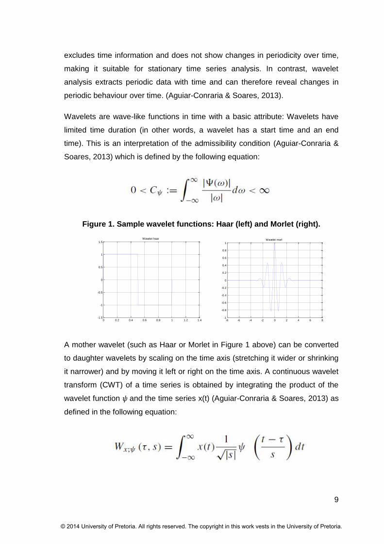
Figure 1. Sample wavelet functions: Haar (left) and Morlet (right).
A mother wavelet (such as Haar or Morlet in Figure 1 above) can be converted
to daughter wavelets by scaling on the time axis (stretching it wider or shrinking
it narrower) and by moving it left or right on the time axis. A continuous wavelet
transform (CWT) of a time series is obtained by integrating the product of the
wavelet function ψ and the time series x(t) (Aguiar-Conraria & Soares, 2013) as
defined in the following equation:
0 0.2 0.4 0.6 0.8 1 1.2 1.4-1.5
-1
-0.5
0
0.5
1
1.5Wavelet haar
-8 -6 -4 -2 0 2 4 6 8-1
-0.8
-0.6
-0.4
-0.2
0
0.2
0.4
0.6
0.8
1Wavelet morl
© 2014 University of Pretoria. All rights reserved. The copyright in this work vests in the University of Pretoria.

10
The continuous wavelet transform W is a function of the position in the time
series (τ) and the scale (s).
The wavelet transform operates in a moving time window on the time series.
Therefore the exact location in time of an exact scale cannot be known. A
Heisenberg box of the wavelet transform with a +/- standard deviation around a
point in scale and time can be constructed (Aguiar-Conraria & Soares, 2013).
Longer scales or periods (or lower frequency) have less certainty about the time
location and vice versa.
Aguiar-Conraria and Soares (2013) assert that although continuous wavelet
analysis is computationally more intensive, continuous wavelets are best suited
for financial time series analysis as the results are easier to interpret
graphically. According to Ahuja, Lertrattanapanich and Bose (2005), the
selection criteria for wavelet types when doing financial time series analysis
were (then) not well defined. Since then, some analysis has been done with
discrete wavelet transforms (Crowley, 2007) and maximum overlap discrete
wavelet transforms (Gallegati, 2008). For prediction models, the discrete
wavelet is the transform of choice (Zhu, Wang & Fan, 2014), as prediction
models work with discrete data as input (Ortega & Khashanah 2014); the
discrete wavelet transform contains the same information as the continuous
wavelet transform; it can be computed faster than the fast Fourier transform and
it can de-correlate time series (Percival & Walden, 2006, p.19).
2.8 Wavelet analysis of time series
Wavelets have been used to study various types of time series as indicated in
the examples below.
2.8.1 Natural cycles
A wavelet regression algorithm was used by Kisi (2010) for stream flow
prediction. The historic data was decomposed with the discrete wavelet
transform. Thereafter each scale’s time signal was separately reconstructed. A
regression was fitted between the separate scales’ time signals and the stream
flow, with noisy scale components discarded.
© 2014 University of Pretoria. All rights reserved. The copyright in this work vests in the University of Pretoria.

11
Zhu et. al. (2014) used a maximum overlap discrete wavelet transform – auto
regressive moving average (MODWT-ARMA) algorithm to predict daily rainfall.
They found MODWT-ARMA to outperform other forecasting models.
2.8.2 Economic cycles
Aguiar-Conraria and Soares (2011), applied wavelets to industrial production
index data and thereby identified patterns of synchronous business cycles
between countries in and around the European Union. These cycles change
over time. Dar, Samantaraya and Shah (2013) investigated whether the spread
between long- and short term interest rates (yield spread) predicts economic
activity in India. They found that yield spread predicts economic activity in long
time scales. A metal price forecast algorithm was devised by Kriechbaumer et
al. (2014). They combined wavelets with an autoregressive integrated moving
average filter (ARIMA) and improved the forecasting accuracy of the ARIMA
filter significantly.
Discrete wavelet decomposition was used in conjunction with autoregressive
filtering by Renaud, Starck and Murtagh (2005) to predict financial futures and
web site access. They adapted the wavelet transform to solve the wavelet
function on the edge so it can be used for prediction filters.
2.8.3 Electricity prices
A wavelet-auto regressive integrated moving average (ARIMA) electricity price
forecasting model was devised by Conejo, Plazas, Espinola and Molina (2005).
They decomposed historic prices with a discrete wavelet transform. Their next
step was to predict the future values of the decomposed series with the ARIMA
filter. An inverse wavelet transform was applied to the predicted decomposed
components to yield the forecast. Shrivastava and Panigrahi (2014) developed
an electricity price forecast algorithm by combining wavelets with an extreme
learning machine, while Voronin & Partanen (2014) combined wavelets with
ARIMA and neural networks.
© 2014 University of Pretoria. All rights reserved. The copyright in this work vests in the University of Pretoria.

12
2.8.4 Rates of exchange
Bekiros and Marcellino (2013) investigated co-movement and causal links
between the dollar, euro, pound and yen with daily data over 11 years. They
compared wavelet analysis with other methods and found wavelets useful for
predictions over any time span (Bekiros & Marcellino, 2013). Gençay, Selçuk
and Whitcher (2001) analysed scale (frequency) properties of the volatilities in
the exchange rates mark/dollar and yen/dollar. They applied wavelets to
exchange rate data from 1986 until 1996 sampled at 20 minute time intervals.
Insignificant cross correlation in volatility was observed on intraday level. Daily
volatility cycles dominated and longer term correlations were observed (Gençay
et al., 2001). These daily cycles are in agreement with the results of Heston et
al. (2010).
2.8.5 Share prices
Gallegati (2008) used MODWT to compare the DJIA and US Industrial
production index with monthly data in the period 1961 to 2006. They found that
production growth rate shows long memory dynamics while stocks shows short
memory and that stocks leads industry production by 16 months and longer.
Morris, Van Vuuren and Styger (2009) analysed seven share prices on the JSE
as well as the ALSI 40 index using daily closing prices through 2006 and 2007
with wavelets and a Markov model. Long memory behaviour was identified,
which constituted evidence against the weak-form efficient market hypothesis.
Wavelets and candlestick algorithms were combined by Li and Kuo (2008) in a
self-organising map to create a trading algorithm. It was tested with the Taiwan
weighted stock index with daily data from 1991 to 2002. The combined wavelet-
candlestick algorithm performed better than the algorithm without the wavelet
component.
In similar vein, Schlüter and Deuschle (2010) devised forecasting algorithms
using different wavelets and ARIMA filters. Two methods of incorporating
wavelet prediction were tested on different financial time series with daily price
data in the period 2007 to 2009. These were de-noising plus ARIMA, and
© 2014 University of Pretoria. All rights reserved. The copyright in this work vests in the University of Pretoria.

13
decomposing plus ARIMA on the decomposed scale components. The test
series consisted of a share price (Deutshe Bank), oil price (WTI), rate of
exchange (euro/dollar) and daily power prices in the UK. There were mixed
results. In the case of a large random component, wavelets added little value. If
the long term structure dominated, a de-noising approach with ARIMA was
found to be the best algorithm. In cases with dominant cycles, wavelet
decomposed scale combined with ARIMA gave the best results.
Benhmad (2013) correlated world stock market indices from 2005 to 2011 at
different scales. The markets could be classified as highly correlated, middle
correlated and less correlated and the correlation dynamics were found to be
time dependant. Dependency scales (frequencies) changed after the
bankruptcy of Lehman Brothers bank in 2008 (Benhmad, 2013).
2.8.6 Intraday share prices
A wavelet neural network prediction algorithm was devised by Ortega &
Khashanah (2014). The algorithm used high and low share prices in one minute
intervals as input and decomposed the prices with Haar maximum overlap
discrete wavelet transform (MODWT). The transform was used as input to a
neural network, which predicted log returns one-, three- and five minutes ahead.
2.9 Measures of algorithmic success
The purpose of this study was to use wavelets to extract cyclic components in
financial price series to predict share price movement. Measures of success
would be whether an algorithm can predict the share prices better, and whether
the algorithm can ensure superior returns.
The Wilcoxon signed-rank test is nonparametric and enables comparison of
matched pairs (Hines & Montgomery 1980, p.311). Therefore this test would be
suitable to compare the performances of different prediction and trading
algorithms at recurring times.
A risk when comparing algorithms using a specific data set is data snooping.
Data snooping occurs when a data set is re-used to compare models. With re-
© 2014 University of Pretoria. All rights reserved. The copyright in this work vests in the University of Pretoria.

14
used data, results may be due to chance rather than performance of the model
(White, 2000).
2.10 Conclusion of literature review
Technical trading is being performed more and more on an intraday basis
(Schulmeister, 2009) at higher turn-around times (Hasbrouck & Saar, 2013).
Although the order book is of paramount importance for high frequency trading
(Hasbrouck & Saar, 2013; Treleaven et al., 2013; Mackenzie, 2014), algorithms
based on historic price and volume data can still be employed at recurring time
intervals (Schulmeister, 2009; Ortega & Khashanah, 2014).
Asset price cycles, the changes in their periods over time and their co-
movements can be studied with wavelets (Aguiar-Conraria & Soares, 2013).
Wavelets can also be employed to improve prediction algorithms for prices of
commodities (Kriechbaumer et al., 2014) and shares (Schlüter & Deuschle,
2010). Transaction cost can be the make or break factor for trading algorithms
at all time scales (Schulmeister, 2009; Brogaard et al., 2012).
No literature was found regarding the application of wavelet analysis to intraday
trading. This research could contribute in this domain.
© 2014 University of Pretoria. All rights reserved. The copyright in this work vests in the University of Pretoria.

15
Chapter three - Research hypotheses
The gold price can go up or down, but not necessarily in that order – Clem
Sunter.
The purpose of the research was to determine whether wavelet based
algorithms can improve the performance of intraday trading algorithms. The
trading algorithms investigated, each consisted of two parts: the first part
performed share price prediction one and two time steps ahead and the second
part traded based on the prediction.
The performances of the share price prediction algorithm were compared based
on the accuracy of the prediction one and two time steps ahead as well as on
the directional accuracy at the same time steps. Two hypotheses were therefore
formulated to test the prediction performances.
Trade performances were compared by means of two additional hypotheses.
The third hypothesis was used to determine whether wavelet based algorithms
improve intraday trade performances. The fourth hypothesis was used to
compare the trading performances of the intraday trade algorithms with the
baseline of a buy-and-hold approach.
3.1 Hypothesis A
Ha0: Wavelet based share price prediction algorithms do not improve share
price prediction accuracy on an intraday scale.
Ha1: Wavelet based share price prediction algorithms improve share price
prediction accuracy on an intraday scale.
3.2 Hypothesis B
Hb0: Wavelet based algorithms do not improve the accuracy of predicting the
direction of share price movement on an intraday scale.
Hb1: Wavelet based algorithms improve the accuracy of predicting the direction
of share price movement on an intraday scale.
© 2014 University of Pretoria. All rights reserved. The copyright in this work vests in the University of Pretoria.

16
3.3 Hypothesis C
Hc0: Wavelet based share price prediction algorithms do not improve the
performance of intraday trading algorithms.
Hc1: Wavelet based share price prediction algorithms improve the performance
of intraday trading algorithms.
3.4 Hypothesis D
Hd0: Intraday trade algorithms do not perform better than buy-and-hold.
Hd1: Intraday trade algorithms perform better than buy-and-hold.
© 2014 University of Pretoria. All rights reserved. The copyright in this work vests in the University of Pretoria.

17
Chapter four - Research methodology
Eenvoud is die vreugde van die lewe (Simplicity is the joy of life) – Jannie du
Toit.
4.1 Introduction
The research methodology aim was to facilitate the comparison of the
performance of selected prediction algorithms for the purpose of trading. To this
end, a stepwise process was followed. Share price data was obtained and
prepared for application of the algorithms. The next step was to sample the
share prices in specific time intervals. Thereafter the data was divided: The first
half was allocated to the algorithm learning process and the second half to
testing. Teaching the different algorithms was the next step. This was followed
by testing the algorithms regarding prediction accuracy and trading
performance. The final step was to compare the algorithm performances. The
remainder of this chapter contains detail regarding this process.
4.2 Research philosophy
The research philosophy was positivism (Saunders & Lewis, 2012, p.104).
Structured methods were used that can be re-used on other data sets. The
research approach was deductive. The five sequential stages for deductive
research were applied, (Saunders & Lewis, 2012, p.108) including the
hypotheses statements; employment of a data analysis method resulting in the
acceptance/rejection of the hypotheses; comparing the results with previous
research and current theory to either confirm current theory or propose an
adaptation. The study was explanatory and quantitative (Saunders & Lewis,
2012, p.113).
4.3 Unit of analysis
The unit of analysis was a trade (a transaction to effect change of ownership of
shares) on the JSE. The population consisted of all the trades on the JSE. Each
trade had a price, volume and associated date and time of the transaction.
© 2014 University of Pretoria. All rights reserved. The copyright in this work vests in the University of Pretoria.

18
4.4 Data source
The Centre of Business Mathematics and Informatics of the North West
University, records data of all share trades on the JSE. The time resolution of
their recordings is one second. They supplied the trade data of the four selected
shares through 2013 (De Jongh, D., personal communication, August 26,
2014).
4.5 Data preparation
The data preparation consisted of sorting the trade data in time sequence,
reading it into Matlab and removing outliers. Price data points that were clearly
separate from the remainder of the price data (outliers) were considered
recording errors (Bisgaard & Kulahci, 2011, p.89) and were removed from the
data set.
4.6 Sampling
Sampling was done on various levels. The first level of sampling was to select
the time period – the year 2013. The second level of sampling was to select
specific shares - BTI (British American Tobacco), MTN, NPN (Naspers) and
SBK (Standard Bank). These shares were selected as they were the ones with
the largest market capitalisation in their respective industries.
The third sampling filter selected only those transactions that occurred within
the trading hours of the JSE (09h00 to 17h00) on the 250 trading days during
2013. As the last public trades occurred 10 minutes before closing time, the
trading hours were taken as 09h00 to 16h50. No special consideration was
given with respect to the days when the JSE opened after 09h00 or closed
earlier than 16h50.
Trades occur at random time intervals. One option would have been to analyse
the trades in the order of occurrence, tick by tick. This would have had the
advantage that no information would be ignored. The disadvantages of the tick
by tick approach would be that the number of data points to analyse would be
very large and that time-based patterns would be ignored.
© 2014 University of Pretoria. All rights reserved. The copyright in this work vests in the University of Pretoria.

19
The fourth sampling filter was therefore used to group the transactions in time
slots of different lengths. The selected time lengths were one, two, five and ten
minutes. The time slots were chosen to find a balance between a relative quick
reaction to market events (one minute) and minimising the number of time slots
where no price changes occurred.
The price associated with the last trade that occurred in each time slot was
used. In cases of time slots without trades, the most recent trade price was
used. This is in agreement with the market perception that the current price of a
share is the price of the most recent trade. Examples of other studies on
intraday price patterns applied sampling periods ranging from sub-second
(Cont, 2011) to 20 seconds (Gross-Klussmann & Hautsch, 2011), one minute
(Ortega & Khashanah, 2014), five minutes (Duvinage, Mazza and Petitjean,
2013 and Yamamoto, 2012) and 30 minutes (Heston, Korajczyk & Sadka,
2010).
The sampling resulted in time series of trade prices through 250 trade days in
2013 as shown in Table 1 below.
Table 1. Sampling intervals and the number of trade data points
Sampling interval
(minutes)
Number of trade
days
Number of price data points per
day
Number of price data
points through the year
Number of price data points for algorithm training
Number of price data points for algorithm
testing
1 250 470 117 500 58 750 58 750
2 250 235 58 750 29 375 29 375
5 250 94 23 500 11 750 11 750
10 250 47 11 750 5 875 5 875
4.7 Data splitting
The data was split in two halves: a “training part” and a “testing part”
(Montgomery, Jennings & Kulahci, 2008). The first half (2 January 2013 until 2
July 2013) was used for training the prediction algorithms (fitting models) and
the second half (3 July 2013 until 31 December 2013) for testing the algorithms
(forecasting and application of the trading algorithm).
© 2014 University of Pretoria. All rights reserved. The copyright in this work vests in the University of Pretoria.

20
4.8 Models for price prediction
Three basic models were used for price prediction and a dual algorithm for
trading. The prediction models were applied to predict prices one and two time
steps ahead, as this was the requirement of the trading algorithm. A trade
strategy of buy-and-hold served as a reference regarding financial performance.
Two of the models utilised wavelets. These contained sub-models whereby a
limited number of wavelet components would be used in the sub-model
prediction algorithms.
4.8.1 ARMA
Autoregressive moving average (ARMA) modelling is based on the assumption
that a future value of a time series has a relation to previous values (via the
autoregressive or AR part), plus a relation to previous and present random
inputs (via the moving average or MA component) (Bisgaard & Kulahci, 2011, p.
59-60). ARMA models can be fitted to time series if the mean is constant. If this
is not the case, the difference operator can be applied until the time series
mean is constant and the ARMA model can then be fitted to the difference time
series.
Selecting the order of the ARMA model to fit to a time series is often done by
analysing the autocorrelation function and the partial autocorrelation function of
the time series. Skill is required in pattern recognition that serves as guidance in
the selection of good models (Bisgaard & Kulahci, 2011, p. 60).
An alternative is to select the best ARMA model based on a measure. The
Bayesian information criterion (BIC) is suitable in cases of larger samples to
identify parsimonious models (Bisgaard & Kulahci, 2011, p. 164). BIC is
calculated as follows:
BIC ≈ n ln (a2) + r ln (n).
In this equation, n is the number of observations, a2 is the estimate of the
residual variance and r is the number of parameters used in the model
(Bisgaard & Kulahci, 2011, p. 164).
© 2014 University of Pretoria. All rights reserved. The copyright in this work vests in the University of Pretoria.

21
The BIC was applied as an automated criterion in all ARMA model selections of
this study, even though this approach is not recommended by Bisgaard &
Kulahci (2010, p. 164), This approach is practical for the real-life application of
the methods, as manual model selection for a large number of shares will not
be feasible.
A further restraint was applied in that all ARMA model orders were limited to
ARMA(4,4) (four autoregressive lags with four moving average lags). This was
done after observing that the relative change in the BIC value with increased
model order diminishes after three to four lags. In addition, this limit was
consistent with an approach of finding parsimonious models and not to over fit
(Bisgaard & Kulahci, 2011, p. 156).
The ARMA models were fitted on the training part of the data (first half) using
the estimate.m Matlab function. BIC values were calculated with the aicbic.m
function. The models with the lowest BIC scores were selected each time.
4.8.2 Wavelet-ARMA
Overview
The wavelet-ARMA model firstly utilised wavelets to decompose the time series
into different scale (or frequency) components. ARMA models were then fitted
to the individual scale components and the next time step values were predicted
for the wavelet components. The predicted share price was calculated as the
sum of selected wavelet component predictions. This approach was a
combination of parts of methods applied by Kisi (2010) and that of Schlüter and
Deuschle (2010) and Kriechbaumer et al (2014).
Wavelet
The continuous wavelet is useful for the graphical presentation of cycles over
time (Percival & Walden, 2006, p.12). However, it is the discrete wavelet
transform that is applied in prediction algorithms. The main reasons for using
the discrete wavelet transform are that the discrete wavelet transform contains
the same information as the continuous wavelet transform; it can be computed
© 2014 University of Pretoria. All rights reserved. The copyright in this work vests in the University of Pretoria.

22
faster than the fast Fourier transform and it can de-correlate time series
(Percival & Walden, 2006, p.19).
In this study, the Haar wavelet function was used. Although Kriechbaumer et. al.
(2014) found the performance of wavelet-ARIMA forecasting techniques
dependant both on the wavelet function and on the decomposition method, the
selection of Haar was based on the experience of Schlüter and Deuschle
(2010). They found smaller prediction errors with wavelet-ARIMA forecasting
algorithms of share prices when using Haar-based wavelets than with
Daubechies 4 wavelets.
The last 2n samples in the learning series was separated for the wavelet-ARMA
model fit, with n the largest possible integer. This was done to comply with the
wavelet algorithm requirement for a dyadic (2n, with n being a positive integer)
number of samples.
The discrete wavelet transform (DWT) of the log-return of the prices, was
calculated at the sampling intervals with the Matlab swt.m function. Five levels
of decomposition were used with the resulting decomposition scales shown in
Table 2 below. The inverse discrete wavelet transform was subsequently
applied separately to each of the five detail scales plus the approximation scale
with the Matlab function iswt.m. The result was six time signals, each containing
a specific scale component of the log return series. The sum of these six signals
equals the original log return signal.
Table 2. Scales and the sampling intervals
Scale level 1 2 3 4 5
Sampling interval
(minutes)
Decomposition scale (minutes)
1 2 4 8 16 32
2 4 8 16 32 64
5 10 20 40 80 160
10 20 40 80 160 320
© 2014 University of Pretoria. All rights reserved. The copyright in this work vests in the University of Pretoria.

23
ARMA
The next step was to fit separate ARMA models to each of these six time
signals. In this case, the limits for AR and MA lags were two of each. The BIC
selection criterion was also applied to select the most suitable model.
Prediction
During the test period, the prediction of two time steps ahead log return was
done as follows:
The 32 samples up to the required prediction time spot were used to apply the
discrete wavelet transform to five detail levels plus the approximation level. The
inverse discrete wavelet transform was then applied separately to each scale
(or level) component. The next two values for each of the series were predicted
with the ARMA models.
Six different wavelet-ARMA predictions of the log return at the time steps one
and two ahead were realised in this way. The first prediction consisted of the
sum of all six scale components, the second was the sum of scales 2 to 6, the
third the sum of scales 3 to 6 and so on. The prices for the next 2 time steps
ahead were calculated as the current price plus the predicted log returns.
4.8.3 Wavelet regression
Overview
The wavelet regression model was based on the approach of Kisi (2010).
Firstly, wavelets were used to decompose the time series into different scale (or
frequency) components. Secondly, a multiple linear regression model was
applied using the scale components as input and the one and two-step ahead
log return values as output. The predicted log return was calculated as the
regression fit of the preceding decomposed wavelets.
© 2014 University of Pretoria. All rights reserved. The copyright in this work vests in the University of Pretoria.

24
Wavelet
The same wavelet function and process of wavelet analysis was applied as for
the wavelet-ARMA case.
Regression
The regression algorithm used the six wavelet-decomposed time series as input
to fit to the one and two step ahead log return series. Six different predicted
values for the log return were obtained, using the same logic as in the wavelet-
ARMA prediction algorithm.
Six sets of price predictions were realised in the same fashion as with the
wavelet-ARMA method. The first prediction was a regression, based on all six
scale components, the second was a regression based on scales 2 to 6, the
third was a regression based on scales 3 to 6 and so on. The prices for the next
2 time steps ahead were calculated as the current price plus the predicted log
returns.
4.9 Trading algorithm
4.9.1 Buy-and-sell
Each of the prediction algorithms predicted the share price up to two time
periods into the future. The trade algorithm used these predictions with the
following logic:
If the predicted price, two periods ahead, was higher than the predicted
price, one period ahead (taking into account trading cost), the share was
bought in the next time period.
If a share was owned and the predicted price, two periods ahead, was
less than the predicted price, one period ahead, the share was sold in the
next time period.
The algorithm did not keep shares overnight. If a share was owned, the share
would be sold in the time slot that includes 16h30 and no further trade was done
for that day.
© 2014 University of Pretoria. All rights reserved. The copyright in this work vests in the University of Pretoria.
25
4.9.2 Short-and-close
As an alternative to buy-and-sell, a short-and-close approach was also
investigated. The decision logic is the same as for the buy-and-sell trade, with
one exception: The words “sell” or ”sold” are swapped with “buy” or “bought”. In
this case the short position was also closed at 16h30.
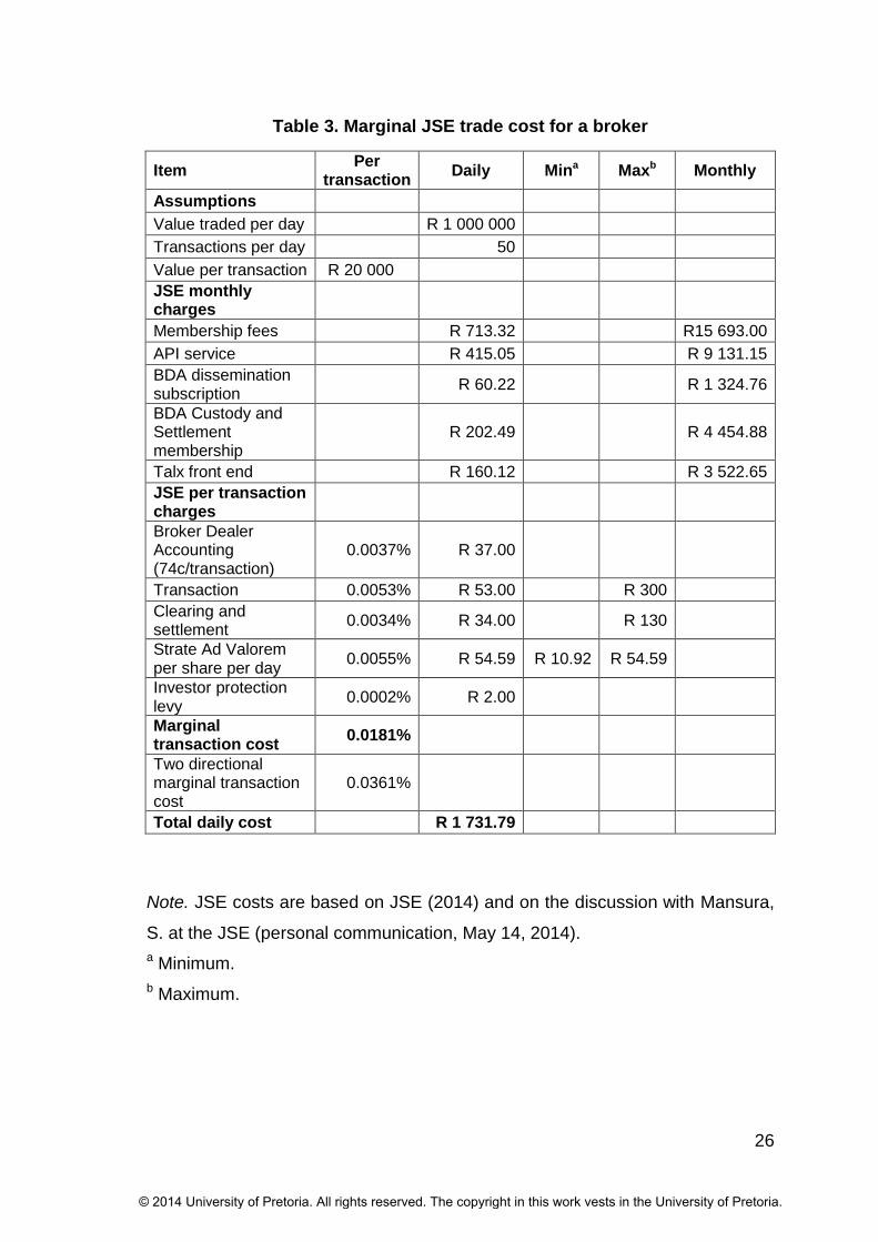
4.9.3 Trading cost
JSE stock brokers pay a variety of fees in order to trade (JSE, 2014).
Calculating the cost of a single trade is a challenge due to the myriad of monthly
fees and transaction costs. As the number of trades or the value of trades per
day increases (decreases), the trade cost per trade will decrease (increase).
The marginal trade cost percentage was estimated based on the JSE cost
brochure (JSE, 2014), assumptions as stated in Table 3 on page 26 and with
the aid of Mansura, S. at the JSE (personal communication, May 14, 2014).
Based on the calculations, a single direction trading cost of 0.018% was used
as part of the trading algorithm.
© 2014 University of Pretoria. All rights reserved. The copyright in this work vests in the University of Pretoria.
26
Table 3. Marginal JSE trade cost for a broker
Item Per
transaction Daily Mina Maxb Monthly
Assumptions
Value traded per day R 1 000 000
Transactions per day 50
Value per transaction R 20 000
JSE monthly charges
Membership fees R 713.32 R15 693.00
API service R 415.05 R 9 131.15
BDA dissemination subscription
R 60.22 R 1 324.76
BDA Custody and Settlement membership
R 202.49 R 4 454.88
Talx front end R 160.12 R 3 522.65
JSE per transaction charges
Broker Dealer Accounting (74c/transaction)
0.0037% R 37.00
Transaction 0.0053% R 53.00 R 300
Clearing and settlement
0.0034% R 34.00 R 130
Strate Ad Valorem per share per day
0.0055% R 54.59 R 10.92 R 54.59
Investor protection levy
0.0002% R 2.00
Marginal transaction cost
0.0181%
Two directional marginal transaction cost
0.0361%
Total daily cost R 1 731.79
Note. JSE costs are based on JSE (2014) and on the discussion with Mansura,
S. at the JSE (personal communication, May 14, 2014).
a Minimum.
b Maximum.
© 2014 University of Pretoria. All rights reserved. The copyright in this work vests in the University of Pretoria.
27
4.10 Comparisons
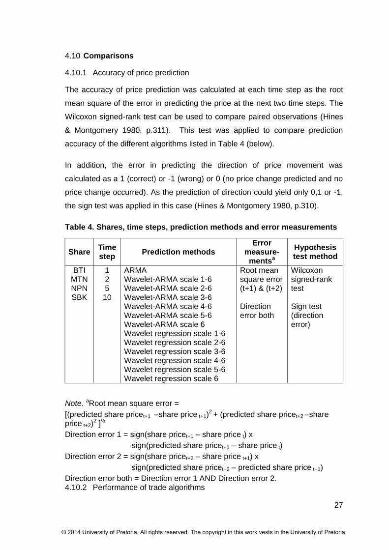
4.10.1 Accuracy of price prediction
The accuracy of price prediction was calculated at each time step as the root
mean square of the error in predicting the price at the next two time steps. The
Wilcoxon signed-rank test can be used to compare paired observations (Hines
& Montgomery 1980, p.311). This test was applied to compare prediction
accuracy of the different algorithms listed in Table 4 (below).
In addition, the error in predicting the direction of price movement was
calculated as a 1 (correct) or -1 (wrong) or 0 (no price change predicted and no
price change occurred). As the prediction of direction could yield only 0,1 or -1,
the sign test was applied in this case (Hines & Montgomery 1980, p.310).
Table 4. Shares, time steps, prediction methods and error measurements
Share Time step
Prediction methods Error
measure-mentsa
Hypothesis test method
BTI MTN NPN SBK
1 2 5
10
ARMA Wavelet-ARMA scale 1-6 Wavelet-ARMA scale 2-6 Wavelet-ARMA scale 3-6 Wavelet-ARMA scale 4-6 Wavelet-ARMA scale 5-6 Wavelet-ARMA scale 6 Wavelet regression scale 1-6 Wavelet regression scale 2-6 Wavelet regression scale 3-6 Wavelet regression scale 4-6 Wavelet regression scale 5-6 Wavelet regression scale 6
Root mean square error (t+1) & (t+2) Direction error both
Wilcoxon signed-rank test Sign test (direction error)
Note. aRoot mean square error =
[(predicted share pricet+1 –share price t+1)2 + (predicted share pricet+2 –share
price t+2)2 ]½
Direction error 1 = sign(share pricet+1 – share price t) x
sign(predicted share pricet+1 – share price t)
Direction error 2 = sign(share pricet+2 – share price t+1) x
sign(predicted share pricet+2 – predicted share price t+1)
Direction error both = Direction error 1 AND Direction error 2. 4.10.2 Performance of trade algorithms
© 2014 University of Pretoria. All rights reserved. The copyright in this work vests in the University of Pretoria.
28
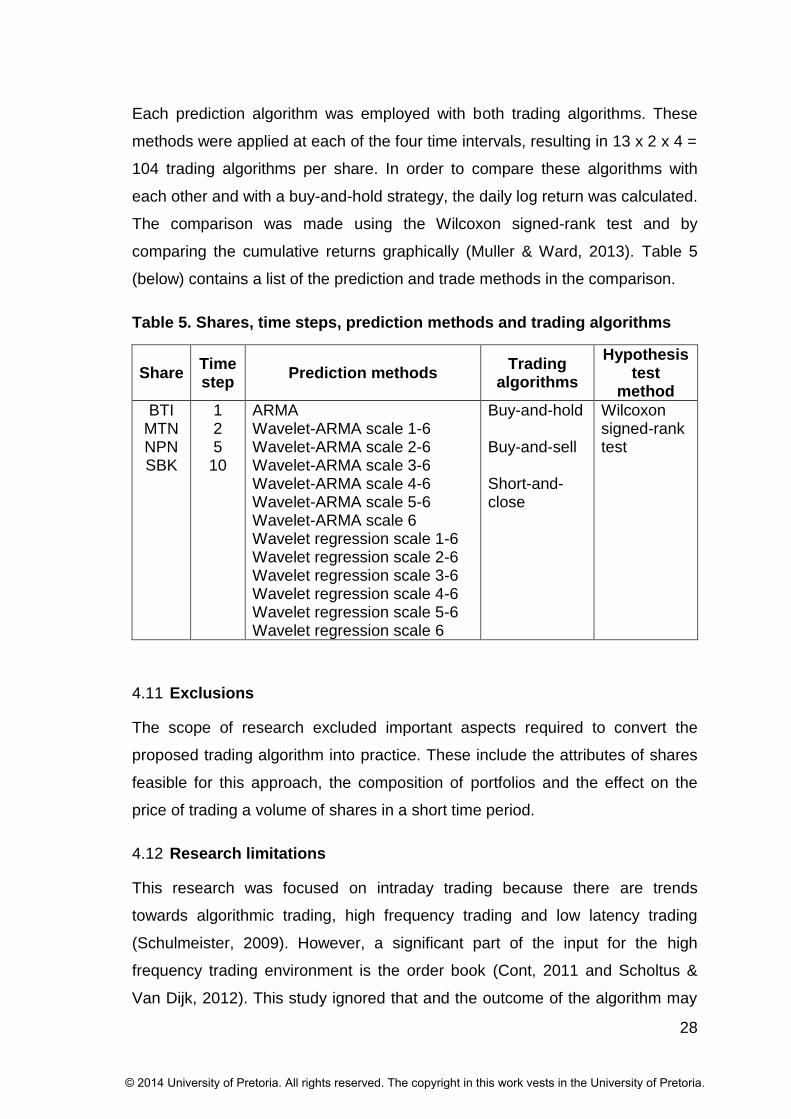
Each prediction algorithm was employed with both trading algorithms. These
methods were applied at each of the four time intervals, resulting in 13 x 2 x 4 =
104 trading algorithms per share. In order to compare these algorithms with
each other and with a buy-and-hold strategy, the daily log return was calculated.
The comparison was made using the Wilcoxon signed-rank test and by
comparing the cumulative returns graphically (Muller & Ward, 2013). Table 5
(below) contains a list of the prediction and trade methods in the comparison.
Table 5. Shares, time steps, prediction methods and trading algorithms
Share Time step
Prediction methods Trading
algorithms
Hypothesis test
method
BTI MTN NPN SBK
1 2 5
10
ARMA Wavelet-ARMA scale 1-6 Wavelet-ARMA scale 2-6 Wavelet-ARMA scale 3-6 Wavelet-ARMA scale 4-6 Wavelet-ARMA scale 5-6 Wavelet-ARMA scale 6 Wavelet regression scale 1-6 Wavelet regression scale 2-6 Wavelet regression scale 3-6 Wavelet regression scale 4-6 Wavelet regression scale 5-6 Wavelet regression scale 6
Buy-and-hold Buy-and-sell Short-and-close
Wilcoxon signed-rank test
4.11 Exclusions
The scope of research excluded important aspects required to convert the
proposed trading algorithm into practice. These include the attributes of shares
feasible for this approach, the composition of portfolios and the effect on the
price of trading a volume of shares in a short time period.
4.12 Research limitations
This research was focused on intraday trading because there are trends
towards algorithmic trading, high frequency trading and low latency trading
(Schulmeister, 2009). However, a significant part of the input for the high
frequency trading environment is the order book (Cont, 2011 and Scholtus &
Van Dijk, 2012). This study ignored that and the outcome of the algorithm may
© 2014 University of Pretoria. All rights reserved. The copyright in this work vests in the University of Pretoria.

29
therefore be sub-optimal at best for intraday applications. Furthermore, intraday
profits seldom exceed the 0.4% to 0.7% trading costs of non-stock broker
traders (Du Plessis, 2013). Therefore, intraday algorithms proposed herein are
suitable only in cases of lower trading cost that a stock broker may experience,
for instance as calculated in Table 3 on page 26.
The research had limitations regarding validity and reliability. Validity is an
indication of how well the data collection methods match the intended purpose
and whether the research findings are supported by the research (Saunders &
Lewis, 2012, p.127). Reliability refers to the repeatability of the research, or
whether the data collection and analysis methods will result in consistent
findings (Saunders & Lewis, 2012, p.128).
Validity is limited as the research was done using specific share data from the
JSE over a specific time period. It may not be applicable to other time periods or
to other shares listed on the JSE or elsewhere. Validity is further limited by
sampling the last price of the selected cycle, as this may have hidden some
attributes of the trade cycles.
The research is also limited in terms of the parameters chosen. Only two
wavelet based algorithms were investigated. Only Haar wavelets were used.
Scales were limited to five plus the approximate scale. ARMA orders were
limited. Only four time steps were investigated. Only time steps on the minute
were investigated. Validity may have been compromised further as no special
consideration was given to the possible effect of data snooping.
Reliability may have been compromised if the data base contained errors or
omissions. In addition, applying the research to a specific time period and
analysing only selected shares may have limited the repeatability of results and
therefore the reliability.
© 2014 University of Pretoria. All rights reserved. The copyright in this work vests in the University of Pretoria.
30
Chapter five – Results
Prediction is difficult, especially about the future - Niels Bohr.
5.1 Introduction
The results include an overview of the sample data, the modelling parameters
and the results of the hypothesis tests. To start with, descriptions of the sample
share price data are presented. This is followed by the prediction models fitted
to each of the algorithms using the training part of the data. The results of the
prediction algorithms’ comparative tests are shown next based on the minimum
error as well as the directional accuracy. Lastly, the results of the tests
regarding trading algorithm performances of the different methods are
presented.
5.2 Description of the sample share price data
The cumulative log returns of MTN, SBK, BTI and NPN through 2013 are shown
in Figure 2 on page 31. Table 6 on page 32 contains descriptive statistics
pertaining to the complete data set of all the JSE trades of the four shares
during 2013. Table 7 on page 32 contains descriptive statistics relating to the
log returns and the number of transactions per day.
The analysis was done using time intervals of one, two, five and ten minutes
respectively. Descriptive statistics of the number of trades and the log returns
per time interval are shown in Table 11 on page 54.
© 2014 University of Pretoria. All rights reserved. The copyright in this work vests in the University of Pretoria.

31
Figure 2. Cumulative log returns of share prices through trade days of 2013.
Note. The trade days commenced on 2 January 2013 and ended on 31
December 2013. It excluded weekends and public holidays, resulting in 250
trade days.
© 2014 University of Pretoria. All rights reserved. The copyright in this work vests in the University of Pretoria.
32
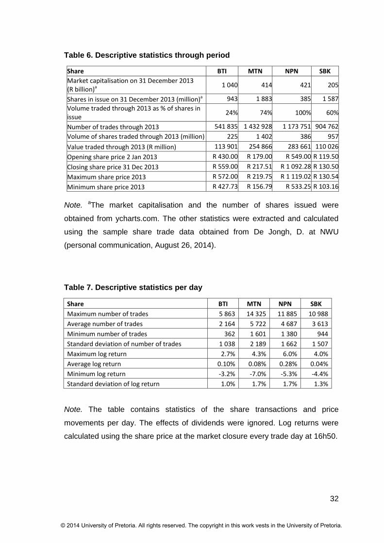
Table 6. Descriptive statistics through period
Share BTI MTN NPN SBK
Market capitalisation on 31 December 2013 (R billion)a
1 040 414 421 205
Shares in issue on 31 December 2013 (million)a 943 1 883 385 1 587
Volume traded through 2013 as % of shares in issue
24% 74% 100% 60%
Number of trades through 2013 541 835 1 432 928 1 173 751 904 762
Volume of shares traded through 2013 (million) 225 1 402 386 957
Value traded through 2013 (R million) 113 901 254 866 283 661 110 026
Opening share price 2 Jan 2013 R 430.00 R 179.00 R 549.00 R 119.50
Closing share price 31 Dec 2013 R 559.00 R 217.51 R 1 092.28 R 130.50
Maximum share price 2013 R 572.00 R 219.75 R 1 119.02 R 130.54
Minimum share price 2013 R 427.73 R 156.79 R 533.25 R 103.16
Note. aThe market capitalisation and the number of shares issued were
obtained from ycharts.com. The other statistics were extracted and calculated
using the sample share trade data obtained from De Jongh, D. at NWU
(personal communication, August 26, 2014).
Table 7. Descriptive statistics per day
Share BTI MTN NPN SBK
Maximum number of trades 5 863 14 325 11 885 10 988
Average number of trades 2 164 5 722 4 687 3 613
Minimum number of trades 362 1 601 1 380 944
Standard deviation of number of trades 1 038 2 189 1 662 1 507
Maximum log return 2.7% 4.3% 6.0% 4.0%
Average log return 0.10% 0.08% 0.28% 0.04%
Minimum log return -3.2% -7.0% -5.3% -4.4%
Standard deviation of log return 1.0% 1.7% 1.7% 1.3%
Note. The table contains statistics of the share transactions and price
movements per day. The effects of dividends were ignored. Log returns were
calculated using the share price at the market closure every trade day at 16h50.
© 2014 University of Pretoria. All rights reserved. The copyright in this work vests in the University of Pretoria.
33
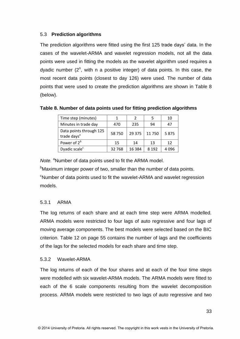
5.3 Prediction algorithms
The prediction algorithms were fitted using the first 125 trade days’ data. In the
cases of the wavelet-ARMA and wavelet regression models, not all the data
points were used in fitting the models as the wavelet algorithm used requires a
dyadic number (2n, with n a positive integer) of data points. In this case, the
most recent data points (closest to day 126) were used. The number of data
points that were used to create the prediction algorithms are shown in Table 8
(below).
Table 8. Number of data points used for fitting prediction algorithms
Time step (minutes) 1 2 5 10
Minutes in trade day 470 235 94 47
Data points through 125 trade daysa
58 750 29 375 11 750 5 875
Power of 2b 15 14 13 12
Dyadic scalec 32 768 16 384 8 192 4 096
Note. aNumber of data points used to fit the ARMA model.
bMaximum integer power of two, smaller than the number of data points.
cNumber of data points used to fit the wavelet-ARMA and wavelet regression
models.
5.3.1 ARMA
The log returns of each share and at each time step were ARMA modelled.
ARMA models were restricted to four lags of auto regressive and four lags of
moving average components. The best models were selected based on the BIC
criterion. Table 12 on page 55 contains the number of lags and the coefficients
of the lags for the selected models for each share and time step.
5.3.2 Wavelet-ARMA
The log returns of each of the four shares and at each of the four time steps
were modelled with six wavelet-ARMA models. The ARMA models were fitted to
each of the 6 scale components resulting from the wavelet decomposition
process. ARMA models were restricted to two lags of auto regressive and two
© 2014 University of Pretoria. All rights reserved. The copyright in this work vests in the University of Pretoria.

34
lags of moving average components each. The best models were selected
based on the BIC criterion. The number of lags and the coefficients of the lags
for the selected models for each share, time step and scale are shown in Table
13 on page 56 (BTI and MTN) and Table 14 on page 58 (NPN and SBK).
A sample graph with the wavelet components is shown in Figure 3 on page 70.
The time duration consists of trade days 55 to 125, comprising of 32 768 (215)
one minute time steps. Figure 4 on page 71 and Figure 5 on page 72 contain
the same graph zoomed in to 12 days and 2 days respectively in order to show
some detail. The higher volatility of share prices early and late in the trade day
(Cont et al., 2014) are clearly visible in these graphs.
5.3.3 Wavelet regression
The wavelet regression model started with the wavelet decomposition and
separation of scale components in the same way as was done in the case of the
wavelet-ARMA model. A regression was fitted thereafter, linking each scale
component shown in Figure 3 on page 70 to the next time step value of the log
return. The regression model for the second time step ahead linked the scale
components to the log return values at two time steps ahead. The regression
coefficients for one and two time steps ahead are shown in Table 15 on page
60. The table also shows the correlation coefficients (R2 statistics) for the first
and second time steps ahead regression models.
5.4 Prediction accuracy
The purpose of the accuracy measurements was to determine whether wavelet
based share price prediction algorithms improve share price prediction accuracy
on an intraday scale (Hypothesis Ha). The three prediction methods (ARMA,
Wavelet-ARMA and Wavelet regression) were applied to four shares and at four
sampling intervals (one, two, five and ten minutes) as summarised in Table 4 on
page 27.
The two wavelet-based algorithms each comprised of six variants. The basic
variants each utilised the combination of scales 1 to 6. The second variants
used scales 2 to 6 and so on, up to the sixth variants, which used only scale 6.
© 2014 University of Pretoria. All rights reserved. The copyright in this work vests in the University of Pretoria.

35
Prediction accuracies were measured by calculating the root mean square error
for one and two time steps ahead and the directional errors for both one and
two time steps ahead with the formulas indicated below Table 4 on page 27.
These values at each time step of the test data were used in the hypothesis
test. The averages of the root mean square values were also calculated and are
shown in Table 16 on page 61 for the cases outperforming ARMA.
The hypothesis regarding prediction accuracy was tested with the Wilcoxon
signed-rank test while the sign test was applied to test the hypothesis regarding
the prediction of direction. In each case, the confidence level was 95% and a
one-tailed test was conducted.
5.4.1 Prediction of share price accuracy
The hypothesis regarding prediction accuracy was tested per time step and per
share. Table 16 on page 61 contains the list of prediction methods with the root
mean square (RMS) of one and two time steps ahead prediction errors lower
than the ARMA method according to the Wilcoxon signed-rank test. Both tables
contain the means of the RMS errors and for reference, the means of the RMS
errors of the ARMA prediction methods.
Table 9. Rank of algorithms with lowest prediction error
Time step
Method & scale 1 2 5 10
ARMA 2 1 1 1
Wavelet-ARMA 6 1 2 2 2
Wavelet regression 6 3 3 3 3
Wavelet-ARMA 5 to 6 4 4 4 4
Wavelet regression 5 to 6 5 5 5 5
Note. Rank of 1 indicates the method outperforming most others based on the
Wilcoxon signed-rank test.
The results per share are combined in Table 9 (above) where the prediction
methods’ performances are ranked per time step. The ranking was done by
performing a Wilcoxon signed-rank test between each of the prediction methods
per time step and adding the results.
© 2014 University of Pretoria. All rights reserved. The copyright in this work vests in the University of Pretoria.

36
5.4.2 Prediction of direction accuracy
The hypothesis regarding prediction accuracy was also tested based on the
accuracy of the predicted direction of share price movement, per time step and
per share. Both time steps were considered simultaneously as this combination
impacted directly on the trading algorithm. Table 17 on page 62 contains the list
of prediction methods with both the predicted direction errors lower than the
ARMA method according to the Sign test. The table also contains the
percentages of the directions predicted correctly. The results of ARMA based
predictions are included for reference.
The results per share are combined in Table 10 (below) where the directional
accuracies of the prediction methods are ranked per time step. The ranking was
done by performing a sign test between each of the prediction methods per time
step and adding the results.
Table 10. Rank of algorithms performing best in predicting the direction of price changes of the next two time steps
Time step
Method & scale 1 2 5 10
Wavelet regression 2 to 6 1 1 1 1
Wavelet-ARMA 2 to 6 2 2 2 2
Wavelet-ARMA 3 to 6 3 3 3 3
Wavelet regression 3 to 6 4 4 4 4
Wavelet-ARMA 1 to 6 5 5
Note. Rank of 1 indicates the method outperforming most others based on the
sign test.
5.5 Trading performance
The trading performances of the algorithms were compared in order to
determine whether wavelet based algorithms improve trading performance
(Hypothesis Hb). Secondly, intraday trading algorithms were compared with
buy-and-hold (Hypothesis Hc). The test time period consisted of trade days 126
to 250.
© 2014 University of Pretoria. All rights reserved. The copyright in this work vests in the University of Pretoria.

37
The three prediction methods (ARMA, Wavelet-ARMA and Wavelet regression)
were applied to four shares and at four sampling intervals (one, two, five and
ten minutes), and combined with both buy-and-sell and short-and-close trading
algorithms. Buy-and-hold was added to the comparison. The methods are
summarised in Table 4 on page 27.
The trade algorithms would signal buy or sell (alternatively, short or close), or
retain the current position. For each trade the log return was calculated. Trade
fees of 0.018% per one direction transaction were incorporated. (The
calculation is shown in Table 3 on page 26.) The cumulative log return per day
was calculated. This allowed the comparison of the algorithms of all the time
steps.
In the case of buy-and-hold, no transaction fees were incorporated since the
0.036% two-way cost was considered as being negligible for the one trade. The
buy-and-hold daily returns were calculated using the share prices at the end of
the first minute of each trading day.
The hypothesis regarding trading algorithm performance was tested with the
Wilcoxon signed-rank test. The confidence level was 95% and a one-tailed test
was conducted.
Table 18 on page 68 contains the list of predicting-trading algorithm
combinations that performed better than ARMA, buy-and-hold, indicated for the
applicable shares. The comparisons were made using the Wilcoxon signed-rank
test. Table 19 on page 69 lists the predicting-trading algorithm combinations
having positive cumulative returns over the test period, with their respective
cumulative log returns per share over the test period.
An alternative approach to compare the performances was also investigated.
The cumulative returns of the trading methods were calculated and graphically
compared (Muller & Ward, 2013) in Figure 6 on page 73 to Figure 9 on page 76.
The performances of the trade algorithms with the highest cumulative returns
for each share are shown.
© 2014 University of Pretoria. All rights reserved. The copyright in this work vests in the University of Pretoria.
38
5.6 Intraday trading algorithms vs. buy-and-hold
None of the intraday trading algorithms were found to perform better than buy-
and-hold according to the Wilcoxon signed-rank test. This result is confirmed in
the graphs showing the cumulative log returns (Figure 6 on page 73 to Figure 9
on page 76), where no significant out-performance of the intraday trading
algorithms can be observed.
5.7 Trading cost and number of transactions
The calculated marginal trading cost was 0.018% in one direction. (The
calculation is shown in Table 3 on page 26.) At this rate, two buy-and-sell
transactions (four trades) per day (or 500 trades through the 125 day test
period) would result in a cumulative return of minus 9.4% over the test period of
125 days (six months). The number of transactions per scale is shown in Figure
10 on page 77. It is clear that the lower the scale (higher frequency), the more
transactions the trading algorithm invoked and the higher the cumulative trading
cost would be.
The last column of Table 19 on page 69 contains the number of profitable
trades/number of trades through the 125 day test period for the cases with a
profitable cumulative return. The maximum number of transactions in this table
is 518, or 4 transactions per day, supporting the argument that the cost of the
high volume of transactions was instrumental in the lack of performance of trade
algorithms utilising wavelets lower scales (higher frequencies).
5.8 Conclusion of the results chapter
The results of hypotheses tested were as follows:
Ha0: Wavelet based share price prediction algorithms do not improve share
price prediction accuracy on an intraday scale.
The hypothesis Ha0 cannot be rejected.
© 2014 University of Pretoria. All rights reserved. The copyright in this work vests in the University of Pretoria.

39
Hb0: Wavelet based algorithms do not improve the accuracy of predicting the
direction of share price movement on an intraday scale.
The hypothesis Hb0 can be rejected.
Hc0: Wavelet based share price prediction algorithms do not improve the
performance of intraday trading algorithms.
The hypothesis Hc0 can be rejected.
Hd0: Intraday trade algorithms do not perform better than buy-and-hold.
The hypothesis Hd0 cannot be rejected.
© 2014 University of Pretoria. All rights reserved. The copyright in this work vests in the University of Pretoria.
40
Chapter six - Discussion of results
We are looking for the needle in the haystack – Chris Muller.
6.1 Introduction
The main purpose of the research was to determine whether wavelet based
prediction algorithms can improve intraday trading algorithms. The fit of
algorithms are discussed first. Thereafter the results related to each hypothesis
are discussed. This chapter also includes a discussion on the effect of trading
costs.
6.2 Algorithm fit
The ARMA, wavelet-ARMA and wavelet regressive models were fitted using the
first half year of log returns. Half of the ARMA models fitted contained no
autoregressive components (Table 12 on page 55), indicating that randomness
overshadowed other effects in these log return series. This resulted in these
algorithms having no prediction power beyond a constant mean. This situation
occurred in only one of the ARMA model fits to the wavelet components (Table
13 on page 56 and Table 14 on page 58), indicating lower levels of randomness
in the decomposed series.
The R2 (coefficient of determination) values in the case of the wavelet
component regression fits to the next values of the log returns, are around 0.5
in cases of one time step ahead and around 0.4 in cases of two time steps
ahead (Table 15 on page 60). These R2 values indicate a relationship, albeit not
too strong.
6.3 Accuracy of price prediction
Hypothesis Ha0: Wavelet based share price prediction algorithms do not
improve share price prediction accuracy on an intraday scale.
This null hypothesis could not be rejected as it could not be shown that wavelet-
ARMA and wavelet regression algorithms outperformed ARMA in predicting the
prices at the next two time steps based on the root mean square (RMS)
© 2014 University of Pretoria. All rights reserved. The copyright in this work vests in the University of Pretoria.

41
measurement criteria. However, at a time step of 1 minute, in the cases of BTI
and NPN, wavelet-ARMA and wavelet regression methods at scales 6, 5-6 and
4-6 (lower frequencies) yielded lower RMS prediction errors on average than
ARMA (Table 16 on page 61).
In this study, the errors in predicting one and two time steps ahead were
combined. This was done because the purpose of the prediction was to serve
as input for the trading algorithm which used these two variables. This approach
of combining errors of time steps was not found in the literature and the results
may therefore not be strictly comparable with other studies. Nevertheless, the
result obtained in this study is in agreement with the results of Schlüter and
Deuschle (2010), who did not find improvements due to wavelets for all financial
time series they tested. The results herein however contradict the results of
other research that found that wavelet based forecasting improves prediction
accuracy (Kisi, 2010; Zhu et. al., 2014; Ortega & Khashanah, 2014).
6.4 Accuracy of direction prediction
Hb0: Wavelet based algorithms do not improve the accuracy of predicting the
direction of share price movement on an intraday scale.
This null hypothesis was rejected as the prediction of the direction of share
price movement was found to be improved by wavelet based methods. These
results are in agreement with the study of Ortega and Khashanah (2014) who
found wavelets to improve the directional prediction accuracy.
The list in Table 17 on page 62 indicates that wavelet based methods can
outperform ARMA for all the shares tested and at all the time scales. The best
performing methods utilise scales 2 to 6 and 3 to 6 (it includes higher frequency
scales) as indicated in Table 10 on page 36. This is in contrast with all the other
performance tests in this study, where methods with lower frequency scales
were found to perform better.
© 2014 University of Pretoria. All rights reserved. The copyright in this work vests in the University of Pretoria.
42
6.5 Trade algorithm performance
Hc0: Wavelet based share price prediction algorithms do not improve the
performance of intraday trading algorithms.
The null hypothesis was rejected in this case as the incorporation of wavelets in
the prediction algorithms was found to improve the intraday returns relative to
ARMA algorithms in specific cases of BTI, NPN and SBK shares (Table 18 on
page 68). In the case of MTN, no improvement was found. Although no results
of wavelet based trading algorithms were found in the literature, the results of
this study is in agreement with the finding of Schlüter and Deuschle (2010), who
found that wavelets can improve the prediction accuracy of financial time series
in some cases.
The best performing wavelet-based algorithms in trading had higher scales
(lower frequencies). This result is in agreement with the findings of Kisi (2010),
who omitted lower scales in prediction algorithms for improved accuracy. Trade
costs may have contributed to the results of this study: At lower scales (higher
frequencies), the trading algorithm invoked a higher number of trades per day
than in cases with higher scales. The associated higher cumulative trading
costs penalised the lower scales algorithms.
Almost all the trading algorithms with positive cumulative returns utilised the one
minute duration time interval (Figure 6 on page 73 to Figure 9 on page 76). The
exception is NPN, where the algorithms operating at 5 and 10 minute time
intervals performed better.
All the wavelet based algorithms with positive cumulative returns utilised the
short-and-close trading algorithm. This means the trade algorithm was profitable
when the prediction algorithm incorrectly predicted price and direction.
© 2014 University of Pretoria. All rights reserved. The copyright in this work vests in the University of Pretoria.
43
6.6 Buy and hold
Hd0: Intraday trade algorithms do not perform better than buy-and-hold.
The null hypothesis in this case could not be rejected as no intraday algorithm
was found to statistically outperform buy-and-hold over the test period. Selected
trade algorithms did however result in higher cumulative returns than buy-and-
hold through the test period (Figure 6 on page 73 to Figure 9 on page 76 and
Table 19 on page 69). This result is in agreement with the findings of Duvinage
et al. (2013), Yamamoto (2012) and Marshall et al. (2008).
The fact that the algorithms tested in this study did not outperform buy and hold,
do not negate the feasibility of intraday trading, as reported in various studies
(Schulmeister, 2009; Scholtus & Van Dijk, 2012; Hasbrouck & Saar, 2013;
Hagströmer & Nordén, 2013; Menkveld, 2013 and Mackenzie, 2014).
6.7 The effect of trading cost
The cost of trading played a significant part in the findings as the cumulative
negative return escalated as the number of trades increased. The significance
of trading costs was also reported by Schulmeister (2009), Brogaard et al.
(2012), Elkins McSherry (2012) and Du Plessis (2013).
6.8 Conclusion regarding the results
Intraday wavelet based prediction algorithms were found to improve the
performance of trade algorithms in some cases. The intraday algorithms could
not improve on a buy-and-hold strategy. A main driver in the performance of the
algorithms was trading cost.
© 2014 University of Pretoria. All rights reserved. The copyright in this work vests in the University of Pretoria.
44
Chapter seven – Conclusion
The first principle is that you must not fool yourself and you are the easiest
person to fool ― Richard Feynman.
7.1 Introduction
This research tested whether wavelet based algorithms can improve the
performance of intraday share trading algorithms. The trading algorithms
investigated each consisted of two parts: the first part performed share price
prediction and the second part traded shares based on the prediction. Three
types of prediction algorithms were employed: auto regressive moving average
(ARMA), wavelet-ARMA and wavelet regressive algorithms. The wavelet based
algorithms were further broken down by using up to 6 different levels of scales
in each of the algorithms.
These algorithms were applied to the trade data of four JSE shares through
2013. The first half year of data was used to fit algorithms while the tests were
conducted on the second half year of data
7.2 Main findings
The accuracy of the wavelet based share price prediction algorithms were found
not to outperform the autoregressive moving average algorithms. This result is
in agreement with that of Schlüter and Deuschle (2010), who found
improvements in the accuracy of price prediction due to wavelets only for some
of the financial time series they tested. The results herein however do not
support the findings of other research that found that wavelet based forecasting
improves prediction accuracy (Kisi, 2010; Zhu et.al., 2014; Ortega &
Khashanah, 2014).
The accuracy of predicting the direction the share price will move is important
for trade algorithms. This research found that accuracy of predicting price
direction was improved by wavelets, in agreement with the findings of Ortega
and Khashanah (2014). Specifically, inclusion of lower scale (higher frequency)
© 2014 University of Pretoria. All rights reserved. The copyright in this work vests in the University of Pretoria.
45
wavelet components as part of the prediction algorithms was found to improve
directional prediction accuracy.
Returns of the trade algorithm were found to have improved due to the
incorporation of wavelets in the prediction algorithms relative to ARMA
algorithms in specific cases. In the case of one share (MTN), no improvement
was found. No direct comparison with previous research was done as no results
of wavelet based trading algorithms were found in the literature. However, this
result is in agreement with the Schlüter and Deuschle (2010) finding that
wavelets can improve the prediction accuracy of financial time series in some
cases.
The best performing wavelet-based algorithms in trading had higher scales
(lower frequencies). This observation is in agreement with the findings of Kisi
(2010), who omitted lower scales in prediction algorithms for improved
accuracy.
None of the intraday algorithms were found to outperform buy-and-hold over the
test period. This result is in agreement with the findings of Duvinage et al.
(2013), Yamamoto (2012) and Marshall et al. (2008). The active practice of
intraday trading, albeit with different algorithms (Schulmeister, 2009; Scholtus &
Van Dijk, 2012; Hasbrouck & Saar, 2013; Hagströmer & Nordén, 2013;
Menkveld, 2013 and Mackenzie, 2014), however, contradicts the result.
Trade costs have a significant impact on the performance of intraday trades
(Menkveld, 2013; Scholtus & Van Dijk, 2012; Du Plessis, 2013). In this study, it
was observed that algorithms using lower scales (higher frequencies) invoked a
higher number of trades per day than in cases with lower scales. The
associated higher cumulative trading costs penalised the lower scales
algorithms.
7.3 Recommendations to industry
The growth of computerised trading implies continuing change to the stock
market trading industry. Industry should take cognisance of the growth of high
frequency trading and the associated algorithmic trading. High frequency
© 2014 University of Pretoria. All rights reserved. The copyright in this work vests in the University of Pretoria.
46
trading accounts for more than half the traded shares in the USA, more than
35% in the UK and in Canada (Aitken, Cumming & Zhan, 2014), more than 40%
in Germany (Reuters, 2013), while 17% of JSE trades occur via colocation
servers (JSE, 2014b) and are therefore likely high frequency trades. The JSE
colocation service started on 12 May 2014 (JSE, 2014b). In addition, the
increase in high frequency trading is causing changes in regulations (Reuters,
2013).
The options available when fitting models to financial data are boundless.
Industry should remain abreast of the modelling techniques and algorithms, like
wavelets, used in physical science and engineering.
Lastly, trading costs are expected to continue on a downward trend due to
growing opening of markets (globalisation) and increased competition between
exchanges (Menkveld, 2013). Lower trading costs make high frequency
algorithmic trading increasingly feasible.
7.4 Suggestions for future research
Intraday trading and the associated trade algorithms is a relative recent
phenomenon driving a significant part of the turnover of stock exchanges
(Aitken, Cumming & Zhan, 2014). Limited academic research has been
published in this regard (Chordia, Goyal, Lehmann & Saar, 2013). Commercial
secrecy issues surrounding trading algorithms could be a compounding factor.
Regulation of high frequency- and algorithmic trading is a work in process
(Reuters, 2013) towards which academic research can contribute.
The trading cost is a make-or-break factor for algorithmic trading (Menkveld,
2013). A comparison between the trading costs of different stock exchanges
and the changes in cost over time will yield valuable information for algorithmic
traders.
Wavelets can yield information on the co-movement of assets over time
(Aguiar-Conraria & Soares, 2013). A suggested research subject is to analyse
the co-movement of assets on an intraday scale with wavelets. Such
discoveries can improve prediction accuracies for improved trade algorithms.
© 2014 University of Pretoria. All rights reserved. The copyright in this work vests in the University of Pretoria.

47
A myriad of options exist when applying models to financial time series. An
option for further research is to refine the decisions made in this study. Options
include the following: Other durations for time steps; exploiting the daily volatility
cycle in the share prices (Scholtus & Van Dijk, 2012); using the period average
and/or high and/or low prices (Ortega & Khashanah, 2014) instead of the end of
period prices in the prediction; changing the limits of the maximum numbers of
coefficients in the auto-regressive moving average filters; changing the time
scales of the wavelet decompositions; changing the combinations of the scales
for prediction purposes; changing the wavelet filter and changing the samples.
A related issue is the trade algorithm. The algorithm applied in this research
was straightforward. The effect of a more elaborate algorithm with a slower
decision filter can be investigated. In addition, all the wavelet based algorithms
with positive cumulative returns utilised the short-and-close trading algorithm in
this research. This means the trade algorithm was profitable when the
prediction algorithm was wrong regarding the price predictions and directions.
The reason for this phenomenon could be investigated.
The best predictors of share price direction were found to be wavelet methods
utilising scales 2 to 6 and 3 to 6 (it includes higher frequency scales) as
indicated in Table 10 on page 36. This is in contrast with all the other
performance tests in this study, where methods with lower frequency scales
were found to perform better. The reason for this phenomenon could be further
investigated.
7.5 Concluding remarks
This research did not find that intraday trading algorithms outperform a buy-and-
hold strategy. However, intraday trading is a growing trend. As trading costs
come down due to competition between stock exchanges, the scope for
algorithmic trading will grow. Wavelet based algorithms can contribute to the
performance of trade algorithms.
© 2014 University of Pretoria. All rights reserved. The copyright in this work vests in the University of Pretoria.

48
References
Aguiar-Conraria, L., & Soares, M.J. (2011). Business cycle synchronization and
the Euro: a wavelet analysis. Journal of Macroeconomics,33(3), 477-489.
Aguiar-Conraria, L., & Soares, M. J. (2013). The continuous wavelet transform:
Moving beyond uni- and bivariate analysis. Journal of Economic Surveys.
DOI: 10.1111/joes.2012.
Ahuja, N., Lertrattanapanich, S., & Bose, N. K. (2005). Properties determining
choice of mother wavelet. IEE Proceedings-Vision, Image and Signal
Processing, 152(5), 659-664.
Aitken, M., Cumming, D., & Zhan, F. (2014). Trade Size, High Frequency
Trading, and Co-Location Around the World. European Journal of Finance,
forthcoming.
Barr, G. D. I., & Kantor, B. S. (2005). The impact of the rand on the value of the
Johannesburg Stock Exchange. Journal for Studies in Economics and
Econometrics, 29(2), 77.
Bekiros, S., & Marcellino, M. (2013). The multiscale causal dynamics of foreign
exchange markets. Journal of International Money and Finance, 33, 282-
305.
Belardi, A. A., Aguiar, R. A., & Fausto, S. (2012). Dollar and the stock market:
An approach using Haar wavelet. In First International Conference On
Analysis And Applied Mathematics: ICAAM 2012 (Vol. 1470, No. 1, pp. 218-
221). AIP Publishing.
Benhmad, F. (2013). Bull or bear markets: A wavelet dynamic correlation
perspective. Economic Modelling, 32, 576-591.
Betancourt, L., VanDenburgh, W. M., & Harmelink, P. J. (2011). Understanding
the 'Flash Crash.'. CPA Journal, 81(1), 40-45.
© 2014 University of Pretoria. All rights reserved. The copyright in this work vests in the University of Pretoria.

49
Bisgaard, S. & Kulahci, M. (2011). Time series analysis and forecasting by
example. Hoboken, New Jersey: John Wiley & Sons.
Brogaard, J., Hendershott, T., & Riordan, R. (2012). High frequency trading and
price discovery. SSRN eLibrary.
Chordia, T., Goyal, A., Lehmann, B. N., & Saar, G. (2013). High-frequency
trading. Journal of Financial Markets, 16(4), 637-645.
Conejo, A. J., Plazas, M. A., Espinola, R., & Molina, A. B. (2005). Day-ahead
electricity price forecasting using the wavelet transform and ARIMA models.
Power Systems, IEEE Transactions on, 20(2), 1035-1042.
Cont, R. (2011). Statistical modeling of high-frequency financial data. Signal
Processing Magazine, IEEE, 28(5), 16-25.
Cont, R., Kukanov, A., & Stoikov, S. (2014). The price impact of order book
events. Journal of financial econometrics, 12(1), 47-88.
Crowley, P. M. (2007). A guide to wavelets for economists. Journal of Economic
Surveys, 21(2), 207-267.
Dar, A. B., Samantaraya, A., & Shah, F. A. (2013). The predictive power of yield
spread: evidence from wavelet analysis. Empirical Economics, 1-15.
Du Plessis, A. W. (2013). The effectiveness of a technical analysis strategy
versus a buy-and-hold strategy on the FTSE/JSE top 40 index shares of the
JSE Ltd: the case of the Moving Average Convergence Divergence
Indicator. Retrieved from http://hdl.handle.net/10210/8408.
Duvinage, M., Mazza, P., & Petitjean, M. (2013). The intra-day performance of
market timing strategies and trading systems based on Japanese
candlesticks. Quantitative Finance, 13(7), 1059-1070.
Easley, D., De Prado, M. L., & O’Hara, M. (2011). The microstructure of the
flash crash: Flow toxicity, liquidity crashes and the probability of informed
trading. Journal of Portfolio Management, 37(2), 118-128.
© 2014 University of Pretoria. All rights reserved. The copyright in this work vests in the University of Pretoria.
50
Elkins McSherry (2012). Asset owners should measure turnover rates in
conjunction with trading costs. Newsletter. Vol. VIII, No 2. Retrieved from
https://www.elkinsmcsherry.com.
Friesen, G. C., Weller, P. A., & Dunham, L. M. (2009). Price trends and patterns
in technical analysis: A theoretical and empirical examination. Journal of
Banking & Finance, 33(6), 1089-1100.
Gallegati, M. (2008). Wavelet analysis of stock returns and aggregate economic
activity. Computational Statistics & Data Analysis, 52(6), 3061-3074.
Gençay, R., Selçuk, F., & Whitcher, B. (2001). Scaling properties of foreign
exchange volatility. Physica A: Statistical Mechanics and its
Applications,289(1), 249-266.
Groß-Klußmann, A., & Hautsch, N. (2011). When machines read the news:
Using automated text analytics to quantify high frequency news-implied
market reactions. Journal of Empirical Finance, 18(2), 321-340.
Hagströmer, B., & Nordén, L. (2013). The diversity of high-frequency traders.
Journal of Financial Markets, 16(4), 741-770.
Hasbrouck, J., & Saar, G. (2013). Low-latency trading. Journal of Financial
Markets, 16(4), 646-679.
Heston, S. L., Korajczyk, R. A., & Sadka, R. (2010). Intraday Patterns in the
Cross‐section of Stock Returns. The Journal of Finance, 65(4), 1369-1407.
Hines, W. W. & Montgomery, D. C. (1980). Probability and Statistics in
Engineering and Management Science, John Wiley & Sons: New York.
Hong, K. J., & Satchell, S. (2011), Technical Analysis, Momentum and
Autocorrelation. Retrieved from www.apjfs.org/conference/2011.
Hudson, R., Dempsey, M., & Keasey, K. (1996). A note on the weak form
efficiency of capital markets: The application of simple technical trading
© 2014 University of Pretoria. All rights reserved. The copyright in this work vests in the University of Pretoria.
51
rules to UK stock prices-1935 to 1994. Journal of Banking & Finance, 20(6),
1121-1132.
Jammazi, R. (2012). Cross dynamics of oil-stock interactions: A redundant
wavelet analysis. Energy, 44(1), 750-777.
JSE (2014). Equity Market Price List v0.1|2014. Retrieved on August 15, 2014
from https://www.jse.co.za/content/JSEPricingItems/2014%20Equity%
20Market %20Price%20List%20v1.pdf.
JSE (2014b). JSE Colocation activity – August 2014. Retrieved on October 11,
2014 from https://www.jse.co.za/services/technologies/jse-colocation.
Kisi, O. (2010). Wavelet regression model for short-term streamflow forecasting.
Journal of Hydrology, 389(3), 344-353.
Kriechbaumer, T., Angus, A., Parsons, D., & Rivas Casado, M. (2014). An
improved wavelet–ARIMA approach for forecasting metal prices. Resources
Policy, 39, 32-41.
Li, S. T., & Kuo, S. C. (2008). Knowledge discovery in financial investment for
forecasting and trading strategy through wavelet-based SOM
networks. Expert Systems with Applications, 34(2), 935-951.
Mackenzie, D. (2014). A Sociology of Algorithms: High-Frequency Trading and
the Shaping of Markets. Retrieved from http://www.maxpo.eu.
Marshall, B. R., Cahan, R. H., & Cahan, J. M. (2008). Does intraday technical
analysis in the US equity market have value?. Journal of Empirical
Finance,15(2), 199-210.
Menkveld, A. J. (2013). High frequency trading and the new market
makers. Journal of Financial Markets, 16(4), 712.
Montgomery, D. C., Jennings, C. L., & Kulahci, M. (2008). Introduction to time
series analysis and forecasting. Hoboken, New Jersey: John Wiley & Sons.
© 2014 University of Pretoria. All rights reserved. The copyright in this work vests in the University of Pretoria.

52
Morris, Q., Van Vuuren, G., & Styger, P. (2009). Further evidence of long
memory in the South African stock market. South African Journal of
Economics, 77(1), 81-101.
Muller, C., & Ward, M. (2013). Style-based effects on the Johannesburg Stock
Exchange: a graphical time-series approach. Investment Analysts Journal
– No. 77 2013.
Muzindutsi, P. F. (2013). The Response of the Johannesburg Stock Exchange
to Changes in Exchange Rate Regimes. Mediterranean Journal of Social
Sciences, 4(6), 413.
Ortega, L., & Khashanah, K. (2014). A Neuro‐wavelet Model for the Short‐Term
Forecasting of High‐Frequency Time Series of Stock Returns. Journal of
Forecasting, 33(2), 134-146.
Percival, D. B., & Walden, A. T. (2006). Wavelet methods for time series
analysis (Vol. 4). Cambridge University Press: New York.
Renaud, O., Starck, J. L., & Murtagh, F. (2005). Wavelet-based combined
signal filtering and prediction. Systems, Man, and Cybernetics, Part B:
Cybernetics, IEEE Transactions on, 35(6), 1241-1251.
Reuters (2013). Germany delays decision on high-frequency trading law.
Retrieved on October 11, 2014 from http://www.reuters.com/article/
2013/01/28/germany-regulation-idUSL5N0AX9 DV20130128.
Saunders, M., & Lewis, P. (2012). Doing research in business and
management: An essential guide to planning your project. Financial Times
Prentice Hall.
Schlüter, S., & Deuschle, C. (2010). Using wavelets for time series forecasting:
Does it pay off? (No. 04/2010). IWQW discussion paper series. Retrieved
from http://hdl.handle.net/10419/36698.
© 2014 University of Pretoria. All rights reserved. The copyright in this work vests in the University of Pretoria.

53
Scholtus, M., & Van Dijk, D. (2012). High-frequency technical trading: The
importance of speed.
Shrivastava, N. A., & Panigrahi, B. K. (2014). A hybrid wavelet-ELM based short
term price forecasting for electricity markets. International Journal of
Electrical Power & Energy Systems, 55, 41-50.
Schulmeister, S. (2009). Profitability of technical stock trading: Has it moved
from daily to intraday data?. Review of Financial Economics, 18(4), 190-
201.
Treleaven, P., Galas, M., & Lalchand, V. (2013). Algorithmic trading review.
Communications of the ACM, 56(11), 76-85.
Voronin, S., & Partanen, J. (2014). Forecasting electricity price and demand
using a hybrid approach based on wavelet transform, ARIMA and neural
networks. International Journal of Energy Research, 38(5), 626-637.
White, H. (2000). A reality check for data snooping. Econometrica, 68(5), 1097-
1126.
Yamamoto, R. (2012). Intraday technical analysis of individual stocks on the
Tokyo Stock Exchange. Journal of Banking & Finance, 36(11), 3033-3047.
Zheng, X., & Chen, B. M. (2012). Modeling and forecasting of stock markets
under a system adaptation framework. Journal of Systems Science and
Complexity, 25(4), 641-674.
Zhu, L., Wang, Y., & Fan, Q. (2014). MODWT-ARMA model for time series
prediction. Applied Mathematical Modelling, 38(5), 1859-1865.
.
© 2014 University of Pretoria. All rights reserved. The copyright in this work vests in the University of Pretoria.
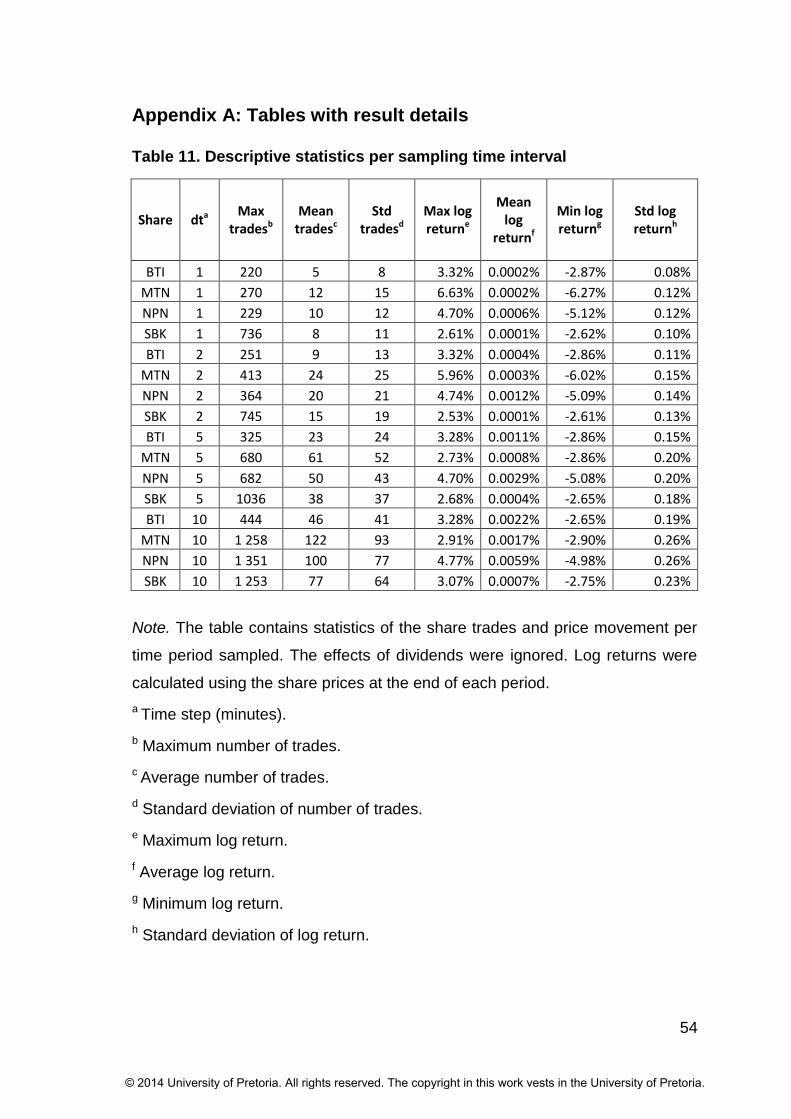
54
Appendix A: Tables with result details
Table 11. Descriptive statistics per sampling time interval
Share dta Max
tradesb Mean
tradesc Std
tradesd Max log returne
Mean log
returnf
Min log returng
Std log returnh
BTI 1 220 5 8 3.32% 0.0002% -2.87% 0.08%
MTN 1 270 12 15 6.63% 0.0002% -6.27% 0.12%
NPN 1 229 10 12 4.70% 0.0006% -5.12% 0.12%
SBK 1 736 8 11 2.61% 0.0001% -2.62% 0.10%
BTI 2 251 9 13 3.32% 0.0004% -2.86% 0.11%
MTN 2 413 24 25 5.96% 0.0003% -6.02% 0.15%
NPN 2 364 20 21 4.74% 0.0012% -5.09% 0.14%
SBK 2 745 15 19 2.53% 0.0001% -2.61% 0.13%
BTI 5 325 23 24 3.28% 0.0011% -2.86% 0.15%
MTN 5 680 61 52 2.73% 0.0008% -2.86% 0.20%
NPN 5 682 50 43 4.70% 0.0029% -5.08% 0.20%
SBK 5 1036 38 37 2.68% 0.0004% -2.65% 0.18%
BTI 10 444 46 41 3.28% 0.0022% -2.65% 0.19%
MTN 10 1 258 122 93 2.91% 0.0017% -2.90% 0.26%
NPN 10 1 351 100 77 4.77% 0.0059% -4.98% 0.26%
SBK 10 1 253 77 64 3.07% 0.0007% -2.75% 0.23%
Note. The table contains statistics of the share trades and price movement per
time period sampled. The effects of dividends were ignored. Log returns were
calculated using the share prices at the end of each period.
a Time step (minutes).
b Maximum number of trades.
c Average number of trades.
d Standard deviation of number of trades.
e Maximum log return.
f Average log return.
g Minimum log return.
h Standard deviation of log return.
© 2014 University of Pretoria. All rights reserved. The copyright in this work vests in the University of Pretoria.

55
Table 12. ARMA models fitted to log returns
Share dta ARb MAb C AR l1 AR l2 AR l3 AR l4 MA l1 MA l2 MA l3 MA l4
BTI 1 2 3 1.7E-06 0.1 0.37 0 0 -0.27 -0.41 0.05 0
BTI 2 1 1 5.1E-06 0.16 0 0 0 -0.35 0 0 0
BTI 5 1 1 1.2E-05 0.20 0 0 0 -0.34 0 0 0
BTI 10 0 1 3E-05 0 0 0 0 -0.1 0 0 0
MTN 1 0 3 4.1E-07 0 0 0 0 -0.24 -0.03 -0.03 0
MTN 2 3 0 1.1E-06 -0.21 -0.06 -0.04 0 0 0 0 0
MTN 5 0 2 2.1E-06 0 0 0 0 -0.1 -0.03 0 0
MTN 10 1 0 4.4E-06 -0.09 0 0 0 0 0 0 0
NPN 1 4 4 4.3E-06 -0.31 0.15 0.06 0.23 0.09 -0.26 -0.06 -0.23
NPN 2 0 3 10E-06 0 0 0 0 -0.2 -0.03 -0.05 0
NPN 5 0 1 2.5E-05 0 0 0 0 -0.18 0 0 0
NPN 10 0 1 5.1E-05 0 0 0 0 -0.16 0 0 0
SBK 1 1 1 -5.5E-07 0.48 0 0 0 -0.63 0 0 0
SBK 2 1 1 -1.6E-06 0.24 0 0 0 -0.44 0 0 0
SBK 5 0 1 -5.1E-06 0 0 0 0 -0.18 0 0 0
SBK 10 0 1 -1.1E-05 0 0 0 0 -0.13 0 0 0
Note. aTime step is in minutes.
bThe columns indicate the number of AR and MA lags selected for the best fit according to the BIC criterion.
The model equation is as follows:
Rt = C + AR l1 x rt-1 + AR l2 x rt-2 + AR l3 x rt-3 + AR l4 x rt-4 +
MA l1 x st-1 + MA l2 x st-2 + MA l3 x st-3 + MA l4 x st-4
With:
Rt = the predicted value of the log return at time step t.
AR l1 = the quotient of the first AR lag.
rt-1 = the actual value of the log return at time step t-1 (the previous time step)
st-1 = the value of a random input at time step t-1.
© 2014 University of Pretoria. All rights reserved. The copyright in this work vests in the University of Pretoria.

56
Table 13. Wavelet-ARMA models fitted to BTI and MTN log returns
Share BTI BTI BTI BTI MTN MTN MTN MTN
Time stepa
1 2 5 10 1 2 5 10
Scaleb 1 1 1 1 1 1 1 1
AR lagsc 2 2 2 0 1 2 1 1
MA lagsc 2 2 2 2 2 0 2 2
Constant -4E-10 -7.1E-09 -3.5E-08 5.29E-23 3.46E-09 -4.4E-09 3.81E-10 -7.5E-07
AR lag 1 -0.16 -0.103 -0.171 0 -0.160 -1.095 0.051 -0.084
AR lag 2 -0.04 0.014 -0.040 0 0 -0.522 0 0
MA lag 1 -1.45 -1.452 -1.801 -1.504 -1.520 0 -1.455 -1.823
MA lag 2 0.540 0.577 0.818 0.667 0.609 0 0.657 0.828
Scaleb 2 2 2 2 2 2 2 2
AR lagsc 2 2 2 2 2 2 2 2
MA lagsc 1 1 1 1 1 1 1 1
Constant -1E-08 -2E-08 -3.3E-08 -1.7E-07 -1.3E-08 -3.8E-09 -2.1E-08 -6.5E-08
AR lag 1 0.308 0.314 0.304 0.314 0.295 0.293 0.333 0.312
AR lag 2 -
0.725 -0.720 -0.723 -0.722 -0.744 -0.729 -0.719 -0.710
MA lag 1 0.281 0.286 0.304 0.288 0.252 0.268 0.290 0.321
MA lag 2 0 0 0 0 0 0 0 0
Scale 3 3 3 3 3 3 3 3
AR lagsc 2 2 2 2 2 2 2 2
MA lagsc 2 2 2 2 0 2 2 2
Constant -4E-09 6.32E-09 -2.9E-10 4.7E-08 1.5E-09 1.04E-10 -3E-09 -1E-08
AR lag 1 1.55 1.55 1.54 1.55 1.18 1.57 1.52 1.53
AR lag 2 -0.89 -0.892 -0.885 -0.884 -0.599 -0.894 -0.873 -0.881
MA lag 1 -0.63 -0.609 -0.557 -0.565 0.000 -0.706 -0.475 -0.464
MA lag 2 0.009 0.032 0.021 0.021 0 0.012 0.010 0.037
Scaleb 4 4 4 4 4 4 4 4
AR lagsc 2 2 2 2 2 2 2 2
MA lagsc 2 2 2 2 2 2 2 2
Constant -2E-10 -3.3E-09 3.69E-09 1.26E-08 -8.4E-10 1.82E-09 -8.5E-09 -6.6E-10
AR lag 1 1.841 1.826 1.830 1.839 1.826 1.834 1.841 1.840
AR lag 2 -0.94 -0.923 -0.923 -0.931 -0.920 -0.928 -0.933 -0.930
MA lag 1 -0.46 -0.437 -0.399 -0.352 -0.496 -0.494 -0.371 -0.367
MA lag 2 -0.13 -0.071 -0.114 -0.159 -0.084 -0.080 -0.151 -0.118
Scaleb 5 5 5 5 5 5 5 5
AR lagsc 2 2 2 2 2 2 2 2
MA lagsc 2 2 2 2 2 2 2 2
Constant -6E-10 1.35E-09 1.83E-09 -2.4E-09 -5.6E-11 3.25E-10 1.57E-09 1.21E-08
AR lag 1 1.903 1.900 1.910 1.913 1.896 1.897 1.907 1.923
AR lag 2 -0.93 -0.927 -0.937 -0.939 -0.924 -0.923 -0.933 -0.951
© 2014 University of Pretoria. All rights reserved. The copyright in this work vests in the University of Pretoria.

57
Share BTI BTI BTI BTI MTN MTN MTN MTN
Time stepa
1 2 5 10 1 2 5 10
MA lag 1 -0.27 -0.273 -0.238 -0.232 -0.345 -0.326 -0.217 -0.234
MA lag 2 -0.1 -0.077 -0.075 -0.092 -0.037 -0.029 -0.095 -0.064
Scaleb 6 6 6 6 6 6 6 6
AR lagsc 2 2 2 2 2 2 2 2
MA lagsc 2 1 2 0 2 1 0 0
Constant 4.4E-09 8.72E-09 3.32E-08 7.77E-08 4.11E-09 8.66E-09 1.87E-08 3.15E-08
AR lag 1 1.943 1.946 1.953 1.947 1.947 1.950 1.942 1.938
AR lag 2 -0.95 -0.949 -0.956 -0.950 -0.950 -0.953 -0.946 -0.941
MA lag 1 -0.17 -0.167 -0.155 0 -0.277 -0.242 0 0
MA lag 2 -0.04 0 -0.034 0 -0.026 0 0 0
Note. aTime step is in minutes.
bThe lowest scale number designates the highest frequency component. For instance, in the case of the 1 minute time step, scale 1 refers to the cycles of duration 1 to 2 minutes.
cThe rows indicate the number of AR and MA lags selected for the best fit according to the BIC criterion.
The model equation is as follows:
Rst = Constant + ARlag1 x rs
t-1 + ARlag2 x rst-2 + MAlag1 x ss
t-1 + MAlag2 x sst-2 .
With:
Rst = the predicted value of the relevant scale component log return at time step
t.
Rst-1 = the actual value of the scale component of the log return at time step t-1
(the previous time step)
Sst-1 = the value of a random input at time step t-1.
The predicted return at time step t is the sum of the selected scale component predicted values. For instance, in the case of the wavelet-ARMA scale 3-6 algorithm,
Rt = R3t + R4
t + R5t + R6
t.
© 2014 University of Pretoria. All rights reserved. The copyright in this work vests in the University of Pretoria.

58
Table 14. Wavelet-ARMA models fitted to NPN and SBK log returns
Share NPN NPN NPN NPN SBK SBK SBK SBK
Time stepa
1 2 5 10 1 2 5 10
Scaleb 1 1 1 1 1 1 1 1
AR lagsc 1 2 2 2 1 1 2 2
MA lagsc 2 0 2 2 2 2 2 2
Constant 1.4E-09 -3.3E-08 1.35E-07 3.03E-
08 2.39E-10 5.19E-10 -1.4E-09 -3.1E-07
AR lag 1 -0.060 -1.088 -0.250 -0.147 -0.004 -0.040 -0.252 -0.150
AR lag 2 0 -0.536 -0.059 -0.010 0 0 -0.054 -0.115
MA lag 1 -1.507 0 -1.894 -1.428 -1.506 -1.387 -1.356 -1.921
MA lag 2 0.668 0 0.900 0.541 0.636 0.651 0.434 0.926
Scaleb 2 2 2 2 2 2 2 2
AR lagsc 2 2 2 2 2 2 2 2
MA lagsc 1 1 1 1 1 1 1 1
Constant 7.5E-09 1.26E-08 2.55E-08 -6.7E-08 -2.7E-09 5.75E-09 4.29E-08 -1.1E-07
AR lag 1 0.297 0.283 0.290 0.318 0.338 0.310 0.346 0.343
AR lag 2 -0.733 -0.722 -0.717 -0.721 -0.732 -0.727 -0.715 -0.728
MA lag 1 0.254 0.277 0.284 0.279 0.263 0.270 0.252 0.248
MA lag 2 0 0 0 0 0 0 0 0
Scale 3 3 3 3 3 3 3 3
AR lagsc 2 2 2 2 2 2 2 2
MA lagsc 1 2 1 2 1 2 1 2
Constant 2.4E-09 1.91E-08 -1E-08 2.76E-
08 -6.7E-09 3.23E-09 -6.8E-09 -9E-08
AR lag 1 1.566 1.565 1.572 1.561 1.535 1.566 1.556 1.547
AR lag 2 -0.893 -0.895 -0.896 -0.891 -0.885 -0.891 -0.893 -0.877
MA lag 1 -0.738 -0.707 -0.691 -0.628 -0.566 -0.685 -0.649 -0.564
MA lag 2 0 0.024 0 0.024 0 0.005 0 0.017
Scaleb 4 4 4 4 4 4 4 4
AR lagsc 2 2 2 2 2 2 2 2
MA lagsc 2 2 2 2 2 2 2 2
Constant 3.2E-09 2.5E-09 3.31E-09 -5.8E-09 -1.2E-09 -4.6E-09 -1E-08 -2.3E-08
AR lag 1 1.839 1.847 1.849 1.827 1.837 1.824 1.826 1.854
AR lag 2 -0.931 -0.938 -0.939 -0.923 -0.928 -0.923 -0.918 -0.945
MA lag 1 -0.494 -0.524 -0.467 -0.403 -0.414 -0.440 -0.409 -0.400
MA lag 2 -0.143 -0.110 -0.130 -0.112 -0.195 -0.094 -0.118 -0.219
Scaleb 5 5 5 5 5 5 5 5
AR lagsc 2 2 2 2 2 2 2 2
MA lagsc 2 2 2 2 2 2 2 2
Constant 6.5E-10 1.09E-09 7.48E-10 -2.9E-10 -1E-09 -2.2E-09 -1.1E-09 -6.8E-09
AR lag 1 1.908 1.902 1.904 1.907 1.898 1.893 1.898 1.885
AR lag 2 -0.935 -0.929 -0.932 -0.932 -0.927 -0.921 -0.926 -0.914
© 2014 University of Pretoria. All rights reserved. The copyright in this work vests in the University of Pretoria.
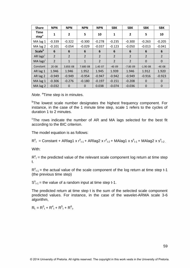
59
Share NPN NPN NPN NPN SBK SBK SBK SBK
Time stepa
1 2 5 10 1 2 5 10
MA lag 1 -0.339 -0.322 -0.300 -0.278 -0.235 -0.300 -0.263 -0.205
MA lag 2 -0.101 -0.054 -0.029 -0.037 -0.123 -0.050 -0.013 -0.041
Scaleb 6 6 6 6 6 6 6 6
AR lagsc 2 2 2 2 2 2 2 2
MA lagsc 2 1 1 2 2 2 0 0
Constant 2E-08 3.85E-08 7.68E-08 1.4E-07 -4E-09 -7.8E-09 -1.9E-08 -4E-08
AR lag 1 1.946 1.946 1.952 1.945 1.939 1.946 1.912 1.920
AR lag 2 -0.949 -0.949 -0.954 -0.947 -0.942 -0.949 -0.916 -0.923
MA lag 1 -0.306 -0.276 -0.180 -0.197 -0.151 -0.208 0 0
MA lag 2 -0.032 0 0 0.038 -0.074 -0.036 0 0
Note. aTime step is in minutes.
bThe lowest scale number designates the highest frequency component. For instance, in the case of the 1 minute time step, scale 1 refers to the cycles of duration 1 to 2 minutes.
cThe rows indicate the number of AR and MA lags selected for the best fit according to the BIC criterion.
The model equation is as follows:
Rst = Constant + ARlag1 x rs
t-1 + ARlag2 x rst-2 + MAlag1 x ss
t-1 + MAlag2 x sst-2 .
With:
Rst = the predicted value of the relevant scale component log return at time step
t.
Rst-1 = the actual value of the scale component of the log return at time step t-1
(the previous time step)
Sst-1 = the value of a random input at time step t-1.
The predicted return at time step t is the sum of the selected scale component predicted values. For instance, in the case of the wavelet-ARMA scale 3-6 algorithm,
Rt = R3t + R4
t + R5t + R6
t.
© 2014 University of Pretoria. All rights reserved. The copyright in this work vests in the University of Pretoria.
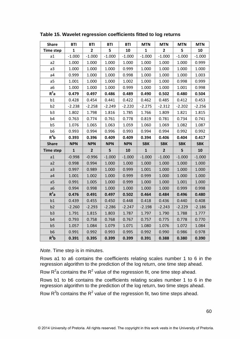
60
Table 15. Wavelet regression coefficients fitted to log returns
Share BTI BTI BTI BTI MTN MTN MTN MTN
Time step 1 2 5 10 1 2 5 10
a1 -1.000 -1.000 -1.000 -1.000 -1.000 -1.000 -1.000 -1.000
a2 1.000 1.000 1.000 1.000 1.000 1.000 1.000 0.999
a3 1.000 1.000 1.000 0.999 1.000 1.000 1.000 1.000
a4 0.999 1.000 1.000 0.998 1.000 1.000 1.000 1.003
a5 1.001 1.000 1.000 1.002 1.000 1.000 0.998 0.999
a6 1.000 1.000 1.000 0.999 1.000 1.000 1.001 0.998
R2a 0.479 0.497 0.486 0.489 0.490 0.502 0.480 0.504
b1 0.428 0.454 0.441 0.422 0.462 0.485 0.412 0.453
b2 -2.238 -2.258 -2.249 -2.220 -2.275 -2.312 -2.202 -2.256
b3 1.802 1.798 1.816 1.785 1.766 1.809 1.821 1.815
b4 0.763 0.774 0.761 0.778 0.819 0.781 0.734 0.741
b5 1.076 1.065 1.063 1.059 1.060 1.069 1.082 1.087
b6 0.993 0.994 0.996 0.993 0.994 0.994 0.992 0.992
R2b 0.393 0.396 0.409 0.409 0.394 0.406 0.404 0.417
Share NPN NPN NPN NPN SBK SBK SBK SBK
Time step 1 2 5 10 1 2 5 10
a1 -0.998 -0.996 -1.000 -1.000 -1.000 -1.000 -1.000 -1.000
a2 0.998 0.994 1.000 1.000 1.000 1.000 1.000 1.000
a3 0.997 0.989 1.000 0.999 1.001 1.000 1.000 1.000
a4 1.001 1.002 1.000 0.999 0.999 1.000 1.000 1.000
a5 0.991 1.005 1.000 0.999 1.000 1.000 1.001 1.000
a6 0.994 0.998 1.000 1.000 1.000 1.000 0.999 0.998
R2a 0.476 0.491 0.497 0.502 0.464 0.484 0.496 0.480
b1 0.439 0.455 0.450 0.448 0.418 0.436 0.440 0.408
b2 -2.260 -2.293 -2.286 -2.247 -2.198 -2.243 -2.229 -2.186
b3 1.791 1.815 1.803 1.787 1.797 1.790 1.788 1.777
b4 0.793 0.758 0.768 0.767 0.757 0.775 0.778 0.770
b5 1.057 1.084 1.079 1.071 1.080 1.076 1.072 1.084
b6 0.991 0.992 0.993 0.995 0.992 0.990 0.986 0.978
R2b 0.391 0.395 0.399 0.399 0.391 0.388 0.380 0.390
Note. Time step is in minutes.
Rows a1 to a6 contains the coefficients relating scales number 1 to 6 in the regression algorithm to the prediction of the log return, one time step ahead.
Row R2a contains the R2 value of the regression fit, one time step ahead.
Rows b1 to b6 contains the coefficients relating scales number 1 to 6 in the regression algorithm to the prediction of the log return, two time steps ahead.
Row R2b contains the R2 value of the regression fit, two time steps ahead.
© 2014 University of Pretoria. All rights reserved. The copyright in this work vests in the University of Pretoria.
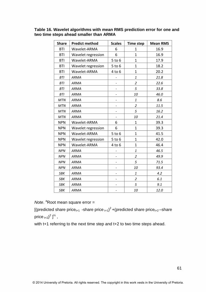
61
Table 16. Wavelet algorithms with mean RMS prediction error for one and two time steps ahead smaller than ARMA
Share Predict method Scales Time step Mean RMS
BTI Wavelet-ARMA 6 1 16.9
BTI Wavelet regression 6 1 16.9
BTI Wavelet-ARMA 5 to 6 1 17.9
BTI Wavelet regression 5 to 6 1 18.2
BTI Wavelet-ARMA 4 to 6 1 20.2
BTI ARMA - 1 21.8
BTI ARMA - 2 22.6
BTI ARMA - 5 33.8
BTI ARMA - 10 46.0
MTN ARMA - 1 8.6
MTN ARMA - 2 11.5
MTN ARMA - 5 16.2
MTN ARMA - 10 21.4
NPN Wavelet-ARMA 6 1 39.3
NPN Wavelet regression 6 1 39.3
NPN Wavelet-ARMA 5 to 6 1 41.5
NPN Wavelet regression 5 to 6 1 42.0
NPN Wavelet-ARMA 4 to 6 1 46.4
NPN ARMA - 1 46.5
NPN ARMA - 2 49.9
NPN ARMA - 5 71.5
NPN ARMA - 10 93.4
SBK ARMA - 1 4.2
SBK ARMA - 2 6.1
SBK ARMA - 5 9.1
SBK ARMA - 10 12.0
Note. aRoot mean square error =
[(predicted share pricet+1 -share price t+1)2 +(predicted share pricet+2 –share
price t+2)2 ]½ ,
with t+1 referring to the next time step and t+2 to two time steps ahead.
© 2014 University of Pretoria. All rights reserved. The copyright in this work vests in the University of Pretoria.

62
Table 17. Wavelet algorithms predicting the price change direction of the next two steps better than ARMA
Share Predict method Scales Time step
Dir1 % right
Dir2 % right
Dir Both
% right
BTI Wavelet regression 2 to 6 1 33.3% 27.2% 17.6%
MTN Wavelet regression 2 to 6 1 36.7% 32.6% 25.3%
NPN Wavelet regression 2 to 6 1 37.0% 32.9% 25.5%
SBK Wavelet regression 2 to 6 1 33.8% 27.6% 17.9%
BTI Wavelet-ARMA 2 to 6 1 30.4% 25.0% 15.3%
MTN Wavelet-ARMA 2 to 6 1 33.7% 30.3% 22.9%
NPN Wavelet-ARMA 2 to 6 1 33.5% 30.2% 22.6%
SBK Wavelet-ARMA 2 to 6 1 30.9% 25.6% 15.6%
BTI Wavelet-ARMA 3 to 6 1 27.8% 22.9% 13.3%
MTN Wavelet-ARMA 3 to 6 1 31.3% 27.8% 20.6%
NPN Wavelet-ARMA 3 to 6 1 29.6% 26.6% 19.1%
SBK Wavelet-ARMA 3 to 6 1 28.3% 23.6% 13.7%
BTI Wavelet regression 3 to 6 1 27.0% 22.1% 12.7%
MTN Wavelet regression 3 to 6 1 30.4% 27.3% 20.1%
NPN Wavelet regression 3 to 6 1 28.6% 25.3% 18.2%
SBK Wavelet regression 3 to 6 1 27.6% 22.6% 13.3%
BTI ARMA - 1 26.2% 21.4% 12.2%
MTN Wavelet-ARMA 4 to 6 1 28.1% 25.5% 18.5%
NPN Wavelet-ARMA 4 to 6 1 26.6% 24.1% 17.0%
SBK Wavelet-ARMA 4 to 6 1 25.2% 21.3% 12.0%
MTN Wavelet regression 4 to 6 1 27.6% 25.2% 18.3%
NPN Wavelet regression 4 to 6 1 26.0% 23.4% 16.5%
SBK Wavelet regression 4 to 6 1 24.7% 21.1% 11.9%
NPN Wavelet-ARMA 5 to 6 1 25.0% 22.9% 16.0%
MTN Wavelet regression 5 to 6 1 26.0% 24.2% 17.2%
NPN Wavelet regression 5 to 6 1 24.6% 22.6% 15.7%
SBK Wavelet regression 5 to 6 1 23.1% 20.3% 11.1%
MTN Wavelet-ARMA 5 to 6 1 26.0% 24.1% 17.2%
SBK Wavelet-ARMA 5 to 6 1 23.2% 20.1% 11.0%
MTN Wavelet-ARMA 6 1 24.3% 22.8% 16.0%
MTN Wavelet regression 6 1 24.2% 22.8% 15.9%
NPN Wavelet regression 6 1 23.2% 22.0% 15.0%
SBK Wavelet regression 6 1 21.3% 19.4% 10.1%
NPN Wavelet-ARMA 6 1 23.2% 22.0% 15.0%
SBK Wavelet-ARMA 6 1 21.3% 19.4% 10.1%
MTN Wavelet-ARMA 1 to 6 1 20.9% 20.9% 13.9%
NPN Wavelet-ARMA 1 to 6 1 20.0% 20.6% 13.4%
© 2014 University of Pretoria. All rights reserved. The copyright in this work vests in the University of Pretoria.
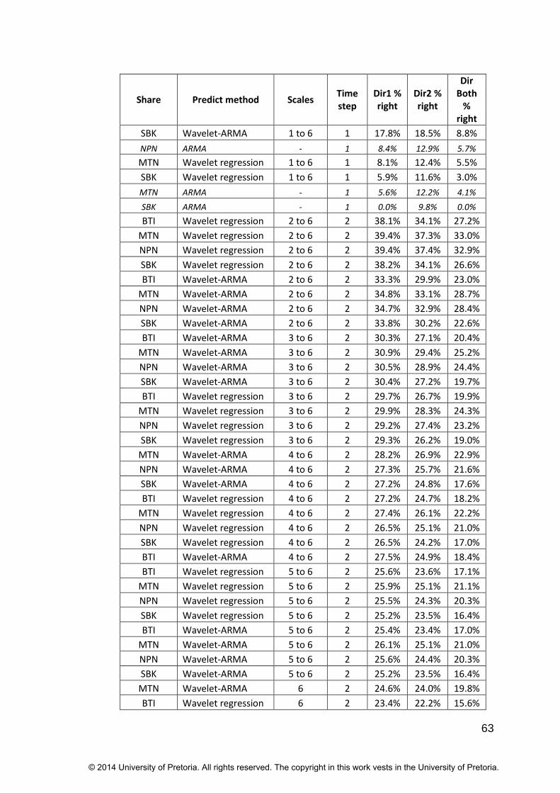
63
Share Predict method Scales Time step
Dir1 % right
Dir2 % right
Dir Both
% right
SBK Wavelet-ARMA 1 to 6 1 17.8% 18.5% 8.8%
NPN ARMA - 1 8.4% 12.9% 5.7%
MTN Wavelet regression 1 to 6 1 8.1% 12.4% 5.5%
SBK Wavelet regression 1 to 6 1 5.9% 11.6% 3.0%
MTN ARMA - 1 5.6% 12.2% 4.1%
SBK ARMA - 1 0.0% 9.8% 0.0%
BTI Wavelet regression 2 to 6 2 38.1% 34.1% 27.2%
MTN Wavelet regression 2 to 6 2 39.4% 37.3% 33.0%
NPN Wavelet regression 2 to 6 2 39.4% 37.4% 32.9%
SBK Wavelet regression 2 to 6 2 38.2% 34.1% 26.6%
BTI Wavelet-ARMA 2 to 6 2 33.3% 29.9% 23.0%
MTN Wavelet-ARMA 2 to 6 2 34.8% 33.1% 28.7%
NPN Wavelet-ARMA 2 to 6 2 34.7% 32.9% 28.4%
SBK Wavelet-ARMA 2 to 6 2 33.8% 30.2% 22.6%
BTI Wavelet-ARMA 3 to 6 2 30.3% 27.1% 20.4%
MTN Wavelet-ARMA 3 to 6 2 30.9% 29.4% 25.2%
NPN Wavelet-ARMA 3 to 6 2 30.5% 28.9% 24.4%
SBK Wavelet-ARMA 3 to 6 2 30.4% 27.2% 19.7%
BTI Wavelet regression 3 to 6 2 29.7% 26.7% 19.9%
MTN Wavelet regression 3 to 6 2 29.9% 28.3% 24.3%
NPN Wavelet regression 3 to 6 2 29.2% 27.4% 23.2%
SBK Wavelet regression 3 to 6 2 29.3% 26.2% 19.0%
MTN Wavelet-ARMA 4 to 6 2 28.2% 26.9% 22.9%
NPN Wavelet-ARMA 4 to 6 2 27.3% 25.7% 21.6%
SBK Wavelet-ARMA 4 to 6 2 27.2% 24.8% 17.6%
BTI Wavelet regression 4 to 6 2 27.2% 24.7% 18.2%
MTN Wavelet regression 4 to 6 2 27.4% 26.1% 22.2%
NPN Wavelet regression 4 to 6 2 26.5% 25.1% 21.0%
SBK Wavelet regression 4 to 6 2 26.5% 24.2% 17.0%
BTI Wavelet-ARMA 4 to 6 2 27.5% 24.9% 18.4%
BTI Wavelet regression 5 to 6 2 25.6% 23.6% 17.1%
MTN Wavelet regression 5 to 6 2 25.9% 25.1% 21.1%
NPN Wavelet regression 5 to 6 2 25.5% 24.3% 20.3%
SBK Wavelet regression 5 to 6 2 25.2% 23.5% 16.4%
BTI Wavelet-ARMA 5 to 6 2 25.4% 23.4% 17.0%
MTN Wavelet-ARMA 5 to 6 2 26.1% 25.1% 21.0%
NPN Wavelet-ARMA 5 to 6 2 25.6% 24.4% 20.3%
SBK Wavelet-ARMA 5 to 6 2 25.2% 23.5% 16.4%
MTN Wavelet-ARMA 6 2 24.6% 24.0% 19.8%
BTI Wavelet regression 6 2 23.4% 22.2% 15.6%
© 2014 University of Pretoria. All rights reserved. The copyright in this work vests in the University of Pretoria.

64
Share Predict method Scales Time step
Dir1 % right
Dir2 % right
Dir Both
% right
MTN Wavelet regression 6 2 24.5% 23.9% 19.7%
NPN Wavelet regression 6 2 24.1% 23.4% 19.2%
SBK Wavelet regression 6 2 23.5% 22.2% 15.2%
BTI Wavelet-ARMA 6 2 23.5% 22.2% 15.6%
NPN Wavelet-ARMA 6 2 24.1% 23.5% 19.2%
SBK Wavelet-ARMA 6 2 23.4% 22.2% 15.1%
BTI Wavelet-ARMA 1 to 6 2 20.5% 20.8% 14.1%
MTN Wavelet-ARMA 1 to 6 2 19.0% 19.7% 15.4%
NPN Wavelet-ARMA 1 to 6 2 19.1% 19.6% 15.3%
SBK Wavelet-ARMA 1 to 6 2 19.7% 20.3% 13.0%
BTI Wavelet regression 1 to 6 2 8.2% 12.6% 5.9%
MTN Wavelet regression 1 to 6 2 9.4% 12.3% 7.8%
NPN Wavelet regression 1 to 6 2 9.2% 12.0% 7.3%
SBK Wavelet regression 1 to 6 2 7.7% 12.5% 5.2%
BTI ARMA - 2 4.8% 10.9% 3.5%
MTN ARMA - 2 5.5% 8.9% 4.5%
NPN ARMA - 2 8.5% 12.0% 6.9%
SBK ARMA - 2 4.7% 11.3% 3.3%
BTI Wavelet regression 2 to 6 5 39.1% 38.0% 35.3%
MTN Wavelet regression 2 to 6 5 40.7% 39.9% 38.0%
SBK Wavelet regression 2 to 6 5 41.1% 39.5% 36.1%
NPN Wavelet-ARMA 1 to 6 5 49.8% 48.5% 46.9%
NPN Wavelet regression 2 to 6 5 41.6% 40.9% 39.3%
BTI Wavelet-ARMA 2 to 6 5 35.6% 34.5% 31.9%
MTN Wavelet-ARMA 2 to 6 5 34.2% 33.8% 31.8%
SBK Wavelet-ARMA 2 to 6 5 35.3% 33.9% 30.2%
NPN Wavelet-ARMA 2 to 6 5 34.3% 33.8% 32.1%
BTI Wavelet-ARMA 3 to 6 5 32.2% 31.1% 28.6%
MTN Wavelet-ARMA 3 to 6 5 30.2% 29.8% 27.8%
SBK Wavelet-ARMA 3 to 6 5 30.2% 29.1% 25.5%
BTI Wavelet regression 3 to 6 5 31.5% 30.6% 27.9%
MTN Wavelet regression 3 to 6 5 28.6% 28.1% 26.2%
SBK Wavelet regression 3 to 6 5 28.9% 27.9% 24.3%
NPN Wavelet-ARMA 3 to 6 5 29.4% 28.8% 27.4%
NPN Wavelet regression 3 to 6 5 28.1% 27.6% 26.1%
MTN Wavelet-ARMA 4 to 6 5 27.6% 27.4% 25.4%
SBK Wavelet-ARMA 4 to 6 5 28.2% 27.3% 23.7%
BTI Wavelet regression 4 to 6 5 29.1% 28.2% 25.8%
MTN Wavelet regression 4 to 6 5 26.5% 26.3% 24.3%
SBK Wavelet regression 4 to 6 5 27.0% 26.2% 22.7%
© 2014 University of Pretoria. All rights reserved. The copyright in this work vests in the University of Pretoria.
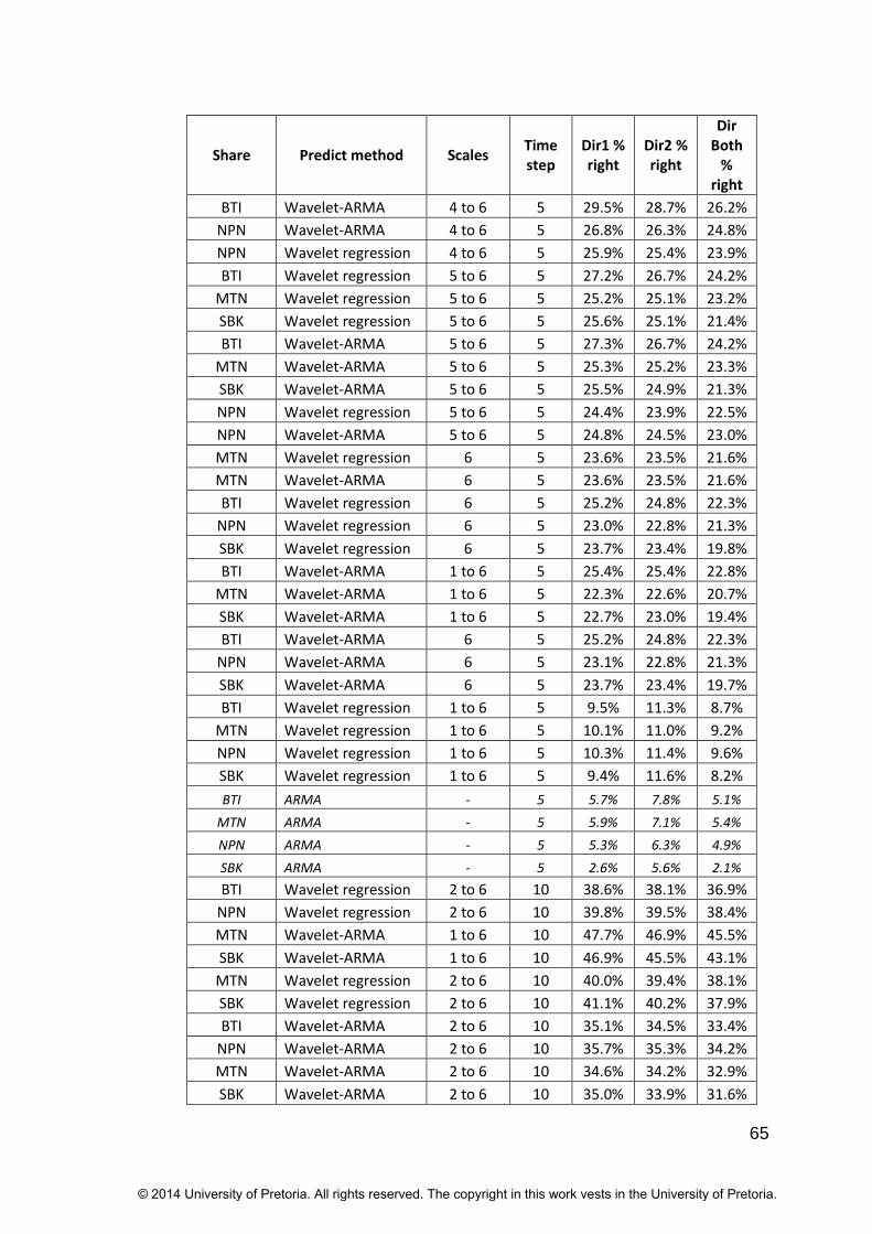
65
Share Predict method Scales Time step
Dir1 % right
Dir2 % right
Dir Both
% right
BTI Wavelet-ARMA 4 to 6 5 29.5% 28.7% 26.2%
NPN Wavelet-ARMA 4 to 6 5 26.8% 26.3% 24.8%
NPN Wavelet regression 4 to 6 5 25.9% 25.4% 23.9%
BTI Wavelet regression 5 to 6 5 27.2% 26.7% 24.2%
MTN Wavelet regression 5 to 6 5 25.2% 25.1% 23.2%
SBK Wavelet regression 5 to 6 5 25.6% 25.1% 21.4%
BTI Wavelet-ARMA 5 to 6 5 27.3% 26.7% 24.2%
MTN Wavelet-ARMA 5 to 6 5 25.3% 25.2% 23.3%
SBK Wavelet-ARMA 5 to 6 5 25.5% 24.9% 21.3%
NPN Wavelet regression 5 to 6 5 24.4% 23.9% 22.5%
NPN Wavelet-ARMA 5 to 6 5 24.8% 24.5% 23.0%
MTN Wavelet regression 6 5 23.6% 23.5% 21.6%
MTN Wavelet-ARMA 6 5 23.6% 23.5% 21.6%
BTI Wavelet regression 6 5 25.2% 24.8% 22.3%
NPN Wavelet regression 6 5 23.0% 22.8% 21.3%
SBK Wavelet regression 6 5 23.7% 23.4% 19.8%
BTI Wavelet-ARMA 1 to 6 5 25.4% 25.4% 22.8%
MTN Wavelet-ARMA 1 to 6 5 22.3% 22.6% 20.7%
SBK Wavelet-ARMA 1 to 6 5 22.7% 23.0% 19.4%
BTI Wavelet-ARMA 6 5 25.2% 24.8% 22.3%
NPN Wavelet-ARMA 6 5 23.1% 22.8% 21.3%
SBK Wavelet-ARMA 6 5 23.7% 23.4% 19.7%
BTI Wavelet regression 1 to 6 5 9.5% 11.3% 8.7%
MTN Wavelet regression 1 to 6 5 10.1% 11.0% 9.2%
NPN Wavelet regression 1 to 6 5 10.3% 11.4% 9.6%
SBK Wavelet regression 1 to 6 5 9.4% 11.6% 8.2%
BTI ARMA - 5 5.7% 7.8% 5.1%
MTN ARMA - 5 5.9% 7.1% 5.4%
NPN ARMA - 5 5.3% 6.3% 4.9%
SBK ARMA - 5 2.6% 5.6% 2.1%
BTI Wavelet regression 2 to 6 10 38.6% 38.1% 36.9%
NPN Wavelet regression 2 to 6 10 39.8% 39.5% 38.4%
MTN Wavelet-ARMA 1 to 6 10 47.7% 46.9% 45.5%
SBK Wavelet-ARMA 1 to 6 10 46.9% 45.5% 43.1%
MTN Wavelet regression 2 to 6 10 40.0% 39.4% 38.1%
SBK Wavelet regression 2 to 6 10 41.1% 40.2% 37.9%
BTI Wavelet-ARMA 2 to 6 10 35.1% 34.5% 33.4%
NPN Wavelet-ARMA 2 to 6 10 35.7% 35.3% 34.2%
MTN Wavelet-ARMA 2 to 6 10 34.6% 34.2% 32.9%
SBK Wavelet-ARMA 2 to 6 10 35.0% 33.9% 31.6%
© 2014 University of Pretoria. All rights reserved. The copyright in this work vests in the University of Pretoria.
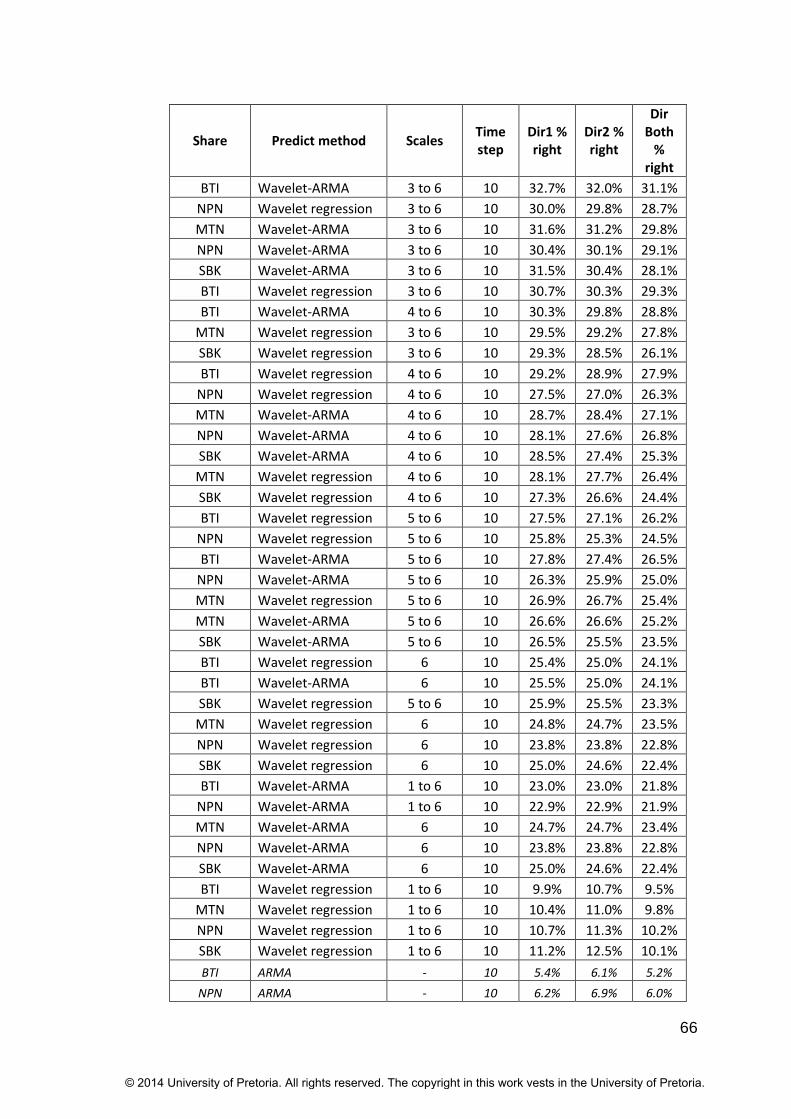
66
Share Predict method Scales Time step
Dir1 % right
Dir2 % right
Dir Both
% right
BTI Wavelet-ARMA 3 to 6 10 32.7% 32.0% 31.1%
NPN Wavelet regression 3 to 6 10 30.0% 29.8% 28.7%
MTN Wavelet-ARMA 3 to 6 10 31.6% 31.2% 29.8%
NPN Wavelet-ARMA 3 to 6 10 30.4% 30.1% 29.1%
SBK Wavelet-ARMA 3 to 6 10 31.5% 30.4% 28.1%
BTI Wavelet regression 3 to 6 10 30.7% 30.3% 29.3%
BTI Wavelet-ARMA 4 to 6 10 30.3% 29.8% 28.8%
MTN Wavelet regression 3 to 6 10 29.5% 29.2% 27.8%
SBK Wavelet regression 3 to 6 10 29.3% 28.5% 26.1%
BTI Wavelet regression 4 to 6 10 29.2% 28.9% 27.9%
NPN Wavelet regression 4 to 6 10 27.5% 27.0% 26.3%
MTN Wavelet-ARMA 4 to 6 10 28.7% 28.4% 27.1%
NPN Wavelet-ARMA 4 to 6 10 28.1% 27.6% 26.8%
SBK Wavelet-ARMA 4 to 6 10 28.5% 27.4% 25.3%
MTN Wavelet regression 4 to 6 10 28.1% 27.7% 26.4%
SBK Wavelet regression 4 to 6 10 27.3% 26.6% 24.4%
BTI Wavelet regression 5 to 6 10 27.5% 27.1% 26.2%
NPN Wavelet regression 5 to 6 10 25.8% 25.3% 24.5%
BTI Wavelet-ARMA 5 to 6 10 27.8% 27.4% 26.5%
NPN Wavelet-ARMA 5 to 6 10 26.3% 25.9% 25.0%
MTN Wavelet regression 5 to 6 10 26.9% 26.7% 25.4%
MTN Wavelet-ARMA 5 to 6 10 26.6% 26.6% 25.2%
SBK Wavelet-ARMA 5 to 6 10 26.5% 25.5% 23.5%
BTI Wavelet regression 6 10 25.4% 25.0% 24.1%
BTI Wavelet-ARMA 6 10 25.5% 25.0% 24.1%
SBK Wavelet regression 5 to 6 10 25.9% 25.5% 23.3%
MTN Wavelet regression 6 10 24.8% 24.7% 23.5%
NPN Wavelet regression 6 10 23.8% 23.8% 22.8%
SBK Wavelet regression 6 10 25.0% 24.6% 22.4%
BTI Wavelet-ARMA 1 to 6 10 23.0% 23.0% 21.8%
NPN Wavelet-ARMA 1 to 6 10 22.9% 22.9% 21.9%
MTN Wavelet-ARMA 6 10 24.7% 24.7% 23.4%
NPN Wavelet-ARMA 6 10 23.8% 23.8% 22.8%
SBK Wavelet-ARMA 6 10 25.0% 24.6% 22.4%
BTI Wavelet regression 1 to 6 10 9.9% 10.7% 9.5%
MTN Wavelet regression 1 to 6 10 10.4% 11.0% 9.8%
NPN Wavelet regression 1 to 6 10 10.7% 11.3% 10.2%
SBK Wavelet regression 1 to 6 10 11.2% 12.5% 10.1%
BTI ARMA - 10 5.4% 6.1% 5.2%
NPN ARMA - 10 6.2% 6.9% 6.0%
© 2014 University of Pretoria. All rights reserved. The copyright in this work vests in the University of Pretoria.
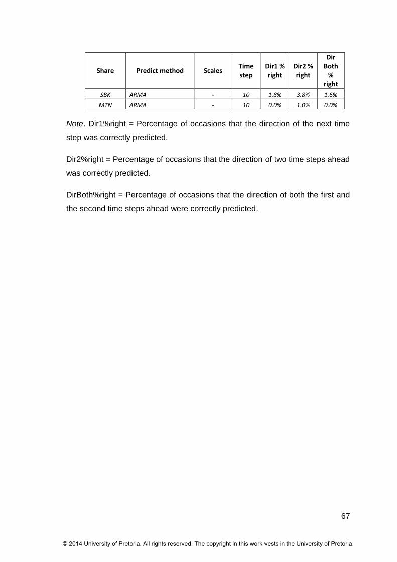
67
Share Predict method Scales Time step
Dir1 % right
Dir2 % right
Dir Both
% right
SBK ARMA - 10 1.8% 3.8% 1.6%
MTN ARMA - 10 0.0% 1.0% 0.0%
Note. Dir1%right = Percentage of occasions that the direction of the next time
step was correctly predicted.
Dir2%right = Percentage of occasions that the direction of two time steps ahead
was correctly predicted.
DirBoth%right = Percentage of occasions that the direction of both the first and
the second time steps ahead were correctly predicted.
© 2014 University of Pretoria. All rights reserved. The copyright in this work vests in the University of Pretoria.

68
Table 18. Shares with predicting and trading methods better than ARMA, buy-and-sell at time steps 1,2,5 and 10 minutes
Time step (minutes)
Method 1 2 5 10
Buy and hold BTI NPN NPN NPN NPN
Wavelet-ARMA 5-6 Short & Close BTI NPN SBK BTI NPN SBK
Wavelet-ARMA 6 Short & Close BTI NPN SBK NPN
Wavelet regression 6 Short & Close BTI NPN SBK NPN
Wavelet regression 5-6 Short & Close BTI
Wavelet-ARMA 4-6 Short & Close BTI
© 2014 University of Pretoria. All rights reserved. The copyright in this work vests in the University of Pretoria.

69
Table 19. Algorithms and trade methods with positive cumulative returns
Time step (minutes) + / # tradesb
Share Predict method Scales Tradea 1 2 5 10
BTI Wavelet-ARMA 5 to 6 S&C 12.35% 72/144
BTI Wavelet-ARMA 5 to 6 S&C 9.51% 76/152
BTI None - B&H 8.57%
BTI Wavelet-ARMA 4 to 6 S&C 7.63% 230/518
BTI Wavelet-ARMA 6 S&C 6.80% 18/26
BTI Wavelet regression 6 S&C 6.80% 18/26
BTI Wavelet regression 5 to 6 S&C 5.68% 96/205
BTI ARMA - B&S 1.7% 3/7
BTI ARMA - B&S 0.06% 3/9
MTN None - B&H 17.58%
MTN ARMA - B&S 3.04% 12/25
MTN ARMA - B&S 0.8% 7/10
MTN ARMA - B&S 0.10% 14/38
NPN None - B&H 39.84%
NPN Wavelet regression 6 S&C 11.8% 39/69
NPN Wavelet-ARMA 6 S&C 10.9% 39/68
NPN Wavelet-ARMA 5 to 6 S&C 3.3% 100/181
NPN Wavelet regression 6 S&C 2.78% 41/82
NPN Wavelet-ARMA 6 S&C 2.62% 41/82
NPN ARMA - B&S 2.04% 20/46
NPN Wavelet-ARMA 5 to 6 S&C 1.42% 141/281
SBK Wavelet-ARMA 5 to 6 S&C 18.34% 121/217
SBK None - B&H 15.83%
SBK Wavelet-ARMA 5 to 6 S&C 8.5% 102/174
SBK Wavelet regression 6 S&C 3.41% 13/43
SBK Wavelet-ARMA 6 S&C 0.48% 27/43
Note. The percentages are the cumulative returns during the test period.
a Trade method. B&H=buy and hold; B&S = buy and sell; S&C= Short and close.
b The number of profitable trades/number of trades through the 125 days period.
© 2014 University of Pretoria. All rights reserved. The copyright in this work vests in the University of Pretoria.
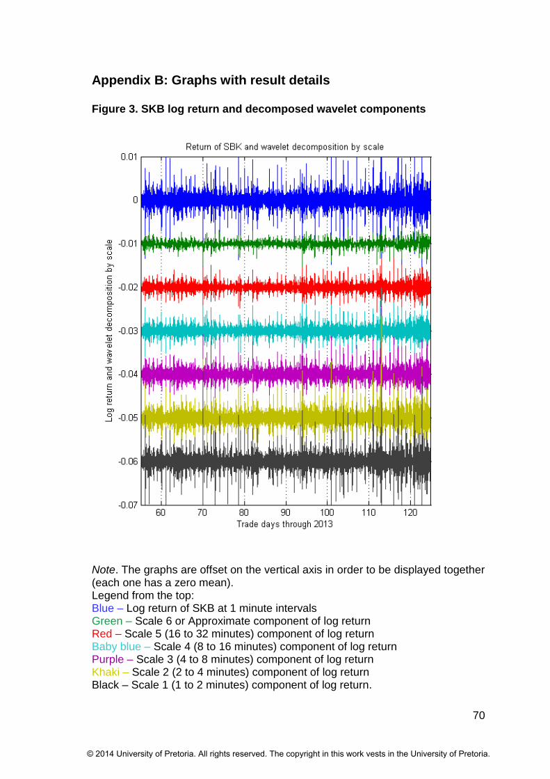
70
Appendix B: Graphs with result details
Figure 3. SKB log return and decomposed wavelet components
Note. The graphs are offset on the vertical axis in order to be displayed together (each one has a zero mean). Legend from the top: Blue – Log return of SKB at 1 minute intervals Green – Scale 6 or Approximate component of log return Red – Scale 5 (16 to 32 minutes) component of log return Baby blue – Scale 4 (8 to 16 minutes) component of log return Purple – Scale 3 (4 to 8 minutes) component of log return Khaki – Scale 2 (2 to 4 minutes) component of log return Black – Scale 1 (1 to 2 minutes) component of log return.
© 2014 University of Pretoria. All rights reserved. The copyright in this work vests in the University of Pretoria.

71
Figure 4. SKB log return and decomposed wavelet components – 12 days
Note. The graphs are offset on the vertical axis in order to be displayed together (each one has a zero mean). Legend from the top: Blue – Log return of SKB at 1 minute intervals Green – Scale 6 or approximate component of log return Red – Scale 5 (16 to 32 minutes) component of log return Baby blue – Scale 4 (8 to 16 minutes) component of log return Purple – Scale 3 (4 to 8 minutes) component of log return Khaki – Scale 2 (2 to 4 minutes) component of log return Black – Scale 1 (1 to 2 minutes) component of log return.
© 2014 University of Pretoria. All rights reserved. The copyright in this work vests in the University of Pretoria.
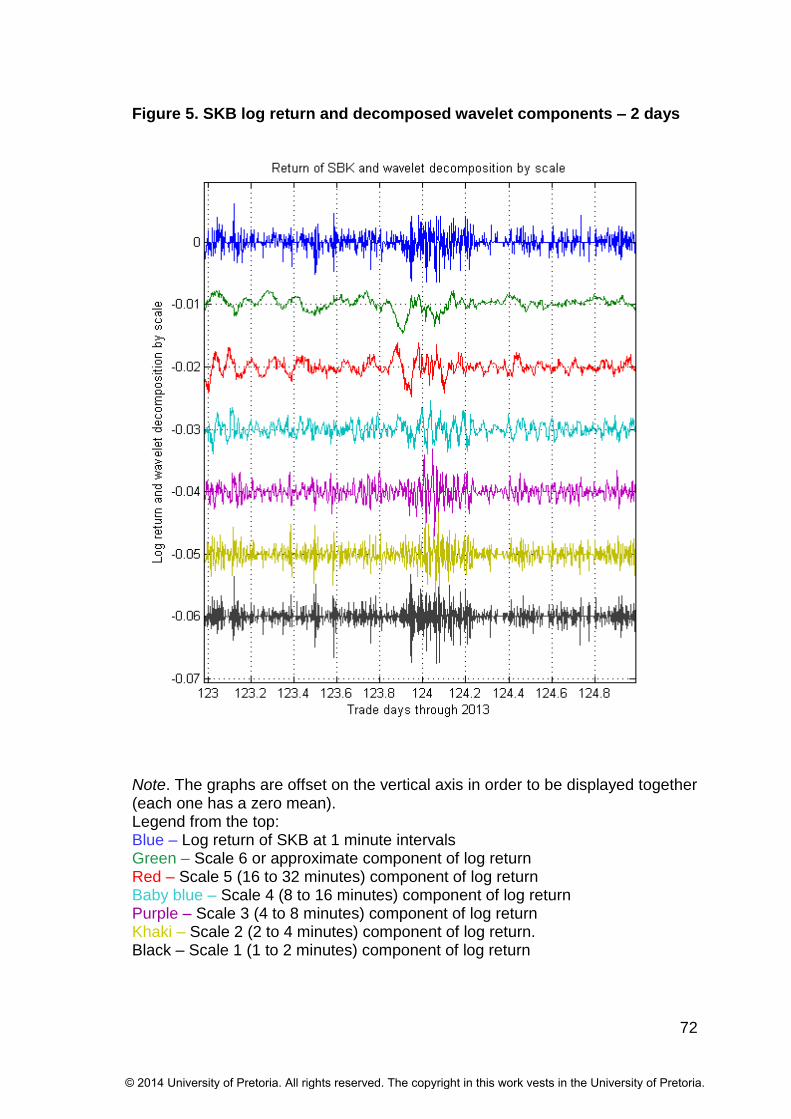
72
Figure 5. SKB log return and decomposed wavelet components – 2 days
Note. The graphs are offset on the vertical axis in order to be displayed together (each one has a zero mean). Legend from the top: Blue – Log return of SKB at 1 minute intervals Green – Scale 6 or approximate component of log return Red – Scale 5 (16 to 32 minutes) component of log return Baby blue – Scale 4 (8 to 16 minutes) component of log return Purple – Scale 3 (4 to 8 minutes) component of log return Khaki – Scale 2 (2 to 4 minutes) component of log return. Black – Scale 1 (1 to 2 minutes) component of log return
© 2014 University of Pretoria. All rights reserved. The copyright in this work vests in the University of Pretoria.
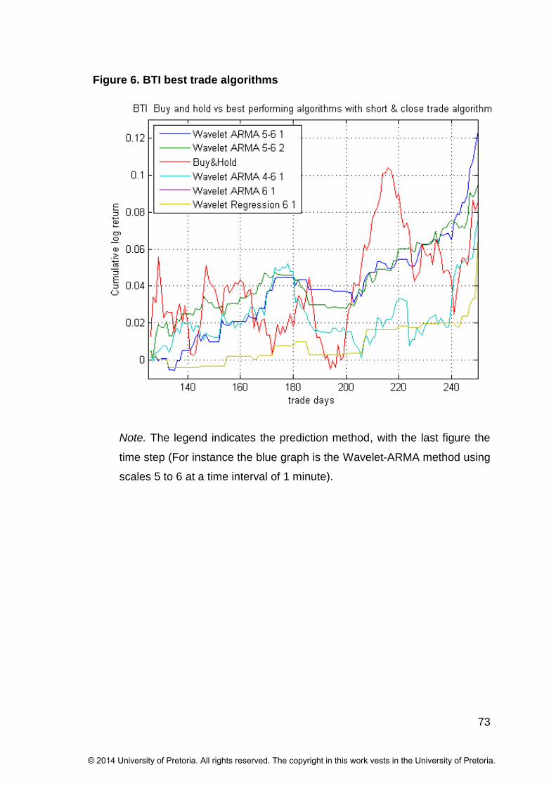
73
Figure 6. BTI best trade algorithms
Note. The legend indicates the prediction method, with the last figure the
time step (For instance the blue graph is the Wavelet-ARMA method using
scales 5 to 6 at a time interval of 1 minute).
© 2014 University of Pretoria. All rights reserved. The copyright in this work vests in the University of Pretoria.
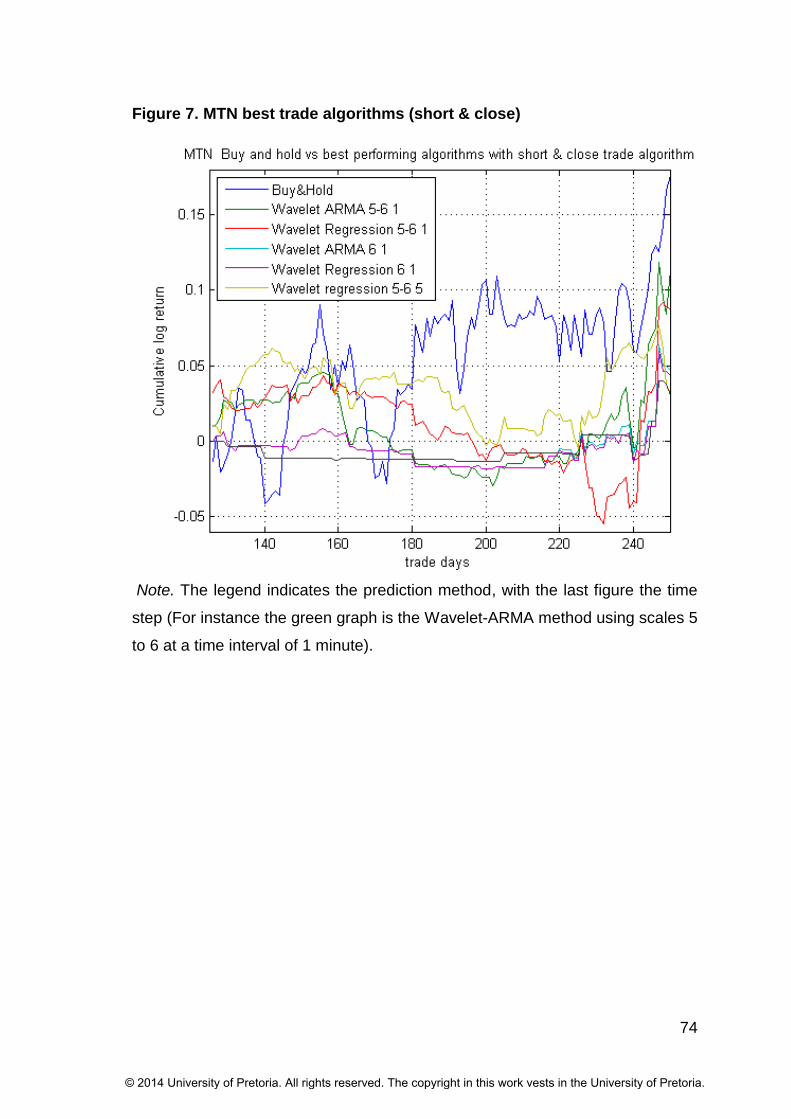
74
Figure 7. MTN best trade algorithms (short & close)
Note. The legend indicates the prediction method, with the last figure the time
step (For instance the green graph is the Wavelet-ARMA method using scales 5
to 6 at a time interval of 1 minute).
© 2014 University of Pretoria. All rights reserved. The copyright in this work vests in the University of Pretoria.
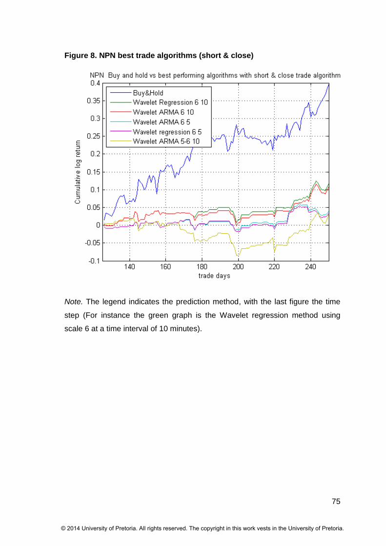
75
Figure 8. NPN best trade algorithms (short & close)
Note. The legend indicates the prediction method, with the last figure the time
step (For instance the green graph is the Wavelet regression method using
scale 6 at a time interval of 10 minutes).
© 2014 University of Pretoria. All rights reserved. The copyright in this work vests in the University of Pretoria.

76
Figure 9. SBK best trade algorithms (short & close)
Note. The legend indicates the prediction method, with the last figure the time
step (For instance the blue graph is the Wavelet-ARMA method using scales 5
to 6 at a time interval of 1 minute).
© 2014 University of Pretoria. All rights reserved. The copyright in this work vests in the University of Pretoria.

77
Figure 10. Number of trades through the test period
Note. The number of trades that the algorithms concluded through the 125 day
test period vs. the lowest scale of the wavelet-ARMA and wavelet regression
algorithms.
0 – ARMA
1 – scales 1 to 6
2 - scales 2 to 6
3 - scales 3 to 6
4 - scales 4 to 6
5 - scales 5 to 6
6 – scale 6.
The legend refers to the time step duration.
1
10
100
1000
10000
100000
0 1 2 3 4 5 6
nu
mb
er
of
trad
es
thro
ug
12
5 d
ays
Lowest scale
1 minute
2 minutes
5 minutes
10 minutes
© 2014 University of Pretoria. All rights reserved. The copyright in this work vests in the University of Pretoria.
Recommended