WEATHERING EFFECTS ON BIODEGRADATION AND TOXICITY OF HYDROCARBONS
IN GROUNDWATER
A Master’s Thesis Presented to the Faculty of California Polytechnic State University
San Luis Obispo
In partial fulfillment of the requirements for the degree of
Master of Science in Civil and Environmental Engineering
By
Marie Gabrielle Dreyer
June 2004
ii
COPYRIGHT OF MASTER’S THESIS
I hereby grant permission for the reproduction of this thesis in its entirety or any of its parts, without further authorization, provided acknowledgement is made to the author(s) and advisor(s). Marie G. Dreyer Date
iii
MASTER’S THESIS APPROVAL Title: Weathering Effects on Biodegradation and Toxicity of
Hydrocarbons in Groundwater
Author: Marie Gabrielle Dreyer
Date Submitted: June 2004
THESIS COMMITTEE MEMBERS:
Dr. Yarrow Nelson Date
Dr. Nirupam Pal Date
Dr. Chris Kitts Date
iv
ABSTRACT
WEATHERING EFFECTS ON BIODEGRADATION AND TOXICITY OF HYDROCARBONS IN GROUNDWATER
MARIE G. DREYER This study examined the effect of weathering on hydrocarbon biodegradation and toxicity at a former oil field near Guadalupe, California. Soil and groundwater at this site contains residual diesel-range hydrocarbons from refinery products used to dilute the viscous crude oil at this site to facilitate pumping. Natural attenuation is being considered at this site as a means of remediating residual hydrocarbons (diluent) in soil and groundwater following more active remediation techniques. To provide the lines of evidence required for use of natural attenuation at this site, this research was undertaken to determine if the hydrocarbons continue to be biodegradable after extensive weathering in the field. To investigate changes in diluent characteristics with aging, a total of thirty four groundwater samples were collected from across the site with a range of total petroleum hydrocarbon (TPH) concentrations. It was assumed that samples with low TPH concentrations were more weathered than samples with high TPH concentrations. The biodegradability of TPH in each sample was determined by measuring respiration rates (through CO2 production) and twenty day TPH degradation rates measured in the laboratory. Changes in TPH composition with weathering were evaluated using gas chromatography (GC) with simulated distillation (SIMDIS) to determine equivalent carbon chain length. Total organic carbon (TOC) analysis was used to determine concentrations of other organic material in the groundwater samples. Finally, Microtox® toxicity was measured to determine the effect of weathering of the hydrocarbon mixtures on toxicity. Respirometry experiments for groundwater samples from twenty wells indicated the presence of microbial activity as measured over time intervals of six or twenty days. An initial phase of constant microbial activity was seen within the first 36 hours of measurements, followed by a second phase of declined activity by most samples. This decline in degradation, when samples presumably contain lower (than initially measured) TPH concentrations, would be expected for first order kinetics where rate increases with increasing concentration. In fact, twenty day biodegradation rates were directly proportional to initial TPH concentrations (R2 = 0.9197) indicative of first-order kinetics. The first-order rate constant was 0.023 day-1 based on all groundwater samples analyzed. Two samples with low initial TPH concentrations exhibited first-order rate constants significantly lower than expected from the first order rate constant, which is possibly due to low nutrient concentrations. TPH degradation rates and CO2 respiration rates decreased with increasing downgradient distance from contaminant source. This is expected because TPH concentrations also
v
decreased with increasing distance from the source, so lower rates would be expected based on first order kinetics. However, by plotting first order rate constant versus distance from source zone for four plumes it was seen that first-order rate constants decreased from 5 to 46 % along plume transects. This suggests the first order rate constants decrease significantly with weathering. This indicates a reduction of hydrocarbon biodegradability in groundwater down gradient from the source, however biodegradation rates are capable of degradation at a reduced rate. Microtox® toxicity decreased significantly with decreasing TPH concentrations. However, some samples with similar TPH concentration exhibited widely different toxicity suggesting hydrocarbon composition affects toxicity. All samples with initially high toxicity exhibited dramatic decreases in toxicity during twenty days of biodegradation in the laboratory. Samples with low initial toxicity exhibited a slight decrease or, in some instances, an increase in toxicity. These findings indicate a difficulty in biodegrading samples below a certain threshold of toxicity. However, the initial toxicity concentrations for these samples were low enough that many were considered (by the analyzer) as nontoxic. After the period of most active biodegradation (twenty days) slight amounts of both TPH and toxicity remained. These results may be helpful for determining appropriate remediation endpoints. The rapid decreases in toxicity and TPH concentrations for samples with initially high values indicates the use of natural attenuation may still be feasible regardless of residual TPH or toxicity concentrations.

vi
ACKNOWLEDGEMENTS
I want to give a special thanks to the following special individuals:
Dr. Yarrow Nelson for his constant guidance and
patiently sitting though my senioritis.
Dr. Nirupam Pal and Dr. Chris Kitts for their support.
Bob Pease (BFJ Services), for his continued support in all these efforts
at the Guadalupe site.
My fellow graduate students, good luck to you all.
Mom, Dad and Kenny for their constant “I think I can” attitudes.
Al, Meryll, Jimmy, Bunkim and Dave
for their “insightful” comments and keeping things fun.
Eric, for being you.
And to Paul Lundegard, Gonzalo Garcia and the Unocal team, for the opportunity to
work on this amazing site and for funding this phenomenal study.
vii
TABLE OF CONTENTS LIST OF TABLES.............................................................................................................. x
LIST OF FIGURES ........................................................................................................... xi
INTRODUCTION .............................................................................................................. 1
PROJECT SCOPE .............................................................................................................. 3
BACKGROUND ................................................................................................................ 5
3.1 Principles behind Monitored Natural Attenuation (MNA)....................................... 6
3.1.1 Current Regulations for MNA ........................................................................... 8
3.1.1.1 Lines of Evidence ....................................................................................... 9
3.1.1.2 Remediation Objectives .............................................................................. 9
3.1.1.3 Monitoring ................................................................................................ 10
3.1.1.4 Unsuccessful Remediation........................................................................ 10
3.1.2 Advantages of MNA........................................................................................ 10
3.1.3 Limitations of MNA ........................................................................................ 11
3.2 Guadalupe Restoration Project (GRP) Site, Guadalupe, California ....................... 11
3.2.1 Characterization of Dissolved Phase Diluent Contamination.......................... 13
3.3 Biodegradation Analyses ........................................................................................ 14
3.3.1 Previous Work on TPH Biodegradation at GRP ............................................. 14
3.3.2 CO2 Production as a Measurement of Biodegradation .................................... 15
3.3.3 Total Organic Carbon ...................................................................................... 16
3.3.4 Toxicity as a Measurement of Biodegradation ................................................ 16
3.3.5 2D Gas Chromatography Analysis at Woods Hole Oceanographic Institute .. 17
viii
MATERIALS AND METHODS...................................................................................... 18
4.1 Groundwater Samples............................................................................................. 18
4.2 Respirometry Experiments...................................................................................... 22
4.2.1 Respirometry Methods..................................................................................... 22
4.2.2 Respirometry Sample Preparation for Subset 1 ............................................... 23
4.2.3 Respirometry Sample Preparation for Subset 3 ............................................... 25
4.3 Total Organic Carbon (TOC) Measurement ........................................................... 25
4.3.1 TOC Methods................................................................................................... 25
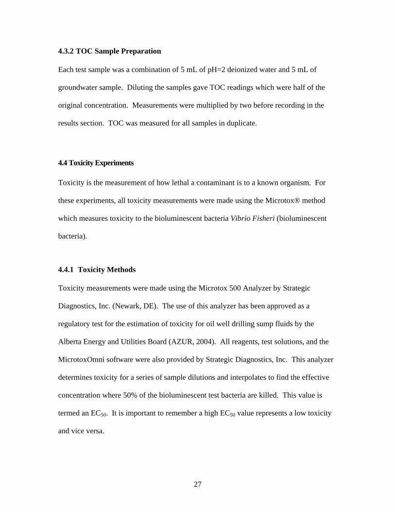
4.3.2 TOC Sample Preparation ................................................................................. 27
4.4 Toxicity Experiments.............................................................................................. 27
4.4.1 Toxicity Methods ............................................................................................. 27
4.4.2 Microtox® Sample Preparation ....................................................................... 28
4.5 Total Petroleum Hydrocarbon (TPH) Analysis ...................................................... 29
4.6 Twenty Day Biodegradation Rate Analysis............................................................ 29
RESULTS AND DISCUSSION....................................................................................... 31
5.1 Respirometry Results .............................................................................................. 33
5.1.1 Respirometry Results for Subset 1A................................................................ 33
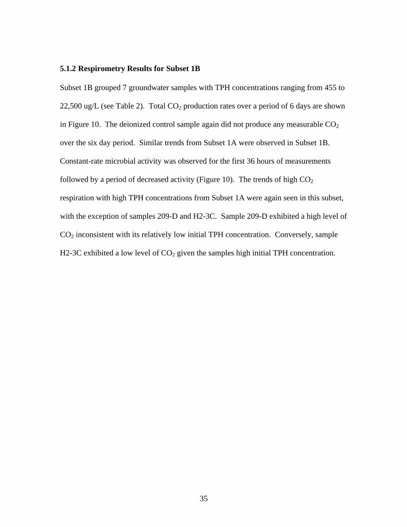
5.1.2 Respirometry Results for Subset 1B................................................................ 35
5.1.3 Respirometry Results for Subset 3................................................................... 37
5.1.4 CO2 Respiration Rate vs. Initial TPH Concentration....................................... 39
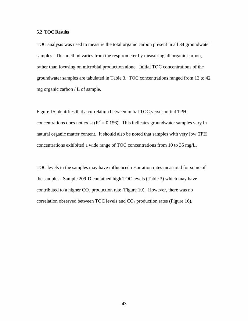
5.2 TOC Results............................................................................................................ 43
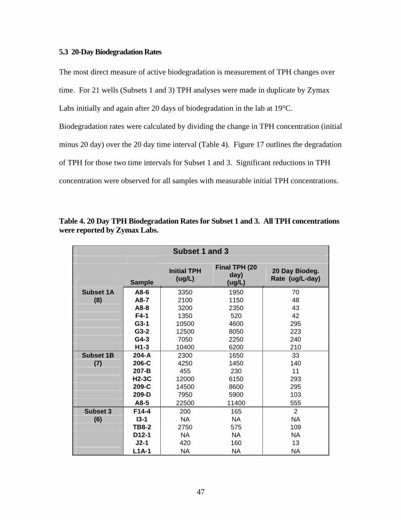
5.3 20-Day Biodegradation Rates ................................................................................. 47
5.3.1 Simulated Distillation (SIMDIS) Analysis ...................................................... 55
ix
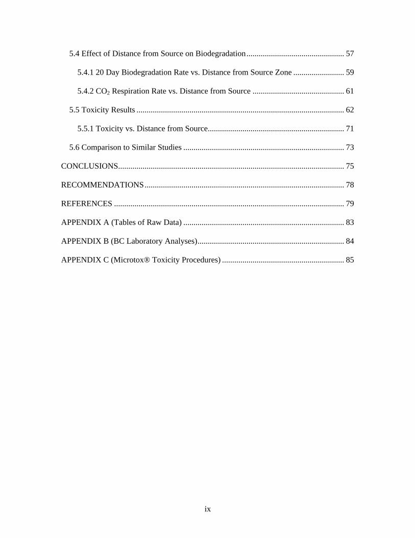
5.4 Effect of Distance from Source on Biodegradation................................................ 57
5.4.1 20 Day Biodegradation Rate vs. Distance from Source Zone ......................... 59
5.4.2 CO2 Respiration Rate vs. Distance from Source ............................................. 61
5.5 Toxicity Results ...................................................................................................... 62
5.5.1 Toxicity vs. Distance from Source................................................................... 71
5.6 Comparison to Similar Studies ............................................................................... 73
CONCLUSIONS............................................................................................................... 75
RECOMMENDATIONS.................................................................................................. 78
REFERENCES ................................................................................................................. 79
APPENDIX A (Tables of Raw Data) ............................................................................... 83
APPENDIX B (BC Laboratory Analyses)........................................................................ 84
APPENDIX C (Microtox® Toxicity Procedures) ............................................................ 85
x
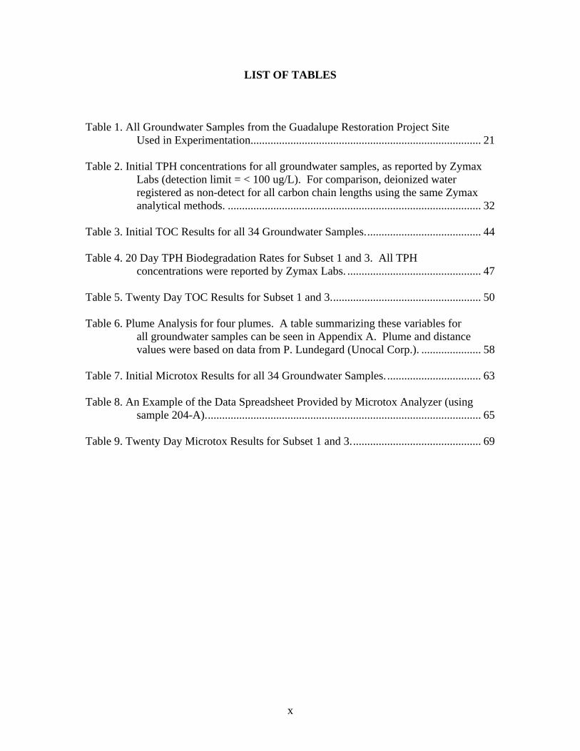
LIST OF TABLES
Table 1. All Groundwater Samples from the Guadalupe Restoration Project Site Used in Experimentation................................................................................. 21
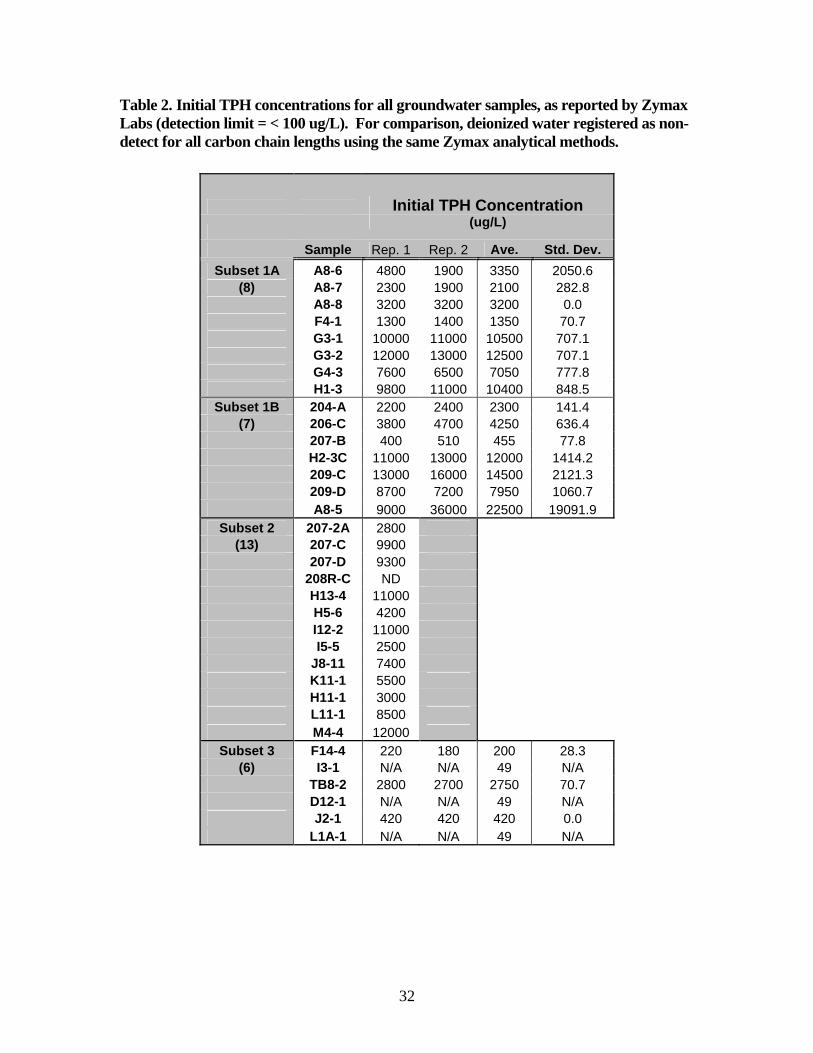
Table 2. Initial TPH concentrations for all groundwater samples, as reported by Zymax
Labs (detection limit = < 100 ug/L). For comparison, deionized water registered as non-detect for all carbon chain lengths using the same Zymax analytical methods. ......................................................................................... 32
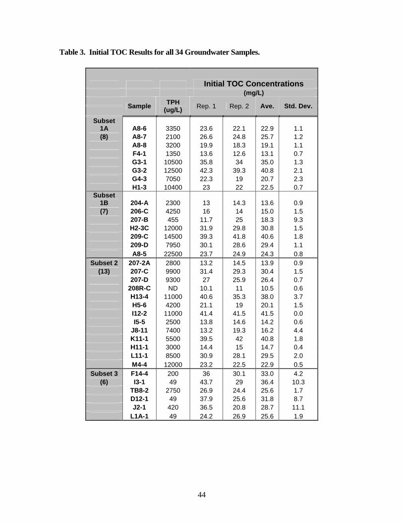
Table 3. Initial TOC Results for all 34 Groundwater Samples......................................... 44 Table 4. 20 Day TPH Biodegradation Rates for Subset 1 and 3. All TPH
concentrations were reported by Zymax Labs. ............................................... 47 Table 5. Twenty Day TOC Results for Subset 1 and 3..................................................... 50 Table 6. Plume Analysis for four plumes. A table summarizing these variables for
all groundwater samples can be seen in Appendix A. Plume and distance values were based on data from P. Lundegard (Unocal Corp.). ..................... 58
Table 7. Initial Microtox Results for all 34 Groundwater Samples. ................................. 63 Table 8. An Example of the Data Spreadsheet Provided by Microtox Analyzer (using
sample 204-A)................................................................................................. 65 Table 9. Twenty Day Microtox Results for Subset 1 and 3.............................................. 69
xi
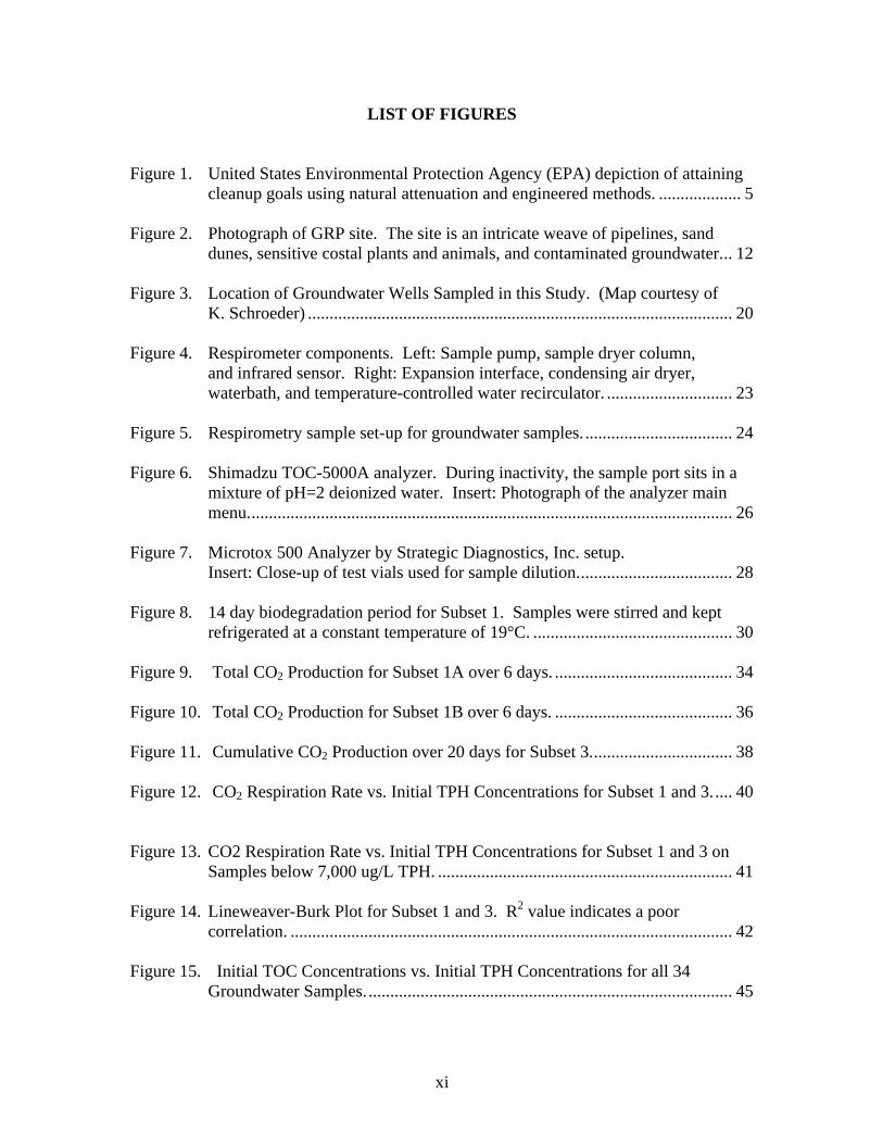
LIST OF FIGURES Figure 1. United States Environmental Protection Agency (EPA) depiction of attaining
cleanup goals using natural attenuation and engineered methods. ................... 5 Figure 2. Photograph of GRP site. The site is an intricate weave of pipelines, sand
dunes, sensitive costal plants and animals, and contaminated groundwater... 12 Figure 3. Location of Groundwater Wells Sampled in this Study. (Map courtesy of
K. Schroeder) .................................................................................................. 20 Figure 4. Respirometer components. Left: Sample pump, sample dryer column,
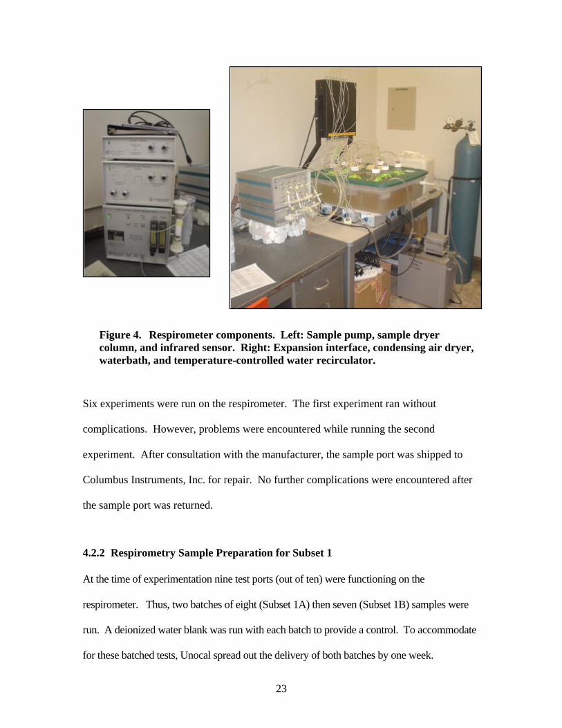
and infrared sensor. Right: Expansion interface, condensing air dryer, waterbath, and temperature-controlled water recirculator. ............................. 23
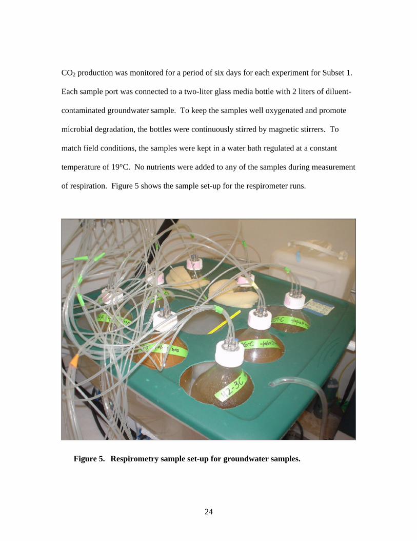
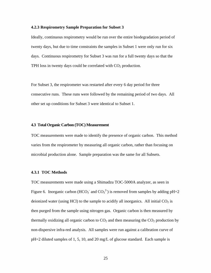
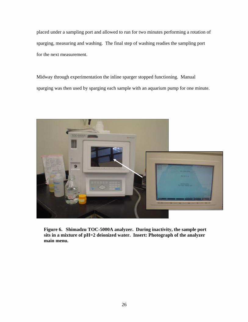
Figure 5. Respirometry sample set-up for groundwater samples. .................................. 24 Figure 6. Shimadzu TOC-5000A analyzer. During inactivity, the sample port sits in a
mixture of pH=2 deionized water. Insert: Photograph of the analyzer main menu................................................................................................................ 26
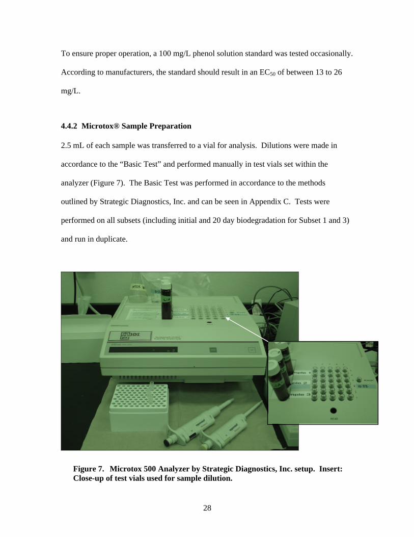
Figure 7. Microtox 500 Analyzer by Strategic Diagnostics, Inc. setup.
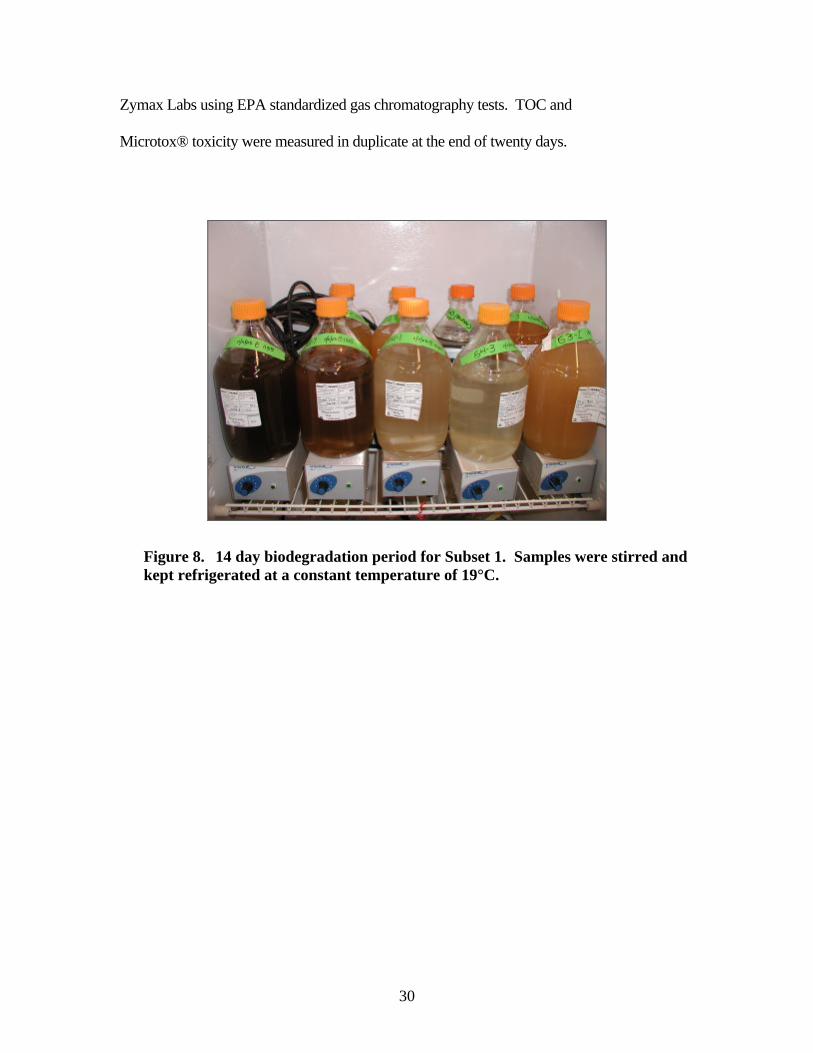
Insert: Close-up of test vials used for sample dilution.................................... 28 Figure 8. 14 day biodegradation period for Subset 1. Samples were stirred and kept
refrigerated at a constant temperature of 19°C. .............................................. 30 Figure 9. Total CO2 Production for Subset 1A over 6 days. ......................................... 34 Figure 10. Total CO2 Production for Subset 1B over 6 days. ......................................... 36 Figure 11. Cumulative CO2 Production over 20 days for Subset 3................................. 38 Figure 12. CO2 Respiration Rate vs. Initial TPH Concentrations for Subset 1 and 3. .... 40 Figure 13. CO2 Respiration Rate vs. Initial TPH Concentrations for Subset 1 and 3 on
Samples below 7,000 ug/L TPH. .................................................................... 41 Figure 14. Lineweaver-Burk Plot for Subset 1 and 3. R2 value indicates a poor
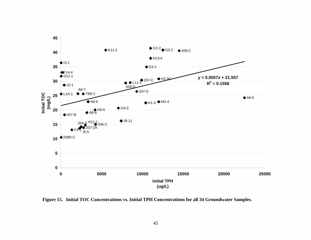
correlation. ...................................................................................................... 42 Figure 15. Initial TOC Concentrations vs. Initial TPH Concentrations for all 34
Groundwater Samples. .................................................................................... 45

xii
Figure 16. CO2 Respiration Rate vs. Initial TOC Concentration for all 34 Groundwater Wells. .............................................................................................................. 46
Figure 17. TPH Concentrations for Subset 1 and 3. Measurements were taken initially
and at 20 days of biodegradation. All analyses were performed by Zymax Labs................................................................................................................. 51
Figure 18. 20 Day TPH Biodegradation vs. Initial TPH Concentrations for Subset 1
and 3. Trendline and R-squared = 0.9197 indicates a direct proportionality in data.............................................................................................................. 52
Figure 19. 20 Day TPH Biodegradation vs. Initial TPH Concentrations for Low TPH
Concentration samples. ................................................................................... 53 Figure 20. Correlation between CO2 Respiration Rate and 20 Day Biodegradation
Rate. Used to identify the validity of respirometry as indicator for TPH biodegradation................................................................................................. 54
Figure 21. Carbon Chain Distribution for Sample G3-2 (Initial TPH = 12,500 ug/L). ... 56 Figure 22. Carbon Chain Distribution for Sample F4-1 (Initial TPH = 1,350 ug/L). ...... 56 Figure 23. Location of Four Plumes Analyzed. Plumes analyzed are circled in red. ..... 57 Figure 24. 20 Day Biodegradation Rate vs. Distance from Source Zone for Selected
Plumes............................................................................................................. 60 Figure 25. Specific TPH Utilization Rate vs. Distance from Source Zone for Selected
Plumes. Rate was calculated by dividing degradation rate by TPH concentration................................................................................................... 60
Figure 26. CO2 Respiration Rate vs. Distance from Source. ........................................... 61 Figure 27. Initial Microtox EC50 vs. Initial TPH Concentration for all 34 Groundwater
Samples ........................................................................................................... 64 Figure 28. A Sample Plot for % Effect vs. Concentration (using sample 204-A). .......... 66 Figure 29. Toxicity as measured by Initial % Effect at Full Concentration vs. Initial
TPH Concentration for all groundwater samples............................................ 68 Figure 30. % Effect at Full Concentration for Subset 1 and 3. Measurements were
taken initially and at 20 days of biodegradation. ............................................ 70 Figure 31. Toxicity (Initial % Effect) vs. Distance from Source. .................................... 71
1
CHAPTER 1
INTRODUCTION
Natural attenuation is a method of remediation reliant on natural biological, chemical and
physical processes to biodegrade or otherwise reduces concentrations of contaminants at
hazardous waste sites. It is a remediation method rapidly increasing in popularity
because of its capability to remediate a contaminated site with little to no disturbance.
Use of natural attenuation is currently being investigated at the Guadalupe Restoration
Project (GRP) site. Hydrocarbon mixtures similar to diesel fuel were used at this former
oil field as a diluent for facilitating pumping of the viscous crude oil extracted at
Guadalupe. Unfortunately, large quantities of this diluent were accidentally released and
led to extensive soil and groundwater contamination at the site. The diluent is a
moderately viscous compound containing volatile organic compounds (VOCs) and
polycyclic aromatic hydrocarbons (PAHs). From the 1950s to about 1990 diluent was
used to ease the transport of viscous heavy crude oil in pipelines throughout the site.
Leaks occurred at various times and volumes. However, some were sufficient enough in
quantity to percolate through the sand dunes into the groundwater table. Plumes sizes
vary from 1 to 100,000 m3 (hundreds of gallons to a few million gallons) of diluent. The
GRP site is home to a number of endangered or sensitive species and flora. As a highly
sensitive site requiring restoration, natural attenuation seems like a good remediation
method for the GRP site.
For natural attenuation to be successful, biodegradation must be sustained, even at low
contaminant concentrations (weathered material). To help determine the feasibility of
2
natural attenuation at GRP, an evaluation of physical and chemical factors affecting
sustainability of natural attenuation of dissolved phase diluent is being made by
examining biodegradation and toxicity. Together with Unocal, the Environmental
Biotechnology Institute (EBI) and Dr. Yarrow Nelson, this project is expected to further
the research into sustainable natural attenuation at the GRP site.
3
CHAPTER 2
PROJECT SCOPE
Fundamental to the question of ongoing natural attenuation at the Guadalupe site is
sustainability. Previous tests at the site have shown initial rapid biodegradation
(following first-order kinetics), followed by an asymptotic curve of reduced activity
(simulating a zero-order kinetic reaction) (Cunningham, 2004; Waudby, 2003). Given
the consistency of this trend, it is important to explore possible reasons behind the
pattern. Therefore, a key area of research is to examine the trends of biodegradation and
toxicity for GRP groundwater samples initially and after weathering in the field. Critical
questions to be answered include: What causes the observed initial first-order kinetic
hydrocarbon biodegradation to diminish after 20 days? Are nutrients limiting
biodegradation? Are easily degraded components of the diluent preferentially
biodegraded leaving a more recalcitrant compound? Is toxicity reduced through
biodegradation?
This research addresses the effects of weathering on biodegradability and toxicity using a
combination of field and laboratory tests. Samples of groundwater at varying stages of
biodegradation were collected from a series of thirty four monitoring wells. Groundwater
samples collected at varying distances from the source are expected to have varying
degrees of weathering and stages of degradation. The field samples were analyzed for
total petroleum hydrocarbon (TPH) (including simulated distillation (SIMDIS)
integration), respiration rate, TPH degradation rate (over twenty days) and Microtox®
toxicity to infer changes in diluent characteristics with aging during natural attenuation.
4
Water chemistry of these samples was also fully characterized to test for nutrient
concentrations. Microbial characterization is being evaluated in a companion study by
the Department of Microbiology at California Polytechnic State University, San Luis
Obispo (Cal Poly, SLO).
This project is part of a larger natural attenuation study of weathering effects on
biodegradation currently being conducted by Yarrow Nelson and Chris Kitts. A
companion laboratory study simulated field conditions using laboratory soil columns to
examine temporal changes in one sample of hydrocarbon-rich groundwater
(Cunningham, 2004). Another companion study is using an advanced two-dimensional
gas chromatography method to provide detailed chemical analyses of the weathered
hydrocarbons.
5
CHAPTER 3
BACKGROUND
Natural attenuation is a powerful remediation alternative for many sites with
contaminated soil and groundwater. Often, in the face of engineered processes, natural
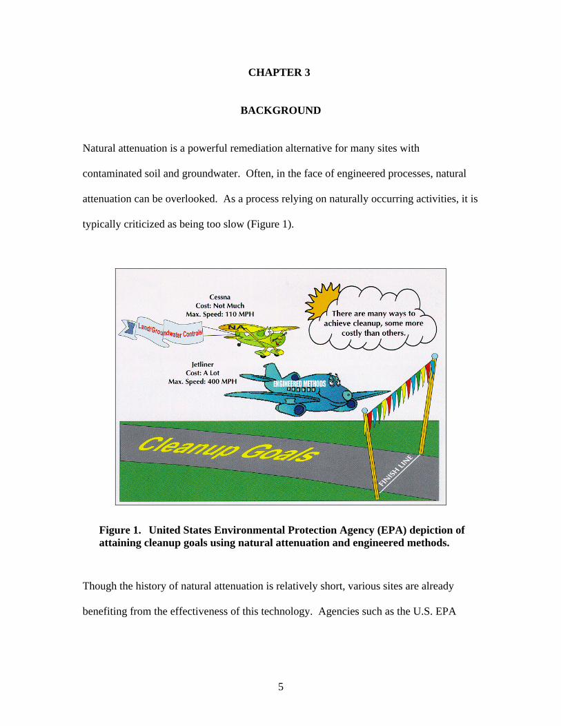
attenuation can be overlooked. As a process relying on naturally occurring activities, it is
typically criticized as being too slow (Figure 1).
Figure 1. United States Environmental Protection Agency (EPA) depiction of attaining cleanup goals using natural attenuation and engineered methods.
Though the history of natural attenuation is relatively short, various sites are already
benefiting from the effectiveness of this technology. Agencies such as the U.S. EPA
6
have teamed together to create standard methods for treating contaminated sites through
natural attenuation processes (AFCEE, 2002).
3.1 Principles behind Monitored Natural Attenuation (MNA)
Natural attenuation has recently become a popular method of remediation. By 1995,
using natural attenuation to treat contaminated soils became a favored option at U.S.
Superfund sites. Approximately 29,000 (or 28 %) of all sites currently use natural
attenuation. It proves even more valuable for contaminated groundwater sites, being the
most favored above all other technologies. Approximately 17,000 sites, or about 47 % of
all contaminated groundwater sites, use this technology for treatment in the U.S.
(USEPA, October 2003; Tulis, 2002).
Natural attenuation works by using natural biological, chemical, and physical processes
to remediate and treat contaminants in soils and groundwater. It is considered a
“passive” or “non-invasive” remediation method, meaning it works without significant
intervention or associated harm to the environment. The successful remediation of many
sites has proven this technology capable of diminishing inorganic and organic
contaminants, the most notable being petroleum-based compounds (AFCEE, 2002).
Because of its name and non-invasive approach, people often mistake natural attenuation
as the “No Further Action” (NFA) approach. A NFA site is one deemed “protective of
human health and the environment.” On the contrary, a natural attenuation site is by
definition “not protective” of those resources. It must still be actively characterized,
assessed for risks, and monitored, but without relying solely on “engineered” remediation
7
processes. Confusion between these two processes has led to the renaming of natural
attenuation to “monitored natural attenuation” (MNA) (USEPA, October 2003; CPEO,
2003; Tulis, 2002).
MNA is a culmination of various treatment processes. These processes (in one way or
another) fit the description of providing ample treatment of contaminated soils and
groundwater while still remaining relatively non-invasive. Some of these processes are
listed below (AFCEE, 2002).
• Dilution and Dispersion - the lowering of contaminant concentrations as the
contaminants migrate away from the source.
• Absorption or Adsorption - the reduction of environmental contaminants due to
contaminant incorporation and adhesion to soil particles.
• Volatilization - the reduction of environmental contaminants through
vaporization or evaporation into the atmosphere.
• Chemical Transformation - the decomposition of contaminants through a series
of naturally occurring chemical reactions.
• Biodegradation or Bioremediation - the decomposition of environmental
contaminants by soil microorganisms.
Extensive studies into the successful use of natural attenuation have been done by the
United States Geological Survey (USGS) agency. At many sites, USGS was able to
quantitatively demonstrate the ability of microorganisms to actively consume toxic
compounds and convert them into CO2. In one year a USGS site in South Carolina,
8
suffering from leaky military fuel storage facilities, was able to reduce contaminant
concentrations seventy-five percent. Another study at a site in Bemidji, Minnesota
confirmed that crude oil was rapidly degraded by indigenous microbial populations.
Further success of natural attenuation at the site was also witnessed when contaminated
groundwater was hindered from further spreading as biodegradation rates came into
equilibrium with rates of contaminant leaching. A chlorinated solvents contaminated site
in New Jersey showed the adaptability of microorganisms. At this site, microbes utilized
readily available chlorinated compounds as oxidants when other oxidants were not
present. Another site in New Jersey contaminated with gasoline showed the importance
of microbial populations in the unsaturated zone toward biodegradation. Together these
sites laid the technical foundation for USGS scientists to continue their consideration for
the use of natural attenuation at contaminated sites (USGS, 1997).
3.1.1 Current Regulations for MNA
Site contamination has become more problematic as responsible parties watch their
remediation costs increase. Though every site is specific to its area and history, soil and
groundwater contamination is a national problem. As such, the EPA, Air Force, Army,
Navy and Coast Guard as well as industrial players have all put forward their ideas of a
successful MNA program. Though each program has distinctive differences, they are
bound by the following requirements: providing lines of evidence, listing remediation
objectives, a continual monitoring program, and a backup plan if remediation by natural
attenuation proves unsuccessful (AFCEE, 2002).
9
3.1.1.1 Lines of Evidence
Sites deemed favorable for the use of natural attenuation must first meet at least one of
the following “lines of evidence” (AFCEE, 2002).
1. “Historical groundwater and/or soil chemistry data may be used to demonstrate a
clear and meaningful trend of decreasing contaminant mass and/or concentration
has been observed over time at appropriate monitoring or sampling ports.”
2. “Hydrogeologic and geochemical modeling data can be used to demonstrate
indirectly the type(s) of natural attenuation processes active at the site and the rate
these processes will reduce contaminant concentrations to required levels.”
3. “Data from field or microcosm studies (conducted in or with actual contaminated
site media) may be used to demonstrate the occurrence of a particular natural
attenuation process at the site and its ability to degrade the contaminants of
concern.”
3.1.1.2 Remediation Objectives
Once the site is deemed appropriate for MNA, a plan must be created with clearly defined
objectives. Objectives include identifying remediation levels or performance
requirements, determining points of compliance, and establishing an acceptable
timeframe for remediation (Tulis, 2002). Additionally, the MNA plan must comply with
any state groundwater or soil use classification and remediation standards (USEPA,
March 2003).
10
3.1.1.3 Monitoring
Given the generally slow progression of MNA, long-term monitoring is essential. This
type of monitoring ensures the processes are performing up to par and are meeting
expected remediation goals. To facilitate the process, frequent (usually quarterly)
sampling takes place to determine current site conditions, plume migrations, byproduct
creation, and any increased risks to human health or the environment. Analysis generally
includes geochemical, hydro-geological, and microbiological changes of the site and
contaminants. Ultimately, monitoring reveals whether MNA is working or if a more
“active” means of remediation must be investigated (AFCEE, 2002).
3.1.1.4 Unsuccessful Remediation
Should MNA fail, it can become necessary to throw in the towel. More than likely,
should MNA fail, an applicable engineered process will be employed to complete the job
(USEPA, March 2003).
3.1.2 Advantages of MNA
MNA has several key advantages over engineered processes. The use of naturally
occurring microorganisms and soil/groundwater interactions generates less remediation
waste, reduces human exposure to contaminants, and limits environmental disturbance.
Little to no equipment is needed to successfully operate a MNA site, resulting in less
equipment failure and downtime. By limiting reliance on equipment, MNA significantly
reduces remediation costs, particularly when compared to more active remediation
technologies. As a simple, yet effective, technology MNA can be the sole restoration
11
alternative or utilized in conjunction with more active technologies (USEPA, March
2003; AFCEE, 2002; Tulis, 2002).
3.1.3 Limitations of MNA
Although MNA has an extensive list of advantages, it also has limitations. Of primary
concern is time of completion. Typically, MNA requires a longer time frame to achieve
established remediation goals (Figure 1). Site evaluation and providing lines of evidence
are often complex and costly with MNA. Often, site characteristics change over time and
may require the implementation of a more active remediation method. Required long-
term monitoring of MNA can also extend the time of completion. Prolonged times of
planning, evaluation and other publicly-viewed inactivity may cause misinterpretation
from the public. This uncertainty delays future land uses and property transfers, and can
create liability issues (USEPA, March 2003; AFCEE, 2002; Tulis, 2002).
3.2 Guadalupe Restoration Project (GRP) Site, Guadalupe, California
About 30 miles south of San Luis Obispo lies a site greatly contaminated by petroleum
hydrocarbons used as diluent. The GRP site is a former oil field which was active from
1950 to about 1990. The composition of the crude oil at the site is such that an oil thinner
(diluent) was needed to facilitate pumping. During that time, diluent leaked and
percolated through the dune sand and along the groundwater table. Plumes are located
throughout the site and range in size from hundreds to a few million gallons. During the
period of production no remedial efforts were made, and diluent continued to flow into
the soil and groundwater at the site. Now, almost 50 years later, agencies are finally
12
holding Unocal responsible for their actions. As part of the lawsuit issued on them, they
must restore the site to safe conditions both for humans and the natural ecosystem (Catts
et al., 2003).
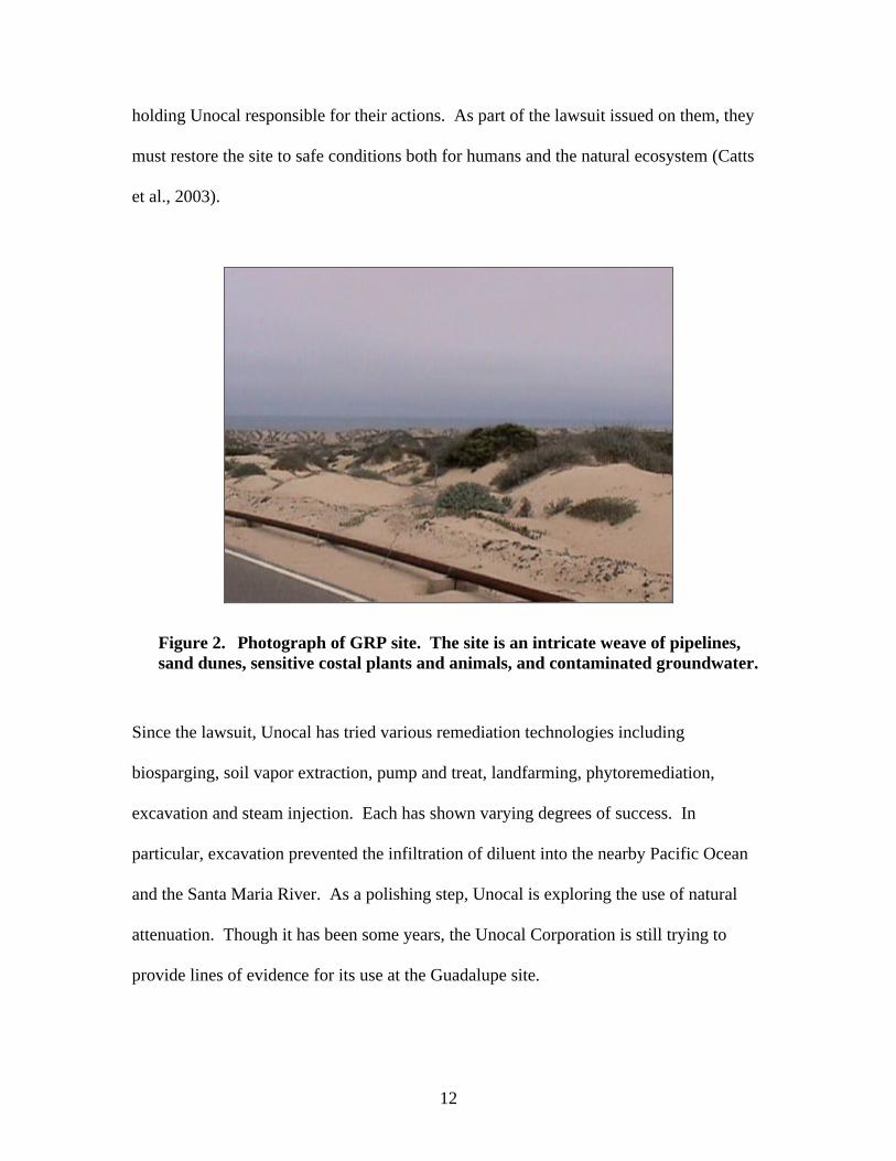
Figure 2. Photograph of GRP site. The site is an intricate weave of pipelines, sand dunes, sensitive costal plants and animals, and contaminated groundwater.
Since the lawsuit, Unocal has tried various remediation technologies including
biosparging, soil vapor extraction, pump and treat, landfarming, phytoremediation,
excavation and steam injection. Each has shown varying degrees of success. In
particular, excavation prevented the infiltration of diluent into the nearby Pacific Ocean
and the Santa Maria River. As a polishing step, Unocal is exploring the use of natural
attenuation. Though it has been some years, the Unocal Corporation is still trying to
provide lines of evidence for its use at the Guadalupe site.
13
3.2.1 Characterization of Dissolved Phase Diluent Contamination
The diluent used at Guadalupe was a complex mixture of hydrocarbons with equivalent
chain lengths from C10 to C30. The majority (90 %) of the hydrocarbons are within
equivalent chain lengths of C14 to C30. These ranges are consistent with diesel and
kerosene hydrocarbons. It has a specific gravity of 0.9 at 60°F and ranges in TPH
concentrations from 910,000 to 990,000 mg/kg. Problems with biodegradation are
encountered in part due to the forty one identifiable polycyclic aromatic hydrocarbons
(PAH) (Lundegard and Garcia, 2001). Testing by Zymax Envirotechnology, San Luis
Obispo, California (Zymax Labs) identified naphthalene as being the PAH in greatest
abundance (accounting for 90 % of the sum total of PAHs).
The presence of PAH residues in petroleum spill sites are problematic to soil remediation.
Their persistence is largely due to the difficulty of breaking ring structures (Wang and
Bartha, 1990). The presence of PAHs can increase the toxicity of a hydrocarbon mixture
(Kropp and Fedorak, 1998). However, given the right conditions for microbial
degradation, pH control, nutrient balance, aeration and mixing, bioremediation can be a
very cost-effective remediation procedure for PAHs (Dragun, 1998).
The variety of PAHs and the variance in chain lengths in petroleum products have caused
researchers to question the feasibility of biodegradation at oil spill sites. Typically, short
chain hydrocarbons (C10 to C18) are more bioavailable, which directly correlates to their
ease of biodegradation (Nocentini et al., 2000; Siddiqui and Adams, 2001; Wang and
Bartha, 1990). This finding is significant considering equivalent carbon chain lengths at
14
the GRP site reached C30. Most sites experience rapid first-order biodegradation near
the source zone (Lundegard and Johnson, 2003; Yerushalmi et al., 2003). However, at
farther distances biodegradation slows considerably (Lundegard and Johnson, 2003). At
farther distances, petroleum deposits are considered “weathered” by both microorganisms
and physical processes. Other groundwater contaminated sites witnessed a residual
fraction of contaminants which remained undegraded at these weathering locations
(Huesemann, 1997; Nocentini et al., 2000).
3.3 Biodegradation Analyses
Many methods are available for measuring hydrocarbon biodegradation rates in the
laboratory including direct TPH measurements, respirometry, TOC and toxicity. Each of
these methods is described in the following subsections.
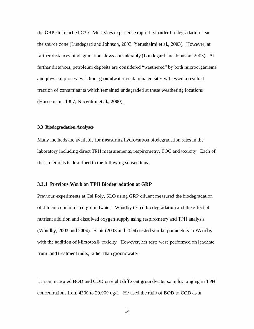
3.3.1 Previous Work on TPH Biodegradation at GRP
Previous experiments at Cal Poly, SLO using GRP diluent measured the biodegradation
of diluent contaminated groundwater. Waudby tested biodegradation and the effect of
nutrient addition and dissolved oxygen supply using respirometry and TPH analysis
(Waudby, 2003 and 2004). Scott (2003 and 2004) tested similar parameters to Waudby
with the addition of Microtox® toxicity. However, her tests were performed on leachate
from land treatment units, rather than groundwater.
Larson measured BOD and COD on eight different groundwater samples ranging in TPH
concentrations from 4200 to 29,000 ug/L. He used the ratio of BOD to COD as an
15
indication of biodegradability. Larson found that there was no decrease in BOD/COD
ratio with decreasing TPH concentration. However, he did report a slight reduction in
biodegradability with distance from source zone. But, BOD and COD are very indirect
measures of biodegradability and TPH concentration (Larson, 2003).
All of these experiments helped lay the groundwork for this study. By applying Scott and
Waudby’s respirometry methods and Scott’s Microtox® toxicity analysis to Larson’s
methodology of testing a wide array of samples, this study is better able to assess the
affects of biodegradation on TPH contaminated groundwater.
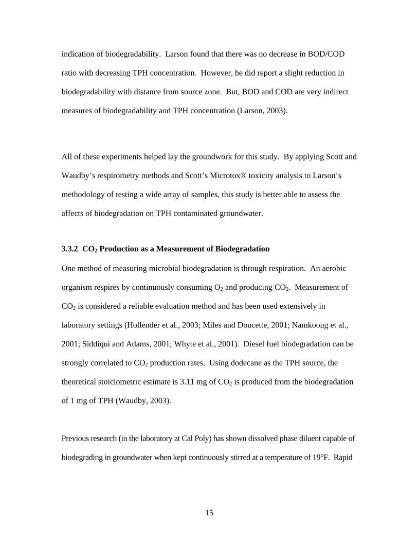
3.3.2 CO2 Production as a Measurement of Biodegradation
One method of measuring microbial biodegradation is through respiration. An aerobic
organism respires by continuously consuming O2 and producing CO2. Measurement of
CO2 is considered a reliable evaluation method and has been used extensively in
laboratory settings (Hollender et al., 2003; Miles and Doucette, 2001; Namkoong et al.,
2001; Siddiqui and Adams, 2001; Whyte et al., 2001). Diesel fuel biodegradation can be
strongly correlated to CO2 production rates. Using dodecane as the TPH source, the
theoretical stoiciometric estimate is 3.11 mg of CO2 is produced from the biodegradation
of 1 mg of TPH (Waudby, 2003).
Previous research (in the laboratory at Cal Poly) has shown dissolved phase diluent capable of
biodegrading in groundwater when kept continuously stirred at a temperature of 19°F. Rapid
16
first order biodegradation occurred during the first twenty days, leading into a period of
slower degradation (Scott, 2003 and 2004; Waudby, 2003 and 2004).
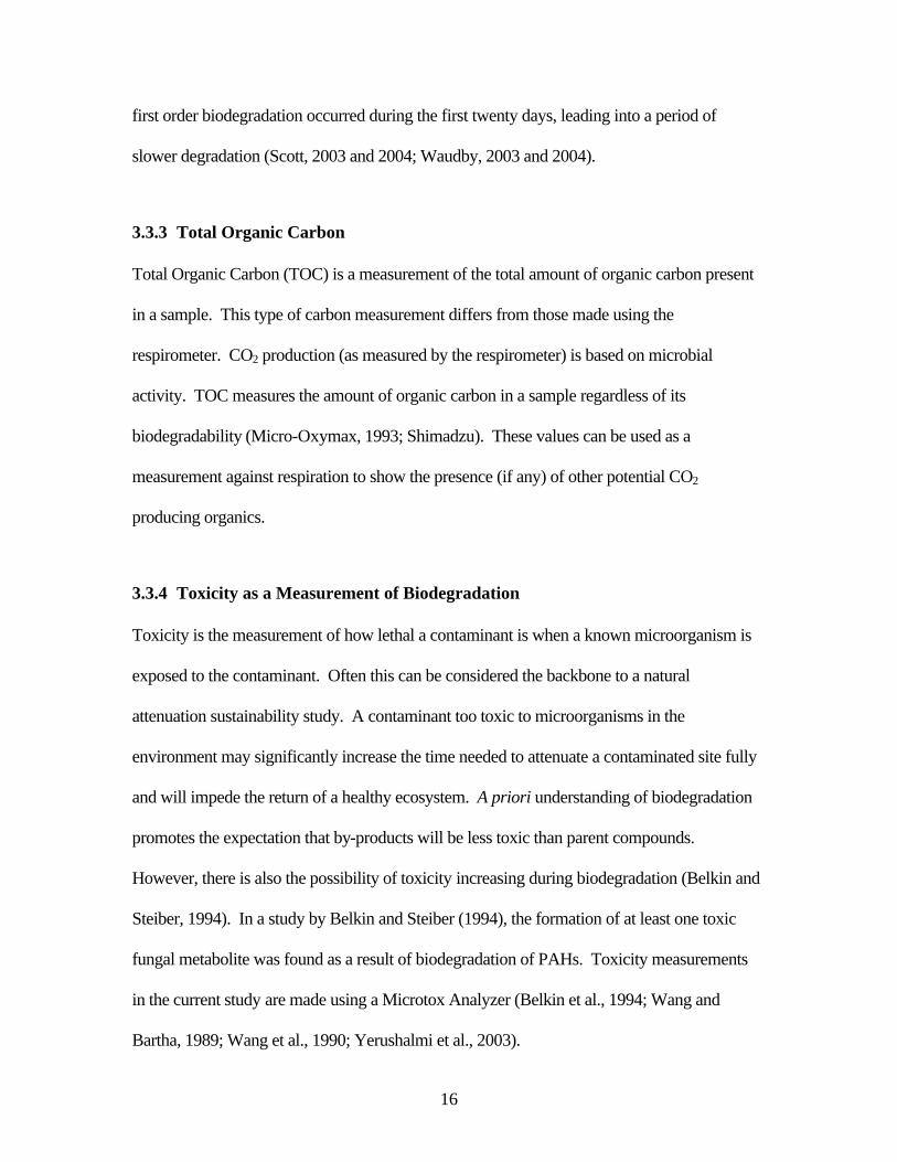
3.3.3 Total Organic Carbon
Total Organic Carbon (TOC) is a measurement of the total amount of organic carbon present
in a sample. This type of carbon measurement differs from those made using the
respirometer. CO2 production (as measured by the respirometer) is based on microbial
activity. TOC measures the amount of organic carbon in a sample regardless of its
biodegradability (Micro-Oxymax, 1993; Shimadzu). These values can be used as a
measurement against respiration to show the presence (if any) of other potential CO2
producing organics.
3.3.4 Toxicity as a Measurement of Biodegradation
Toxicity is the measurement of how lethal a contaminant is when a known microorganism is
exposed to the contaminant. Often this can be considered the backbone to a natural
attenuation sustainability study. A contaminant too toxic to microorganisms in the
environment may significantly increase the time needed to attenuate a contaminated site fully
and will impede the return of a healthy ecosystem. A priori understanding of biodegradation
promotes the expectation that by-products will be less toxic than parent compounds.
However, there is also the possibility of toxicity increasing during biodegradation (Belkin and
Steiber, 1994). In a study by Belkin and Steiber (1994), the formation of at least one toxic
fungal metabolite was found as a result of biodegradation of PAHs. Toxicity measurements
in the current study are made using a Microtox Analyzer (Belkin et al., 1994; Wang and
Bartha, 1989; Wang et al., 1990; Yerushalmi et al., 2003).
17
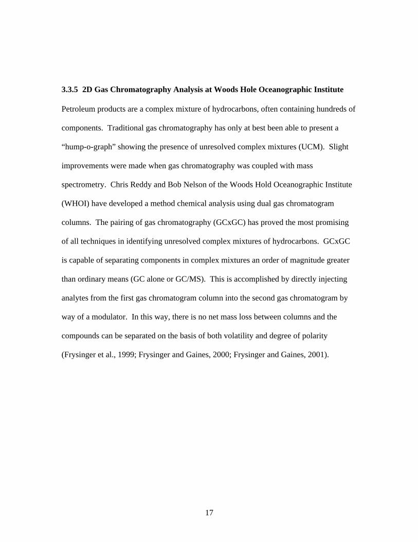
3.3.5 2D Gas Chromatography Analysis at Woods Hole Oceanographic Institute
Petroleum products are a complex mixture of hydrocarbons, often containing hundreds of
components. Traditional gas chromatography has only at best been able to present a
“hump-o-graph” showing the presence of unresolved complex mixtures (UCM). Slight
improvements were made when gas chromatography was coupled with mass
spectrometry. Chris Reddy and Bob Nelson of the Woods Hold Oceanographic Institute
(WHOI) have developed a method chemical analysis using dual gas chromatogram
columns. The pairing of gas chromatography (GCxGC) has proved the most promising
of all techniques in identifying unresolved complex mixtures of hydrocarbons. GCxGC
is capable of separating components in complex mixtures an order of magnitude greater
than ordinary means (GC alone or GC/MS). This is accomplished by directly injecting
analytes from the first gas chromatogram column into the second gas chromatogram by
way of a modulator. In this way, there is no net mass loss between columns and the
compounds can be separated on the basis of both volatility and degree of polarity
(Frysinger et al., 1999; Frysinger and Gaines, 2000; Frysinger and Gaines, 2001).
18
CHAPTER 4
MATERIALS AND METHODS
4.1 Groundwater Samples
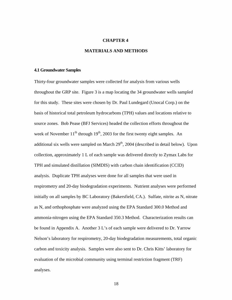
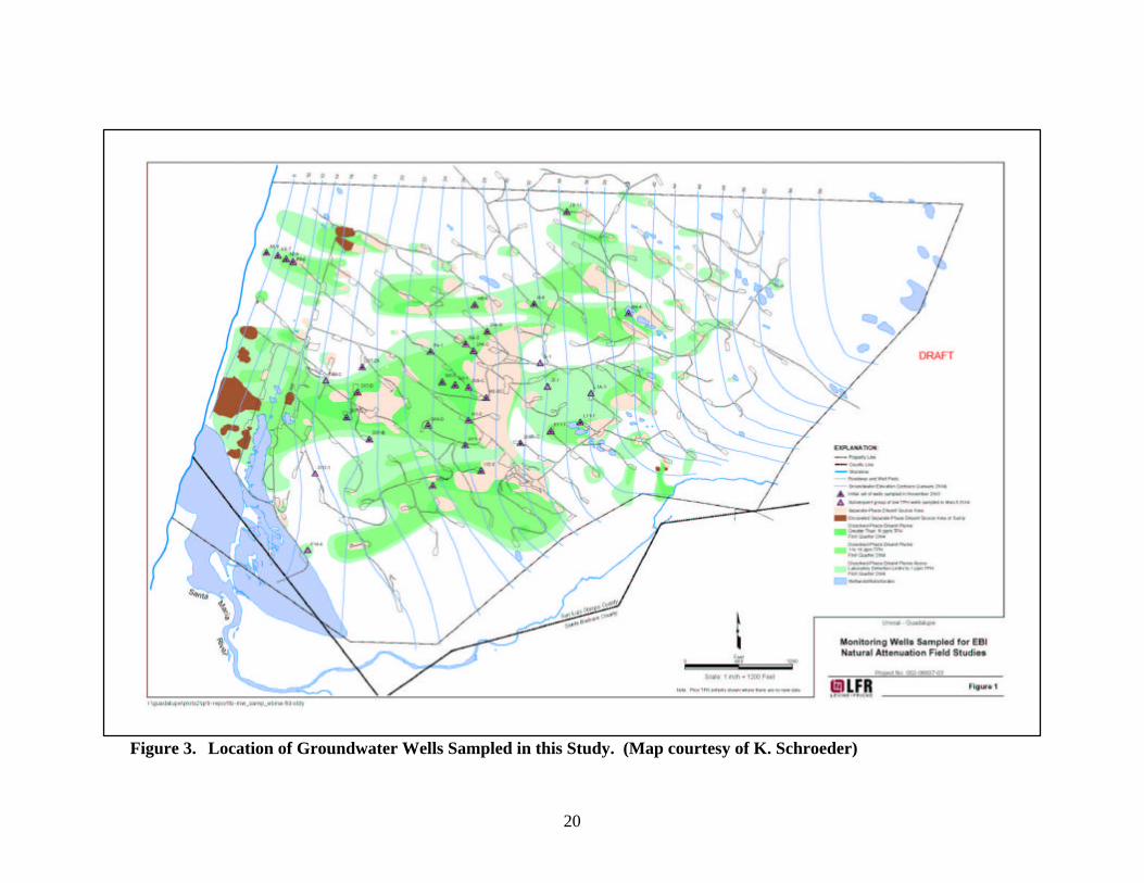
Thirty-four groundwater samples were collected for analysis from various wells
throughout the GRP site. Figure 3 is a map locating the 34 groundwater wells sampled
for this study. These sites were chosen by Dr. Paul Lundegard (Unocal Corp.) on the
basis of historical total petroleum hydrocarbons (TPH) values and locations relative to
source zones. Bob Pease (BFJ Services) headed the collection efforts throughout the
week of November 11th through 19th, 2003 for the first twenty eight samples. An
additional six wells were sampled on March 29th, 2004 (described in detail below). Upon
collection, approximately 1 L of each sample was delivered directly to Zymax Labs for
TPH and simulated distillation (SIMDIS) with carbon chain identification (CCID)
analysis. Duplicate TPH analyses were done for all samples that were used in
respirometry and 20-day biodegradation experiments. Nutrient analyses were performed
initially on all samples by BC Laboratory (Bakersfield, CA.). Sulfate, nitrite as N, nitrate
as N, and orthophosphate were analyzed using the EPA Standard 300.0 Method and
ammonia-nitrogen using the EPA Standard 350.3 Method. Characterization results can
be found in Appendix A. Another 3 L’s of each sample were delivered to Dr. Yarrow
Nelson’s laboratory for respirometry, 20-day biodegradation measurements, total organic
carbon and toxicity analysis. Samples were also sent to Dr. Chris Kitts’ laboratory for
evaluation of the microbial community using terminal restriction fragment (TRF)
analyses.
19
For fifteen of the initial set of wells all parameters were analyzed. The second batch of
thirteen wells was analyzed for all parameters except respirometry and 20-day biodegradation.
The third set of six samples was added to the study to provide samples with lower TPH
concentrations. These samples were extracted from GRP site wells known to have low TPH
levels (< 2 mg/L). Analyses of these samples were identical to Subset 1, with the exception of
respirometry. Subset 3 was the last batch of samples analyzed and was not restricted by time.
Therefore, Subset 3 samples were allowed to run for a full 20-day period on the respirometer.
All samples used are listed in Table 1.
20
Figure 3. Location of Groundwater Wells Sampled in this Study. (Map courtesy of K. Schroeder)
21
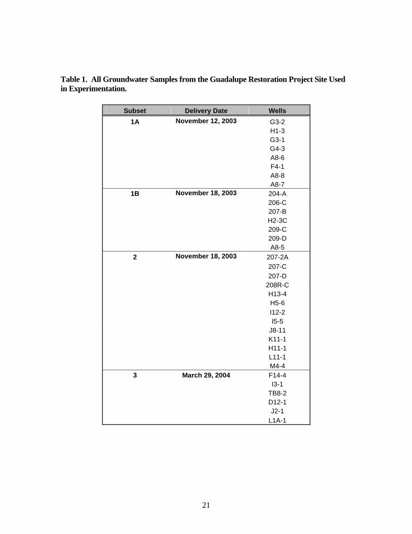
Table 1. All Groundwater Samples from the Guadalupe Restoration Project Site Used in Experimentation.
Subset Delivery Date Wells
1A November 12, 2003 G3-2 H1-3 G3-1 G4-3 A8-6 F4-1 A8-8 A8-7
1B November 18, 2003 204-A 206-C 207-B H2-3C 209-C 209-D A8-5 2 November 18, 2003 207-2A
207-C 207-D 208R-C H13-4 H5-6 I12-2 I5-5 J8-11 K11-1 H11-1 L11-1 M4-4
3 March 29, 2004 F14-4 I3-1 TB8-2 D12-1 J2-1 L1A-1

22
4.2 Respirometry Experiments
Respirometry was used to measure CO2 production for sample Subsets 1 and 3. Subset 1
was run for six days, while Subset 3 was run for twenty days. The variation in time was
due to time restrictions. A review of the experiments can be seen below.
4.2.1 Respirometry Methods
Microorganism respiration was measured using a Micro-Oxymax open cell respirometer
(Columbus Instruments, Columbus, Ohio). Open cell systems are able to supply fresh air
to experiments which undergo biological and chemical processes. Components of the
system include a sample pump, sample dryer column packed with magnesium
percholorate (Mg(ClO4)2), infrared sensor, expansion interface (expandable to 10
sampling ports), condensing air dryer, and an air drying column (for ambient air)
containing CaSO4 (see Figure 4). A Columbus Micro Systems compatible IBM computer
connects to the respirometer and utilizes version 6.0 hardware components and version
6.06d and 6.09b upgraded software. CO2 production is measured using a single beam,
non-dispersive infrared CO2/CH4 sensor with a range of 0.0 to 1 %.
23
Figure 4. Respirometer components. Left: Sample pump, sample dryer column, and infrared sensor. Right: Expansion interface, condensing air dryer, waterbath, and temperature-controlled water recirculator.
Six experiments were run on the respirometer. The first experiment ran without
complications. However, problems were encountered while running the second
experiment. After consultation with the manufacturer, the sample port was shipped to
Columbus Instruments, Inc. for repair. No further complications were encountered after
the sample port was returned.
4.2.2 Respirometry Sample Preparation for Subset 1
At the time of experimentation nine test ports (out of ten) were functioning on the
respirometer. Thus, two batches of eight (Subset 1A) then seven (Subset 1B) samples were
run. A deionized water blank was run with each batch to provide a control. To accommodate
for these batched tests, Unocal spread out the delivery of both batches by one week.
24
CO2 production was monitored for a period of six days for each experiment for Subset 1.
Each sample port was connected to a two-liter glass media bottle with 2 liters of diluent-
contaminated groundwater sample. To keep the samples well oxygenated and promote
microbial degradation, the bottles were continuously stirred by magnetic stirrers. To
match field conditions, the samples were kept in a water bath regulated at a constant
temperature of 19°C. No nutrients were added to any of the samples during measurement
of respiration. Figure 5 shows the sample set-up for the respirometer runs.
Figure 5. Respirometry sample set-up for groundwater samples.
25
4.2.3 Respirometry Sample Preparation for Subset 3
Ideally, continuous respirometry would be run over the entire biodegradation period of
twenty days, but due to time constraints the samples in Subset 1 were only run for six
days. Continuous respirometry for Subset 3 was run for a full twenty days so that the
TPH loss in twenty days could be correlated with CO2 production.
For Subset 3, the respirometer was restarted after every 6 day period for three
consecutive runs. These runs were followed by the remaining period of two days. All
other set up conditions for Subset 3 were identical to Subset 1.
4.3 Total Organic Carbon (TOC) Measurement
TOC measurements were made to identify the presence of organic carbon. This method
varies from the respirometer by measuring all organic carbon, rather than focusing on
microbial production alone. Sample preparation was the same for all Subsets.
4.3.1 TOC Methods
TOC measurements were made using a Shimadzu TOC-5000A analyzer, as seen in
Figure 6. Inorganic carbon (HCO3- and CO3
2-) is removed from samples by adding pH=2
deionized water (using HCl) to the sample to acidify all inorganics. All initial CO2 is
then purged from the sample using nitrogen gas. Organic carbon is then measured by
thermally oxidizing all organic carbon to CO2 and then measuring the CO2 production by
non-dispersive infra-red analysis. All samples were run against a calibration curve of
pH=2 diluted samples of 1, 5, 10, and 20 mg/L of glucose standard. Each sample is
26
placed under a sampling port and allowed to run for two minutes performing a rotation of
sparging, measuring and washing. The final step of washing readies the sampling port
for the next measurement.
Midway through experimentation the inline sparger stopped functioning. Manual
sparging was then used by sparging each sample with an aquarium pump for one minute.
Figure 6. Shimadzu TOC-5000A analyzer. During inactivity, the sample port sits in a mixture of pH=2 deionized water. Insert: Photograph of the analyzer main menu.
27
4.3.2 TOC Sample Preparation
Each test sample was a combination of 5 mL of pH=2 deionized water and 5 mL of
groundwater sample. Diluting the samples gave TOC readings which were half of the
original concentration. Measurements were multiplied by two before recording in the
results section. TOC was measured for all samples in duplicate.
4.4 Toxicity Experiments
Toxicity is the measurement of how lethal a contaminant is to a known organism. For
these experiments, all toxicity measurements were made using the Microtox® method
which measures toxicity to the bioluminescent bacteria Vibrio Fisheri (bioluminescent
bacteria).
4.4.1 Toxicity Methods
Toxicity measurements were made using the Microtox 500 Analyzer by Strategic
Diagnostics, Inc. (Newark, DE). The use of this analyzer has been approved as a
regulatory test for the estimation of toxicity for oil well drilling sump fluids by the
Alberta Energy and Utilities Board (AZUR, 2004). All reagents, test solutions, and the
MicrotoxOmni software were also provided by Strategic Diagnostics, Inc. This analyzer
determines toxicity for a series of sample dilutions and interpolates to find the effective
concentration where 50% of the bioluminescent test bacteria are killed. This value is
termed an EC50. It is important to remember a high EC50 value represents a low toxicity
and vice versa.
28
To ensure proper operation, a 100 mg/L phenol solution standard was tested occasionally.
According to manufacturers, the standard should result in an EC50 of between 13 to 26
mg/L.
4.4.2 Microtox® Sample Preparation
2.5 mL of each sample was transferred to a vial for analysis. Dilutions were made in
accordance to the “Basic Test” and performed manually in test vials set within the
analyzer (Figure 7). The Basic Test was performed in accordance to the methods
outlined by Strategic Diagnostics, Inc. and can be seen in Appendix C. Tests were
performed on all subsets (including initial and 20 day biodegradation for Subset 1 and 3)
and run in duplicate.
Figure 7. Microtox 500 Analyzer by Strategic Diagnostics, Inc. setup. Insert: Close-up of test vials used for sample dilution.
29
4.5 Total Petroleum Hydrocarbon (TPH) Analysis
TPH concentrations were determined using gas chromatography by Zymax Labs in
accordance with EPA standards. Initial samples collected from monitoring wells at the
GRP site by BFJ Services scientists were taken directly to Zymax Labs for analyses.
Twenty day biodegraded samples were collected by EBI scientists and shipped directly to
Zymax Labs for analyses. Samples were kept at a temperature of 4°C until analyses were
performed.
TPH analyses were performed by gas chromatography with mass spectrophotometry
detection (GC/MS). Samples are first extracted into methylene chloride (MCl) using
EPA Method 3510. After extraction, analyses are performed using an amended State of
California EPA Method 8015. TPH is then measured against diluent standards over an
analytical range of C10-C40.
4.6 Twenty Day Biodegradation Rate Analysis
To quantify biodegradation rates, TPH measurements were made after twenty days
of incubation. These measurements were made for Subsets 1 and 3. Subset 1 was
constantly stirred and incubated for fourteen days (after six days in the respirometer)
in an incubator at 19ºC (Figure 8). Subset 3 was constantly stirred and kept at a
constant temperature of 19ºC in the waterbath recirculator attached to the
respirometer apparatus. No nutrients or inoculum were added to any of the samples
for the biodegradation experiments. All samples were analyzed in duplicate by
30
Zymax Labs using EPA standardized gas chromatography tests. TOC and
Microtox® toxicity were measured in duplicate at the end of twenty days.
Figure 8. 14 day biodegradation period for Subset 1. Samples were stirred and kept refrigerated at a constant temperature of 19°C.
31
CHAPTER 5
RESULTS AND DISCUSSION
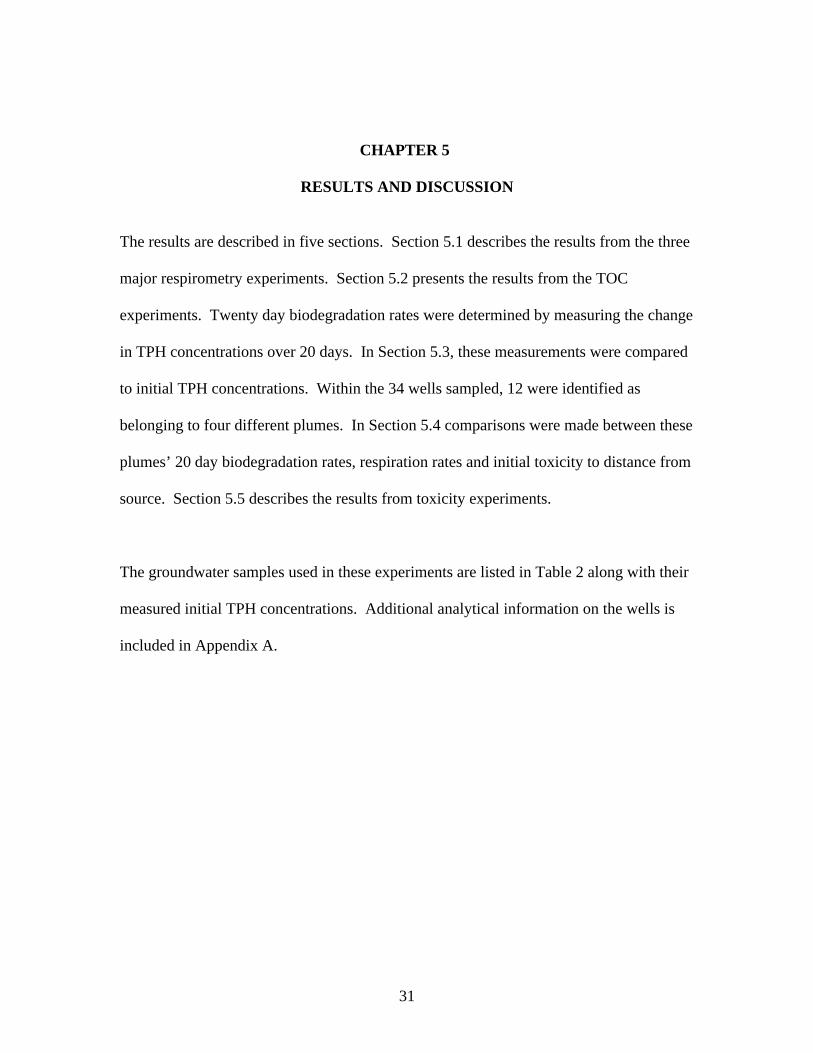
The results are described in five sections. Section 5.1 describes the results from the three
major respirometry experiments. Section 5.2 presents the results from the TOC
experiments. Twenty day biodegradation rates were determined by measuring the change
in TPH concentrations over 20 days. In Section 5.3, these measurements were compared
to initial TPH concentrations. Within the 34 wells sampled, 12 were identified as
belonging to four different plumes. In Section 5.4 comparisons were made between these
plumes’ 20 day biodegradation rates, respiration rates and initial toxicity to distance from
source. Section 5.5 describes the results from toxicity experiments.
The groundwater samples used in these experiments are listed in Table 2 along with their
measured initial TPH concentrations. Additional analytical information on the wells is
included in Appendix A.
32
Table 2. Initial TPH concentrations for all groundwater samples, as reported by Zymax Labs (detection limit = < 100 ug/L). For comparison, deionized water registered as non-detect for all carbon chain lengths using the same Zymax analytical methods.
Initial TPH Concentration
(ug/L)
Sample Rep. 1 Rep. 2 Ave. Std. Dev.
Subset 1A A8-6 4800 1900 3350 2050.6 (8) A8-7 2300 1900 2100 282.8
A8-8 3200 3200 3200 0.0 F4-1 1300 1400 1350 70.7 G3-1 10000 11000 10500 707.1 G3-2 12000 13000 12500 707.1 G4-3 7600 6500 7050 777.8 H1-3 9800 11000 10400 848.5 Subset 1B 204-A 2200 2400 2300 141.4
(7) 206-C 3800 4700 4250 636.4 207-B 400 510 455 77.8 H2-3C 11000 13000 12000 1414.2 209-C 13000 16000 14500 2121.3 209-D 8700 7200 7950 1060.7 A8-5 9000 36000 22500 19091.9
Subset 2 207-2A 2800 (13) 207-C 9900
207-D 9300 208R-C ND H13-4 11000 H5-6 4200 I12-2 11000 I5-5 2500 J8-11 7400 K11-1 5500 H11-1 3000 L11-1 8500 M4-4 12000
Subset 3 F14-4 220 180 200 28.3 (6) I3-1 N/A N/A 49 N/A
TB8-2 2800 2700 2750 70.7 D12-1 N/A N/A 49 N/A J2-1 420 420 420 0.0 L1A-1 N/A N/A 49 N/A
33
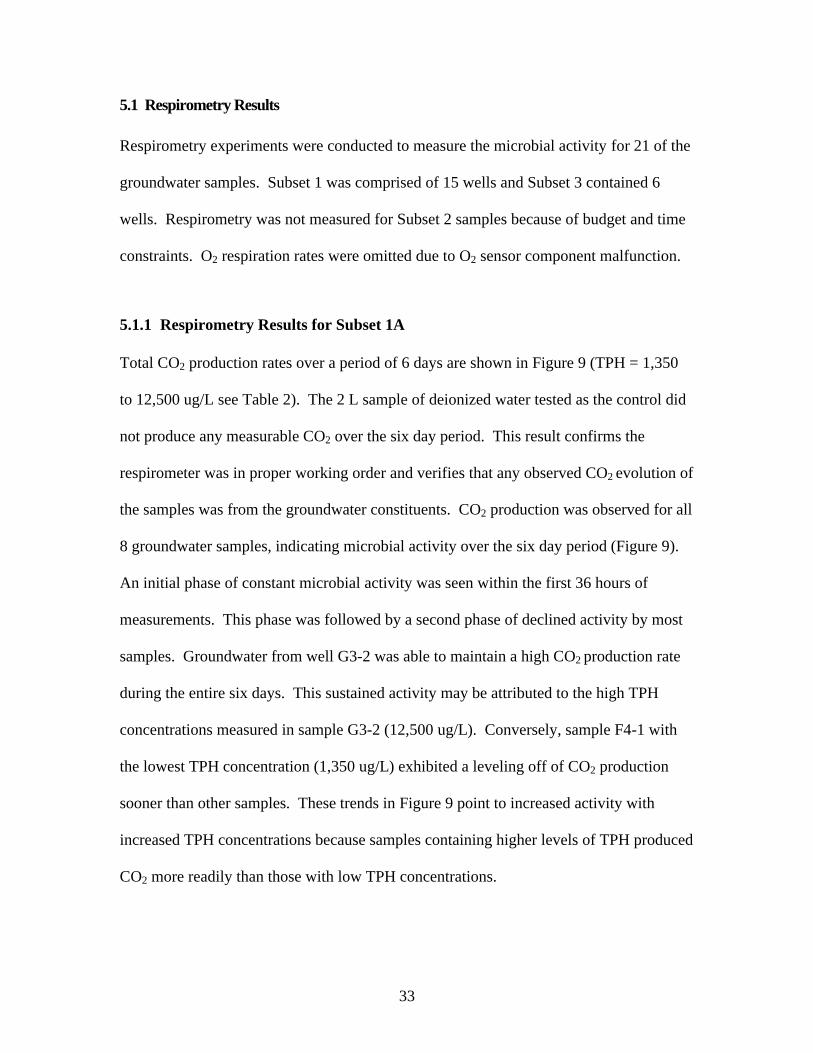
5.1 Respirometry Results
Respirometry experiments were conducted to measure the microbial activity for 21 of the
groundwater samples. Subset 1 was comprised of 15 wells and Subset 3 contained 6
wells. Respirometry was not measured for Subset 2 samples because of budget and time
constraints. O2 respiration rates were omitted due to O2 sensor component malfunction.
5.1.1 Respirometry Results for Subset 1A
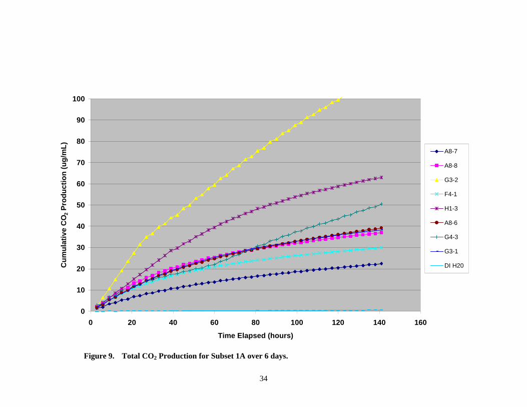
Total CO2 production rates over a period of 6 days are shown in Figure 9 (TPH = 1,350
to 12,500 ug/L see Table 2). The 2 L sample of deionized water tested as the control did
not produce any measurable CO2 over the six day period. This result confirms the
respirometer was in proper working order and verifies that any observed CO2 evolution of
the samples was from the groundwater constituents. CO2 production was observed for all
8 groundwater samples, indicating microbial activity over the six day period (Figure 9).
An initial phase of constant microbial activity was seen within the first 36 hours of
measurements. This phase was followed by a second phase of declined activity by most
samples. Groundwater from well G3-2 was able to maintain a high CO2 production rate
during the entire six days. This sustained activity may be attributed to the high TPH
concentrations measured in sample G3-2 (12,500 ug/L). Conversely, sample F4-1 with
the lowest TPH concentration (1,350 ug/L) exhibited a leveling off of CO2 production
sooner than other samples. These trends in Figure 9 point to increased activity with
increased TPH concentrations because samples containing higher levels of TPH produced
CO2 more readily than those with low TPH concentrations.
34
Figure 9. Total CO2 Production for Subset 1A over 6 days.
0
10
20
30
40
50
60
70
80
90
100
0 20 40 60 80 100 120 140 160
Time Elapsed (hours)
Cu
mu
lati
ve C
O2
Pro
du
ctio
n (
ug
/mL
)
A8-7
A8-8
G3-2
F4-1
H1-3
A8-6
G4-3
G3-1
DI H20
35
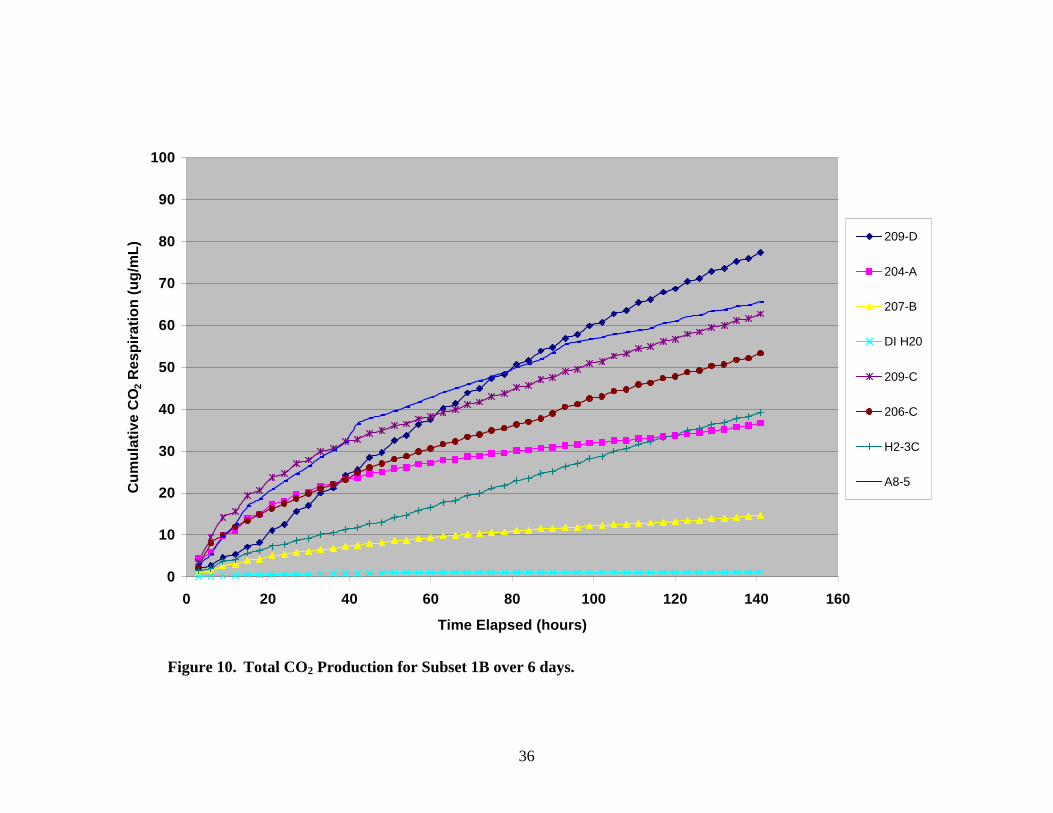
5.1.2 Respirometry Results for Subset 1B
Subset 1B grouped 7 groundwater samples with TPH concentrations ranging from 455 to
22,500 ug/L (see Table 2). Total CO2 production rates over a period of 6 days are shown
in Figure 10. The deionized control sample again did not produce any measurable CO2
over the six day period. Similar trends from Subset 1A were observed in Subset 1B.
Constant-rate microbial activity was observed for the first 36 hours of measurements
followed by a period of decreased activity (Figure 10). The trends of high CO2
respiration with high TPH concentrations from Subset 1A were again seen in this subset,
with the exception of samples 209-D and H2-3C. Sample 209-D exhibited a high level of
CO2 inconsistent with its relatively low initial TPH concentration. Conversely, sample
H2-3C exhibited a low level of CO2 given the samples high initial TPH concentration.
36
Figure 10. Total CO2 Production for Subset 1B over 6 days.
0
10
20
30
40
50
60
70
80
90
100
0 20 40 60 80 100 120 140 160
Time Elapsed (hours)
Cu
mu
lati
ve C
O2
Res
pir
atio
n (
ug
/mL
) 209-D
204-A
207-B
DI H20
209-C
206-C
H2-3C
A8-5
37
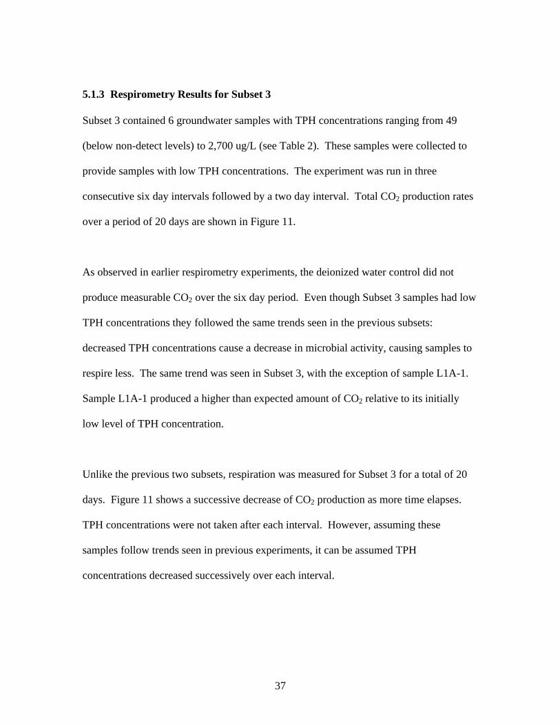
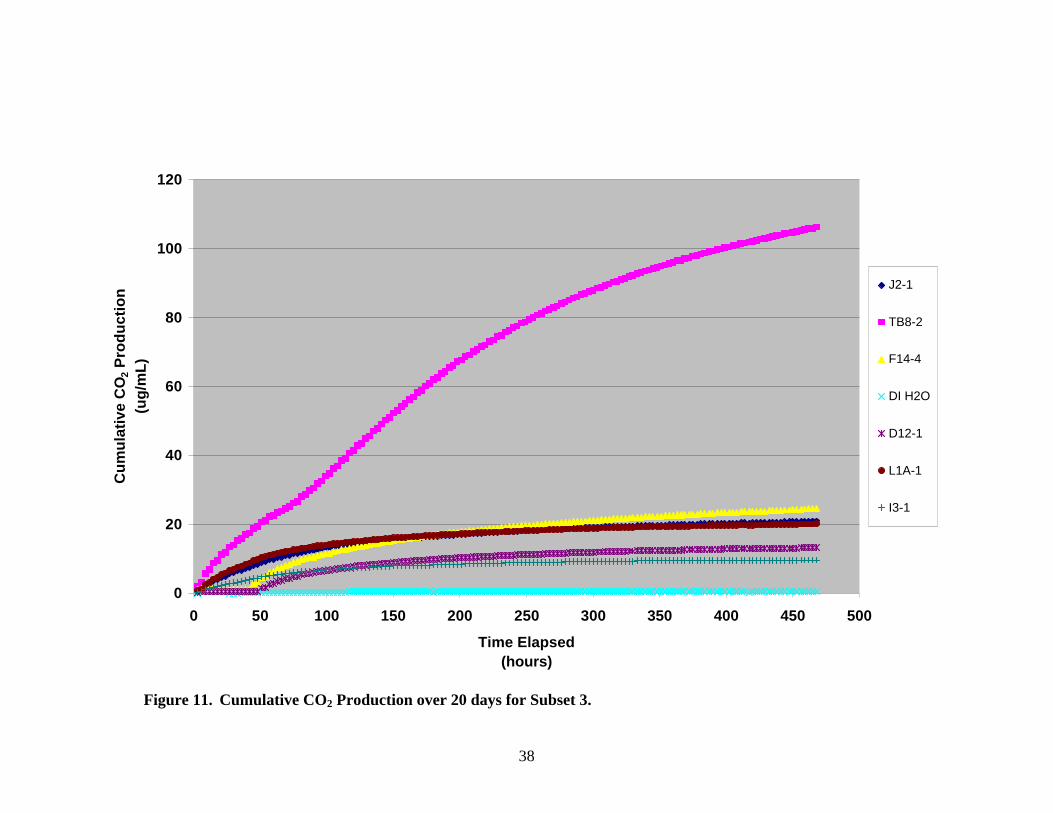
5.1.3 Respirometry Results for Subset 3
Subset 3 contained 6 groundwater samples with TPH concentrations ranging from 49
(below non-detect levels) to 2,700 ug/L (see Table 2). These samples were collected to
provide samples with low TPH concentrations. The experiment was run in three
consecutive six day intervals followed by a two day interval. Total CO2 production rates
over a period of 20 days are shown in Figure 11.
As observed in earlier respirometry experiments, the deionized water control did not
produce measurable CO2 over the six day period. Even though Subset 3 samples had low
TPH concentrations they followed the same trends seen in the previous subsets:
decreased TPH concentrations cause a decrease in microbial activity, causing samples to
respire less. The same trend was seen in Subset 3, with the exception of sample L1A-1.
Sample L1A-1 produced a higher than expected amount of CO2 relative to its initially
low level of TPH concentration.
Unlike the previous two subsets, respiration was measured for Subset 3 for a total of 20
days. Figure 11 shows a successive decrease of CO2 production as more time elapses.
TPH concentrations were not taken after each interval. However, assuming these
samples follow trends seen in previous experiments, it can be assumed TPH
concentrations decreased successively over each interval.
38
Figure 11. Cumulative CO2 Production over 20 days for Subset 3.
0
20
40
60
80
100
120
0 50 100 150 200 250 300 350 400 450 500
Time Elapsed(hours)
Cu
mu
lati
ve C
O2
Pro
du
ctio
n(u
g/m
L)
J2-1
TB8-2
F14-4
DI H2O
D12-1
L1A-1
I3-1
39
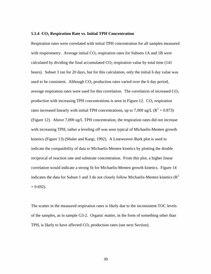
5.1.4 CO2 Respiration Rate vs. Initial TPH Concentration
Respiration rates were correlated with initial TPH concentration for all samples measured
with respirometry. Average initial CO2 respiration rates for Subsets 1A and 1B were
calculated by dividing the final accumulated CO2 respiration value by total time (141
hours). Subset 3 ran for 20 days, but for this calculation, only the initial 6 day value was
used to be consistent. Although CO2 production rates varied over the 6 day period,
average respiration rates were used for this correlation. The correlation of increased CO2
production with increasing TPH concentrations is seen in Figure 12. CO2 respiration
rates increased linearly with initial TPH concentrations, up to 7,000 ug/L (R2 = 0.873)
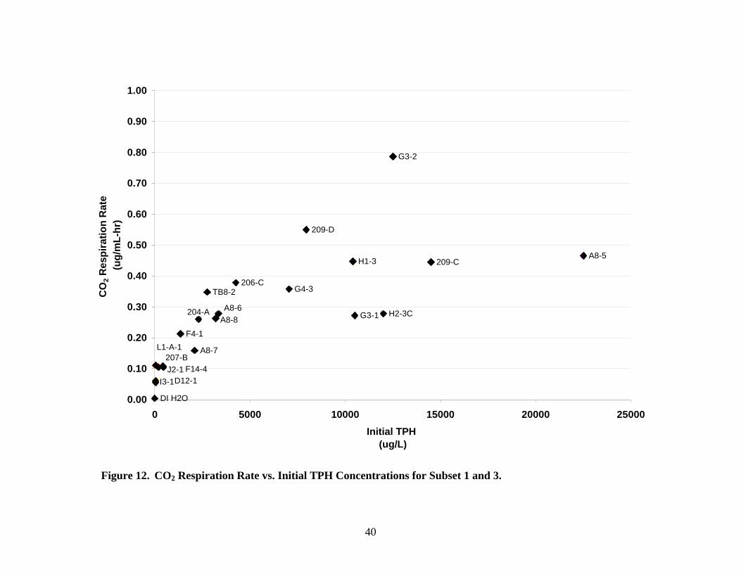
(Figure 12). Above 7,000 ug/L TPH concentration, the respiration rates did not increase
with increasing TPH, rather a leveling off was seen typical of Michaelis-Menten growth
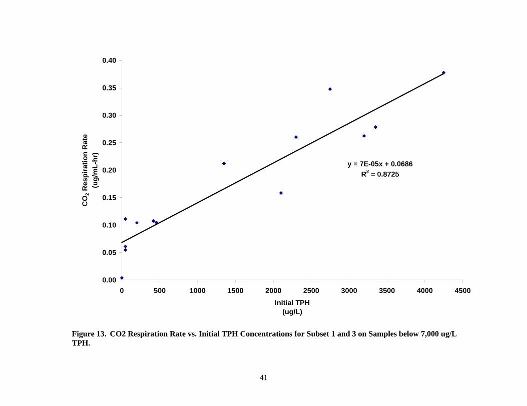
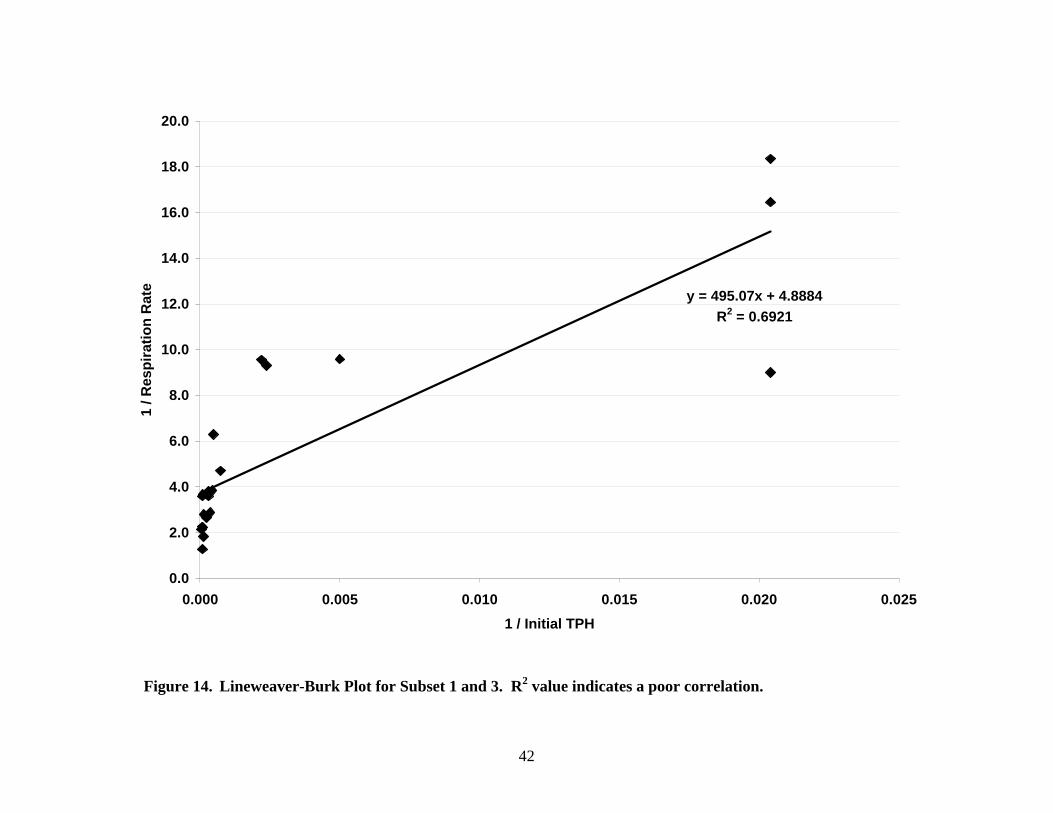
kinetics (Figure 13) (Shuler and Kargi, 1992). A Lineweaver-Burk plot is used to
indicate the compatibility of data to Michaelis-Menten kinetics by plotting the double
reciprocal of reaction rate and substrate concentration. From this plot, a higher linear
correlation would indicate a strong fit for Michaelis-Menten growth kinetics. Figure 14
indicates the data for Subset 1 and 3 do not closely follow Michaelis-Menten kinetics (R2
= 0.692).
The scatter in the measured respiration rates is likely due to the inconsistent TOC levels
of the samples, as in sample G3-2. Organic matter, in the form of something other than
TPH, is likely to have affected CO2 production rates (see next Section).
40
Figure 12. CO2 Respiration Rate vs. Initial TPH Concentrations for Subset 1 and 3.
206-C
A8-5209-C
H2-3C
209-D
A8-7
G3-2
F4-1
H1-3
G4-3
G3-1
DI H2O
TB8-2
204-A
207-B
A8-8A8-6
F14-4
I3-1D12-1J2-1
L1-A-1
0.00
0.10
0.20
0.30
0.40
0.50
0.60
0.70
0.80
0.90
1.00
0 5000 10000 15000 20000 25000
Initial TPH (ug/L)
CO
2 R
esp
irat
ion
Rat
e (u
g/m
L-h
r)
41
y = 7E-05x + 0.0686R2 = 0.8725
0.00
0.05
0.10
0.15
0.20
0.25
0.30
0.35
0.40
0 500 1000 1500 2000 2500 3000 3500 4000 4500
Initial TPH(ug/L)
CO
2 R
esp
irat
ion
Rat
e(u
g/m
L-h
r)
Figure 13. CO2 Respiration Rate vs. Initial TPH Concentrations for Subset 1 and 3 on Samples below 7,000 ug/L TPH.
42
Figure 14. Lineweaver-Burk Plot for Subset 1 and 3. R2 value indicates a poor correlation.
y = 495.07x + 4.8884R2 = 0.6921
0.0
2.0
4.0
6.0
8.0
10.0
12.0
14.0
16.0
18.0
20.0
0.000 0.005 0.010 0.015 0.020 0.025
1 / Initial TPH
1 / R
esp
irat
ion
Rat
e
43
5.2 TOC Results
TOC analysis was used to measure the total organic carbon present in all 34 groundwater
samples. This method varies from the respirometer by measuring all organic carbon,
rather than focusing on microbial production alone. Initial TOC concentrations of the
groundwater samples are tabulated in Table 3. TOC concentrations ranged from 13 to 42
mg organic carbon / L of sample.
Figure 15 identifies that a correlation between initial TOC versus initial TPH
concentrations does not exist (R2 = 0.156). This indicates groundwater samples vary in
natural organic matter content. It should also be noted that samples with very low TPH
concentrations exhibited a wide range of TOC concentrations from 10 to 35 mg/L.
TOC levels in the samples may have influenced respiration rates measured for some of
the samples. Sample 209-D contained high TOC levels (Table 3) which may have
contributed to a higher CO2 production rate (Figure 10). However, there was no
correlation observed between TOC levels and CO2 production rates (Figure 16).
44
Table 3. Initial TOC Results for all 34 Groundwater Samples.
Initial TOC Concentrations (mg/L)
Sample TPH
(ug/L) Rep. 1 Rep. 2 Ave. Std. Dev.
Subset 1A A8-6 3350 23.6 22.1 22.9 1.1 (8) A8-7 2100 26.6 24.8 25.7 1.2
A8-8 3200 19.9 18.3 19.1 1.1 F4-1 1350 13.6 12.6 13.1 0.7 G3-1 10500 35.8 34 35.0 1.3 G3-2 12500 42.3 39.3 40.8 2.1 G4-3 7050 22.3 19 20.7 2.3 H1-3 10400 23 22 22.5 0.7
Subset 1B 204-A 2300 13 14.3 13.6 0.9 (7) 206-C 4250 16 14 15.0 1.5
207-B 455 11.7 25 18.3 9.3 H2-3C 12000 31.9 29.8 30.8 1.5 209-C 14500 39.3 41.8 40.6 1.8 209-D 7950 30.1 28.6 29.4 1.1 A8-5 22500 23.7 24.9 24.3 0.8 Subset 2 207-2A 2800 13.2 14.5 13.9 0.9
(13) 207-C 9900 31.4 29.3 30.4 1.5 207-D 9300 27 25.9 26.4 0.7 208R-C ND 10.1 11 10.5 0.6 H13-4 11000 40.6 35.3 38.0 3.7 H5-6 4200 21.1 19 20.1 1.5 I12-2 11000 41.4 41.5 41.5 0.0 I5-5 2500 13.8 14.6 14.2 0.6 J8-11 7400 13.2 19.3 16.2 4.4 K11-1 5500 39.5 42 40.8 1.8 H11-1 3000 14.4 15 14.7 0.4 L11-1 8500 30.9 28.1 29.5 2.0 M4-4 12000 23.2 22.5 22.9 0.5 Subset 3 F14-4 200 36 30.1 33.0 4.2
(6) I3-1 49 43.7 29 36.4 10.3 TB8-2 2750 26.9 24.4 25.6 1.7 D12-1 49 37.9 25.6 31.8 8.7 J2-1 420 36.5 20.8 28.7 11.1 L1A-1 49 24.2 26.9 25.6 1.9
45
Figure 15. Initial TOC Concentrations vs. Initial TPH Concentrations for all 34 Groundwater Samples.
A8-6
A8-8
F4-1
G3-1
G4-3H1-3
206-C
207-B
H2-3C
209-C
A8-5
207-2A
207-C
207-D
208R-C
H13-4
H5-6
I12-2
J8-11
K11-1
L11-1
M4-4
F14-4
I3-1
TB8-2
D12-1
J2-1
L1A-1
G3-2
A8-7
204-A
209-D
I5-5
H11-1
y = 0.0007x + 21.557R2 = 0.1558
0
5
10
15
20
25
30
35
40
45
0 5000 10000 15000 20000 25000
Initial TPH(ug/L)
Init
ial T
OC
(mg
/L)

46
Figure 16. CO2 Respiration Rate vs. Initial TOC Concentration for all 34 Groundwater Wells.
0.00
0.10
0.20
0.30
0.40
0.50
0.60
0.70
0.80
0.90
0 5 10 15 20 25 30 35 40 45
Initial TOC Concentration(mg/L)
CO
2 R
esp
irat
ion
Rat
e(u
g/m
L-h
r)
47
5.3 20-Day Biodegradation Rates
The most direct measure of active biodegradation is measurement of TPH changes over
time. For 21 wells (Subsets 1 and 3) TPH analyses were made in duplicate by Zymax
Labs initially and again after 20 days of biodegradation in the lab at 19°C.
Biodegradation rates were calculated by dividing the change in TPH concentration (initial
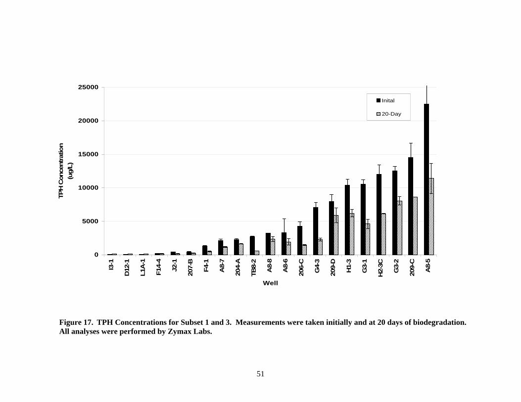
minus 20 day) over the 20 day time interval (Table 4). Figure 17 outlines the degradation
of TPH for those two time intervals for Subset 1 and 3. Significant reductions in TPH
concentration were observed for all samples with measurable initial TPH concentrations.
Table 4. 20 Day TPH Biodegradation Rates for Subset 1 and 3. All TPH concentrations were reported by Zymax Labs.
Subset 1 and 3
Sample
Initial TPH (ug/L)
Final TPH (20 day)
(ug/L)
20 Day Biodeg. Rate (ug/L-day)
Subset 1A A8-6 3350 1950 70 (8) A8-7 2100 1150 48
A8-8 3200 2350 43 F4-1 1350 520 42 G3-1 10500 4600 295 G3-2 12500 8050 223 G4-3 7050 2250 240 H1-3 10400 6200 210
Subset 1B 204-A 2300 1650 33 (7) 206-C 4250 1450 140
207-B 455 230 11 H2-3C 12000 6150 293 209-C 14500 8600 295 209-D 7950 5900 103 A8-5 22500 11400 555
Subset 3 F14-4 200 165 2 (6) I3-1 NA NA NA
TB8-2 2750 575 109 D12-1 NA NA NA J2-1 420 160 13 L1A-1 NA NA NA
48
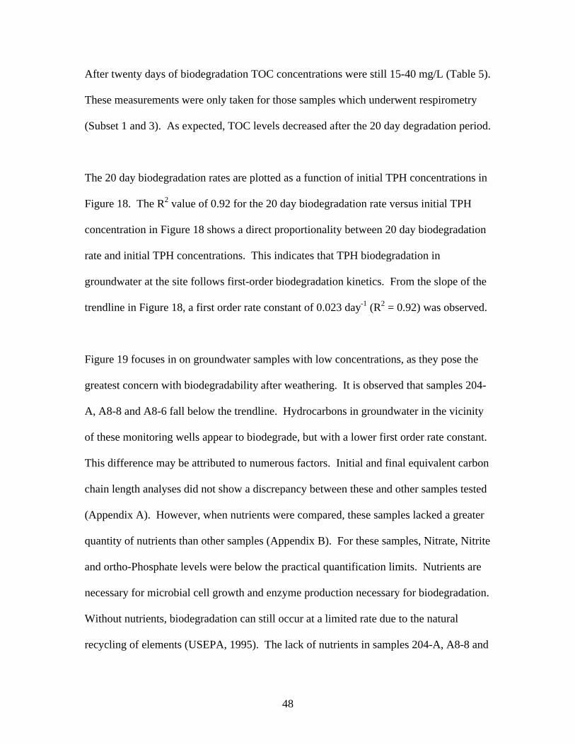
After twenty days of biodegradation TOC concentrations were still 15-40 mg/L (Table 5).
These measurements were only taken for those samples which underwent respirometry
(Subset 1 and 3). As expected, TOC levels decreased after the 20 day degradation period.
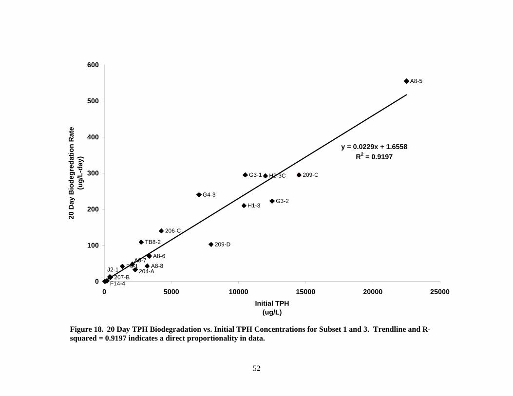
The 20 day biodegradation rates are plotted as a function of initial TPH concentrations in
Figure 18. The R2 value of 0.92 for the 20 day biodegradation rate versus initial TPH
concentration in Figure 18 shows a direct proportionality between 20 day biodegradation
rate and initial TPH concentrations. This indicates that TPH biodegradation in
groundwater at the site follows first-order biodegradation kinetics. From the slope of the
trendline in Figure 18, a first order rate constant of 0.023 day-1 (R2 = 0.92) was observed.
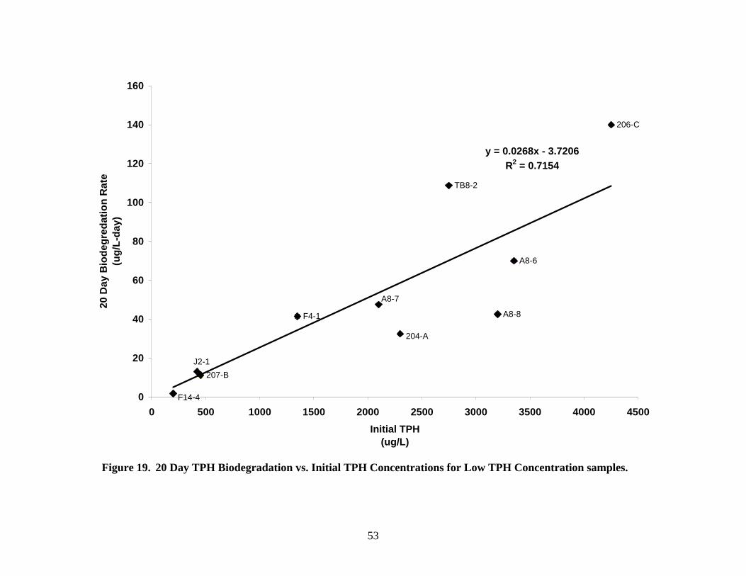
Figure 19 focuses in on groundwater samples with low concentrations, as they pose the
greatest concern with biodegradability after weathering. It is observed that samples 204-
A, A8-8 and A8-6 fall below the trendline. Hydrocarbons in groundwater in the vicinity
of these monitoring wells appear to biodegrade, but with a lower first order rate constant.
This difference may be attributed to numerous factors. Initial and final equivalent carbon
chain length analyses did not show a discrepancy between these and other samples tested
(Appendix A). However, when nutrients were compared, these samples lacked a greater
quantity of nutrients than other samples (Appendix B). For these samples, Nitrate, Nitrite
and ortho-Phosphate levels were below the practical quantification limits. Nutrients are
necessary for microbial cell growth and enzyme production necessary for biodegradation.
Without nutrients, biodegradation can still occur at a limited rate due to the natural
recycling of elements (USEPA, 1995). The lack of nutrients in samples 204-A, A8-8 and
49
A8-6 may have led to the lower rates of biodegradation observed. Overall, samples with
low TPH concentrations (first order rate constant = 0.027 day-1) followed similar first
order kinetics as high TPH samples which indicates that biodegradability of
hydrocarbons is not hindered by chemical changes between high and low TPH
concentrations. Sample F14-4 also showed slightly lower TPH biodegradation than
expected from the first order plot. From Appendix B, this sample also contained low
levels of Nitrate, Nitrite and ortho-Phosphate.
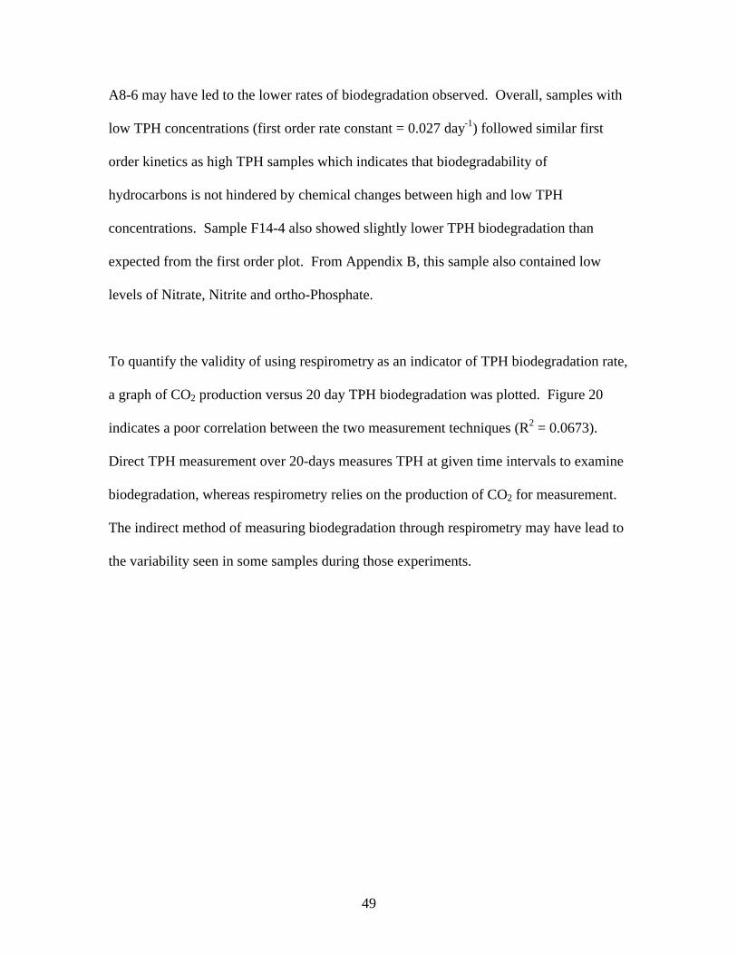
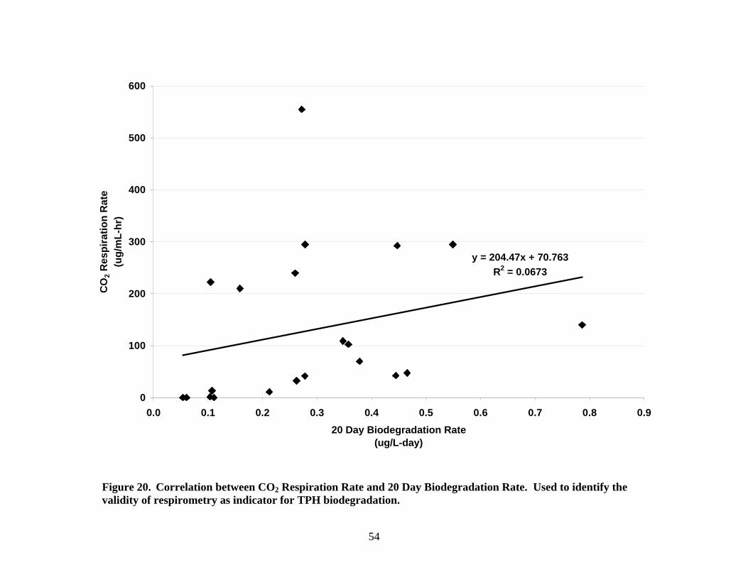
To quantify the validity of using respirometry as an indicator of TPH biodegradation rate,
a graph of CO2 production versus 20 day TPH biodegradation was plotted. Figure 20
indicates a poor correlation between the two measurement techniques (R2 = 0.0673).
Direct TPH measurement over 20-days measures TPH at given time intervals to examine
biodegradation, whereas respirometry relies on the production of CO2 for measurement.
The indirect method of measuring biodegradation through respirometry may have lead to
the variability seen in some samples during those experiments.

50
Table 5. Twenty Day TOC Results for Subset 1 and 3.
After 20 Day Biodegradation
Final TOC Concentration (mg/L)
Sample TPH Rep. 1 Rep. 2 Ave. Std. Dev.
Subset 1A A8-6 1950 17.19 17.996 17.6 0.6 (8) A8-7 1150 14.956 12.948 14.0 1.4
A8-8 2350 17.648 13.436 15.5 3.0 F4-1 520 10.148 11.71 10.9 1.1 G3-1 4600 24.86 26.82 25.8 1.4 G3-2 8050 39.4 40.4 39.9 0.7 G4-3 2250 14.304 14.68 14.5 0.3 H1-3 6200 19.618 20.36 20.0 0.5
Subset 1B 204-A 1650 13.854 12.26 13.1 1.1 (7) 206-C 1450 14.548 16.632 15.6 1.5
207-B 230 10.056 10.862 10.5 0.6 H2-3C 6150 28.6 27.28 27.9 0.9 209-C 8600 32.9 32.74 32.8 0.1 209-D 5900 20.72 20.92 20.8 0.1 A8-5 11400 24.12 24.58 24.4 0.3
Subset 3 F14-4 14 17.786 20.84 19.3 2.2 (6) I3-1 99 21.86 11.222 16.5 7.5
TB8-2 14 19.13 18.06 18.6 0.8 D12-1 99 25.7 15.632 20.7 7.1 J2-1 16 27.14 7.746 17.4 13.7 L1A-1 99 25.66 10.26 18.0 10.9
51
Figure 17. TPH Concentrations for Subset 1 and 3. Measurements were taken initially and at 20 days of biodegradation. All analyses were performed by Zymax Labs.
0
5000
10000
15000
20000
25000
I3-1
D12
-1
L1A
-1
F14
-4
J2-1
207-
B
F4-
1
A8-
7
204-
A
TB
8-2
A8-
8
A8-
6
206-
C
G4-
3
209-
D
H1-
3
G3-
1
H2-
3C
G3-
2
209-
C
A8-
5
Well
TP
H C
once
ntr
atio
n(u
g/L
)
Inital
20-Day
52
Figure 18. 20 Day TPH Biodegradation vs. Initial TPH Concentrations for Subset 1 and 3. Trendline and R-squared = 0.9197 indicates a direct proportionality in data.
A8-6
A8-8F4-1
G3-1
G3-2G4-3
H1-3
206-C
207-B
H2-3C 209-C
209-D
A8-5
TB8-2
A8-7
204-A
F14-4
J2-1
y = 0.0229x + 1.6558R2 = 0.9197
0
100
200
300
400
500
600
0 5000 10000 15000 20000 25000
Initial TPH(ug/L)
20 D
ay B
iod
egre
dat
ion
Rat
e(u
g/L
-day
)
53
Figure 19. 20 Day TPH Biodegradation vs. Initial TPH Concentrations for Low TPH Concentration samples.
A8-6
A8-8F4-1
206-C
207-B
TB8-2
A8-7
204-A
F14-4
J2-1
y = 0.0268x - 3.7206R2 = 0.7154
0
20
40
60
80
100
120
140
160
0 500 1000 1500 2000 2500 3000 3500 4000 4500
Initial TPH(ug/L)
20 D
ay B
iod
egre
dat
ion
Rat
e(u
g/L
-day
)
54
Figure 20. Correlation between CO2 Respiration Rate and 20 Day Biodegradation Rate. Used to identify the validity of respirometry as indicator for TPH biodegradation.
y = 204.47x + 70.763R2 = 0.0673
0
100
200
300
400
500
600
0.0 0.1 0.2 0.3 0.4 0.5 0.6 0.7 0.8 0.9
20 Day Biodegradation Rate(ug/L-day)
CO
2 R
esp
irat
ion
Rat
e(u
g/m
L-h
r)
55
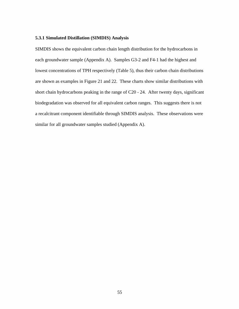
5.3.1 Simulated Distillation (SIMDIS) Analysis
SIMDIS shows the equivalent carbon chain length distribution for the hydrocarbons in
each groundwater sample (Appendix A). Samples G3-2 and F4-1 had the highest and
lowest concentrations of TPH respectively (Table 5), thus their carbon chain distributions
are shown as examples in Figure 21 and 22. These charts show similar distributions with
short chain hydrocarbons peaking in the range of C20 - 24. After twenty days, significant
biodegradation was observed for all equivalent carbon ranges. This suggests there is not
a recalcitrant component identifiable through SIMDIS analysis. These observations were
similar for all groundwater samples studied (Appendix A).
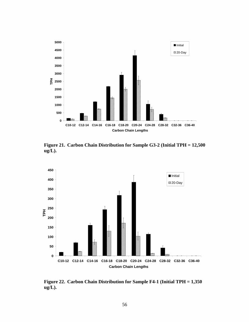
56
0
500
1000
1500
2000
2500
3000
3500
4000
4500
5000
C10-12 C12-14 C14-16 C16-18 C18-20 C20-24 C24-28 C28-32 C32-36 C36-40
Carbon Chain Lengths
TP
H
Initial
20-Day
Figure 21. Carbon Chain Distribution for Sample G3-2 (Initial TPH = 12,500 ug/L).
0
50
100
150
200
250
300
350
400
450
C10-12 C12-14 C14-16 C16-18 C18-20 C20-24 C24-28 C28-32 C32-36 C36-40
Carbon Chain Lengths
TP
H
Initial
20-Day
Figure 22. Carbon Chain Distribution for Sample F4-1 (Initial TPH = 1,350 ug/L).
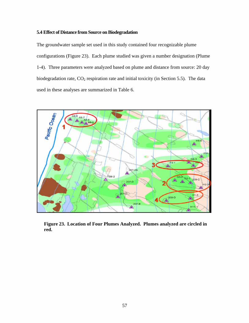
57
5.4 Effect of Distance from Source on Biodegradation
The groundwater sample set used in this study contained four recognizable plume
configurations (Figure 23). Each plume studied was given a number designation (Plume
1-4). Three parameters were analyzed based on plume and distance from source: 20 day
biodegradation rate, CO2 respiration rate and initial toxicity (in Section 5.5). The data
used in these analyses are summarized in Table 6.
Figure 23. Location of Four Plumes Analyzed. Plumes analyzed are circled in red.
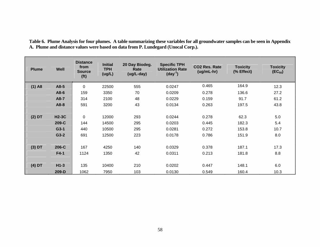
58
Table 6. Plume Analysis for four plumes. A table summarizing these variables for all groundwater samples can be seen in Appendix A. Plume and distance values were based on data from P. Lundegard (Unocal Corp.).
Plume Well
Distance from
Source (ft)
Initial TPH
(ug/L)
20 Day Biodeg. Rate
(ug/L-day)
Specific TPH Utilization Rate
(day-1)
CO2 Res. Rate (ug/mL-hr)
Toxicity (% Effect)
Toxicity (EC50)
(1) A8 A8-5 0 22500 555 0.0247 0.465 164.9 12.3 A8-6 159 3350 70 0.0209 0.278 136.6 27.2 A8-7 314 2100 48 0.0229 0.159 91.7 61.2 A8-8 591 3200 43 0.0134 0.263 197.5 43.8
(2) DT H2-3C 0 12000 293 0.0244 0.278 62.3 5.0 209-C 144 14500 295 0.0203 0.445 182.3 5.4 G3-1 440 10500 295 0.0281 0.272 153.8 10.7 G3-2 691 12500 223 0.0178 0.786 151.9 8.0
(3) DT 206-C 167 4250 140 0.0329 0.378 187.1 17.3 F4-1 1124 1350 42 0.0311 0.213 181.8 8.8
(4) DT H1-3 135 10400 210 0.0202 0.447 148.1 6.0
209-D 1062 7950 103 0.0130 0.549 160.4 10.3
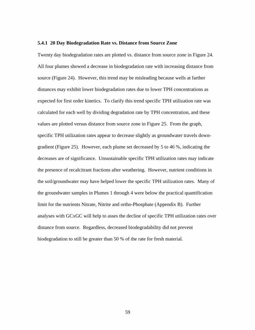
59
5.4.1 20 Day Biodegradation Rate vs. Distance from Source Zone
Twenty day biodegradation rates are plotted vs. distance from source zone in Figure 24.
All four plumes showed a decrease in biodegradation rate with increasing distance from
source (Figure 24). However, this trend may be misleading because wells at farther
distances may exhibit lower biodegradation rates due to lower TPH concentrations as
expected for first order kinetics. To clarify this trend specific TPH utilization rate was
calculated for each well by dividing degradation rate by TPH concentration, and these
values are plotted versus distance from source zone in Figure 25. From the graph,
specific TPH utilization rates appear to decrease slightly as groundwater travels down-
gradient (Figure 25). However, each plume set decreased by 5 to 46 %, indicating the
decreases are of significance. Unsustainable specific TPH utilization rates may indicate
the presence of recalcitrant fractions after weathering. However, nutrient conditions in
the soil/groundwater may have helped lower the specific TPH utilization rates. Many of
the groundwater samples in Plumes 1 through 4 were below the practical quantification
limit for the nutrients Nitrate, Nitrite and ortho-Phosphate (Appendix B). Further
analyses with GCxGC will help to asses the decline of specific TPH utilization rates over
distance from source. Regardless, decreased biodegradability did not prevent
biodegradation to still be greater than 50 % of the rate for fresh material.
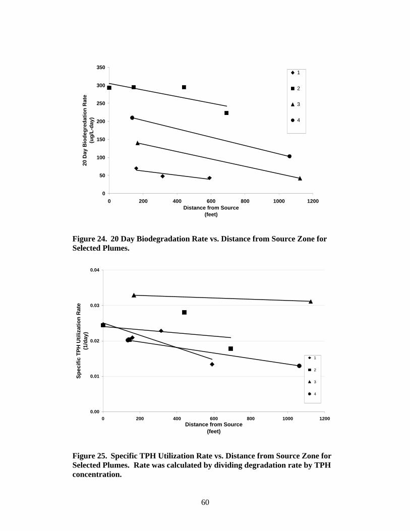
60
0
50
100
150
200
250
300
350
0 200 400 600 800 1000 1200Distance from Source
(feet)
20 D
ay B
iod
egre
dat
ion
Rat
e(u
g/L
-day
)
1
2
3
4
Lin
Figure 24. 20 Day Biodegradation Rate vs. Distance from Source Zone for Selected Plumes.
0.00
0.01
0.02
0.03
0.04
0 200 400 600 800 1000 1200Distance from Source
(feet)
Sp
ecif
ic T
PH
Uti
lizat
ion
Rat
e(1
/day
)
1
2
3
4
Figure 25. Specific TPH Utilization Rate vs. Distance from Source Zone for Selected Plumes. Rate was calculated by dividing degradation rate by TPH concentration.
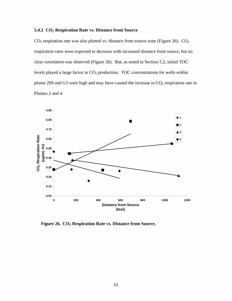
61
5.4.2 CO2 Respiration Rate vs. Distance from Source
CO2 respiration rate was also plotted vs. distance from source zone (Figure 26). CO2
respiration rates were expected to decrease with increased distance from source, but no
clear correlation was observed (Figure 26). But, as noted in Section 5.2, initial TOC
levels played a large factor in CO2 production. TOC concentrations for wells within
plume 209 and G3 were high and may have caused the increase in CO2 respiration rate in
Plumes 2 and 4.
0.00
0.10
0.20
0.30
0.40
0.50
0.60
0.70
0.80
0.90
0 200 400 600 800 1000 1200
Distance from Source(feet)
CO
2 R
esp
irat
ion
Rat
e(u
g/m
L-h
r)
1
2
3
4
Figure 26. CO2 Respiration Rate vs. Distance from Source.
62
5.5 Toxicity Results
Microtox® toxicity was measured for all 34 groundwater samples. Subset names have
been retained from the respirometry experiments. The Microtox® analyzer interpolates
the measured toxicity effect of a series of sample dilutions to find the effective
concentration where 50% of the bioluminescent test bacteria are killed. This value is
termed an EC50. EC50 values for the groundwater samples ranged from 5 to 100 % (Table
7). It is important to remember a high EC50 value represents a low toxicity and vice
versa. Samples with the result “No EC50” exhibited such a low toxicity that an EC50
could not be determined. EC50 decreases rapidly with increasing TPH concentration
indicating a strong increase in toxicity with increasing TPH concentration (Figure 27).
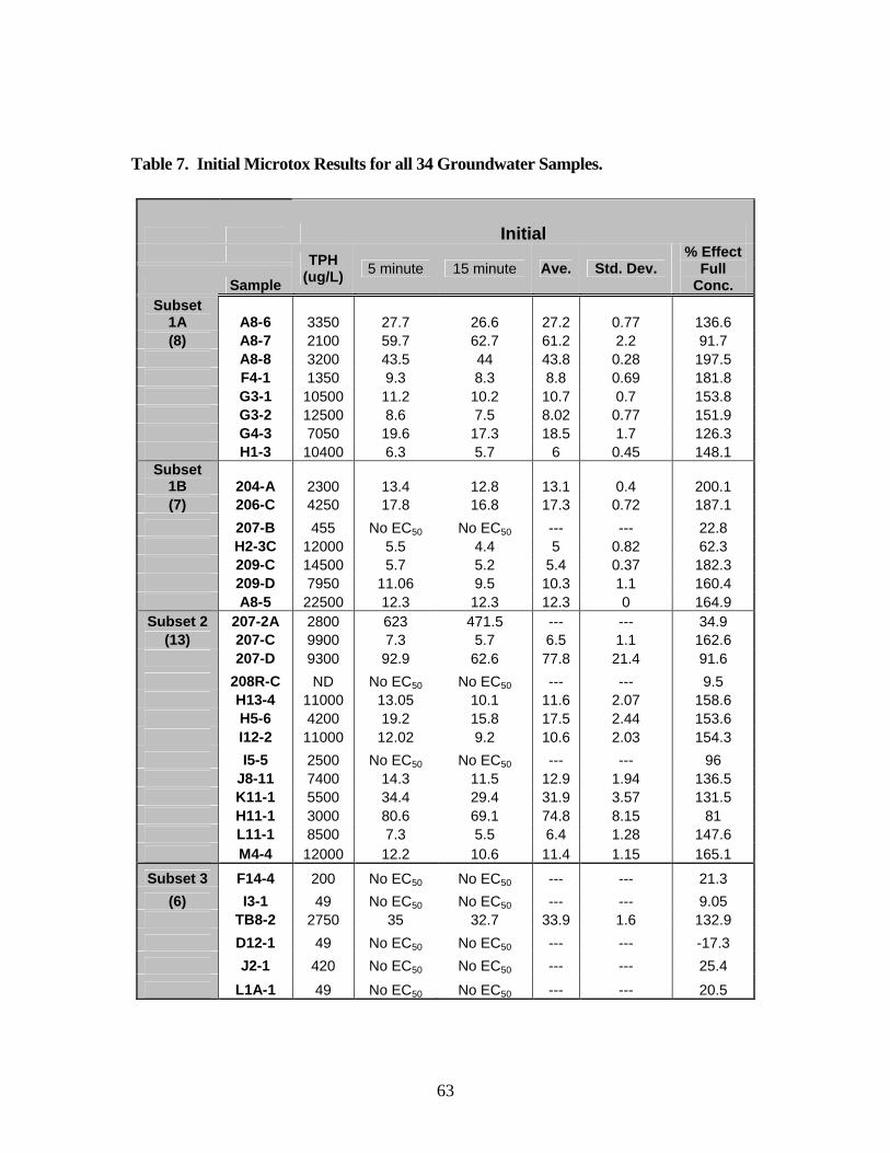
63
Table 7. Initial Microtox Results for all 34 Groundwater Samples.
Initial
Sample
TPH (ug/L) 5 minute 15 minute Ave. Std. Dev.
% Effect Full
Conc. Subset
1A A8-6 3350 27.7 26.6 27.2 0.77 136.6 (8) A8-7 2100 59.7 62.7 61.2 2.2 91.7
A8-8 3200 43.5 44 43.8 0.28 197.5 F4-1 1350 9.3 8.3 8.8 0.69 181.8 G3-1 10500 11.2 10.2 10.7 0.7 153.8 G3-2 12500 8.6 7.5 8.02 0.77 151.9 G4-3 7050 19.6 17.3 18.5 1.7 126.3 H1-3 10400 6.3 5.7 6 0.45 148.1
Subset 1B 204-A 2300 13.4 12.8 13.1 0.4 200.1 (7) 206-C 4250 17.8 16.8 17.3 0.72 187.1
207-B 455 No EC50 No EC50 --- --- 22.8 H2-3C 12000 5.5 4.4 5 0.82 62.3 209-C 14500 5.7 5.2 5.4 0.37 182.3 209-D 7950 11.06 9.5 10.3 1.1 160.4 A8-5 22500 12.3 12.3 12.3 0 164.9 Subset 2 207-2A 2800 623 471.5 --- --- 34.9
(13) 207-C 9900 7.3 5.7 6.5 1.1 162.6 207-D 9300 92.9 62.6 77.8 21.4 91.6
208R-C ND No EC50 No EC50 --- --- 9.5 H13-4 11000 13.05 10.1 11.6 2.07 158.6 H5-6 4200 19.2 15.8 17.5 2.44 153.6 I12-2 11000 12.02 9.2 10.6 2.03 154.3
I5-5 2500 No EC50 No EC50 --- --- 96 J8-11 7400 14.3 11.5 12.9 1.94 136.5 K11-1 5500 34.4 29.4 31.9 3.57 131.5 H11-1 3000 80.6 69.1 74.8 8.15 81 L11-1 8500 7.3 5.5 6.4 1.28 147.6 M4-4 12000 12.2 10.6 11.4 1.15 165.1
Subset 3 F14-4 200 No EC50 No EC50 --- --- 21.3
(6) I3-1 49 No EC50 No EC50 --- --- 9.05 TB8-2 2750 35 32.7 33.9 1.6 132.9
D12-1 49 No EC50 No EC50 --- --- -17.3
J2-1 420 No EC50 No EC50 --- --- 25.4
L1A-1 49 No EC50 No EC50 --- --- 20.5
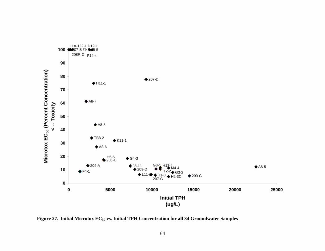
64
Figure 27. Initial Microtox EC50 vs. Initial TPH Concentration for all 34 Groundwater Samples
A8-6
A8-7
A8-8
F4-1 G3-2
G4-3
H1-3
204-A
206-C
H2-3C 209-C
209-DA8-5
207-D
I5-5
J8-11
K11-1
H11-1
L11-1
M4-4
TB8-2
G3-1
207-B
207-C
208R-C
H13-4
H5-6
I12-2
F14-4
I3-1D12-1J2-1L1A-1
0
10
20
30
40
50
60
70
80
90
100
0 5000 10000 15000 20000 25000
Initial TPH(ug/L)
Mic
roto
x E
C50
(P
erce
nt
Co
nce
ntr
atio
n)
< --
To
xici
ty
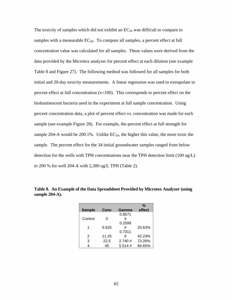
65
The toxicity of samples which did not exhibit an EC50 was difficult to compare to
samples with a measurable EC50. To compare all samples, a percent effect at full
concentration value was calculated for all samples. These values were derived from the
data provided by the Microtox analyzer for percent effect at each dilution (see example
Table 8 and Figure 27). The following method was followed for all samples for both
initial and 20-day toxicity measurements. A linear regression was used to extrapolate to
percent effect at full concentration (x=100). This corresponds to percent effect on the
bioluminescent bacteria used in the experiment at full sample concentration. Using
percent concentration data, a plot of percent effect vs. concentration was made for each
sample (see example Figure 28). For example, the percent effect at full strength for
sample 204-A would be 200.1%. Unlike EC50, the higher this value, the more toxic the
sample. The percent effect for the 34 initial groundwater samples ranged from below
detection for the wells with TPH concentrations near the TPH detection limit (100 ug/L)
to 200 % for well 204-A with 2,300 ug/L TPH (Table 2).
Table 8. An Example of the Data Spreadsheet Provided by Microtox Analyzer (using sample 204-A).
Sample Conc Gamma %
effect
Control 0 0.8571
#
1 5.625 0.2599
# 20.63%
2 11.25 0.7311
# 42.23% 3 22.5 2.740 # 73.26% 4 45 5.514 # 84.65%
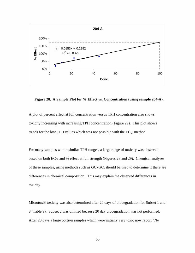
66
Figure 28. A Sample Plot for % Effect vs. Concentration (using sample 204-A).
A plot of percent effect at full concentration versus TPH concentration also shows
toxicity increasing with increasing TPH concentration (Figure 29). This plot shows
trends for the low TPH values which was not possible with the EC50 method.
For many samples within similar TPH ranges, a large range of toxicity was observed
based on both EC50 and % effect at full strength (Figures 28 and 29). Chemical analyses
of these samples, using methods such as GCxGC, should be used to determine if there are
differences in chemical composition. This may explain the observed differences in
toxicity.
Microtox® toxicity was also determined after 20 days of biodegradation for Subset 1 and
3 (Table 9). Subset 2 was omitted because 20 day biodegradation was not performed.
After 20 days a large portion samples which were initially very toxic now report “No
204-A
y = 0.0153x + 0.2292R2 = 0.8329
0%
50%
100%
150%
200%
0 20 40 60 80 100
Conc.
% E
ffec
t
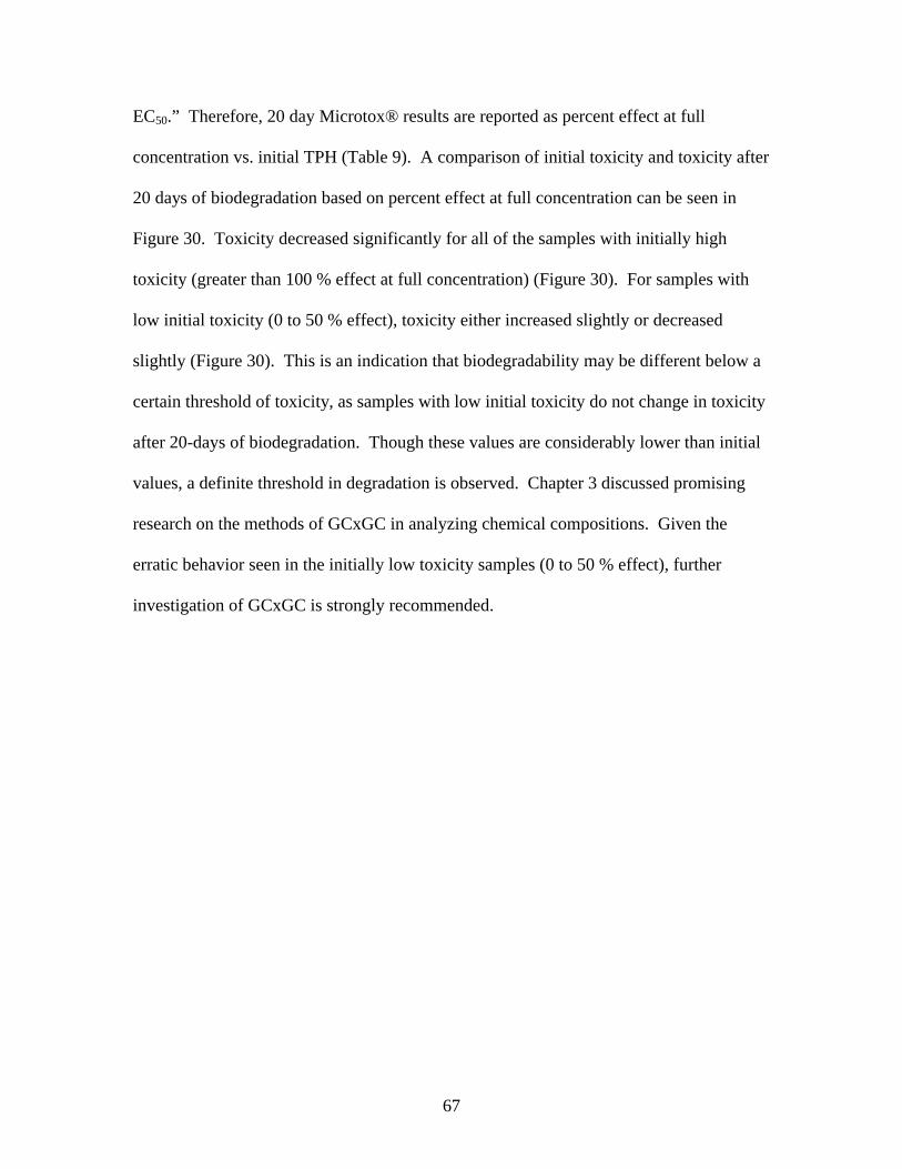
67
EC50.” Therefore, 20 day Microtox® results are reported as percent effect at full
concentration vs. initial TPH (Table 9). A comparison of initial toxicity and toxicity after
20 days of biodegradation based on percent effect at full concentration can be seen in
Figure 30. Toxicity decreased significantly for all of the samples with initially high
toxicity (greater than 100 % effect at full concentration) (Figure 30). For samples with
low initial toxicity (0 to 50 % effect), toxicity either increased slightly or decreased
slightly (Figure 30). This is an indication that biodegradability may be different below a
certain threshold of toxicity, as samples with low initial toxicity do not change in toxicity
after 20-days of biodegradation. Though these values are considerably lower than initial
values, a definite threshold in degradation is observed. Chapter 3 discussed promising
research on the methods of GCxGC in analyzing chemical compositions. Given the
erratic behavior seen in the initially low toxicity samples (0 to 50 % effect), further
investigation of GCxGC is strongly recommended.
68
Figure 29. Toxicity as measured by Initial % Effect at Full Concentration vs. Initial TPH Concentration for all groundwater samples.
A8-6
A8-8
F4-1
G3-2
G4-3
206-C
H2-3C
209-C
209-DA8-5
D12-1
207-2A
207-C
207-D
208R-C
H13-4H5-6 I12-2
I5-5
J8-11K11-1
H11-1
L11-1
M4-4
A8-7
G3-1
H1-3
204-A
207-BF14-4
I3-1
TB8-2
J2-1L1A-1
0
50
100
150
200
250
0 5000 10000 15000 20000 25000
Initial TPH Concentration(ug/L)
Init
ial %
Eff
ect
at F
ull
Co
nce
ntr
atio
nT
oxi
city
--
>
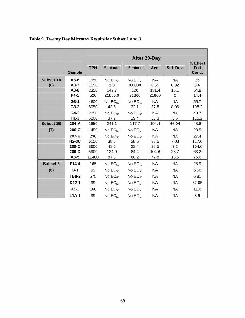
69
Table 9. Twenty Day Microtox Results for Subset 1 and 3.
After 20-Day
Sample TPH 5 minute 15 minute Ave. Std. Dev.
% Effect Full
Conc.
Subset 1A A8-6 1950 No EC50 No EC50 NA NA 26 (8) A8-7 1150 1.3 0.0008 0.65 0.92 9.6
A8-8 2350 142.7 120 131.4 16.1 54.8 F4-1 520 21860.0 21860 21860 0 14.4
G3-1 4600 No EC50 No EC50 NA NA 55.7 G3-2 8050 43.5 32.1 37.8 8.06 108.2
G4-3 2250 No EC50 No EC50 NA NA 40.7 H1-3 6200 37.2 29.4 33.3 5.6 115.2 Subset 1B 204-A 1650 241.1 147.7 194.4 66.04 48.6
(7) 206-C 1450 No EC50 No EC50 NA NA 28.5
207-B 230 No EC50 No EC50 NA NA 27.4 H2-3C 6150 38.5 28.6 33.5 7.03 117.6 209-C 8600 43.6 33.4 38.5 7.2 104.6 209-D 5900 124.9 84.4 104.6 28.7 63.2 A8-5 11400 87.3 68.2 77.8 13.5 76.6
Subset 3 F14-4 165 No EC50 No EC50 NA NA 28.9
(6) I3-1 99 No EC50 No EC50 NA NA 6.56
TB8-2 575 No EC50 No EC50 NA NA 6.81
D12-1 99 No EC50 No EC50 NA NA 32.05
J2-1 160 No EC50 No EC50 NA NA 11.6
L1A-1 99 No EC50 No EC50 NA NA 8.9
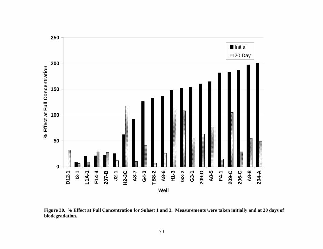
70
Figure 30. % Effect at Full Concentration for Subset 1 and 3. Measurements were taken initially and at 20 days of biodegradation.
0
50
100
150
200
250
D12
-1
I3-1
L1A
-1
F14
-4
207-
B
J2-1
H2-
3C
A8-
7
G4-
3
TB
8-2
A8-
6
H1-
3
G3-
2
G3-
1
209-
D
A8-
5
F4-
1
209-
C
206-
C
A8-
8
204-
A
Well
% E
ffec
t at
Fu
ll C
on
cen
trat
ion
Initial
20 Day
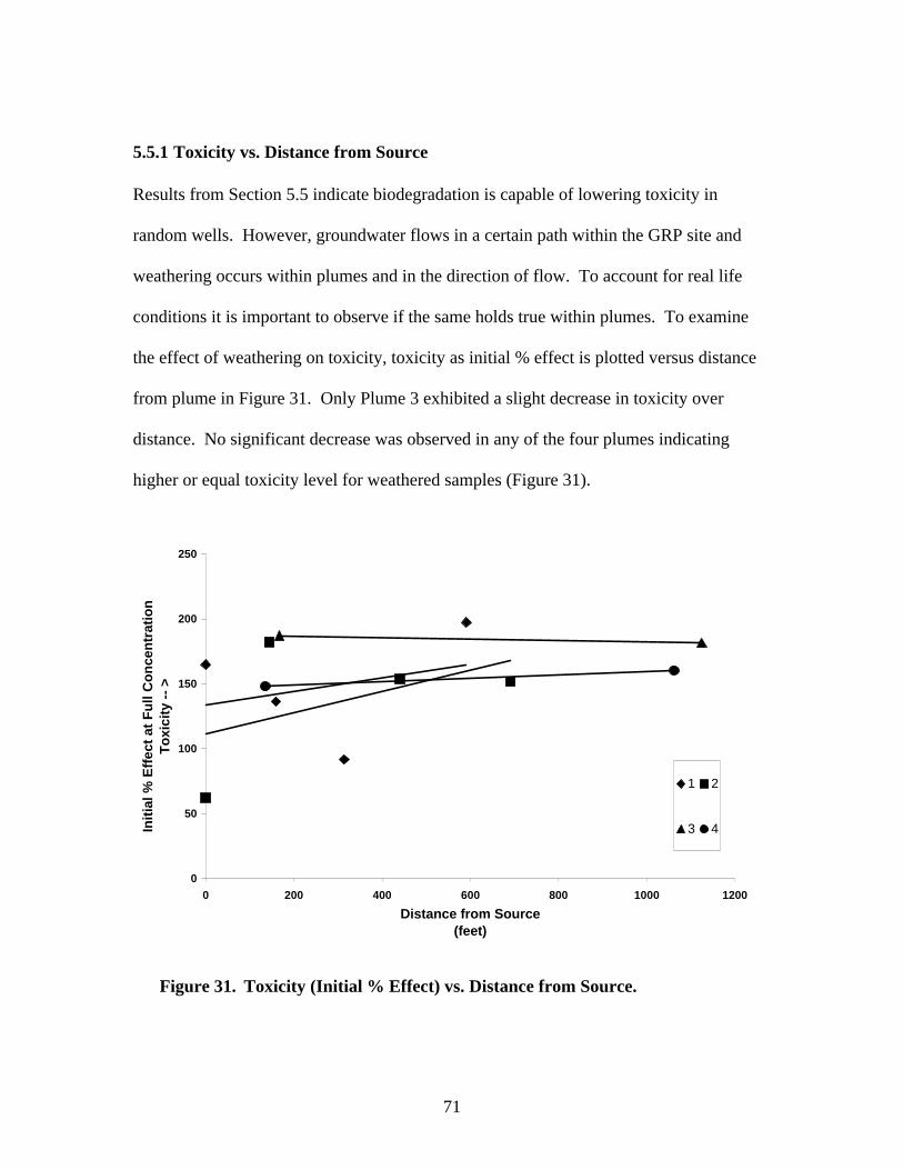
71
5.5.1 Toxicity vs. Distance from Source
Results from Section 5.5 indicate biodegradation is capable of lowering toxicity in
random wells. However, groundwater flows in a certain path within the GRP site and
weathering occurs within plumes and in the direction of flow. To account for real life
conditions it is important to observe if the same holds true within plumes. To examine
the effect of weathering on toxicity, toxicity as initial % effect is plotted versus distance
from plume in Figure 31. Only Plume 3 exhibited a slight decrease in toxicity over
distance. No significant decrease was observed in any of the four plumes indicating
higher or equal toxicity level for weathered samples (Figure 31).
0
50
100
150
200
250
0 200 400 600 800 1000 1200
Distance from Source(feet)
Init
ial %
Eff
ect
at F
ull
Co
nce
ntr
atio
nT
oxi
city
--
>
1 2
3 4
Figure 31. Toxicity (Initial % Effect) vs. Distance from Source.

72
This finding is significant such that it does not provide evidence that natural attenuation
is capable of reducing toxicity. However, laboratory studies are such that only certain
real life conditions are accounted for and Figure 31 was graphed based on many
assumptions. These assumptions include: 1) groundwater flow paths have not changed
since 2003 (print date of Figure 3), 2) no additional sources add contaminants to the
plumes, and 3) layers of free product are not present. A true account of real life
conditions would consider these situations. True field conditions may account for the
toxicity increases observed in Figure 31.
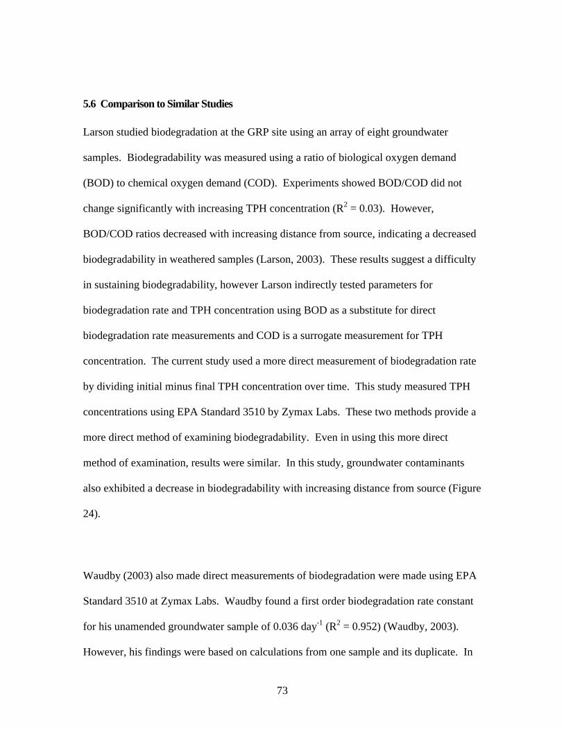
73
5.6 Comparison to Similar Studies
Larson studied biodegradation at the GRP site using an array of eight groundwater
samples. Biodegradability was measured using a ratio of biological oxygen demand
(BOD) to chemical oxygen demand (COD). Experiments showed BOD/COD did not
change significantly with increasing TPH concentration (R2 = 0.03). However,
BOD/COD ratios decreased with increasing distance from source, indicating a decreased
biodegradability in weathered samples (Larson, 2003). These results suggest a difficulty
in sustaining biodegradability, however Larson indirectly tested parameters for
biodegradation rate and TPH concentration using BOD as a substitute for direct
biodegradation rate measurements and COD is a surrogate measurement for TPH
concentration. The current study used a more direct measurement of biodegradation rate
by dividing initial minus final TPH concentration over time. This study measured TPH
concentrations using EPA Standard 3510 by Zymax Labs. These two methods provide a
more direct method of examining biodegradability. Even in using this more direct
method of examination, results were similar. In this study, groundwater contaminants
also exhibited a decrease in biodegradability with increasing distance from source (Figure
24).
Waudby (2003) also made direct measurements of biodegradation were made using EPA
Standard 3510 at Zymax Labs. Waudby found a first order biodegradation rate constant
for his unamended groundwater sample of 0.036 day-1 (R2 = 0.952) (Waudby, 2003).
However, his findings were based on calculations from one sample and its duplicate. In

74
this study a first order rate constant of 0.023 day-1 (R2 = 0.92) was calculated using a
greater array of groundwater samples. This method provides a more reliable estimate of
the first-order rate constant. It should be noted that first-order rate constants may be
lower in the field because of lower oxygen availability, lower nutrients and other similar
factors.
75
CHAPTER 6
CONCLUSIONS
Respirometry experiments indicated the presence of microbial activity in all thirty-four
groundwater wells sampled at the GRP site. An initial phase of greater microbial activity
was seen within the first 36 hours of measurements, followed by a second phase of
declined activity by most samples. This decline in degradation when samples
presumably contain lower (than initially measured) TPH concentrations was again seen in
correlations between CO2 respiration rate and initial TPH concentration.
TOC measurements indicated samples with lower TPH contained less organic matter,
leading to lower rates of CO2 production. However, TOC did not correlate very well
with TPH, suggesting the presence of natural organic matter other than TPH may
contribute to TOC.
Measured 20 day TPH biodegradation rates ranged from 2 to 550 ug/L-day and increased
with increasing TPH concentration. Biodegradation rate was directly proportional to
initial TPH concentration (R2 = 0.92) indicating TPH biodegradation in the groundwater
at the site follows first-order kinetics. The first order rate constant averaged over all
wells was 0.023 day-1 under these conditions. In comparison, Waudby (2003) found a
first order rate constant for his GRP groundwater sample of 0.036 day-1 (R2 = 0.952).
However, his findings were based on calculations from one sample and its duplicate.
Samples with very low TPH concentrations exhibited low biodegradation rates, but were
76
consistent with the first order rate constant for all samples. However, first order rate
constants decreased by 5 to 46 % for down gradient samples along four selected plumes.
This suggests that weathering decreases biodegradability of diluent, but biodegradation
continues at a reduced rate.
Another line of evidence for natural attenuation at this site is the observed decrease in
toxicity during biodegradation and with weathering. Toxicity studies show the site
capable of biodegrading the contaminants from high to lower toxicity levels. However,
this trend was present for only initially high TPH concentration samples (those greater
than 100 % effect at full concentration). Samples with low initial toxicity (0 to 50 %
effect) exhibited a slight decrease or, in some instances, an increase in toxicity. These
findings indicate a difficulty in reducing the toxicity of samples below a certain threshold
of toxicity.
Laboratory tests indicate all groundwater samples are able to biodegrade to a level of low
TPH. However, tests also indicated groundwater with low initial TPH concentrations did
not significantly change in toxicity over the 20-day period. Though these values are
considerably lower than initial values, a definite asymptote in degradation is seen. After
the period of most active biodegradation (twenty days) slight amounts of both TPH and
toxicity remained. Now, the classic question of “how low is low enough” comes into
play, leaving regulators to decide on appropriate endpoints for natural attenuation. The
toxicity endpoints that may be required by regulatory agencies are unknown to the
experimenter. But, if the values present in this data set meet the requirements, the use of

77
natural attenuation may still be feasible regardless of residual TPH concentrations or
toxicity.
78
CHAPTER 7
RECOMMENDATIONS
The following are recommendations included for further investigations of the correlation
of dissolved-phase diluent biodegradability and toxicity with weathering at the GRP site.
• Determine the source of the toxicity threshold exhibited after a twenty day period
in initially low TPH concentration samples.
• Follow up on GCxGC analysis at Woods Hold Oceanographic Institute. These
methods may be the key to determining chemical composition effects on
biodegradation and toxicity.
• Examine biodegradation with electron acceptors other than oxygen.
• Compare TPH toxicity levels of these samples to those required by regulatory
agencies at other sites. If they meet requirements natural attenuation may be a
viable option at the GRP site.
• Question further reliance on assumption of equating greater weathering with
groundwater samples of lot TPH concentrations by weathering high TPH
concentration samples in the laboratory.
79
REFERENCES
Air Force Committee for Environmental Excellence (AFCEE). 2002. Proact fact sheet: Natural attenuation. http://www.afcee.brooks.af.mil/pro-act/fact/may02b.asp
AZUR Environmental. 2004. Information sheet for the Microtox Rapid Toxicity Testing
System. http://www.azurenv.com/mtox.htm Belkin, S., M. Stieber, A. Tiehm, F. Frimmel, A. Abellovich, P. Werner, and S. Ulitzur.
1994. Toxicity and genotoxicity enhancements during polycyclic aromatic hydrocarbons’ biodegradation. Environmental Toxicology and Water Quality 9:303-309.
Catts, John, K. DiSimone, D. Eley, R. Haddad, P. Johnson, P. Lundegard, E. Nichols, D.
Peterson, and K. Schroeder. 2003. Former Guadalupe oil field – A8 data interpretation, Version 2.1. Water Monitoring and Remediation Activities report.
Center for Public Environmental Oversight (CPEO). 2003. Monitored natural
attenuation. http://www.cpeo.org/techtree/ttdescript/natatt.htm Cunningham, Robin. 2004. Laboratory study of long-term dissolved-phase
diluent biodegradation in soil columns. M.S. Thesis, California Polytechnic State University, San Luis Obispo, CA.
Dragun, J. 1998. The Soil Chemistry of Hazardous Materials. 2nd Edition. Amherst
Scientific Publishers, Amherst, MA. Frysinger, G., R. Gaines, and E. Ledford. 1999. Quantitative determination of BTEX
and total aromatic compounds in gasoline by comprehensive two-dimensional gas chromatography (GCxGC). Journal of High Resolution Chromatogram 22:195-200.
Frysinger, G. and R. Gaines. 2000. Determination of oxygenates in gasoline by GCxGC.
Journal of High Resolution Chromatogram 23:197-201. Frysinger, G., and R. Gaines. 2001. Separation and identification of petroleum
biomarkers by comprehensive two-dimensional gas chromatography. Journal of High Resolution Chromatogram 24:87-96.
Hollender, Juliane, Katrin Althoff, Matthias Mundt, and Wolfgang Dott. 2003.
Assessing the microbial activity of soil samples, its nutrient limitation and toxic effects of contaminants using a simple respiration test. Chemosphere, Article in Press.
80
Huesemann, M. H. 1997. Incomplete hydrocarbon biodegradation in contaminated soils: Limitations in bioavailability or inherent recalcitrance. Bioremediation Journal 1:27-39.
Kropp, Kevin, and Philip Fedorak. 1998. A review of the occurrence, toxicity and
biodegradation of condensed thiophenes found in petroleum. Canada Journal of Microbiology.
Larson, E. 2003. Biodegradability of hydrocarbon contaminants during natural attention
of contaminated groundwater determined using biological and chemical oxygen demand. M.S. Thesis, California Polytechnic State University, San Luis Obispo, CA.
Lehman, Stewart E., and Brian E. Dragich. 2001. A novel approach to quantify natural
attenuation via electron acceptor measurement. M.S. Thesis, California Polytechnic State University, San Luis Obispo, CA.
Lundegard, Paul D., and G. Garcia. 2001. Evolving State of Ecological Risk Assessment
at the Former Guadalupe Oil Field, California. 2001 Exploration and Production Environmental Conference. San Antonio, Texas.
Lundegard, Paul D., and Paul C. Johnson. 2003. Source zone natural attenuation
investigations at a former oil field. 2003 International Petroleum Environmental Conference.
Micro-Oxymax V5.0 Instruction Manual. 1993. Columbus Instruments International
Corporation. Columbus, Ohio. Miles, Rick A. and William J. Doucette. 2001. Assessing the aerobic biodegradability of
14 hydrocarbons in two soils using a simple microcosm/respiration method. Chemosphere 45:1085-1090.
Namkoong, Wan, Eui-Young Hwang, Joon-Seok Park, and Jung-Young Choi. 2001.
Bioremediation of diesel-contaminated soil with composting. Environmental Pollution 119:23-31.
Nocentini, M. D. Pinelli, and F. Fava. 2000. Bioremediation of a soil contaminated by
hydrocarbon mixtures: The residual concentration problem. Chemosphere 41:1115-1123.
Shuler, Michael and F. Kargi. 1992. Bioprocess Engineering: Basic Concepts. Prentice
Hall, Englewood Cliffs, NJ. Scott, Sandra L. 2003. Biodegradability and toxicity of total petroleum hydrocarbons
leachate from land treatment units. M.S. Thesis, California Polytechnic State University, San Luis Obispo, CA.
81
Scott, Sandra L. “Biodegradability and Toxicity of Hydrocarbon Leachate from Land Treatment Units.” 2004 Remediation of Chlorinated and Recalcitrant Compounds Conference. Battelle Corporation. Marriott Hotel, Monterey, CA. 24 May 2004.
Shimadzu Corporation Instruction Manual for Total Organic Carbon Analyzer Model
TOC-500A. Shimadzu Corporation, Environmental Instruments Division. Siddiqui, Samina, and W. A. Adams. 2001. The fate of diesel hydrocarbons and their
effect on the germination of perennial ryegrass. Environmental Toxicology 17:49-62.
Tulis, Dana S. 2002. Issues associated with natural attenuation. U.S. Environmental
Protection Agency. http://www.epa.gov/swerust1/rbdm/issues.htm University of Hawaii. 2003. Bioremediation technologies.
http://www.svpa.hawaii.edu/abrp/biotech.html U.S. Environmental Protection Agency (USEPA). 1995. How to evaluate alternative
clean-up technologies for underground storage tanks. EPA 510-B-95-007. U.S. Environmental Protection Agency (USEPA). March 2003. Commonly asked
questions regarding the use of natural attenuation for petroleum contaminated sites at federal facilities. http://www.epa.gov/swerffrr/documents/petrol.htm
U.S. Environmental Protection Agency (USEPA). October 2003. National priorities list.
http://www.epa.gov/superfund/sites/npl/newfin.htm U.S. Geological Survey (USGS). April 1997. Bioremediation: Nature’s way to a cleaner
environment. http://water.usgs.gov/wid/html/bioremed.html#HDR1 Wang, X. and R. Bartha. 1989. Effects of bioremediation on residues, activity and
toxicity in soil contaminated by fuel spills. Soil Biology and Biochemistry 22:501-505.
Wang, Xiaoping, X. Yu, and R. Bartha. 1990. Effect of bioremediation on polycyclic
aromatic hydrocarbon residues in soil. Environmental Science Technology 24:1086-1089.
Waudby, Jason G. 2003. An investigation of factors limiting the biosparge-mediated in-
situ bioremediation of hydrocarbon contaminated groundwater. M.S. Thesis, California Polytechnic State University, San Luis Obispo, CA.
Waudby, Jason G. “Biological Feasibility and Optimization of Biosparging at a
Hydrocarbon Contaminated Site.” 2004 Remediation of Chlorinated and Recalcitrant Compounds Conference. Battelle Corporation. Marriott Hotel, Monterey, CA. 24 May 2004.

82
Whyte, L.G., B. Goalen, J. Hawari, D. Labbe, C.W. Greer, and M. Nahir. 2001. Bioremediation treatability assessment of hydrocarbon-contaminated soils from Eureka, Nanavut. Cold Regions Science and Technology 32:121-132.
Yerushalmi, Laleh, Sylvie Rocheleau, Ruxandra Cimpoia, Manon Sarrazin, Geoffrey
Sunahara, Andriana Pesiajovich, Gervais Leclair, and Serge R. Guiot. 2003. Enhanced biodegradation of petroleum hydrocarbons in contaminated soil. Bioremediation Journal 7:37-51.

83
APPENDIX A
TABLES OF RAW DATA

84
APPENDIX B
BC LABORATORY ANALYSES
Appendix includes nutrient content (Sulfate, Nitrate, Ammonia, Nitrite and ortho-
Phosphate) for the initial samples of all 34 wells.

85
APPENDIX C
MICROTOX® TOXICITY PROCEDURES
Recommended