Why stepwise isn’t so wise – Daniel Ezra Johnson

Frank Harrell Chair of Biosta2s2cs, Vanderbilt Regression Modeling Strategies first edi2on 2001, revised 2011 Design package in R

stepwise variable selec2on is bad! • one of the most widely used and abused of all data analysis techniques
• very commonly employed for reasons of developing a concise model or of a false belief that it is not legi2mate to include “insignificant” regression coefficients when presen2ng results to the intended audience -‐ Frank Harrell
• a very popular technique for many years, but if it had just been proposed as a sta2s2cal method, it would most likely be rejected because it violates every principle of sta2s2cal es2ma2on and hypothesis tes2ng -‐ Frank Harrell
• causes severe biases in the resul2ng mul2variable model fits while losing valuable predic2ve informa2on from dele2ng marginally significant variables. -‐ Frank Harrell
• personally, I would no more let an automa2c rou2ne select my model than I would let some best-‐fit procedure pack my suitcase. -‐ Ronan Conroy, biosta2s2cian, RCS (Ireland)
• treat all claims based on stepwise algorithms as if they were made by Saddam Hussein on a bad day with a headache having a friendly chat with George Bush. -‐ Steve Blinkhorn, psychometrician, author of one of Nature’s “magnificent seven” in 2003
• I don't know what knowledge we would lose if all papers using stepwise regression were to vanish from journals at the same 2me as programs providing their use were to become terminally virus-‐laden. -‐ Ira Bernstein, professor of Clinical Sciences, UTSW

• R-‐squared values are biased* too high (compared to the popula2on)
• test sta2s2cs do not have the correct distribu2on (F, chi-‐squared): – p-‐values are biased too small
– standard errors (if reported) are biased too low – confidence intervals (if reported) are biased too wide
• mul2ple comparisons (not only a problem with stepwise; more widespread) – Bonferroni correc2on (conserva2ve): α/n
– Sidak correc2on (if predictors are independent): 1 – (1-‐α)1/n
• regression coefficients are biased too high, even with a single predictor: – a predictor is more likely to be included if coefficient is overes2mated
– a predictor is less likely to be included if coefficient is underes2mated
– mainly relevant for marginally-‐significant predictors
• when there is mul2collinearity, variable selec2on becomes arbitrary
• removing “insignificant” variables sets their coefficient(s) to zero, which may be implausible (or it may not)
• allows us not to think about the problem: – of mul2collinearity
– of forming and tes2ng hypotheses more generally
what is the big deal?

mul2ple comparisons
• say we test for age, gender, race, class • using p < .05 for each • assuming predictors are independent and have no real effect, chance of finding one or more “significant” predictors is .185
• using Sidak correc2on, p < .013 the chance of finding one or more spuriously “significant” predictors is .05
• if fishing, don’t hide it in repor2ng results • accurate inference is based on all candidates

0.500 0.505 0.510 0.515 0.520 0.525 0.530 0.535 0.540 0.545 0.550
higher factor weight, population
simula2on* illustra2ng bias
imaginary binary response one predictor (between-‐speaker) 20 speakers (10 ‘male’, 10 ‘female’) no individual-‐speaker varia2on
100 tokens per speaker range of true effect sizes (popula2on)
1000 runs per effect size
0.500 0.505 0.510 0.515 0.520 0.525 0.530 0.535 0.540 0.545 0.550
00.1
0.2
0.3
0.4
0.5
0.6
0.7
0.8
0.9
1
higher factor weight, population
prop
ortio
n of
p <
0.0
5 fo
r FU
LL M
OD
EL

0.500 0.505 0.510 0.515 0.520 0.525 0.530 0.535 0.540 0.545 0.550
0.500
0.510
0.520
0.530
0.540
0.550
higher factor weight, population
high
er fa
ctor
wei
ght f
or F
ULL
MO
DE
L

0.500 0.505 0.510 0.515 0.520 0.525 0.530 0.535 0.540 0.545 0.550
0.500
0.510
0.520
0.530
0.540
0.550
higher factor weight, population
high
er fa
ctor
wei
ght f
or S
TEP
-DO
WN
MO
DE
L

0.500 0.505 0.510 0.515 0.520 0.525 0.530 0.535 0.540 0.545 0.550
higher factor weight, population
simula2on illustra2ng selec2on problems
imaginary binary response three predictors (between-‐speaker) 20 speakers (10 ‘male’, 10 ‘female’) no individual-‐speaker varia2on
100 tokens per speaker true effect sizes: .500, .510, .520
1000 runs per effect size

0.500 0.505 0.510 0.515 0.520 0.525 0.530 0.535 0.540 0.545 0.550
.047
.142
.436
higher factor weight, population
prop
ortio
n of
p <
0.0
5 fo
r FU
LL M
OD
EL

0.500 0.505 0.510 0.515 0.520
0.0
0.1
0.2
0.3
0.4
0.5
0.043
0.145
0.394
higher factor weight, population
prop
ortio
n si
gnifi
cant
at p
< 0
.05
in F
ULL
MO
DE
L w
ith th
ree
pred
icto
rs

0.500 0.505 0.510 0.515 0.520
0.0
0.1
0.2
0.3
0.4
0.5
0.063
0.151
0.418
higher factor weight, population
fille
d: p
ropo
rtion
sig
nific
ant i
n FU
LL M
OD
EL;
unf
illed
: sel
ecte
d in
STE
P-D
OW
N M
OD
EL

general sugges2ons (FH) • full model fit – use a pre-‐specified model without simplifica2on
– p-‐values (confidence intervals) more accurate
• “data reduc2on” – combine collinear variables into one variable
• only remove variables with α > 0.5
• only remove if sign (+/-‐) is not sensible
• only remove if a coefficient of zero is plausible
• step-‐up: forget about it • “step-‐down”: Lawless & Singhal fastbw()
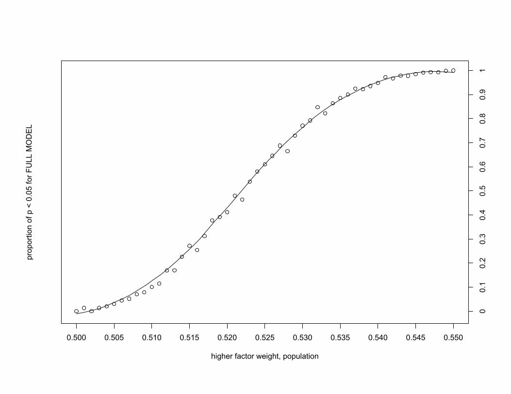
sociolinguis2cs sugges2ons (DEJ) • oken compare set of significant predictors, coefficients across groups, varie2es
• don’t compare coefficients from diff. models
• “significance” depends on many things – number of tokens – chance (distribu2on of speakers, words) – chance (plain chance)
• don’t force binary dis2nc2on, signif. vs. n.s. • best: compare models to test hypotheses
• publish complete data, allow re-‐analysis?

• thanks to: • Kyle Gorman • Sali Tagliamonte • workshop par2cipants
• please contact me: • danielezrajohnson @gmail.com
• these slides are at: • danielezrajohnson.com/ stepwise.pdf
Recommended