WinBUGS for population ecologists: Bayesian
modeling using Markov chain Monte Carlo
methods
Olivier Gimenez1, Simon Bonner
2, Ruth King
3, Richard A. Parker
3, Stephen P.
Brooks4, Lara E. Jamieson
4, Vladimir Grosbois
5, Byron J. T. Morgan
6, and Len
Thomas3.
1CEFE / CNRS; UMR 5175; 1919, Route de Mende; 34293 Montpellier Cedex 5; France
2Department of Statistics and Actuarial Science, Simon Fraser University, Burnaby BC, V5A 1S6
3Centre for Research into Ecological and Environmental Modelling, University of St Andrews, The
Observatory, St Andrews, KY16 9LZ
4The Statistical Laboratory – CMS, University of Cambridge, Wilberforce Road, Cambridge CB3 0WB,
U.K.
5Laboratoire Biométrie et Biologie Evolutive, UMR 5558, Bat. 711. Université Claude Bernard Lyon 1,
43 Boulevard du 11 novembre 1918, F-69622 Villeurbanne Cedex, France
6Institute of Mathematics, Statistics and Actuarial Science. University of Kent, Canterbury. Kent, CT2
7NF - ENGLAND

Abstract. The computer package WinBUGS is introduced. We first give a brief introduction to Bayesian
theory and its implementation using Markov chain Monte Carlo (MCMC) algorithms. We then present
three case studies showing how WinBUGS can be used when classical theory is difficult to implement.
The first example uses data on white storks from Baden Württemberg, Germany, to demonstrate the use
of mark-recapture models to estimate survival, and also how to cope with unexplained variance through
random effects. Recent advances in methodology and also the WinBUGS software allow us to introduce
(i) a flexible way of incorporating covariates using spline smoothing and (ii) a method to deal with
missing values in covariates. The second example shows how to estimate population density while
accounting for detectability, using distance sampling methods applied to a test dataset collected on a
known population of wooden stakes. Finally, the third case study involves the use of state-space models
of wildlife population dynamics to make inferences about density dependence in a North American duck
species. Reversible Jump MCMC is used to calculate the probability of various candidate models. For all
examples, data and WinBUGS code are provided.
Keywords: Bayesian statistics; density dependence; distance sampling; external covariates; hierarchical
modeling; line transect; mark-recapture; random effects; reversible jump MCMC; spline smoothing;
state-space model; survival estimation
Introduction
The Bayesian approach dates back to the Reverend Thomas Bayes and the 18th
century.
However, due to practical problems of implementing the Bayesian approach, little
advance was made for over two centuries. The development of new methodology
coupled with recent advances in computational power and the availability of flexible
and reliable software have led to a great increase in the application of Bayesian
methods within the last three decades, population ecology being no exception (Clark
2004; Ellison 2004; McCarthy 2007). Indeed, the application of the Bayesian theory in
population ecology has been greatly facilitated by the implementation of algorithms
known as Markov chain Monte Carlo (MCMC) methods (Gilks et al. 1996 and Link et
al. 1999 for an introduction for ecologists) in flexible and reliable software. For
example, MARK (White and Burnham 1999), one of the most popular computer
programs in population ecology, now includes an MCMC option which implements a
simple MCMC algorithm (White and Burnham this volume). AD Model Builder
(ADMB; Fournier 2001) is a general modeling environment for fitting complex models
to data, that has been used mainly in fisheries stock assessment (Maunder et al.
submitted), and has an MCMC option to implement Bayesian analysis (see Maunder et
al. this volume). Here we focus on the program WinBUGS (Bayesian inference Using
Gibbs Sampling; Spiegelhalter et al. 2003), which implements up-to-date and powerful
MCMC algorithms that are suited to a wide range of target distributions for analyzing
complex models.
The paper is organized as follows. We first review the Bayesian framework and show
how it can be fruitfully implemented using MCMC algorithms and program
WinBUGS. We then focus on three case studies to illustrate how WinBUGS can be
used to apply Bayesian methods using MCMC algorithms in population ecology. The
first example deals with mark-recapture models to estimate survival probabilities and
shows how to incorporate covariates with maximum flexibility. The second example
shows how to estimate population density while accounting for detectability by using
distance sampling methods. Finally, the third case study involves modeling count data
using state-space models. We conclude with a short discussion of various possible
extensions to both the methods and software that we have illustrated.
When presenting the examples, we include short illustrations in WinBUGS (code is
indicated using this typeface). For all three examples, the relevant data and full
WinBUGS code are given at http://eprints.st-andrews.ac.uk/archive/00000450/.
The Bayesian method using MCMC algorithms:
practical implementation in WinBUGS
Typical statistical problems involve estimating a vector of parameters, θ , using the
available data. The classical approach assumes that the parameters are fixed, but have
unknown values to be estimated. Classical maximum likelihood estimates generally
provide a point estimate of the parameter of interest. The Bayesian approach assumes
that the parameters themselves have some unknown distribution. The approach is
based upon the idea that the experimenter begins with some prior beliefs about the
system, and then updates these beliefs on the basis of observed data. Using Bayes’
Theorem, the posterior distribution of the parameters given the data ( )data|θπ has
density proportional to the product of the likelihood of the data given the parameters
( )θ|dataL and the prior distribution of the parameters ( )θπ :
( ) ( ) ( )θπθθπ ×∝ || dataLdata . The prior distribution represents the expert’s belief,
before observing any data. If there is no strong prior information on the parameters,
vague priors are typically specified on the parameters which represent very weak
opinion concerning the model parameters. Unfortunately, in most realistic applications
the posterior distribution is generally of such high dimension that little useful inference
can be obtained directly. As a consequence, while the joint posterior distribution (or
the corresponding marginal distributions) provide the best summaries of the
parameters, point estimates and uncertainty intervals are often more interpretable. It is
the process of summarizing the posterior that is the source of the computational
complexity of the Bayesian approach. Estimating the summary statistics of interest (for
a vector of parameters θ ) requires elimination of the other parameters. The Bayesian
approach does this through integration using the MCMC algorithm. The high-
dimensional integral associated with the posterior density is actually estimated using
appropriate Monte Carlo integration, which consists of constructing a Markov chain
with stationary distribution equal to the posterior distribution of interest. Then, once
the chain has converged, realizations can be regarded as a dependent sample from this

distribution. WinBUGS implements powerful ways of constructing these chains,
adapting to a wide range of target (posterior) distributions and therefore allowing a
large number of possible models to be fitted. Further details on Bayesian modeling
using MCMC algorithms can be found in Gilks et al. (1996) and Congdon (2003,
2006). The WinBUGS software is currently freely available at http://www.mrc-
bsu.cam.ac.uk/bugs/.
In outline, a typical WinBUGS session proceeds as follows:
The user specifies the model to run in the form of the likelihood and prior distributions
for all parameters to be estimated. Data and initial values must also be provided.
Following the validation of the user specification, MCMC simulations are generated
such that the stationary distribution of the Markov chain is the posterior distribution of
interest. Thus, this algorithm provides a sample from the posterior distribution of
interest from which, it is possible to produce estimates of the posterior distributions
using kernel density estimates, and summary statistics of interest such as posterior
medians and credible intervals. Convergence diagnostics are also available either
directly in WinBUGS or using the R packages CODA (Plummer et al. 2004) or BOA
(Smith 2004). Note that we will not discuss this crucial issue here, but
recommendations can be found in Kass et al. (1998). An important feature of
WinBUGS is that it comes with a tutorial designed to provide new users with a step-
by-step guide to running an analysis in WinBUGS. There are also a wide range of
varied and detailed examples, including, for instance: logistic regression with random
effects, analyses of variance with repeated measurements, meta-analyses and survival
analyses with frailties. It is often useful to call WinBUGS from other programs in order
to input complex sets of data and initial values, avoid specifying the parameters to be
monitored in each run, post-process the results in other software, display complex
graphics or perform Monte Carlo studies running WinBUGS iteratively in a loop.
Together with data and WinBUGS codes, we give an illustration of the use of the R
(Ihaka and Gentleman 1996; R Development Core Team 2007) package R2WinBUGS
(Sturtz et al. 2005), as well as an illustration of how to call WinBUGS from MATLAB
using the package MATBUGS
(http://www.cs.ubc.ca/~murphyk/Software/MATBUGS/matbugs.html) at
http://eprints.st-andrews.ac.uk/archive/00000450/. Other programs that can be used to
interface to WinBUGS are listed on the WinBUGS web page given above. General and
complementary introductions to WinBUGS are given in Congdon (2006) and
McCarthy (2007). We now turn to the analysis of real case studies to illustrate the use
of WinBUGS. Note that likelihoods and priors are implemented by defining their
probability distribution based on the model parameters using the tilde (~) symbol. This
notation will be used throughout the paper.
Estimating survival using mark-recapture data
As an illustration, we use data on the white stork Ciconia ciconia population in Baden
Württemberg (Germany), consisting of 321 capture histories of individuals ringed as
chicks between 1956 and 1971. From the 60’s to the 90’s, all Western European stork
populations were declining (Bairlein 1991). This trend is thought to be the result of
reduced food availability (Schaub et al. 2005) caused by severe droughts observed in
the wintering ground of storks in the Sahel region of Africa. This hypothesis has been
examined in several studies (Kanyamibwa et al. 1990, Barbraud et al. 1999; Grosbois
et al. in revision). In this section, we use WinBUGS and several of its features to
further explore the relationship between rainfall in the Sahel and survival probabilities
of the Baden Württemberg white stork population.
Simple models
The standard Cormack-Jolly-Seber model (CJS, Cormack 1964; Jolly 1965; Seber
1965; Lebreton et al. 1992) considers time-dependence for the probability iφ that an
individual survives to occasion 1+i given that it is alive at time i , and for the
probability jp that an individual is recaptured at time j . The data consist of encounter
histories for each individual made of 1’s corresponding to recapture or resighting and
0’s otherwise. These data can be efficiently condensed in the so-called reduced m-array
(e.g. Lebreton et al. 1992) which summarizes the data in the form of the number of
individuals released per occasion i, denoted Ri, and the number of first recaptures given
release at occasion i at the succeeding occasions j, denoted mij. The m-array for the
white stork data is provided in Tab. 1.
Table 1 around here

Conditioning on the numbers released and assuming independence among cohorts, the
CJS model likelihood can be written as a product of multinomial probability
distributions corresponding to each row of the m-array. The probabilities
corresponding to the m-array cells are complex nonlinear functions of the survival and
detection probabilities. For example, the probability of the number of individuals
released at occasion 3 and recaptured for the first time at occasion 5, given the number
of released individuals at occasion 3 is:
( ) 5443 1 pp φφ − . (1)
For further details of fitting the CJS model in a Bayesian framework, see Brooks et al.
(2000). We start with a simple mark-recapture model, a simplification of the CJS
model where, based on the conclusions of previous studies (Kanyamibwa et al. 1990;
Grosbois et al. in revision), the recapture probabilities are considered constant over
time.
Defining priors
We define priors for the survival probabilities and the recapture probability as Beta
distributions with parameters 1 and 1 (equivalently uniform distributions between 0
and 1). Within WinBUGS, this is specified as:
for (i in 1:ni) {phi[i] ~ dbeta(1,1)}
p ~ dbeta(1,1)
where ni is the number of occasions of release in the study.
Constructing the Likelihood
The likelihood is defined as a product of multinomial distributions using the function
dmulti:
for (i in 1:ni) {m[i,1:(nj+1)] ~ dmulti(q[i,],r[i])}
where the m object is the m-array matrix of data (augmented by the number of
individuals never seen again after release in the last column), nj is the number of
recapture occasions within the study, r is the vector of released individuals and q is a

matrix of the m-array cells probabilities. The q matrix and r vector are calculated in the
WinBUGS code.
Results
The posterior medians of the survival probabilities are displayed in Fig. 1a, along with
their posterior 95% credible intervals.
Figure 1 around here
To check that the temporal variations in the survival are worth considering, we also
consider a compromise approach in which survival is taken as constant over time.
Starting from the code of the previous model, one way to proceed would be to consider
one scalar parameter for the survival, specify the prior distribution as for the detection
probability and modify the likelihood accordingly. A neat trick which avoids
modifying the likelihood part of the code, is to define a single dummy variable with a
Beta prior and then set all survival probabilities equal to that variable:
# U(0,1) prior distribution for dummy variable
constant.phi ~ dbeta(1,1)
# All survival probabilities equal to dummy variable
for (i in 1:ni) {phi[i] <- constant.phi}.
DIC for Model Selection
As a preliminary model selection technique, we use the Deviance Information
Criterion (DIC; Spiegelhalter et al. 2002). One interpretation of the DIC is as a
Bayesian counterpart to the AIC for model selection. Essentially, the DIC is a
diagnostic that balances the requirements of model fit and low complexity. Typically,
as models get more complex by the addition of extra parameters, their fit improves.
The DIC diagnostic therefore penalizes additional parameters so that a parsimonious
model is chosen, and the smaller the DIC value, the better the compromise is. One
advantage is that the DIC can be calculated directly in WinBUGS from the chains
produced by an MCMC run. However, the DIC statistic is in its infancy and is
controversial (see the discussion papers following Spiegelhalter et al. 2002 and Celeux

et al. 2006). Here we consider the DIC as a preliminary tool for comparing competing
models, and we will discuss a more rigorous approach later, in the form of posterior
model probabilities.
Examining the DIC values in Tab. 2, we see that the time-dependent model appears to
outperform the constant model, and hence is better supported by the data. This suggests
that dependence upon time is needed to explain variations in the survival probabilities.
To better understand these findings, we will consider in the next section environmental
covariates as possibly explaining time variation in the survival probabilities.
Table 2 around here
Incorporating linear effects of covariates
We now turn to the incorporation of covariates in the CJS model (North and Morgan
1979; Pollock et al. 1984; Clobert and Lebreton 1985; Lebreton et al. 1992; see
Pollock 2002 for a review). As we mentioned earlier, the variation in white storks
survival is likely to be related to rainfall variations. As expected, it can be seen that the
variations in the survival estimates (Fig. 1a) are correlated to Sahel rainfall variations
(Fig. 1b). According to Williams et al. (2002: p.373), we therefore consider a model
including a linear effect of the rainfall covariate on the logit scale:
( ) i
i
i
i x211
loglogit ββφ
φφ +=
−= , (2)
where ix is the value of the covariate between occasions i and i+1, and the β ’s are
regression parameters to be estimated. We use normal distributions with mean 0 and
large variance (106) as vague prior distributions for those parameters. The rainfall
measurements are standardized to improve mixing within the Markov chain. Note that
the standardization can be implemented in WinBUGS:
for (i in 1:ni) {cov[i] <- (cov[i] - mean(cov[]))/sd(cov[])}
where cov[i] denotes the covariate value in year i.
The code provided in the previous section is amended as follows:
for (i in 1:ni) {logit(phi[i]) <- beta[1] + beta[2] * cov[i]}
for (j in 1:2) {beta[j] ~ dnorm(0,1.0E-6) �.
Note that in WinBUGS, normal distributions are described in terms of a mean and
precision, where precision = 1/variance. As a consequence, a variance of 1000000
corresponds to a precision of 0.000001. In addition, we note that this model makes the
strong assumption that variation in the survival probabilities is explained by the
covariate. This can be relaxed by the inclusion of additional random effects.
Incorporating random effects
We consider two models with random effects in this section, both addressing two
different questions. Note that incorporating random effects is also a way to share
information among parameters, particularly improving estimates for years where there
is little information in the data (e.g. Harley et al. 2004).
First, specifying constant survival probabilities can be too restrictive to capture sources
of temporal variability, while estimating as many parameters as time intervals may be
too costly to assess specific time trends (Burnham and White 2002; Royle and Link
2002). We consider a compromise model where time is treated as a random effect, ε ,
with a normal distribution with mean 0 and variance 2σ . We therefore estimate the
mean logit survival probability, say µ , and the temporal process variance in survival
probability 2σ (Gould and Nichols 1998, Burnham and White 2002):
( ) ii εµφ +=logit , (3)
Considering random effects raises the problem of calculating the likelihood, which is
obtained by integrating over the random effect ε . This is, indeed, a problem involving
a high-dimensional integral that could be handled by using approximations (Chavez-
Demoulin 1999), circumvented by resorting to asymptotic arguments (Gould and
Nichols 1998, Burnham and White 2002), or numerical integration (e.g. importance
sampling: Skaug and Fournier 2006 or Gaussian quadrature: Wintrebert et al. 2005).
By contrast, the Bayesian approach provides an exact solution to this problem (Brooks
et al., 2000; 2002; note that both references contain WinBUGS code) and WinBUGS
offers a powerful and flexible alternative to standard software such as MARK (White
and Burnham 1999) or M-SURGE (Choquet et al. 2005).
The specification of the model for the survival probabilities was as follows:
for (i in 1:ni) {

logit(phi[i]) <- logitphi[i]
logitphi[i] ~ dnorm(mu,taueps)
}.
We consider an inverse-gamma distribution with parameters 0.01 and 0.01 and a
normal distribution with mean 0 and large variance (100) as vague prior distributions
for taueps and respectively mu:
taueps ~ dgamma(0.01,0.01)
mu ~ dnorm(0,0.01).
Note that a gamma distribution for the precision is equivalent to an inverse-gamma
distribution for the variance. In this case, these are typical specifications of vague
priors (see also Lambert et al. 2005; van Dongen 2006; Gelman 2006). The posterior
distribution of the variance can easily be obtained by monitoring the quantity
sigma2eps defined as:
sigma2eps <- 1/taueps.
Second, the inclusion of random effects allows there to be additional variability within
the survival rates that can be attributed to natural variability, or temporal variability not
explained by the covariates within the study. This is a simple extension of the above
covariate model. In particular, we specify an additional random effect term denoted by
ε , which has a normal distribution with mean 0 and variance 2σ . In particular we
model the survival rate to be of the form:
( ) iii x εββφ ++= 21logit . (4)
Then, the parameters to be estimated are the regression coefficients ( β ’s) and the
random effect variance parameter 2σ . In a particular application, Barry et al. (2003)
noticed that omitting the random effect can lead to overestimation of the significance
of the covariate on survival. To include these additional random effects, the code is
modified as follows:
for (i in 1:ni){
logit(phi[i]) <- logitphi[i]
logitphi[i] ~ dnorm(f[i],taueps)
f[i] <- beta[1] + beta[2] * cov[i]
}
taueps ~ dgamma(0.01,0.01).
In our model, slope estimates produced using Eqns. 2 and 4 to model survival are very
close to each other: posterior medians for the slope 2β were 0.36 in both cases with
95% credible intervals [0.14; 0.58] and [0.20; 0.55] (see Fig. 2). This may indicate that
the random effect was not needed in the model, as the estimates tend to confirm (the
distribution of 2σ places all of its mass near 0 with posterior median 0.04 and 95%
credible interval [0.01; 0.22]), and indicated by the preliminary DIC analysis (see Tab.
2).
Figure 2 around here
A formal way of testing the null hypothesis 02 =σ will be discussed later. In both
cases, the effect of rainfall is positive, indicating that the more it rained in the Sahel
zone, the better storks survived.
Nonparametric modeling
There is another strong assumption made in Eqn. 2, namely that the effect of the
covariate on the survival probability is linear on the logit scale. However, nonlinear
relationships involving the impact of environmental factors on population dynamics
may occur (Mysterud et al. 2001). More flexible models for the survival probability are
therefore needed. Gimenez et al. (2006a; see also Gimenez and Barbraud this volume
and Gimenez et al. 2006b for a similar approach applied to individual covariates) have
recently proposed a method in which the shape of the relationship is determined by the
data without making any prior assumption regarding its form, by using penalized
splines (P-splines; Ruppert et al. 2003). Here, we give details of how to implement
their approach in WinBUGS. We consider the following regression model for the
survival probability iφ :
( ) ( ) iii xf εφ +=logit , (5)
where ix is the value of the covariate between occasions i and i+1, f is a smooth
function and iε are i.i.d. random effects ( )2,0 εσN . The function f specifies a
nonparametric flexible relationship between the survival probability and the covariate
that allows nonlinear environmental trends to be detected. Following Gimenez et al.
(2006a), we use a truncated polynomial basis to describe f :
( ) ( )∑=
+−++++=
K
k
P
kk
P
P xbxxxf1
10 κβββ K , (6)
where x is the covariate, and KP bb ,,,,,, 110 KK βββ are regression coefficients to be
estimated, 1≥P is the degree of the spline, ( ) ppuu =+ if 0≥u and 0 otherwise, and
Kκκκ <<< ...21 are fixed knots. We use
= 35,
4
1min IK knots to ensure the desired
flexibility, and let kk be the sample quantile of x 's corresponding to probability
1+K
k. Those quantities are calculated outside WinBUGS in program R. In particular,
we model the relationships using a linear ( 1=P ) P-spline with 4=K knots
implemented through the WinBUGS constants degree and nknots. To avoid overfitting,
we penalize the b ’s by assuming that the coefficients of ( )P
kx+
− κ are normally
distributed random variables with mean 0 and variance 2bσ to be estimated. This is the
reason why this approach is referred to as penalized splines (Ruppert et al. 2003). Note
that an alternative to P-splines called adaptive splines (Biller 2000) is considered in the
mark-recapture context by Bonner et al. (this volume). The penalization is achieved by
specifying:
for (k in 1:nknots) {b[k] ~ dnorm(0,taub)}
where the variance parameter is given an inverse-gamma distribution (i.e. the precision
has a gamma distribution):
taub ~ dgamma(0.001, 0.001).
A by-product of this approach is that the amount of smoothing is automatically
calculated as 22 / εσσ b . To implement the P-splines model in WinBUGS, it is convenient
to express it as a Generalized Linear Mixed Model (GLMM), as shown by Crainiceanu
et al. (2005). If X is the matrix with ith row ( )TP
iii xxX ,,,1 K= and Z the matrix with

the ith row ( ) ( )( )TP
Ki
P
ii xxZ++
−−= κκ ,,1 K , then an equivalent model representation of
Eqns. 5 and 6 in the form of a GLMM is given by Gimenez et al. (2006a):
( ) εβφ ++= ZbXlogit ,
=
I
Ibb
2
2
0
0cov
εσ
σ
ε (7)
We are now able to implement the P-splines model in WinBUGS. To code Eqn. 7, we
used:
for (i in 1:n){
logit(phi[i]) <- logitphi[i]
logitphi[i] ~ dnorm(f[i],taueps)
f[i] <- inprod(beta[],X[i,]) + inprod(b[],Z[i,])
}.
The first statement corresponds exactly to Eqn. 6, the second implements the random
effects distribution and the last one specifies the structure of the mean logit survival,
where the function inprod denotes the inner product of two vectors. The first part of the
last statement contains the fixed effect of Eqn. 7, where beta[] is the vector
( )210 ,, ββββ = , X[i,] is iX and inprod(beta[],X[i,]) is the polynomial part. The second
part of the last statement contains the random effects, where b[] is the vector
( )4321 ,,, bbbbb = , Z[i,] is iZ and inprod(b[],Z[i,]) is the truncated polynomial part of the
regression in Eqn. 7.
We then obtain matrices X and Z directly in WinBUGS, although this step could be
done in program R for example. Matrix X is obtained as:
for(i in 1:n) {
for(l in 1:degree+1) {
X[i,l] <- pow(covariate[i],l-1)
}
}
where pow is the power function, and pow(a,b) is ba . Matrix Z is obtained using:
for (i in 1:n){
for (k in 1:nknots){
Z[i,k] <- pow((covariate[i]-knot[k]) *
step(covariate[i]-knot[k]),degree)
}
}
where the function step is used to obtain the truncation, where step(x) is 1 if x is
positive and 0 otherwise, so that Z[i,k] is positive only for kix κ> . For further details
see Crainiceanu et al. (2005) and Gimenez et al. (2006a). With the possibility of fitting
nonparametric models, one is obviously interested in testing for the presence of
nonlinearities in the survival probability regression. We address this question by using
the DIC and also using visual comparison for comparing the model with a linear effect
of rainfall as well as a random effect (see previous section) to its nonparametric
counterpart. Fig. 3 shows that the relationship between rainfall in Sahel and white stork
survival can be taken as linear. This is confirmed by DIC values that are similar for
these two models (Tab. 2). Although we have clues for linearity in this example, the
issue of formally detecting nonlinearity deserves further investigation.
Figure 3 around here
Dealing with missing data
Bayesian modeling via MCMC also provides a simple method for handling data with
missing covariate values. Missing data might occur in capture-recapture studies if the
value of an environmental covariate is not recorded on all occasions or if an individual
covariate changes over time and can only be observed on the occasions when the
specific animal is captured (Bonner and Schwarz 2006). Essentially, a completed data
set is generated on each iteration of the MCMC algorithm by specifying an underlying
model for the covariate and imputing the missing values of the covariate using the
current values of the parameters, and then the completed data set is used to update the
parameter values. The result is a sample from the joint posterior distribution of both the
parameters and the missing data values, which can be used in Bayesian inference. We

illustrate the issue of dealing with missing data by estimating the effect of rainfall in
the Sahel on the survival of the white storks in Baden Württemberg after deleting the
covariate for several years.
As with the model incorporating random effects, computing the value of the likelihood
for a given set of parameter values requires integration with respect to the missing
covariates. This can be a complicated numerical problem, especially if several values
are missing, and is an obstruction to computing maximum likelihood estimates and
their standard errors. From a Bayesian perspective, we view the missing covariates as
random variables to which we can assign a probability distribution, just like the model
parameters. We define a prior distribution for the missing covariate values and then
compute the posterior distribution of both the parameters and the missing values
conditional on the observed data. The likelihood function used in the analysis is
exactly the same function used when all covariate values are observed, and if MCMC
is used to obtain a sample from the posterior distribution then no additional integration
is required. Instead, a sample of probable values for the missing covariates is generated
by sampling new values on each iteration of the MCMC algorithm in exactly the same
way that model parameters are sampled. The prior distribution of the missing covariate
can be chosen to capture prior beliefs about the values of the missing covariates and
their relation to the rest of the data. A simple, vague prior for the rainfall in year i, ix , is
the normal distribution with mean 0 and large variance ( )610,0~ Nxi . This prior
distributes its mass evenly over a very wide range of values and assumes independence
of the rainfall across the years of the study. Alternative prior distributions will relate
the values of the covariates to each other or to other quantities. Here we use a
hierarchical prior that models the change in the covariate over time as
( )2
1 ,~ xii xNx σµ+− . This asserts that the change in the covariate between adjacent
years is normally distributed with the same mean and variance for all years.
Information from the observed covariate values will then be used in determining the
posterior mean and variance of the missing values. To complete the prior distribution
we must also specify the marginal distribution of the first covariate value, 1x , and the
distributions for the hyperparameters, µ and 2
xσ . Here we use the vague
prior )10,0(~ 6
1 Nx for marginal prior of the first covariate, and the standard vague
priors for a normal mean and variance: )10,0(~ 6Nµ and ( )01.0,01.0~ 12 −Γxσ .
Alternate prior specifications for the covariate values include autoregressive models,
regression of the covariate against time, or relation of the covariate to other variables
that might have been recorded. Adapting the WinBUGS code to account for the
missing covariate values requires two simple changes: (i) adding the prior distribution
for the covariates, and (ii) modifying the input data. The WinBUGS code for the
hierarchical prior is:
mu ~ dnorm(0,1.0E-6)
taucov ~ dgamma(.01,.01)
sigma2cov <- 1/taucov
cov[1] ~ dnorm(0,1.0E-6)
for(i in 1:(ni-1)){
mucov[i] <- cov[i] + mu
cov[i+1] ~ dnorm(mucov[i],taucov)
}.
The first three lines of code define the hyperpriors for the hyperparameters ( µ is mu
and 2
xσ is sigma2cov). The 4th
lines defines the marginal prior for 1x and the for loop
defines the distribution of each of the remaining covariate values conditional on the
previous value ( ix is cov[i]). Missing values in the input data are specified by replacing
the observed value with 'NA'. Suppose that the rainfall is observed in all years except
year 15; the input vector for the covariate is:
cov=c(.79,2.04,1.04,-.15,-.01,-.48,1.72,-.83,-.02,.14,-.71,.50,-.62,-.88,NA,-1.52)
Given this data and the model above, WinBUGS will simulate values for the
hyperparameters and the missing rainfall observation for year 15 on each MCMC
iteration and produce posterior summaries for these quantities, exactly as it does for the
other model parameters. Posterior summary statistics for a single run are shown in Tab.
3.
Table 3 around here

Estimates of the survival probabilities are almost exactly identical to the estimates
produced from the full data; differences in the posterior means and standard deviations
are the magnitude as the MCMC error. There is a very slight increase in the posterior
variability of the regression coefficients, 1β and 2β , however the lower bound of the
95% credible interval for 2β is still well above 0 indicating a clear positive link
between rainfall and the storks’ survival. The estimated mean change in rainfall is -.15
with 95% credible interval (-.85,.56) which suggests that there is no consistent trend
over time. The standard deviation of the change in rainfall is relatively large which
indicates that there is little association between rainfall in adjacent years. Because of
this, the posterior distribution for rainfall in the missing year is uninformative about the
true value.
When 5 missing values are generated, there are only minor differences in the posterior
distribution of the survival probabilities with small increases in the standard deviation
apparent for the years with the covariate deleted (Tab. 3). This is not surprising
because the capture probabilities are very high so that most information about the
survival probabilities is derived from a direct comparison of the capture histories rather
than the regression on the covariate. There is, however, significant change in the
inference for the regression coefficients. The posterior mean of the slope, 2β , is closer
to 0 in Tab. 3, though whether the mean is increased or deceased depends on which
years are missing the covariate. More importantly, the posterior standard deviation is
increased from 0.11 to 0.13 and the 95% credible interval contains 0 which brings the
effect of rainfall on survival into doubt.
To close this section, we note that we have only considered rainfall at a single
meteorological station in the Sahel region. However, rainfall measurements at other
stations are available, therefore possibly providing a better spatial representation of the
white storks’ wintering area. The question is then to determine which combination of
the stations best explains the variation in survival. If we have 10 stations, we need to
perform model selection among a set of 1024 (210
) possible candidates, which would
be intractable using classical model selection criteria such as AIC, BIC or DIC.
Fortunately, an alternative method can be used that allows model selection among a
large set of candidate models. An example is given later in the section dealing with
state-space modeling of count data, and we have made available the WinBUGS code to
implement this approach on the stork dataset.
Estimating abundance and population density using
line-transect data
Line transect surveys are widely used to estimate the density and/or abundance of
wildlife populations. The methods, which are a special case of a general approach
called distance sampling, are described in detail, from a classical perspective, by
Buckland et al. (2001, 2004a). Observers walk along a set of randomly located transect
lines recording the perpendicular distance to all detected objects of interest (usually
animals) within some detected with some perpendicular truncation distance w. Not all
objects within distance w are assumed to be detected; rather a (semi-) parametric model
is specified for the probability of detecting an object given it is at perpendicular
distance y from the transect line. Under various assumptions (detailed in Buckland et
al. 2001), it is then possible to derive the probability density function f(y) of observed
distances. This can be fitted to the observed distance data using maximum likelihood
methods, and used to correct for the objects missed during the survey. The standard
formula for estimating object density, D, is (Buckland et al. 2001):
( )L
fnD
2
0ˆˆ = (8)
where n is the number of objects detected, L is the total length of the transect lines and
( )0f̂ is the estimated probability density function of observed distances evaluated at
zero distance.
As an illustration, we consider a line transect study where a known number of wooden
stakes are placed in a sagebrush meadow east of Logan, Utah (Buckland et al. 2001).
The true density of stakes is known to be 37.5 stakes/hectare. Eleven different graduate
students walked a 1,000 m long transect through the study area independently of one
another and recorded perpendicular sighting distances to stakes. One student’s data are
given in Tab. 4.
Table 4 around here

These data consist of 68 observations with a truncation width, w, of 20 m. The same
data set is analyzed by Karunamuni and Quinn (1995) who propose a Bayesian
approach for line transect sampling. For the sake of simplicity, we make the same
assumptions as Karunamuni and Quinn (1995), i.e. we assume that the probability
density function f(y) for the detection distances is half-normal and that the data are
neither truncated nor grouped into distance intervals (see Buckland et al. 2001 for more
on the latter). Thus,
( ) ( ) ( ) 0,2/exp2/exp/2 2222 >−=−= yycyyf λλσπσ (9)
where π/2=c and 2/1 σλ = . Given n detection values, nyy K,1 , the maximum
likelihood estimator of ( )0f is then given by:
( )2
1
2
20ˆ
−
==
∑ n
Tc
y
nf
iπ (10)
where ∑= 2
iyT . The maximum likelihood estimator of the density is given by Eqn. 8,
above.
Adopting a Gamma prior distribution with parameters a and b for λ , Karunamuni and
Quinn (1995) show that the posterior distribution of λ is also a Gamma distribution
with parameters 2
na + and
1
2
1−
+
T
n. Although classical Monte Carlo simulations
could be used to simulate observations from the posterior distribution of λ , we use
WinBUGS to draw random samples using MCMC techniques. This is motivated by
generalizations to other probability density functions for the detection distances as well
as spatial modeling for which explicit posterior distributions are difficult to obtain. We
use the so-called “zeros trick” to implement the half-normal likelihood distribution L
because it is not included in the list of standard WinBUGS sampling distributions. This
method consists of considering an observed data set made of 0’s distributed as a
Poisson distribution with parameter φ so that the associated likelihood is ( )φ−exp .
Now, if we set phi[i] to ( )( )iLlog− where the likelihood term ( )iL is the contribution of
observed perpendicular distance y[i], then the likelihood distribution is clearly found to
be ( )iL . See the WinBUGS manual for further details. The WinBUGS code is as
follows:

for (i in 1:n) {
zeros[i] <- 0
zeros[i] ~ dpois(phi[i]) # likelihood is exp(-phi[i])
# -log(likelihood)
phi[i] <- - (log(2*lambda/3.14)/2 - lambda * pow(y[i],2) / 2)
}.
Karunamuni and Quinn (1995) conduct a sensitivity analysis showing that changing
values of the prior distribution has little effect on the posterior results. To allow
comparisons with Karunamuni and Quinn’s results, we use a = b = 0.1 in our analyses.
For parameter λ , we therefore specify a gamma distribution with both parameters set
equal to 0.1:
lambda ~ dgamma(0.1, 0.1).
Finally, we calculate an estimate of )0(f and the density D (Eqns. 8 and 10):
f0 <- sqrt(2 * lambda / 3.14)
D <- (n * f0)/(2 * L).
The results are given in Tab. 5 and show close agreement with the Bayesian analysis of
Karunamuni and Quinn (1995).
Table 5 around here
State-space models of count data: assessing density
dependence
In this section, we describe the use of WinBUGS to fit population models of density
dependence that simultaneously account for both process and observation error. The
example data we use are annual estimates of the population size of North American
duck species on their breeding grounds from 1955 to 2002, derived from the
Waterfowl Breeding Population and Habitat Survey (WBPHS, US Fish and Wildlife
Service 2003).
Assessing the importance of population size or density in regulating population growth
rate is fundamental to population biology, ecology and conservation. However,
devising robust tests for this so-called “density dependence” has been controversial
(e.g. Lebreton this volume). One problem has been that available data on population
sizes or densities are almost always estimates, with some level of observation error,
and ignoring this observation error can lead to biased tests (e.g. Shenk et al. 1998).
A potential solution is to use a state-space modeling framework, where one can
explicitly specify models for both the underlying population dynamics that change
population size over time and the observation process that links true population size to
the estimates. Such models describing density dependence were constructed by
Jamieson (2004) and Jamieson and Brooks (2004). Here we take as an example their
“logistic” model for the population dynamics (“state process model”), which can be
written as follows:
++= ∑
=
−− tpp
k
j
jtjtt znnn ,
1
01 exp σββ (11)
where nt is the population size at time t (t = 1…,T), β0 determines the expected rate of
population growth when the population size is zero, β j determines the rate at which
growth is changed depending on population size in time period t-j, zp,t is a Gaussian
N(0,1) random variable that represents un-modeled variation in population growth
between time periods (“process error”) and σ p determines the size of these random
fluctuations. This is coupled with an “observation process model”, which can be
written
totott zsny ,,+= (12)
where yt is the estimated population size at time t, zo,t is a Gaussian N(0,1) random
variable that represents measurement error and so,t, which is assumed known (it is
provided as part of the WBPHS data, for example), determines the size of the
measurement errors.
The state-space model defined by Eqns 11 and 12 is non-linear and non-normal
(because of Eqn. 11), and therefore is tricky to fit using standard frequentist methods,
such as the Kalman filter (although see de Valpine 2002, 2003, de Valpine and
Hastings 2002, Besbeas et al. 2005, Besbeas et al. this volume). Jamieson (2004) and

Jamieson and Brooks (2004) describe how the model can be formulated in a Bayesian
context, and how the parameters may be estimated, for fixed k, using MCMC.
Further, they show how a recent extension of the MCMC algorithm – Reversible Jump
MCMC (RJMCMC; Green 1995) – can be used to compute the posterior probability
for each of a set of possible values of k, and thereby estimate the probability of the
presence of density dependence (i.e., the probability that k>0) in a population
(although we note that autocorrelated process error can affect such assessments – see
Lebreton this volume). For the use of RJMCMC in population ecology, see for
example, King and Brooks (2002a, b; 2003; 2007) and King et al. (submitted).
RJMCMC can also be used to produce model-averaged predictions of future
population size. Jamieson and Brooks (2004) apply these methods using custom-
written MCMC and RJMCMC samplers, implemented in the computer language C, to
data for 10 species of duck from the WBPHS. Three species (Northern Pintail Anas
acuta, Redhead Aythya americana and Canvasback Aythya valisineria) appear to show
some form of density dependence.
Similar models were fitted to Canvasback and Mallard data from the WBPHS (as well
as simulated data) by Viljugrein et al. (2005) using WinBUGS, although code was not
included with that paper. An additional covariate, number of breeding ponds, was
included and model discrimination was via DIC. In this paper, both species were found
to show density dependence.
Our aim is to demonstrate how these models may be fitted using WinBUGS, to
investigate the use of the beta version of the RJMCMC plug-in for WinBUGS, and to
validate the results by comparing them with the independent sampler and C code
written by Jamieson. We present some of this work here; it is described in detail in
Parker et al. (in prep). To save space, we only present results for Canvasback.
Logistic model
For computational convenience, we re-parameterized the model presented above so
that time periods kt ,,1K= are the times before data are available and
Tkkt ++= ,,1K are times when data were collected. Note that missing data are easily
accommodated in this framework. We also turned Eqn. 11 into an additive model by
log-transforming:
( )tp
k
j
jnjtt zppp σββ +++= ∑=
−−1
01 exp (13)
where pt = log(nt).
Bayesian methods require specification of prior distributions on all unknown
quantities; for the purposes of comparison we used exactly the same distribution as
used in Chapter 2 of Jamieson (2004; note these are slightly different from those of
Jamieson and Brooks 2004): )100,0(~ Njβ for kj ,,0 K= ,
)001.0,001.0(12 −Γ=pσ
and )130.0,540.0(~ Nnt for kt ,,1K= . Note that numbers of ducks are expressed
x106 and that the distribution is truncated so that
0>tn (by setting all sampled values
of nt to the maximum of the value drawn from the above normal distribution and
0.00001). Priors are not required on tn, Tkkt ++= ,,1K due to the Markovian
structure of the state process model: priors for these quantities are implicitly specified
when priors are set for tn, kt ,,1K= . (See Jamieson 2004 for an in-depth discussion
of this; see also de Valpine 2002 and Maunder et al. this volume).
Our WinBUGS program was based on code originally written by Steve Brooks for a
workshop on Bayesian methods (Brooks et al. 2005). The key parts are specification of
the observation process equation (Eqn. 12) and system process equation (Eqn. 13).
The observation process equation code is:
for (t in (k+1):T){
prec[t] <- 1/(s[t]*s[t])
m[t] ~ dnorm(n[t],prec[t])
}
while the system process equation code is:
for (t in (k+1):T){
#mm is used to build up equation 3 - note that b[1] here is
#beta_0 in equation 1, b[2] is beta_1, etc.
mm[1,t] <- p[t-1] + b[1]
for (j in 1:k){ mm[j+1,t] <- mm[j,t] + b[j+1]*exp(p[t-j]) }
# Expected value of p[t]

Ep[t] <- mm[k+1,t]
# Realized value, with process error - tau is 1/sig_p^2
p[t] ~ dnorm(Ep[t],tau)
}.
Predictions of future states, for example up to time 10+T , could easily be obtained by
replacing the first line of the above loop with
for (t in (k+1):(T+10)){.
Summaries of the posterior parameter estimates for Canvasback for ,2,1=k and 5 and
runs with burn-in of 50,000 and then 1,000,000 samples are given in Tab. 6, as are
results from the same model reproduced from Jamieson (2004, Table 2.5).
Table 6 around here
The results are very similar, with differences within the bounds of Monte-Carlo
variation. Convergence and mixing were relatively slow; diagnostics are reported in
Parker et al. (in prep.).
A naïve way to look for evidence of density dependence is to examine posterior
credibility intervals (CI) on the β parameters. For example, in the first-order time lag
model ( 1=k ), the 95% posterior CI does not contain 0 throughout, providing support
for the notion of first order density dependence in this species.
Model comparison
The above program was extended to allow selection among models using RJMCMC.
This algorithm searches over the different models, given the observed data, so that the
number of possible models is no longer restrictive. We consider an extension to the
standard Bayes Theorem, where we simply consider the model itself to be a (discrete)
parameter. The standard formula still applies, but now the posterior distribution is
defined over both the parameter and model space. Integrating over the parameters we
are able to calculate the marginalized posterior probability for each model. However,
this integration is analytically intractable and so we resort to an MCMC-type approach.
The standard MCMC algorithm cannot be used in the presence of model uncertainty,

and RJMCMC are therefore used to explore simultaneously the parameter and model
space within a single Markov chain. We used the Jump extension to WinBUGS (Lunn
et al., 2006) to implement RJMCMC. This extension allows the sampler to move
between models that include all possible combinations of a set of potential covariates –
in our case β1 to βV where V is the maximum time lag allowable (set to 5 in our code). k
indexes the number of β parameters (excluding β0, which is in all models) in the model
for a particular draw from the chain (i.e., the dimension of the model). In the code, an
indicator variable id, indicates which particular model is in a particular draw – for
example if id was 10101, that would indicate that the parameters β1, β3 , and β5 were in
the model for that draw (and therefore that k = 3).
In the Jump protocol one specifies a prior on the models by specifying a prior
distribution on k. The following gives a prior probability of 0.5 that any βj ( Vj ≥>0 )
is in the model (Lunn 2006, p. 3):
k ~ dbin(0.5,V).
We then specify a design matrix (see Lunn 2006, Eqn. 1) with the number of rows
equal to the number of time periods and V columns. The elements of each row
correspond to the sum in Eqn. 13. In the following code, C is the first time period
about which we make posterior inferences in states – i.e., C=V+1.
for (t in C:T){
for (j in 1:V){
X[(t-C+1),j] <- exp(p[t-j])
}
}.
To set up the reversible jump, we use the two Jump-specific commands jump.lin.pred
and jump.model.id, as follows:
# Jump process
psi[1:(T-C+1)]<- jump.lin.pred(X[1:(T-C+1),1:V], k ,taub)
id <- jump.model.id(psi[1:(T-C+1)])

where psi is a vector representing the current values of the linear predictor (Lunn 2006,
Eqn. 1), and taub is the prior precision on the β parameters (in our case 1/100; note that
the prior on all beta parameters is assumed to be multivariate normal, with mean 0 and
the specified precision – this distribution is fixed by the software).
We note that the priors specified on the parameters can influence the corresponding
posterior model probabilities. In other words the posterior model probabilities are often
sensitive to the prior parameter specification. Thus we recommend that a prior
sensitivity analysis should always be performed, and care taken when specifying the
priors for the parameters, to represent sensible prior beliefs.
Lastly, we specify the system process equation in terms of the psi variable:
for (t in C:T){
# Expected value of p[t]
Ep[t]<-p[t-1]+psi[(t-C+1)]
# Realized value, with process error - tau is 1/sig_p^2
p[t] ~ dnorm(Ep[t],tau)
}.
Posterior model probabilities can be calculated from the proportion of time the chain
visited each model of interest. This information can be obtained from the Jump menu
that is added to the WinBUGS interface when the Jump extension is installed, and
reports the proportion of time spent in each value of the id variable. Note, however,
some of the models included in the chain are not of interest – we are only interested in
models that for any given k contain parameters β1,…, βk: for example with k = 2 we are
only interested in id 11000, and not 10100, 01100, etc. We therefore select out from the
list of id’s only those we are interested in, and re-normalize so that the proportion of
times in these models of interest sum to 1. These proportions are then estimates of
posterior model probability.
Model-averaged estimates of other unknown quantities, such as the nts, can also be
produced by WinBUGS, but just as with the ids above, these contain both models we
are interested in and those we are not. It is necessary to save the value for the variable
of interest generated in each sample (the CODA button in the sample monitor tool will

do this), as well as the corresponding id values, and then select out only those samples
that were generated under id values corresponding to models of interest.
Posterior model probabilities for Canvasback for runs with burn-in of 50,000 and then
1,000,000 samples are given in Tab. 7, as are results from the equivalent model from a
run of the Jamieson C code using burn-in of 20,000 and 100,000 samples (a run of the
Jamieson code was required because posterior model probabilities were not given for
these priors in Jamieson 2005).
Table 7 around here
While the results are similar, they are not identical. This is likely to be caused by a
small difference between the implementations: in the algorithm of Jamieson, the
acceptance probabilities for between-model moves do not depend on the priors for the
β parameters (Jamieson 2005: Section 3.1.1), while in the WinBUGS algorithm it is
not possible to achieve such tuning, and in the default algorithm the priors on the β
parameters do affect acceptance rates. Despite these minor differences, the overall
conclusions are the same: the best supported model (posterior model probability 0.6-
0.7) is the one with first-order density dependence.
Discussion
In this paper, we have seen how Bayesian theory can be applied to stochastic models
for population ecology using MCMC algorithms as implemented in program
WinBUGS.
In a mark-recapture data modeling context, WinBUGS can handle many complex
models, without additional effort once the likelihood has been written down. This
includes (i) random effects that allow unexplained residual variance to be coped with
when dealing with covariates, automatic calculation of the amount of smoothing when
splines are to be used but also temporal autocorrelation to be incorporated (Johnson
and Hoeting 2003), (ii) missing data in the covariate values to be handled and (iii)
variable selection. Note that those advantages may also be applied in distance sampling
models in order to incorporate covariates in the modeling of the detection function
(Marques and Buckland 2005; Marques et al. 2007). Random effects can also be used

to address spatial variation in both families of models, allowing the survival and the
detection function to depend on spatial coordinates (e.g. longitude and latitude) using
splines in two dimensions (Gimenez and Barbraud this volume) or a combination of
various random effects (Grosbois et al. in revision) or alternatively, using the
geostatistical tools as available through the GeoBUGS adds-on of WinBUGS and the
possibility of interfacing WinBUGS with Geographic Information System (GIS)
software (WinBUGS manual; see Wyatt 2003 for an application in fisheries).
In our experience, using R or MATLAB to call WinBUGS makes its use much easier
for pre- and post-processing data. Note also that an open-source version of the
WinBUGS code has recently been published as OpenBUGS. Among other advances, it
can be made to perform block updates (i.e., update multiple unknown quantities
simultaneously), which might be of interest for experienced programmers. OpenBUGS
also runs under Linux.
Our introduction may make WinBUGS appear like a panacea. However, like all
computer programs, WinBUGS is not always the perfect tool for Bayesian methods in
population ecology, and developments are taking place to improve it. However, as can
be appreciated from the three case-studies, it is capable of producing informative
results for sophisticated models. In using WinBUGS, one should be aware of the
following potential problems. First, one should be aware that experience is needed to
be able to debug WinBUGS programs. Also, the computational burden may be
discouraging, and it is sometimes preferable to resort to Fortran or C++ to implement
efficient MCMC algorithms for specific problems. Finally, although user-specific
functions can be programmed (see the WinBUGS manual), there are no tools for
matrix calculus so that, e.g., multistate mark-recapture models are difficult to
implement (see however Durban et al. 2005 for closed populations). Interestingly, a
state-space modeling approach for data on marked animals proposed by Gimenez et al.
(2007) might be a solution to this problem (see also Royle [in press] for a similar state-
space formulation allowing modeling individual effects). More generally, in line with
Buckland et al. (2004b; see also Newman et al. 2006; Buckland et al. 2007), we believe
that state-space modeling can provide a convenient and flexible framework for
specifying many stochastic models for the dynamics of wild animal populations. In
doing so, WinBUGS may provide an efficient and flexible tool to fit such models,
possibly nonlinear and non Gaussian – as has been realized for several years in
fisheries (Meyer and Millar 1999; Millar and Meyer 2000; Rivot and Prévost 2002;
Lewy and Nielsen 2003; Rivot et al. 2004). We note that other fitting algorithms, such
as variations on the Kalman filter, Monte-Carlo particle filter, Laplace approximation,
importance sampling may also be applicable (see Buckland et al. 2007 for a review).
These ideas open the area to numerous applications including the integration of several
sources of information (recovery and recapture data, see Catchpole et al. 1998; count
data and demographic data, see Besbeas et al. 2002, 2005; this volume; Brooks et al.
2004; Maunder 2004; Schaub et al. 2007).
We end by providing a non-comprehensive list of applications of Bayesian methods in
population ecology. An important advantage of the Bayesian framework is the
possibility to incorporate prior information in the analysis. McCarthy and Masters
(2005) show how to use prior information on body mass to improve survival estimates
using the CJS models, while Pearce et al. (2001), Yamada et al. (2003), Kuhnert et al.
(2005) and Martin et al. (2005) show how to integrate expert knowledge. Several
authors have dealt with important issues regarding the specification of vague priors
(Lambert et al. 2005; van Dongen 2006; Gelman 2006), assessment of the sensitivity of
the posterior distribution to the specified prior distribution (Millar 2004; Millar and
Stewart 2005), parameter identifiability in a Bayesian context (Gimenez et al. this
volume) and goodness-of-fit tests (Brooks et al. 2000; Barry et al. 2003; Michielsens
and McAllister 2004). Meta-analyses have been successfully carried out to estimate
demographic parameters (Tufto et al. 2000) and assess animal movement (Jonsen et al.
2003). Further applications of WinBUGS to analyze animal movement data can be
found in Morales et al. (2004) and Jonsen et al. (2005). WinBUGS can be used to
address issues associated with binomial and Poisson data such as spatial
autocorrelation (Thogmartin et al. 2005; Wintle and Bardos 2006), imperfect detection
(Royle and Dorazio 2006), heterogeneity in the detection process (Durban and Elston
2005), excess of zeros (Martin et al. 2005; Ghosh et al. 2006), observer effects
(Thogmartin et al. 2005), detecting trends (Link and Sauer 2002) and missing data
(Lens et al. 2002). WinBUGS has allowed a better understanding of the impact in
assessing complex effects of density-dependence and predicting the impact of climate
change and human exploitation in population dynamics (Bjornstad et al. 1999; Saether
et al. 2000; Stenseth et al. 2003; Conroy et al. 2005). Regarding model selection,
alternatives to DIC and RJMCMC using WinBUGS are given by Ntzoufras (2002;
Gibbs variable selection), Link and Barker (2007; Bayesian information criterion; see
also Link and Barker this volume) and Ghosh and Norris (2005; minimum posterior
predictive loss). Finally, Link et al. (2005) considered association among demographic
parameters (e.g. recruitment and survival) in analysis of open population mark-
recapture data (see also Cam et al. 2002 and Wintrebert et al. 2005 when detectability
is equal to one).
In conclusion, we hope this paper will encourage ecologists to explore the potential of
the flexible and useful WinBUGS software, and the methods underlying it, for carrying
out future applications.
References
Bairlein, F. (1991). Population studies of white storks ciconia ciconia in Europe, with
reference to the western population. In C. Perrins, J.-D. Lebreton and G. Hirons
(editors), Bird Population Studies: Relevance to Conservation and Management,
pages 207-229. Oxford University Press. Oxford.
Barbraud, C., J. C. Barbraud and M. Barbraud (1999). Population dynamics of the
White Stork Ciconia ciconia in western France. Ibis, 141: 469-479.
Barry, S. C., S. P. Brooks, E. A. Catchpole and B.J.T. Morgan (2003). The analysis of
ring-recovery data using random effects. Biometrics, 58: 54-65.
Besbeas, P., S. N. Freeman, B. J. T. Morgan and E.A. Catchpole (2002). Integrating
mark-recapture-recovery and census data to estimate animal abundance and
demographic parameters. Biometrics, 58: 540-547.
Besbeas, P., S.N. Freeman and B.J.T. Morgan (2005). The potential of integrated
population modelling. Austr. New Zeal. J. Stat., 47: 35-48.
Biller, C. (2000). Adaptive Bayesian Regression Splines in Semiparametric
Generalized Linear Models. Journal of Computational and Graphical Statistics, 9:
122-140.
Bjornstad, O. N., J. M. Fromentin, N. C. Stenseth and J. Gjosaeter (1999). Cycles and
trends in cod populations. Proceedings of the National Academy of Sciences of the
USA, 96: 5066-5071.
Bonner, S. J. and C. J. Schwarz (2006). An extension of the Cormack-Jolly-Seber
model for continuous covariates with applications to Microtus pennsylvanicus.
Biometrics, 62:142-149.

Brooks, S. P., E. A. Catchpole and B. J. T. Morgan (2000). Bayesian animal survival
estimation. Statistical Science 15, 357–376.
Brooks, S. P., E. A. Catchpole, B. J. T. Morgan and M. P. Harris (2002). Bayesian
methods for analysing ringing data. Journal of Applied Statistics, 29 :187-206.
Brooks, S.P., R. King and B. J. T. Morgan, (2004). A Bayesian approach to combining
animal abundance and demographic data. Animal Biodiversity and Conservation,
27: 515-529.
Brooks, S.P., Gimenez, O. and King, R. (2005) Bayesian Methods for Population
Ecology - Workshop Codes. National Centre for Statistical Ecology Software
Library. [http://www.ncse.org.uk/software.html].
Buckland, S. T., D. R. Anderson, K. P. Burnham, J. L. Laake, D. L. Borchers, and L.
Thomas. 2001. Introduction to Distance Sampling. Oxford University Press,
Oxford.
Buckland, S. T., D. R. Anderson, K. P. Burnham, J. L. Laake, D. L. Borchers, and L.
Thomas. Eds. 2004a. Advanced Distance Sampling. Oxford University Press,
Oxford.
Buckland, S.T., Newman, K.B., Thomas, L., Koesters, N.B., 2004b. State-space
models for the dynamics of wild animal populations. Ecological Modelling. 171,
157-175.
Buckland, S. T., K. B. Newman, C. Fernández, L. Thomas and J. Harwood (2007).
Embedding population dynamics models in inference. Statistical Science. 22, 44-
58.
Burnham, K. P., D. R. Anderson and J. L. Laake (1980). Estimation of density from
line transect sampling of biological populations. Wildl. Monogr., 72: 1-202.
Burnham, K. P. and G. C. White (2002). Evaluation of some random effects
methodology applicable to bird ringing data. Journal of Applied Statistics, 29: 245-
264.
Cam, E., W. A. Link, E. G. Cooch, J. Y. Monnat and E. Danchin (2002). Individual
covariation between life-history traits: seeing the trees despite the forest. The
American Naturalist, 159: 96-105.
Catchpole, E. A., S. N. Freeman, B. J. T. Morgan and M. J. Harris (1998). Integrated
reovery/recapture data analysis. Biometrics, 54: 33-46.
Celeux, G., F. Forbesy, C.P. Robert and D.M. Titterington (2006). Deviance
Information Criteria for Missing Data Models. Bayesian Analysis, 1: 651-674.
Chavez-Demoulin, V. (1999). Bayesian inference for small-sample capture-recapture
data. Biometrics, 55: 727-731.
Choquet, R., A.-M. Reboulet, R. Pradel, O. Gimenez and J.-D. Lebreton (2005). M-
SURGE: new software specifically designed for multistate capture-recapture
models. Animal Biodiversity and Conservation, 27: 207-215. Available from
http://ftp.cefe.cnrs.fr/biom/Soft-CR/
Clark, J. S. (2005). Why environmental scientists are becoming Bayesians. Ecology
Letters, 8: 2-14.
Clobert, J and J.-D. Lebreton (1985). Dépendance de facteurs de milieu dans les
estimations de taux de survie par capture-recapture. Biometrics, 412: 1031-1037.
Congdon, P. (2003). Applied Bayesian Modelling, John Wiley.
Congdon, P. (2006). Bayesian Statistical Modelling, 2nd edition. John Wiley.
Conroy, M. J., C. J. Fonnesbeck and N. L. Zimpfer (2005). Modeling regional
waterfowl harvest rates using Markov Chain Monte Carlo. Journal of Wildlife
Management, 69: 77-90.
Cormack, R. M. (1964). Estimates of survival from sighting of marked animals.
Biometrika, 51: 429-438.
Crainiceanu, C.M., D. Ruppert and M. P. Wand (2005). Bayesian analysis for
penalized spline regression using WinBUGS. Journal of Statistical Software, 14: 1-
24.
de Valpine, P. (2002). Review of methods for fitting time-series models with process
and observation error, and likelihood calculations for nonlinear, non-Gaussian
state-space models. Bulletin of Marine Science, 70: 455-471.
de Valpine, P. (2002) Review of methods for fitting time-series models with process
and observation error and likelihood calculations for nonlinear, non-Gaussian state-
space models. Bulletin of Marine Science 70:455-471.
de Valpine, P. (2003). Better inferences from population-dynamics experiments using
Monte Carlo state-space likelihood methods. Ecology, 84:3064-3077.
de Valpine, P. and A. Hastings (2002). Fitting population models incorporating process
noise and observation error. Ecological Monographs, 72:57-76.
Durban, J.W. and D. A. Elston (2005). Mark-recapture with occasion and individual
effects: Abundance estimation through Bayesian model selection in a fixed
dimensional parameter space. Journal of Agricultural, Biological, and
Environmental Statistics, 10: 291-305.

Durban, J. W., D. A. Elston, D. K. Ellifrit, E. Dickson, P. S. Hammond and P.
Thompson (2005). Multisite mark-recapture for cetaceans: population estimates
with Bayesian model averaging. Marine Mammal Science, 21: 80-92.
Ellison, A. M. (2004). Bayesian inference in ecology. Ecology Letters, 7: 509-520.
Fournier, D. (2001). An introduction to AD MODEL BUILDER Version 6.0.2 for use
in nonlinear modeling and statistics. Available from http://otter-
rsch.com/admodel.htm.
Gelman, A. (2006). Prior distributions for variance parameters in hierarchical models
(Comment on Article by Browne and Draper). Bayesian Analysis, 1: 515-534.
Ghosh, S. K. and J. L. Norris (2005). Bayesian capture-recapture analysis and model
selection allowing for heterogeneity and behavioral effects. Journal of Agricultural,
Biological, and Environmental Statistics, 10: 35-49.
Ghosh, S. K., P. Mukhopadhyay and J.-C. Lu (2006). Bayesian analysis of zero-
inflated regression models. Journal of Statistical Planning and Inference, 136:
1360-1375.
Gilks, W., S. Richardson and D. Spiegelhalter (1996). Markov chain Monte Carlo in
practice. Chapman & Hall, London.
Gimenez, O., C. Crainiceanu, C. Barbraud, S. Jenouvrier and B.J.T. Morgan (2006a).
Semiparametric regression in Capture-Recapture Modelling. Biometrics, 62: 691-
698.
Gimenez, O., R. Covas, C. R. Brown, M. D. Anderson, M. Bomberger Brown and T.
Lenormand (2006b). Nonparametric estimation of natural selection on a
quantitative trait using capture-mark-recapture data. Evolution, 60: 460-466.
Gimenez, O., V. Rossi, R. Choquet, C. Dehais, B. Doris, H. Varella, J.-P. Vila and R.
Pradel (2007). State-space modeling of data on marked individuals. Ecological
Modelling, 206: 431-438.
Gimenez, O. and C. Barbraud (in revision). The efficient semiparametric regression
modeling of capture-recapture data: assessing the impact of climate on survival of
two Antarctic seabird species. Environmental and Ecological Statistics.
Gimenez, O., B. J. T. Morgan and S. P. Brooks (in revision). Weak identifiability in
models for mark-recapture-recovery data. Environmental and Ecological Statistics.
Gould, W. R. and J. D. Nichols (1998). Estimation of temporal variability of survival
in animal populations. Ecology, 79: 2531-2538.
Green, P. J. (1995). Reversible Jump MCMC computation and Bayesian model
determination. Biometrika, 82: 711-732.
Grosbois V., O. Gimenez, J.-M. Gaillard, R. Pradel, C. Barbraud, J. Clobert, A. P.
Møller and H. Weimerskirch (in revision). Assessing the impact of climate
variation on survival in vertebrate populations. Biological Reviews.
Grosbois, V., M. P. Harris, T. Anker-Nilssen, R.H. McCleery, D. N. Shaw, B.J.T.
Morgan and O. Gimenez (submitted). Spatial modelling of survival using capture-
recapture data. Ecology.
Harley, S. J., R. A. Myers and C. A. Field (2004). Hierarchical models improve
abundance estimates: spawning biomass of hoki in Cook Strait, New Zealand.
Ecological Applications, 14: 1479-1494.
Ihaka, S. P. and E. A. Gentleman (1996). R: A language for data analysis and graphics.
Journal of Computational and Graphical Statistics, 5: 299-314.
Jamieson, L.E. (2004). Bayesian Model Discrimination with Application to Population
Ecology and Epidemiology. PhD Thesis, University of Cambridge.
Jamieson, L.E. and S.P. Brooks (2004). Density dependence in North American ducks.
Animal Biodiversity and Conservation, 27: 113-128.
Johnson, D.S. and J.A. Hoeting (2003). Autoregressive models for capture-recapture
data: A Bayesian approach. Biometrics, 59:341-350.
Jolly, G. M. (1965). Explicit estimates from capture-recapture data with both death and
immigration-stochastic model. Biometrika, 52: 225-247.
Jonsen, I. D., R. A. Myers and J. M. Flemming (2003). Meta-analysis of animal
movement using state-space models. Ecology, 84: 3055-3063.
Jonsen, I. D., J. M. Flemming and R. A. Myers (2005). Robust state-space modeling of
animal movement data. Ecology, 86: 2874-2880.
Kanyamibwa, S., A. Schierer, R. Pradel and J. D. Lebreton (1990). Changes in adult
survival rates in a western European population of the White Strok Ciconia ciconia.
Ibis, 132: 27-35.
Karunamuni, R.J. and T.J. Quinn II (1995). Bayesian estimation of animal abundance
for the line transects sampling. Biometrics, 51: 1325-1337.
Kass, R.E., B. P. Carlin, A. Gelman and R. M. Neal (1998). Markov chain Monte
Carlo in practice: A round-table discussion. American Statistician, 52: 93-100.
King, R. and S. P. Brooks (2002a). Bayesian model discrimination for multiple strata
capture-recapture data. Biometrika, 89: 785-806.

King, R. and S. P. Brooks (2002b). Model selection for integrated recovery/recapture
data. Biometrics, 58: 841-851.
King, R. and Brooks, S. P. (2003). Survival and Spatial Fidelity of Mouflons: the
Effect of Location, Age and Sex. Journal of Agricultural, Biological and
Environmental Statistics, 8: 486-513.
King, R., Brooks, S. P., Morgan, B. J. T. and Coulson, T. (2006). Bayesian analysis of
Factors Affecting Soay Sheep. Biometrics, 62: 211-220.
King, R. and Brooks, S. P. (submitted). Bayesian Estimation of a Closed Population
Size in the Presence of Heterogeneity and Model Uncertainty.
Kuhnert, P.M., T. G. Martin, K. Mengersen and H. P. Possingham (2005). Assessing
the impacts of grazing levels on bird density in woodland habitat: A Bayesian
approach using expert opinion. Environmetrics, 16: 717-747.
Lambert, P. C., A. J. Sutton, P. R. Burton, K. R. Abrams and D. R. Jones (2005). How
vague is vague? A simulation study of the impact of the use of vague prior
distributions in MCMC using WinBUGS. Statistics in Medicine, 24: 2401-2428.
Lebreton, J.-D., K. P. Burnham, J. Clobert, and D. R. Anderson (1992). Modeling
survival and testing biological hypothesis using marked animals: a unified
approach with case studies. Ecological Monographs, 62: 67-118.
Lebreton, J.-D. (in revision). Assessing density-dependence: where are we left?
Environmental and Ecological Statistics.
Lens, L., S. van Dongen, K. Norris, M. Githiru and E. Matthysen (2002). Avian
Persistence in Fragmented Rainforest. Science, 298: 1236-1238.
Lewy, P. and A. Nielsen (2003). Modeling stochastic fish stock dynamics using
Markov Chain Monte Carlo. ICES Journal of Marine Science, 60: 743-752.
Link, W. A., E. Cam, J. D. Nichols and E. G. Cooch (2002). Of Bugs and Birds:
Markov Chain Monte Carlo for hierarchical modelling in wildlife research. Journal
of Wildlife Management, 66: 277-291.
Link, W.A. and J. R. Sauer (2002). A Hierarchical Model of Population Change with
Application to Cerulean Warblers. Ecology, 83: 2832-2840.
Link, W. A. and R. J. Barker (2005). Modeling association among demographic
parameters in analysis of open population capture-recapture data. Biometrics, 61:
46-54.
Link, W. A. and R. J. Barker (2006). Model weights and the foundations of multimodel
inference. Ecology, 87: 2626-2635.
Lunn, D.J. (2006). WinbUGS ‘Jump’ Interface: Beta-Release User Manual. Technical
report dated February 14th
2006, School of Medicine, Imperial College London,
UK.
Lunn D. J., N. Best and J. Whittaker (2005). Generic reversible jump MCMC using
graphical models. Technical Report EPH-2005- 01, Department of Epidemiology
and Public Health, Imperial College London, UK.
Lunn, D.J., J.C. Whittaker and N. Best (2006). A Bayesian toolkit for genetic
association studies. Genetic Epidemiology, 30: 231-247.
Marques, F. F. C. and S. T. Buckland (2003). Incorporating covariates into standard
line transect analyses. Biometrics, 59: 924-935.
Marques, T.A., L. Thomas, S. G. Fancy and S. T. Buckland (2007). Improving
estimates of bird density using multiple covariate distance sampling. The Auk.
Martin, T.G., P. M. Kuhnert, K. Mengessen and H. P. Possingham (2005). The power
of expert opinion in ecological models using Bayesian methods: Impact of grazing
on birds. Ecological Applications, 15: 266-280.
Martin, T. G., B. A. Wintle, J. R. Rhodes, P. M. Kuhnert, S.A. Field, S. J. Low-Choy,
A. J. Tyre and H. P. Possingham (2005). Zero tolerance ecology: improving
ecological inference by modelling the source of zero observations. Ecology Letters,
8: 1235-1246.
Maunder, M. N. (2004). Population viability analysis based on combining Bayesian,
integrated, and hierarchical analyses. Acta Oecologica, 26: 85-94.
Maunder, M. N., J. T. Schnute and J. N. Ianelli (submitted). Computers in Fisheries
Population Dynamics. In: Megrey B, Moksness E (eds) Computers in Fisheries
Research. Kluwer Academic Publishers.
Maunder, M. N., H. J. Skaug and S. D. Hoyle (submitted). Comparison of estimators
for mark-recapture models: random effects, hierarchical Bayes, and AD Model
Builder. Environmental and Ecological Statistics.
McCarthy M.A. and P. Masters (2005). Profiting from prior information in Bayesian
analyses of ecological data. Journal of Applied Ecology, 42: 1012-1019.
McCarthy M.A. (2007). Bayesian Methods for Ecology. Cambridge University Press.
Meyer, R. and R. B. Millar (1999). Bugs in bayesian stock assessments. Canadian J.
Fisheries Aquatic Sciences, 56: 1078-1087.

Michielsens, C. G. J. and M. K. McAllister (2004). A Bayesian hierarchical analysis of
stock–recruit data: quantifying structural and parameter uncertainties. Canadian J.
Fisheries Aquatic Sciences, 61: 1032-1047.
Millar, R. B. and R. Meyer (2000). Bayesian state-space modeling of age-structured
data: fitting a model is just the beginning. Canadian J. Fisheries Aquatic Sciences,
57: 43-50.
Millar, R. B. (2004). Sensitivity of Bayes Estimators to Hyper-Parameters with an
Application to Maximum Yiel from Fisheries. Biometrics, 60: 536-542.
Millar, R. B. and W. S. Stewart (2005). Automatic calculation of the sensitivity of
Bayesian fisheries models to informative priors. Canadian Journal of Fisheries and
Aquatic Sciences, 62: 1028-1036.
Morales, J. M., D. T. Haydon, J. Frair, K. E. Holsinger and J. M. Fryxell (2004).
Extracting more out of relocation data: Building movement models as mixtures of
random walks. Ecology, 85: 2436-2445.
Mysterud, A., N. C. Stenseth, N. G. Yoccoz, R. Langvatn, and G. Steinheim (2001).
Nonlinear effects of large-scale climatic variability on wild and domestic
herbivores. Nature, 410: 1096-1099.
Newman, K. B., S. T. Buckland, S. T. Lindley, L. Thomas and C. Fernández (2006).
Hidden process models for animal population dynamics. Ecological Applications,
16: 74-86.
North, P.M. and B. J. T. Morgan (1979). Modeling heron survival using weather data.
Biometrics, 35: 667-681.
Ntzoufras, I. (2002). Gibbs Variable Selection Using BUGS. Journal of Statistical
Software, 7(7).
Pearce, J. L., K. Cherry, M. Drielsma, S. Ferrier and G. Whish (2001). Incorporating
expert opinion and fine-scale vegetation mapping into statistical models of faunal
distribution. Journal of Applied Ecology, 38: 412-424.
Plummer, M., N. G. Best, K. Cowles and K. Vines (2004). CODA: Output Analysis
and Diagnostics for MCMC. R package version 0.9-1, URL http://www-
fis.iarc.fr/coda/.
Pollock, K. H., J. E. Hines and J. D. Nichols (1984). The use of auxiliary variables in
capture-recapture and removal experiments. Biometrics, 40: 329-340.
Pollock, K. H. (2002). The use of auxiliary variables in capture-recapture modelling:
an overview. Journal of Applied Statistics, 29: 85-102.
R Development Core Team (2007). R: A language and environment for statistical
computing. R Foundation for Statistical Computing, Vienna, Austria. ISBN 3-
900051-07-0, URL http://www.R-project.org.
Rivot, E. and E. Prévost (2002). Hierarchical Bayesian analysis of capture-mark-
recapture data. Can. J. Fish. Aquat. Sci., 59: 1768-1784.
Rivot, E., E. Prévost, E. Parent and J. L. Baglinière (2004). A Bayesian state-space
modelling framework for fitting a salmon stage-structured population dynamic
model to multiple time series of field data. Ecological Modelling, 179: 463-485.
Royle J. A. and W. A. Link (2002). Random effects and shrinkage estimation in
capture-recapture models. Journal of Applied Statistics, 29: 329-351.
Royle, J. A. and R. M. Dorazio (2006). Hierarchical models of animal abundance and
occurrence. Journal of Agricultural, Biological, and Environmental Statistics, 11:
249-263.
Royle, J. A. (in press). Modeling Individual Effects in the Cormack-Jolly–Seber
Model: A State–Space Formulation. Biometrics.
Ruppert, D., M. P. Wand and R. and Carroll (2003). Semiparametric Regression.
Cambridge University Press, Cambridge.
Saether, B. E., J. Tufto, S. Engen, K. Jerstad, O. W. Rostad and J. E. Skatan (2000).
Population dynamical consequences of climate change for a small temperate
songbird. Science, 287: 854-856.
Schaub, M., W. Kania, and U. Koppen (2005). Variation of primary production during
winter induces synchrony in survival rates in migratory white storks Ciconia
ciconia. Journal of Animal Ecology, 74: 656-666.
Schaub, M., O. Gimenez, S. Sierro and R. Arlettaz (2007). Assessing population
dynamics from limited data with integrated modeling: life history of the
endangered greater horseshoe bat. Conservation Biology, 21: 945-955.
Seber, G. A. F. (1965). A note on multiple-recapture census. Biometrika, 52: 249-259.
Shenk, T. M., G. C. White and K. P. Burnham (1998). Sampling-Variance Effects on
Detecting Density Dependence from Temporal Trends in Natural Populations.
Ecological Monographs, 68: 445-463.
Skaug H. J. and D. A. Fournier (2006). Automatic approximation of the marginal
likelihood in non-Gaussian hierarchical models. Computational Statistics and Data
Analysis, 51: 699-709.
Smith, B. J. (2004). BOA: Bayesian Output Analysis Program (BOA) for MCMC. R
package version 1.1.2-1, URL http://www.public-health.uiowa.edu/boa.
Spiegelhalter, D. J., N. G. Best, B. R. Carlin and A. van der Linde (2002). Bayesian
measures of model complexity and fit. Journal of the Royal Statistical Society
Series B-Statistical Methodology, 64: 583-616.
Spiegelhalter, D., A. Thomas, N. Best and D. Lunn (2003). WinBUGS User Manual.
Version 1.4 (http://www.mrc-bsu.cam.ac.uk/bugs.). Technical report, Medical
Research Council Biostatistics Unit. Cambridge.
Stenseth, N. C., H. Viljugrein, T. Saitoh, T. F. Hansen, M. O. Kittilsen, E. Bølviken
and F. Glöckner (2003). Seasonality, density dependence, and population cycles in
Hokkaido voles. Proceedings of the National Academy of Sciences of the USA,
100: 11478-11483.
Sturtz, S., U. Ligges and A. Gelman (2005). R2WinBUGS: A package for running
WinBUGS from R. Journal of Statistical Software, 12: 1-16.
Thogmartin, W.E., J.R. Sauer and M.G. Knutson (2004). A hierarchical spatial model
of avian abundance with application to cerulean warblers. Ecological Applications,
14: 1766-1779
Tufto, J., B.-E. Saether, S. Engen, P. Arcese, K. Jerstad, O. W. Rostad and J. N. M.
Smith (2000). Bayesian meta-analysis of demographic parameters in three small,
temperate passerines. Oikos, 88: 273-281.
US Fish and Wildlife Service (2003). Waterfowl Population Status, 2003, US
Department of the Interior, Washington D.C.
van Dongen, S. (2006). Prior specification in Bayesian statistics: Three cautionary
tales. Journal of Theoretical Biology, 242: 90-100.
Viljugrein, H., N.C. Stenseth, G.W. Smith and G.H. Steinbakk. (2005) Density
dependence in North American ducks. Ecology 86: 245-254.
White, G. C. and K. P. Burnham (1999). Program MARK: survival estimation from
populations of marked animals. Bird Study 46: 120-129. Available from
http://www.cnr.colostate.edu/gwhite/software.html.
Williams, B. K., J. D. Nichols and M. J. Conroy (2002). Analysis and management of
animal populations. Academic Press.
Wintle, B.A. and D. C. Bardos (2006). Modeling species-habitat relationships with
spatially autocorrelated observation data. Ecological Applications, 16: 1945-1958.
Wintrebert, C., A. H. Zwinderman, E. Cam, R. Pradel and J. C. van Houwelingen
(2005). Joint modeling of breeding and survival of Rissa tridactyla using frailty
models. Ecological Modelling, 181: 203-213.
Wyatt, R.J. (2003). Mapping the abundance of riverine fish populations: Integrating
hierarchical Bayesian models with a geographic information system (GIS).
Canadian Journal of Fisheries and Aquatic Sciences, 60: 997-1006.
Yamada, K., J. Elith, M. McCarthy and A. Zerger (2003). Eliciting and integrating
expert knowledge for wildlife habitat modelling. Ecological Modelling, 165: 251-
264.

Table 1: The m-array for the White stork data set. The number of individuals released
at occasion i (Ri) and the number of first recaptures at occasion j, given release at
occasion i (mij) are provided. For example, 38 birds were released in 1969 among
which, 22 were first recaptured in 1970, and 16 (= 38 - 22) were never observed again.
Year of first recapture (19-) Year of
release
(19-)
Number
released 57 58 59 60 61 62 63 64 65 66 67 68 69 70 71 72
56 26 19 2 0 0 0 0 0 0 0 0 0 0 0 0 0 0
57 50 0 33 3 0 0 0 0 0 0 0 0 0 0 0 0 0
58 53 0 0 35 4 0 0 0 0 0 0 0 0 0 0 0 0
59 69 0 0 0 42 1 0 0 0 0 0 0 0 0 0 0 0
60 73 0 0 0 0 42 1 0 0 0 0 0 0 0 0 0 0
61 71 0 0 0 0 0 32 2 1 0 0 0 0 0 0 0 0
62 64 0 0 0 0 0 0 46 2 0 0 0 0 0 0 0 0
63 64 0 0 0 0 0 0 0 33 3 0 0 0 0 0 0 0
64 66 0 0 0 0 0 0 0 0 44 2 0 0 0 0 0 0
65 55 0 0 0 0 0 0 0 0 0 43 1 0 0 1 0 0
66 60 0 0 0 0 0 0 0 0 0 0 34 1 0 0 0 0
67 53 0 0 0 0 0 0 0 0 0 0 0 36 1 0 0 0
68 51 0 0 0 0 0 0 0 0 0 0 0 0 27 2 0 0
69 38 0 0 0 0 0 0 0 0 0 0 0 0 0 22 0 0
70 33 0 0 0 0 0 0 0 0 0 0 0 0 0 0 15 1
71 23 0 0 0 0 0 0 0 0 0 0 0 0 0 0 0 15
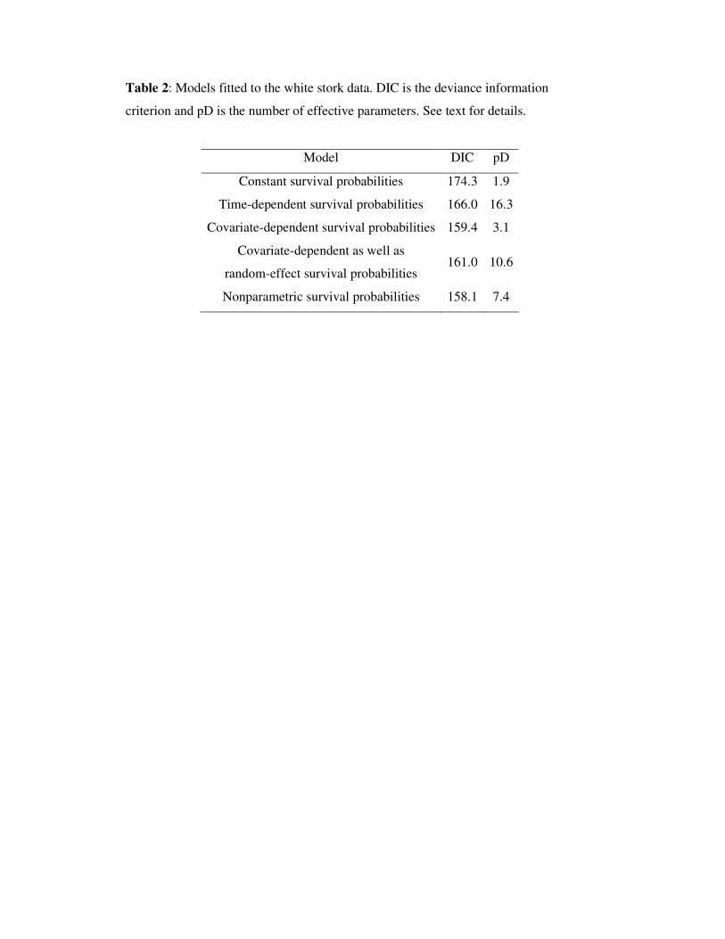
Table 2: Models fitted to the white stork data. DIC is the deviance information
criterion and pD is the number of effective parameters. See text for details.
Model DIC pD
Constant survival probabilities 174.3 1.9
Time-dependent survival probabilities 166.0 16.3
Covariate-dependent survival probabilities 159.4 3.1
Covariate-dependent as well as
random-effect survival probabilities 161.0 10.6
Nonparametric survival probabilities 158.1 7.4
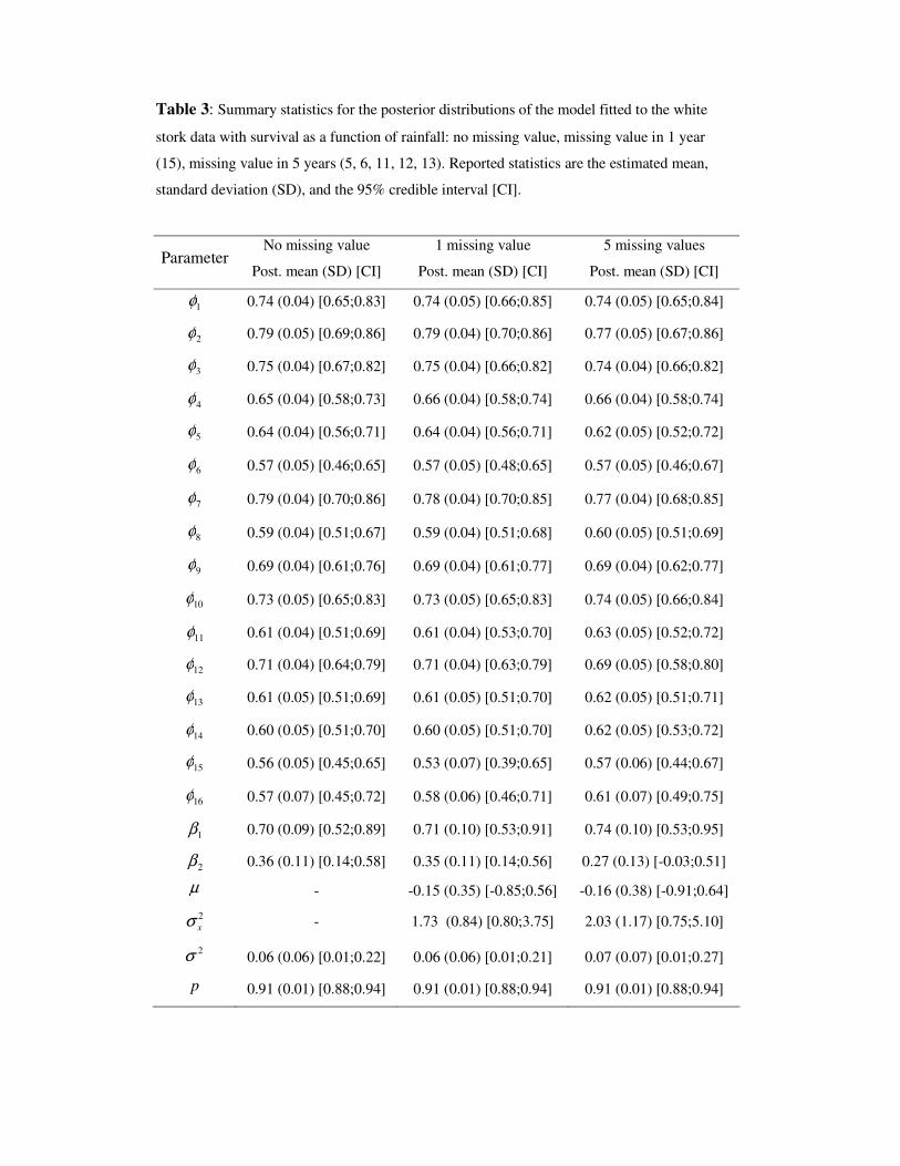
Table 3: Summary statistics for the posterior distributions of the model fitted to the white
stork data with survival as a function of rainfall: no missing value, missing value in 1 year
(15), missing value in 5 years (5, 6, 11, 12, 13). Reported statistics are the estimated mean,
standard deviation (SD), and the 95% credible interval [CI].
Parameter No missing value
Post. mean (SD) [CI]
1 missing value
Post. mean (SD) [CI]
5 missing values
Post. mean (SD) [CI]
1φ 0.74 (0.04) [0.65;0.83] 0.74 (0.05) [0.66;0.85] 0.74 (0.05) [0.65;0.84]
2φ 0.79 (0.05) [0.69;0.86] 0.79 (0.04) [0.70;0.86] 0.77 (0.05) [0.67;0.86]
3φ 0.75 (0.04) [0.67;0.82] 0.75 (0.04) [0.66;0.82] 0.74 (0.04) [0.66;0.82]
4φ 0.65 (0.04) [0.58;0.73] 0.66 (0.04) [0.58;0.74] 0.66 (0.04) [0.58;0.74]
5φ 0.64 (0.04) [0.56;0.71] 0.64 (0.04) [0.56;0.71] 0.62 (0.05) [0.52;0.72]
6φ 0.57 (0.05) [0.46;0.65] 0.57 (0.05) [0.48;0.65] 0.57 (0.05) [0.46;0.67]
7φ 0.79 (0.04) [0.70;0.86] 0.78 (0.04) [0.70;0.85] 0.77 (0.04) [0.68;0.85]
8φ 0.59 (0.04) [0.51;0.67] 0.59 (0.04) [0.51;0.68] 0.60 (0.05) [0.51;0.69]
9φ 0.69 (0.04) [0.61;0.76] 0.69 (0.04) [0.61;0.77] 0.69 (0.04) [0.62;0.77]
10φ 0.73 (0.05) [0.65;0.83] 0.73 (0.05) [0.65;0.83] 0.74 (0.05) [0.66;0.84]
11φ 0.61 (0.04) [0.51;0.69] 0.61 (0.04) [0.53;0.70] 0.63 (0.05) [0.52;0.72]
12φ 0.71 (0.04) [0.64;0.79] 0.71 (0.04) [0.63;0.79] 0.69 (0.05) [0.58;0.80]
13φ 0.61 (0.05) [0.51;0.69] 0.61 (0.05) [0.51;0.70] 0.62 (0.05) [0.51;0.71]
14φ 0.60 (0.05) [0.51;0.70] 0.60 (0.05) [0.51;0.70] 0.62 (0.05) [0.53;0.72]
15φ 0.56 (0.05) [0.45;0.65] 0.53 (0.07) [0.39;0.65] 0.57 (0.06) [0.44;0.67]
16φ 0.57 (0.07) [0.45;0.72] 0.58 (0.06) [0.46;0.71] 0.61 (0.07) [0.49;0.75]
1β 0.70 (0.09) [0.52;0.89] 0.71 (0.10) [0.53;0.91] 0.74 (0.10) [0.53;0.95]
2β 0.36 (0.11) [0.14;0.58] 0.35 (0.11) [0.14;0.56] 0.27 (0.13) [-0.03;0.51]
µ - -0.15 (0.35) [-0.85;0.56] -0.16 (0.38) [-0.91;0.64]
2
xσ - 1.73 (0.84) [0.80;3.75] 2.03 (1.17) [0.75;5.10]
2σ 0.06 (0.06) [0.01;0.22] 0.06 (0.06) [0.01;0.21] 0.07 (0.07) [0.01;0.27]
p 0.91 (0.01) [0.88;0.94] 0.91 (0.01) [0.88;0.94] 0.91 (0.01) [0.88;0.94]
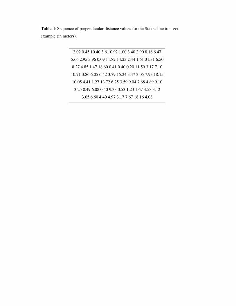
Table 4: Sequence of perpendicular distance values for the Stakes line transect
example (in meters).
2.02 0.45 10.40 3.61 0.92 1.00 3.40 2.90 8.16 6.47
5.66 2.95 3.96 0.09 11.82 14.23 2.44 1.61 31.31 6.50
8.27 4.85 1.47 18.60 0.41 0.40 0.20 11.59 3.17 7.10
10.71 3.86 6.05 6.42 3.79 15.24 3.47 3.05 7.93 18.15
10.05 4.41 1.27 13.72 6.25 3.59 9.04 7.68 4.89 9.10
3.25 8.49 6.08 0.40 9.33 0.53 1.23 1.67 4.53 3.12
3.05 6.60 4.40 4.97 3.17 7.67 18.16 4.08
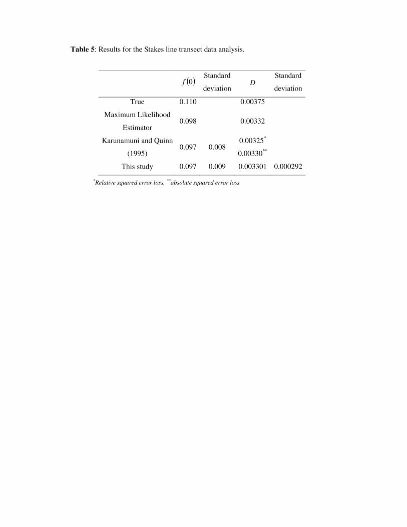
Table 5: Results for the Stakes line transect data analysis.
( )0f Standard
deviation D
Standard
deviation
True 0.110 0.00375
Maximum Likelihood
Estimator 0.098 0.00332
Karunamuni and Quinn
(1995) 0.097 0.008
0.00325*
0.00330**
This study 0.097 0.009 0.003301 0.000292
*Relative squared error loss,
**absolute squared error loss
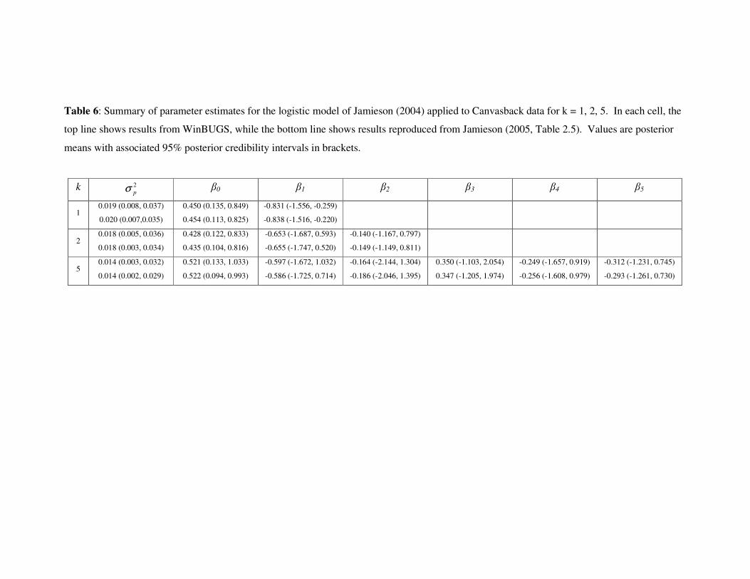
Table 6: Summary of parameter estimates for the logistic model of Jamieson (2004) applied to Canvasback data for k = 1, 2, 5. In each cell, the
top line shows results from WinBUGS, while the bottom line shows results reproduced from Jamieson (2005, Table 2.5). Values are posterior
means with associated 95% posterior credibility intervals in brackets.
k 2
pσ β0 β1 β2 β3 β4 β5
1 0.019 (0.008, 0.037)
0.020 (0.007,0.035)
0.450 (0.135, 0.849)
0.454 (0.113, 0.825)
-0.831 (-1.556, -0.259)
-0.838 (-1.516, -0.220)
2 0.018 (0.005, 0.036)
0.018 (0.003, 0.034)
0.428 (0.122, 0.833)
0.435 (0.104, 0.816)
-0.653 (-1.687, 0.593)
-0.655 (-1.747, 0.520)
-0.140 (-1.167, 0.797)
-0.149 (-1.149, 0.811)
5 0.014 (0.003, 0.032)
0.014 (0.002, 0.029)
0.521 (0.133, 1.033)
0.522 (0.094, 0.993)
-0.597 (-1.672, 1.032)
-0.586 (-1.725, 0.714)
-0.164 (-2.144, 1.304)
-0.186 (-2.046, 1.395)
0.350 (-1.103, 2.054)
0.347 (-1.205, 1.974)
-0.249 (-1.657, 0.919)
-0.256 (-1.608, 0.979)
-0.312 (-1.231, 0.745)
-0.293 (-1.261, 0.730)

48
Table 7: Posterior model probabilities for k = 0, …, 5 for the logistic model of 1
Jamieson (2004) applied to Canvasback data. 2
3
k WinBUGS Jamieson C code
0 0.279 0.265
1 0.685 0.697
2 0.034 0.036
3 0.002 0.002
4 0.000 0.001
5 0.000 0.000
4
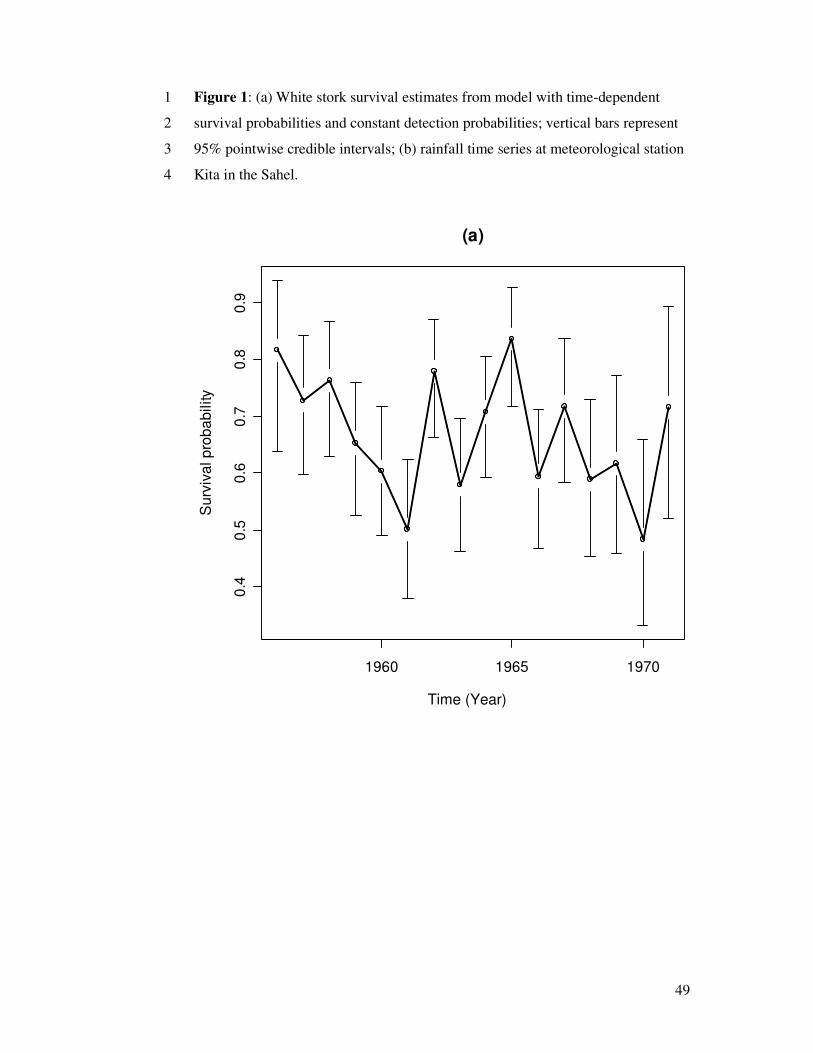
49
Figure 1: (a) White stork survival estimates from model with time-dependent 1
survival probabilities and constant detection probabilities; vertical bars represent 2
95% pointwise credible intervals; (b) rainfall time series at meteorological station 3
Kita in the Sahel. 4
1960 1965 1970
0.4
0.5
0.6
0.7
0.8
0.9
Time [Year, Year + 1]
Su
rviv
al p
rob
ab
ility
(a)
Time (Year)
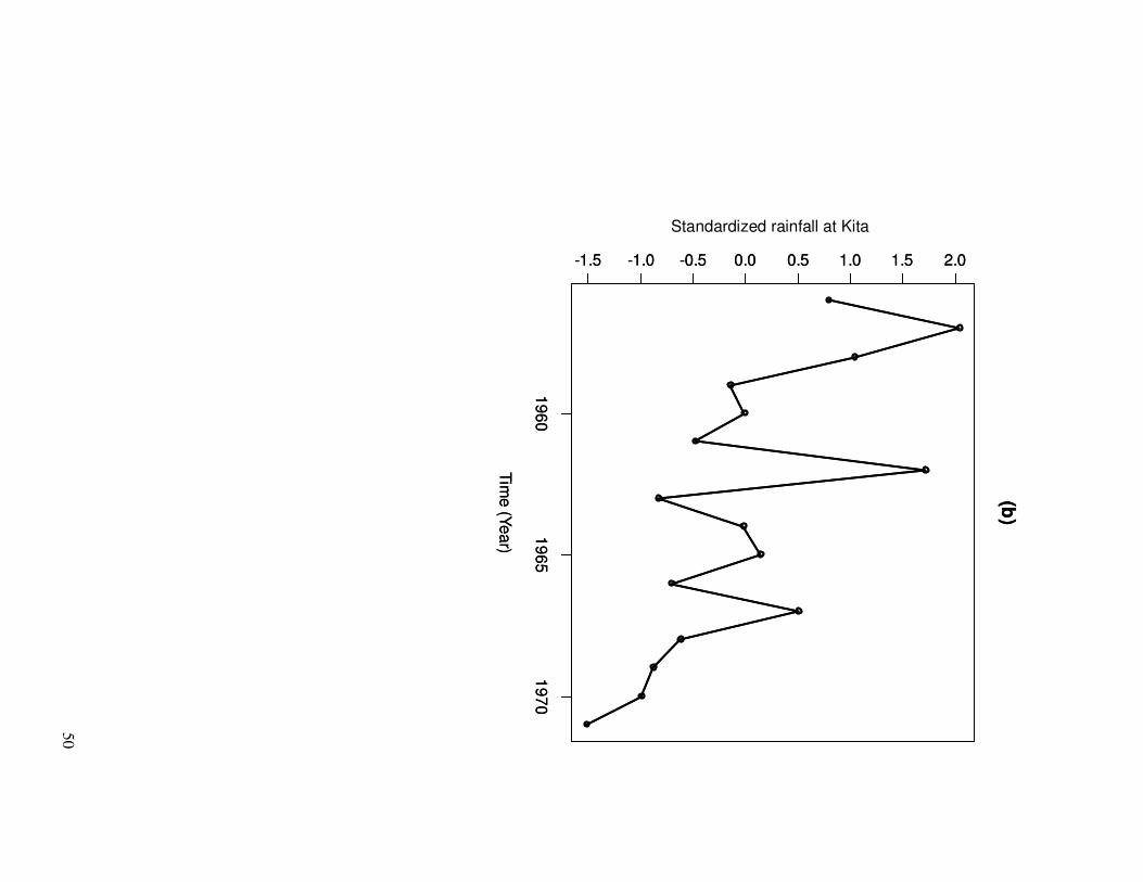
50
19
60
19
65
19
70
-1.5 -1.0 -0.5 0.0 0.5 1.0 1.5 2.0
Tim
e (Y
ea
r)
Pluviometry at Kita
(b)
Standardized rainfall at Kita
19
60
19
65
19
70
-1.5 -1.0 -0.5 0.0 0.5 1.0 1.5 2.0
Tim
e (Y
ea
r)
Pluviometry at Kita
(b)
Standardized rainfall at Kita
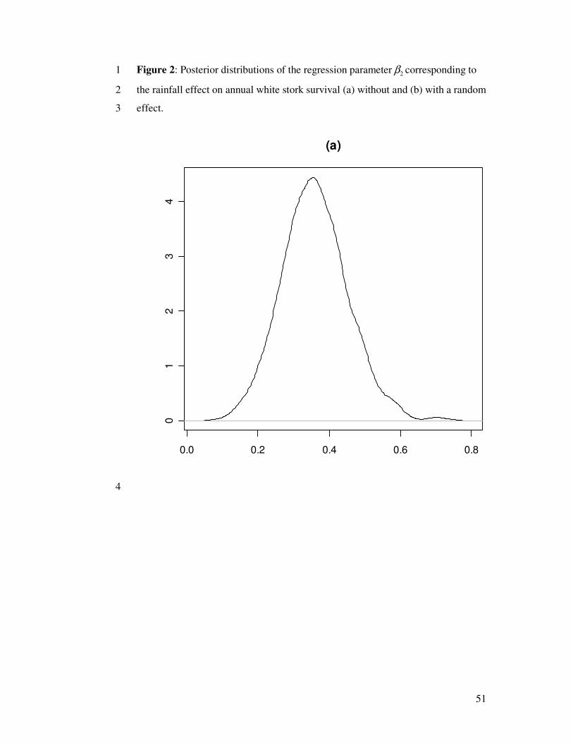
51
Figure 2: Posterior distributions of the regression parameter 2β corresponding to 1
the rainfall effect on annual white stork survival (a) without and (b) with a random 2
effect. 3
0.0 0.2 0.4 0.6 0.8
01
23
4
(a)
4

52
0.0 0.2 0.4 0.6 0.8
01
23
4
(b)
1
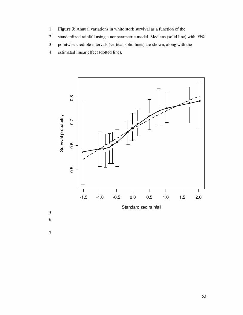
53
Figure 3: Annual variations in white stork survival as a function of the 1
standardized rainfall using a nonparametric model. Medians (solid line) with 95% 2
pointwise credible intervals (vertical solid lines) are shown, along with the 3
estimated linear effect (dotted line). 4
-1.5 -1.0 -0.5 0.0 0.5 1.0 1.5 2.0
0.5
0.6
0.7
0.8
Standardized rainfall
Su
rviv
al p
rob
ab
ility
5
6
7
Recommended