Yield Curve Predictorsof Foreign Exchange Returns∗
Andrew Ang†
Columbia University and NBER
Joseph S. Chen‡
UC Davis
Preliminary Incomplete Version: 4 September 2009Do not circulate
JEL Classification: E43, F31, F37, G15, G17Keywords: carry trade, exchange rates, predictability, term structure,
uncovered interest rate parity
∗We thank Bob Hodrick and Antti Ilmanen for helpful discussions.†Columbia Business School, 3022 Broadway 413 Uris, New York NY 10027, ph: (212) 854-9154;
email: [email protected]; WWW: http://www.columbia.edu/∼aa610.‡Graduate School of Management, University of California, Davis, One Shields Avenue, 3216 Gal-
lagher Hall, Davis, CA 95616; ph: (530) 752-2924; email: [email protected]; WWW: http://www.jc-finance.com
Yield Curve Predictors of Foreign Exchange Returns
Abstract
We find there is significant information in foreign countries’ yield curves that is useful
for predicting foreign exchange returns in the cross-section. This predictive information goes
beyond the violation of uncovered interest parity and the carry trade. We investigate cross-
sectional foreign exchange rate predictability using both a portfolio formation perspective and
a cross-sectional panel regression framework. Differences across countries of both the levels
of interest rates and the changes in interest rates have significant ability to forecast the cross-
section of future currency returns. Furthermore, we find additional predictive information in the
slope of the yield curve. Our results are consistent with no-arbitrage models that suggests factors
that determine the term structure of yields should also determine foreign exchange returns.
1 Introduction
In no-arbitrage models, the foreign exchange risk premium is driven by differences in risk
factors affecting the pricing kernels in each country.1 These factors are reflected in the term
structure of foreign and domestic bond prices and the conditional dynamics of yield curves over
time. The vast majority of studies examining the predictability of foreign exchange returns use
only the very shortest maturities of bond yields, like the differences between two countries in
their one-month or three-month interest rates (also called carry).2 However, it is well known
that there is more than one risk factor affecting interest rates and many modern term structure
models, like Dai and Singleton (2000) among many others, specify the pricing kernel to contain
at least three or more factors. Thus, the entire term structure of interest rates in each country and
their dynamic behavior over time should contain observable information in addition to short-
term interest rate differentials that affects foreign exchange returns.
Our paper emphasizes the restrictions on the joint behavior between currencies and term
structure of interest rates. The focus in this paper is to examine the predictive power of infor-
mation in the shapes and dynamics of the term structure for predicting future foreign exchange
returns. We take as a benchmark case the difference in short-term interest rates, which determine
the well-known violations from the uncovered interest rate parity (UIP) and the profitability of
the carry trade. Then, motivated from multi-factor term structure models, we examine several
other predictors constructed from the term structure of yields.
In particular, we document the predictive ability present in levels, changes and slopes of the
cross-section of yield curves. For instance, a simple currency portfolio constructed based on
changes in short-term interest rate differentials across countries yields an annualized Sharpe ra-
tio of 0.683 and exhibits no significant skewness. As a comparison, a simple currency portfolio
based on the levels of the short rate (the carry trade portfolio) yields an annualized Sharpe ratio
of 0.870, but exhibits significant negative skewness. A currency portfolio based on changes
in long-term bond yields also exhibit a substantial Sharpe ratio of 0.502. Moreover, these
portoflios are not significantly correlated with each other. We verify this predictability in a
panel regression framework as well.
1 Earliest paper to note this relation is Fama (1984).2 There is a huge literature documenting deviations from the Unbiasedness Hypothesis where differences in
short rates, or equivalently forward rates, predict future exchange rates. Hodrick (1988), Lewis (1995) and Engel
(1996) are survey articles of the early literature. Sarno (2005) is a more recent update. This literature is exclusively
time-series studies, whereas we investigate the cross-sectional relations.
1
One notable feature of our empirical analysis is that we take a cross-sectional approach
to examine foreign exchange predicability as opposed to the more commonly examined time-
series predictability regressions in the literature. The cross-sectional approach lets us get closer
to examining foreign exchange predictability in a no-arbitrage framework. We show our for-
eign exchange predictability using both a portfolio formation framework and a cross-sectional
panel regression. Our results readily illustrates what a hypothetical arbitraguer would face. In
contrast, a time-series approach has the disadvantage that it does not necessarily translate to a
practical implementation by an arbitraguer.
To provide a motivating theoretical framework for interpreting our empirical results, we
illustrate a series of models in which factors that determine the term structure also impacts the
foreign exchanges returns. We consider various models commonly used in the term structure
literature and illustrate the models’ implications on foreign currency exchange returns. Our
main message is that any factor that affects the term structure of yields may also forecast foreign
exchange rates. We emphasize the predictive ability of the levels, the changes, and the slopes
of the yield curve. However, we do not take a stance on which model, if any, fits the data. We
only note that our foreign exchange predictability results we find in data are still consistent with
no-arbitrage pricing.
Our paper is structured as follows. Section 2 provides a brief summary of related paper. We
provide a motivation theoretical framework for our empirical investigation in Section 3. Section
4 describes our data and provides summary statistics. Section 5 considers currency returns from
a portfolio framework. We present our main empirical results in Section 6. Section 7 concludes.
2 Related Literature
This section is incomplete
Different horizons – only examined previously in time-series contexts, e.g. Chinn (2006).
FX portfolios – Burnside et al. (2006), Lustig, Roussanov and Verdelhan (2008)
Balduzzi et al. (1996) three factor model – level, central tendency, conditional volatility
Examined in the context of a general affine model by Dai and Singleton (2000).
Macro predictors of the yield curve – ignore. Ref Ang and Piazzesi (2003). Taylor rules in
ER’s literature Molodtsova and Papell (2008), Wang and Wu (2009). Other macro fundamen-
tals, long history. Engel, Mark and West (2007) differentials of macro variables. Cite Engle and
West (2005).
2
Literature on no-arbitrage term structure models of currency pricing Fama (1984), Backus,
Foresi and Telmer (2001), Brandt and Santa-Clara (2002 , Hodrick and Vassalou (2002), Bansal
(1997), Ahn (2004), Dong (2006), Graveline (2006), All two-country models.
Most related to Boudoukh, Richardson and Whitelaw (2006) – time series only on long-
maturity forward rates, equivalent to using information in long yields. Also Chen and Tsang
(2009) using level, slope and curvature constructed from splines.
Underreaction story? Burnside, Eichenbaum and Rebelo (2007) and Gourinchas and Tornell
(2004)
Changes in short rates – Ilmanen and Sayood (1998, 2002). In industry models, see John
Normand, JP Morgan.
Look at skewness of portfolios – Jurek (2008), Brunnermeier, Nagel and Pedersen (2009)
3 Motivating Framework
Under no-arbitrage conditions there exists a stochastic discount factor or pricing kernel, Mt+1,
which prices any payoff Pt+1 at time t+ 1 so that the price Pt at time t satisfies
Pt = Et[Mt+1Pt+1]. (1)
In particular, the price of a n-period zero coupon bond, P (n)t , is given by
P(n)t = Et[Mt+1P
(n−1)t+1 ] (2)
and the price of the one-period bond is simply the one-period risk-free rate, rt,
P(1)t = exp(−rt) = Et[Mt+1]. (3)
The pricing kernel embodies risk premiums, which potentially vary over time. Suppose the
domestic pricing kernel takes the form
Mt+1 = exp(−rt − 1
2λ2t − λtεt+1
), (4)
where λt is a time-varying price of risk which prices the shock to the short rate, εt+1. In our
analysis we specify all our shocks to be N(0, 1) and uncorrelated with each other. The price of
risk, λt, is potentially driven by multiple factors. Time-varying prices of risk give rise to time-
varying risk premia on long-term bonds. An enormous body of previous research has found
that priced risk factors include interest rate factors like the level and slope of the yield curve
3
and other yield curve variables, in addition to macro variables like inflation and output (see the
summary of affine term structure models by Piazzesi, 2003). In our exposition we concentrate
on yield curve factors.
We assume a similar pricing kernel in foreign country i:
M it+1 = exp
(−rit − 1
2(λit)
2 − λitεit+1
). (5)
The foreign pricing kernel prices all bonds in the foreign country through a similar relation to
equation (2),
Pi,(n)t = Et[M
it+1P
i,(n−1)t+1 ]
where P i,(n)t is the time t price of the foreign n-period zero coupon bond denominated in foreign
currency.
Let the spot exchange rate Sit at time t express the amount of U.S. dollars per unit of foreign
currency i. Increases in Sit represent an appreciating foreign currency relative to a depreciating
US dollar. Under complete markets the exchange rate change is the ratio of the pricing kernels
in the foreign and domestic country:
Sit+1
Sit=M i
t+1
Mt+1
, (6)
which is derived by many authors including Bekaert (1996), Bansal (1997), and Backus, Foresi
and Telmer (2001). We denote natural logarithms of our variables as sit+1 = logSit+1, mit+1 =
logM it+1 and mt+1 = logMt+1 The rate of foreign currency appreciation relative to US dollar ,
∆sit+1, is given by
∆sit+1 = sit+1 − sit = mit+1 −mt+1
= rt − rit + 12(λ2
t − (λit)2) + λtεt+1 − λitεit+1. (7)
Under this setting the foreign exchange risk premium of the ith currency, rpit, is half the differ-
ence in the spread of the conditional variances of the domestic and foreign pricing kernels:
rpit = Et(∆sit+1 + rit − rt) = 1
2(λ2
t − (λit)2). (8)
The risk premium, rpit, is the expected return to purchasing a foreign currency, investing the
proceeds in a foreign bond for one period earning the foreign interest rate, and then converting
back to domestic currency, which is given by Et[∆sit+1 + rit], in excess of investing in the US
one-period bond, which is given by rt. Note that uncovered interest rate parity (UIP) assumes
that the right-hand side of equation (8) is zero. In UIP, if foreign interest rate is greater than
4
the US interest rate, rit > rt , then the foreign currency is expected to depreciate. However,
equation (8) shows that any factor affecting the prices of domestic or foreign bonds potentially
has the ability to predict foreign exchange excess returns.3
Equation (8) is the motivating framework for examining the predictability of various factors
which drive risk premia in domestic or foreign bond markets, which may also predict foreign
exchange risk premia. We begin by showing how the standard carry trade assumes a one-factor
model for the price of risk which is the same as the short rate in Section 3.1. Then, in sections
3.2-3.4 we extend the framework to allow for multiple factors driving the prices of risk. In
this richer environment long-term bond yields and other statistics capturing the dynamics of
the yield curve may be simple instruments to capture these additional risk factors. Our goal is
not to develop a complicated term structure model that jointly prices domestic and foreign term
structures and exchange rates, but rather to provide motivation of how various transformations
of the yield curve may serve as approximations of factors driving risk premia. We summarize
in Section 3.5.
3.1 Differentials in Short Rates
We start with a simple one-factor model of the yield curve, which dates back to at least Vasicek
(1977). We parameterize the short rate in the U.S. and foreign country as
rt+1 = θ + ρrt + σrεr,t+1
rit+1 = θ + ρrit + σrεit+1 (9)
where for simplicity we assume the same parameters in the U.S. and the foreign country.
Long-term bonds reflect the risk premiums. The price of a two-period bond is given by
P(2)t = Et[Mt+1Et+1[Mt+2]]
= Et
[exp
(−rt − 1
2λ2t − λtεr,t+1 − rt+1
)](10)
which simplifies to
P(2)t = exp(1
2σ2r − rt − θ − ρrt − σrλt).
The yield on the two-period bond is
y(2)t = −1
2logP
(2)t = −1
4σ2r + 1
2(rt + θ + ρrt) + 1
2σrλt, (11)
3 In incomplete markets it is possible that certain factors affect only exchange rate returns and not domestic or
foreign bond prices. For example, Brandt and Santa-Clara (2002) incorporate an additional risk factor to match
exchange rate volatility but this factor is not priced and does not affect foreign exchange risk premiums.
5
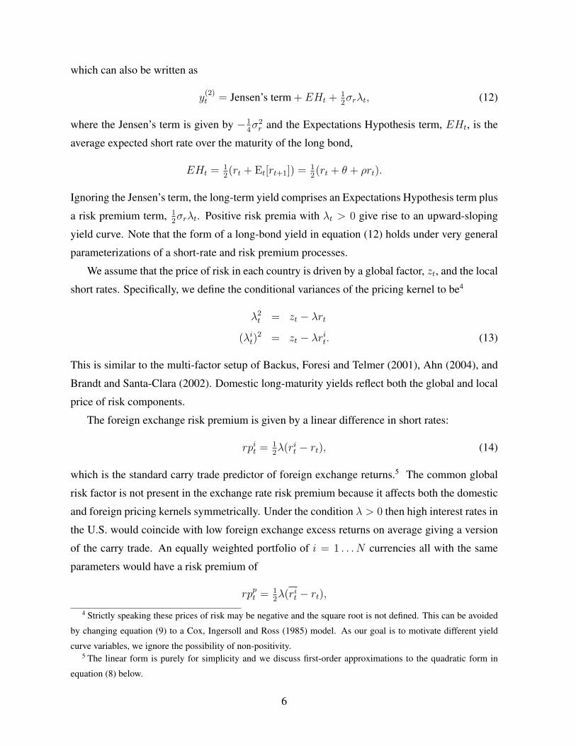
which can also be written as
y(2)t = Jensen’s term + EHt + 1
2σrλt, (12)
where the Jensen’s term is given by −14σ2r and the Expectations Hypothesis term, EHt, is the
average expected short rate over the maturity of the long bond,
EHt = 12(rt + Et[rt+1]) = 1
2(rt + θ + ρrt).
Ignoring the Jensen’s term, the long-term yield comprises an Expectations Hypothesis term plus
a risk premium term, 12σrλt. Positive risk premia with λt > 0 give rise to an upward-sloping
yield curve. Note that the form of a long-bond yield in equation (12) holds under very general
parameterizations of a short-rate and risk premium processes.
We assume that the price of risk in each country is driven by a global factor, zt, and the local
short rates. Specifically, we define the conditional variances of the pricing kernel to be4
λ2t = zt − λrt
(λit)2 = zt − λrit. (13)
This is similar to the multi-factor setup of Backus, Foresi and Telmer (2001), Ahn (2004), and
Brandt and Santa-Clara (2002). Domestic long-maturity yields reflect both the global and local
price of risk components.
The foreign exchange risk premium is given by a linear difference in short rates:
rpit = 12λ(rit − rt), (14)
which is the standard carry trade predictor of foreign exchange returns.5 The common global
risk factor is not present in the exchange rate risk premium because it affects both the domestic
and foreign pricing kernels symmetrically. Under the condition λ > 0 then high interest rates in
the U.S. would coincide with low foreign exchange excess returns on average giving a version
of the carry trade. An equally weighted portfolio of i = 1 . . . N currencies all with the same
parameters would have a risk premium of
rppt = 12λ(rit − rt),
4 Strictly speaking these prices of risk may be negative and the square root is not defined. This can be avoided
by changing equation (9) to a Cox, Ingersoll and Ross (1985) model. As our goal is to motivate different yield
curve variables, we ignore the possibility of non-positivity.5 The linear form is purely for simplicity and we discuss first-order approximations to the quadratic form in
equation (8) below.
6
where rit = 1N
∑rit is the average short rate across countries.
Note that although long-term yields reflect the risk premium in equation (11), long-term
bonds have no extra predictive power for exchange rate returns above short rates differentials in
equation (14). In fact, using long-term bonds would lead to less predictive power for exchange
rate returns because long-term bonds embed both the common risk factor zt and the local short-
rate factors whereas only local risk factors matter for exchange rate determination. In this
simple setting only differences in short rates are useful for predicting foreign exchange returns.
We now turn to a richer specification for risk premia where there will be a role for long-term
bonds and other yield curve transformations in predicting exchange rates.
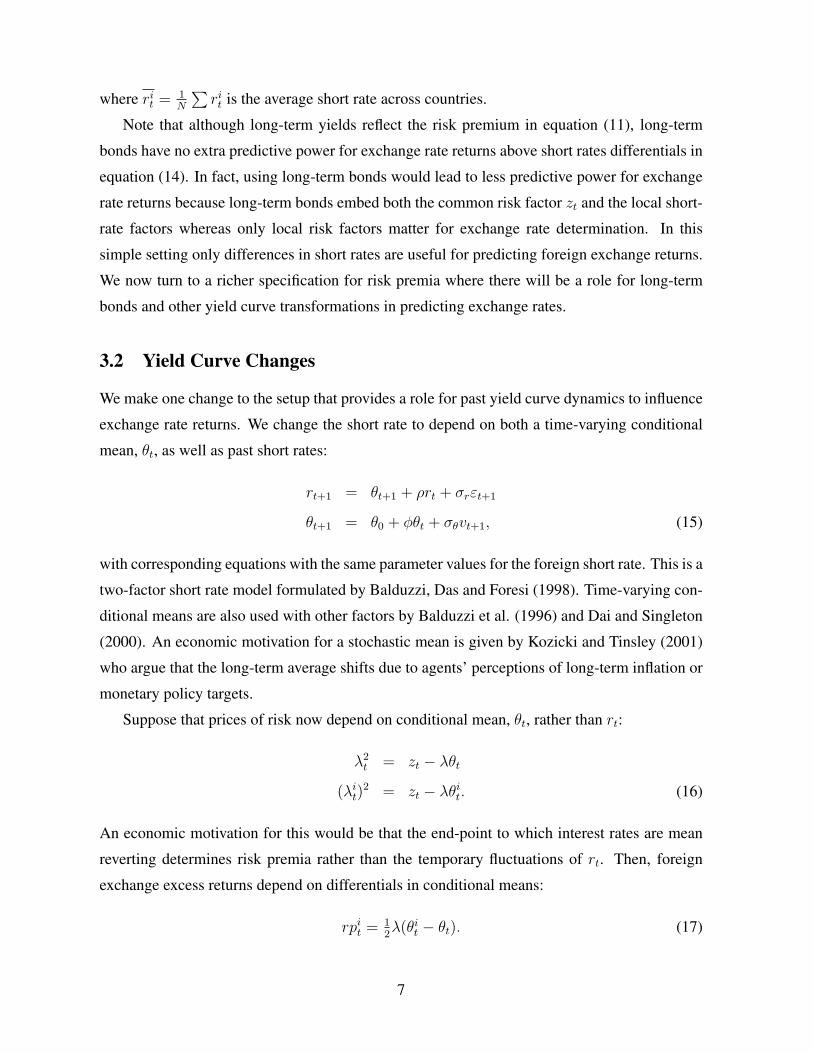
3.2 Yield Curve Changes
We make one change to the setup that provides a role for past yield curve dynamics to influence
exchange rate returns. We change the short rate to depend on both a time-varying conditional
mean, θt, as well as past short rates:
rt+1 = θt+1 + ρrt + σrεt+1
θt+1 = θ0 + φθt + σθvt+1, (15)
with corresponding equations with the same parameter values for the foreign short rate. This is a
two-factor short rate model formulated by Balduzzi, Das and Foresi (1998). Time-varying con-
ditional means are also used with other factors by Balduzzi et al. (1996) and Dai and Singleton
(2000). An economic motivation for a stochastic mean is given by Kozicki and Tinsley (2001)
who argue that the long-term average shifts due to agents’ perceptions of long-term inflation or
monetary policy targets.
Suppose that prices of risk now depend on conditional mean, θt, rather than rt:
λ2t = zt − λθt
(λit)2 = zt − λθit. (16)
An economic motivation for this would be that the end-point to which interest rates are mean
reverting determines risk premia rather than the temporary fluctuations of rt. Then, foreign
exchange excess returns depend on differentials in conditional means:
rpit = 12λ(θit − θt). (17)
7
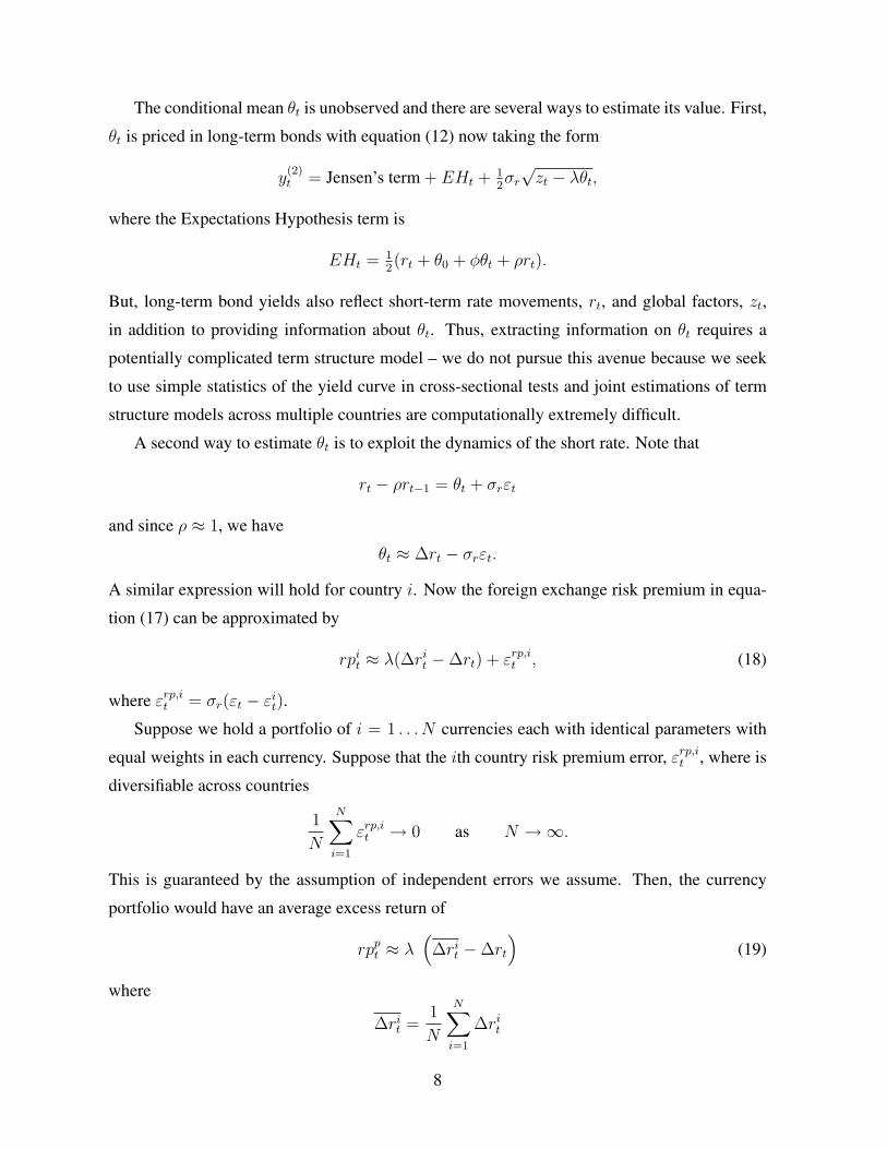
The conditional mean θt is unobserved and there are several ways to estimate its value. First,
θt is priced in long-term bonds with equation (12) now taking the form
y(2)t = Jensen’s term + EHt + 1
2σr√zt − λθt,
where the Expectations Hypothesis term is
EHt = 12(rt + θ0 + φθt + ρrt).
But, long-term bond yields also reflect short-term rate movements, rt, and global factors, zt,
in addition to providing information about θt. Thus, extracting information on θt requires a
potentially complicated term structure model – we do not pursue this avenue because we seek
to use simple statistics of the yield curve in cross-sectional tests and joint estimations of term
structure models across multiple countries are computationally extremely difficult.
A second way to estimate θt is to exploit the dynamics of the short rate. Note that
rt − ρrt−1 = θt + σrεt
and since ρ ≈ 1, we have
θt ≈ ∆rt − σrεt.
A similar expression will hold for country i. Now the foreign exchange risk premium in equa-
tion (17) can be approximated by
rpit ≈ λ(∆rit −∆rt) + εrp,it , (18)
where εrp,it = σr(εt − εit).
Suppose we hold a portfolio of i = 1 . . . N currencies each with identical parameters with
equal weights in each currency. Suppose that the ith country risk premium error, εrp,it , where is
diversifiable across countries
1
N
N∑i=1
εrp,it → 0 as N →∞.
This is guaranteed by the assumption of independent errors we assume. Then, the currency
portfolio would have an average excess return of
rppt ≈ λ(
∆rit −∆rt
)(19)
where
∆rit =1
N
N∑i=1
∆rit
8
is the average change in short rates across countries. Intuitively, short rate changes provide
information about persistent time-varying conditional means. If these factors are priced then
ranking on changes in short rates across currencies may lead to differences in expected returns.
In our empirical work we also consider changes in long-term bond yields and term spreads,
which we now motivate in terms of levels.
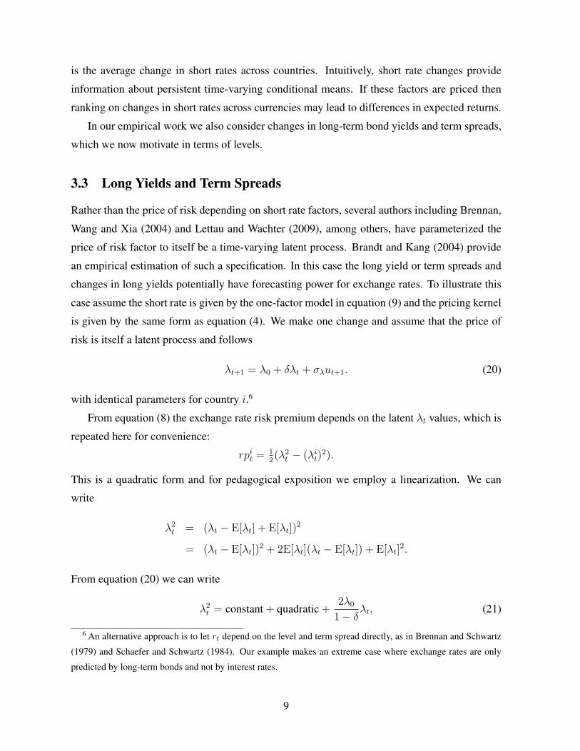
3.3 Long Yields and Term Spreads
Rather than the price of risk depending on short rate factors, several authors including Brennan,
Wang and Xia (2004) and Lettau and Wachter (2009), among others, have parameterized the
price of risk factor to itself be a time-varying latent process. Brandt and Kang (2004) provide
an empirical estimation of such a specification. In this case the long yield or term spreads and
changes in long yields potentially have forecasting power for exchange rates. To illustrate this
case assume the short rate is given by the one-factor model in equation (9) and the pricing kernel
is given by the same form as equation (4). We make one change and assume that the price of
risk is itself a latent process and follows
λt+1 = λ0 + δλt + σλut+1. (20)
with identical parameters for country i.6
From equation (8) the exchange rate risk premium depends on the latent λt values, which is
repeated here for convenience:
rpit = 12(λ2
t − (λit)2).
This is a quadratic form and for pedagogical exposition we employ a linearization. We can
write
λ2t = (λt − E[λt] + E[λt])
2
= (λt − E[λt])2 + 2E[λt](λt − E[λt]) + E[λt]
2.
From equation (20) we can write
λ2t = constant + quadratic +
2λ0
1− δλt, (21)
6 An alternative approach is to let rt depend on the level and term spread directly, as in Brennan and Schwartz
(1979) and Schaefer and Schwartz (1984). Our example makes an extreme case where exchange rates are only
predicted by long-term bonds and not by interest rates.
9
where the quadratic term is (λt − E[λt])2. Assuming the quadratic variation is small then
λ2t ≈ constant +
2λ0
1− δλt,
and we can approximate the risk premium as
rpit =λ0
1− δ(λt − λit). (22)
Exchange rate returns depend on prices of risk, but these prices of risk are not observed in
short rate dynamics. In fact, in this stylized case foreign exchange excess returns cannot be
predicted by short rates. Prices of risk show up in long-bond prices or term spreads, which take
the form
y(2)t = −1
4σ2r + 1
2((1 + ρ)rt + θ) + 1
2σrλt
for the long yield and
y(2)t − rt = −1
4σ2r + 1
2((1− ρ)rt + θ) + 1
2σrλt
for the term spread. In particular, since ρ ≈ 1, the term spread provides a direct estimate of λt:
y(2)t − rt ≈ constant + 1
2σrλt.
Thus, we can obtain an estimate of the exchange rate risk premium using term spreads:
rpit ≈2λ0
σr(1− δ)
((y
(2),it − rit)− (y
(2)t − rt)
). (23)
3.4 Interest Rate Volatility
We finally consider a case where interest rate volatility predicts foreign exchange risk premiums.
We take a two-factor model of the short rate where volatility is stochastic:
rt+1 = θ + ρrt +√vtεt+1
vt+1 = v0 + κvt + σv√vtηt+1. (24)
This is the model of Longstaff and Schwartz (1992) where the second factor is identified with
the conditional volatility of the short rate. A similar specification is used by Balduzzi et al.
(1996).
We let the pricing kernel now price fluctuations in the short rate volatility, ηt+1. Specifically,
we assume
Mt+1 = exp(−rt − 1
2λ2vvt − λv
√vtηt+1
), (25)
10
where we shut off any potential pricing of risk for regular short rate shocks, εt+1, to highlight the
role of volatility. Assuming country i has the same parameters, the exchange rate risk premium
is then given by
rpit = 12(λ2
v(vt − vit)). (26)
Thus, interest rate volatility potentially may affect foreign exchange returns.
3.5 Summary
In summary, the expected return for investing in foreign currencies depends on the spread in
conditional volatilities of each country’s stochastic discount factor. Conditional volatility of a
country’s stochastic discount factor affects the term structure of yields. Therefore, any factor
that affects the domestic term structure of yields may potentially also forecast foreign exchange
risk premiums. In addition to differential spreads in short rates, which is the traditional carry
trade, foreign exchange returns may potentially be predicted by changes in interest rates, long-
bond yields and term spreads, and interest rate volatility. We now examine the predictive power
in the cross section of these various term structure factors.
4 Data and Summary Statistics
4.1 Data
The data used in our analysis consists of a panel of 22 foreign currencies that are foreign relative
to the US. The currencies are divided into a set of G10 currencies (Australia, Canada, Switzer-
land, Germany, France, United Kingdom, Japan, Norway, New Zealand and Sweden) and a set
of non-G10 developed countries (Austria, Belgium, Denmark, Spain, Finland, Greece, Hong
Kong, Ireland, Italy, Netherlands, Portugal, Singapore).7 During the sample period we study,
the Euro was introduced and many currencies became defunct. To account for the introduction
of the Euro, we eliminate a currency once it joins the European single currency, with one ex-
ception. Since the Euro itself is a valid currency, we splice the data for Germany with the data
for Euro. Germany is the country with the largest GDP among the countries in the Euro, hence
we consider the German Deutsche Mark to be representative of the Euro.
7 In out study, a country is developed if it was considered ”developed” by Morgan Stanley Capital International
(MSCI) as of June 2007.
11
We gather short-term and long-term interest rate variables from Global Financial Data at a
monthly frequency. For our analysis, we collect short-term interest rates that currency traders at
major financial institutions might realistically trade at. So we use the interbank deposit rates as
our preferred measure of short rate. For each of our currencies, we take the one-month London
interbank offered rates (LIBOR) or equivalent interbank offered rates traded elsewhere. If an
interbank offered rate is not available for a currency, we supplement the data with that country’s
3-month government bill rate, also obtained from Global Financial Data.8 We denote the short
rate as rit. We also collect long-term interest rate using the 10-year government bond, where
available. If the 10-year government bond rate is not available, we use the 5-year government
bond rate.9 We denote the long-term interest rate as yit and refer to it as ’long rate’. To ensure
that at least 6 currencies are represented among the G10 currencies, we begin our sample in
January 1979. Our sample ends in May 2007 and represents 341 months in total.
We also convert our interest rate variables to interest rates relative to US interest rates.10 We
also collect US dollar LIBOR rates, denoted rt and US 10-year constant maturity government
bond rate, denoted yt. These interest rate differentials, rit−rt and yit−yt, are our main predictive
variables of interest. We also compute term spread differentials defined as (yit − yt) − (rit −rt), and refer to it as the ’term spread’. Finally, we compute monthly changes in interest rate
differentials, denoted as ∆(rit − rt), ∆(yit − yt) and ∆ [(yit − yt)− (rit − rt)]For each currency, we obtain the end-of-month exchange rate in terms of dollar price of one
unit of foreign currency from Thomson Financial’s Datastream International, which we denote
as Sit . We define excess FX return on currency i over the next month, denoted Πit+1, as
Πit+1 = Sit+1/S
it(1 + rit)− (1 + rt). (27)
Note that this is the profit from borrowing one USD at rt to purchase 1/Sit units of foreign
currency i and depositing the proceeds at rit.
8 G10 currencies for which we used the 3-month government bill rates to increase sample length are AUD,
CAD, NZD and SEK. Among non-G10 developed countries, they are ATS, ESP, ITL, NLG, PTE and SGD.9 G10 currencies for which we used the 5-year government bond rates are AUD, CAD, CHF, FRF, NZD and
SEK. Among non-G10 developed countries, they are ATS, BEF, DKK and GRD.10 The portfolio strategies below takes zero position in the US dollar and all of our regression specification
includes time-fixed effects. Therefore, subtracting the US interest rate has no impact on our analysis.
12
4.2 Summary Statistics
We begin by presenting some basic features of data to help guide our empirical design. Table 1
shows means and sample ranges of our variables for the G10 currencies in Panel A, and for non-
G10 currencies in Panel B. Our currency returns are express in terms of percent per month. For
example, investing in Australian dollar financed by US dollar and rebalancing every month has
resulted in a net profit of 0.135% per month, or 1.62% per year. During this period Australian
dollar interest rate was on average higher than the US dollar rate by 0.181% per month, or 2.17%
per year. In this period, the Australian dollar depreciated against the US dollar by approximately
this difference, but the trade was profitably because of the interest earned. The average monthly
change in the short rate was 0.103 basis points per month, indicating Australian interest rate
rose relative tot he US interest rate slightly over this period. Looking at the long bond rate and
its changes depicts a similar history.
Note among the G10 currencies, currencies with lower short rate than the US dollar (CHF,
DEM and JPY) tend to produce negative future excess currency returns. This positive relation
is the main driver of the carry trade. Panel A of Table 2 formally looks at this pattern in terms
of correlations between time-series averages of excess currency return and time-series averages
of predictive yield curve variables. The positive coorelation between average excess currency
return and average short rate differential exist across all developed countries, but it is much
more pronounced when only the G10 currencies are considered. However, when we look at the
relation with average changes in interest rates and average excess currency returns, it seems to
be a negative relation.
While Panel A of Table 2 looks at relationships of means across currencies, it does not say
anything about relationships of these variables across time. Panel B of Table 2 gives us a glimpse
of the time-series relationship by showing the correlations of our variables in a pooled sample,
where the variables have been de-meaned by country. In time-series, each of our yield curve
predictive variables are positively correlated with future excess currency return. We formally
examine this in our regressions later. Also note that while levels short-term and long-term
interest rates tend to be very highly correlated, the changes in these variables are not.
Figure 2 plots the short rate for all currencies in time-series. There are a couple of features
that are worthwhile noting. First, many currencies have experienced periods of crisis. In 1992
a financial crisis swept through much of Europe affecting DKK, FIM, IEP, NOK and SEK
particularly hard, but also ESP and FRF. AUD and NZD experienced persistently high interest
rate differential in late 1980’s. Notably, financial turmoil seems to be norm for GRD and ITL
13
for much of our sample. Second, there has been a regime change in cross-currency variation in
interest rate differential. In particular there appears markedly lower variation in interest rates
since the late 1990’s. Finally, there are numerous entries and exists of currencies, especially
with the introduction of the Euro. We will be mindful of controlling for these features of the
data in designing our portfolio formations and regression specifications.
5 Portfolio Results
We begin by exploring the relation between excess currency returns and yield curve predictors
from a portfolio perspective first. We start by examining the standard carry traded used by prac-
titioners and consider using alternative predictive variables from the term structure of interest
rates. Since the standard carry trade is essentially based on indicator functions, we consider an
alternative portfolio specification that is closer to running a regression in spirit. All of our port-
folio results are from the point of view of a currency trader in the US. We assume that the trader
is able to transact all developed country currencies at no cost and is able to borrow and deposit
at the prevailing interbank rates. Furthermore, we assume that the trader takes no position in
his home currency. Hence, all portfolios considered take long and short positions in currencies,
with appropriate foreign deposits and foreign financing, but has zero holdings on the US dollar.
5.1 The Benchmark Carry Trade
The basic carry trade ranks currencies by the short rate differentials. The carry trade entails
purchasing currencies with high interest rates and selling currencies with low interest rates.
Generally, currencies with the highest (lowest) one-third values of interest rates are purchased
(sold). Among the purchases and the sales, the standard carry trade takes equal positions.
Hence, if there are ten currencies to choose from, the carry trade buys the highest three interest
currencies and sell the lowest three interest rate currencies with equal weights. These portfolios
are reevaluated and rebalanced each month. Note that from the point of view of a carry trade
based in the US, the net holdings of US dollar is zero. The standard carry trade is often based
on only the G10 currencies, but can be expanded to include additional currencies.
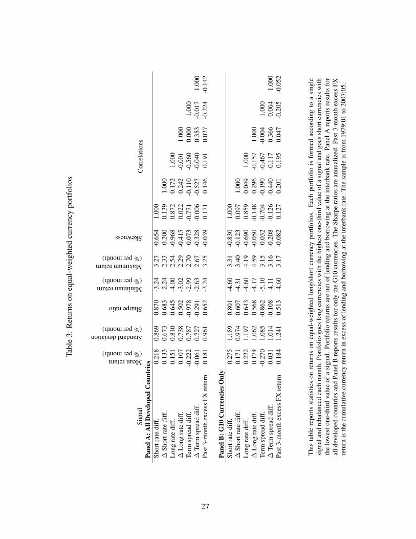
The summary statistics of our currency portfolios are presented in Table 3. Panel A consid-
ers the portfolios formed across all 22 developed country currencies while Panel B considers the
portfolios formed across only the G10 currencies. For each portfolio, we compute one-month
holding period returns and report their means and standard deviations. Since these portfolios are
14
zero cost positions, the returns can be thought of as profits on purchasing one US dollar worth of
high signal foreign currencies and borrowing one US dollar worth of low signal currencies. We
also report annualized Sharpe ratio, which is the ratio of means and standard deviations, scaled
by the square root of 12. Finally, we report minimum, maximum, and skewness of portfolio
returns and their correlations.
The first row of each panel describes the portfolio returns of the carry trade. When the trade
is conducted across all developed country currencies, the carry trade has averaged a return of
0.218% per month with a standard deviation of 0.869% per month. This translates to an impres-
sive annualized Sharpe ratio of 0.870. The results are mostly similar when only G10 currencies
are used. The average return is higher with only the G10 currencies, but the corresponding
Sharpe ratio is slightly lower. Since short rate differentials are very persistent, these portfolios
tend to have low monthly turnover. However, it is well known that these carry trade portfolio
returns have negative skewness and are prone to large losses. This tendency is more noticeable
when only G10 currencies are used.
5.2 Other Equal-Weighted Currency Portfolios
We now investigate if other parts of the yield curve has predictive information about future
currency returns in a portfolio framework. We construct additional currencies portfolios in the
same manner as the carry trade portfolios. However, rather than using the short rate differentials,
we also consider other signals as predictors of future currency returns. Specifically, we consider
the one-month changes in the short rate differentials, the long bond rate differentials, and the
one-month changes in the long bond rate differentials. To help separate the effects of the slope
of the yield curve from the level of the yield curve, we also look at the term spread differentials
and their one-month changes. As another benchmark, we also consider a currency momentum
portfolio, which is common in practice. The currency momentum portfolio uses information
in past currency returns and we use the past 3-month cumulative excess currency return as the
signal.
The second row of each panel of Table 3 shows the equal-weighted portfolio returns based
on changes in the short rate differentials. Across all developed country currencies, this trade
has averaged a return of 0.133% per month with a standard deviation of 0.673% per month.
This translates to an annualized Sharpe ratio of 0.683, which is large. The values are similar
when only G10 currencies are used. Unlike the carry trade, however, using changes in the
short rate leads to portfolio with higher turnover, but it leads to a portfolio without proneness to
15
large losses. In fact, when all developed country currencies are used, this portfolio has positive
skewness. Moreover, the correlation with carry trade returns is low at 0.139. In fact, a naive
strategy consisting of fifty-percent of this portfolio and fifty-percent in the carry trade portfolio
leads to a strategy with a Sharpe ratio of around 1.1.
The third and fourth rows in Table 3 show the portfolio returns when the long rate differen-
tials are used instead of the short rate differentials, in terms of both levels and changes. Figure
3 shows the time-series of cumulative returns on portfolios considered so far. Notice that using
the long rate leads to a portfolio with similar characteristics as the carry trade. In fact, the cor-
relation of this portfolio’s return with carry trade return is 0.872. Hence the levels of long rate
appears to have the same predictive information as the levels of short rate. However, the same
does not appear to be the case for portfolio based on changes in long rate differentials. This
portfolio produces a Sharpe ratio of 0.502, which is still significant. However, the correlations
with other portfolios we’ve considered are low to modest. The correlation of this portfolio with
the portfolio based on changes in the short rate differential is a modest 0.242. Hence there
appears to be some predictive information content in changes in the yield curve.
To organize the information about the yield curve differently, we fifth and sixth rows of
Table 3 show the portfolio returns based on levels and changes of the term spread. These
portfolios produce negative Sharpe ratios, so they should be reversed. That is, currencies with
low (or negative) term spread should be purchased and currencies with high slope of the yield
curve should be sold. Interestingly, combining the short rate differentials and the long rate
differentials produces the portfolio with the highest Sharpe ratio at 0.978. However, changes in
the term spread differentials produces a portfolio with only a very modest Sharpe ratio of 0.291.
If only G10 currencies are used the return is higher, but the Sharpe ratio is lower. However, it is
still the case that the negative skewness is mitigated and portfolios based on levels and changes
have low correlations with one another.
Finally, we consider currency momentum portfolios as another benchmark. The portfolio
returns are shown in the last row of Table 3. Currency momentum portfolio also produces re-
turns with high Sharpe ratio at 0.652 and no detectable skewness. To see if currency momentum
captures the same predictive information we examine the correlations of portfolio returns. All
correlations are fairly modest, and hence it does not appear that information in the yield curve
is the same as the information in past currency returns.
16
5.3 Signal-weighted Currency Portfolio Returns
One difficulty with examining portfolio returns is that it does not allow us to disentangle the ef-
fects of one signal from another. Hence, we will turn to a regression framework below. Another
difficulty with the carry trade portfolio is that it is based on an indicator function and places no
weight on the value of the signal. If three currencies are purchased, they are all given the same
weight, even though highest signal value may be very different from the third-highest signal
value, or the fourth-highest signal is very similar to the third-highest.
To mitigate this concern and to produce portfolios that are more like running a regression,
we create signal-weighted currency portfolios. For these portfolios, we maintain the perspec-
tive of a currency trader in the US who takes no position in the US dollar. During portfolio
formation each month, rather than using indicator function, we de-mean and rescale each sig-
nal. We rescale in a way such that the all positive (and hence all negative) signal values sum to
one. Except for the scaling, this is essentially standardizing the signals to be zero mean and a
unit variance. For each currency with a positive (negative) de-meaned and rescaled signal, we
purchase (sell) a US dollar amount equal to the adjusted signal. This ensures that the portfolio
is long and short an equal amount in total, total long and total short position sizes are fixed
constant across time in terms of US dollars, and the individual position size is proportional to
the de-meaned signal.
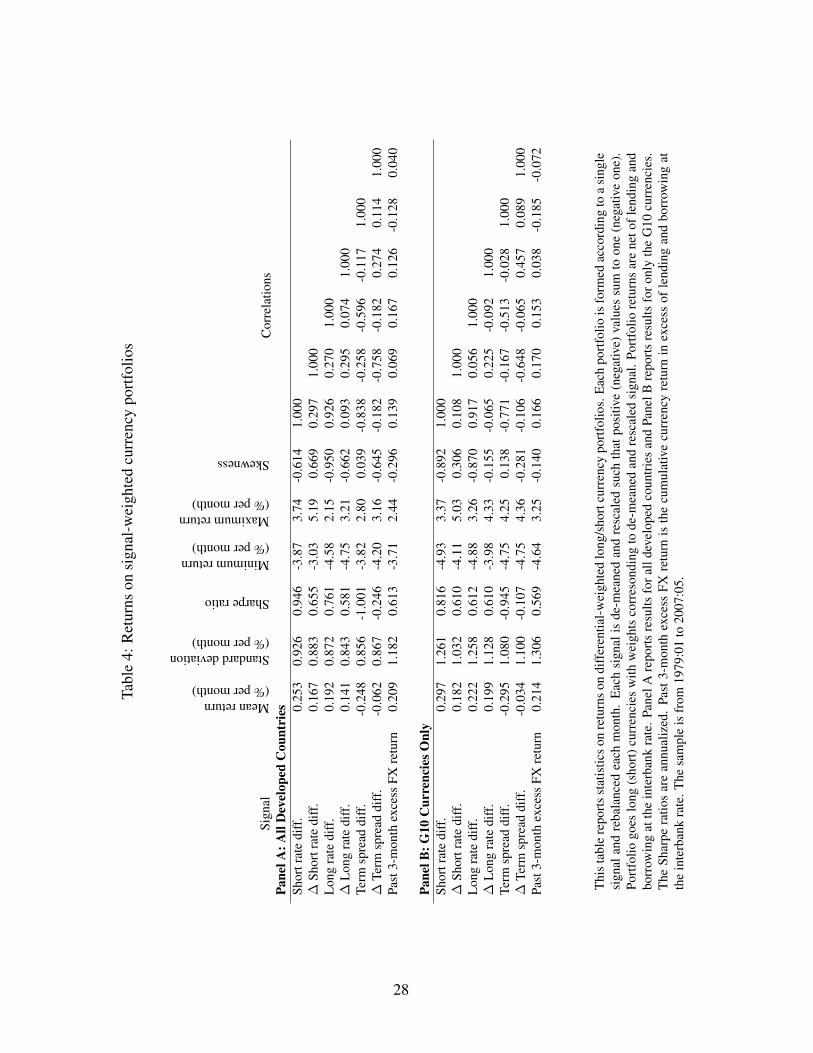
The returns on these signal-weighted currency returns are presented in Table 4. Overall,
we find similar results as equal-weighted currency returns, but with some differences. We find
that the signal-weighted carry trade still has an impressively high Sharpe ratio, but is negatively
skewed. The changes in the short rate produces a portfolio with high Sharpe ratio and more
positively skewed portfolios than before. The correlation between the two remain low. Currency
portfolio based on long rate differentials still looks similar to the carry trade. However, changes
in the long rate differentials appears to be predictive and contains information not already found
in the short rate.
The returns on currency portfolios based on term spread and currency momentum are similar
when signal-weighted as well. The term spread differentials still produce the single portfolio
with the greatest Sharpe ratio, and has little skewness. Expressing yield curve information this
way, changes in the term spread produces a portfolio with only a very modest Sharpe ratio.
Currency momentum portfolios also continue to produce high Sharpe ratios, but its returns have
low correlations with returns of portfolios formed using yield curve information.
These signal-weighted portfolios alleviate concerns that neither the truncation of outliers or
17
discreteness of the cut-off point somehow affect our currency portfolio results. These portfolios
are also much closer to running regressions and make comparisons easier. We turn to our
regression framework in the next section.
6 Predictive Regression Framework
6.1 Cross-Sectional Regression Specification
In our cross-sectional regression specification, we maintain comparability with our portfolio
results. The dependent variable is future excess currency returns, but we vary the horizon from
1-month to 12-month. Longer horizon returns are cumulated, but we express the returns in
monthly figures to make comparison easier. Our basic specification is a pooled-panel monthly
frequency regression with month fixed-effects. The month fixed-effects absorb any average
time-series variations in excess currency returns. This removes the effect of US dollar move-
ment across time relative to other currencies. All of our regressions use standard errors that
are heteroskedasticity-robust and double-clustered by month and currency. Hence, our stan-
dard errors account for variability in currency volatility over time, account for correlations of
currencies at any point in time, and account for auto-correlations of currencies.
There are also time-variations in the distribution of our signals. For example, we witnessed
in Figure 2 that there are periods of high variability and low variability in short rate differentials.
There are also outliers in data. To account for these features, we transform each of our inde-
pendent variables each month. We primarily consider regressors that have been transformed to
a uniform distribution ranging between 0 and 1, according to the rank of the variable. As an
example, if there are 10 currencies, the regressors are transformed to values of 0.05, 0.15, 0.25,
... and 0.95 according to the rank of the variable each month. For robustness checks, we also
standardize our regressors to be zero mean and unit variance within each month. For the most
part, we consider a sample consisting of all developed countries, but also consider a sample
consisting of only G10 currencies. We transform our regressors separately for each sample.
6.2 Regression Results
We begin by examining the univariate regressions in Table 5. Going across the columns, we
vary the holding period horizon of currencies as our dependent variable. Panel A predicts future
currency returns using short rate differentials and is comparable to the carry trade. Similar to the
18
carry trade, we find a positive relation between short rates and future excess currency returns.
As we vary the horizon, we find that predictability remains. Notice that even though the point
estimate falls with horizon, the t-statistics and remain largely unchanged.
We examine other yield curve predictors in Panels B through Panel D. We see the similar set
of results based on regressions as we did based on portfolios. Whether we use the changes in the
short rate differentials, the long rate differentials or the changes in the long rate differentials, we
continue to find positive relation between them and future currency returns. We also find that the
predictive ability is maintained but erodes as we increase the horizon. At some longer horizons,
we find that the predictability becomes weaker for the change in the long rate differentials. This
is in contrast to the negative correlations of the mean we observed in Panel A of Table 1. These
results suggest that there is a more complex time-series relation at play between the relation
between changes in interest rate and future exchange rates. The longer-horizon predictability
also suggests that portfolio strategies based on changes in interest rates can be constructed in a
way that portfolio turnover is not as high.
Given the regression framework, we can easily see if these yield curve predictors have in-
formation that are independent from one another through the use of multivariate regressions.
We compare levels and changes on short rate differentials in Panel A of Table 6, and compare
the levels and changes of long rate differentials in Panel B of Table 6. In both cases, the lev-
els of interest rate differentials and the changes in the interest rate differentials continue to be
significant as they did by themselves. This is similar to the low correlations we saw in the
portfolio framework. Hence we can conclude that both levels and changes of interest rates have
predictive information for future currency returns.
We compare the predictive ability of all four yield curve variables in Panel C of Table 6.
These are multivariate regressions where all four variables are used simultaneously. This speci-
fication allows us to understand how many different mechanisms are present. We find that when
all four variables are used, the long rate differentials no longer enter significantly, let alone pos-
itively. This is consistent with all the correlations we have seen thus far. It appears that long
rate differentials and short rate differentials, capture roughly the same set of information. How-
ever, we find that the changes in long rate differential is not driven out and remains positive and
statistically significant. Overall, it appears that there is more predictive information in the yield
curve than just levels and changes, and the shape of the yield is also important.
19
6.3 Robustness of Regressions Results
We address some robustness of our regression results in Table 7. We only consider the one-
month ahead excess currency return in our robustness, but vary the sample and the transfor-
mation of our regressors. The first column repeats the information in Table 6 for comparative
purposes. In the second column, we repeat the exercise but using only the G10 currencies.
We find that the point estimate on short rate differential is higher but with higher standard er-
rors, consistent with an observation on Table 3. Otherwise, we also find that the coefficient on
changes in short rate in Panel C is weaker and only significant at the 10% level. In the third and
fourth columns, we consider standardizing our regressors instead of putting them on a uniform
distribution. We find that all of our results remain qualitatively unchanged. If anything, the co-
efficient on changes in short rate is more robust to the sample, though it is now only significant
at the 5% level.
As an additional robustness, we consider using the information in the yield curve differently.
Rather than looking at the short rate differentials and the long rate differentials, we consider
using the short rate differentials and the term spread differentials. Similarly, we consider the
change in the term spread instead of the changes in the long rate differentials. Table 8 report
the regression results using the term spread differentials. These results are comparable to the
results in Panel C of Table 6 and Panel C of 7. Interestingly, rather than the change in the long
rate entering consistently significantly, we find that it’s the level of the term spread that enters
consistently. The changes in the term spreads also enter significantly at times. However, this
specification is not preferable because the term spread is strongly negative correlated with the
short rate, by construction. We see that this near collinearity drives out the predictability using
the short rate when only the G10 currencies are considered.
7 Conclusion
We find that there is significant information in foreign countries’ yield curves that is useful
for predicting foreign exchange returns in the cross-section. This predictability information
goes well beyond the uncovered interest parity and the violations of it, and it goes beyond
the well-known carry trade. We document that both the levels of interest rates as well as the
changes in interest rates have the ability to forecast future currency returns in the cross-section
of currencies. Moreover additional predictability information can be found by comparing the
movements in the short rates relative to that of the long rates. In particular, we find that in
20
addition to the levels and the changes of the short rate, the changes in the long rate or the levels
of the yield curve provides added predictability.
Overall, our empirical results are consistent with our motivating framework that risk fac-
tors the affect the yield curve should also affect the foreign exchange rates. Our findings fit
nicely with the term structure literature that document there appears to be multiple factors that
the term structure of interest rates. However, our paper only suggests that our findings can be
explained in a no-arbitrage model. We cannot rule out that profitability of the currency portfo-
lios we investigate is not due to mispricing rather than due to risk-exposure. We leave further
understanding of the economics behind our empirical findings to future work.
21
References[1] Ahn, D. H., 2004, “Common Factors and Local Factors: Implications for Term Structures and Exchange
Rates,” Journal of Financial and Quantitative Analysis, 39, 69-102.
[2] Ang, A., and M. Piazzesi, 2003, “A No-Arbitrage Vector Autoregression of Term Structure Dynamics withMacroeconomic and Latent Variables,” Journal of Monetary Economics, 50, 745-787.
[3] Backus, D. K., S. Foresi, and C. I. Telmer, 2001, “Affine Term Structure Models and the Forward PremiumAnomaly,” Journal of Finance, 56, 279-304.
[4] Balduzzi, P., S. R. Das, and S. Foresi, 1998, “The Central Tendency: A Second Factor in Bond Yields,”Review of Economics and Statistics, 80, 62-72.
[5] Balduzzi, P., S. R. Das, S. Foresi, and R. K. Sundaram, 1996, “A Simple Approach to Three-Factor AffineTerm Structure Models,” Journal of Fixed Income, 6, 43-53.
[6] Bansal, R., 1997, “An Exploration of the Forward Premium Puzzle in Currency Markets,” Review of Finan-cial Studies, 10, 369-403.
[7] Bekaert, G., 1996, “The Time Variation of Risk and Return in Foreign Exchange Markets,” Review of Fi-nancial Studies, 10, 369-403.
[8] Boudoukh, J., M. Richardson, and R. F. Whitelaw, 2006, “The Information in Long-Maturity Forward Rates:Implications for Exchange Rates and the Forward Premium Anomaly,” working paper, NYU.
[9] Brandt, M. W., and Q. Kang, 2004, “On the Relationship Between the Conditional Mean and Volatility ofStock Returns: A Latent VAR Approach,” Journal of Financial Economics, 72, 217-257.
[10] Brandt, M. W., and P. Santa-Clara, 2002, “Simulated Likelihood Estimation of Diffusions with an Applica-tion to Exchange Rate Dynamics in Incomplete Markets,” Journal of Financial Economics 63, 161-210.
[11] Brennan, M. J., and E. S. Schwartz, 1979, “A Continuous Time Approach to the Pricing of Bonds,” Journalof Banking and Finance, 3, 133-155.
[12] Brennan, M. J., A. W. Wang, and Y. Xia, 2004, “Estimation and Test of a Simple Model of IntertemporalAsset Pricing,” Journal of Finance, 59, 1743-1775.
[13] Brunnermeir, M. K., S. Nagel, and L. H. Pedersen, 2009, “Carry Trades and Currency Crashes,” in Ace-moglu, D., K. Rogoff, and M. Woodford, NBER Macroeconomics Annual, pp313-359, University ofChicago Press, Chicago IL.
[14] Burnside, C., M. S. Eichenbaum, I. Kleshchelski, and S. Rebelo, 2006, “The Returns to Currency Specula-tion,” NBER working paper 12489.
[15] Burnside, C., M. S. Eichenbaum, and S. Rebelo, 2007, “Understanding the Forward Premium Puzzle: AMicrostructure Approach,” NBER working paper 13278.
[16] Chen, Y. C., and K. P. Tsang, 2009, “What does the Yield Curve Tell Us about Exchange Rate Predictability,”working paper, University of Washington.
[17] Chinn, M. D., 2006, “The (Partial) Rehabilitation of Interest Rate Parity in the Floating Rate Era: LongerHorizons, Alternative Expectations, and Emerging Markets,” Journal of International Money and Finance,25, 7-21.
[18] Cox, J. C., J. E. Ingersoll, and S. A. Ross, 1985, “A Theory of the Term Structure of Interest Rates,”Econometrica, 53, 769-799.
22
[19] Dai, Q., and K. J. Singleton, 2000, “Specificaiton Analysis of Affine Term Structure Models,” Journal ofFinance, 55, 1943-1978.
[20] Dong, S., 2006, “Macro Variables Do Drive Exchange Rate Movements: Evidence from a No-ArbitrageModel,” working paper, Columbia University.
[21] Engel, C., 1996, “The Forward Discount Anomaly and the Risk Premium: A Survey of Recent Evidence,”Journal of Empirical Finance, 3, 123-92.
[22] Engel, C., and K. D. West, 2005, “Exchange Rates and Fundamentals,” Journal of Political Economy, 113,485-517.
[23] Engel, C., N. C. Mark, and K. D. West, 2007, “Exchange Rate Models are Not as Bad as You Think,” inAcemoglu, D., K. Rogoff, and M. Woodford, NBER Macroeconomics Annual, pp381-441, University ofChicago Press, Chicago IL.
[24] Fama, E., 1984, “Forward and Spot Exchange Rates,” Journal of Monetary Economics, 14, 319-338.
[25] Gourinchas, P. O., and A. Tornell, 2004, “Exchange Rate Puzzles and Distorted Beliefs,” Journal of Inter-national Economics, 64, 303-333.
[26] Graveline, J. J., 2006, “Exchange Rate Volatility and the Forward Premium Anomaly,” working paper, MIT.
[27] Hodrick, R. J., 1998, The Empirical Evidence on the Efficiency of Forward and Futures Foreign ExchangeMarkets, Harwood Academic, New York NY.
[28] Hodrick. R. J., and M. Vassalou, 2002, “Do we Need Multi-Country Models to Explain Exchange Rate andInterest Rate and Bond Return Dynamics?” Journal of Economic Dynamics and Control, 26, 1275-1299.
[29] Ilmanen, A., and R. Sayood, 1998, “Currency Allocaiton and Timing Based on Predictive Indicators,” Sa-lomon Smith Barney research report.
[30] Ilmanen, A., and R. Sayood, 2002, “Quantitative Forecasting Models and Active Diversification for Interna-tional Bonds,” Journal of Fixed Income, December, 40-51.
[31] Jurek, J. W., 2008, “Crash-Neutral Currency Carry Trades,” working paper, Princeton University.
[32] Kozicki, S., and P. A. Tinsley, 2001, “Shifting Endpoints in the Term Structure of Interest Rates,” Journal ofMonetary Economics, 47, 613-652.
[33] Lettau, M., and J. Wachter, 2009, “The Term Structures of Equity and Interest Rates,” working paper, UCBerkeley.
[34] Lewis, K. K., 1995, “Puzzles in International Financial Markets,” in Grossman, G. M. and Rogoff, K., eds,Handbook of International Economics, Elsevier, Amsterdam, pp1913-1972.
[35] Longstaff, F. A., and E. S. Schwartz, 1992, “Interest Rate Volatility and the Term Structure: A Two-FactorGeneral Equilibrium Model,” Journal of Finance, 47, 1259-1282.
[36] Lustig, H., N. Roussanov, and A. Verdelhan, 2008, “Common Risk Factors in Currency Markets,” NBERworking paper 14082.
[37] Molodtsova, T., and D. H. Papell, 2008, “Out-of-Sample Exchange Rate Predictability with Taylor RuleFundamentals,” working paper, Emory University.
[38] Piazzesi, 2003, “Affine Term Structure Models,” working paper, Stanford University.
23
[39] Sarno, L., 2005, “Towards a Solution to the Puzzles in Exchange Rate Economics: Where Do we Stand?”Canadian Journal of Economics, 38, 673-708.
[40] Schaefer, S. M., and E. S. Schwartz, 1979, “A Two-Factor Model of the Term Structure: An ApproximateAnalytical Solution,” Journal of Financial and Quantitative Analysis, 19, 413-424.
[41] Wang, J., and J. J. Wu, 2009, “The Taylor Rule and Interval Forecast for Exchange Rates,” working paper,Fed Board of Governors.
[42] Vasicek, O. A., 1977, “An Equilibrium Characterization of the Term Structure,” Journal of Financial Eco-nomics, 5, 177-188.
24
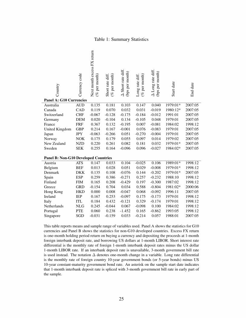
Table 1: Summary Statistics
Cou
ntry
Cur
renc
yco
de
Nex
tmon
thex
cess
FXre
turn
(%pe
rmon
th)
Shor
trat
edi
ff.
(%pe
rmon
th)
∆Sh
ortr
ate
diff
.(b
pspe
rmon
th)
Lon
gra
tedi
ff.
(%pe
rmon
th)
∆L
ong
rate
diff
.(b
pspe
rmon
th)
Star
tdat
e
End
date
Panel A: G10 CurrenciesAustralia AUD 0.135 0.181 0.103 0.147 0.040 1979:01* 2007:05Canada CAD 0.119 0.070 0.032 0.031 -0.019 1980:12* 2007:05Switzerland CHF -0.067 -0.128 -0.175 -0.184 -0.012 1991:01 2007:05Germany DEM 0.020 -0.104 0.134 -0.105 0.048 1979:01 2007:05France FRF 0.367 0.132 -0.195 0.007 -0.081 1984:02 1998:12United Kingdom GBP 0.214 0.167 -0.001 0.076 -0.083 1979:01 2007:05Japan JPY -0.063 -0.266 0.051 -0.270 -0.004 1979:01 2007:05Norway NOK 0.175 0.179 0.055 0.097 0.014 1979:02 2007:05New Zealand NZD 0.220 0.261 0.082 0.181 0.032 1979:01* 2007:05Sweden SEK 0.255 0.164 -0.096 0.096 -0.027 1984:02* 2007:05
Panel B: Non-G10 Developed CountriesAustria ATS 0.147 0.033 0.104 -0.025 0.106 1989:01* 1998:12Belgium BEF 0.013 0.028 0.051 0.029 -0.008 1979:01* 1998:12Denmark DKK 0.135 0.108 -0.076 0.144 -0.202 1979:01* 2007:05Spain ESP 0.259 0.386 -0.271 0.257 -0.232 1988:10 1998:12Finland FIM 0.165 0.208 -0.429 0.197 -0.300 1987:02 1998:12Greece GRD -0.154 0.704 0.034 0.588 -0.804 1981:02* 2000:06Hong Kong HKD 0.000 0.008 -0.047 0.068 -0.092 1996:11 2007:05Ireland IEP 0.167 0.253 -0.097 0.175 -0.173 1979:01 1998:12Italy ITL 0.184 0.432 -0.121 0.329 -0.174 1979:01 1998:12Netherlands NLG 0.245 -0.044 0.067 -0.098 0.100 1984:02 1998:12Portugal PTE 0.060 0.238 -1.452 0.165 -0.862 1993:05 1998:12Singapore SGD -0.031 -0.159 0.033 -0.214 0.057 1988:01 2007:05
This table reports means and sample range of variables used. Panel A shows the statistics for G10currencies and Panel B shows the statistics for non-G10 developed countries. Excess FX returnis one-month holding period return on buying a currency and depositing the proceeds at 1-monthforeign interbank deposit rate, and borrowing US dollars at 1-month LIBOR. Short interest ratedifferential is the monthly rate of foreign 1-month interbank deposit rates minus the US dollar1-month LIBOR rate. If an interbank deposit rate is unavailable, 3-month government bill rateis used instead. The notation ∆ denotes one-month change in a variable. Long rate differentialis the monthly rate of foreign country 10-year government bonds (or 5-year bonds) minus US10-year constant-maturity government bond rate. An asterisk on the sample start date indicatesthat 1-month interbank deposit rate is spliced with 3-month government bill rate in early part ofthe sample.
25
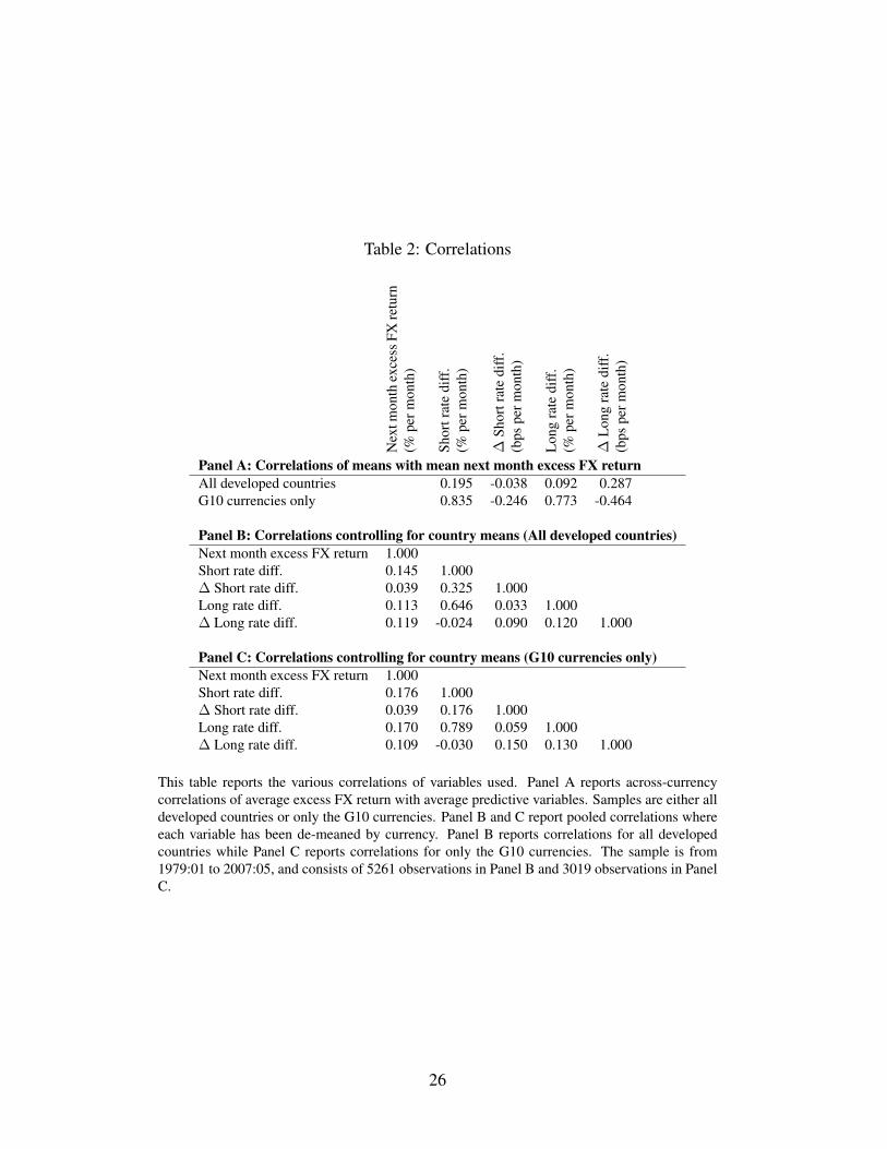
Table 2: Correlations
Nex
tmon
thex
cess
FXre
turn
(%pe
rmon
th)
Shor
trat
edi
ff.
(%pe
rmon
th)
∆Sh
ortr
ate
diff
.(b
pspe
rmon
th)
Lon
gra
tedi
ff.
(%pe
rmon
th)
∆L
ong
rate
diff
.(b
pspe
rmon
th)
Panel A: Correlations of means with mean next month excess FX returnAll developed countries 0.195 -0.038 0.092 0.287G10 currencies only 0.835 -0.246 0.773 -0.464
Panel B: Correlations controlling for country means (All developed countries)Next month excess FX return 1.000Short rate diff. 0.145 1.000∆ Short rate diff. 0.039 0.325 1.000Long rate diff. 0.113 0.646 0.033 1.000∆ Long rate diff. 0.119 -0.024 0.090 0.120 1.000
Panel C: Correlations controlling for country means (G10 currencies only)Next month excess FX return 1.000Short rate diff. 0.176 1.000∆ Short rate diff. 0.039 0.176 1.000Long rate diff. 0.170 0.789 0.059 1.000∆ Long rate diff. 0.109 -0.030 0.150 0.130 1.000
This table reports the various correlations of variables used. Panel A reports across-currencycorrelations of average excess FX return with average predictive variables. Samples are either alldeveloped countries or only the G10 currencies. Panel B and C report pooled correlations whereeach variable has been de-meaned by currency. Panel B reports correlations for all developedcountries while Panel C reports correlations for only the G10 currencies. The sample is from1979:01 to 2007:05, and consists of 5261 observations in Panel B and 3019 observations in PanelC.
26
Tabl
e3:
Ret
urns
oneq
ual-
wei
ghte
dcu
rren
cypo
rtfo
lios
Sign
al
Meanreturn(%permonth)
Standarddeviation(%permonth)
Sharperatio
Minimumreturn(%permonth)
Maximumreturn(%permonth)
Skewness
Cor
rela
tions
Pane
lA:A
llD
evel
oped
Cou
ntri
esSh
ortr
ate
diff
.0.
218
0.86
90.
870
-3.2
43.
27-0
.654
1.00
0∆
Shor
trat
edi
ff.
0.13
30.
673
0.68
3-2
.24
2.33
0.20
00.
139
1.00
0L
ong
rate
diff
.0.
151
0.81
00.
645
-4.0
02.
54-0
.968
0.87
20.
172
1.00
0∆
Lon
gra
tedi
ff.
0.10
70.
738
0.50
2-3
.02
2.29
-0.4
150.
022
0.24
2-0
.001
1.00
0Te
rmsp
read
diff
.-0
.222
0.78
7-0
.978
-2.9
92.
700.
073
-0.7
71-0
.110
-0.5
600.
000
1.00
0∆
Term
spre
addi
ff.
-0.0
610.
727
-0.2
91-2
.63
2.67
-0.3
28-0
.006
-0.5
27-0
.040
0.35
3-0
.017
1.00
0Pa
st3-
mon
thex
cess
FXre
turn
0.18
10.
961
0.65
2-3
.24
3.25
-0.0
390.
171
0.14
60.
191
0.02
7-0
.224
-0.1
42
Pane
lB:G
10C
urre
ncie
sOnl
ySh
ortr
ate
diff
.0.
275
1.18
90.
801
-4.6
03.
31-0
.830
1.00
0∆
Shor
trat
edi
ff.
0.17
10.
974
0.60
7-4
.31
3.40
-0.1
230.
097
1.00
0L
ong
rate
diff
.0.
222
1.19
70.
643
-4.6
04.
19-0
.690
0.85
90.
049
1.00
0∆
Lon
gra
tedi
ff.
0.17
41.
062
0.56
8-4
.17
4.59
-0.0
50-0
.148
0.29
6-0
.157
1.00
0Te
rmsp
read
diff
.-0
.270
1.08
5-0
.862
-5.1
03.
150.
032
-0.7
04-0
.190
-0.4
67-0
.004
1.00
0∆
Term
spre
addi
ff.
-0.0
311.
014
-0.1
08-4
.11
3.16
-0.2
08-0
.126
-0.4
40-0
.117
0.36
60.
064
1.00
0Pa
st3-
mon
thex
cess
FXre
turn
0.18
41.
241
0.51
3-4
.60
3.17
-0.0
820.
127
0.20
10.
195
0.04
7-0
.205
-0.0
52
Thi
sta
ble
repo
rts
stat
istic
son
retu
rns
oneq
ual-
wei
ghte
dlo
ng/s
hort
curr
ency
port
folio
s.E
ach
port
folio
isfo
rmed
acco
rdin
gto
asi
ngle
sign
alan
dre
bala
nced
each
mon
th.P
ortf
olio
goes
long
curr
enci
esw
ithth
ehi
ghes
tone
-thi
rdva
lue
ofa
sign
alan
dgo
essh
ortc
urre
ncie
sw
ithth
elo
wes
tone
-thi
rdva
lue
ofa
sign
al.
Port
folio
retu
rns
are
neto
fle
ndin
gan
dbo
rrow
ing
atth
ein
terb
ank
rate
.Pa
nelA
repo
rts
resu
ltsfo
ral
ldev
elop
edco
untr
ies
and
Pane
lBre
port
sre
sults
foro
nly
the
G10
curr
enci
es.T
heSh
arpe
ratio
sar
ean
nual
ized
.Pas
t3-m
onth
exce
ssFX
retu
rnis
the
cum
ulat
ive
curr
ency
retu
rnin
exce
ssof
lend
ing
and
borr
owin
gat
the
inte
rban
kra
te.T
hesa
mpl
eis
from
1979
:01
to20
07:0
5.
27
Tabl
e4:
Ret
urns
onsi
gnal
-wei
ghte
dcu
rren
cypo
rtfo
lios
Sign
al
Meanreturn(%permonth)
Standarddeviation(%permonth)
Sharperatio
Minimumreturn(%permonth)
Maximumreturn(%permonth)
Skewness
Cor
rela
tions
Pane
lA:A
llD
evel
oped
Cou
ntri
esSh
ortr
ate
diff
.0.
253
0.92
60.
946
-3.8
73.
74-0
.614
1.00
0∆
Shor
trat
edi
ff.
0.16
70.
883
0.65
5-3
.03
5.19
0.66
90.
297
1.00
0L
ong
rate
diff
.0.
192
0.87
20.
761
-4.5
82.
15-0
.950
0.92
60.
270
1.00
0∆
Lon
gra
tedi
ff.
0.14
10.
843
0.58
1-4
.75
3.21
-0.6
620.
093
0.29
50.
074
1.00
0Te
rmsp
read
diff
.-0
.248
0.85
6-1
.001
-3.8
22.
800.
039
-0.8
38-0
.258
-0.5
96-0
.117
1.00
0∆
Term
spre
addi
ff.
-0.0
620.
867
-0.2
46-4
.20
3.16
-0.6
45-0
.182
-0.7
58-0
.182
0.27
40.
114
1.00
0Pa
st3-
mon
thex
cess
FXre
turn
0.20
91.
182
0.61
3-3
.71
2.44
-0.2
960.
139
0.06
90.
167
0.12
6-0
.128
0.04
0
Pane
lB:G
10C
urre
ncie
sOnl
ySh
ortr
ate
diff
.0.
297
1.26
10.
816
-4.9
33.
37-0
.892
1.00
0∆
Shor
trat
edi
ff.
0.18
21.
032
0.61
0-4
.11
5.03
0.30
60.
108
1.00
0L
ong
rate
diff
.0.
222
1.25
80.
612
-4.8
83.
26-0
.870
0.91
70.
056
1.00
0∆
Lon
gra
tedi
ff.
0.19
91.
128
0.61
0-3
.98
4.33
-0.1
55-0
.065
0.22
5-0
.092
1.00
0Te
rmsp
read
diff
.-0
.295
1.08
0-0
.945
-4.7
54.
250.
138
-0.7
71-0
.167
-0.5
13-0
.028
1.00
0∆
Term
spre
addi
ff.
-0.0
341.
100
-0.1
07-4
.75
4.36
-0.2
81-0
.106
-0.6
48-0
.065
0.45
70.
089
1.00
0Pa
st3-
mon
thex
cess
FXre
turn
0.21
41.
306
0.56
9-4
.64
3.25
-0.1
400.
166
0.17
00.
153
0.03
8-0
.185
-0.0
72
Thi
sta
ble
repo
rts
stat
istic
son
retu
rns
ondi
ffer
entia
l-w
eigh
ted
long
/sho
rtcu
rren
cypo
rtfo
lios.
Eac
hpo
rtfo
liois
form
edac
cord
ing
toa
sing
lesi
gnal
and
reba
lanc
edea
chm
onth
.E
ach
sign
alis
de-m
eane
dan
dre
scal
edsu
chth
atpo
sitiv
e(n
egat
ive)
valu
essu
mto
one
(neg
ativ
eon
e).
Port
folio
goes
long
(sho
rt)c
urre
ncie
sw
ithw
eigh
tsco
rres
ondi
ngto
de-m
eane
dan
dre
scal
edsi
gnal
.Por
tfol
iore
turn
sar
ene
tofl
endi
ngan
dbo
rrow
ing
atth
ein
terb
ank
rate
.Pan
elA
repo
rts
resu
ltsfo
rall
deve
lope
dco
untr
ies
and
Pane
lBre
port
sre
sults
foro
nly
the
G10
curr
enci
es.
The
Shar
pera
tios
are
annu
aliz
ed.
Past
3-m
onth
exce
ssFX
retu
rnis
the
cum
ulat
ive
curr
ency
retu
rnin
exce
ssof
lend
ing
and
borr
owin
gat
the
inte
rban
kra
te.T
hesa
mpl
eis
from
1979
:01
to20
07:0
5.
28
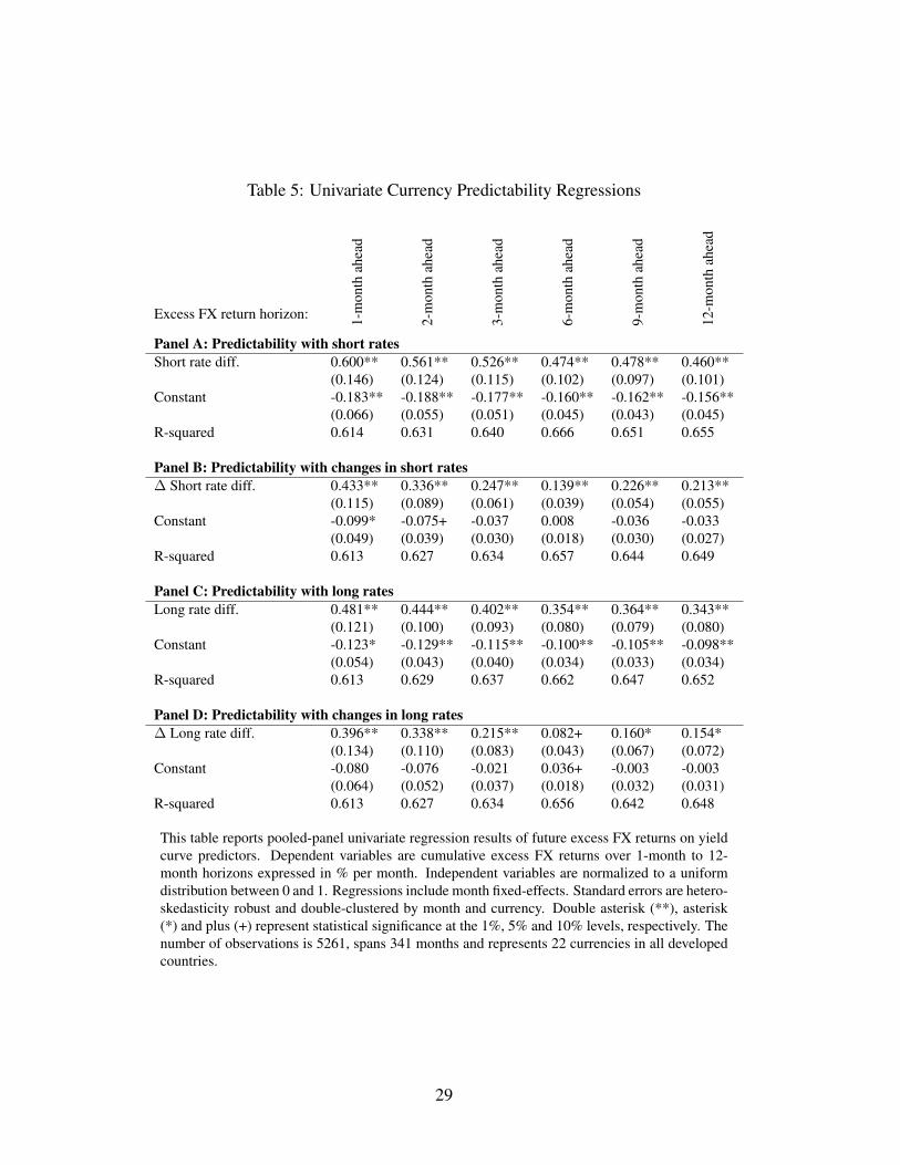
Table 5: Univariate Currency Predictability Regressions
Excess FX return horizon: 1-m
onth
ahea
d
2-m
onth
ahea
d
3-m
onth
ahea
d
6-m
onth
ahea
d
9-m
onth
ahea
d
12-m
onth
ahea
d
Panel A: Predictability with short ratesShort rate diff. 0.600** 0.561** 0.526** 0.474** 0.478** 0.460**
(0.146) (0.124) (0.115) (0.102) (0.097) (0.101)Constant -0.183** -0.188** -0.177** -0.160** -0.162** -0.156**
(0.066) (0.055) (0.051) (0.045) (0.043) (0.045)R-squared 0.614 0.631 0.640 0.666 0.651 0.655
Panel B: Predictability with changes in short rates∆ Short rate diff. 0.433** 0.336** 0.247** 0.139** 0.226** 0.213**
(0.115) (0.089) (0.061) (0.039) (0.054) (0.055)Constant -0.099* -0.075+ -0.037 0.008 -0.036 -0.033
(0.049) (0.039) (0.030) (0.018) (0.030) (0.027)R-squared 0.613 0.627 0.634 0.657 0.644 0.649
Panel C: Predictability with long ratesLong rate diff. 0.481** 0.444** 0.402** 0.354** 0.364** 0.343**
(0.121) (0.100) (0.093) (0.080) (0.079) (0.080)Constant -0.123* -0.129** -0.115** -0.100** -0.105** -0.098**
(0.054) (0.043) (0.040) (0.034) (0.033) (0.034)R-squared 0.613 0.629 0.637 0.662 0.647 0.652
Panel D: Predictability with changes in long rates∆ Long rate diff. 0.396** 0.338** 0.215** 0.082+ 0.160* 0.154*
(0.134) (0.110) (0.083) (0.043) (0.067) (0.072)Constant -0.080 -0.076 -0.021 0.036+ -0.003 -0.003
(0.064) (0.052) (0.037) (0.018) (0.032) (0.031)R-squared 0.613 0.627 0.634 0.656 0.642 0.648
This table reports pooled-panel univariate regression results of future excess FX returns on yieldcurve predictors. Dependent variables are cumulative excess FX returns over 1-month to 12-month horizons expressed in % per month. Independent variables are normalized to a uniformdistribution between 0 and 1. Regressions include month fixed-effects. Standard errors are hetero-skedasticity robust and double-clustered by month and currency. Double asterisk (**), asterisk(*) and plus (+) represent statistical significance at the 1%, 5% and 10% levels, respectively. Thenumber of observations is 5261, spans 341 months and represents 22 currencies in all developedcountries.
29
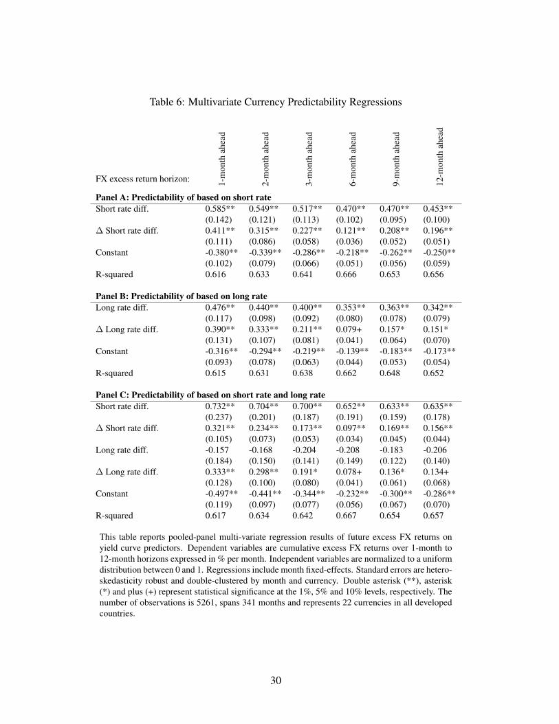
Table 6: Multivariate Currency Predictability Regressions
FX excess return horizon: 1-m
onth
ahea
d
2-m
onth
ahea
d
3-m
onth
ahea
d
6-m
onth
ahea
d
9-m
onth
ahea
d
12-m
onth
ahea
d
Panel A: Predictability of based on short rateShort rate diff. 0.585** 0.549** 0.517** 0.470** 0.470** 0.453**
(0.142) (0.121) (0.113) (0.102) (0.095) (0.100)∆ Short rate diff. 0.411** 0.315** 0.227** 0.121** 0.208** 0.196**
(0.111) (0.086) (0.058) (0.036) (0.052) (0.051)Constant -0.380** -0.339** -0.286** -0.218** -0.262** -0.250**
(0.102) (0.079) (0.066) (0.051) (0.056) (0.059)R-squared 0.616 0.633 0.641 0.666 0.653 0.656
Panel B: Predictability of based on long rateLong rate diff. 0.476** 0.440** 0.400** 0.353** 0.363** 0.342**
(0.117) (0.098) (0.092) (0.080) (0.078) (0.079)∆ Long rate diff. 0.390** 0.333** 0.211** 0.079+ 0.157* 0.151*
(0.131) (0.107) (0.081) (0.041) (0.064) (0.070)Constant -0.316** -0.294** -0.219** -0.139** -0.183** -0.173**
(0.093) (0.078) (0.063) (0.044) (0.053) (0.054)R-squared 0.615 0.631 0.638 0.662 0.648 0.652
Panel C: Predictability of based on short rate and long rateShort rate diff. 0.732** 0.704** 0.700** 0.652** 0.633** 0.635**
(0.237) (0.201) (0.187) (0.191) (0.159) (0.178)∆ Short rate diff. 0.321** 0.234** 0.173** 0.097** 0.169** 0.156**
(0.105) (0.073) (0.053) (0.034) (0.045) (0.044)Long rate diff. -0.157 -0.168 -0.204 -0.208 -0.183 -0.206
(0.184) (0.150) (0.141) (0.149) (0.122) (0.140)∆ Long rate diff. 0.333** 0.298** 0.191* 0.078+ 0.136* 0.134+
(0.128) (0.100) (0.080) (0.041) (0.061) (0.068)Constant -0.497** -0.441** -0.344** -0.232** -0.300** -0.286**
(0.119) (0.097) (0.077) (0.056) (0.067) (0.070)R-squared 0.617 0.634 0.642 0.667 0.654 0.657
This table reports pooled-panel multi-variate regression results of future excess FX returns onyield curve predictors. Dependent variables are cumulative excess FX returns over 1-month to12-month horizons expressed in % per month. Independent variables are normalized to a uniformdistribution between 0 and 1. Regressions include month fixed-effects. Standard errors are hetero-skedasticity robust and double-clustered by month and currency. Double asterisk (**), asterisk(*) and plus (+) represent statistical significance at the 1%, 5% and 10% levels, respectively. Thenumber of observations is 5261, spans 341 months and represents 22 currencies in all developedcountries.
30
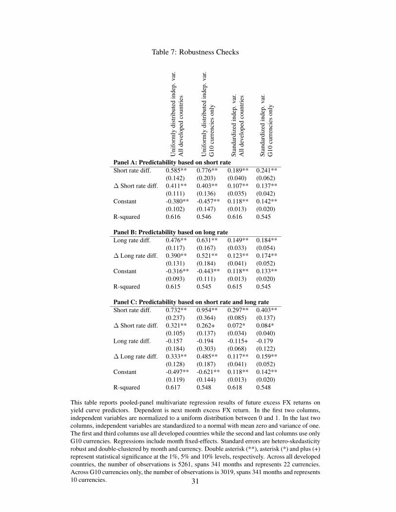
Table 7: Robustness Checks
Uni
form
lydi
stri
bute
din
dep.
var.
All
deve
lope
dco
untr
ies
Uni
form
lydi
stri
bute
din
dep.
var.
G10
curr
enci
eson
ly
Stan
dard
ized
inde
p.va
r.A
llde
velo
ped
coun
trie
s
Stan
dard
ized
inde
p.va
r.G
10cu
rren
cies
only
Panel A: Predictability based on short rateShort rate diff. 0.585** 0.776** 0.189** 0.241**
(0.142) (0.203) (0.040) (0.062)∆ Short rate diff. 0.411** 0.403** 0.107** 0.137**
(0.111) (0.136) (0.035) (0.042)Constant -0.380** -0.457** 0.118** 0.142**
(0.102) (0.147) (0.013) (0.020)R-squared 0.616 0.546 0.616 0.545
Panel B: Predictability based on long rateLong rate diff. 0.476** 0.631** 0.149** 0.184**
(0.117) (0.167) (0.033) (0.054)∆ Long rate diff. 0.390** 0.521** 0.123** 0.174**
(0.131) (0.184) (0.041) (0.052)Constant -0.316** -0.443** 0.118** 0.133**
(0.093) (0.111) (0.013) (0.020)R-squared 0.615 0.545 0.615 0.545
Panel C: Predictability based on short rate and long rateShort rate diff. 0.732** 0.954** 0.297** 0.403**
(0.237) (0.364) (0.085) (0.137)∆ Short rate diff. 0.321** 0.262+ 0.072* 0.084*
(0.105) (0.137) (0.034) (0.040)Long rate diff. -0.157 -0.194 -0.115+ -0.179
(0.184) (0.303) (0.068) (0.122)∆ Long rate diff. 0.333** 0.485** 0.117** 0.159**
(0.128) (0.187) (0.041) (0.052)Constant -0.497** -0.621** 0.118** 0.142**
(0.119) (0.144) (0.013) (0.020)R-squared 0.617 0.548 0.618 0.548
This table reports pooled-panel multivariate regression results of future excess FX returns onyield curve predictors. Dependent is next month excess FX return. In the first two columns,independent variables are normalized to a uniform distribution between 0 and 1. In the last twocolumns, independent variables are standardized to a normal with mean zero and variance of one.The first and third columns use all developed countries while the second and last columns use onlyG10 currencies. Regressions include month fixed-effects. Standard errors are hetero-skedasticityrobust and double-clustered by month and currency. Double asterisk (**), asterisk (*) and plus (+)represent statistical significance at the 1%, 5% and 10% levels, respectively. Across all developedcountries, the number of observations is 5261, spans 341 months and represents 22 currencies.Across G10 currencies only, the number of observations is 3019, spans 341 months and represents10 currencies. 31
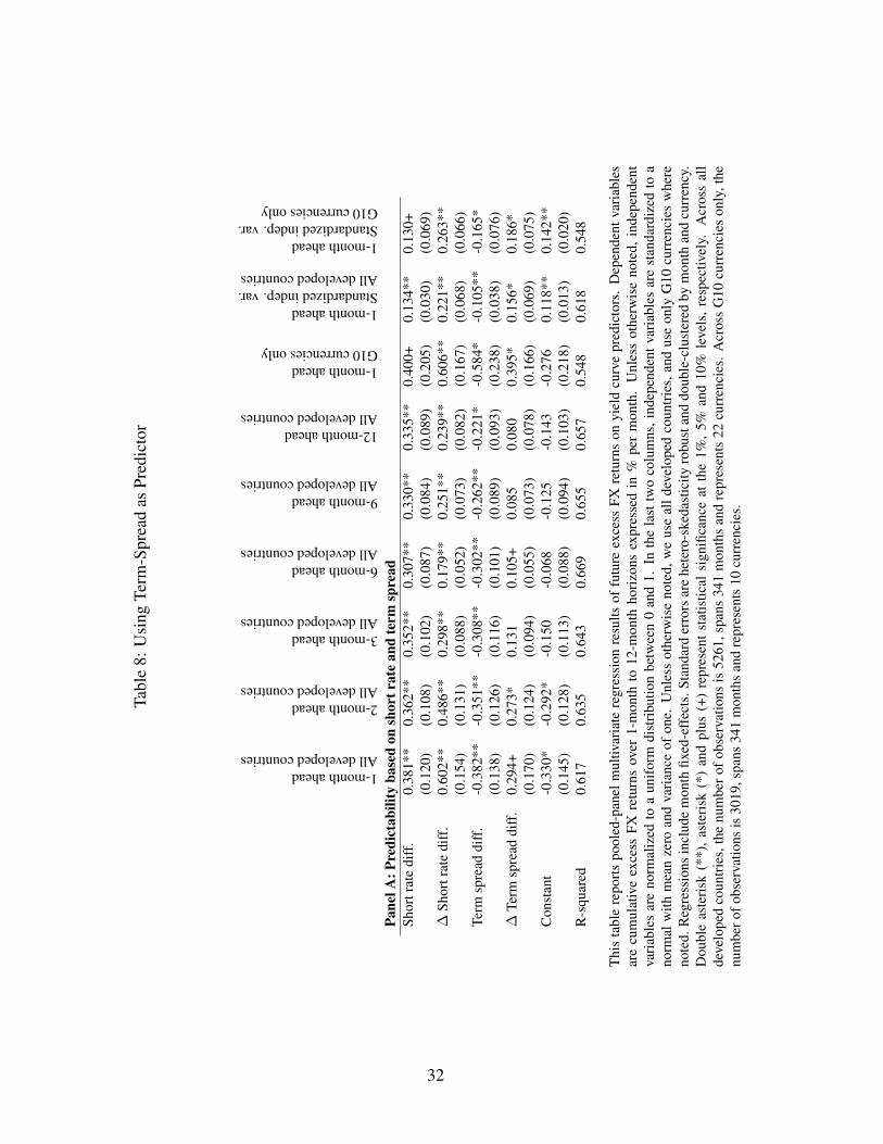
Tabl
e8:
Usi
ngTe
rm-S
prea
das
Pred
icto
r
1-monthaheadAlldevelopedcountries
2-monthaheadAlldevelopedcountries
3-monthaheadAlldevelopedcountries
6-monthaheadAlldevelopedcountries
9-monthaheadAlldevelopedcountries
12-monthaheadAlldevelopedcountries
1-monthaheadG10currenciesonly
1-monthaheadStandardizedindep.var.Alldevelopedcountries
1-monthaheadStandardizedindep.var.G10currenciesonly
Pane
lA:P
redi
ctab
ility
base
don
shor
trat
ean
dte
rmsp
read
Shor
trat
edi
ff.
0.38
1**
0.36
2**
0.35
2**
0.30
7**
0.33
0**
0.33
5**
0.40
0+0.
134*
*0.
130+
(0.1
20)
(0.1
08)
(0.1
02)
(0.0
87)
(0.0
84)
(0.0
89)
(0.2
05)
(0.0
30)
(0.0
69)
∆Sh
ortr
ate
diff
.0.
602*
*0.
486*
*0.
298*
*0.
179*
*0.
251*
*0.
239*
*0.
606*
*0.
221*
*0.
263*
*(0
.154
)(0
.131
)(0
.088
)(0
.052
)(0
.073
)(0
.082
)(0
.167
)(0
.068
)(0
.066
)Te
rmsp
read
diff
.-0
.382
**-0
.351
**-0
.308
**-0
.302
**-0
.262
**-0
.221
*-0
.584
*-0
.105
**-0
.165
*(0
.138
)(0
.126
)(0
.116
)(0
.101
)(0
.089
)(0
.093
)(0
.238
)(0
.038
)(0
.076
)∆
Term
spre
addi
ff.
0.29
4+0.
273*
0.13
10.
105+
0.08
50.
080
0.39
5*0.
156*
0.18
6*(0
.170
)(0
.124
)(0
.094
)(0
.055
)(0
.073
)(0
.078
)(0
.166
)(0
.069
)(0
.075
)C
onst
ant
-0.3
30*
-0.2
92*
-0.1
50-0
.068
-0.1
25-0
.143
-0.2
760.
118*
*0.
142*
*(0
.145
)(0
.128
)(0
.113
)(0
.088
)(0
.094
)(0
.103
)(0
.218
)(0
.013
)(0
.020
)R
-squ
ared
0.61
70.
635
0.64
30.
669
0.65
50.
657
0.54
80.
618
0.54
8
Thi
sta
ble
repo
rts
pool
ed-p
anel
mul
tivar
iate
regr
essi
onre
sults
offu
ture
exce
ssFX
retu
rns
onyi
eld
curv
epr
edic
tors
.D
epen
dent
vari
able
sar
ecu
mul
ativ
eex
cess
FXre
turn
sov
er1-
mon
thto
12-m
onth
hori
zons
expr
esse
din
%pe
rm
onth
.U
nles
sot
herw
ise
note
d,in
depe
nden
tva
riab
les
are
norm
aliz
edto
aun
ifor
mdi
stri
butio
nbe
twee
n0
and
1.In
the
last
two
colu
mns
,ind
epen
dent
vari
able
sar
est
anda
rdiz
edto
ano
rmal
with
mea
nze
roan
dva
rian
ceof
one.
Unl
ess
othe
rwis
eno
ted,
we
use
alld
evel
oped
coun
trie
s,an
dus
eon
lyG
10cu
rren
cies
whe
reno
ted.
Reg
ress
ions
incl
ude
mon
thfix
ed-e
ffec
ts.S
tand
ard
erro
rsar
ehe
tero
-ske
dast
icity
robu
stan
ddo
uble
-clu
ster
edby
mon
than
dcu
rren
cy.
Dou
ble
aste
risk
(**)
,as
teri
sk(*
)an
dpl
us(+
)re
pres
ent
stat
istic
alsi
gnifi
canc
eat
the
1%,
5%an
d10
%le
vels
,re
spec
tivel
y.A
cros
sal
lde
velo
ped
coun
trie
s,th
enu
mbe
rof
obse
rvat
ions
is52
61,s
pans
341
mon
ths
and
repr
esen
ts22
curr
enci
es.
Acr
oss
G10
curr
enci
eson
ly,t
henu
mbe
rofo
bser
vatio
nsis
3019
,spa
ns34
1m
onth
san
dre
pres
ents
10cu
rren
cies
.
32
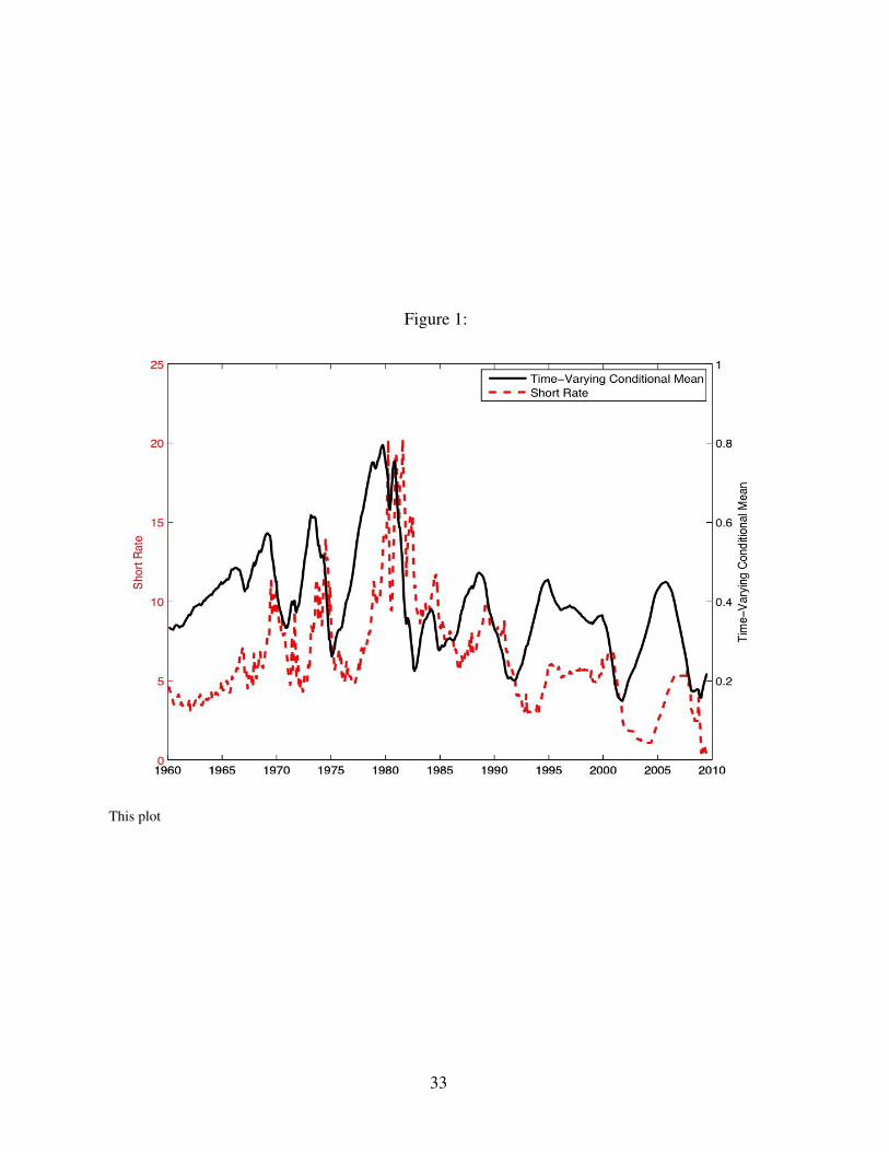
Figure 1:
This plot
33
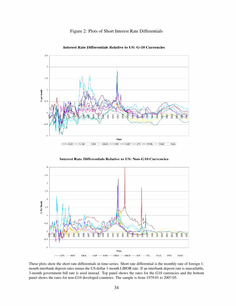
Figure 2: Plots of Short Interest Rate Differentials
These plots show the short rate differentials in time-series. Short rate differential is the monthly rate of foreign 1-month interbank deposit rates minus the US dollar 1-month LIBOR rate. If an interbank deposit rate is unavailable,3-month government bill rate is used instead. Top panel shows the rates for the G10 currencies and the bottompanel shows the rates for non-G10 developed countries. The sample is from 1979:01 to 2007:05.
34
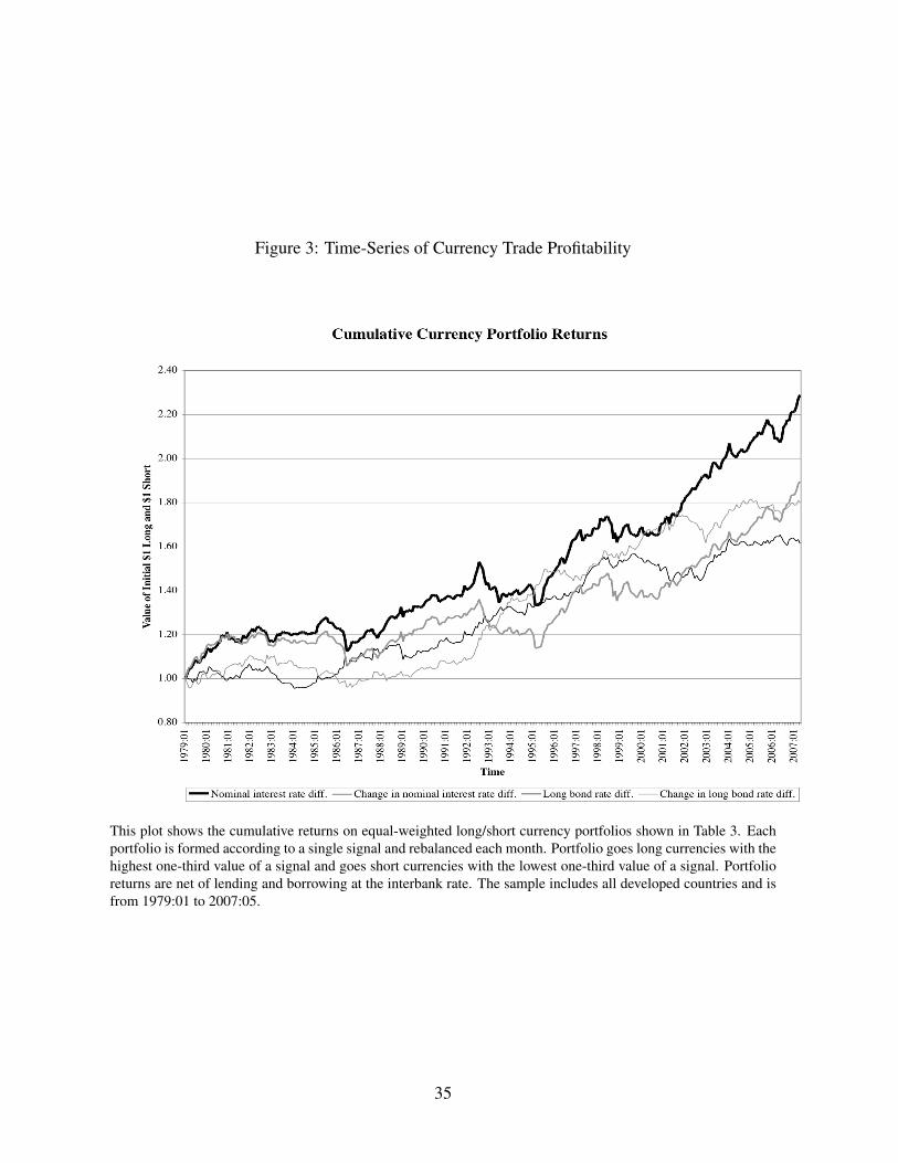
Figure 3: Time-Series of Currency Trade Profitability
This plot shows the cumulative returns on equal-weighted long/short currency portfolios shown in Table 3. Eachportfolio is formed according to a single signal and rebalanced each month. Portfolio goes long currencies with thehighest one-third value of a signal and goes short currencies with the lowest one-third value of a signal. Portfolioreturns are net of lending and borrowing at the interbank rate. The sample includes all developed countries and isfrom 1979:01 to 2007:05.
35
Recommended