11

Setembro de 2016 Working Paper

430

Determinants of the implied equity risk

premium in Brazil

Antonio Zoratto Sanvicente

Mauricio Rocha Carvalho

TEXTO PARA DISCUSSÃO 430 • SETEMBRO DE 2016 • 1

Os artigos dos Textos para Discussão da Escola de Economia de São Paulo da Fundação Getulio

Vargas são de inteira responsabilidade dos autores e não refletem necessariamente a opinião da

FGV-EESP. É permitida a reprodução total ou parcial dos artigos, desde que creditada a fonte.

Escola de Economia de São Paulo da Fundação Getulio Vargas FGV-EESP www.eesp.fgv.br

1

Determinants of the Implied Equity Risk Premium in Brazil

Antonio Zoratto Sanvicente, Escola de Economia de São Paulo, Fundação Getúlio

Vargas

Mauricio Rocha Carvalho, Insper, Instituto de Ensino e Pesquisa

April 2016

Abstract

This paper proposes and tests market determinants of the equity risk premium (ERP) in

Brazil. We use implied ERP, based on the Elton (1999) critique. The ultimate goal of

this exercise is to demonstrate that the calculation of implied, as opposed to historical

ERP makes sense, because it varies, in the expected direction, with changes in

fundamental market indicators. The ERP for Brazil is calculated as a mean of large

samples of individual stock prices in each month in the January, 1995 to September,

2015 period, using the “implied risk premium” approach. As determinants of changes in

the ERP we obtain, as significant, and in the expected direction: changes in the CDI

rate, in the country debt risk spread, in the US market liquidity premium and in the level

of the S&P500. The influence of the proposed determining factors is tested with the use

of time series regression analysis. The possibility of a change in that relationship with

the 2008 crisis was also tested, and the results indicate that the global financial crisis

had no significant impact on the nature of the relationship between the ERP and its

determining factors. For comparison purposes, we also consider the same variables as

determinants of the ERP calculated with average historical returns, as is common in

professional practice. First, the constructed series does not exhibit any relationship to

known market-events. Second, the variables found to be significantly associated with

historical ERP do not exhibit any intuitive relationship with compensation for market

risk.

Keywords: Equity risk premium; Discounted dividend model; Capital asset pricing

model.

2

1. Introduction

Any stock’s market risk premium, or “equity risk premium” (ERP), is given by the

difference between the expected return on the market portfolio and the rate of return on

the market’s risk-free asset. From one stock to another, the actual risk premium varies

with the particular stock’s beta, or sensitivity to returns on the market portfolio.

In many important applications, estimates of the expected return on the market portfolio

are made using averages of historical differences between returns on a stock market

index, such as the Standard & Poor’s 500 (S&P500) and a return on a riskless asset,

such as U.S. Treasury notes or bonds.

In Brazil, those important applications include: (a) the determination of discount rates in

order to value stocks of firms in acquisition and/or going private offers (OPAs); (b) the

setting of so-called “regulatory internal rates of return” for companies in regulated

sectors, such as electric power generation and distribution, highways, natural gas

distribution, among others. Internally, firms may need to calculate their cost of equity

capital as part of variable compensation schemes, or in the computation of their

weighted-average cost of capital when valuing new investment opportunities. This is

done because the Sharpe (1964), Lintner (1965), and Mossin (1966) version of the

capital asset pricing model (CAPM) is used in the construction of the relevant security

market line for estimating the appropriate opportunity cost of equity.

Two main issues stand out: (a) the already-mentioned use of historical return averages,

as opposed to current levels of the market portfolio’s expected return, in stark conflict

with the concept of an opportunity cost – for an individual or a firm that needs to make

an investment decision, the relevant cost should be that prevailing at the moment the

decision must be made, and not an average of what occurred in the past;1 (b) because

the available history for the Brazilian stock market is “short”, when compared to that of

the U.S. market, for example, one should use a U.S. market index as a proxy for the

market portfolio, and not Brazilian stock prices and returns, even when calculating an

equity risk premium for the Brazilian market.

In the present paper, we explain how to get around using historical averages as a basis

of estimating expected returns on the market portfolio, by describing a straightforward

procedure for obtaining the required expectation from current stock market prices. This

is known as an “implied” equity risk premium. We then present the resulting series for

the January 1995-September 2015 period, pointing out special situations, or “crises” in

which the expected market portfolio return spiked, as would be natural, as

compensation for sharp increases in the general level of risk perceived in the market.

1 In previous discussions, the authors have met with the contention that, if one uses historical averages of

very long periods of time, such as those available for the U.S. stock market, then the resulting estimate

would be “representative”. To this contention we simply offer the argument that, putting weak market

efficient considerations aside, this would be equivalent to saying that the distribution of rates of return is

stable throughout the historical period used, and that the “law of large numbers” applies, which simply

does not make sense in the case of financial asset prices and returns. It is much more plausible to admit

that the distribution of rates of return changes frequently and that one would do better by using an

approach that does not rely on assuming that the law of large numbers applies. Obviously, an historical

average does not change very frequently, but only with the slow addition of new observations as time

passes by.

3

We also test the significance and direction of the relationship between easily observed

market fundamentals and our estimate for the market portfolio’s return, and show that

the results are significant for certain fundamentals, and in the appropriate direction.

An alternative manner in which one can point out to problems with the use of historical

returns in the computation of equity risk premiums is to mention that the approach is

based on the assumption that information surprises involving business firms tend to

cancel each other over time, so that past behavior would become an unbiased estimator

of future behavior. Elton (1999) questions this fact, demonstrating that, in practice, this

has not occurred. Damodaran (2011) points out that this methodology puts us at a

crossroad: if we use a very long historical period in order to have a representative

sample (such as Ibbotson (2010), whose series starts in 1926), we would have to assume

that investors’ risk profiles and market fundamentals remained constant throughout that

period. On the other hand, if we reduce the period to the last 40 or 20 years, say, high

return volatility would produce unacceptably high standard errors. If that is the case for

a mature and liquid market such as the United States, that effect would certainly be

amplified in emerging markets such as Brazil. In addition, there is survivorship bias.

Market histories are studied with the use of stock indices, and clear evidence for this

bias in successful stock markets are presented and discussed in Brown et al. (1995).

The use of an implied premium is predicated on the idea that valuation and analysis

exercises must look forward in time and incorporate market expectations. Gebhardt et

al. (1999) use residual income models to estimate the implied cost of equity as the

internal rate of return produced by forecasted earnings, and implicit in current stock

prices. Claus and Thomas (1999) use the same idea in the aggregate. Damodaran (2011)

calculates the implied premium for the American and Brazilian markets.

The fact that implied risk premium and cost of equity calculations are gaining relevance

at the expense of the historical return approach is emphasized by Nekrasov and Ogneva

(2011), who enumerate some of the following applications: shedding light on the equity

premium puzzle (Claus and Thomas, 2001; Easton et al., 2002); the market’s perception

of equity risk (Gebhardt et al., 2001); risk associated with accounting restatements

(Hribar and Jenkins, 2004); legal institutions and regulatory regimes (Hail and Leuz,

2006); tests of the inter-temporal CAPM (Pastor et al., 2008), among others.

More recently, the cost of equity estimated with implied risk premium has been used as

dependent variable in corporate finance research, such as, for example, in Javakhadze et

al. (2016), in which the influence of managerial social capital, that is, the capital

constructed with the development of managers’ networks, benefits a firm through a

reduction in its cost of equity. The cost of equity was estimated with the use of the

dividend discount model, with data for 729 firms in all continents. Lima and Sanvicente

(2013) present evidence that better governance leads to reductions in the cost of equity

in the Brazilian market.

Hsing et al. (2011) applied the EGARCH model to the Brazilian stock index during

1997 until 2010 and find correlations with a few aggregate economic variables. The

market seems to be positively affected by industrial production, the ratio of M2 money

supply to GDP and the US stock market index. They also found a negative impact of the

lending rate, currency depreciation and domestic inflation.

4

Camacho and Lemme (2004) compared a set of 22 Brazilian companies with

investments abroad using two models: a Global CAPM and a Local CAPM to

investigate whether the cost of equity capital of Brazilian companies employed on

international investments should be greater than that used on national projects,

assuming an integrated market. They concluded that it is not correct to add any risk

premiums to the cost of domestic equity capital.

Ferreira (2011) observed the correlations between Brazilian macroeconomic variables

and the implied risk premium calculated using monthly data on stocks traded on the

Bovespa from January 2005 until December 2010. The results showed that the equity

risk premium demanded by investors is positively affected by the unexpected inflation

rate, the growth in money supply, the real interest rate, the output gap and it is

negatively affected by GDP growth.

A methodology for estimating the implied equity risk premium for the Brazilian market

is suggested in Minardi et alii. (2007). The proposal is to use business firm

fundamentals such as return on equity and payout ratio as inputs to the Gordon formula.

This is how the ERP for the Brazilian market is measured in the present paper.

The paper is organized as follows: section 2 reviews the literature, including previous

uses and tests of determinants of the ERP; section 3 describes the methodology for the

calculation of the ERP as implied by current stock prices; section 4 presents the

methodology for the analysis of risk premium determinants, including both the model

specification and the data used; the results are provided in section 5, and section 6

concludes and discusses both limitations and possible extensions.

2. Review of literature: implied equity risk premium and cost of equity

Claus and Thomas (1999) proposed a new approach to estimating the equity risk

premium for the U.S. market. This involved aggregating individual firm data and

determining the equity risk premium implied in current stock prices for a number of

firms, ranging from 1,559 in 1985 to 3,673 in 1998. Hence, they estimated a so-called

“implied market risk premium”. The implied equity risk premium was obtained as the

internal rate of return (k), in the following equation:

3 5 51 2 40 0 2 3 4 5 5

(1 '') (1)

(1 ) (1 ) (1 ) (1 ) (1 ) ( '')(1 )

ae ae ae gae ae aep bv

k k k k k k g k

Where, for the end of each year (t = 0,…,5):

p0 = current stock market price;

bv0 = book value of the firm’s equity, as disclosed in its financial statements;

aet = abnormal earnings, equal to reported earnings minus a charge for the cost of

equity, i.e., the product of beginning book value of equity and the implied rate of return;

this means that projected earnings for year t are given by et = bvt-1 + 0.5 x et-1, where the

et are analysts’ earnings forecasts; this is the so-called “clean surplus” approach, with

the added assumption of a common 50% payout ratio for all firms;

g’’ = the assumed constant growth rate in earnings in perpetuity, fixed at the real risk

free rate, that is, the then current 10-year T-bond rate minus 3% p. a. This growth rate is

applied to all earnings projected for t > 5, so that the last term in the equation above

5

represents what is usually referred to as the equity’s terminal value. In the calculation of

abnormal earnings for t = 1 to 5, the authors directly used analysts’ forecasts for years 1

and 2. For the remaining years (t = 3 to 5), they used g’, the implied growth rate in

analysts’ forecast for long-term earnings, that is, the forecasted 5-year growth rate.

This approach produced estimates of the equity risk premium of approximately 3% p.

a., with a low of 2.51% in 1997 and a high of 3.97% in 1995. This corresponds to

around half of the usually obtained premium on the basis of historical returns, that

apparently high level being the source of the so-called “equity premium puzzle” (Mehra

and Prescott, 1985).

In the calculation of the risk premium, the authors use the end-of-year 10-year Treasury

bond yield. They also discuss why this is an appropriate benchmark rate:

“There is some debate as to which maturity is appropriate when selecting the risk-free

rate. The risk premium literature has used both shorter (30-day or 1-year) and longer

(30-year) maturities for the risk-free rate. On the one hand, longer maturities exceed

the true risk-free rate because they incorporate the uncertainty associated with

intermediate variation in risk-free rates. On the other hand, short-term rates are likely

to be below the true risk-free rate, since some portion of the observed upward sloping

term structure could reflect increases in expected future short-term rates. Since the

flows (dividends or abnormal earnings) being discounted extend beyond one year, it

would not be appropriate to use the current short-term rate to discount flows that

have been forecast based on rising interest rates.” (Claus and Thomas, 1999, p. 16-

17)

In the appendix to their working paper, Claus and Thomas (1999) demonstrated that this

“accounting-based valuation model” is equivalent to the dividend growth approach used

in the present paper.

Claus and Thomas (1999) argue that, since earnings can be replaced by the

corresponding dividends in the equation above, one might think that there would be no

benefit in the use of earnings instead of dividends. Their contention, however, is: “the

main problem with using the dividend growth model resides in the arbitrary choice of

the assumed rate at which dividends grow in perpetuity” (Claus and Thomas, 1999, p.

9). This seems to be a strange argument, however, given their own need to propose a

value and a rationale for their g’’ rate.

Their working paper also makes an interesting and relevant comment on the relationship

between market efficiency and their approach to estimating an implied equity risk

premium (and any other approach based on current market prices, for that matter):

“Like other ex ante approaches, our approach assumes that the stock market

efficiently incorporates analyst forecasts into prices, and that analysts make unbiased

forecasts. There is however, a large body of research that has documented instances

of mispricing relating to information available in analyst forecasts, and also evidence

of various biases exhibited by analysts. Fortunately, the extent of mispricing

documented is relatively small. Also, the evidence on mispricing suggests that some

firms are underpriced and others are overpriced. Therefore, some of that mispricing

should cancel out at the market level, and be of less concern for our market-level

6

study”. (Claus and Thomas, 1999, pp. 10-11) [Emphasis added, since this applies fully

to our own approach in this paper.]

In several instances, Claus and Thomas (1999) refer to biases in analysts’ forecasts.

This is a problem avoided in our approach, as described in section 3, since the only

forecast we are required to make is the growth rate in perpetuity, from time t = 0 on,

given our assumed earnings and dividends growth process. In addition, the existing

coverage and availability of earnings forecasts by analysts for Brazilian firms is much

more limited:

“Turning to the issue of analysts making efficient forecasts, although some of the

biases exhibited by analysts would similarly cancel out in the aggregate, there is

evidence of a systematic optimism bias in analysts’ earnings forecasts.” (Claus and

Thomas, 1999, p. 11)

“Very few firms had negative values for 2-year-ahead forecasts, even though quite a

few firms reported losses in the current year.” (Claus and Thomas, 1999, p. 13)

“The contrast between our results and the traditional estimates of risk premium is

even starker in light of the well-known optimism in analyst forecasts.” (Claus and

Thomas, 1999, p. 19)

They point out that a downward adjustment in the implied risk premium would be

required to account for that optimism.

Finally, Claus and Thomas (1999) claim that their approach produces less variable

estimates than the dividend growth approach, and they believe this is a desirable

property, claiming that this is consistent with the view that the abnormal earnings

approach provides more reliable estimates. This is based on a comparison of the

resulting annual averages for k (the discount rate for projected abnormal earnings) and

for k* (the discount rate for projected dividends).

However, a counterargument would be as follows: since the resulting differences in

variability cannot be attributed to price variability, as the same prices are used in both

cases, it would be possible to attribute the lower variability of the earnings approach to

the management of disclosed earnings that they were not able to control for. In contrast,

dividend payments, even when based on managed earnings, are still dependent on a

decision, by a firm, that takes into account its capacity to make cash distributions to

investors, rendering dividends a more informative or even reliable indication of the

firm’s profitability prospects.

Gebhardt et al. (2001) use a similar approach to Claus and Thomas (1999): implied

costs of equity are estimated as the internal rate of return on projected earnings.

However, instead of making an attempt at estimating a market-wide average equity risk

premium, they test for several determinants of individual firm equity risk premiums.

Not surprisingly, proxies for risk (such as sector membership) and the magnitude of

growth opportunities (book-to-market ratio and forecasted long-term growth rate) prove

to be significant. Together with the dispersion in analyst earnings forecasts, they explain

approximately 60% of the variation in the cross section of implied costs of capital.

7

At the time, this article was part of an effort to answer the call by Elton (1999) for the

need for new approaches to risk premium estimation. Elton’s argument was as follows:

“Our approach is distinct from most of the prior empirical work on asset pricing in that

it does not rely on average realized returns.” (Elton, 1999, p. 2)

Operationally, they limit their earnings forecasting horizon to 3 years, instead of the 5-

year horizon in Claus and Thomas (1999), due to the availability of analyst forecasts,

thus circumventing the need for estimating the implied growth rate up to five years, as

described in Claus and Thomas (1999). They then make projections of annual earnings

up to 12 years. At t = 12 a terminal is value is computed. From t = 3 to t = 12, they

make the assumption that each firm’s return on equity (ROE) declines linearly to the

industry average. From t = 13 on, ROE is assumed to be equal to the cost of equity,

implying that there is no positive net present value contribution. This assumption is

used for all firms in their analysis, which range in number from 1,044 in 1979 to 1,333

in 1995. As in Claus and Thomas (1999), their proxy for the risk-free rate is also the 10-

year Treasury bond yield.

Because of these small differences in approach to Claus and Thomas (1999), they obtain

an average 2.7% equity risk premium for the entire period. However, their annual non-

weighted mean for the equity risk premium ranges from a high of 5.2% in 1979 to a low

of -0.2% in 1984. Note that these two years were not included in the Claus and Thomas

(1999) study which, as mentioned previously, covered the period from 1985 to 1998. In

their common coverage period (1985-1995), the two studies reported very similar

results, at least in terms of annual changes in the risk premium level. The overall period

averages in the common period are 3.44% p. a. (Claus and Thomas, 1999) and 3.17% p.

a. (Gebhardt et al., 2001). It should also be noted that the Claus and Thomas (1999)

“market-wide” premiums were computed as size-weighted averages of individual firm

estimates, not to mention the fact that the sample size in Claus and Thomas (1999) was

much larger, especially towards the end of the period they analyzed.

As a result of the dissatisfaction with the use of historical returns in tests of asset pricing

models, Elton’s American Finance Presidential Address (1999) makes a plea for the

adoption of new approaches.

Initially, he reminds us that “almost all of the testing” (Elton, 1999, p. 1199) involves

the use of realized returns as a proxy for expected returns, with the crucial reliance on

the belief that information surprises tend to cancel each other out over a study period, so

that realized returns would be an unbiased estimate of expected returns. As the reader

perfectly knows, asset pricing models do not purport to explain the setting of realized

returns, but of equilibrium expected returns.

Elton (1999) goes on to highlight long periods during which the average of stock market

returns was lower than the risk-free rate (from 1973 to 1984 in the US), as well as

periods in which the returns on risky longer-term bonds were also lower than the risk-

free rate (1927 to 1981). As he describes it, “… 11 and over 50 years is an awfully long

time for such a weak condition [that a risky asset should earn more than the risk-free

asset] not to be satisfied.” (Elton, 1999, p. 1199)

His main argument is that the plausible explanation of such apparently anomalous

results is that realized returns are poor measures of expected returns, since

8

“… information surprises highly influence a number of factors in our asset pricing

model. I believe that developing better measures of expected return and alternative

ways of testing asset pricing theories that do not require using realized returns

have a much higher payoff than any additional development of statistical tests that

continue to rely on realized returns as a proxy for expected returns.” (Elton, 1999,

p. 1199-1200) [Emphasis added]

A simple, but useful formalization of Elton’s (1999) point is as follows. Realized

returns can be decomposed into expected and unexpected returns:

1( ) (2)t t t tR E R e

where Rt is return in period t, Et-1(Rt) is expected return at t, conditional on the

information set available at time t - 1, and et is unexpected return.

In the discussion of stock market returns, the existing theories say that unexpected

return is caused by systematic factor shocks or unique firm-specific events. When one

uses realized returns as a proxy for expected returns, the hope is that unexpected returns

are independent. This would mean that, over long observation intervals, such as that

used as the basis for U.S. market premiums (usually, from 1926 on), those unexpected

returns tend to a mean of zero.

Elton’s argument, however, is that there tend to be information surprises which are very

large, or that a sequence of such surprises is correlated. This would make their

cumulative effect so large as to have a significant and permanent effect on the realized

mean, and would not disappear even as the observation interval becomes large.

The model he proposes is:

1( ) (3)t t t t tR E R I

where It is a significant information event. For Elton (1999), It is often equal to zero, but

occasionally it is a very large number (positive or negative). Hence, unexpected returns,

et = It + εt are in fact a mixture of two distributions, one with the usual properties (the εt,

independent and with zero mean), and a jump process for It.

Elton (1999) mentions the “McDonald’s effect” as an example of such a process. This

had to do with the fact that, in the 1950’s and 1960’s, there tended to be positive

earnings surprises for several years in succession. The series of high positive returns on

McDonald’s stock, when efficient frontiers were constructed on the basis of realized

returns tended to produce portfolios dominated by McDonald’s, and these “were simply

not credible”. (Elton, 1999, p. 1201)

Another example, and much closer to the present paper, is the effect of important

market-wide crises, such as that in the latter part of 2008. The effect of such a shock on

realized returns and their eventual use as the basis of estimates of risk premiums is

illustrated in Sanvicente (2012), with a focus on the use of such estimates by regulatory

agencies in Brazil.

9

3. Calculation of ERP implicit in current Brazilian market prices

The starting point in our ERP estimation methodology is the so-called Gordon model,

first proposed in Gordon (1959), which assumes that a stock’s dividends grow at the

constant rate g per period. The stock’s intrinsic value corresponds to the present value

of the stream of future dividends, discounted at ke, the firm’s opportunity cost of equity.

Given that dividends are assumed to grow at a constant rate, intrinsic value (V0) is the

present value of a perpetual stream of cash flows, and is obtained as follows:

10 (4)

e

DV

k g

where D1 is the dividend per share to be paid at the end of the first period (year).

Under the assumption that observed prices (P0) are equal to intrinsic values, except for a

random error, we can state that prices will contain information on the stock’s required

return, so that required return could be estimated as follows, for each individual stock:

1

0

(5)e

Dk g

P

We then construct the required return on the market portfolio, assumed to be equal to

the expected return, given the assumed equivalence of observed prices and intrinsic

values, by computing an average of the required returns for a representative sample of

individual stocks. In the tests run in this paper, we use a simple average, implying that

the proxy for the market portfolio is an equally-weighted portfolio of the stocks

included in the sample. Therefore, our assumed equality between observed prices and

intrinsic values is being proposed, not on a security-by-security basis, but on average for

the entire sample representing the market.

Prices P0 are directly observed. Given that 1 0(1 )D D g , and D0 (current dividend per

share) is also observed, the remaining task is to estimate the so-called “sustainable”

growth rate g (see Ross et al., 2012). Without changing either financing or dividend

policy, a firm can maintain the growth rate in both earnings and dividends through the

following relationship:

(6)g ROE b

where ROE = return on equity, or net income after taxes/net worth, and b = earnings

retention rate, or (1 – payout).

Since information on recent values of ROE, payout ratios and dividends per share are

available from financial statements, and prices are directly and continuously observed,

all the necessary data for estimating individual stock values for ke and calculating their

simple average are easily accessible.

In turn, the risk-free rate is obtained from current quotes of U.S. Treasury notes. Since

these instruments pay their income in U.S. dollars, we convert the local market data

using the Brazilian Real/U.S. dollar rate at each point in time.

10

The sample of individual stocks is processed as follows, for each month in the series:

a. Closing prices, 12-month net income, dividends and net worth per share are

collected. Obviously, stocks not traded at the end of any month are excluded from

the sample for that month. This still leaves a sample size, from January 1995 to

September 2015, of at least 90 firms, using only one class of stock for each firm in

the sample, which does not include financial institutions.

b. ROE and payout are computed as the ratios of net income/net worth, both on a per

share basis, and dividends per share/after-tax net income per share, respectively.

c. ROE and payout values are used for estimating g.

d. Equation (5) is then used in the estimation of ke, given the estimated values of D1 and

g, and the observed prices P0.

e. The simple average of the resulting individual values of ke is computed. This is the

estimate for the expected (required) return on the market.

f. The last step to calculate the ERP is to subtract, from the expected return on the

market (E(r)), the risk-free rate, obtained from current quotes of U.S. Treasury notes.

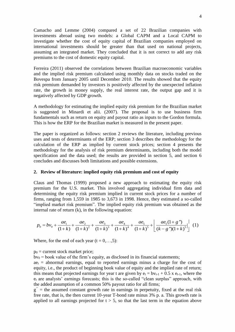
The procedure outlined above resulted in the following monthly series for the Brazilian

market’s ERP depicted in Figure 1.

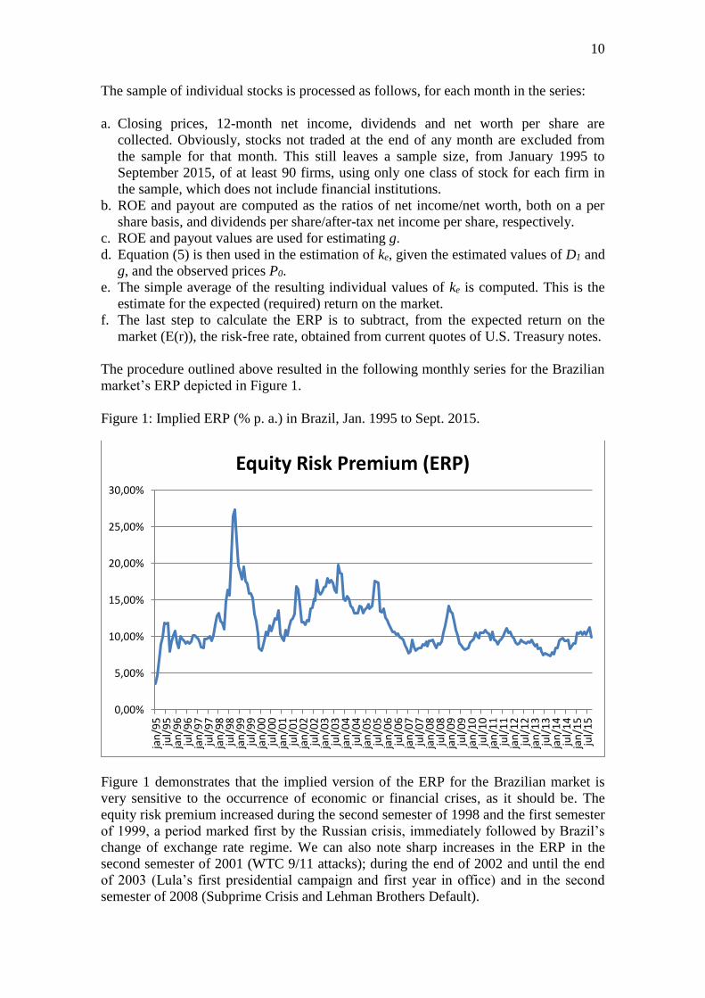
Figure 1: Implied ERP (% p. a.) in Brazil, Jan. 1995 to Sept. 2015.

Figure 1 demonstrates that the implied version of the ERP for the Brazilian market is

very sensitive to the occurrence of economic or financial crises, as it should be. The

equity risk premium increased during the second semester of 1998 and the first semester

of 1999, a period marked first by the Russian crisis, immediately followed by Brazil’s

change of exchange rate regime. We can also note sharp increases in the ERP in the

second semester of 2001 (WTC 9/11 attacks); during the end of 2002 and until the end

of 2003 (Lula’s first presidential campaign and first year in office) and in the second

semester of 2008 (Subprime Crisis and Lehman Brothers Default).

0,00%

5,00%

10,00%

15,00%

20,00%

25,00%

30,00%

jan/95

jul/95

jan/96

jul/96

jan/97

jul/97

jan/98

jul/98

jan/99

jul/99

jan/00

jul/00

jan/01

jul/01

jan/02

jul/02

jan/03

jul/03

jan/04

jul/04

jan/05

jul/05

jan/06

jul/06

jan/07

jul/07

jan/08

jul/08

jan/09

jul/09

jan/10

jul/10

jan/11

jul/11

jan/12

jul/12

jan/13

jul/13

jan/14

jul/14

jan/15

jul/15

Equity Risk Premium (ERP)

11

This sensitivity, in spite of being a drawback of the approach of estimating ERP with

current market prices, is a distinct advantage. It makes the ERP estimate responsive to

current market conditions, and hence a substantially more representative “price” of risk

than the estimates based on historical returns.

When a crisis ensues, there is an increase in the overall market aversion to risky assets;

investors demand higher returns in order to hold such assets. This is equivalent to seeing

investors discount future cash flows to those assets at higher rates, of which the ERP is

a common component. This process produces lower market valuations. In our approach,

this is represented by lower values for P0, higher values for ke, and hence, higher

estimates for the ERP. This sensitivity to changes in market conditions is a property that

the historical ERP approach does not possess. A dramatic example of the failure of the

historical ERP in this regard is provided in Sanvicente (2012), using data for the 2008

global financial crisis.

4. Methodology and data

We propose to explain the time series of implied ERP for Brazil using market variables,

or “fundamentals”. We believe they contain sufficient information about

macroeconomic data and expectations, with the advantage of being observed more

frequently and with no significant delays.

The basic specification proposes that the equity risk premium in Brazil is a function of

the exchange rate, the volatility of the Brazilian stock exchange, the volume traded in

the local stock market, the basic domestic interest rate, the U.S. liquidity premium,

Brazil’s country risk, the level of the stock exchange in the U.S., the price of gold, and

the domestic credit risk premium:

DERP = f(RPTAX, DVOLATIBOV, RVOLUMEIBOV, DCDI, DLIQPREM,

DRISKBR, RSP500, RGOLD, DCREDRISK)

Where:

DERP = first difference for the estimated value of the ERP

RPTAX = % change in the exchange rate of Reais to US$

DVOLATIBOV = first difference for historical Ibovespa volatility

RVOLUMEIBOV = % change in volume of trading in the Brazilian stock market

DCDI = first difference in domestic interest rates, proxied by the interbank market rate

DLIQPREM = first difference in the liquidity premium in international markets,

measured by the difference between US TBond (30-year) and TNote (10-year) yields

DRISKBR = first difference for the Brazil country risk spread, as measured by J. P.

Morgan’s EMBI+

RSP500 = rate of return on the S&P 500 index

RGOLD = % change in gold prices

DCREDRISK = first difference in a measure of credit default risk in Brazil, represented

by the spread between the average commercial bank lending rate to corporations and the

CDI (Brazilian Interbank Rate) on an annual basis.

12

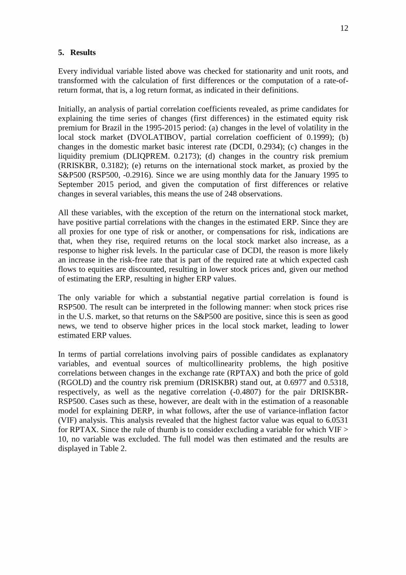
5. Results

Every individual variable listed above was checked for stationarity and unit roots, and

transformed with the calculation of first differences or the computation of a rate-of-

return format, that is, a log return format, as indicated in their definitions.

Initially, an analysis of partial correlation coefficients revealed, as prime candidates for

explaining the time series of changes (first differences) in the estimated equity risk

premium for Brazil in the 1995-2015 period: (a) changes in the level of volatility in the

local stock market (DVOLATIBOV, partial correlation coefficient of 0.1999); (b)

changes in the domestic market basic interest rate (DCDI, 0.2934); (c) changes in the

liquidity premium (DLIQPREM. 0.2173); (d) changes in the country risk premium

(RRISKBR, 0.3182); (e) returns on the international stock market, as proxied by the

S&P500 (RSP500, -0.2916). Since we are using monthly data for the January 1995 to

September 2015 period, and given the computation of first differences or relative

changes in several variables, this means the use of 248 observations.

All these variables, with the exception of the return on the international stock market,

have positive partial correlations with the changes in the estimated ERP. Since they are

all proxies for one type of risk or another, or compensations for risk, indications are

that, when they rise, required returns on the local stock market also increase, as a

response to higher risk levels. In the particular case of DCDI, the reason is more likely

an increase in the risk-free rate that is part of the required rate at which expected cash

flows to equities are discounted, resulting in lower stock prices and, given our method

of estimating the ERP, resulting in higher ERP values.

The only variable for which a substantial negative partial correlation is found is

RSP500. The result can be interpreted in the following manner: when stock prices rise

in the U.S. market, so that returns on the S&P500 are positive, since this is seen as good

news, we tend to observe higher prices in the local stock market, leading to lower

estimated ERP values.

In terms of partial correlations involving pairs of possible candidates as explanatory

variables, and eventual sources of multicollinearity problems, the high positive

correlations between changes in the exchange rate (RPTAX) and both the price of gold

(RGOLD) and the country risk premium (DRISKBR) stand out, at 0.6977 and 0.5318,

respectively, as well as the negative correlation (-0.4807) for the pair DRISKBR-

RSP500. Cases such as these, however, are dealt with in the estimation of a reasonable

model for explaining DERP, in what follows, after the use of variance-inflation factor

(VIF) analysis. This analysis revealed that the highest factor value was equal to 6.0531

for RPTAX. Since the rule of thumb is to consider excluding a variable for which VIF >

10, no variable was excluded. The full model was then estimated and the results are

displayed in Table 2.

13

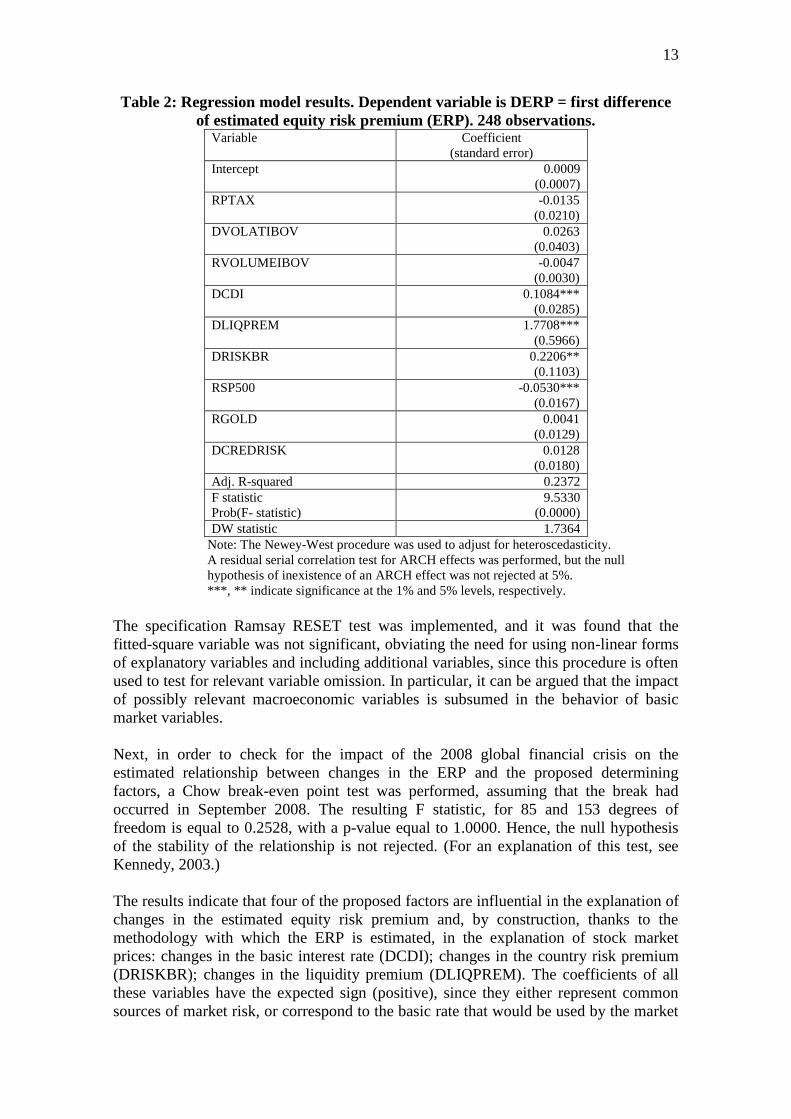
Table 2: Regression model results. Dependent variable is DERP = first difference

of estimated equity risk premium (ERP). 248 observations. Variable Coefficient

(standard error)

Intercept 0.0009

(0.0007)

RPTAX -0.0135

(0.0210)

DVOLATIBOV 0.0263

(0.0403)

RVOLUMEIBOV -0.0047

(0.0030)

DCDI 0.1084***

(0.0285)

DLIQPREM 1.7708***

(0.5966)

DRISKBR 0.2206**

(0.1103)

RSP500 -0.0530***

(0.0167)

RGOLD 0.0041

(0.0129)

DCREDRISK 0.0128

(0.0180)

Adj. R-squared 0.2372

F statistic

Prob(F- statistic)

9.5330

(0.0000)

DW statistic 1.7364

Note: The Newey-West procedure was used to adjust for heteroscedasticity.

A residual serial correlation test for ARCH effects was performed, but the null

hypothesis of inexistence of an ARCH effect was not rejected at 5%.

***, ** indicate significance at the 1% and 5% levels, respectively.

The specification Ramsay RESET test was implemented, and it was found that the

fitted-square variable was not significant, obviating the need for using non-linear forms

of explanatory variables and including additional variables, since this procedure is often

used to test for relevant variable omission. In particular, it can be argued that the impact

of possibly relevant macroeconomic variables is subsumed in the behavior of basic

market variables.

Next, in order to check for the impact of the 2008 global financial crisis on the

estimated relationship between changes in the ERP and the proposed determining

factors, a Chow break-even point test was performed, assuming that the break had

occurred in September 2008. The resulting F statistic, for 85 and 153 degrees of

freedom is equal to 0.2528, with a p-value equal to 1.0000. Hence, the null hypothesis

of the stability of the relationship is not rejected. (For an explanation of this test, see

Kennedy, 2003.)

The results indicate that four of the proposed factors are influential in the explanation of

changes in the estimated equity risk premium and, by construction, thanks to the

methodology with which the ERP is estimated, in the explanation of stock market

prices: changes in the basic interest rate (DCDI); changes in the country risk premium

(DRISKBR); changes in the liquidity premium (DLIQPREM). The coefficients of all

these variables have the expected sign (positive), since they either represent common

sources of market risk, or correspond to the basic rate that would be used by the market

14

to discount future cash flows to equities. The fourth empirically relevant variable

(RSP500) has a negative coefficient, and the manner in which it affects the value of

ERP in the Brazilian market was previously explained, corresponding to the fact that

prices in various national equity markets tend to co-vary in the same direction.

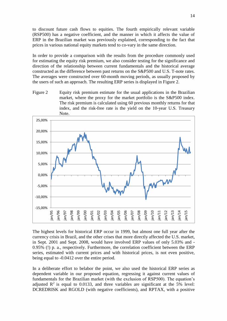
In order to provide a comparison with the results from the procedure commonly used

for estimating the equity risk premium, we also consider testing for the significance and

direction of the relationship between current fundamentals and the historical average

constructed as the difference between past returns on the S&P500 and U.S. T-note rates.

The averages were constructed over 60-month moving periods, as usually proposed by

the users of such an approach. The resulting ERP series is displayed in Figure 2.

Figure 2 Equity risk premium estimate for the usual applications in the Brazilian

market, where the proxy for the market portfolio is the S&P500 index.

The risk premium is calculated using 60 previous monthly returns for that

index, and the risk-free rate is the yield on the 10-year U.S. Treasury

Note.

The highest levels for historical ERP occur in 1999, but almost one full year after the

currency crisis in Brazil, and the other crises that more directly affected the U.S. market,

in Sept. 2001 and Sept. 2008, would have involved ERP values of only 5.03% and -

0.95% (!) p. a., respectively. Furthermore, the correlation coefficient between the ERP

series, estimated with current prices and with historical prices, is not even positive,

being equal to -0.0412 over the entire period.

In a deliberate effort to belabor the point, we also used the historical ERP series as

dependent variable in our proposed equation, regressing it against current values of

fundamentals for the Brazilian market (with the exclusion of RSP500). The equation’s

adjusted R2 is equal to 0.0133, and three variables are significant at the 5% level:

DCREDRISK and RGOLD (with negative coefficients), and RPTAX, with a positive

-15,00%

-10,00%

-5,00%

0,00%

5,00%

10,00%

15,00%

20,00%

25,00%

jan/95

jan/96

jan/97

jan/98

jan/99

jan/00

jan/01

jan/02

jan/03

jan/04

jan/05

jan/06

jan/07

jan/08

jan/09

jan/10

jan/11

jan/12

jan/13

jan/14

jan/15

15

coefficient. Intuitively, only the last result makes any sense – when the exchange rate

increases, so does the required return on the market portfolio.

6. Conclusion

This paper has examined potential market variables that can explain the movements in

the Brazilian market equity risk premium and, therefore, stock market prices. Monthly

samples from January 1995 until September 2015 were used in the construction of the

implied equity risk premium for the Brazilian market. The authors believe that using the

implied premium is a superior measure to the commonly used historic premiums

because the market should be affected by expected changes of returns, and not by

historic prices. Major findings are that the Brazilian market seems to be affected by two

local variables: 1) changes in local interest rates; 2) economic conditions that determine

the country risk premium. And it is also affected by two international market variables:

the U.S. liquidity premium and the level of U.S. equity prices. Other market variables

like the Real/U.S. dollar exchange rate, gold prices, stock market trading volume and

credit default risk were discarded as not being influential in the explanation of stock

market prices, possibly because the underlying economic factors are already represented

by the significant variables.

In an attempt to model the Brazilian market one should look at those four variables for

an explanation of our equity risk premium. Investors tend to demand higher rates of

return to invest in equities in Brazil than to invest in the U.S. The reasons for this

include the higher level of local interest rates and the higher sovereign risk. Those

explanations combined show why the Brazilian market is more complex and risky,

inducing rational investors to require higher expected rates of return.

Finally, the paper presented evidence of how inadequate the use of historically-based

premiums is for representing the market compensation for risk, leading to important

questions about the reasonableness of their use in so many practical applications.

7. References

Brown, S. J., Goetzmann, W. N. & Ross, S. A. (1995) Survival. The Journal of Finance,

50(3), 853-873.

Camacho, P. & Lemme, C. (2004). The cost of equity capital and the risk premium for

evaluating projects of Brazilian companies abroad: A study of the period from 1997 to

2002. Latin American Business Review, 5(3), 1-23.

Claus, J. & Thomas, J. (1999). The equity risk premium is much lower than you think it

is: empirical estimates from a new approach. Working paper. Columbia Business

School.

_____________. (2001). Equity premia as low as three percent? Evidence from

analysts’ earnings forecasts for domestic and international stock market. Journal of

Finance, 56, 1629-1666.

16

Damodaran, A. (2011) Equity Risk Premiums (ERP): Determinants, Estimation and

Implications – The 2011 Edition. Retrieved on 15 Dec. 2011, from

http://pages.stern.nyu.edu/~adamodar/.

Easton, P., Taylor, G., Shroff, P., & Sougiannis, T. (2002). Using forecasts of earnings

to simultaneous estimate growth and the rate of return on equity investments. Journal of

Accounting Research, 40, 657-676.

Elton, E. J. (1999). Expected return, realized return, and asset pricing tests. Journal of

Finance, 54(4)1199-1220.

Ferreira, L. F. (2011). Determinantes macroeconômicos do prêmio implícito por risco

de mercado no Brasil. Dissertação de Mestrado em Economia, Insper, São Paulo.

Available at <http://tede.insper.edu.br/tde_busca/processaPesquisa.php?nrPagina=6>.

Gebhardt, W. R., Lee, C. M. C. & Swaminathan, B. (2001). Toward an implied cost of

capital. Journal of Accounting Research, 39(1), 135-176.

Gordon, M. J. (1959). Dividends, earnings and stock prices. Review of Economics and

Statistics, 41(2), 99-105.

Hail, L., & Leuz, C. (2006). International differences in the cost of equity capital: Do

legal institutions and securities regulation matter? Journal of Accounting Research, 44,

485-532.

Hribar, P., & Jenkins, N. (2004). The effect of accounting restatements on earnings

revisions and the estimated cost of capital. Review of Accounting Studies, 9, 337-356.

Hsing, Yu, Phillips, A., & Phillips, C. (2011). Stock Prices and Aggregate Economic

Variables: The Case of Brazil. International Research Journal of Applied Finance,

II(5).

Ibbotson, R. (2010). Stocks, Bonds, Bills and Inflation Yearbook (SBBI) 2010 Edition,

Morningstar.

Javakhadze, D, Ferris, S. P., & French, D. W. (2016). Managerial Social Capital and

Financial Development: A Cross-Country Analysis. The Financial Review, v. 51(1), 37-

68.

Kennedy, P. (2003). A Guide to Econometrics, 5th. Ed. The MIT Press, Cambridge,

Massachusetts.

Lima, B. F., & Sanvicente, A. Z. (2013). The quality of corporate governance and cost

of equity in Brazil. Journal of Applied Corporate Finance, 25(1), 72-80.

Lintner, J. (1965). The valuation of risk assets and the selection of risky investments in

stock portfolios and capital budgets. Review of Economics and Statistics, 47(1), 13-37.

Mehra, R., & Prescott, E. C. (1985). The equity premium: a puzzle. Journal of

Monetary Economics, 15, 145-161.

17

Minardi, A. M. A. F., Sanvicente, A. Z., Montenegro, C. M. G., Donatelli, D. H., &

Bignotto, F. G. (2007). Estimando o custo de capital de companhias fechadas no Brasil

para uma melhor gestão estratégica de projetos. Insper Working Paper – WPE:

088/2007. Retrieved on February 15, 2012, from

http://www.insper.org.br/sites/default/files/2007_wpe088.pdf

Mossin, J. (1966). Equilibrium in a capital asset market. Econometrica, 34(4), 768-783.

Nekrasov, A., & Ogneva, M. (2011). Using earnings forecasts to simultaneously

estimate firm-specific cost of equity and long-term growth. Review of Accounting

Studies, 16, 414-457.

Pastor, L., Sinha, M., & Swaminathan, B. (2008). Estimating the intertemporal risk-

return tradeoff using the implied cost of capital. Journal of Finance, 63, 2859-2897.

Ross, S. A., Westerfield, R. J. & Jaffe, J. F. (2012). Corporate Finance, 11th ed. Boston,

MA, McGraw-Hill.

Sanvicente, A. Z. (2012). Problemas de estimação de custo de capital de empresas

concessionárias no Brasil: uma aplicação à regulamentação de concessões rodoviárias.

RAUSP, 47(1), 81-95.

Sharpe, W. F. (1964). Capital asset prices: A theory of market equilibrium. Journal of

Finance, 19(3), 425-442.