Embed Size (px)
Citation preview

Fraclet Predictor Overview
Presented byQuant Trade Technologies, Inc.

2
Contents
Introduction/Motivation
Survey and Lag Plots
Exact Problem Formulation
Proposed Method› Fractal Dimensions Background› Our method
Results
Conclusions

3
General Problem Definition
Given a time series {xt
}, predict its future course, that is, xt+1
, xt+2
, ...
Time
Value?

4
Motivation
• Financial data analysis
• Physiological data, elderly care
• Weather, environmental studies
Traditional fields
Sensor Networks (MEMS, “SmartDust”)• Long / “infinite”
series
• No human intervention “black box”

5
Traditional Forecasting Methods
ARIMA but linearity assumption
Neural Networks but large number of parameters and long training times
Hidden Markov Models O(N2) in number of nodes N; also fixing N is a problem
Lag Plots

6
Lag Plots
xt-1
xxtt
4-NNNew Point
Interpolate these…
To get the final prediction
Q0: Interpolation Method
Q1: Lag = ?
Q2: K = ?

7
Q0: Interpolation
Using SVD (state of the art)
Xt-1
xt

8
Why Lag Plots?› Based on the “Takens’ Theorem”
[Takens/1981]› which says that delay vectors can be
used for predictive purposes

9
Inside Theory
Example: Lotka-Volterra
equations
ΔH/Δt = rH
–
aH*P ΔP/Δt = bH*P –
mP
H is density of prey P is density of predators
Suppose only H(t) is observed. Internal state is (H,P).

10
Problem at hand
Given {x1 , x2 , …, xN }
Automatically set parameters
- L(opt) (from Q1) - k(opt) (from Q2)
in Linear time on N
to minimise Normalized Mean Squared Error (NMSE) of forecasting

11
Transform Data
0.1
0.2
0.3
0.4
0.5
0.6
0.7
0.8
0.9
1
0.1 0.2 0.3 0.4 0.5 0.6 0.7 0.8 0.9 1
x(t)
x(t-1)
Logistic Parabola
X(t-1)
X(t)
The Logistic Parabola xt
= axt-1
(1-xt-1
) + noise
time
x(t)
Intrinsic Dimensionality
≈
Degrees of Freedom
≈
Information about Xt
given Xt-1

CIKM 2002Your logo here 12
Cube the Data
0.1
0.2
0.3
0.4
0.5
0.6
0.7
0.8
0.9
1
0.1 0.2 0.3 0.4 0.5 0.6 0.7 0.8 0.9 1
x(t)
x(t-1)
Logistic Parabola
x(t-1)
x(t)
x(t-2)
x(t)
x(t)
x(t-2)
x(t-2) x(t-1)
x(t-1)
x(t-1)
x(t)

13
How Much Data is Enough?
To find L(opt):› Go further back in time (ie., consider Xt-2 , Xt-3
and so on)› Till there is no more information gained
about Xt

14
Fractal Dimensions
FD = intrinsic dimensionality
“Embedding”
dimensionality = 3
Intrinsic dimensionality = 1
15
Fractal Dimensions
FD = intrinsic dimensionality [Belussi/1995]
0
0.1
0.2
0.3
0.4
0.5
0.6
0.7
0.8
0.9
1
0 0.2 0.4 0.6 0.8 1 1.2 1.4 1.6 1.8 2
Y a
xis
X axis
Sierpinsky
7
8
9
10
11
12
13
14
15
16
-7 -6 -5 -4 -3 -2 -1 0 1 2
log
(# p
airs
with
in r
)
log(r)
FD plot
= 1.56
log(r)
log( # pairs)
Points to note:
• FD can be a non-integer
•
There are fast methods to compute it

16
Q1: Finding L(opt)
Use Fractal Dimensions to find the optimal lag length L(opt)
Lag (L)
Frac
tal D
imen
sion
epsilon
L(opt)
f
17
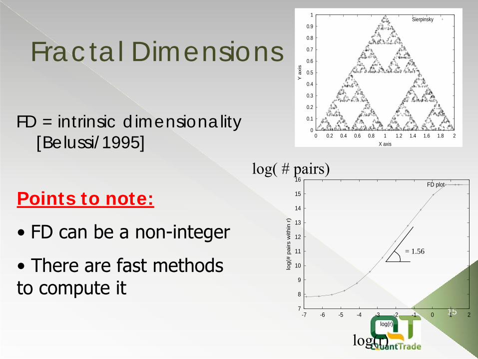
Q2: Finding k(opt)
To find k(opt)
• Conjecture: k(opt) ~ O(f)
We choose k(opt) =
2*f + 1

18
Logistic Parabola
0
0.5
1
1.5
2
2.5
3
1 2 3 4 5
Fra
ctal D
imensi
on
Lag
FD vs L
Our Choice
• FD vs
L plot flattens out
• L(opt) = 1
Timesteps
ValueLag
FD

19
Prediction
Timesteps
Value
Our Prediction from here

20
Logistic Parabola
Timesteps
Value
Comparison of prediction to correct values

21
Logistic Parabola
0
0.5
1
1.5
2
2.5
3
1 2 3 4 5
Fra
ctal
Dim
ensi
on
Lag
FD vs L
Our Choice
0
0.05
0.1
0.15
0.2
0.25
0.3
0.35
1 2 3 4 5 6
NM
SE
Lag
NMSE vs Lag
Our Choice
Our L(opt) = 1, which exactly minimizes NMSE
Lag
NM
SE
FD

22
Lorenz Attractor
0
0.5
1
1.5
2
2.5
3
1 2 3 4 5 6 7 8 9 10
Fra
ctal
Dim
ensi
on
Lag
FD vs L
Our Choice
• L(opt) = 5
Timesteps
Value
Lag
FD

23
Lorenz Attractor Prediction
Value
Timesteps
Our Prediction from here

24
Prediction Test
Timesteps
Value
Comparison of prediction to correct values
25
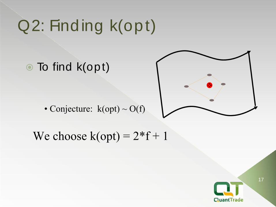
Optimal Prediction
0
0.5
1
1.5
2
2.5
3
1 2 3 4 5 6 7 8 9 10
Fra
ctal
Dim
ensi
on
Lag
FD vs L
Our Choice
L(opt) = 5
Also NMSE is optimal at Lag = 5
0
0.2
0.4
0.6
0.8
1
0 2 4 6 8 10 12
NM
SE
Lag
NMSE vs Lag
Our Choice
Lag
NM
SE
FD

26
Laser
0
0.5
1
1.5
2
2.5
3
3.5
1 2 3 4 5 6 7 8 9 10 11 12 13 14 15 16 17
Fra
ctal
Dim
ensi
on
Lag
FD vs L
Our Choice
• L(opt) = 7
Timesteps
Value
Lag
FD
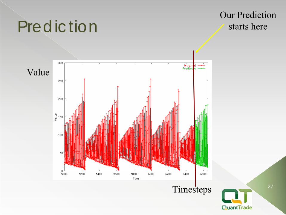
27
Prediction
Timesteps
Value
Our Prediction starts here

28
Prediction Test
Timesteps
Value
Comparison of prediction to correct values

29
Optimal Prediction
0
0.5
1
1.5
2
2.5
3
3.5
1 2 3 4 5 6 7 8 9 10 11 12 13 14 15 16 17
Frac
tal D
imen
sion
Lag
FD vs L
Our Choice
0
0.5
1
1.5
2
2.5
3
3.5
1 2 3 4 5 6 7 8 9 10 11 12 13
NM
SE
Lag
NMSE vs L
Our Choice
L(opt) = 7
Corresponding NMSE is close to optimal
Lag
NM
SE
FD

30
Speed and Scalability
Preprocessing is linear in N
Proportional to time taken to calculate FD
500
1000
1500
2000
2500
3000
3500
4000
4500
5000
2000 4000 6000 8000 100001200014000160001800020000
Pre
pro
cess
ing
Tim
e
Number of points (N)
Time vs N

31
The Fraclet Way
Our Method:
Automatically set parameters
L(opt) (answers Q1)
k(opt) (answers Q2)
In linear time on N

32
Conclusions
Black-box non-linear time series forecasting
Fractal Dimensions give a fast, automated method to set all parameters
So, given any time series, we can automatically build a prediction system
Useful in a sensor network setting

33
Pioneers in the fractal exploration of financial markets
Trading futures and options involves the risk of loss. You should consider carefully whether futures or options are appropriate to your financial situation. You must review the customer account agreement and risk disclosure prior to establishing an account. Only risk capital should be used when trading futures or options. Investors could lose more than their initial investment.
Past results are not necessarily indicative of futures results. The risk of loss in trading futures or options can be substantial, carefully consider the inherent risks of such an investment in light of your financial condition. Information contained, viewed, sent or attached is considered a solicitation for business.
Quant Trade, LLC has been a Commodity Futures Trading Commission (CFTC) registered Commodity Trading Advisor (CTA) since September 4, 2007 and a member of the National Futures Association (NFA).
Copyright @ 2012 Quant Trade, LLC. All rights reserved. No part of the materials including graphics or logos, available in this Web site may be copied, reproduced, translated or reduced to any electronic medium or machine- readable form, in whole or in part without written permission.
2 N Riverside PlazaSuite 2325Chicago, Illinois 60606Quant Trade LLC(872) 225-2110


![An Algorithm for Automated Fractal Terrain Deformation · constraining fractal terrains has been studied previously. [ST89] present a method to approximate a coarse spline mesh with](https://img.pdfslide.net/doc/110x75/5fb9c085e15ffb6a3b16e6ec/an-algorithm-for-automated-fractal-terrain-deformation-constraining-fractal-terrains.jpg)