Heterogeneous Peer Effects and Rank Concerns:Theory and Evidence

Michela M. Tincani1

June 29, 2015

1Tincani: University College London, 30 Gordon Street, London, WC1H0BE, UK,m.tincani@ucl.ac.uk. I am particularly grateful to Orazio Attanasio, Ed Hopkins, Aureo dePaula, Petra Todd and Ken Wolpin for their feedback and encouragement. I would also liketo thank Alberto Bisin, Denis Chetverikov, Martin Cripps, Mariacristina De Nardi, StevenDurlauf, Jan Eeckhout, David Figlio, Tatiana Kornienko, Dennis Kristenses, Lars Nesheim,Imran Rasul, Nikita Roketskiy, Bryony Reich, Martin Weidner, Daniel Wilhelm and par-ticipants at various seminars and conferences for insightful comments and discussions. Ithank Julia Schmieder for excellent research assistance, and Rodrigo Astroza for helpingme understand how earthquake damage propagates. Research funding from the Centre forMicrodata Methods and Practice and from the European Research Council’s grant numberIHKDC-249612 is gratefully acknowledged. I am grateful to the Chilean Ministry of Edu-cation and to the Agencia de Calidad de la Educacion for access to some of the data usedin this research. The views reported here are those of the author and are not necessarilyreflective of views at the Ministry and at the Agencia

Abstract

Much evidence exists of heterogeneous and non-linear ability peer effects in testscores. However, little is known about the mechanisms that generate them andwhether this evidence can be used to improve the organization of classrooms. Thispaper is the first to study student rank concerns as a mechanism behind ability peereffects. First, it uses a theoretical model where students care about their achievementrelative to that of their peers to derive predictions on the shape of peer effects. Sec-ond, it proposes a new method to identify heterogeneous and non-linear peer effects.Third, it tests the theoretical predictions in a novel empirical setting that uses theChilean 2010 earthquake as a natural experiment. The results indicate that rankconcerns generate peer effects among Chilean 8th graders. An important implicationis that educators can exploit the incentives generated by academic competition whenchoosing classroom assignment rules.

KEYWORDS: Peer Effects in Education, Model of Social Interactions, Rank Con-cerns, Testing Theoretical Predictions, Natural Experiment.

1 Introduction

Peers can have very important effects on the development of one’s human capital, andthe study of peer effects is a cornerstone in the Economics of Education literature.One of the most important goals of peer effect research in education, dating at leastto the Coleman report (Coleman 1966), is to design classroom allocation rules thatimprove student outcomes. As a first step towards this goal, most of the existingresearch has been concerned with identifying and quantifying peer effects.

Estimates from linear-in-means models of the impact of average peer ability onstudent outcomes vary greatly, and many studies find no effects (Angrist 2014). How-ever, several studies that relax the assumptions of the linear-in-means model, forexample, by allowing higher moments of the peer ability distribution to matter orby allowing for heterogeneous impacts, find larger and significant peer effects in theclassroom (Sacerdote 2014).1 While this suggests that policies that regroup studentsacross classrooms may generate social gains, we still lack an understanding of themechanisms behind peer effects (Sacerdote 2011, Epple and Romano 2011). As high-lighted by the work in Carrell, Sacerdote, and West (2013), this limits our ability touse peer effect estimates to improve the organization of classrooms.

This paper proposes and tests a new mechanism of social interactions in the class-room that can help us understand some of the existing evidence, as well as serveas a framework for future research on peer regrouping policies. First, it developsa theoretical model that has implications for the shape of peer effects. Second, itproposes a new method to identify heterogeneous and non-linear peer effects. Third,it tests the theoretical predictions in a new empirical setting that uses the Chilean2010 earthquake as a natural experiment. In doing so, it empirically distinguishesthe proposed mechanism from alternative ones.

In the model I propose, peer effects arise because of standard technological spill-overs operating through the mean of peer ability, and because students have rankconcerns. While students in various countries have been found to care about their rank

1For example, in a widely cited work using data from North Carolina, Hoxby and Weingarth(2005) calculate that increasing by ten percentage points the fraction of low-achievers in a classroomincreases low-achievers’ test scores by 18.5 percent of a standard deviation, while increasing bythe same amount the fraction of high-achievers increases high-achievers’ test scores by a staggering40 percent of a standard deviation. For comparison, increasing teacher quality by one standarddeviation or reducing class size by ten students increases student test scores by 10 percent of astandard deviation (Rivkin, Hanushek, and Kain 2005).

1

(Tran and Zeckhauser 2012, Azmat and Iriberri 2010), this is the first paper to studyrank concerns as a mechanism underlying peer effects. In the model, achievementis produced through costly effort. Students are heterogeneous in terms of abilityto study, which reduces the cost of exerting effort. Intuitively, how much effortstudents exert to improve their rank depends on the ability composition of theirpeers. The model is based on the theory of conspicuous consumption in Hopkinsand Kornienko (2004). The main model prediction is that making peer ability moredispersed benefits some students and harms others depending on their ability and onthe type of rank preference. The model has also the implication that achievement ismonotone decreasing in cost of effort.

To test the main model prediction, an exogenous change in peer ability varianceis needed. The key identification problem with observational data is that class-rooms with different student compositions are different also in other unobservedways that make it impossible to separate peer effects from other confounding ef-fects (Manski 1993).2 The key identification idea is that, as I document, the impactsof the Chilean 2010 earthquake were heterogeneous even across students in the sameclassroom, because the earthquake affected households differently depending on theirdistance from the rupture. To the extent that damage to a student’s home affectsa student’s ability to study, classrooms that have different distributions of damageshave also different distributions of students’ ability to study. Therefore, the effect ofthe variance of ability to study on achievement can be obtained by comparing class-rooms that are identical except for the variance in damages. Importantly, I show thatthese comparisons are free of the typical confounding factors that would arise if weused variation in any other determinant of a student’s ability to study. For exam-ple, while in classrooms with different variances in initial achievement teachers mayteach differently (Duflo, Dupas, and Kremer 2011), thus confounding the peer effectestimates, I do not find evidence that teachers adapt their teaching to the variance

2To overcome the problem of correlated effects, some studies have used data with random allo-cation of students to dorms. See, for example, Sacerdote (2001), Zimmerman (2003), Stinebricknerand Stinebrickner (2006), Kremer and Levy (2008), and Garlick (2014). In contrast, as noted in thesurvey by Epple and Romano (2011), very few experiments with random or quasi-random allocationto classrooms exist (Duflo, Dupas, and Kremer 2011, Whitmore 2005, Kang 2007). Notice that totest the model’s implications it is sufficient to identify contextual/exogenous effects in the terminol-ogy of Manski (1993), i.e. the effect on own outcomes of pre-determined classmate characteristics(ability to study). In particular, it is not necessary to identify endogenous peer effects (the effectof peer outcomes on own outcomes), which generate a simultaneity problem known as the reflectionproblem.

2

in damages. Natural disasters have been used before to identify peer effects.3 Thisstudy differs from previous work because it uses a continuous rather than a binarymeasure of exposure.

In terms of data construction, I use results from the structural engineering lit-erature to build a measure of damage to each student’s home caused by the 2010Chilean earthquake. The measure is based on seismic intensity according to theMedvedev-Sponheuer-Karnik scale. I then merge this dataset with four waves of alarge administrative dataset with information on students, teachers, classrooms andschools (Sistema de Medicion de la Calidad de la Educacion, SIMCE 2005, 2007,2009, 2011). The resulting dataset contains two cohorts, observed before and afterthe earthquake, of 110, 822 students divided into 3, 712 classrooms.

I build an econometric model that exploits the natural experiment to estimatethe heterogeneous impact on achievement of the variance in ability to study. Forthis purpose, I combine a semiparametric single-index model with a kernel-weighteddifference-in-differences estimator. This model has several desirable features. Thesemiparametric approach imposes minimal assumptions on the technology of testscore production. This allows me to test the main model’s prediction (by detectingany pattern of heterogeneity in the peer effects across students), as well as to testthe additional model prediction of monotonicity of the production technology. More-over, the difference-in-differences approach accounts for an artifact introduced by thenatural experiment; the variance in damages is determined by the geographic disper-sion of the students in the class, which could be correlated with unobserved studentand/or classroom characteristics that could confound the peer effect estimates. Forthis reason, I use the pre-earthquake cohort of students (2005-2009), who were not af-fected by the earthquake, to estimate and difference out any potentially confoundingcorrelation between geographic dispersion and outcomes.

As a preliminary data analysis, I provide the first evaluation of the impact ofthe Chilean earthquake on student test scores. Using difference-in-differences value-added test score regression models, I estimate that being exposed to the earthquakereduced test scores by 0.05 standard deviations (sd) (p-value< 0.001). Moreover,every USD 100 in earthquake damages caused a reduction of 0.016 sd in test scores(p-value< 0.001).

3In the educational peer effects literature see, for example, Cipollone and Rosolia (2007), Imber-man, Kugler, and Sacerdote (2012), and Sacerdote (2008).

3

The main empirical finding is that increasing the variance of peer ability to studybenefits low-ability students, harms middle-ability students, and it harms high-abilitystudents in Spanish classes while it benefits those in Mathematics classes. While theserich empirical patterns are hard to rationalize with standard models of peer effects, theparsimonious theoretical model can explain them in a simple and intuitive way. Low-ability students exert more effort in classrooms with larger ability variance becausethere are more students close to their ability level, therefore, surpassing the studentnext up in the ability distribution is less costly. As a consequence, middle-abilitystudents face stronger competition from below and this gives them an incentive toexert more effort. However, they also have an incentive to exert less effort, because inclassrooms with larger ability variance there are fewer students close to their abilitylevel, therefore, surpassing the student next up in the ability distribution is morecostly. The model predicts that the incentive to decrease effort prevails for middle-ability students, yielding lower test scores as observed in the data. Also high-abilitystudents face two opposing incentives, and the model predicts that test scores increasein Mathematics and decrease in Spanish, as observed in the data, whenever the rankpreference is stronger in Mathematics than in Spanish. Statistical tests do not rejectany of the theoretical model’s implications.

The implications for the estimation of peer effects are far-reaching. When thereare rank concerns, peer effects operate through the entire distribution of ability.Commonly used empirical models that focus on the mean of peer ability may failin out of sample predictions, like in Carrell, Sacerdote, and West (2013), and theymay fail to detect peer effects when these are present.4 This is especially relevantwhen peer effects are assumed to imply clustering of outcomes around the mean,an assumption often made in variance contrast methods (Glaeser, Sacerdote, andScheinkman 1996, Graham 2008). Rank concerns generate peer effects without nec-essarily implying outcome clustering.

There are also important implications for ability tracking, the most important peerregrouping policy. A common concern is that assigning students of similar ability to

4In a related paper, Tincani (2014), I show that all the (puzzling) results of the peer regroupingexperiment in Carrell, Sacerdote, and West (2013) can be rationalized by the model presented inthis paper. The model can also explain similar results from the recent peer regrouping experiment inBooij, Leuven, and Oosterbeek (2014). To the best of my knowledge, these are the only two studieswith peer regrouping experiments at the classroom/study group level, and that generate peer effectsthat are believed to be due to peer-to-peer interactions rather than peer-to-teacher interactions.

4

the same classroom harms low-ability students, who are tracked with other low-abilitystudents, unless teachers teach more productively in more homogeneous classrooms.This concern is founded when only the mean of peer ability matters for peer-to-peer interactions, which is not the case if students have rank concerns.5 In fact,under the type of rank concerns for which I find evidence in the data, students intracked classrooms have a stronger incentive to exert effort. Intuitively, competingis easier amongst equals. Therefore, this paper uncovers a new channel of operationof tracking policies. The practical implication of this result is that educators canexploit the student incentives generated by classroom assignment policies to motivatestudents. It would be helpful for future research to collect measures of student rankconcerns and use them to investigate the optimal organization of classrooms.6

The rest of the paper is organized as follows. Section 2 reviews the most relevantliterature, section 3 presents the theoretical model, and it is followed by section4 that describes the data and the context in which the theory is tested. Section5 introduces the main empirical framework, and section 6 presents the estimationresults and links them to the theoretical predictions. Robustness and alternativemechanisms are discussed in section 7, and section 8 concludes.

2 Literature Review

This is the first paper to study and find evidence of rank concerns as a mecha-nism underlying peer effects.7 Relatively few studies explore the mechanisms behindpeer effects. Lavy and Schlosser (2011) and Lavy, Paserman, and Schlosser (2012)

5Duflo, Dupas, and Kremer (2011) run an experiment where Kenyan first-graders are randomlyallocated to tracked and non-tracked classrooms and find beneficial impacts of tracking on studentsof all ability levels. They attribute those positive impacts to teachers and find supporting evidencefor this. While rank concerns are unlikely to be driving their results, the linear-in-means model ofpeer effects that they adopt rules out ex ante that peer-to-peer interactions can generate positiveeffects in the low-ability track.

6Future research could further analyze how the incentives generated by peer composition interactwith those provided through the grading system or through merit fellowships and financial awards.See Dubey and Geanakoplos (2010) for a theoretical analysis of the grading system incentives. Alarge number of studies analyze students’ response to merit and financial incentives (Angrist andLavy 2009, Kremer, Miguel, and Thornton 2009, Fryer 2010, Levitt, List, and Sadoff 2011, Cotton,Hickman, and Price 2014).

7The idea that rank concerns could generate peer effects dates back to at least Jencks and Mayer(1990) who, however, do not explore it. Related to this idea are the works of Murphy and Weinhardt(2014) and Elsner and Isphording (2015), who empirically analyze the importance of past class rankfor future performance in school.

5

use teacher and student surveys to understand how gender variation and proportionof low-ability students impact class outcomes. Using a different approach, Blume,Brock, Durlauf, and Jayaraman (2014) and Fruehwirth (2013) provide microfoun-dations to the widely used linear-in-means peer effect specification, proving that itcan be rationalized by a desire to conform. De Giorgi and Pellizzari (2013) developand test behavioral models that can rationalize observed outcome clustering withinclassrooms at Bocconi University.8 This paper uses a different and novel approach:it first presents a plausible mechanism of interactions in the classroom, and then de-rives testable implications for the shape of the peer effects. By testing the model andruling out alternative mechanisms, this is one of the first papers to investigate howclassroom composition affects student incentives.9 As emphasized in the survey inEpple and Romano (2011), modeling “the way in which students, teachers, and prin-cipals are affected by the incentives created by differing administrative assignmentsof students to peer groups” is a necessary first step to identify the optimal design ofclassrooms.

This paper focuses on the dispersion of ability in the classroom. Previous researchhas found that ability dispersion plays an important role in determining studentachievement. See, for example, Carrell, Sacerdote, and West (2013), Booij, Leuven,and Oosterbeek (2014), Lyle (2009), Duflo, Dupas, and Kremer (2011), Ding andLehrer (2007), Hoxby and Weingarth (2005), Vigdor and Nechyba (2007).10 Inter-estingly, linear-in-means models appear better suited to capture peer effects in socialbehaviors such as crime and smoking (Sacerdote 2014). Through the lens of thispaper’s finding, this can indicate that a desire to conform might be a more plausibleexplanation for this kind of social behaviors than for test scores.

By uncovering a new possible channel of operation of tracking policies, this paperis related to the literature on ability tracking. With the exception of Garlick (2014),who studies tracking in university dorms, all studies of ability tracking that use ran-

8See also Calvo-Armengol, Patacchini, and Zenou (2009), who provide microfoundations to theKatz-Bonacich centrality measure in a network.

9To the best of my knowledge, only Todd and Wolpin (2014) analyze how student incentivesare affected by the ability composition of one’s peers without requiring that the resulting reduced-form peer-effect specification be linear-in-means. Fu and Mehta (2015) analyze how parental effortdecisions are affected by tracking, and assume that peer spill-overs are of the linear-in-means type.The structural models in these papers, however, are not tested, rather, they are estimated.

10See also Benabou (1996) for a theoretical analysis of the role of the variance of the peer abilitydistribution, and Lavy, Silva, and Weinhardt (2012) for a recent analysis of nonlinear peer effects.

6

domized experiments find that they are beneficial to students. While Duflo, Dupas,and Kremer (2011) attribute this positive impact to teachers in Kenyan schools, ben-eficial impacts of tracking due to peer-to-peer interactions have been found amonglow- and middle-ability students at the University of Amsterdam (Booij, Leuven, andOosterbeek 2014), and among middle-ability students at the U.S. Air Force Academy,who were the only ones to be effectively tracked by the authors’ intervention (Carrell,Sacerdote, and West 2013).11

3 A Theoretical Model of Social Interactions

I propose a simple theory of social interactions in the classroom and derive implica-tions that can be tested empirically. The main implication is a comparative staticsresult on the effect of changing the ability variance in the classroom while keeping theability range constant, which is the type of data variation generated by the naturalexperiment. Tracking changes classroom ability variance by reducing the classroomability range instead. An advantage of my research approach is that I can investigatetracking even though I do not observe data variation akin to tracking. To do so, Ifirst identify what type of rank preferences my data are compatible with. I then usethe theoretical model under those preferences to infer how student incentives wouldbe affected by tracking.

The model is an application of the theory of conspicuous consumption in Hopkinsand Kornienko (2004), where individuals choose how much of their income to spendon a consumption good and how much on a positional good. Here, achievement is atthe same time a consumption good and a positional good, and it can be produced ata cost. Specifically, students in a classroom choose how much costly effort e to exert,and effort increases achievement/test score y. Students are heterogeneous in terms ofability, i.e., how costly it is for them to exert effort.12 The main model assumptionsare the following:A.1 Students’ utility is increasing in own achievement.

11Using non-experimental approaches, Betts and Shkolnik (2000) and Lefgren (2004) find littleevidence of benefits from tacking, while Lavy, Paserman, and Schlosser (2012) find that high-abilitystudents benefit from other high-ability students and do not help average students.

12This corresponds to income heterogeneity in Hopkins and Kornienko (2004). Alternatively,students can be assumed to be heterogeneous in terms of how productive their effort is, and, underminor modifications to the assumptions on the utility function, the model would have the sameimplications.

7

A.2 There are technological spill-overs in the production of achievement, i.e., meanpeer ability directly affects own achievement.A.3 Students’ utility is increasing in rank in terms of achievement.

Assumptions A.1 and A.2 are standard.13 Assumption A.2 gives rise to exogenouspeer effects (Manski 1993). Assumption A.3 is novel in the theoretical literatureon educational peer effects. It introduces a competitive motive and it gives rise toendogenous peer effects (Manski 1993), because how much effort each student exertsis determined endogenously by the equilibrium of a game of status between students.

Students differ in terms of a type c: those with a higher c incur a larger cost ofeffort. Type c captures any student characteristics, physical or psychological, thataffect her ability to study, such as cognitive skills, access to a computer or books,availability of an appropriate space for studying, parental help, etc. Notice thatability reduces c. Type c is distributed in the classroom according to c.d.f. G(·) on[c, c]. Each student’s type c is private information, but the distribution of c in theclassroom is common knowledge.

An appeal of the model is that it does not make distributional assumptions and,whenever feasible, functional form assumptions. However, some plausible shape re-strictions are imposed to prove the results. The cost of effort is determined by anincreasing and strictly quasi-convex function in effort q(e; c). Higher types c incurhigher costs for every level of effort e, i.e. ∂q(e;c)

∂c> 0 for all e. Moreover, at higher

types the marginal cost of effort is (weakly) higher: ∂2q(e;c)∂c∂e

≥ 0.Effort determines achievement according to the production function y(e) = a(µ)e+

u(µ), where µ is the classroom mean of c. Parameters a(µ) and u(µ) capture techno-logical spill-overs working through the mean of peer ability (assumption A.2). Thesecan be indirect, i.e., working through the productivity of classroom specific factors,or direct, i.e. due to peer-to-peer contacts. An example of an indirect spill-over isteacher productivity depending on students’ average abilities. An example of a directspill-over is more able peers (lower µ) asking relevant questions in class and, in sodoing, facilitating their classmates’ learning. Notice that the model is flexible in thatit allows these technological spill-overs to affect both the level of achievement (u) andthe productivity of effort (a).

13For example, Blume, Brock, Durlauf, and Jayaraman (2014), Fruehwirth (2012), and De Giorgiand Pellizzari (2013) assume that student’s utility is increasing in own achievement. Several papersmodel technological spill-overs as operating through mean peer characteristics, e.g. Arnott andRowse (1987), Epple and Romano (1998), Epple and Romano (2008).

8

The utility function can be decomposed into two elements: a utility that dependsonly on own test score y and effort cost q, V (y, q), embedding assumption A.1; anda utility that depends on rank in terms of achievement, embedding assumption A.3.The utility from achievement is non-negative, increasing and linear in achievement,decreasing and linear in q, and it admits an interaction between utility from achieve-ment and cost of effort such that at higher costs, the marginal utility from achievementis (weakly) lower (V12 ≤ 0).14 No specific functional form assumptions are made onq(·) and on the interaction between y and q, therefore, results from the model arevalid under a broad class of preferences. For example, more able peers (lower c) may(or may not) have higher marginal utilities from achievement.

The student’s classroom rank in terms of achievement is given by the c.d.f. ofachievement computed at a student’s own achievement level, FY (y). This is thefraction of students with achievement lower than one’s own, and it is a standardway to model rank in theoretical models of status seeking (Frank 1985). Becauseachievement is an increasing and deterministic function of effort, rank in achievementis equal to rank in effort: FY (y) = FE(e). The utility from rank, S(FY (y)), is equalto FE(e) + φ, where φ is a non-negative constant.

Overall utility U(y, q; c) is the product of utility from own achievement V (y, q; c)and utility from rank S(FY (y)): V (y, q; c) (FE(e) + φ). The parameter φ determinesthe type of rank concerns that students have. When φ > 0, students have a minimumguaranteed level of utility even if they rank last (FE(e) = 0). On the other hand,when φ = 0 ranking low has dire consequences, and this will generate that studentsclose to the bottom of the ability distribution will be desperate to avoid a low-rank.Because the two cases (φ = 0 and φ > 0) yield different testable implications, to theextent that I do not reject the model, I can identify which type of rank concerns iscompatible with the data.Each student chooses effort to maximize overall utility. Focusing on symmetric Nashequilibria in pure strategies, and assuming that the equilibrium strategy e(c) is strictlydecreasing and differentiable with inverse function c(e), rank in equilibrium can berewritten as 1 − G(c(ei)), and i’s utility as V (y(ei), q(ei, ci))(1 − G(c(ei))).15 The

14All results are valid under an alternative set of assumptions for the utility from achievement.These are: strictly quasi-concave utility of achievement, decreasing and linear utility from cost ofeffort (V2 < 0, V22 = 0) with a linear cost function (d

2qd2e = 0) and additive separability between

utility from achievement and cost of effort (V12 = 0).15The probability that a student i of type ci with effort choice ei = e(ci) chooses a higher effort

9

first-order condition then is:

V1

Mg. increase in achiev.︷︸︸︷a(µ)︸ ︷︷ ︸

mg. ut. from increased achiev.

+ V (y, q)1−G(c(ei)) + φ

Mg. increase in rank︷ ︸︸ ︷g(c(ei))(−c

′(ei))︸ ︷︷ ︸

mg. ut. from increased rank

= −V2∂q

∂e︸ ︷︷ ︸mg. cost

(1)

and it implies the first-order differential equation reported in equation 7 in OnlineAppendix A.1. The solution to this differential equation is a function e(c) that isa symmetric equilibrium of the game. The assumptions on the utility function, onthe cost of effort function and on the achievement production function guaranteethat the results in Hopkins and Kornienko (2004) apply under appropriate proofadaptations.16 In particular, while the differential equation does not have an explicitsolution, existence and uniqueness of its solution and comparative statics resultsconcerning the equilibrium strategies can be proved for any distribution functionG(c) twice continuously differentiable and with a strictly positive density on someinterval [c, c], with c ≥ 0. The first theoretical result is summarized in the followingProposition:

Proposition 3.1 (Adapted from Proposition 1 in Hopkins and Kornienko (2004)).The unique solution to the differential equation (7) with the boundary conditionse(c) = 1

cfor φ = 0 and e(c) = enr(c) for φ > 0, where enr solves the first order condi-

tion in the absence of rank concerns (V1a(µ)|e=enr = −V2∂q∂e|e=enr), is an (essentially)

unique symmetric Nash equilibrium of the game of status. Equilibrium effort e(c) iscontinuous and strictly decreasing in type c.17

than another arbitrarily chosen individual j is F (ei) = Pr(ei > e(cj)) = Pr(e−1(ei) < cj) =Pr(c(ei) < cj) = 1 − G(c(ei)), where c(·) = e−1(·). The function c maps ei into the type cithat chooses effort ei under the equilibrium strategy. Strict monotonicity and differentiability ofequilibrium e(c) are initially assumed, and subsequently it is shown that equilibrium strategies musthave these characteristics.

16To guarantee existence of an equilibrium when φ = 0, one additional assumption must be made:each student has an upper bound on achievable test score, and students with higher ability (lowerc) have a higher upper bound. For example, a student of type c can never achieve more thany = a(µ) 1

c + u(µ). Under this technological constraint, no student of type c will exert more effortthan 1

c , because any unit of effort above this level does not increase achievement, but it is costly.Footnote 17 explains how this guarantees existence. One of the main differences with the model inHopkins and Kornienko (2004) is that here equilibrium strategies e(c) are decreasing in c, whereasthere they are increasing. See the procurement auctions model in Hopkins and Kornienko (2007) foranother example of decreasing strategies.

17The equilibrium is essentially unique, in the sense that the only source of multiplicity is at thepoint c when φ = 0. In a symmetric equilibrium, the student with the highest cost, c, has rank 0when φ = 0. Her equilibrium utility is 0, and the only way she can increase it is by increasing her

10

Proof: see Online Appendix A.1.Notice that Proposition (3.1) rules out the case in which for large enough valuesof c students exert more effort. This would be akin to a backward-bending laborsupply curve.18 Because this result may appear restrictive, I empirically test it. Theimplication can be rephrased in terms of achievement, given that achievement is anincreasing function of effort, to obtain the first testable implication:Testable Implication 1: Achievement is decreasing in type c.

Now consider two distributions, GA(c) and GB(c), that are such that they havethe same mean, and GB has larger dispersion than GA in the Unimodal LikelihoodRatio sense (GA �ULR GB), defined in Online Appendix A.1. This happens when,for example, GB is a mean-preserving spread of GA. In informal terms, one canshow that the effect of moving from GA to GB is heterogenous across individuals,depending on a student’s rank in terms of c, and it depends on φ, i.e., on the type ofrank concerns.19 This result provides the second testable implication of the model:Testable Implication 2: If students are averse to a low rank (φ = 0), then whenthe dispersion of c increases, either all students perform more poorly, or all studentsexcept low-c (high-ability) students do more poorly. If students are not averse to a lowrank (φ > 0), then when the variance of c increases, middle-c students perform morepoorly and high-c (low-ability) students perform better, while low-c (high-ability)students may perform better or worse. These patterns are represented graphically inFigure 1.

rank above 0. Therefore, for a strategy profile to be an equilibrium, it must be that the studentwith a slightly lower cost c exerts an amount of effort that is such that the least able student, c,is unable to increase her rank by exerting more effort. Therefore, in equilibrium limc→c− e(c) = 1

c ,where 1

c is the maximum effort that student c can exert (see footnote 16), and the least able studenthas rank 0 and is indifferent between any level of effort between 0 and 1

c .18For example, if the marginal utility from achievement tends to infinity as achievement approaches

its lower bound, then it is not necessarily the case that students with a larger cost of effort exert lesseffort than those with a lower cost of effort. This is because for students with achievement close tothe lower bound, decreasing effort would have a large cost in terms of utility. This is akin to incomeand substitution effects in labor supply: as the cost of effort increases, the substitution effect wouldinduce individuals to exert less effort, but the income (in this case, achievement) effect would inducethem to exert more effort to distance themselves from the achievement lower bound.

19The formal statement of the comparative statics result can be found in Proposition (A.1) inOnline Appendix A.1.

11

Dy(c)

c0

Dy

Dy(c)

c0

Dy

(a) φ > 0, no aversion to alow rank

Dy(c)

c0

Dy

Dy(c)

c0

Dy

(b) φ = 0, aversion to alow rank

Figure 1: The function Dy(c) traces the effect on achievement of increasing thevariance of c, as a function of student type c. In the φ > 0 case, it can cross thex-axis once or twice. If it crosses it once (upper panel a), the sequence of its signs,from low c to large c, is −, +. If it crosses it twice (lower panel a), the sequence ofits signs, from low c to large c, is +, −, +. In the φ = 0 case, it can cross the x-axisat most once. If it does not cross it (upper panel b), it must lie below it. If it crossesit (lower panel b), the sequence of its signs, from low c to large c, is +, −.

12

3.1 Model Intuition and Discussion of Assumptions

Intuition. Rank preferences imply that each student’s incentives are affected by thefraction of peers below her ability, at her ability, and above her ability. First, as canbe seen from the first order condition in 1, the marginal utility from increasing one’sown rank depends positively on the density at one’s own type c, g(c). Intuitively, themore students there are of a similar type c to one’s own (i.e., the larger this density),the more students can be surpassed in rank by exerting effort. Conversely, when fewerstudents can be surpassed for the same amount of effort, students have an incentiveto “give up.”

Second, the first order condition in 1 shows also that the marginal utility fromincreasing one’s own rank increases when the fraction of less able students (i.e., 1 −G(c)) decreases, and the extent of this increase depends on φ. This derives from themultiplicative specification of preferences, which implies that not only the utility fromrank, but also the enjoyment of one’s own absolute level of achievement is lower atlower ranks. The closer the students are to the bottom of the ability distribution (i.e.,to c), the fewer classmates there are with whom they can make favorable comparisons,and the stronger their incentive to exert effort to avoid a low achievement rank is.The comparative statics result indicates that this incentive is strongest when φ = 0.For this reason, I call φ = 0 the case of aversion to a low rank.

The comparative statics result is the net effect of these two incentives, which varieswith a student’s ability c and with the type of rank concerns (φ = 0 or φ > 0). Fig-ure 2 shows two ability distributions G(c) with different variances. As the varianceincreases, the density increases at the tails and decreases in the middle, therefore,irrespective of the value of φ, low- and high-c students have an increased incentiveto exert effort and middle-c students have a lower incentive to exert effort. However,high-c students now face a larger fraction of less able students (1−G(c)), which de-creases their incentive to exert effort to avoid a low rank. Hence, high-c students facetwo opposite incentives. The model predicts that they reduce their effort when φ = 0and increase it when φ > 0. Middle-c students have an incentive to lower their effortunder both φ = 0 and φ > 0. This is because when φ = 0 they face less competitionfrom the less able students, while when φ > 0 they face more competition from theless able students, but the model predicts that the incentive to reduce effort due tothe lower density at their c level prevails. Under both φ = 0 and φ > 0, low-c stu-dents face two opposite incentives: the incentive to increase their effort due to the

13

fatter tail at their end of the distribution, and the incentive to decrease their effort,because they face less competition from middle-c students and, therefore, they canreduce their effort cost without reducing their rank. Which effect prevails dependson how strong the preference for status is relative to the utility from achievementnet of the effort cost. This is determined by V (·) and q(·), on which the model doesnot make specific functional form assumptions. Intuitively, a stronger preference forstatus leads to an increase in outcomes for low-c students, because the incentive toimprove their rank prevails over the incentive to pay a lower effort cost.20

Discussion of assumptions. The assumption that overall utility is multiplicative inprivate utility V and social utility S may appear counterintuitive. However, thisassumption makes the problem’s structure similar to that of a first-price sealed-bidauction, where expected payoff is the product of the value of winning (V ) and theprobability of winning (F ). As noted in Hopkins and Kornienko (2004), “it is this for-mal resemblance to an auction that permits clear comparative statics results.” Whileit would be desirable to relax this assumption in favor of more general preferencespecifications, such a purely theoretical contribution would go beyond the scope ofthis paper. This paper is the first to apply existing theoretical tools in the rank con-cerns theoretical literature to the field of peer effects in education, and to test themin this context. Future extensions could specify less restrictive preferences and resortto numerical rather than analytical model solution tools.

Rank concerns can be modeled in many ways. As in Hopkins and Kornienko(2004), I consider only two (φ > 0 and φ = 0). While this is restrictive, these two casesalone can explain important and diverse evidence. Recent laboratory experimentsshow that individuals are averse to a low-rank, as predicted by the model whenφ = 0 (Kuziemko, Buell, Reich, and Norton 2014). Moreover, Tincani (2014) showsthat the model with φ = 0 can explain all of the (unexpected) results of the peerregrouping experiment in Carrell, Sacerdote, and West (2013), as well as more recentexperimental evidence (Booij, Leuven, and Oosterbeek 2014). The case of φ > 0, onthe other hand, can explain this paper’s empirical evidence.

20For example, it can be shown that if overall utility was (y(e)−e)α (F (e) + φ), then low-c studentswould increase their effort when status has a larger weight than achievement net of effort cost (α < 1)and decrease it otherwise (α ≥ 1).

14

Figure 2: Type distributions in two classrooms, and cutoffs separating low-, middle-and high-c students.

15

t

2005 2007 2009 2010 2011Earthquake

Cohort PRE

Cohort POST

Figure 3: Data time-line.

4 Data and Earthquake

Data. I use two cohorts of students from the SIMCE dataset (Sistema de Medicionde la Calidad de la Educacion). For both cohorts I observe the universe of 8th gradestudents, for whom I have information on current and 4th grade Math and Spanishstandardized test scores, father’s and mother’s education, household income, gender,and town of residence. Classroom level information includes class size, and the expe-rience, education, tenure at the school, gender, and type of contract of both Spanishand Math teachers.

One cohort is observed in the 8th grade in 2009, before the 2010 earthquake, whilethe other cohort is observed in the 8th grade in 2011, after the earthquake, as shown inFigure 3. For both cohorts, identifiers are available at the student, teacher, classroomand school level. This makes this dataset ideal for the study of social interactions,because each student’s classmates, as well as their school and Math and Spanishteachers, can be identified.

Finally, I obtained from the Chilean Ministry of Education a list of schools thatclosed as a consequence of the earthquake.21 I use this list to identify evacuees (i.e.,the students who attended the schools that closed), as well as the schools that theymoved to. I drop from the sample the 5, 988 evacuees thus identified, and the 803schools receiving at least one of them, to rid my estimates of any peer effect arisingfrom changes to classroom composition induced by the arrival of evacuees.22

Earthquake. Just a few days before the start of the new school year, on February 27th

21They closed either because their buildings became unsafe, or because most of the students’ homeswere so badly damaged, that students had to relocate and the schools had too low attendance.

22This distinguishes the identification strategy in this paper from that in Imberman, Kugler, andSacerdote (2012), where the influx of Katrina evacuees is used as an exogenous source of changeto classroom composition. Unlike the case of Katrina, evacuees in Chile were spread across a largenumber of schools. Therefore, each receiving school received only a small influx of evacuees, toosmall to detect any statistically significant impact.

16

Figure 4: Source: Comerio (2013). Handmade sign found in Cauquenes, Chile, onFebruary 2, 2012. Translation: “Reconstruction is like God. Everyone knows it exists,but nobody has seen it.”

2010, at 3.34 am local time, Chile was struck by a magnitude 8.8 earthquake, the fifth-largest ever instrumentally recorded (Astroza, Ruiz, and Astroza 2012). Shaking wasfelt strongly throughout 500 km along the country, covering six regions that togethermake up about 80 percent of the country’s population. The damage was widespread;370, 000 housing units were damaged or destroyed. The government implemented anational reconstruction plan to rebuild or repair 220, 000 units of low- and middle-income housing. Estimated total costs are around $2.5 billion. By the time theSIMCE 2011 sample was collected, i.e., 20-22 months after the earthquake struck,despite impressive efforts by the Government, only 24 percent of home reconstructionhad been completed (Comerio 2013). This led to frustration in the population, asshown in Figure 4.

To explore how damages are distributed in my sample, I use the geographicalcoordinates of the town of the school and of the town of the home of each student tobuild a measure of local earthquake intensity at each school and student’s home. Todo so, I apply the intensity propagation formula (Astroza, Ruiz, and Astroza 2012),which yields seismic intensity on the Medvedev-Sponheuer-Karnik (MSK) scale as afunction of a town’s distance from the earthquake’s main asperity, i.e., the point onthe fault where the rupture starts.23 MSK intensity indicates the extent of damage

23How earthquake damage propagates depends on the geological features of the affected area,therefore, structural engineers estimate this formula for each earthquake separately. First, theyobserve damages in a sample of towns, then, they estimate the parameters of a non-linear regression

17

observed in the buildings of a given town. The same MSK intensity corresponds todifferent levels of damage depending on the type of construction. However, conditionalon a construction type, intensity can be mapped back into a specific level of damage.For example, in towns with low MSK intensity, 5, adobe constructions suffered onaverage damages for $20, while at the strongest intensity, 9, damages per adobeconstruction were on average $13, 800.24 House type is not observed in my dataset.However, Astroza, Ruiz, and Astroza (2012) report that the ∼ 60% poorest Chileanslive in one of two house types with very similar earthquake resistance: old traditionaladobe constructions (6.1%) and unreinforced masonry houses (51.9%). Given thestriking school stratification in Chile, with public school students belonging to thepoorest ∼ 50% of Chilean households, it is reasonable to expect that all public schoolstudents live in one of these two building types. To avoid measurement error due tohouse type unobservability, I restrict my sample to public school students. Finally,the main empirical analysis includes only students in the regions affected by theearthquake. The resulting sample contains observations on 110, 822 students, 2, 579schools and 3, 712 classrooms.

Astroza, Ruiz, and Astroza (2012) report that even towns that are close to eachother were subject to very different levels of seismic intensity. For example, LasCabras and Pichidegua are only 4.87 miles apart. In Las Cabras, the worst damagesuffered by adobe houses has been moderate, ranging from fine cracks in the wallsto the sliding of roof tiles, whereas in Pichidegua some adobe houses were destroyed.This suggests that in classrooms with students from different towns, we may observethat students’ homes suffered different levels of damages, even though students in thesame school tend to live in towns that are close to each other. In fact, in classroomswhere not all student reside in the same town, the average standard deviation in dam-ages is approximately USD 350, corresponding to 92 percent of the average monthlyincome. Of all classrooms in the regions affected by the earthquake, 48 percent arenot composed of students who all reside in the same town. The map in Figure 4

of damage on distance from the asperity. For the 2010 Chilean earthquake, the estimated formulais I(∆A) = 19.781− 5.927 log10(∆A) + 0.00087∆A, where I is MSK intensity and ∆A is distance inkilometers from the main asperity. The R2 is 0.9894. Refer to the Online Supplementary Materialfor an explanation of how each sampled town is assigned an MSK intensity.

24See the Online Supplementary material on the author’s website for details on how the recon-struction costs are calculated. Table 4 in Online Appendix A.2 shows reconstruction costs foradobe structures by MSK intensity, and Figure A.2 reports pictures of adobe houses that suffereddifferent grades of damage.

18

Figure 5: Schools that attract students from different towns, and within school stan-dard deviation in damages.

plots these schools, and it indicates the standard deviation of damages within eachschool. As can be seen, there is considerable variation within and across schools. Thisvaluable variation provides the basis for testing the model.

4.1 Descriptive Statistics and Preliminary Data Analysis

The modal damage in the sample is USD 365, with a mean of USD 950 and a standarddeviation of USD 1, 480. Table 1 presents other sample descriptive statistics. Theregions affected by the earthquake are poorer than those not affected. The mainempirical analysis uses only earthquake regions. While one may worry that seismicintensity is correlated with student unobservable characteristics affecting outcomes,I show below that conditional on student observable characteristics, seismic intensityis uncorrelated with student outcomes.

I present the first evaluation of the effect of the 2010 Chilean earthquake on

19

Table 1: Sample descriptive statistics

Earthquake Regions Non-Earthquake RegionsMean St Dev Mean St Dev

Baseline Math Score -0.095 0.949 -0.114 0.910Baseline Spanish Score -0.092 0.943 -0.087 0.810Father’s Education (years) 9.646 3.338 9.892 3.289Mother’s Education (years) 9.651 3.183 9.741 3.205Monthly Household Income (USD) 363 341 430 408Class size 26.7 10.8 25.7 12.2% Classmates from same town 0.92 0.16 0.96 0.10% Classmates from same town | < 1 0.83 0.20 0.88 0.13% Classrooms with not allstudents residing in same town 0.48 0.38Math Teachers

% Female 0.55 0.52% Postgraduate Degree 0.56 0.53Teaching Experience (years) 22.0 13.5 22.8 13.2Tenure at school (years) 12.3 11.5 11.9 11.0

Spanish Teachers% Female 0.81 0.78% Postgraduate Degree 0.56 0.49Teaching Experience (years) 21.2 13.5 21.5 13.5Tenure at school (years) 12.0 11.4 11.3 10.8

20

student test scores. I exploit the fact that the pre- and post-earthquake cohortsare observed both in regions affected and not affected by the earthquake, and thatstudents are observed at two points in time, to estimate a difference-in-differences testscore value-added regression. Table 5 in Online Appendix A.3 presents estimates forall schools and by school type (municipal, private subsidized, private unsubsidized).Being exposed to the earthquake reduced test score growth, on average, by 0.05standard deviations (columns 4 and 8). This estimate is net of any individual, regionaland/or cohort effects.

To estimate the impact of the continuous measure of seismic intensity at a stu-dent’s home, Ii, I calculate MSK intensity for all students (in earthquake regions) inboth cohorts. I then estimate the following regression of test scores y of student i inclassroom l in school s and in grade g = 8 on past test score, individual characteristicsxi, and dummies for belonging to the post-earthquake cohort, Pi = 1, and living inan earthquake region, Ei = 1 (estimation results can be found in Tables 6 and 7 inthe Online Supplementary Material):

yilsg = α+ λs + yils(g−4)δ + x′iγ + PiθP +EiθE + (1− Pi)Iiθpre + PiIiθpost + εilsg. (2)

The effect of earthquake intensity on test score growth is θpost − θpre.25 I find thatincreasing earthquake intensity by one category in the MSK-scale reduces test scoregrowth by 0.008∗∗∗ standard deviations (sd) in all schools, and by 0.005∗∗∗ and 0.006∗∗∗

sd in municipal schools for Math and Spanish, respectively. This corresponds approx-imately to a reduction of 0.016 sd in test scores for every USD 100 in damages.

Finally, I find that seismic intensity at the individual student level is uncorrelatedwith unobservable student characteristics affecting outcomes. Using the unaffectedpre-earthquake cohort, I estimate a value-added regression of test scores on studentcharacteristics, classroom characteristics and on own seismic intensity, and I findthat the coefficient on the latter is not statistically different from zero (see Table 6in Online Appendix A.3).26 This indicates that, conditional on student observables,

25This technique is similar in spirit to Card (1992), with the difference that, in this context, I amable to construct treatment intensity also for the untreated pre-earthquake cohort. This allows me tomake a weaker identifying assumption than in Card (1992). In fact, the estimated treatment effecthere is consistent even if treatment intensity is correlated with unobserved student characteristicsaffecting outcomes, as long as this correlation is the same in the pre- and post-earthquake cohorts.The sample in this paper satisfies also the stronger assumption made in Card (1992), i.e. thattreatment intensity is uncorrelated with student unobservables, as explained below.

26Not surprisingly, θpre in equation 2 is also not significantly different from zero. Moreover, I

21

seismic intensity is uncorrelated with student unobservables.

5 An Empirical Model of Social Interactions

Achievement Production Function with Peer Spill-overs. I assume that a student’sachievement depends on her own characteristics and on classroom characteristics.There are peer effects because two students with identical characteristics may ob-tain different test scores in two classrooms that are identical except for the abilitycomposition of peers.

I broadly define a student’s ability to study as being determined by all individuallevel inputs into the production of achievement. I assume that it is a scalar obtainedas a single index of a vector of student characteristics. I refer to this scalar asthe student’s type, and denote it by ci. Type ci, therefore, is the linear functionci = α1xi, where xi contains student initial ability (as measured by lagged test scores),father’s and mother’s education, household income, and gender. Changes in classroomcomposition can be represented as changes in the classroom distribution of type c,Gl(c). The achievement production function of student i in classroom l is:

yil = ml(ci) + εil = e(ci;Gl(c)) + ul(ci) + νil = el(ci) + ul(ci) + νil (3)

where yil is test score of student i in classroom l. The function el(·) maps individualtype ci into achievement, and it is indexed by l because of peer effects: it dependson the distribution of c in classroom l, Gl(c). The function ul(ci) captures the (het-erogeneous) impact on test scores of all observable classroom characteristics. Theseare characteristics that are shared by all students in the classroom, and their effectmay vary by student’s type ci. Specifically, ul(ci) = u(ci, zl, Fl(xi)) where zl containsteacher experience, teacher gender, whether the school is urban or rural, and classsize; and Fl(xi) is the classroom distribution of student characteristics. The depen-dence on Fl(xi) captures the fact that teachers may teach differently depending onthe characteristics of the students in the classroom, an indirect peer effect. Finally,there may be correlated effects (Manski 1993), as E[νil|l, ci] 6= 0. In particular, thisconditional expectation is described by a function of type that depends on classroom

estimate a value-added regression similar to 2, without the regressor (1 − Pi)Ii, and I obtain acoefficient on PiIi that is very close to θpost − θpre in equation 2. See the Online SupplementaryMaterial, where the results from these regressions are presented.

22

characteristics, ψl(ci) = ψ(ci, zl, Fl(xi)), so that νil = ψl(ci) + εil with E(εil|l, ci) = 0.The shock εil is a measurement error. Correlated effects may arise because, for exam-ple, more motivated students are found in classrooms with better characteristics zl,or because certain types of teachers are assigned to classrooms with certain studentcompositions Fl(xi). In a similar spirit to ul(ci), the function ψl(ci) captures theheterogeneous impact on students of unobserved classroom characteristics. I do notmake any functional form assumptions on the functions el(·), ul(·) and ψl(·), and anydistributional assumptions on εil.

Equation 3 is a semiparametric single-index model (Hall 1989, Ichimura 1993,Horowitz 2010). I jointly estimate the ml(ci) function in each classroom l, usingkernel methods, and the α parameters.27 The estimation algorithm is presented inOnline Appendix A.4, where the details for the calculation of the standard errorsare also presented. Notice that el(ci) is not separately identified from ul(ci) + ψl(ci).Therefore, at this stage peer effects cannot be separately identified from the effect ofobserved and unobserved classroom characteristics, or, in other words, from indirectpeer effects (ul) and correlated effects (ψl).

Seismic Intensity as a Source of Identifying Variation. The ideal setting to evaluatethe direct effect of peers on test scores is one where student allocation to classrooms israndom or experimentally controlled, so that el(ci) can be independently varied fromul(ci) + ψl(ci). While college administrators sometimes adopt random assignment ofpeers to dorms, random assignment of peers to classrooms is rarely adopted in schoolsor colleges.28 Moreover, as noted in the survey by Epple and Romano (2011), exper-iments with random assignment to classrooms are rare, especially beyond primaryschool.29

Given the limited availability of this kind of data, I adopt a different approach.The goal is to vary moments of the distribution of student types in the classroom,

27I impose the restriction that ci does not depend on unobservable student characteristics, becauseallowing for an unobserved shock to affect ci would require to assume that the m(ci) function ismonotonic. I do not impose shape restrictions on m(·) because I want to test for its monotonicity,to test the first theoretical model’s implication.

28Random assignment to dorms has been used by, for example, Sacerdote (2001), Zimmerman(2003), Stinebrickner and Stinebrickner (2006), Kremer and Levy (2008), and Garlick (2014).

29One such experiment was conducted among Kenyan first graders and studied by Duflo, Dupas,and Kremer (2011). Whitmore (2005) studies peer effects among kindergartners using data fromthe project STAR experiment in Tennessee. See also Kang (2007), who studies peer effects among7th and 8th graders in Korea using a quasi-randomization.

23

Gl(c), and quantify how el(ci) is affected, net of any change in ul(ci)+ψl(ci). Varyingthe distribution of student types could be achieved by comparing classrooms withdifferent distributions of student characteristics xi. However, as ul(·) and ψl(·) dependon Fl(xi), the effect on el(ci), i.e., the peer effect of interest, would not be separatelyidentified from correlated effects and from indirect peer effects. To overcome thisobstacle, I consider a shock to each student’s type ci that is such that its distributionin the classroom, or at least a moment of this distribution, is not systematicallyrelated to unobserved classroom characteristics or to the productivity of teachers.

The shock is seismic intensity at a student’s home for students who were affectedby the 2010 Chilean earthquake, Ii. To the extent that Ii affects a student’s abilityto learn, ci, classrooms with different distributions of seismic intensity have differentdistributions of student types, even if the distributions of all other student charac-teristics, Fl(xi), are identical. This holds true independently of the channel throughwhich seismic intensity affects a student’s ability to study. One possible channel is thedisruption to the home environment. It may increase the opportunity cost of time,because students may be required to spend time helping their parents with home re-pairs.30 Additionally, students may not have access anymore to the areas of the homethat they used for doing their homework. Another possible channel involves psycho-logical well-being. The medical literature finds that earthquake exposure affects brainfunction and that it can cause Post Traumatic Stress Disorder (PTSD).31 Moreover,the severity of PTSD increases with seismic intensity (Groome and Soureti 2004).

Survey evidence suggests that seismic intensity at a student’s home did in factaffect a student’s ability to study. First, conditional on student initial ability and onparental education and income, students more affected by the earthquake report thatit is more costly for them to study, as shown in Table A.3 in Online Appendix A.3.32

30This is particularly likely to have occurred among the low-income Chilean families that mysample focuses on, because most of the government subsidies were in the form of vouchers forpurchasing the materials needed for the repairs, and families were expected to perform the repairsthemselves (Comerio 2013).

31This may last for several months after the earthquake. See, for example, Altindag, Ozen, et al.(2005), Lui, Huang, Chen, Tang, Zhang, Li, Li, Kuang, Chan, Mechelli, et al. (2009), Giannopoulou,Strouthos, Smith, Dikaiakou, Galanopoulou, and Yule (2006).

32As shown earlier, conditional on these student observables, seismic intensity is not correlatedwith unobservables affecting test scores. Therefore, I am confident that this effect can be interpretedas causal. Students were asked to rate how much they agree with sentences such as “It costs meto concentrate and pay attention in class” and “Studying Mathematics costs me more than it costsmy classmates”. I combine the answers to these questions into a single factor using factor modeling,and I estimate the impact of seismic intensity at a student’s home on this elicited measure of cost.

24

Second, I find that the negative impact of seismic intensity on test scores (see section4.1) is larger in classrooms in which the teacher assigns homework more frequently.This suggests that home damage affected the productivity of study time at home.33

Third, using a dataset collected only a few months after the earthquake, I find thatstudents affected more badly by the earthquake report reading less books.34

In the empirical model, I assume that the ability to study for the 2011 cohort ofstudents affected by the earthquake is: ci = α1xi +α2Ii+α3Iixi. The interaction termIixi captures individual heterogeneity in how seismic intensity affects a student’s typeci. For example, wealthier parents may try to attenuate the impact of the earthquakeby providing a new study environment for their child.35 As I show in detail below,I find that the variance of seismic intensity in the classroom satisfies an exclusionrestriction that allows me to use it in a similar fashion to an Instrumental Variable(IV) for variance of student types. However, unlike in the case of IV, the observ-ability of ci (and of its variance) is not required in this framework; the single-indexmodel estimates ci. Given that a student’s ability to study is not directly observed, astandard IV approach would not be feasible here because the instrumented variablewould not be observed.

Differencing out the confounding effect of geographic dispersion. Seismic intensity isbased on a student’s home location. Therefore, seismic intensity variance is posi-tively related to the geographic dispersion of the students in a classroom. Using thecohort of students that was not affected by the earthquake, I construct future seismicintensity for each student in the sample, and I find that the coefficient on seismic in-tensity variance in a test score value-added regression is large and positive, as shownin Table 6 in Online Appendix A.3. This indicates that geographic dispersion ofthe students in the classroom is (positively) correlated with student outcomes. Thiscould be because classrooms that attract students from further away have some desir-

33The additional effect is −.0173614, p-value 0.049, see Table 9 in the Online SupplementaryMaterial. The amount of homework assigned is observed only for Math classrooms in the cohort ofstudents affected by the earthquake, therefore, a difference-in-differences strategy that accounts forcohort effects cannot be adopted here.

34See Figure 4 in the Online Supplementary Material. This is compatible with an increase in costof effort/decrease in the ability to study, that was followed by a reduction in effort. This evidenceis only suggestive as it comes from a cross-section.

35The medical literature reports that the psychological impact of earthquake exposure is strongeron girls, and my parameter estimates find support for this.

25

able characteristics unobserved to the econometrician, and/or because the studentsin those classrooms are different in unobserved ways such as their motivation. Re-gardless of the nature of this correlation, if not accounted for it could confound theestimate of the peer effect of interest, i.e., of the effect of the variance of peer ability(“instrumented” by variance of seismic intensity) on own test scores.

To account for this correlation, I let the functions ul(·) and ψl(·) depend on thevariance of seismic intensity in the classroom, σ2

Il. As a result, when we compare class-rooms in the post-earthquake cohort that, ceteris paribus, suffered different levels ofvariance of seismic intensity, student outcomes are different for two reasons: directpeer effects, i.e., the variance of ci is different in these classrooms and, as a result, el(ci)is different; and geographic dispersion effects due to the fact that those classrooms aredifferent in unobserved ways (different ψl(·)) and/or their observed classroom char-acteristics have different productivities (different ul(·)). However, when we compareclassrooms in the pre-earthquake cohort that, ceteris paribus, have different levelsof variance of seismic intensity, student outcomes are different only for one reason:geographic dispersion. This is because in the pre-earthquake cohort, student abilityto study, ci, has not been affected by seismic intensity yet, therefore, variance of seis-mic intensity in the classroom is not related to variance of student ability, but onlyto geographic dispersion. This suggests an identification strategy: the geographicdispersion effects can be computed in both cohorts of students, and differenced outfrom the post-earthquake cohort.

Specifically, I model classroom effects in both cohorts as u(ci, zl, Fl(xi), Il, Il, σ2Il)

and ψ(ci, zl, Fl(xi), Il, Il, σ2Il), where Il is seismic intensity in the school’s town, Il is

the average and σ2Il is the variance of seismic intensity suffered by the students in

classroom l. I let ul(·) and ψl(·) depend on Il and Il, and not just on σ2Il, for two

reasons: first, to allow for the fact that actual seismic intensity at the school andaverage intensity of the students in the classroom can directly impact the outcomesof the student in the post-earthquake cohort (e.g. through the damage to schoolfacilities); second, to allow for the fact that, in both cohorts of students, geographiclocation as captured by these variables may be spuriously related to student testscores if, for example, schools affected more strongly are in poorer/wealthier areas.In estimation, I compare only classrooms with the same values of Il and Il. Therefore,my approach is robust to the earthquake affecting student outcomes through multiplechannels, and it is robust to spurious effects related to the geographic location of the

26

school.Suppose that there are two classrooms in the pre-earthquake cohort, l and l′ , that

are identical in everything, except in the variance of seismic intensity. Specifically,zl = zl′ , Il = Il′ , Il = Il′ and Fl(xi) = Fl′(xi), but σ2

Il 6= σ2Il′ . Assume w.l.o.g. that

l has a smaller variance: σ2Il − σ2

Il′ = ∆σ2Ill′ < 0. Because the distribution of c is

the same in the two classrooms, el(c) = el′(c) for every c. The function el(c) is notidentifiable, but the function ml(c) is. Letting φl(c) = ul(c) + ψl(c) and taking thedifference between the m functions in these two classrooms at a given point c = α1xi

gives:

ml(c)−ml′(c) = ∆mprell′ (c) = el(c) + φprel (c) + εil

−el′(c)− φprel′ (c)− εil′

= φprel (c)− φprel′ (c) + εil − εil′

= ∆φprell′ (c) + ξill′ (4)

where pre indicates that the sample is the pre-earthquake cohort. ∆φprell′ (c) is thegeographic dispersion effect. Consider now the post-earthquake cohort. Type ci forthese students is affected also by the earthquake intensity. Consider two classrooms,s and s

′ , that, as before, share the same characteristics, but where the variances ofseismic intensity differ, i.e. σ2

Is 6= σ2Is′ . W.l.o.g., σ2

Is − σ2Is′ = ∆σ2

Iss′ < 0. Because inthe post-earthquake cohort seismic intensity affects ci, the difference in the intensityvariances in the two classrooms causes a difference in the variance of c. As a result,if there are peer effects, they will cause a difference between the e(·) functions in thetwo classrooms, i.e., es(c) 6= es′(c) for at least some c. Taking the difference of the mfunctions in these two classrooms, at a given point c = α1xi + α2Ii + α3Iixi, gives:

ms(ci)−ms′(c) = ∆mpostss′ (c) = es(c) + φposts (c) + εis

−es′(c)− φposts′ (c)− εis′

= es(c)− es′(c) + φposts (c)− φposts′ (c) + εis − εis′

= ∆ess′(c) + ∆φpostss′ (c) + ξiss′ (5)

Consider now the four classrooms l, l′, s and s′ simultaneously. Suppose that ∆σ2Ill′ =

∆σ2Iss′ < 0, i.e. the difference in intensity variances within the pre-earthquake pair

ll′ is identical to the difference in intensity variances within the post-earthquake pair

27

ss′. If these four classrooms share all other observed classroom characteristics (i.e.zl, Il, Il and the classroom distribution of xi), then the difference between the ∆mfunctions is:

∆mpostss′ (c)−∆mpre

ll′ (c) = ∆ess′(c) + ∆φpostss′ (c) + ξiss′ −∆φprell′ (c)− ξill′

= ∆ess′(c) + ∆φpostss′ (c)−∆φprell′ (c) + ∆ξill′ss′

where E(∆ξill′ss′|xi, zl, Il, Il) = 0. If ∆φpostss′ (c) = ∆φprell′ (c), then the geographic dis-persion effects cancel out,

∆mpostss′ (c)−∆mpre

ll′ (c) = ∆ess′(c) + ∆ξill′ss′ , (6)

and the difference between the ∆m functions in the post- and pre-earthquake samplesidentifies the effect on a student of type c of increasing the variance of student types,i.e., the peer effect of interest, ∆ess′(c). See Figures 10 and 11 in Online AppendixA.5 for a graphical representation of this differencing technique.

An important feature of this technique is that the difference in the differencesis computed for every point c, i.e., for every student type, and student types aredetermined differently in the two cohorts of data. Therefore, if two students i = pre

and i = post from the two separate cohorts are of the same type ci, then they musthave different characteristics xi, specifically: xpre = α1+α3Ipost

α1xpost + α2

α1Ipost. For

example, to be of the same type, the student affected by the earthquake must have alarger initial ability (lagged test score) than the student unaffected by the earthquake,to compensate for the fact that seismic intensity reduced her ability to study. By howmuch it must be larger depends on the value of α. It is the fact that I jointly estimatethe m(·) functions and the α parameters that allows me to make the appropriatecomparisons between pre- and post-earthquake students.36

To implement the differencing technique, a large number of pair-wise comparisonsbetween classrooms must be performed. This is because the treatment (increasing

36Because student types are a function of different covariates in the pre- and post-earthquakecohorts, the standard quantile difference-in-differences (QDID) framework cannot be adopted here(Athey and Imbens 2006). The QDID approach can potentially be extended to allow for differentcovariates in the treated and untreated sub-populations. However, if feasible, such an extensionwould require a stronger assumption on the error term than the conditional mean independenceassumed in equation 3, a full independence assumption would be needed.

28

variance of student types) is defined only in relative terms: if classroom A has alarger variance than classroom B, but a lower variance than classroom C, then itis the treated classroom when compared to B, while it is the untreated classroomwhen compared to C. I perform all possible pair-wise comparisons, and considerthe classroom with the larger variance in each pair as the treated classroom. Thetreatment effect is then estimated by averaging over these pair-wise comparisons.Notice that I average over various treatment intensities, so that the definition oftreatment is an increase - of no specific value - in the variance of students’ abilityto study. This is all that is needed to test the second implication of the theoreticalmodel.

A second key aspect of the method is that these pair-wise comparisons must bemade among pairs of classrooms that are identical in terms of all characteristics,except for the variance of seismic intensity. As one of the characteristics is the dis-tribution of students’ xi variables, a high-dimensional object, only a limited numberof classrooms are exactly identical. Therefore, I use kernel weighting, where pairs ofclassrooms that are very similar obtain higher weights than pairs of classrooms thatare less similar, in the spirit of Powell (1987) and Ahn and Powell (1993). Moreover,when conditioning on the distribution of student characteristics, I consider only themean, the variance, the skewness and the kurtosis of this distribution, to reduce thedimensionality of the matching. Online Appendix A.5 presents the details of themethod’s implementation, as well as the technical assumptions that must be made tointroduce kernel weighting and dimensionality reduction.

I estimate ∆ess′(c) on a fine grid of values for c. To test the second theoreticalmodel’s prediction, it is sufficient to trace the sign of this function over its domain.This reveals how the effect of increasing the variance of student types varies acrossstudents.

Identifying assumption. In the model, the geographic dispersion effects (∆φ(c)) areadditively separable from the peer effects (∆e(c)). This is in line with most of thepeer effect literature, where confounding effects like correlated effects are typicallyadditive. Given additivity, these potentially confounding effects cancel out if they areidentical in the pre- and post-earthquake cohorts. Therefore, the main identifyingassumption is:IA. Constancy of geographic dispersion effects, i.e. ∀ c, ∆φprell′ (c) = ∆φpostss′ (c) ∀l, l′, s, s′

29

s.t. σ2Il − σ2

Il′ = σ2Is − σ2

Is′ .This assumption would not be met if the relationship between student geographic dis-persion and unobserved classroom characteristics (i.e., ψl(·, σ2

Il)) changed between thetwo cohorts. This would happen if, for example, schools assigned more experiencedteachers or more resources to classrooms that suffered larger variance in damages, orif motivated parents systematically avoided classrooms that suffered larger variancein damages. Table 8 in Online Appendix A.6 examines parental sorting. It presentsresults from difference-in-differences regressions similar to 2, where the unit of obser-vation is the classroom rather than the student, and where the dependent variables aremean student characteristics in the classroom. As can be seen, the estimated effect ofclassroom intensity variance is never statistically different from zero. This means thatthe relationship between intensity variance (i.e., geographic dispersion) and studentcharacteristics is the same in the pre- and post-earthquake cohorts, suggesting thatparents did not reallocate across schools as a reaction to intensity variance.37

Using the same difference-in-differences framework, Tables 9 and 10 show thatalso the relationship between observed classroom quality and geographic dispersiondid not change after the earthquake; none of the estimates of the effect of classroomintensity variance is significantly different from zero.

The identifying assumption would not be met also if the relationship between stu-dent geographic dispersion and the productivity of observed classroom characteristics(i.e., ul(·, σ2

Il)) changed before and after the earthquake. The main threat to iden-tification in this case would be a reaction of teachers to the variance of damages inthe classroom. For example, teachers in classrooms where some students were badlyaffected while others were not could have changed their focus on instruction. Thisis an indirect (peer-to-teacher) peer effect that, without data on teacher’s practices,usually challenges the identification of direct (peer-to-peer) peer effects. Using surveydata on the amount of curriculum covered by Spanish teachers in the pre- and in thepost-earthquake cohort, and using the same difference-in-differences framework de-scribed above, I evaluate whether the relationship between geographic dispersion (asmeasured by seismic intensity variance) and amount of curriculum covered changedbefore and after the earthquake. As can be seen in Table 11, this relationship did

37This is not surprising, considering that the sample does not include the students who were forcedto relocate because their school closed as an effect of the earthquake, nor does it include the schoolsthat received these evacuees.

30

Table 2: Parameter Estimates (bootstrapped standard errors in parentheses)Parameter Coefficient on Math Spanishα12 Parental Education −0.01162∗∗∗ −0.02116∗∗∗

(0.00516) (0.00446)α13 High Income Dummy −0.05596∗∗∗ −0.03560∗∗

(0.01620) (0.01749)α14 Female 0.129037∗∗∗ −0.23034∗∗∗

(0.01953) (0.03504)α2 Seismic Intensity 0.032588 0.09463

(0.05962) (0.14377)α3 Seismic Intensity*High Income −0.00037∗∗∗ -0.00037

(0.0000) (0.00271)α4 Seismic Intensity*Female -0.00313 0.05500∗

(0.028773) (0.03341)* p < 0.10, ** p < 0.05, *** p < 0.01

not change.38

Together, these pieces of evidence give me confidence in the plausibility of theidentifying assumption.

6 Estimation Results and Statistical Tests of theTheoretical Model’s Predictions

Table 2 presents the parameter estimates. The coefficient on lagged test score isnormalized to −1, because only the ratios among the α parameters are identified.Under this normalization, student type ci can be interpreted as a cost of exertingeffort, because a lower lagged test score is expected to increase the cost of effort. Asexpected, earthquake intensity is estimated to increase student type. The model fitis very good, as can be seen in Table 3.

38Teachers were given a list of topics, and had to indicate in how much detail they covered eachtopic. I aggregated the answer into a percentage. While the amount of curriculum covered is nota fine measure of teachers’ practice, focus of instruction, and/or effort, it is the only one available.Most studies of peer effects do not have measures of teacher effort. There is strong reason to believethat a change in teachers’ focus of instruction in the classroom would be reflected in the speed atwhich they teach and, therefore, in the percentage of curriculum covered.

31

Table 3: Model Fit, Test Scores

Mathematics SpanishActual Model Actual Model

Pre-Earthquake CohortOverall -.185 -.189 -.121 -.123Female -.304 -.283 -.050 -.063Male -.058 -.089 -.196 -.186Female

Urban -.300 -.279 -.052 -.064Rural -.322 -.302 -.043 -.056

MaleUrban -.035 -.066 -.180 -.172Rural -.159 -.188 -.262 -.249

FemaleLower Income -.414 -.387 -.148 -.155Higher Income -.130 -.120 .104 .083

MaleLower Income -.222 -.246 -.348 -.328Higher Income .155 .116 .001 -.003

Post-Earthquake CohortOverall -.222 -.228 -.153 -.156Female -.307 -.292 -.058 -.078Male -.132 -.159 -.254 -.239Female

Urban -.302 -.287 -.071 -.086Rural -.329 -.315 .001 -.039

MaleUrban -.120 -.148 -.257 -.246Rural -.180 -.205 -.242 -.209

FemaleLower Income -.414 -.388 -.146 -.160Higher Income -.151 -.151 .071 .042

MaleLower Income -.237 -.262 -.351 -.322Higher Income -.0004 -.0304 -.133 -.136

32

Figure 6: Examples of estimated m(c) functions in two classrooms.

Testing the first theoretical model’s implication. The identifiable function ml(c) is thesum of two functions: el(c) + φl(c). The function el(c) is the empirical counterpartof the theoretical’s model equilibrium effort function. The first theoretical model’sprediction is that this function is decreasing. I cannot directly test the monotonicityof el(c), however, I can test the monotonicity of ml(c). If φl(c) is constant, thena decreasing ml(c) implies that el(c) is decreasing. If φl(c) is not constant, then adecreasing ml(c) implies that it is not true that el(c) and φl(c) are both increasing.In either case, an increasing ml(c) would be reason for concern, while a decreasingml(c) would be compatible with the theoretical model’s prediction.

Figure 6 shows an example of the function ml(ci) estimated in two classrooms.The higher a student’s type ci is, the lower achievement is. I formally test monotonic-ity of m(ci) using the method developed in Chetverikov (2013). For all classrooms,the null hypothesis that the m function is decreasing is not rejected at the α = 0.10significance level. Details of the method can be found in Online Appendix A.7. Thevalues of the test statistics and critical values can be found in the online supplemen-tary material, where plots of the m functions in a large number of classrooms are alsopresented.

Testing the second theoretical model’s implication. The effect of increasing the vari-

33

Figure 7: Estimated ∆e(c) for Spanish test scores. One-sided 90 percent confidenceinterval reported.

ance of c on student test scores is heterogeneous depending on a student’s type.Figures 7 and 8 report the estimates and one-sided point-by-point 90 percent con-fidence intervals for ∆e(c) for Mathematics and Spanish test scores, over a grid ofvalues for c. Going from low to high c, this function is negative and then positivefor Spanish test scores, while it is positive, then negative and then positive for Mathtest scores. This means that increasing the variance of c has a negative impact onthe test scores of middle-cost (middle-ability) students, and a positive impact on thetest scores of high-cost (low-ability) students, while it has a negative impact on low-cost (high-ability) Spanish students, and a positive impact on low-cost (high-ability)Mathematics students.

The patterns observed in the data are consistent with the model’s comparativestatics result when φ > 0, i.e., when students have a minimum guaranteed level ofutility. The one-sided point-by-point 90 percent confidence intervals indicate that thefunction ∆e(c) for Spanish test scores is statistically negative and then statisticallypositive, moving from low to high c.39 This corresponds to the upper-left panel of

39While ∆e(c) is not statistically different from zero in the neighborhood of c = 1, the p-value forthe alternative hypothesis that it is greater than zero is 0.84, indicating that this alternative wouldbe rejected at all reasonable significance levels. Therefore, the behavior of the function near c = 1does not reject the model’s implication, because the model allows this function to become arbitrarily

34

Figure 8: Estimated ∆e(c) for Math test scores. One-sided 90 percent confidenceinterval reported.

Figure 3 in the theory section. As typically occurs with non-parametric estimators,the variance is larger near the boundaries, where the data density is smaller. Thisaffects inference for the case of Mathematics. As the confidence intervals indicate, forvery small values of c, the null that ∆e(c) = 0 cannot be rejected at the 10 percentsignificance level. This does not reject the model’s implication under φ > 0, whichallows this function to be either positive or negative for low values of c.40 While thepoint estimate of ∆e(c) for Math corresponds to the lower-left panel of Figure 3, apattern like the one in the upper-left panel cannot be excluded.

The model can easily explain the difference in the patterns of ∆e(c) for Spanishand Math test scores, as discussed in the model intuition section. Whether low-cost(high-ability) students increase or decrease their effort as the variance of studenttypes increases depends on the relative importance that they give to rank versusachievement in the utility. The point estimates suggest higher levels of competitionfor grades in Math, but the case in which Math and Spanish patterns are similarcannot be rejected statistically. It is possible, however, to reject the model with

close to zero.40This could potentially be problematic if the true function crossed the x-axis multiple times

near the boundary. To rule out this occurrence, in ongoing work I am bootstrapping the estimatedfunction.

35

φ = 0, indicating that aversion to a low rank is not a feature of the data.While I do find evidence of rank concerns in my data, I am not able to iden-

tify whether they are intrinsic or extrinsic. There is anecdotal evidence indicatingthat Chilean public school 8th graders face extrinsic incentives to care about theirachievement rank.41 However, intrinsic rather than extrinsic rank concerns may begenerating the observed patterns.

Implications for Ability Tracking. The two cases φ > 0 and φ = 0 have very differentimplications for tracking. Under φ = 0, the case of aversion to a low rank, studentswho have a low ability rank but who become the best in their class once they aretracked may have an incentive to lower their effort, because, being a “big fish in a smallpond”, they do not face anymore the risk of ranking low in achievement. When φ > 0,this incentive is not present. All students in tracked classrooms have an incentiveto exert more effort. This is because tracking, by partitioning the domain of theability distribution, increases for all students the fraction of peers of a similar ability.Therefore, the marginal utility of effort increases for all under φ > 0, regardless of astudent’s position in the ability distribution. The type of rank concerns for which Ifind evidence in the data (φ > 0) imply that tracking students by ability would givean incentive to all students to increase their effort, and compete more fiercely amongequals.

7 Robustness and Alternative Mechanisms

First, I estimate the impact of seismic intensity variance on test scores using theparametric difference-in-differences approach with continuous treatment outlined inequation 2. As can be seen in Table 12 in Online Appendix A.8, the estimatedimpact is not significantly different from zero for Mathematics, and it is −0.25 sd forSpanish test scores. These results are both qualitatively and quantitatively compati-ble with the results from the semi-parametric approach. Moreover, they underline the

41Chilean parents are more likely to choose a private (subsidized) school in high-school ratherthan primary school (which runs from 1st to 8th grade). Therefore, at the end of the 8th grade manypublic school students apply for admission to private (subsidized) schools. At the same time, theyare required to take a national exam, and many private schools select their students also on thebasis of past grades in primary school and on the national exam. This gives an extrinsic incentiveto students in the 8th grade to compete for grades.

36

importance of adopting an approach that can detect the heterogeneity of the impactacross students, because the mean treatment effects mask considerable heterogeneity.

Second, I ask whether the observed patterns of heterogeneity can be explainedby alternative mechanisms. As a first mechanism I consider the teacher channel.This channel can be excluded for two reasons. First, as outlined in section 5, I donot find evidence of teachers changing their teaching practices as a reaction to theclassroom variance in damages. Second, for this channel to explain the empiricalresults, one must assume that Math and Spanish teachers reacted differently to achange in intensity variance, with Spanish teachers focusing only on the high-costindividuals, and Mathematics teachers focusing on the high- and on the low-costindividuals. No previous study provides support for such ad hoc theories.

As a second alternative mechanism I consider the theory of social cognitive learn-ing, which posits that students learn from similar classmates (Bandura 1986, Schunk1996). This theory is rejected by my data, because it would require that low-coststudents in both Mathematics and Spanish classes increase their test scores when thevariance increases, because of the larger density at their ability level. However, I findthat low-cost students in Spanish classes obtain lower test scores.

Related to this mechanism is the mechanism of self-selection into peer subgroupsformed mainly of peers with a similar ability, a mechanism proposed by Carrell,Sacerdote, and West (2013) to explain their experimental findings. If only mean peerability matters and if students choose more often to become friends with similarly ablepeers when their availability increases, then we should see a worsening of the outcomesof low-ability students when there are more low-ability students in the classroom. Inthis context, this mechanism can be excluded because low-ability students in bothMath and Spanish classes increase their test scores when the number of low-abilitystudents in the classroom increases following a variance increase.

A final mechanism I consider is cooperative behavior between students affectedby the earthquake. I call this mechanism the “good samaritan”: if students whowere less affected by the earthquake helped the more affected ones, for example byoffering them to study with them at their less affected homes, then the estimationof the impact of damage at a student’s home on a student’s type would be biased.As a result, the variance of seismic intensity would provide a biased measure of thevariance of student types. A key implication of the good samaritan mechanism is thatif such a mechanism were present, then the econometric model would systematically

37

underestimate the variance in student types, because this mechanism would workas an insurance between students that lowers the heterogeneity of the earthquakeimpacts on students’ ability to study. Identification relies on contrasting classroomswith different variances in seismic intensity, and on considering the classroom with thelarger variance as the treated classroom. As long as the systematic under-estimationof student type variance preserves the relative ordering of classrooms in terms of truestudent type variance, the paper’s conclusions are not affected. For example, if thebias is the same in all classrooms, then the relative ordering is preserved and thestudy’s conclusions do not change. It would be worrisome if classrooms with a largervariance in seismic intensity variance had a larger degrees of insurance. A symptomof this would be that in classrooms with larger variance in seismic intensity, seismicintensity at a student’s home is a bad predictor of a student’s test scores. However, Ifind that seismic intensity always decreases in a statistically significant way students’test scores. Therefore, I am confident that the good samaritan mechanism, if present,does not pose a threat to the validity of this paper’s empirical findings.

8 Conclusions

This paper is the first to study rank concerns as a mechanism underlying peer effectsin education. There is mounting evidence that the standard linear-in-means modelof peer effects is not an appropriate model to describe peer effects in test scores(Sacerdote 2014). Yet, there is still no consensus on what constitutes a plausiblemodel.

The theoretical framework that I propose generates non-linear peer effects that canhelp us understand some of the existing evidence, and it does so by introducing rea-sonable assumptions on the primitives, i.e., on student preferences. There is evidencethat in many contexts students have intrinsic (Tran and Zeckhauser 2012, Azmat andIriberri 2010) and extrinsic (Cotton, Hickman, and Price 2014) reasons to care aboutclassroom rank. However, the existing literature has so far ignored the implicationsthat these preferences have for peer effects. I find that they generate an interac-tion between academic competition and classroom ability composition that can beexploited by policymakers in the design of classroom allocation rules.

In light of the encouraging new results of this paper, it appears worthwhile tofurther explore the role of rank concerns in determining peer effects. There are at

38

least two possible directions for future research. First, the theoretical model in thispaper shows that the impact of changing peer group composition depends on thestrength of rank concerns. Therefore, it would be very useful to collect data that allowresearchers to credibly measure student rank concerns, either through the elicitationof preferences with surveys, or through laboratory experiments. This knowledge couldthen be used to study optimal peer allocation.

Second, there currently exist two separate strands in the experimental literaturein Education: studies that randomly vary the incentives for students to compete,for example, through merit fellowships, affirmative action programs, and financialawards, and studies that randomly vary student composition. This paper’s findingsindicate that it would be useful to consider both variations simultaneously, because ofpotential complementarities between the two types of interventions. Results from suchexperiments would inform policy makers on the optimal combination of competitionincentives and peer group composition.

References

Ahn, H., and J. L. Powell (1993): “Semiparametric estimation of censored selec-tion models with a nonparametric selection mechanism,” Journal of Econometrics,58(1), 3–29.

Altindag, A., S. Ozen, et al. (2005): “One-year follow-up study of posttraumaticstress disorder among earthquake survivors in Turkey,” Comprehensive psychiatry,46(5), 328–333.

Angrist, J., and V. Lavy (2009): “The effects of high stakes high school achieve-ment awards: Evidence from a randomized trial,” The American Economic Review,pp. 1384–1414.

Angrist, J. D. (2014): “The perils of peer effects,” Labour Economics.

Arnott, R., and J. Rowse (1987): “Peer group effects and educational attain-ment,” Journal of Public Economics, 32(3), 287–305.

Astroza, M., S. Ruiz, and R. Astroza (2012): “Damage Assessment and SeismicIntensity Analysis of the 2010 (Mw 8.8) Maule Earthquake,” Earthquake Spectra,28(S1), S145–S164.

39

Athey, S., and G. W. Imbens (2006): “Identification and inference in nonlineardifference-in-differences models,” Econometrica, 74(2), 431–497.

Azmat, G., and N. Iriberri (2010): “The importance of relative performance feed-back information: Evidence from a natural experiment using high school students,”Journal of Public Economics, 94(7), 435–452.

Bandura, A. (1986): Social foundations of thought and action. Englewood Cliffs,NJ Prentice Hall.

Benabou, R. (1996): “Heterogeneity, Stratification, and Growth: MacroeconomicImplications of Community Structure and School Finance,” The American Eco-nomic Review, pp. 584–609.

Betts, J. R., and J. L. Shkolnik (2000): “The effects of ability grouping onstudent achievement and resource allocation in secondary schools,” Economics ofEducation Review, 19(1), 1–15.

Blume, L. E., W. A. Brock, S. N. Durlauf, and R. Jayaraman (2014):“Linear social interactions models,” forthcoming, Journal of Political Economy.

Booij, A., E. Leuven, and H. Oosterbeek (2014): “Ability Peer Effects in Uni-versity: Evidence from a Randomized Experiment,” Unpublished Working Paper.

Calvo-Armengol, A., E. Patacchini, and Y. Zenou (2009): “Peer effects andsocial networks in education,” The Review of Economic Studies, 76(4), 1239–1267.

Carrell, S. E., B. I. Sacerdote, and J. E. West (2013): “From naturalvariation to optimal policy? The importance of endogenous peer group formation,”Econometrica, 81(3), 855–882.

Chetverikov, D. (2013): “Testing regression monotonicity in econometric models,”mimeo, UCLA.

Cipollone, P., and A. Rosolia (2007): “Social interactions in high school:Lessons from an earthquake,” The American economic review, pp. 948–965.

Coleman (1966): “Equality of educational opportunity,” Washington, dc, pp. 1066–5684.

40

Comerio, M. C. (2013): Housing recovery in Chile: A qualitative mid-programreview. Pacific Earthquake Engineering Research Center Headquarters at the Uni-versity of California.

Cotton, C., B. R. Hickman, and J. P. Price (2014): “Affirmative Actionand Human Capital Investment: Evidence from a Randomized Field Experiment,”Discussion paper, National Bureau of Economic Research.

De Giorgi, G., and M. Pellizzari (2013): “Understanding social interactions:Evidence from the classroom,” The Economic Journal.

Ding, W., and S. F. Lehrer (2007): “Do peers affect student achievement inChina’s secondary schools?,” The Review of Economics and Statistics, 89(2), 300–312.

Dubey, P., and J. Geanakoplos (2010): “Grading exams: 100, 99, 98,Ě or A, B,C?,” Games and Economic Behavior, 69(1), 72–94.

Duflo, E., P. Dupas, and M. Kremer (2011): “Peer Effects, Teacher Incentives,and the Impact of Tracking: Evidence from a Randomized Evaluation in Kenya,”The American Economic Review, 101, 1739–1774.

Elsner, B., and I. Isphording (2015): “A big fish in a small pond: Ability rankand human capital investment,” mimeo, Intitute for the Study of Labor.

Epple, D., and R. Romano (2008): “Educational Vouchers and Cream Skimming,”International Economic Review, 49(4), 1395–1435.

(2011): “Peer effects in education: A survey of the theory and evidence,”Handbook of social economics, 1(11), 1053–1163.

Epple, D., and R. E. Romano (1998): “Competition between private and publicschools, vouchers, and peer-group effects,” American Economic Review, pp. 33–62.

Frank, R. H. (1985): Choosing the right pond: Human behavior and the quest forstatus. Oxford University Press.

Fruehwirth, J. C. (2012): “Can achievement peer effect estimates inform policy?A view from inside the black box,” Review of Economics and Statistics, (00).

41

(2013): “Identifying peer achievement spillovers: Implications for desegre-gation and the achievement gap,” Quantitative Economics, 4(1), 85–124.

Fryer, R. G. (2010): “Financial incentives and student achievement: Evidence fromrandomized trials,” Discussion paper, National Bureau of Economic Research.

Fu, C., and N. Mehta (2015): “Ability Tracking, School and Parental Effort, andStudent Achievement: A Structural Model and Estimation,” Discussion paper,Working Paper, University of Western Ontario.

Garlick, R. (2014): “Academic Peer Effects with Different Group AssignmentRules: Residential Tracking versus Random Assignment,” Discussion paper, Work-ing paper, World Bank Development Research Group, Washington, DC.

Ghosal, S., A. Sen, and A. W. Van Der Vaart (2000): “Testing monotonicityof regression,” Annals of statistics, pp. 1054–1082.

Giannopoulou, I., M. Strouthos, P. Smith, A. Dikaiakou,V. Galanopoulou, and W. Yule (2006): “Post-traumatic stress reac-tions of children and adolescents exposed to the Athens 1999 earthquake,”European Psychiatry, 21(3), 160–166.

Glaeser, E. L., B. Sacerdote, and J. A. Scheinkman (1996): “Crime andSocial Interactions,” Quarterly Journal of Economics, 111(2).

Graham, B. S. (2008): “Identifying social interactions through conditional variancerestrictions,” Econometrica, 76(3), 643–660.

Groome, D., and A. Soureti (2004): “Post-traumatic stress disorder and anxietysymptoms in children exposed to the 1999 Greek earthquake,” British Journal ofPsychology, 95(3), 387–397.

Hall, P. (1989): “On projection pursuit regression,” The Annals of Statistics, pp.573–588.

Hopkins, E., and T. Kornienko (2004): “Running to keep in the same place:consumer choice as a game of status,” American Economic Review, pp. 1085–1107.

(2007): “Cross and double cross: comparative statics in first price and allpay auctions,” The BE Journal of Theoretical Economics, 7(1).

42

Horowitz, J. L. (2010): Semiparametric and nonparametric methods in economet-rics, vol. 692. Springer.

Hoxby, C. M., and G. Weingarth (2005): “Taking race out of the equation:School reassignment and the structure of peer effects,” Discussion paper, Workingpaper.

Ichimura, H. (1993): “Semiparametric least squares (SLS) and weighted SLS esti-mation of single-index models,” Journal of Econometrics, 58(1), 71–120.

Imberman, S. A., A. D. Kugler, and B. I. Sacerdote (2012): “Katrina’schildren: Evidence on the structure of peer effects from hurricane evacuees,” TheAmerican Economic Review, 102(5), 2048–2082.

Jencks, C., and S. E. Mayer (1990): “The social consequences of growing up ina poor neighborhood,” Inner-city poverty in the United States, 111, 186.

Kang, C. (2007): “Classroom peer effects and academic achievement: Quasi-randomization evidence from South Korea,” Journal of Urban Economics, 61(3),458–495.

Kremer, M., and D. Levy (2008): “Peer effects and alcohol use among collegestudents,” The Journal of Economic Perspectives, 22(3), 189–189.

Kremer, M., E. Miguel, and R. Thornton (2009): “Incentives to learn,” TheReview of Economics and Statistics, 91(3), 437–456.

Kuziemko, I., R. Buell, T. Reich, and M. Norton (2014): “Last-place Aver-sion: Evidence and Redistributive Implications,” Quarterly Journal of Economics,129(1), 105–149.

Lavy, V., M. D. Paserman, and A. Schlosser (2012): “Inside the black box ofability peer effects: Evidence from variation in the proportion of low achievers inthe classroom*,” The Economic Journal, 122(559), 208–237.

Lavy, V., and A. Schlosser (2011): “Mechanisms and impacts of gender peereffects at school,” American Economic Journal: Applied Economics, pp. 1–33.

43

Lavy, V., O. Silva, and F. Weinhardt (2012): “The good, the bad, and theaverage: evidence on ability peer effects in schools,” Journal of Labor Economics,30(2), 367–414.

Lefgren, L. (2004): “Educational peer effects and the Chicago public schools,”Journal of urban Economics, 56(2), 169–191.

Levitt, S., J. List, and S. Sadoff (2011): “The effect of performance-basedincentives on educational achievement: Evidence from a randomized experiment,”Unpublished Manuscript, University of Chicago.

Lui, S., X. Huang, L. Chen, H. Tang, T. Zhang, X. Li, D. Li, W. Kuang,R. C. Chan, A. Mechelli, et al. (2009): “High-field MRI reveals an acuteimpact on brain function in survivors of the magnitude 8.0 earthquake in China,”Proceedings of the National Academy of Sciences, 106(36), 15412–15417.

Lyle, D. S. (2009): “The effects of peer group heterogeneity on the production ofhuman capital at West Point,” American Economic Journal: Applied Economics,pp. 69–84.

Manski, C. F. (1993): “Identification of endogenous social effects: The reflectionproblem,” The review of economic studies, 60(3), 531–542.

Murphy, R., and F. Weinhardt (2014): “Top of the Class: The Importance ofOrdinal Rank,” Discussion paper, CESifo Group Munich.

Pagan, A., and A. Ullah (1999): Nonparametric econometrics. Cambridge uni-versity press.

Powell, J. L. (1987): Semiparametric estimation of bivariate latent variable models.University of Wisconsin–Madison, Social Systems Research Institute.

Rivkin, S. G., E. A. Hanushek, and J. F. Kain (2005): “Teachers, schools, andacademic achievement,” Econometrica, 73(2), 417–458.

Sacerdote, B. (2008): “When the saints come marching in: Effects of HurricanesKatrina and Rita on student evacuees,” Discussion paper, National Bureau of Eco-nomic Research.

44

(2011): “Peer effects in education: How might they work, how big are theyand how much do we know thus far?,” Handbook of the Economics of Education,3, 249–277.

(2014): “Experimental and Quasi-Experimental Analysis of Peer Effects:Two Steps Forward?,” Annual Review of Economics, (0).

Sacerdote, B. I. (2001): “Peer Effects with Random Assignment: Results forDartmouth Roommates,” Quarterly Journal of Economics, 116(2), 681–704.

Schunk, D. H. (1996): “Learning theories,” Printice Hall Inc., New Jersey.

Stinebrickner, R., and T. R. Stinebrickner (2006): “What can be learnedabout peer effects using college roommates? Evidence from new survey data andstudents from disadvantaged backgrounds,” Journal of public Economics, 90(8),1435–1454.

Tincani, M. (2014): “On the Nature of Social Interactions in Education: An Ex-planation for Recent Evidence,” Discussion paper, UCL.

Todd, P. E., and K. I. Wolpin (2014): “Estimating a Coordination Game in theClassroom,” Discussion paper, UPenn.

Tran, A., and R. Zeckhauser (2012): “Rank as an inherent incentive: Evidencefrom a field experiment,” Journal of Public Economics, 96(9), 645–650.

Vigdor, J., and T. Nechyba (2007): “Peer effects in North Carolina publicschools,” Schools and the equal opportunity problem, pp. 73–101.

Whitmore, D. (2005): “Resource and peer impacts on girls’ academic achievement:Evidence from a randomized experiment,” American Economic Review, P&P, pp.199–203.

Zimmerman, D. J. (2003): “Peer effects in academic outcomes: Evidence from anatural experiment,” Review of Economics and Statistics, 85(1), 9–23.

45

A Online Appendix - NOT FOR PUBLICATION

A.1 Model Details and Proofs

A.1.1 Differential Equation

The first-order differential equation characterizing equilibrium strategies is obtainedby rearranging the first order condition in 1, and substituting c′(e) = 1

e′ (c) :

e′(ci) =

(g(ci)

1−G(ci) + φ

)(V (y(e), q(e, c))a(µ)V1 + V2

∂q∂e

). (7)

= g(ci)1−G(ci) + φ

ψ(ei, ci).

A.1.2 Proof of Proposition 3.1

The proof is an adaptation of the proof in Hopkins and Kornienko (2004), where equi-librium strategies are strictly increasing and where the consumption and positionalgoods are two separate goods. Here I report the proof that if the strategy e∗(c) is abest response to other students’ effort choices, then it is decreasing.42 I also providean intuition for why the strategy is continuous and unique.

It is easy to show that the boundary conditions in the statement of the Propositionare optimal for the student with the highest cost, c. For the case φ > 0, the studentwith the highest type, c, chooses the effort function that maxims utility V in theabsence of rank concerns, as specified by the boundary condition in the statement ofthe Proposition. To see why, notice that in equilibrium her utility from rank is zero,therefore, she maximizes V because V ×F +φ×V = V ×0 +φ×V = φ×V . For thecase φ = 0, footnote 17 explains why the student at c is indifferent between exertingany level of effort in [0, 1

c]. I assume the boundary condition e(c) = 1

cbecause it

preserves continuity of the equilibrium effort function (because limc→c− = 1c).

Proof If a student i of type ci exerts effort ei = e∗(ci) and this is a best responseto the efforts of the other students as summarized by the effort distribution FE(·),then it must be that ei ≥ enr(ci), where enr(ci) solves the first-order condition in the

42The remaining part of the proof, showing that the equilibrium strategy is strictly decreasing,continuous and differentiable is a lengthy adaptation of the proofs in Hopkins and Kornienko (2004),and it is available from the author upon request.

46

absence of rank concerns, i.e., V1a(µ)|e=enr = −V2∂q∂e|enr . This is because if e < enr(ci),

then FE(e) + φ < FE(en) + φ and V (y(e(c)), q(e(c), c)) < V (y(enr(c)), q(enr(c), c)).Therefore, V (y(e), q(e, c)) (FE(e) + φ) < V (y(enr), q(enr(c), c)) (FE(enr) + φ), i.e.,any level of effort below the no-rank-concerns level is strictly dominated by the no-rank-concerns level. Suppose that equality holds, so ei = enr(ci). Then e∗(·) isdecreasing because en(ci) is decreasing. This follows from the assumptions on utilitythat V11 = 0, V22 = 0, Vij ≤ 0 for i 6= j, and from the assumptions on the costof effort function that ∂q

∂c> 0, ∂q

∂e> 0, ∂2q

∂2e> 0 and ∂2q

∂e∂c≥ 0. To see why, let

FOC(e, c) = V1a(µ) + V2q1 and notice that by the Implicit Function Theorem:

denrdc

= −∂FOC/∂c∂FOC/∂e

.

The numerator is:

∂FOC

∂c= a(µ)V12

∂q

∂c+ V22

∂q

∂e

∂q

∂c+ V2

∂2q

∂e∂c≤ 0.

The denominator is:

∂FOC

∂e= a(µ)2V11 + a(µ)V12

∂q

∂e+(a(µ)V21 + V22

∂q

∂e

)∂q

∂e+ V2

∂2q

∂2e≤ 0.

As a result, e∗(·) is decreasing in c when it is equal to optimally chosen effort in theabsence of rank concerns, because denr

dc≤ 0.

If equality does not hold, we want to show that if ei is a best-response and ei >

enr(ci), then it is still the case that ei is decreasing in ci. First, I show that for anyother choice ei ∈ (enr(ci), ei),

∂V

∂ci(y(ei), q(ei, ci)) (FE(ei) + φ) < ∂V

∂ci(y(ei), q(ei, ci)) (FE(ei) + φ) . (8)

Rewrite the left-hand side as:

∂V

∂ci(y(ei), q(ei, ci)) (FE(ei) + φ) + ∂V

∂ci(y(ei), q(ei, ci)) (FE(ei)− FE(ei)) .

The first term is smaller or equal to the right-hand side of equation 8, because ∂V∂c

is decreasing in e by the assumptions that V21 ≤ 0, V22 = 0, ∂q∂c

> 0, V2 < 0, and∂2q∂c∂e≥ 0. To see why, notice that ∂2V

∂c∂e=(V21a(µ) + V22

∂q∂e

)∂q∂c

+ V2∂q∂c∂e≤ 0. The

47

second term is strictly negative, because first, ∂V∂ci

is strictly negative by virtue of theassumptions that V2 < 0 and ∂q

∂c> 0, and second, (FE(ei)− FE(ei)) > 0. To see why

the latter is true, notice that for e > enr, V (y(e), q(e, c)) is decreasing in e. Therefore,if e is a best-response, it must be the case that FE(ei) > FE(ei), otherwise a studentcould lower effort and obtain a higher utility, while not lowering her status. Thisestablishes the inequality in 8, so that at ei, the overall marginal utility with respectto c ( ∂

∂c(V (y, q)(FE(e) + φ))) is strictly decreasing in e. This implies that an increase

in type c leads to a decrease in the marginal return to e, therefore, the optimal choiceof effort e must decrease. Q.E.D.

To show that if an effort function is an equilibrium strategy, then it must be contin-uous, suppose not. That is, suppose that that there was a jump downwards in theequilibrium effort function e∗(c) at c, so that limc→c+ e

∗(c) = e < e∗(c). Then, therewould exist an ε > 0 small enough, such that the student of type c− ε can reduce hereffort to e, which is below e∗(c− ε), and obtain a discrete increase in utility becauseof the lower effort, while her rank would decrease by less, by continuity of the rankfunction S(·) at c. Therefore, there exists a student with an incentive to deviate, andsuch discontinuous e∗(c) function cannot be an equilibrium strategy.

Uniqueness of the solution to the differential equation in 7, and therefore unique-ness of the equilibrium, follows from the Lipschitz continuity of the equilibrium effortfunction. This could potentially not be satisfied in the case φ = 0 at the boundarycondition e(c) = 1

c, because the denominator on the right hand side of the differential

equation in 7 is zero in this case. However, it can be shown that the assumptionson the second and cross derivatives of V guarantee uniqueness of the solution also inthis case, refer to Hopkins and Kornienko (2004) for more details.Intuition for equilibrium uniqueness. Intuitively, uniqueness of the equilibriumin the case φ > 0 follows from two key assumptions: achievement gives utility perse, i.e., irrespective of the status it provides, and individuals have different costsof producing achievement. A common type of multiplicity in this class of games iswhen all individuals exert the same amount of effort. If this were an equilibrium,there would be an infinite number of equilibria. However, all students playing thesame level of effort e∗ is not an equilibrium, because students with a high enoughcost (i.e., with a cost above a certain cutoff that depends on e∗, c > cutoff(e∗)),have an incentive to reduce effort, obtain zero rank, and enjoy their private utilityfrom achievement. Therefore, the classical problem of multiplicity of equilibria in

48

coordination games does not arise. In the case φ = 0, this problem could in principlearise, as noted in Hopkins and Kornienko (2004). Suppose that all students play efforte∗, then, all students have the highest status, because F (e∗) = 1. In this scenario, nostudent has an incentive to decrease effort, because she would obtain a rank of 0 and,therefore, a utility of 0. However, no student has an incentive to increase effort either,because each student carries a weight equal to zero, therefore, she would not increaseher status but her cost of effort would increase. As a result, all students exertingeffort e∗ could be an equilibrium, and this is true for multiple values of e, yieldingmultiple equilibria. Following Hopkins and Kornienko (2004), I rule out this case byassuming that individuals have a dislike for ties, so that rank can in fact be writtenas γF (y) + (1− γ)F−(x), where γ ∈ [0, 1) and F−(y) = limy→y− F (y) is the mass ofindividuals with consumption strictly less than x. As a result, when all students exertthe same level of effort e∗, each student has an individual incentive to deviate andexert more effort, because this would increase her utility from rank by eliminatingher tie with the other students. Therefore, I assume that F (y) in the body of thepaper in fact corresponds to γF (y) + (1− γ)F−(x), and uniqueness follows.

A.1.3 Comparative Statics

Definition Two distributions GA, GB with support on [c, c] satisfy the UnimodalLikelihood Ratio (ULR) order, GA �ULR GB, if the ratio of their densities L(c) =gA(c)/gB(c) is strictly increasing for c < c and strictly decreasing for c > c for somec ∈ [c, c) and if µA ≥ µB.

In particular, if B has the same mean but higher variance than A, then GA �ULRGB. Define the cutoffs c− and c+ as the extremal points of the ratio (1 − GA(c) +φ)/(1 − GB(c) + φ) when GA �ULR GB. It can be shown that these cutoffs aresuch that c < c− < c+ ≤ c, and they can be conveniently interpreted as cutoffsthat separate type categories.43 Low c students are those with c ∈ [c, c−), middle cstudents as those with c ∈ (c−, c+), and high c students as those with c ∈ (c+, c]. Themodel has the following prediction:

43The proof is available upon request from the author. It is a modification of the proof in Hopkinsand Kornienko (2004), there the c.d.f. functions and not their complement appear in the ratio.

49

Proposition A.1 (Adapted from Proposition 4 in Hopkins and Kornienko (2004)).Suppose eA(c) and eB(c) are the equilibrium choices of effort for distributions GA andGB. If GA �ULR GB and µA = µB, then:

• If φ = 0: y (eA(c)) crosses y (eB(c)) at most once. Moreover, y (eA(c)) >

y (eB(c)) for all c ∈ [c−, c) with a possible crossing on [c, c−).

• If φ > 0: y (eA(c)) crosses y (eB(c)) at most twice. Moreover, y (eA(c)) <

y (eB(c)) for all c ∈ [c+, c) with a crossing in (c, c+) so that y (eA(c)) > y (eB(c))for all c ∈ [c−, c], with a possible crossing on [c, c−).

Proof The proof is a lengthy adaptation of the proof in Hopkins and Kornienko(2004). It is available from the author upon request.

50

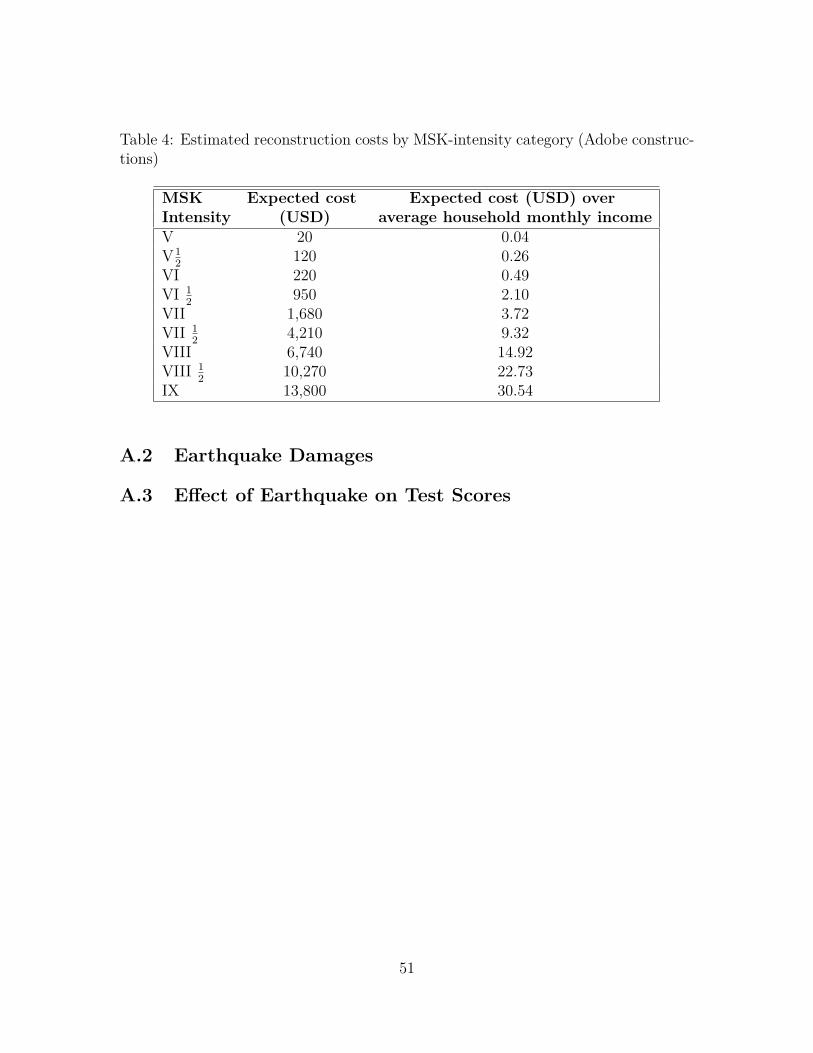
Table 4: Estimated reconstruction costs by MSK-intensity category (Adobe construc-tions)

MSK Expected cost Expected cost (USD) overIntensity (USD) average household monthly incomeV 20 0.04V1

2 120 0.26VI 220 0.49VI 1

2 950 2.10VII 1,680 3.72VII 1

2 4,210 9.32VIII 6,740 14.92VIII 1

2 10,270 22.73IX 13,800 30.54

A.2 Earthquake Damages

A.3 Effect of Earthquake on Test Scores

51

Figure 9: Typical damages to adobe structures and their corresponding grades ofdamage. (a) Vertical cracks at wall corner, G3; (b) diagonal crack in wall, G3; (c)wall collapse through out-of-plane, G4; (d) collapse of the roof, G5. Source: Thepicture and damage descriptions are reported from Astroza, Rui and Astroza (2012).

52

Tabl

e5:

Diff

eren

ce-in

-diff

eren

ces

eval

uatio

nof

eart

hqua

keim

pact

onte

stsc

ores

,de

pend

ent

varia

bles

Span

ishan

dM

athe

mat

ics

test

scor

esin

eigh

thgr

ade

Span

ishM

athe

mat

ics

(1)

(2)

(3)

(4)

(5)

(6)

(7)

(8)

Mun

icip

alVo

uche

rU

nsub

sidiz

edA

llSc

hool

sM

unic

ipal

Vouc

her

Uns

ubsid

ized

All

Scho

ols

Span

ishte

stsc

ore

0.65

6***

0.64

2***

0.59

5***

0.64

5***

info

urth

grad

e(0

.002

49)

(0.0

0240

)(0

.006

51)

(0.0

0167

)

Mat

hte

stsc

ore

0.63

5***

0.65

5***

0.64

6***

0.64

5***

info

urth

grad

e(0

.002

34)

(0.0

0231

)(0

.006

23)

(0.0

0159

)

Hou

seho

ld3.

61e-

08**

2.86

e-08

***

1.51

e-08

2.52

e-08

***

7.68

e-08

***

4.98

e-08

***

6.44

e-08

***

6.03

e-08

***

inco

me

(CLP

)(1

.10e

-08)

(6.3

8e-0

9)(9

.60e

-09)

(4.7

0e-0

9)(1

.03e

-08)

(5.9

1e-0

9)(8

.46e

-09)

(4.3

5e-0

9)

Fath

er’s

0.00

940*

**0.

0075

6***

0.01

37**

*0.

0088

5***

0.00

634*

**0.

0075

6***

0.01

15**

*0.

0071

5***

educ

atio

n(y

rs)

(0.0

0079

5)(0

.000

782)

(0.0

0208

)(0

.000

538)

(0.0

0074

1)(0

.000

724)

(0.0

0183

)(0

.000

497)

Mot

her’s

0.01

02**

*0.

0087

0***

0.01

33**

*0.

0098

2***

0.00

806*

**0.

0078

5***

0.01

62**

*0.

0085

9***

educ

atio

n(y

rs)

(0.0

0081

9)(0

.000

830)

(0.0

0191

)(0

.000

557)

(0.0

0076

5)(0

.000

768)

(0.0

0169

)(0

.000

516)

Fem

ale

0.13

4***

0.12

1***

0.10

1***

0.12

4***

-0.0

999*

**-0

.110

***

-0.0

880*

**-0

.104

***

(0.0

0439

)(0

.004

15)

(0.0

104)

(0.0

0290

)(0

.004

10)

(0.0

0385

)(0

.009

14)

(0.0

0268

)

Hou

seho

ldliv

es0.

0725

+0.

0431

0.06

530.

0566

*0.

110*

*0.

0063

6-0

.018

60.

0395

+in

eart

hqua

kere

gion

(E)

(0.0

417)

(0.0

337)

(0.0

766)

(0.0

247)

(0.0

390)

(0.0

313)

(0.0

677)

(0.0

229)

Coh

ort

2007

-201

1,0.

0529

***

0.05

79**

*0.

0469

+0.

0548

***

0.04

97**

*0.

0380

***

0.02

090.

0429

***

affec

ted

byea

rthq

uake

(P)

(0.0

0815

)(0

.008

64)

(0.0

271)

(0.0

0580

)(0

.007

55)

(0.0

0799

)(0

.023

8)(0

.005

35)

P*E

-0.0

377*

**-0

.044

0***

-0.1

15**

*-0

.049

2***

-0.0

284*

*-0

.063

3***

-0.0

519*

-0.0

509*

**(0

.009

69)

(0.0

0981

)(0

.029

1)(0

.006

67)

(0.0

0900

)(0

.009

08)

(0.0

256)

(0.0

0616

)

Con

stan

t-0

.429

***

-0.2

74**

*-0

.180

*-0

.333

***

-0.3

73**

*-0

.099

9***

0.05

26-0

.185

***

(0.0

309)

(0.0

283)

(0.0

769)

(0.0

200)

(0.0

288)

(0.0

263)

(0.0

679)

(0.0

185)

Scho

olFi

xed

Effec

tsye

sye

sye

sye

sye

sye

sye

sye

sO

bser

vatio

ns97

057

1164

4620

389

2338

9297

658

1170

1120

501

2351

70St

anda

rder

rors

inpa

rent

hese

s+p<

0.10

,*p<

0.05

,**p<

0.01

,***

p<

0.00

1

53

Table 6: Pre-Earthquake Cohort, dependent variables Spanish and Math test scoresin eighth grade

(1) (2)Spanish Math

Spanish test score in fourth grade 0.676***(0.00408)

Math test score in fourth grade 0.638***(0.00383)

Household income (CLP) 2.99e-08 9.66e-08***(1.82e-08) (1.73e-08)

Father’s education (yrs) 0.00874*** 0.00584***(0.00126) (0.00118)

Mother’s education (yrs) 0.00731*** 0.00559***(0.00130) (0.00122)

Female 0.138*** -0.109***(0.00715) (0.00674)

Own Intensity 0.0149 0.0146(0.0129) (0.0120)

Classroom Intensity 0.00943 0.0580Mean (0.0688) (0.0648)

Classroom Intensity 0.223+ 0.319**Variance (0.128) (0.120)

Constant -0.472 -0.681+(0.425) (0.400)

School Fixed Effects yes yesObservations 35175 35302Standard errors in parentheses+ p < 0.10, * p < 0.05, ** p < 0.01, *** p < 0.001Only municipal schools are in the estimation sample.

54

Table 7: Probit regression, marginal probability estimates reported. Dependent vari-ables: being a at top or bottom third of the distribution of elicited cost of effort

top 33 percent bottom 33 percent

Mother’s education .0007012 .0020148∗(.0007415 ) (.0008893)

Father’s education -.0007132 .0013843(.0007134) (.0008544)

Household income 1.76e− 08+ −2.32e− 08+

(1.02e-08) (1.23e-08)

Math test score t-1 −.0549353∗∗∗ .1004088∗∗∗(.0019868) (.0023838)

Seismic intensity .0128674∗∗∗ −.0105234∗∗∗at student’s home (.0022842) (.002741)Observations 46059 46059Standard errors in parentheses+ p < 0.10, * p < 0.05, ** p < 0.01, *** p < 0.001

55

A.4 Algorithm for the Estimation of the Semiparametric Single-Index Model

1. Normalize to a constant one of the elements of α1, because only the ratios amongthe components of α are identified. I normalize to -1 the coefficient on initialability (lagged test score).

2. Make an initial guess for all the other elements of α.

3. Form ci ∀i according to ci = α1xi if i belongs to the pre-earthquake cohort,and ci = α1xi + α2Ii + α3Iixi if i belongs to the post-earthquake cohort. Ii isinteracted with household income and student gender.

4. Estimate E(yi|c, l;α) ∀l by Nadaraya-Watson kernel regression with weights wi:

ml(c;α) =∑i∈l wiK

(ci−ch

)yi∑

i∈l wiK(ci−ch

)with a standard normal Kernel: K(ψ) = (2π)− 1

2 exp(−0.5ψ2) and optimal band-width h = 1.06σcn−1/5, minimizing the Approximated Mean Integrated SquaredError (AMISE).44 The weights wi are such that only observations i where thep.d.f. of c at ci exceeds a small positive number are used (see Ichimura (1993)and Horowitz (2010)). Observation i is excluded from the calculation of m atci.

5. Compute the sum of squared residuals in each l at the current guess for α:SSRl(α) = ∑

i∈l wi(yi − ml(ci;α))2. The weights are the same as those used inthe kernel estimator of m.

6. Update guess for α using Generating Set Search algorithm (HOPSPACK).

7. Repeat steps 1-6 until convergence to the minimizer of ∑l SSRl(α).

Notice that unlike in the standard semiparametric single-index model, here the SSR(α)is computed in each classroom l, and its sum over classrooms is minimized. The

44The MISE is equal to E{∫

[m(c)−m(c)]2dx} =∫ [

(Biasm)2 + V (m)]dc, and AMISE substitutes

the expressions for the bias and variance of m with approximations. See Pagan and Ullah (1999),p. 24.

56

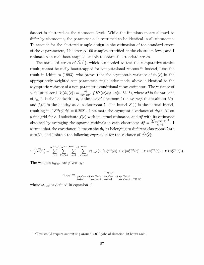
dataset is clustered at the classroom level. While the functions m are allowed todiffer by classrooms, the parameter α is restricted to be identical in all classrooms.To account for the clustered sample design in the estimation of the standard errorsof the α parameters, I bootstrap 100 samples stratified at the classroom level, and Iestimate α in each bootstrapped sample to obtain the standard errors.

The standard errors of ∆e(·), which are needed to test the comparative staticsresult, cannot be easily bootstrapped for computational reasons.45 Instead, I use theresult in Ichimura (1993), who proves that the asymptotic variance of ml(c) in theappropriately weighted semiparametric single-index model above is identical to theasymptotic variance of a non-parametric conditional mean estimator. The variance ofsuch estimator is V (ml(c)) = σ2

l

nlhlfl(c)∫K2(ψ)dψ+o(n−1h−1), where σ2 is the variance

of εil, hl is the bandwidth, nl is the size of classroom l (on average this is almost 30),and fl(c) is the density at c in classroom l. The kernel K(·) is the normal kernel,resulting in

∫K2(ψ)dψ = 0.2821. I estimate the asymptotic variance of ml(c) ∀l on

a fine grid for c. I substitute f(c) with its kernel estimator, and σ2l with its estimator

obtained by averaging the squared residuals in each classroom: σ2l =

∑i∈l(yi−yi)

2

nl−1 . Iassume that the covariances between the ml(c) belonging to different classrooms l arezero ∀c, and I obtain the following expression for the variance of ∆e(c):

V(

∆e(c))

=Npre−1∑l=1

Npre∑l′=l+1

Npost−1∑s=1

Npost∑s′=s+1

κ2ll′ss′

(V(mposts (c)

)+ V

(mposts′ (c)

)+ V (mpre

l (c)) + V (mprel′ (c))

).

The weights κll′ss′ are given by:

κll′ss′ = ωll′ss′∑Npre−1l=1

∑Npre

l′=l+1∑Npost−1s=1

∑Npost

s′=s+1 ωll′ss′

where ωll′ss′ is defined in equation 9.

45This would require submitting around 4,000 jobs of duration 72 hours each.

57

mprel

(c)

mpre

l′(c)

c0

G.D.E. ∆mpre

ll′(c)

c0

σ2Il− σ2

Il′ = ∆ > 0

mposts (c)

mpost

s′(c)

c0

G.D.E.+P.E.

∆mpost

ss′(c)

c0

σ2Is − σ

2Is′ = ∆ > 0

Figure 10: Classrooms l, l′ , s, and s′ are identical in terms of classroom and student

characteristics. G.D.E. is the effect of geographic dispersion, P.E. is the peer effect ofinterest.

A.5 Differencing technique

58

G.D.E.+P.E.G.D.E.∆mpre

ll′(c)

∆mpost

ss′(c)

c0

P.E.

∆mpost(c)−∆mpre(c)

c0

Figure 11: Differencing out the geographic dispersion effects. Notice that the differ-ence between the ∆mpost and ∆mpre functions can be taken only over the overlappingportion of the two domains. The domain of ∆mpost is shifted to the right with respectto the domain of ∆mpre, because all students have been affected by the earthquakeand, therefore, their cost of effort is larger than for pre-earthquake students.

59

Intuitively, for the kernel weighting method and dimensionality reduction to de-liver the desired result, two sets of conditions must be met. First, ψl(·) and ul(·)must vary smoothly with zl, Fl(xi), Il, Il. This guarantees that there are no jumps inthese functions when two classrooms that are similar, but not identical, in these vari-ables are compared. Similarly, when two classrooms are similar but not identical inthese variables, the distributions of c are similar but not identical. To avoid jumps inthe e(c;Gl(c)) function, one needs to assume that this function varies smoothly withGl(c).46 Second, it must be innocuous to consider only a finite number of momentsrather than the entire distribution of student characteristics. Formally, I make thefollowing additional assumptions:DA.1 u(ci, zl, Fl(xi), Il, Il, σ2

Il) and ψ(ci, zl, Fl(xi), Il, Il, σ2Il) are continuous in zl, Fl(xi), Il, Il.

DA.2 φ(ci, zl, Fl(xi), Il, Il, σ2Il) (where φ(·) = u(·)+ψ(·)) is similar to φ(ci, zl,Wl, Il, Il, σ

2Il)

∀(c, zl,Wl, σ2Il), where Wl is a vector containing the mean, variance, skewness and

kurtosis of the elements of xi.47.DA.3 φ(·) is continuous in zl, Il, Il and Wl.DA.4 If two classrooms in the pre-earthquake cohort are such that Wl ∼= Wl′ , thenel(c) ∼= el′(c) ∀c. If two classrooms in the post-earthquake cohort are such that[Ws, Is, Is, σ

2Is] ∼= [Ws′ , Is′ , Is′ , σ

2Is′ ], then es(c) ∼= es′(c) ∀c.

These assumptions allow me to build an approximated counterpart to equation 6.Assumption DA.1 implies that if two classrooms are similar, then the classroom effectsare also similar for every student type c. Assumptions DA.2 and DA.3 together meanthat if two classrooms are similar, then φ(ci, zl,Wl, Il, Il, σ

2Il)−φ(ci, zl′ ,Wl′ , Il′ , Il′ , σ

2Il′) ∼=

∆φll′(c). That is, the difference between the φ functions computed in classrooms withsimilar vectors W and z is a good approximation to the spurious effect in equations4 and 5. Finally, assumption DA.4 means that when the distribution of c varies in aclassroom, if this affects el(c) because there are peer effects, then el(c) varies smoothlywith the change in the distribution of c. As a result of these four assumptions, for anytwo classrooms l, l′ in the pre-earthquake cohort with Wl ∼= Wl′ , zl ∼= zl′ , Il ∼= Il′ ,Il ∼= Il′ and σ2

Il − σ2Il′ = ∆σ2

Ill′ < 0, I can build the approximated counterpart to∆mpre

ll′ (c), ∆mprell′ (c). Similarly, for two similar classrooms in the post-earthquake

cohort, I can build the approximated counterpart to ∆mpostss′ (c), ∆mpost

ss′ (c). If four46In Ahn and Powell (1993), this assumption corresponds to continuity of the selection function

(see page 9 in their paper).47I ignore the cross-moments of xi to make the numerical implementation tractable.

60

classrooms, l, l′ from the pre-earthquake cohort and s, s′ from the post-earthquakecohort, are such that Wl ∼= Wl′ ∼= Ws ∼= Ws′ , zl ∼= zl′ ∼= zs ∼= zs′ , Il ∼= Il′ ∼= Is ∼= Is′ ,Il ∼= Il′ ∼= Is ∼= Is′ and 0 > ∆σ2

Ill′∼= ∆σ2

Iss′ < 0, then subtracting ∆mprell′ (c) from

∆mpostll′ (c) yields an approximation to ∆ess′(c) + ∆ξill′ss′ , the quantity of interest.To ensure that the classrooms are similar, I assign increasing weights to quadruples

that are more similar in terms of W, z, I, I and ∆σ2I . I construct weights using mul-

tivariate standard normal kernel functions. As before, let ll′ index a pre-earthquakeclassroom pair, and ss′ a post-earthquake classroom pair. Letting Zt = [Wt, zt, It, It]for t = l, l′, s, s′, I assign the weight 1

hk(Zt−Zt′

h

)to each of the pairs tt′ ∈ {ll′, ss′, sl}.

This ensures that the pairs within the pre- and post-earthquake cohorts are composedof classrooms that are similar to each other in terms of W and z (tt′ = ll′, ss′), andalso that across cohorts the two pairs of classrooms are similar (tt′ = sl).48 Finally,I build a weight that is declining in |∆σ2

Ill′ −∆σ2Iss′|, to guarantee that the pre- and

post-earthquake pairs differ in terms of σ2I in a similar way, i.e., that the intensities of

treatment in the two pairs of classrooms are very similar: 1h∆σ

k(

∆σ2Ill′−∆σ2

Iss′h

). The

weight for the quadruple, ωll′ss′ , is the product of these four kernel weights:

ωll′ss′ = dll′ss′1h∆σ

k

(∆σ2

Ill′ −∆σ2Iss′

h

) ∏tt′∈{ll′,ss′,sl}

1hk(Zt − Zt′

h

)(9)

where dll′ss′ is a dummy variable equal to one if ∆σ2Ill′ < 0 and ∆σ2

Iss′ < 0. Foreach value of c, the estimator of ∆ess′(c) is obtained by estimating γ in the followingweighted regression on a constant:

( ∆mpostss′ − ∆mpre

ll′ ) = ωll′ss′γ + ξll′ss′

with E[ξll′ss′ ] = 0. The OLS estimator of γ is the following weighted sample mean:

γ = ∆e(c) =∑Npre−1l=1

∑Npre

l′=l+1∑Npost−1s=1

∑Npost

s′=s+1 ωll′ss′(∆mpostss′ (c)− ∆mpre

ll′ (c))∑Npre−1l=1

∑Npre

l′=l+1∑Npost−1s=1

∑Npost

s′=s+1 ωll′ss′. (10)

The parameter γ computed at a value for c yields the value of the ∆e(·) function atone point. Estimating γ over a grid of values for c allows me to trace the behavior of

48Notice that I use a unique bandwidth. Following Pagan and Ullah (1999), I normalize thevariables Zt so that they all have the same standard deviation, and using a unique bandwidth isadmissible.

61

this function over its domain, and to detect how the effects of changing the varianceof student types (peer effects) vary across student types. Computing γ at each gridpoint requires doing a number of calculations of the order of 1012, therefore, parallelprocessing is required.

A.6 Identifying Assumption

62

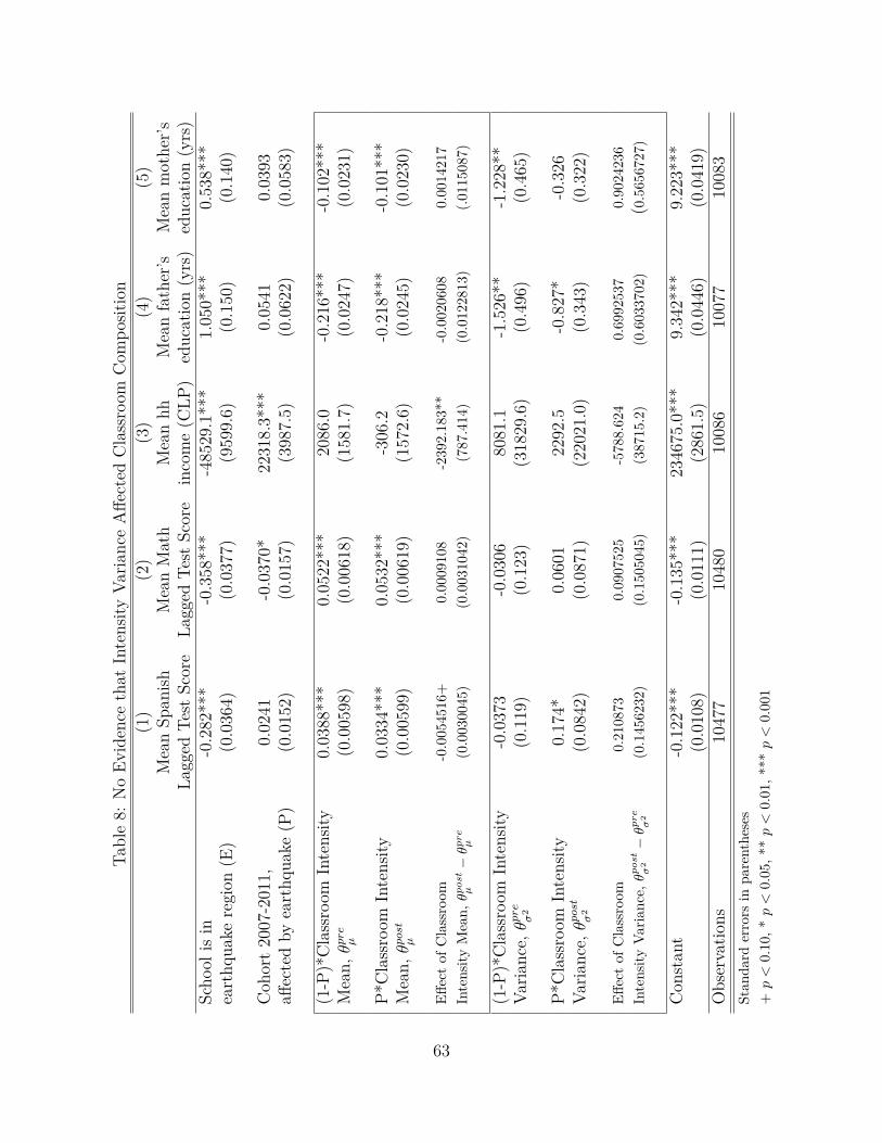
Tabl

e8:

No

Evid

ence

that

Inte

nsity

Varia

nce

Affe

cted

Cla

ssro

omC

ompo

sitio

n(1

)(2

)(3

)(4

)(5

)M

ean

Span

ishM

ean

Mat

hM

ean

hhM

ean

fath

er’s

Mea

nm

othe

r’sLa

gged

Test

Scor

eLa

gged

Test

Scor

ein

com

e(C

LP)

educ

atio

n(y

rs)

educ

atio

n(y

rs)

Scho

olis

in-0

.282

***

-0.3

58**

*-4

8529

.1**

*1.

050*

**0.

538*

**ea

rthq

uake

regi

on(E

)(0

.036

4)(0

.037

7)(9

599.

6)(0

.150

)(0

.140

)

Coh

ort

2007

-201

1,0.

0241

-0.0

370*

2231

8.3*

**0.

0541

0.03

93aff

ecte

dby

eart

hqua

ke(P

)(0

.015

2)(0

.015

7)(3

987.

5)(0

.062

2)(0

.058

3)

(1-P

)*C

lass

room

Inte

nsity

0.03

88**

*0.

0522

***

2086

.0-0

.216

***

-0.1

02**

*M

ean,θpre

µ(0

.005

98)

(0.0

0618

)(1

581.

7)(0

.024

7)(0

.023

1)

P*C

lass

room

Inte

nsity

0.03

34**

*0.

0532

***

-306

.2-0

.218

***

-0.1

01**

*M

ean,θpost

µ(0

.005

99)

(0.0

0619

)(1

572.

6)(0

.024

5)(0

.023

0)

Effec

tof

Cla

ssro

om-0

.005

4516

+0.

0009

108

-239

2.18

3**

-0.0

0206

080.

0014

217

Inte

nsity

Mea

n,θpost

µ−θpre

µ(0

.003

0045

)(0

.003

1042

)(7

87.4

14)

(0.0

1228

13)

(.011

5087

)

(1-P

)*C

lass

room

Inte

nsity

-0.0

373

-0.0

306

8081

.1-1

.526

**-1

.228

**Va

rianc

e,θpre

σ2

(0.1

19)

(0.1

23)

(318

29.6

)(0

.496

)(0

.465

)

P*C

lass

room

Inte

nsity

0.17

4*0.

0601

2292

.5-0

.827

*-0

.326

Varia

nce,θpost

σ2

(0.0

842)

(0.0

871)

(220

21.0

)(0

.343

)(0

.322

)

Effec

tof

Cla

ssro

om0.

2108

730.

0907

525

-578

8.62

40.

6992

537

0.90

2423

6In

tens

ityVa

rianc

e,θpost

σ2−θpre

σ2

(0.1

4562

32)

(0.1

5050

45)

(387

15.2

)(0

.603

3702

)(0

.565

6727

)

Con

stan

t-0

.122

***

-0.1

35**

*23

4675

.0**

*9.

342*

**9.

223*

**(0

.010

8)(0

.011

1)(2

861.

5)(0

.044

6)(0

.041

9)O

bser

vatio

ns10

477

1048

010

086

1007

710

083

Stan

dard

erro

rsin

pare

nthe

ses

+p<

0.10

,*p<

0.05

,**p<

0.01

,***

p<

0.00

1

63

Tabl

e9:

No

Evid

ence

that

the

Rel

atio

nshi

pBe

twee

nC

lass

room

Inte

nsity

Varia

nce

and

Cla

ssro

omQ

ualit

yC

hang

edA

fter

the

Eart

hqua

keSt

ruck

(Spa

nish

teac

hers

)(1

)(2

)(3

)(4

)(5

)Sp

anish

Teac

her

Cla

ssPe

rman

ent

Expe

rienc

ePo

stgr

adFe

mal

esiz

eco

ntra

ctde

gree

Scho

olis

inea

rthq

uake

1.78

4+0.

137

0.27

30.

0761

-0.3

44**

regi

on(E

)(0

.913

)(0

.114

)(1

.247

)(0

.113

)(0

.129

)C

ohor

t20

07-2

011,

affec

ted

-2.2

69**

*0.

203*

**-0

.536

0.33

6***

0.05

60by

eart

hqua

ke(P

)(0

.381

)(0

.048

2)(0

.547

)(0

.047

8)(0

.056

5)(1

-P)*

Cla

ssro

omIn

tens

ity-0

.278

+-0

.005

8-0

.121

0.02

970.

0666

**M

ean,θpre

µ(0

.150

)(0

.018

8)(0

.207

)(0

.018

7)(0

.021

4)P*

Cla

ssro

omIn

tens

ity-0

.324

*-0

.030

9+-0

.105

0.00

940.

0697

**M

ean,θpost

µ(0

.150

)(0

.018

6)(0

.204

)(0

.018

5)(0

.021

2)Eff

ect

ofC

lass

room

Inte

nsity

-0.0

457

-0.0

252*

*0.

0162

-0.0

203*

0.00

31M

ean,θpost

µ−θpre

µ(0

.074

9)(0

.009

5)(0

.106

5)(0

.009

4)(0

.011

1)(1

-P)*

Cla

ssro

omIn

tens

ity-7

.374

*-0

.240

-5.6

530.

585

-0.3

31Va

rianc

e,θpre

σ2

(2.9

36)

(0.3

74)

(4.1

21)

(0.4

00)

(0.4

16)

P*C

lass

room

Inte

nsity

-9.2

18**

*0.

0429

1.25

5-0

.105

-0.3

79Va

rianc

e,θpost

σ2

(2.0

95)

(0.2

75)

(2.8

67)

(0.2

66)

(0.2

83)

Effec

tof

Cla

ssro

omIn

tens

ity-1

.843

70.

2832

6.90

77-0

.690

14-0

.047

6Va

rianc

e,θpost

σ2−θpre

σ2

(3.6

082)

(0.4

645)

(5.0

200)

(0.4

807)

(0.5

037)

Con

stan

t25

.60*

**0.

139*

*22

.38*

**-0

.146

**0.

780*

**(0

.381

)(0

.048

7)(0

.563

)(0

.048

5)(0

.057

6)O

bser

vatio

ns10

339

9128

8358

9128

8529

Stan

dard

erro

rsin

pare

nthe

ses

+p<

0.10

,*p<

0.05

,**p<

0.01

,***

p<

0.00

1

64

Tabl

e10

:N

oEv

iden

ceth

atth

eR

elat

ions

hip

Betw

een

Cla

ssro

omIn

tens

ityVa

rianc

ean

dC

lass

room

Qua

lity

Cha

nged

Afte

rth

eEa

rthq

uake

Stru

ck(M

ath

Teac

hers

)(6

)(7

)(8

)(9

)M

ath

Teac

her

Perm

anen

tEx

perie

nce

Post

grad

Fem

ale

Con

trac

tde

gree

Scho

olis

inea

rthq

uake

0.17

11.

307

-0.3

19**

-0.0

557

regi

on(E

)(0

.113

)(1

.230

)(0

.113

)(0

.114

)C

ohor

t20

07-2

011,

affec

ted

0.26

5***

0.32

90.

307*

**0.

0398

byea

rthq

uake

(P)

(0.0

482)

(0.5

43)

(0.0

476)

(0.0

502)

(1-P

)*C

lass

room

Inte

nsity

-0.0

045

-0.2

490.

0847

***

0.02

67M

ean,θpre

µ(0

.018

7)(0

.204

)(0

.018

7)(0

.018

8)P*

Cla

ssro

omIn

tens

ity-0

.042

0*-0

.415

*0.

0735

***

0.01

46M

ean,θpost

µ(0

.018

5)(0

.201

)(0

.018

6)(0

.018

6)Eff

ect

ofC

lass

room

Inte

nsity

- 0.03

75**

*-0

.165

5-0

.011

2-0

.012

1

Mea

n,θpost

µ−θpre

µ(0

.009

4)(0

.105

3)(0

.009

4)(0

.009

7)(1

-P)*

Cla

ssro

omIn

tens

ity-0

.425

-7.5

41+

0.74

3+-0

.574

Varia

nce,θpre

σ2

(0.3

70)

(4.1

00)

(0.4

19)

(0.3

78)

P*C

lass

room

Inte

nsity

-0.1

42-0

.170

0.22

0-0

.122

Varia

nce,θpost

σ2

(0.2

61)

(2.7

50)

(0.2

59)

(0.2

57)

Effec

tof

Cla

ssro

omIn

tens

ity0.

2826

7.37

15-0

.523

10.

4523

Varia

nce,θpost

σ2−θpre

σ2

(0.4

529)

(4.9

383)

(0.4

925)

(0.4

573)

Con

stan

t0.

224*

**23

.25*

**-0

.061

10.

0621

(0.0

484)

(0.5

52)

(0.0

480)

(0.0

511)

Obs

erva

tions

9229

8508

9229

8623

Stan

dard

erro

rsin

pare

nthe

ses

+p<

0.10

,*p<

0.05

,**p<

0.01

,***

p<

0.00

1

65

A.7 Testing Monotonicity of m(c)

The procedure that I use is an application of Chetverikov (2013). It would be com-putationally unfeasible to perform the test in all classrooms. Therefore, I create 72categories of classrooms that have similar distributions of c, and test monotonic-ity within each category. Consider classroom categories containing approximately 60classrooms each. Classrooms in the same category share similar mean and variance ofc. Therefore, the theoretical model predicts that the equilibrium e functions shouldbe very similar across classrooms within each category. The monotonicity of m istested within each one of these categories. Separating the sample in categories makesthis procedure feasible from a computational point of view. In all categories, thenull hypothesis that the m function is decreasing is not rejected at the α = 0.10significance level.

Details of the simulations can be found in the Online Supplementary Material onthe author’s webpage. I follow the choice of bandwidth recommended in Ghosal, Sen,and Van Der Vaart (2000), and I adopt the plug-in approach to simulate the criticalvalues.

An important distinction with Chetverikov (2013) is that the ci values in mysample are estimated (and not observed); ci = α1xi + α2IiPi + α3IiPixi. However,this additional noise is asymptotically negligible because the bandwidth used in thekernel weighting functions goes to zero as the sample size increases, and because αis root-n consistent (as shown in Ichimura (1993)), therefore, it is faster than thenonparametric rates appearing in the derivations in Chetverikov (2013).

A.8 Robustness

66

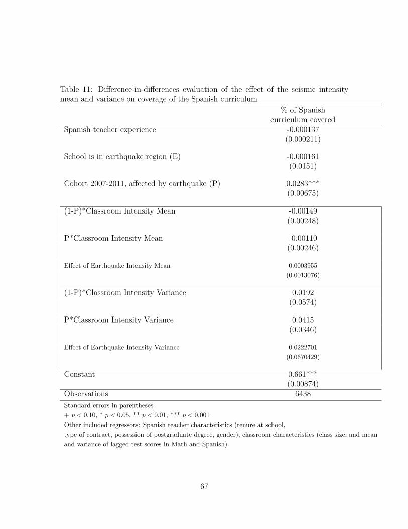
Table 11: Difference-in-differences evaluation of the effect of the seismic intensitymean and variance on coverage of the Spanish curriculum

% of Spanishcurriculum covered

Spanish teacher experience -0.000137(0.000211)

School is in earthquake region (E) -0.000161(0.0151)

Cohort 2007-2011, affected by earthquake (P) 0.0283***(0.00675)

(1-P)*Classroom Intensity Mean -0.00149(0.00248)

P*Classroom Intensity Mean -0.00110(0.00246)

Effect of Earthquake Intensity Mean 0.0003955(0.0013076)

(1-P)*Classroom Intensity Variance 0.0192(0.0574)

P*Classroom Intensity Variance 0.0415(0.0346)

Effect of Earthquake Intensity Variance 0.0222701(0.0670429)

Constant 0.661***(0.00874)

Observations 6438Standard errors in parentheses+ p < 0.10, * p < 0.05, ** p < 0.01, *** p < 0.001Other included regressors: Spanish teacher characteristics (tenure at school,type of contract, possession of postgraduate degree, gender), classroom characteristics (class size, and meanand variance of lagged test scores in Math and Spanish).

67

Table 12: Difference-in-Differences Evaluation of the Effect of Seismic Intensity Vari-ance on Test Scores. Dependent variables Spanish and Math test scores in eighthgrade.

(1) (2)Math Spanish

Math test score in 4th 0.638***grade (0.00254)

Spanish test score in 4th 0.657***grade (0.00272)[1em] Household lives 0.338* 0.0874in earthquake region (E) (0.133) (0.143)

Cohort 2007-2011, affected 0.0371*** 0.0528***by the earthquake (P) (0.00936) (0.00997)

(1-P)*Classroom 0.0753 -0.193+Intensity Mean (0.102) (0.111)

P*Classroom 0.0676 -0.191+Intensity Mean (0.102) (0.111)

Effect of -0.0076943 0.0020984Intensity Mean (0.0158669) (0.0169411)

(1-P)*Classroom -0.113 0.238*Intensity Variance (0.101) (0.108)

P*Classroom -0.0243 -0.0171Intensity Variance (0.0633) (0.0719)

Effect of 0.0885604 −0.2549768∗

Intensity Variance (0.1149763) (0.124782)

Constant -0.675 0.331(0.449) (0.484)

Observations 83295 81307Standard errors in parentheses+ p < 0.10, * p < 0.05, ** p < 0.01, *** p < 0.001Other included regressors: household income, seismic intensity at home interacted with cohort dummy,father’s education, mother’s education, student gender, teacher gender, teacher experience, class size.

68