"Portfolio Optimisation When You Don’t Know the Future (or the Past)" by Rob Carver, Independent Systematic Futures Trader, Writer and Research Consultant

Portfolio optimisation when you don’t know

the future(or the past)

Robert Carver

QuantCon, Singapore29th September 2017

Legal boilerplate bit:

Nothing in this presentation constitutes investment advice, or an offer or solicitation to conduct investment business. The material here is solely for educational purposes.

I am not currently regulated or authorised by the FCA, SEC, CFTC, MAS, or any other regulatory body to give investment advice, or indeed to do anything else.

Futures trading carries significant risks and is not suitable for all investors. Back tested and actual historic results are no guarantee of future performance. Use of the material in this presentation is entirely at your own risk.

● Two nightmares: Instability and Uncertainty● The uncertainty of the past● Common solutions● Alternatives


Instability

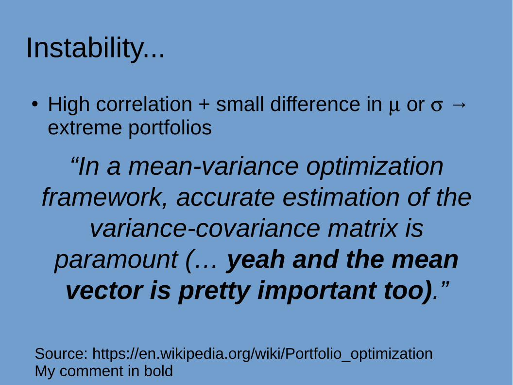
Instability...

● High correlation + small difference in or → extreme portfolios

“In a mean-variance optimization framework, accurate estimation of the

variance-covariance matrix is paramount (… yeah and the mean vector is pretty important too).”

Source: https://en.wikipedia.org/wiki/Portfolio_optimization My comment in bold

Uncertainty

● Can we measure or accurately?● NO● We can’t predict the future – must assume the

past will repeat itself● Need to fit a statistical model to historic returns

(e.g. estimate and )

Need to fit a statistical model:

● Do we have the right model?– Can use more complex models, with higher moments. Hard to

estimate. Markowitz optimisation built for Gaussian returns – hard to change. Correct utility preferences?

● Will the model change?– Could try Markov process. Many more parameters to estimate

(Given K states, KN+[K-1]2). Overlap with historical parameter estimates.

● Do we have accurate historical parameter estimates?– Easy to quantify. Can capture changes in model. Worth exploring…

“The Uncertainty of the Past”


SP500 US10 US5

Return 0% 4.1% 3.1%

Std. dev 18.7% 7.1% 4.7%

Sharpe ratio 0.0 0.59 0.66

SP500/US5 SP500/US10 US5/US10

Correlation -0.28 -0.27 0.96

Based on weekly excess returns (futures, including rolldown) from 01/1998 to 11/2016

SP500 US10 US5

Weight 12.9% 0% 87.1%

Bootstrapped Correlations

10,000 monte carlo draws with replacement; same length as data history

Bootstrapped standard deviation


Bootstrapped means


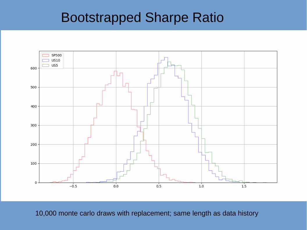
Bootstrapped Sharpe Ratio


Estimates get better with more data...

Upper 90%, Lower 10%, quantile of distribution of annualised standard deviation of US 5 year

… up to a point...

Upper 90%, Lower 10%, quantile of distribution of correlation of US 5 year and S&P 500

… which for Sharpe Ratios isn’t a very good point

Upper 90%, Lower 10%, quantile of distribution of annualised Sharpe Ratio of US 5 year

Mean SP500 US10 US5

Lower -5.7% 2.0% 1.7%

Upper 5.6% 6.3% 4.6%

Correlation SP500/US5

SP500/US10

US10/US5

Lower -0.33 -0.34 0.95

Upper -0.23 -0.21 0.97

Std dev SP500 US10 US5

Lower 17.3% 6.4% 4.2%

Upper 20.1% 7.8% 5.3%

Sharpe SP500 US10 US5

Lower -0.29 0.28 0.35

Upper 0.28 0.90 0.99

Lower: 10th percentile of bootstrapped distribution, Upper: 90th percentile

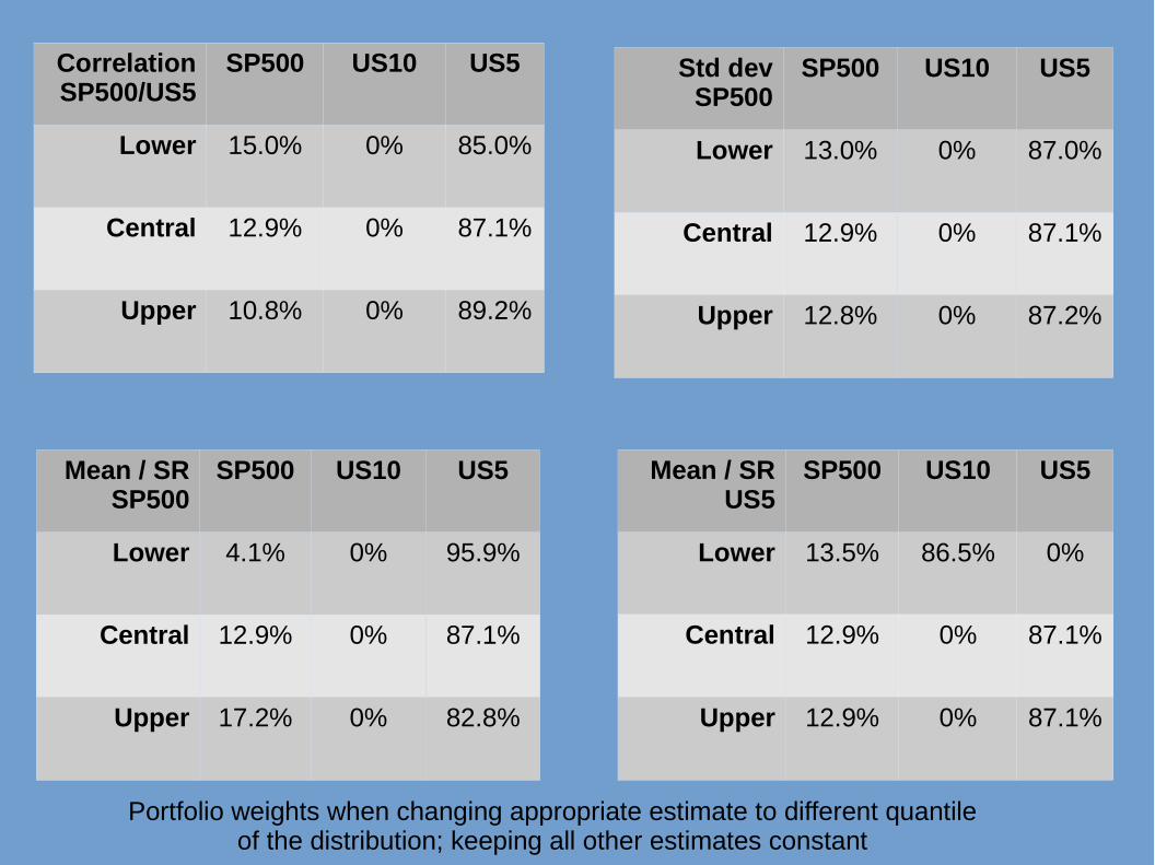
Correlation SP500/US5

SP500 US10 US5

Lower 15.0% 0% 85.0%

Central 12.9% 0% 87.1%

Upper 10.8% 0% 89.2%

Std dev SP500

SP500 US10 US5

Lower 13.0% 0% 87.0%

Central 12.9% 0% 87.1%

Upper 12.8% 0% 87.2%

Mean / SR SP500

SP500 US10 US5

Lower 4.1% 0% 95.9%

Central 12.9% 0% 87.1%

Upper 17.2% 0% 82.8%

Mean / SR US5

SP500 US10 US5

Lower 13.5% 86.5% 0%

Central 12.9% 0% 87.1%

Upper 12.9% 0% 87.1%

Portfolio weights when changing appropriate estimate to different quantile of the distribution; keeping all other estimates constant

● Land of low correlations:– Eg Asset classes (also different vol)– Relatively benign results – Almost impossible to distinguish historically estimated Sharpe Ratios

● Land of high correlations:– Eg Stocks in the same country (also similar vol)– Trading rules with same algo, different parameters– Extreme results– Theoretically possible to distinguish estimated Sharpe Ratios: but

similar assets more likely to have similar performance.

Years before we get 95% confidence in a mano et mano comparision...

Costs….

● Uncertainty of Sharpe Ratio mostly comes from returns…

● Uncertainty of post-cost returns mostly comes from pre-cost returns…

● Costs can be estimated with relatively high accuracy…– Caveat: Large size – Illiquid markets - High frequency trading

● Differential in costs should be treated differently to differential in pre-cost returns


Common Solutions...

● Constraints eg minimum and maximum weights● Ignore (some) estimated values eg assume

identical means● Change the inputs (bayesian) to reflect

uncertainty● Repeat the optimisation (bootstrapping)

Ignore some values

Correlation Sharpe SP500 US10 US5

Est Est 12.9% 0% 87.1%

Est Eq 20.2% 0% 79.8%

Eq Est 0% 37.0% 63.0%

Eq Eq 13.2% 34.8% 52.0%

Bayesian

Average between estimates and a prior

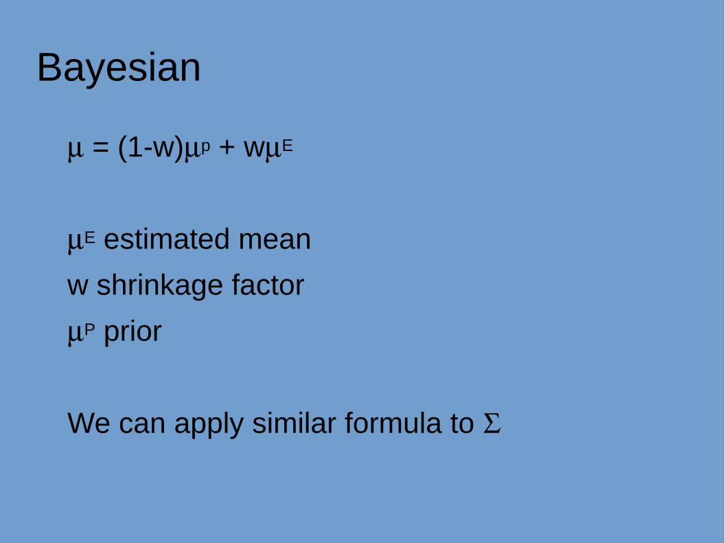
Bayesian

= (1-w)p + wE

E estimated mean

w shrinkage factor

P prior

We can apply similar formula to

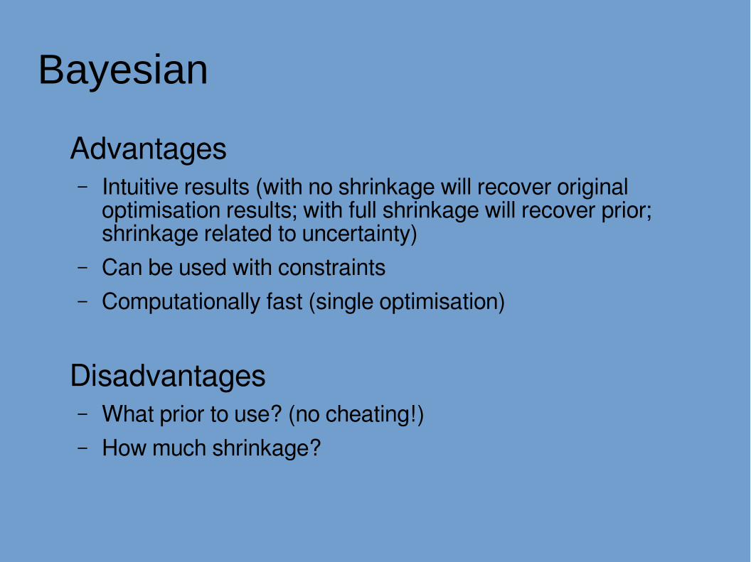
Bayesian

Advantages– Intuitive results (with no shrinkage will recover original

optimisation results; with full shrinkage will recover prior; shrinkage related to uncertainty)

– Can be used with constraints– Computationally fast (single optimisation)

Disadvantages– What prior to use? (no cheating!)– How much shrinkage?

Bayesian – Black Litterman style

Take estimated Take some prior weights wp

Infer p

= (1-w)p + wE

Bayesian – Black litterman styleAdvantages– Intuitive results (with full shrinkage will recover prior weights, with

none will recover original optimisation results)– Don’t have to come up with priors for or .– Focus Bayesian weapon on highest priority target:

Disadvantages– What prior weights to use? (market cap, heuristic cluster, equal

weights...)– How much shrinkage on mean?– No shrinkage on correlations or standard deviations – but still

uncertainty– Constraints aren’t used on the first, inverse, optimisation – prior

weights have to be feasible or results will be distorted

Bootstrapping

● Non parametric: Repeat optimisation using random subsets of data with replacement, take average of weights

● Parameteric: Repeat optimisation using random draws from fitted distribution, take average of weights. Good with small samples. Bad for non Gaussian (joint) returns.

● Michaud parametric: Repeat optimisation to create efficient frontier, take average of efficient frontiers.

Bootstrapping

Advantages:– Intuitive results depending on amount of uncertainty in data

(noise, horizon length)– Can be combined with other methods

Disadvantages– Final weights not intuitive in comparision to eg Bayesian– Results can sometimes be unsatisfactory, especially with high

correlations– Computationally intensive (especially rolling out of sample)– Inefficient use of constraints

● Two nightmares: Instability and Uncertainty● The uncertainty of the past● Boostrapping vs Shrinkage● Alternatives

Alternatives:

● Risk weighting● Clustering● Heuristic methods● Alternatives to portfolio construction:

– Fama-French factor sort (long / short baskets)– Parametric portfolio policy [weights = f(factors)]

Can combine these, and ‘traditional’ methods.

Risk weighting

● Produce weights assume equal volatility, then scale weights accordingly.

● Good for:– Produces a more stable optimisation

– Volatility estimate is seperated (can account for differential noise, and use other inputs eg implied vol, and account for vol tail risk)

● Bad:– Investors without leverage, and with high risk appetite, and with low volatility

assets (asset allocation problems)

● Commonly used by CTAs– Use to determine risk weighting of investment strategies, not optimise positions

Risk weighting + Optimisation

SP500 US10 US5

Risk weight 21.8% 0% 78.1%

Std. dev 18.7% 7.1% 4.7%

Cash weight (estimated)

2.67 3.52 5.32

Final cash weight 6.6% 0.0% 93.4%

Standard deviation: 4.2%Mean: 2.3% (assuming all assets have SR 0.4)Assumed mean of all stock portfolio: 7.5%→ avoid low volatility assets in portfolio if possible→ add constraints on lower vol assets

Risk weighting + ignore estimate(s)

Equalise Sharpe SP500 US10 US5

Risk weight 49.7% 21.1% 29.2%

Std. dev 18.7% 7.1% 4.7%


2.65 2.97 6.21



Equalise Correlations

SP500 US10 US5

Risk weight 0% 46.8% 53.2%

Std. dev 18.7% 7.1% 4.7%


0 6.59 11.3

Final cash weight 0% 36.8% 63.2%


Equalise Correlations & SR

SP500 US10 US5

Risk weight 33.3% 33.3% 33.3%

Std. dev 18.7% 7.1% 4.7%


1.8 4.7 7.1


Bayesian with risk weighting

= (1-w)p + wE

E estimated Sharpe ratio

w shrinkage factor

P prior Sharpe Ratio

We can apply similar formula to correlations,

Risk weighting plus Bayesian

Corr->SR

0.0 0.25 0.5 0.75 1.0

0.0 0.21, 0, 0.78 0.08, 0.11, 0.81 0, 0.3, 0.7 0, 0.37, 0.63 0, 0.4, 0.6

0.25 0.28, 0, 0.72 0.16, 0.14, 0.7 0, 0.32, 0.68 0, 0.38, 0.62 0, 0.42, 0.58

0.5 0.34, 0, 0.66 0.26, 0.17, 0.57 0.12, 0.31, 0.57 0, 0.4, 0.6 0, 0.43, 0.57

0.75 0.41, 0.0, 0.59 0.36, 0.21, 0.43 0.28, 0.29, 0.43 0.13, 0.38, 0.48 0, 0.47, 0.53

1.0 0.5, 0.25, 0.26 0.48, 0.26, 0.26 0.46, 0.27, 0.27 0.42, 0.29, 0.29 0.33, 0.33, 0.33


● Need high degree of shrinkage on SR to get non zero weights → we don’t know much about SR

● Too much shrinkage on correlation destroys information

● Precise optimal shrinkage depend on amount of data available. Can use fake data + monte carlo / closed form to derive optimal shrinkage.

● Rule of thumb: 0.95 on SR, 0.5 on correlations● Optimal shrinkage is context specific.


SR shrinkage 0.95 (prior SR 0.25), correlation 0.5 (prior correlation matrix, off diagonal 0.5)

Bayesian with risk weighting – Black Litterman style

Take estimated Take some prior weights wp

Infer Sharpe Ratio p

= (1-w)p + wE

Bootstrapping with risk weights

Bootstrapping with risk weights & identical SR

Clustering

● Group assets together into groups● Create sets of portfolios that are more tractable● Clustering can be formal (eg k-means) or heuristic

(‘handcrafting’)● Clustering can work on multiple levels● Optimisation within groups can be:

– Equal Weights (in risk weighting space)– Fully optimised

– Heuristic optimisation

Clustering: equal risk weight

Group Intra group weight

Group weight Risk Weight

S&P 500 Equity 100% 50% 50%

US 5 year Bonds 50%

50%

25%

US 10 year Bonds 50% 25%

SP500 US10 US5

Risk weight 50% 25% 25%

Std. dev 18.7% 7.1% 4.7%


2.67 3.52 5.32


Clustering: equal risk weight

Heuristic methods

● Miimicks what (experienced) people do when hand optimising – high comfort level

● Should be informed by theory / experiement● Sometimes hard to backtest - be careful of

implicit in sample fitting– I use other methods to backtest my system, but then use

heuristic weights in live trading.

● Suitable for ‘one off’ exercises, eg strategy risk allocation.

Heuristic methods

● Hueristic grouping when clustering● Equal weight within groups● Use ‘rule of thumb’ correlations, not estimates● Heuristic optimisation using correlations● Heruistic adjustment for different Sharpe Ratios

– Can apply different heuristic for pre-cost, and costs

● Use ‘rule of thumb’ risk levels, not estimates● Heuristic risk levels (constant risk, or assume equal)

Heuristic method for correlations in clustered groups (risk weightings)

Group of one asset100% to that asset

Any group of two assets 50% to each asset

Any size group with identical correlations Equal weights

Four or more assets without identical correlations Split groups further or differently until they match another row

Three assets with correlations AB, AC, BC: Weights for A, B, C

3 assets correlation 0.0, 0.5, 0.0 Weights: 30%, 40%, 30%







Correction for heterogenous groups

Given N assets with a correlation matrix of returns H and risk weights W summing to 1, the diversification multiplier will be:

1 / [ ( W x H x WT )1/2 ]

1) Calculate diversification multiplier for each group

2) Multiply group weight by multiplier

3) Renormalise group weights to add up to 100%

4) Apply at all levels of a hierarchy

Correction for heterogenous groups

SP500 US10 US5

Start Risk weight 50% 25% 25%

Diversification multiplier 1 1.01015 1.01015

Adjusted risk weight 50% 25.3% 25.3%

Normalised risk weight 49.7% 25.1% 25.1%

Heuristic correction for relative Sharpe Ratios

-0.5 -0.4 -0.3 -0.25 -0.2 -0.15 -0.1 -0.05 0 0.05 0.1 0.15 0.2 0.25 0.3 0.4 0.50

0.5

1

1.5

2

2.5

(A) With certainty eg costs

(B) Without certainty, more than ten years data

rule of thumb

Heuristic correction for relative Sharpe Ratios

SP500 US10 US5

Start risk weight 50% 25% 25%Sharpe Ratio 0.0 0.59 0.66

Adjustment 0.75 1.11 1.15Multiplied risk

weight37.5% 27.8% 28.8%

Normalised risk weight

40% 29.5% 30.5

Conclusions...

● Be aware of uncertainty!● Uncertainty in Sharpe Ratios is bad – very bad!● Consider the application, especially natural differences

in correlation and vol.● Use risk weighting; if no leverage & with mixture

including low vol assets apply constraints● Use clustering (+ equal risk weights if it makes sense)● Heuristics are good for real, one off, exercises.● Shrinkage good for backtests.

And the final word goes to...

“I should have computed the historical co-variances of the asset classes and drawn an efficient frontier. Instead I visualised my grief if the stock market went way up and I wasn't in it – or if it went way down and I was completely in it.

My intention was to minimise my future regret.

So I split my contributions 50/50 between bonds and equities”

Harry Markowitz, quoted in “The Intelligent Investor” by Jason Zweig

My website:systematicmoney.org

My blog:qoppac.blogspot.com

Some python:github.com/robcarver17/

Twittering:@investingidiocy

Economy & Finance

"Portfolio Optimisation When You Don’t Know the Future (or the Past)" by Rob Carver, Independent Systematic Futures Trader, Writer and Research Consultant