Reference 1

MANAGEMENT DECISION MAKING

International Executive MBA PGSM

Spreadsheet Modeling& Decision Analysis

A Practical Introduction toManagement Science

5th edition

Cliff T. Ragsdale

Sensitivity Analysis andthe Simplex Method

Reference 1



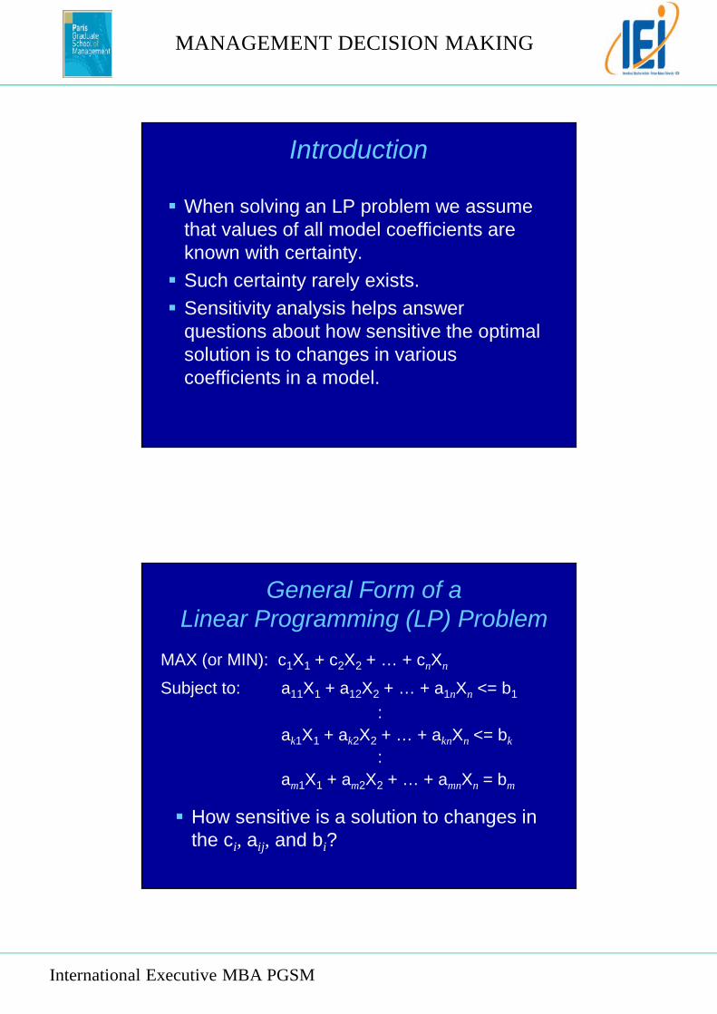
Introduction

When solving an LP problem we assumethat values of all model coefficients areknown with certainty. Such certainty rarely exists. Sensitivity analysis helps answer

questions about how sensitive the optimalsolution is to changes in variouscoefficients in a model.

General Form of aLinear Programming (LP) Problem

MAX (or MIN): c1X1 + c2X2 + … + cnXn

Subject to: a11X1 + a12X2 + … + a1nXn <= b1

:ak1X1 + ak2X2 + … + aknXn <= bk

:am1X1 + am2X2 + … + amnXn = bm

How sensitive is a solution to changes inthe ci, aij, and bi?



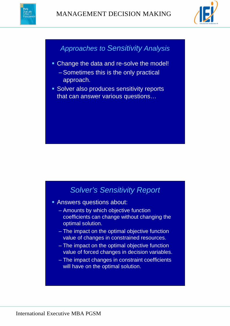
Approaches to Sensitivity Analysis

Change the data and re-solve the model!– Sometimes this is the only practical

approach. Solver also produces sensitivity reports

that can answer various questions…

Solver’s Sensitivity Report Answers questions about:

– Amounts by which objective functioncoefficients can change without changing theoptimal solution.

– The impact on the optimal objective functionvalue of changes in constrained resources.

– The impact on the optimal objective functionvalue of forced changes in decision variables.

– The impact changes in constraint coefficientswill have on the optimal solution.



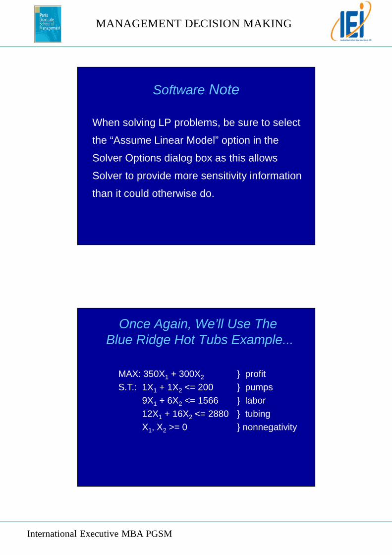
Software Note

When solving LP problems, be sure to select

the “Assume Linear Model” option in the

Solver Options dialog box as this allows

Solver to provide more sensitivity information

than it could otherwise do.

Once Again, We’ll Use TheBlue Ridge Hot Tubs Example...

MAX: 350X1 + 300X2 } profitS.T.: 1X1 + 1X2 <= 200 } pumps

9X1 + 6X2 <= 1566 } labor12X1 + 16X2 <= 2880 } tubingX1, X2 >= 0 } nonnegativity



The Answer Report

See file Fig4-1.xls

The Sensitivity Report

See file Fig4-1.xls



How Changes in Objective CoefficientsChange the Slope of the Level CurveX2

X1

250

200

150

100

50

00 50 100 150 200 250

new optimal solution

original level curve

original optimal solution

new level curve

How Changes in Objective CoefficientsChange the Slope of the Level Curve

See file Fig4-4.xls



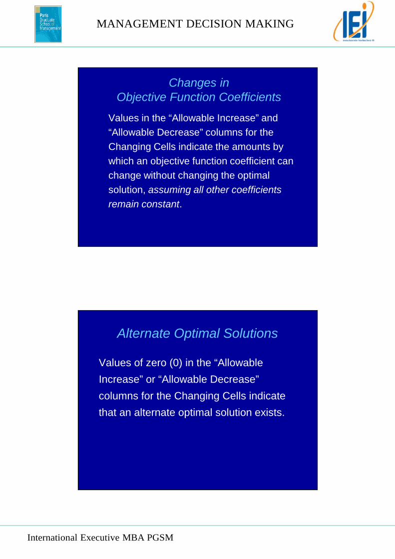
Changes inObjective Function Coefficients

Values in the “Allowable Increase” and“Allowable Decrease” columns for theChanging Cells indicate the amounts bywhich an objective function coefficient canchange without changing the optimalsolution, assuming all other coefficientsremain constant.

Alternate Optimal Solutions

Values of zero (0) in the “AllowableIncrease” or “Allowable Decrease”columns for the Changing Cells indicatethat an alternate optimal solution exists.



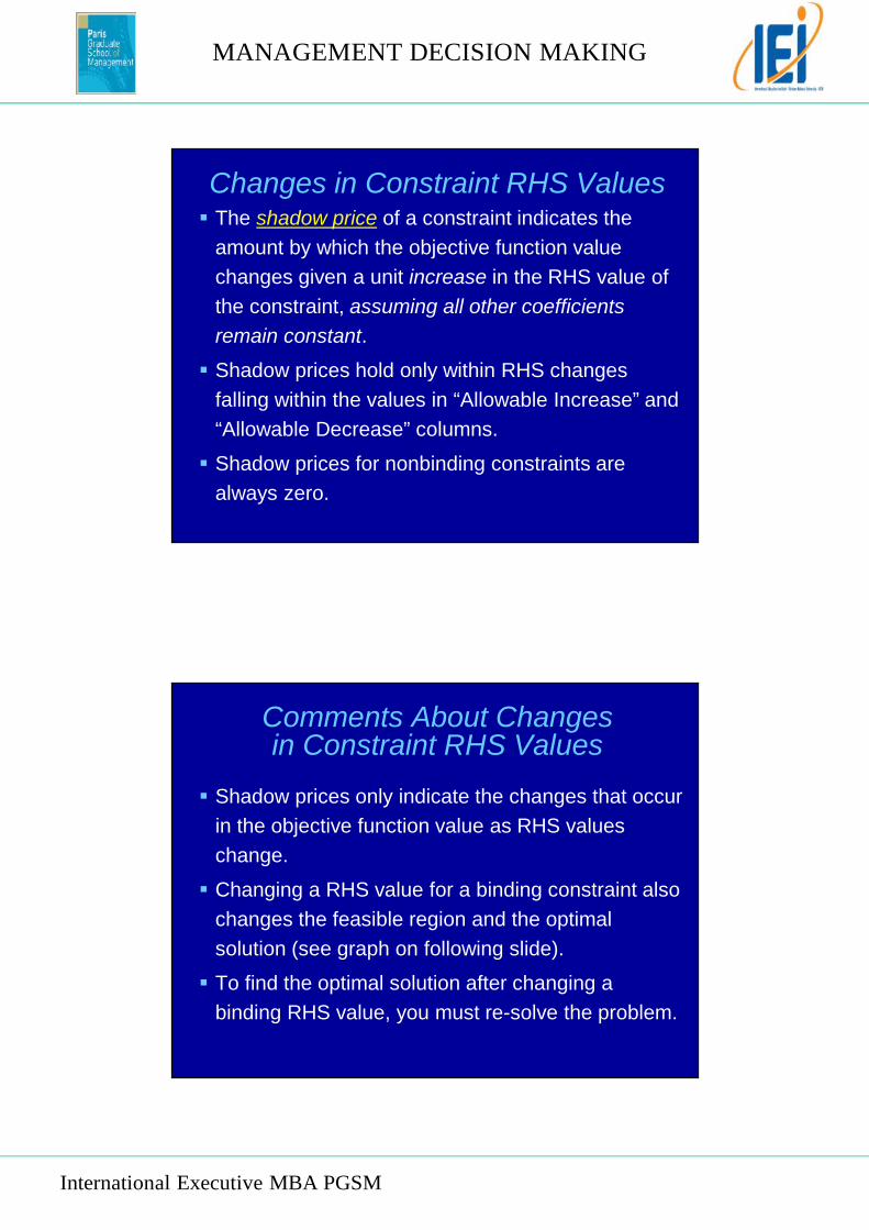
Changes in Constraint RHS Values The shadow price of a constraint indicates the

amount by which the objective function valuechanges given a unit increase in the RHS value ofthe constraint, assuming all other coefficientsremain constant.

Shadow prices hold only within RHS changesfalling within the values in “Allowable Increase” and“Allowable Decrease” columns.

Shadow prices for nonbinding constraints arealways zero.

Comments About Changesin Constraint RHS Values

Shadow prices only indicate the changes that occurin the objective function value as RHS valueschange.

Changing a RHS value for a binding constraint alsochanges the feasible region and the optimalsolution (see graph on following slide).

To find the optimal solution after changing abinding RHS value, you must re-solve the problem.



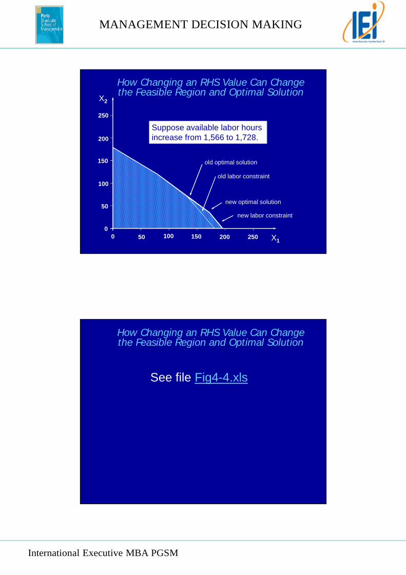
How Changing an RHS Value Can Changethe Feasible Region and Optimal Solution

X2

X1

250

200

150

100

50

00 50 100 150 200 250

old optimal solution

new optimal solution

old labor constraint

new labor constraint

Suppose available labor hoursincrease from 1,566 to 1,728.

See file Fig4-4.xls

How Changing an RHS Value Can Changethe Feasible Region and Optimal Solution



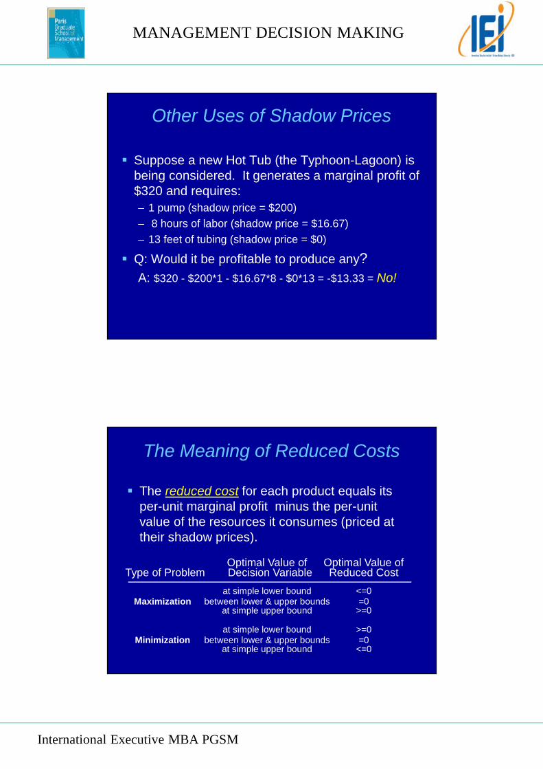
Other Uses of Shadow Prices

Suppose a new Hot Tub (the Typhoon-Lagoon) isbeing considered. It generates a marginal profit of$320 and requires:– 1 pump (shadow price = $200)– 8 hours of labor (shadow price = $16.67)– 13 feet of tubing (shadow price = $0)

Q: Would it be profitable to produce any?A: $320 - $200*1 - $16.67*8 - $0*13 = -$13.33 = No!

The Meaning of Reduced Costs

The reduced cost for each product equals itsper-unit marginal profit minus the per-unitvalue of the resources it consumes (priced attheir shadow prices).

Optimal Value of Optimal Value ofType of Problem Decision Variable Reduced Cost

at simple lower bound <=0Maximization between lower & upper bounds =0

at simple upper bound >=0

at simple lower bound >=0Minimization between lower & upper bounds =0

at simple upper bound <=0



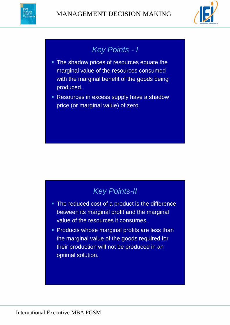
Key Points - I The shadow prices of resources equate the

marginal value of the resources consumedwith the marginal benefit of the goods beingproduced.

Resources in excess supply have a shadowprice (or marginal value) of zero.

Key Points-II The reduced cost of a product is the difference

between its marginal profit and the marginalvalue of the resources it consumes.

Products whose marginal profits are less thanthe marginal value of the goods required fortheir production will not be produced in anoptimal solution.



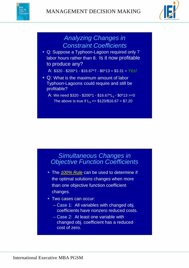
Analyzing Changes inConstraint Coefficients

Q: Suppose a Typhoon-Lagoon required only 7labor hours rather than 8. Is it now profitableto produce any?A: $320 - $200*1 - $16.67*7 - $0*13 = $3.31 = Yes!

Q: What is the maximum amount of laborTyphoon-Lagoons could require and still beprofitable?A: We need $320 - $200*1 - $16.67*L3 - $0*13 >=0

The above is true if L3 <= $120/$16.67 = $7.20

Simultaneous Changes inObjective Function Coefficients The 100% Rule can be used to determine if

the optimal solutions changes when morethan one objective function coefficientchanges. Two cases can occur:

– Case 1: All variables with changed obj.coefficients have nonzero reduced costs.

– Case 2: At least one variable withchanged obj. coefficient has a reducedcost of zero.



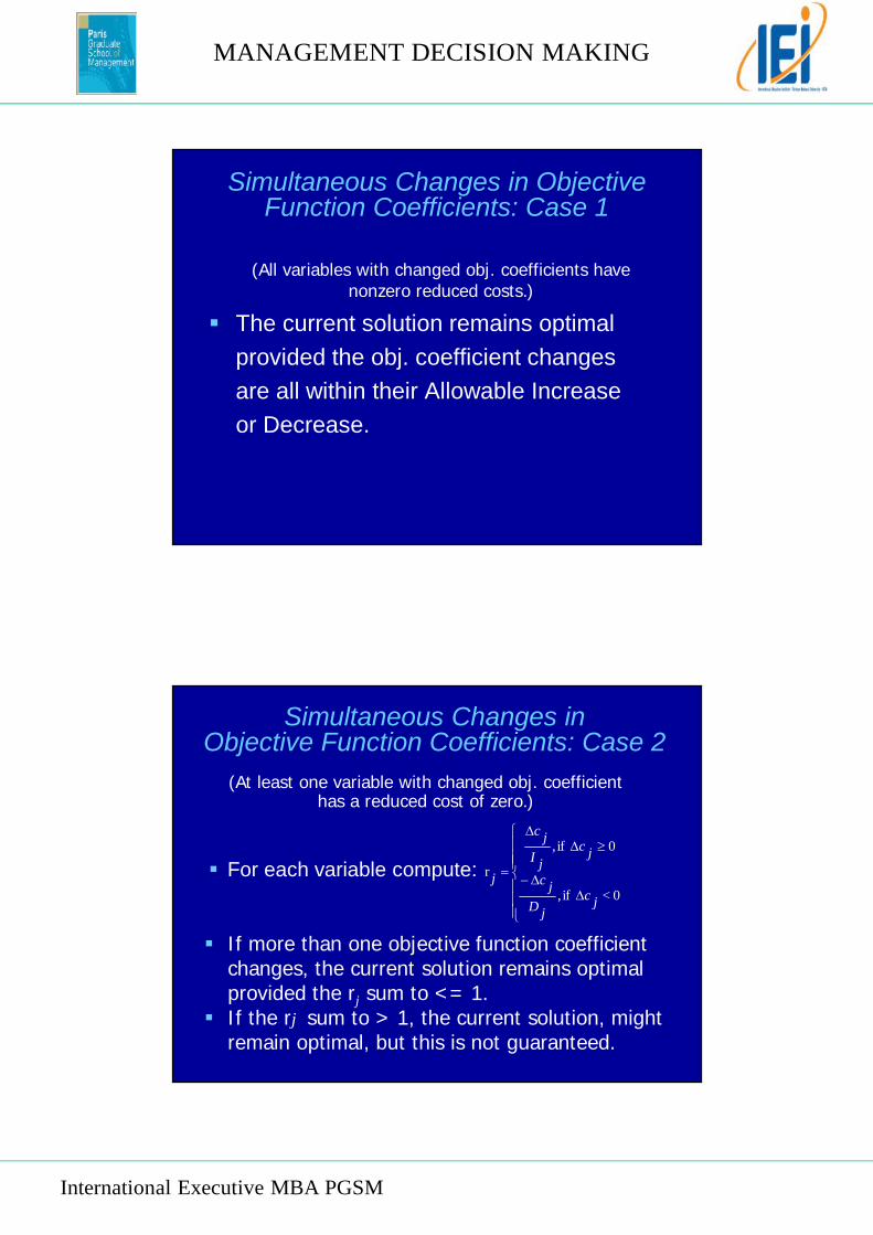
Simultaneous Changes in ObjectiveFunction Coefficients: Case 1

The current solution remains optimalprovided the obj. coefficient changesare all within their Allowable Increaseor Decrease.

(All variables with changed obj. coefficients havenonzero reduced costs.)

Simultaneous Changes inObjective Function Coefficients: Case 2

0<if,

0if,

r

jcjDjc

jcjIjc

j For each variable compute:

(At least one variable with changed obj. coefficienthas a reduced cost of zero.)

If more than one objective function coefficientchanges, the current solution remains optimalprovided the rj sum to <= 1.

If the rj sum to > 1, the current solution, mightremain optimal, but this is not guaranteed.



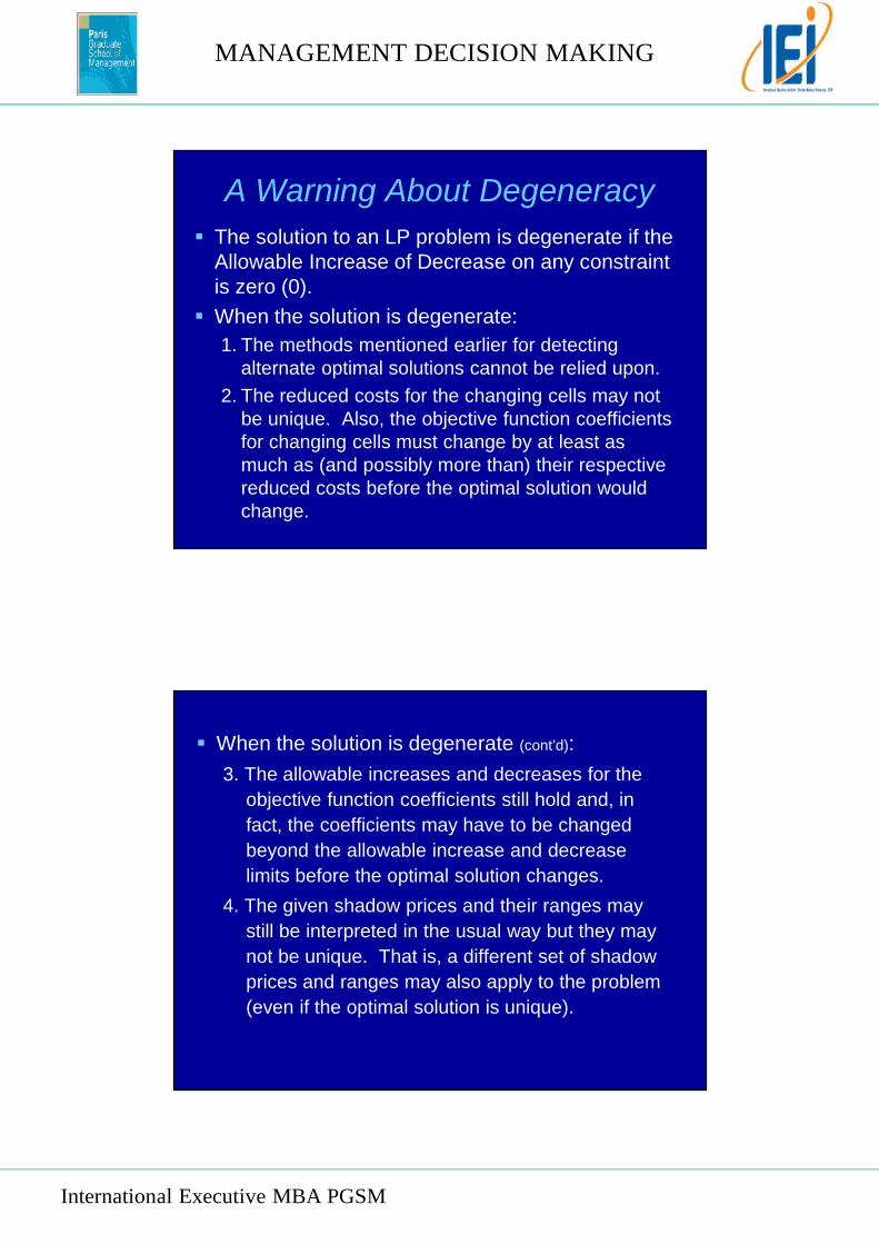
A Warning About Degeneracy The solution to an LP problem is degenerate if the

Allowable Increase of Decrease on any constraintis zero (0). When the solution is degenerate:

1. The methods mentioned earlier for detectingalternate optimal solutions cannot be relied upon.

2. The reduced costs for the changing cells may notbe unique. Also, the objective function coefficientsfor changing cells must change by at least asmuch as (and possibly more than) their respectivereduced costs before the optimal solution wouldchange.

When the solution is degenerate (cont’d):3. The allowable increases and decreases for the

objective function coefficients still hold and, infact, the coefficients may have to be changedbeyond the allowable increase and decreaselimits before the optimal solution changes.

4. The given shadow prices and their ranges maystill be interpreted in the usual way but they maynot be unique. That is, a different set of shadowprices and ranges may also apply to the problem(even if the optimal solution is unique).



The Limits Report

See file Fig4-1.xls

The Sensitivity Assistant

An add-in on the CD-ROM for this bookthat allows you to create:– Spider Tables & PlotsSummarize the optimal value for one output

cell as individual changes are made tovarious input cells.

– Solver TablesSummarize the optimal value of multiple

output cells as changes are made to asingle input cell.



The Sensitivity Assistant

See files:

Fig4-12.xls

&

Fig4-14.xls

The Simplex Method

For example: ak1X1 + ak2X2 + … + aknXn <= bk

converts to: ak1X1 + ak2X2 + … + aknXn + Sk = bk

And: ak1X1 + ak2X2 + … + aknXn >= bkconverts to: ak1X1 + ak2X2 + … + aknXn - Sk = bk

To use the simplex method, we first convert allinequalities to equalities by adding slackvariables to <= constraints and subtracting slackvariables from >= constraints.



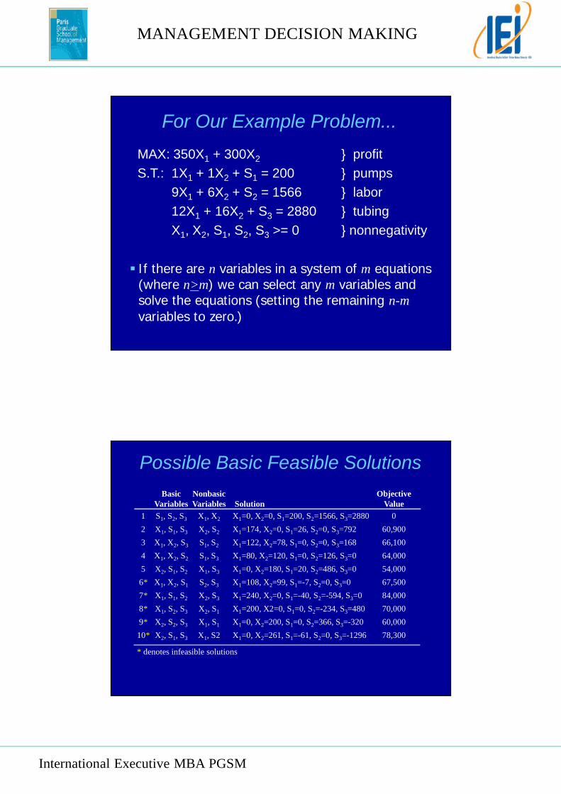
For Our Example Problem...MAX: 350X1 + 300X2 } profitS.T.: 1X1 + 1X2 + S1 = 200 } pumps

9X1 + 6X2 + S2 = 1566 } labor12X1 + 16X2 + S3 = 2880 } tubingX1, X2, S1, S2, S3 >= 0 } nonnegativity

If there are n variables in a system of m equations(where n>m) we can select any m variables andsolve the equations (setting the remaining n-mvariables to zero.)

Possible Basic Feasible SolutionsBasic Nonbasic Objective

Variables Variables Solution Value1 S1, S2, S3 X1, X2 X1=0, X2=0, S1=200, S2=1566, S3=2880 02 X1, S1, S3 X2, S2 X1=174, X2=0, S1=26, S2=0, S3=792 60,9003 X1, X2, S3 S1, S2 X1=122, X2=78, S1=0, S2=0, S3=168 66,1004 X1, X2, S2 S1, S3 X1=80, X2=120, S1=0, S2=126, S3=0 64,0005 X2, S1, S2 X1, S3 X1=0, X2=180, S1=20, S2=486, S3=0 54,0006* X1, X2, S1 S2, S3 X1=108, X2=99, S1=-7, S2=0, S3=0 67,5007* X1, S1, S2 X2, S3 X1=240, X2=0, S1=-40, S2=-594, S3=0 84,0008* X1, S2, S3 X2, S1 X1=200, X2=0, S1=0, S2=-234, S3=480 70,0009* X2, S2, S3 X1, S1 X1=0, X2=200, S1=0, S2=366, S3=-320 60,00010* X2, S1, S3 X1, S2 X1=0, X2=261, S1=-61, S2=0, S3=-1296 78,300

* denotes infeasible solutions



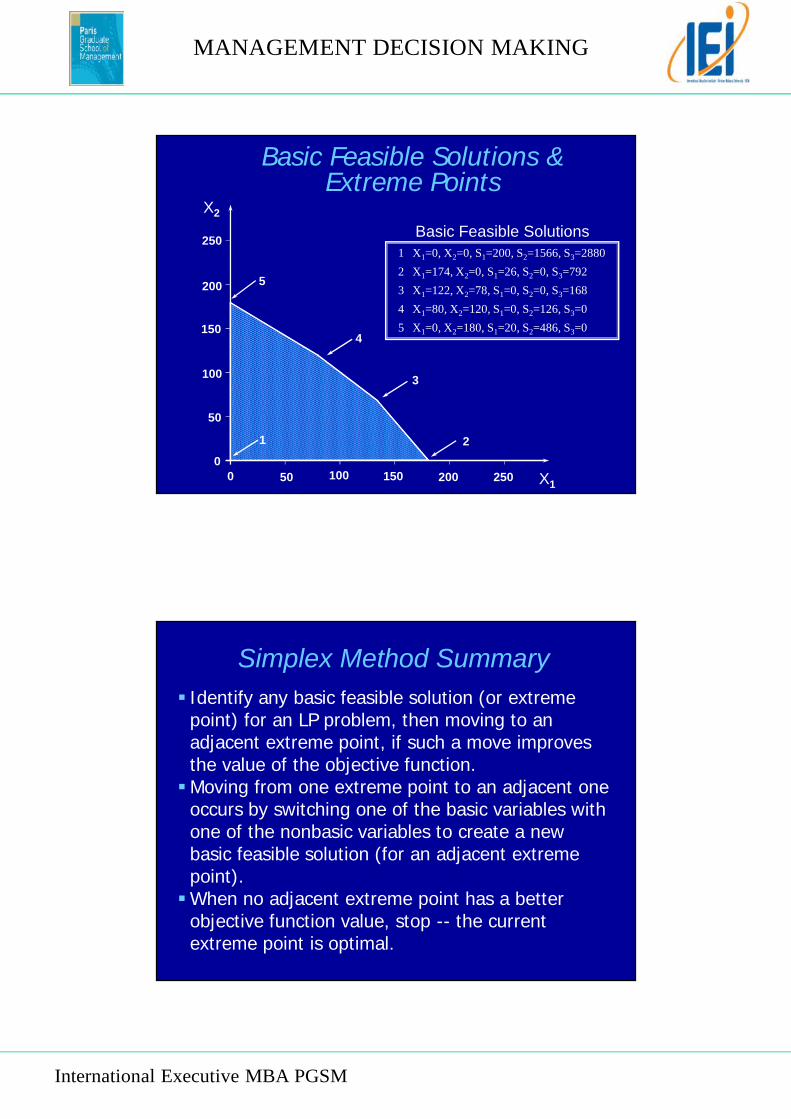
Basic Feasible Solutions &Extreme Points

X2

X1

250

200

150

100

50

00 50 100 150 200 250

5

2

3

4

1

1 X1=0, X2=0, S1=200, S2=1566, S3=28802 X1=174, X2=0, S1=26, S2=0, S3=7923 X1=122, X2=78, S1=0, S2=0, S3=1684 X1=80, X2=120, S1=0, S2=126, S3=05 X1=0, X2=180, S1=20, S2=486, S3=0

Basic Feasible Solutions

Simplex Method Summary Identify any basic feasible solution (or extreme

point) for an LP problem, then moving to anadjacent extreme point, if such a move improvesthe value of the objective function.Moving from one extreme point to an adjacent one

occurs by switching one of the basic variables withone of the nonbasic variables to create a newbasic feasible solution (for an adjacent extremepoint).When no adjacent extreme point has a better

objective function value, stop -- the currentextreme point is optimal.



End of Chapter 4

Economy & Finance

Reference 1