Embed Size (px)
Citation preview
Spatial GAS Models for Systemic Risk Measurement
SYstemic Risk TOmography:
Signals, Measurements, Transmission Channels, and Policy Interventions
Francisco Blasques (a,b)
Siem Jan Koopman (a,b,c) Andre Lucas (a,b,d) Julia Schaumburg (a,b) (a)VU University Amsterdam (b)Tinbergen Institute (c)CREATES (d)Duisenberg School of Finance
Workshop on Dynamic Models driven by the Score of Predictive Likelihoods La Laguna, January 9-11, 2014
This project has received funding from the European Union’s
Seventh Framework Programme for research, technological
development and demonstration under grant agreement no° 320270
www.syrtoproject.eu
This document reflects only the author’s views.
The European Union is not liable for any use that may be made of the information contained therein.
Introduction 3
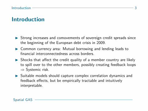
Introduction
I Strong increases and comovements of sovereign credit spreads sincethe beginning of the European debt crisis in 2009.
I Common currency area: Mutual borrowing and lending leads tofinancial interconnectedness across borders.
I Shocks that affect the credit quality of a member country are likelyto spill over to the other members, possibly creating feedback loops⇒ Systemic risk.
I Suitable models should capture complex correlation dynamics andfeedback effects, but be empirically tractable and intuitivelyinterpretable.
Spatial GAS
Introduction 4
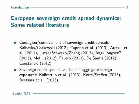
European sovereign credit spread dynamics:Some related literature
I Contagion/comovement of sovereign credit spreads:Kalbaska/Gatkowski (2012), Caporin et al. (2013), Aretzki etal. (2011), Lucas/Schwaab/Zhang (2013), Ang/Longstaff(2013), Metiu (2012), Favero (2013), De Santis (2012),Constancio (2012).
I Sovereign credit spreads vs. banks’ aggregate foreignexposures: Kallestrup et al. (2013), Korte/Steffen (2013),Beetsma et al. (2013).
Spatial GAS
Introduction 5
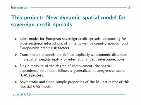
This project: New dynamic spatial model forsovereign credit spreads
I Joint model for European sovereign credit spreads, accounting forcross-sectional interactions of units as well as country-specific, andEurope-wide credit risk factors.
I Transmission channels are defined explicitly as economic distancesin a spatial weights matrix of international debt interconnections.
I Single measure of the degree of comovement, the spatialdependence parameter, follows a generalized autoregressive score(GAS) process.
I Asymptotic and finite sample properties of the ML estimator of this’Spatial GAS model’.
Spatial GAS
Outline 6
Outline
1. Introduction
2. Basic spatial lag model
3. Spatial lag model with GAS dynamics
4. Consistency of the Spatial GAS model
5. Simulation
6. Application: European CDS dynamics
7. Conclusions, Outlook
Spatial GAS
Spatial lag model 7
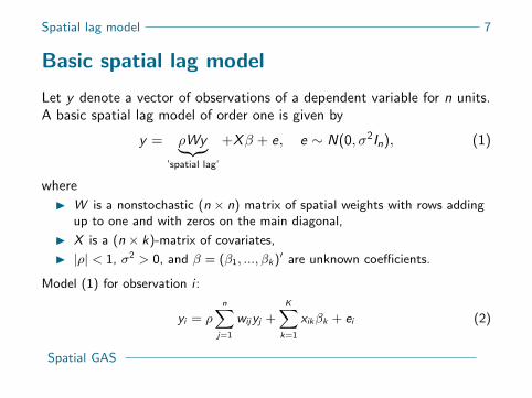
Basic spatial lag model
Let y denote a vector of observations of a dependent variable for n units.A basic spatial lag model of order one is given by
y = ρWy︸︷︷︸’spatial lag’
+Xβ + e, e ∼ N(0, σ2In), (1)
where
I W is a nonstochastic (n × n) matrix of spatial weights with rows addingup to one and with zeros on the main diagonal,
I X is a (n × k)-matrix of covariates,
I |ρ| < 1, σ2 > 0, and β = (β1, ..., βk)′ are unknown coefficients.
Model (1) for observation i :
yi = ρn∑
j=1
wijyj +K∑
k=1
xikβk + ei (2)
Spatial GAS
Spatial lag model 8
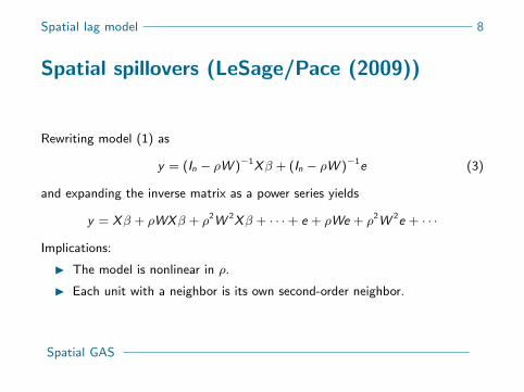
Spatial spillovers (LeSage/Pace (2009))
Rewriting model (1) as
y = (In − ρW )−1Xβ + (In − ρW )−1e (3)
and expanding the inverse matrix as a power series yields
y = Xβ + ρWXβ + ρ2W 2Xβ + · · ·+ e + ρWe + ρ2W 2e + · · ·
Implications:
I The model is nonlinear in ρ.
I Each unit with a neighbor is its own second-order neighbor.
Spatial GAS
Spatial lag model 9
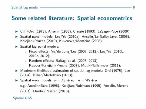
Some related literature: Spatial econometrics
I Cliff/Ord (1973), Anselin (1988), Cressie (1993), LeSage/Pace (2009);
I Spatial panel models: Lee/Yu (2010a), Anselin/Le Gallo/Jayet (2008),Kelejian/Prucha (2010), Kukenova/Monteiro (2008);
I Spatial lag panel models:
. Fixed effects: Yu/de Jong/Lee (2008, 2012), Lee/Yu (2010b,2010c, 2012);
. Random effects: Baltagi et al. (2007, 2013),
Kapoor/Kelejian/Prucha (2007), Mutl/Pfaffermayr (2011);
I Maximum likelihood estimation of spatial lag models: Ord (1975), Lee(2004), Hillier/Martellosio (2013);
I Spatial error models: y = Xβ + e, e = We + u
e.g. Anselin/Bera (1998), Kelejian/Robinson (1995), Anselin/Moreno
(2003), Chudik/Pesaran (2013).
Spatial GAS
Spatial lag model 10
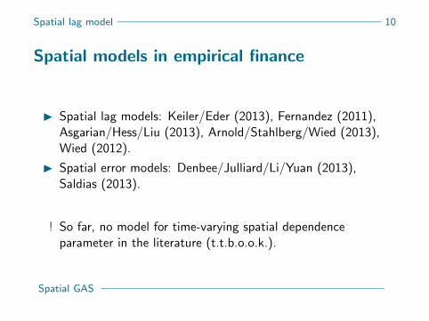
Spatial models in empirical finance
I Spatial lag models: Keiler/Eder (2013), Fernandez (2011),Asgarian/Hess/Liu (2013), Arnold/Stahlberg/Wied (2013),Wied (2012).
I Spatial error models: Denbee/Julliard/Li/Yuan (2013),Saldias (2013).
! So far, no model for time-varying spatial dependenceparameter in the literature (t.t.b.o.o.k.).
Spatial GAS
Spatial GAS 11
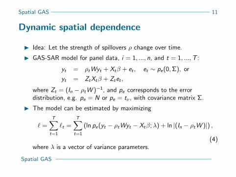
Dynamic spatial dependence
I Idea: Let the strength of spillovers ρ change over time.
I GAS-SAR model for panel data, i = 1, ..., n, and t = 1, ...,T :
yt = ρtWyt + Xtβ + et , et ∼ pe(0,Σ), or
yt = ZtXtβ + Ztet ,
where Zt = (In − ρtW )−1, and pe corresponds to the errordistribution, e.g. pe = N or pe = tν , with covariance matrix Σ.
I The model can be estimated by maximizing
` =T∑t=1
`t =T∑t=1
(ln pe(yt − ρtWyt − Xtβ;λ) + ln |(In − ρtW )|) ,
(4)where λ is a vector of variance parameters.
Spatial GAS
Spatial GAS 12
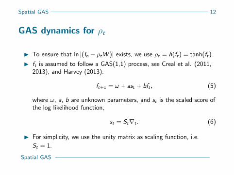
GAS dynamics for ρt
I To ensure that ln |(In − ρtW )| exists, we use ρt = h(ft) = tanh(ft).
I ft is assumed to follow a GAS(1,1) process, see Creal et al. (2011,2013), and Harvey (2013):
ft+1 = ω + ast + bft , (5)
where ω, a, b are unknown parameters, and st is the scaled score ofthe log likelihood function,
st = St∇t . (6)
I For simplicity, we use the unity matrix as scaling function, i.e.
St = 1.
Spatial GAS
Spatial GAS 13
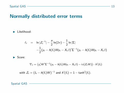
Normally distributed error terms
I Likelihood:
`t = ln |Z−1t | −
n
2ln(2π)− 1
2ln |Σ|
−1
2(yt − h(ft)Wyt − Xtβ)′Σ−1(yt − h(ft)Wyt − Xtβ)
I Score:
∇t =(y ′tW
′Σ−1(yt − h(ft)Wyt − Xtβ)− tr(ZtW ))· h′(ft)
with Zt = (In − h(ft)W )−1 and h′(ft) = 1− tanh2(ft).
Spatial GAS
Spatial GAS 14
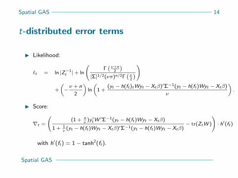
t-distributed error terms
I Likelihood:
`t = ln |Z−1t |+ ln
(Γ(ν+n
2
)|Σ|1/2(νπ)n/2Γ
(ν2
))
+
(−ν + n
2
)ln
(1 +
(yt − h(ft)tWyt − Xtβ)′Σ−1(yt − h(ft)Wyt − Xtβ)
ν
).
I Score:
∇t =
((1 + n
ν)y ′tW
′Σ−1(yt − h(ft)Wyt − Xtβ)
1 + 1ν
(yt − h(ft)Wyt − Xtβ)′Σ−1(yt − h(ft)Wyt − Xtβ)− tr(ZtW )
)· h′(ft)
with h′(ft) = 1− tanh2(ft).
Spatial GAS
Consistency 15
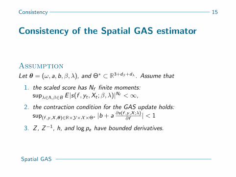
Consistency of the Spatial GAS estimator
AssumptionLet θ = (ω, a, b, β, λ), and Θ∗ ⊂ R3+dβ+dλ . Assume that
1. the scaled score has Nf finite moments:supλ∈Λ,β∈B E |s(f , yt ,Xt ;β, λ)|Nf <∞,
2. the contraction condition for the GAS update holds:
sup(f ,y ,X ,θ)∈R×Y×X×Θ∗ |b + a ∂s(f ,y ,X ;λ)∂f | < 1
3. Z , Z−1, h, and log pe have bounded derivatives.
Spatial GAS
Consistency 16
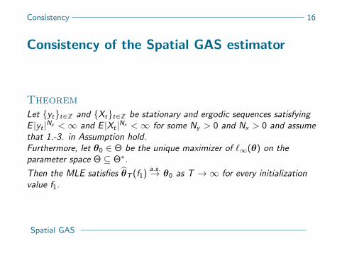
Consistency of the Spatial GAS estimator
TheoremLet {yt}t∈Z and {Xt}t∈Z be stationary and ergodic sequences satisfyingE |yt |Ny <∞ and E |Xt |Nx <∞ for some Ny > 0 and Nx > 0 and assumethat 1.-3. in Assumption hold.Furthermore, let θ0 ∈ Θ be the unique maximizer of `∞(θ) on theparameter space Θ ⊆ Θ∗.
Then the MLE satisfies θ̂T (f1)a.s.→ θ0 as T →∞ for every initialization
value f1.
Spatial GAS
Simulation 17
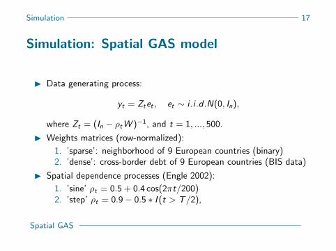
Simulation: Spatial GAS model
I Data generating process:
yt = Ztet , et ∼ i .i .d .N(0, In),
where Zt = (In − ρtW )−1, and t = 1, ..., 500.
I Weights matrices (row-normalized):
1. ’sparse’: neighborhood of 9 European countries (binary)2. ’dense’: cross-border debt of 9 European countries (BIS data)
I Spatial dependence processes (Engle 2002):
1. ’sine’ ρt = 0.5 + 0.4 cos(2πt/200)2. ’step’ ρt = 0.9− 0.5 ∗ I (t > T/2),
Spatial GAS
Simulation 18
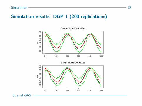
Simulation results: DGP 1 (200 replications)
0 100 200 300 400 500
0.0
0.2
0.4
0.6
0.8
1.0
Sparse W, MSE=0.00842
rho.
t
0 100 200 300 400 500
0.0
0.2
0.4
0.6
0.8
1.0
Dense W, MSE=0.01139
rho.
t
Spatial GAS
Simulation 19
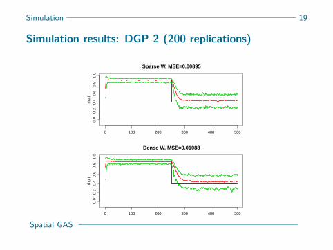
Simulation results: DGP 2 (200 replications)
0 100 200 300 400 500
0.0
0.2
0.4
0.6
0.8
1.0
Sparse W, MSE=0.00895
rho.
t
0 100 200 300 400 500
0.0
0.2
0.4
0.6
0.8
1.0
Dense W, MSE=0.01088
rho.
t
Spatial GAS
Application 20
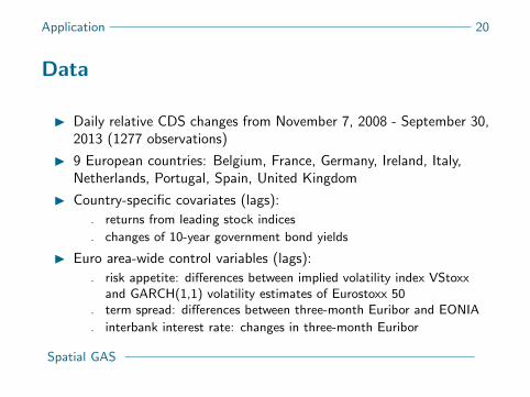
Data
I Daily relative CDS changes from November 7, 2008 - September 30,2013 (1277 observations)
I 9 European countries: Belgium, France, Germany, Ireland, Italy,Netherlands, Portugal, Spain, United Kingdom
I Country-specific covariates (lags):
. returns from leading stock indices
. changes of 10-year government bond yields
I Euro area-wide control variables (lags):
. risk appetite: differences between implied volatility index VStoxxand GARCH(1,1) volatility estimates of Eurostoxx 50
. term spread: differences between three-month Euribor and EONIA
. interbank interest rate: changes in three-month Euribor
Spatial GAS
Application 21
Spatial weights matrix
I Idea: Sovereign credit risk spreads are (partly) driven by cross-border debtinterconnections of the financial sector (see, e.g. Korte/Steffen (2013),Kallestrup et al. (2013)).
I Intuition: European banks are not required to hold capital buffers against
EU member states’ debt (’zero risk weight’). This can lead to
. regulatory arbitrage incentives and
. excessive issuing of of sovereign debt.
I If sovereign credit risk materializes, banks become undercapitalized andbailouts by domestic governments may be necessary, which in turn affectstheir credit quality.
I Entries of W : Row-standardized averages of quarterly across-the-border
debt exposures (Million US-$). Source: BIS homepage, Table 9B:
International bank claims, consolidated - immediate borrower basis.
Spatial GAS
Application 22
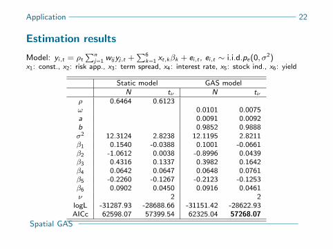
Estimation results
Model: yi,t = ρt∑n
j=1 wijyj,t +∑6
k=1 xt,kβk + ei,t , ei,t ∼ i.i.d.pe(0, σ2)x1: const., x2: risk app., x3: term spread, x4: interest rate, x5: stock ind., x6: yield
Static model GAS modelN tν N tν
ρ 0.6464 0.6123ω 0.0101 0.0075a 0.0091 0.0092b 0.9852 0.9888σ2 12.3124 2.8238 12.1195 2.8211β1 0.1540 -0.0388 0.1001 -0.0661β2 -1.0612 0.0038 -0.8996 0.0439β3 0.4316 0.1337 0.3982 0.1642β4 0.0642 0.0647 0.0648 0.0761β5 -0.2260 -0.1267 -0.2123 -0.1253β6 0.0902 0.0450 0.0916 0.0461ν 2 2
logL -31287.93 -28688.66 -31151.42 -28622.93AICc 62598.07 57399.54 62325.04 57268.07
Spatial GAS
Application 23
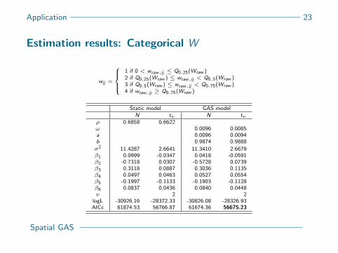
Estimation results: Categorical W
wij =
1 if 0 < wraw,ij ≤ Q0.25(Wraw )2 if Q0.25(Wraw ) ≤ wraw,ij < Q0.5(Wraw )3 if Q0.5(Wraw ) ≤ wraw,ij < Q0.75(Wraw )4 if wraw,ij ≥ Q0.75(Wraw )
Static model GAS modelN tν N tν
ρ 0.6858 0.6622ω 0.0096 0.0085a 0.0096 0.0094b 0.9874 0.9888
σ2 11.4287 2.6641 11.3410 2.6679β1 0.0999 -0.0347 0.0418 -0.0591β2 -0.7318 0.0307 -0.5728 0.0739β3 0.3118 0.0887 0.3036 0.1135β4 0.0497 0.0463 0.0527 0.0554β5 -0.1997 -0.1133 -0.1903 -0.1128β6 0.0837 0.0436 0.0840 0.0448ν 2 2
logL -30926.16 -28372.33 -30826.08 -28326.93AICc 61874.53 56766.87 61674.36 56675.23
Spatial GAS
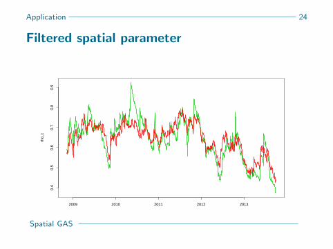
Application 24
Filtered spatial parameter
2009 2010 2011 2012 2013
0.4
0.5
0.6
0.7
0.8
0.9
rho_
t
Spatial GAS
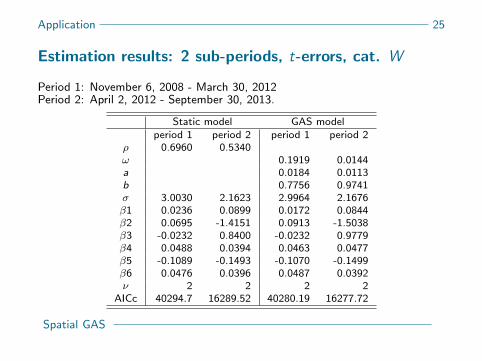
Application 25
Estimation results: 2 sub-periods, t-errors, cat. W
Period 1: November 6, 2008 - March 30, 2012Period 2: April 2, 2012 - September 30, 2013.
Static model GAS modelperiod 1 period 2 period 1 period 2
ρ 0.6960 0.5340ω 0.1919 0.0144a 0.0184 0.0113b 0.7756 0.9741σ 3.0030 2.1623 2.9964 2.1676β1 0.0236 0.0899 0.0172 0.0844β2 0.0695 -1.4151 0.0913 -1.5038β3 -0.0232 0.8400 -0.0232 0.9779β4 0.0488 0.0394 0.0463 0.0477β5 -0.1089 -0.1493 -0.1070 -0.1499β6 0.0476 0.0396 0.0487 0.0392ν 2 2 2 2
AICc 40294.7 16289.52 40280.19 16277.72
Spatial GAS
Application 26
Conclusions
I Spatial GAS model is new, and it works (theory, simulation).
I European sovereign CDS spreads are spatially dependent.Suitable spillover channel: debt interconnections.
I Best model: Spatial GAS with t-distributed errors andcategorical spatial weights.
I Some evidence for a level shift in spatial dependence afterGreek default (winter 2012).
Spatial GAS
Outlook 27
Outlook
I Theory:
. asymptotic normality of ML parameter estimator.
I Simulation:
. more DGPs for ρt ,
. t-distributed errors.
I Sovereign CDS application:
. check conditions implied by theory,
. significance of covariates,
. volatility clustering,
. other choices of W .
I Other application(s).
Spatial GAS