Embed Size (px)
DESCRIPTION
Citation preview


5887tp.cheanchian.04.05.ls 24/8/05 1:47 PM Page 2
The Fisher Modeland Financial Markets

This page intentionally left blankThis page intentionally left blank

5887tp.cheanchian.04.05.ls 24/8/05 1:47 PM Page 1
Richard D. MacminnIllinois State University, USA
The Fisher Model
and Financial Markets
World ScientficWorld ScientifcNEW JERSEY LONDON SINGAPORE BEIJING SHANGHAIO HONG KONG

Library of Congress Cataloging-in-Publication DataMacMinn, Richard D.
The Fisher model and financial markets / by Richard D. MacMinn.p. cm.
Includes bibliographical references and index.ISBN 981-256-407-1 (alk. paper) 1. Corporations--Finance--Mathematical models. 2. Finance--Mathematical models. I.
Title.
HG4012.M33 2005332'.01'5118--dc22
2005050603
British Library Cataloguing-in-Publication DataA catalogue record for this book is available from the British Library.
For photocopying of material in this volume, please pay a copying fee through the CopyrightClearance Center, Inc., 222 Rosewood Drive, Danvers, MA 01923, USA. In this case permission tophotocopy is not required from the publisher.
Typeset by Stallion PressEmail: [email protected]
All rights reserved. This book, or parts thereof, may not be reproduced in any form or by any means,electronic or mechanical, including photocopying, recording or any information storage and retrievalsystem now known or to be invented, without written permission from the Publisher.
Copyright © 2005 by World Scientific Publishing Co. Pte. Ltd.
Published by
World Scientific Publishing Co. Pte. Ltd.
5 Toh Tuck Link, Singapore 596224
USA office: 27 Warren Street, Suite 401-402, Hackensack, NJ 07601
UK office: 57 Shelton Street, Covent Garden, London WC2H 9HE
Printed in Singapore.

August 18, 2005 11:42 SPI-B312 The Fisher Model and Financial Markets (ED: Chean Chian) fm
Dedication
T his monograph grew out of a lecture on the Fisher Model and FinancialMarkets that I wrote in July of 1984. I subsequently presented it and
other lectures included here in my Ph.D. course on Uncertainty in Economicsand Finance from 1984 till 2000. My Ph.D. students were a source of inspi-ration and insight. I valued them then as students and value them now ascolleagues and friends. I dedicate this monograph to them.
v

August 18, 2005 11:42 SPI-B312 The Fisher Model and Financial Markets (ED: Chean Chian) fm
This page intentionally left blankThis page intentionally left blank

August 18, 2005 11:42 SPI-B312 The Fisher Model and Financial Markets (ED: Chean Chian) fm
Contents
Preface ix
Chapter 1 The Fisher Model with Certainty 1
Chapter 2 The Fisher Model 12
Chapter 3 Financial Values 22
Chapter 4 Fisher Separation 27
Chapter 5 More Values 37
Chapter 6 Corporate Finance Theorems 44
Chapter 7 Agency Problems 53
Chapter 8 Information Problems: Hidden Knowledge 67
Chapter 9 Corporate Risk Management 84
Chapter 10 Concluding Remarks 100
Bibliography 103
Index 107
vii

August 18, 2005 11:42 SPI-B312 The Fisher Model and Financial Markets (ED: Chean Chian) fm
This page intentionally left blankThis page intentionally left blank
August 18, 2005 11:42 SPI-B312 The Fisher Model and Financial Markets (ED: Chean Chian) fm
Preface
T his monograph represents work begun in July of 1984. Like a num-ber of economists making the transition to finance, I wanted to gain
some perspective on and appreciation for the finance discipline and, like oth-ers, I did not find a coherent perspective anywhere in the literature. Whilethe Fisher model (1930) had been used in a number of corporate financetexts to note the foundations of the net present value rule, e.g., Brealey andMyers (1991), it had not been developed further in textbooks as a perspec-tive for students of the finance discipline.1 This work represents an attemptto articulate corporate finance from a common perspective and model. Bygeneralizing the Fisher model to include risks, it is possible to exposit andprove the classic corporate finance theorems and to establish a commonfoundation for the discipline. For me it has been much like my first realanalysis course that provided the first opportunity to really learn the calcu-lus. Here the classic theorems of corporate finance are collected, stated, andsome are proved. The reader is challenged to prove corollaries and theoremsand to see how the model provides the fundamental building blocks for thediscipline.
The Fisher model is summarized in Chapter 1 and subsequently gen-eralized along the lines first used by Arrow and Debreu, i.e., see Arrow(1963) and Debreu (1959). A simple two-date Fisher model is constructed ina framework with all risk-averse agents and risks. The risks are the contractsexchanged now and paid then. The risk-averse agents exchange the risks and
1The Martin, Cox, and MacMinn text, i.e., Martin, J. D. et al. (1988). The Theory of Finance:Evidence and Applications. Dryden Press., subsequently provided more on the Fisher modelthan other texts but the Fisher perspective was not maintained, as I would have preferred.
ix

August 18, 2005 11:42 SPI-B312 The Fisher Model and Financial Markets (ED: Chean Chian) fm
x The Fisher Model and Financial Markets PREFACE
behave in a self-interested manner to maximize expected utility subject toany relevant constraints. Introducing stocks to allow the transfer of moneyfrom now to then increases the dimension of the problem but otherwiseleaves the standard constrained maximization problem, so common in stan-dard microeconomic theory, in place. The simple stock contracts introducedby Arrow are easily seen to form the basis for the financial markets;2 othersecurities such as corporate stocks and bonds are also introduced and valuedas portfolios of the Arrow securities.
The standard economic assumption that risk averse agents behave in aself-interested manner is examined in Chapter 4. The classic Fisher separationresult is that the agent selects the scale of an investment project independentof any preferences for consumption now versus then and the result followsfrom the notion that more is preferred to less, i.e., self-interested behavior.The investment scale selected by the agent is also the scale that maximizes netpresent value and so the classic Fisher separation result provides the founda-tion for that rule. The Fisher model has been extended here to include risksand risk-averse agents and so it is natural to consider how the self-interestedproprietor or chief executive officer will behave. After specifying the compen-sation scheme, the chief executive officer has a decision problem that involvesthe selection of a portfolio of securities on personal account and an invest-ment decision and financing decision on corporate account. A separationresult flows from this analysis in much the same way that the classic Fisherseparation result did. Similarly, the corporate objective function or equiva-lently the rule used by the manager in making decisions on corporate accountalso follows as a simple corollary. For some compensation schemes the cor-porate objective function is the maximization of current shareholder valuesubject to relevant constraints; hence, the analysis provides the foundationfor the corporate objective function. What is more, it shows the connectionbetween current shareholder value and net present value. The analysis alsoshows that the corporate objective function that is derived from this kind ofanalysis is not always current shareholder value. The compensation schemewill determine the objective function used by the manager and if the manageris compensated with stock options then the objective function becomes themaximization of the value of the stock option package. The maximizationof stock option value can result in the acquisition of too much risk by themanager.
2The Arrow securities payoff one currency unit in a particular state and zero otherwise. Hence,the securities are unit vectors in the space of financial payoffs. The securities form a basis, i.e.,minimal spanning set, for the financial markets. The Arrow securities are called basis stock herebecause of the analogy to linear algebra.

August 18, 2005 11:42 SPI-B312 The Fisher Model and Financial Markets (ED: Chean Chian) fm
PREFACE The Fisher Model and Financial Markets xi
More contracts and values are introduced in Chapter 5 to provide aslightly different interpretation of debt and equity and to provide the con-tracts necessary in some of the subsequent analysis.
The classic theorems in corporate finance are introduced and some areproved in Chapter 6. The early theorems of Modigliani and Miller are provedusing a few different methods and discussed in some detail because they areimportant to topics in subsequent chapters, e.g., the 1958 Modigliani–MillerTheorem has implications for corporate control and for risk management.Other theorems are stated but proved in subsequent chapters.
Agency problems similar to those discussed by Jensen and Meckling(1976) are introduced and discussed in Chapter 7. The classic principal-agent problem due to Ross (1973) is discussed here and reframed in a finan-cial market setting as an agency problem. The agency problem is often dueto a hidden action problem that will be discussed. The risk-shifting problemand the under-investment problem are both examples of the hidden actionproblem and a contracting solution is provided here for the risk shiftingproblem.
An agency problem may occur due to either a hidden action or a hid-den knowledge problem. The hidden knowledge problem is considered inChapter 8. One of the most well known implications of the hidden knowl-edge problem is found in Myers and Majluf’s pecking order theorem. Thepecking order theorem is demonstrated.
The notion of risk management is considered in Chapter 9. The corpo-ration has long been viewed as a nexus of contracts in corporate finance andthat perspective has generated a lot of insight. Even the organization of thediscipline reflects this view. Capital structure theorems are concerned witha set of contracts. The selection of a capital structure for the firm is a riskmanagement decision. Questions surrounding mergers and acquisitions arealso concerned with contract sets; the decision to acquire or divest assets isan example of a risk management decision. Similarly, the decision to hedgecurrency, commodity, or interest rate risk is also a risk management deci-sion. The chapter on risk management might be viewed as a logical extensionof this nexus of contracts conception of the corporation. Within this frame-work, a hedging theorem due to Froot et al. (1993) is stated and proved.

This page intentionally left blankThis page intentionally left blank

August 18, 2005 11:41 SPI-B312 The Fisher Model and Financial Markets (ED: Chean Chian) ch01
Chapter 1The Fisher Model with
Certainty
T he model introduced here was originally described by Fisher (1930)under conditions of perfect foresight. It is summarized here in prepara-
tion for the subsequent chapters on uncertainty.1 This model provides threeresults that form the foundations for the theory of corporate finance. Themodel shows how one may develop the notion of the time value of moneyor the interest rate in a financial market model, how one may separate thesavings decisions of individuals from the investment decisions of firms, andfinally why the net present value rule is appropriate for decision making. Allof these results flow from the Fisher model and so make it of central impor-tance in the development of corporate finance. The certainty version of themodel does not explain the existence of different rates of return on securitiesor other matters of concern but an uncertainty version of the model mightbe expected to provide insights and is developed in subsequent chapters;those chapters are all founded on what is developed here. Some remarks areincluded at the end of this chapter to outline what may be expected from amore general Fisher model.
Financial markets perform the role of allowing individuals and corpo-rations to transfer money between dates. The individual may save by trans-ferring dollars from the present to the future. The corporation may investand finance the investment by transferring dollars from the future to thepresent. The following model provides the theoretical foundation for the net
1Those familiar with the Fisher model should proceed to the next chapter.
1

August 18, 2005 11:41 SPI-B312 The Fisher Model and Financial Markets (ED: Chean Chian) ch01
2 The Fisher Model and Financial Markets CHAPTER1
present value rule and by extension the corporate objective function. It alsodemonstrates why we look to the financial markets to find the cost of capital.
In its simplest setting, this model of individual behavior incorporatesonly one time period and does not include uncertainty. The model is devel-oped in three steps. First, allowing the consumer to participate in the financialmarket, the individual’s savings decision is characterized.2 Second, the invest-ment frontier is introduced and consumer is given the role of firm proprietor;although the net present value rule has not been derived yet, we assume thatthe proprietor makes an investment decision on behalf of the firm using thatrule. This investment decision is in capital goods rather than financial assets.Third, the individual’s savings decision is restored and the individual is giventwo roles. One role is firm proprietor and the other is consumer. The individ-ual makes both decisions to maximize expected utility subject to the appro-priate constraints. It should be noted that no objective function for the firmsuch as net present value is assumed here. Allowing the individual to makean investment decision as firm proprietor and to make a savings decisionin the financial market as a consumer, the individual’s savings and invest-ment decisions are characterized. In the first and third steps, the individual isassumed to behave in accordance with her own self-interest. It is importantto note that we are not assuming that the individual makes any decisions tomaximize net present value. If any model is to demonstrate the importanceof the net present value rule, then that model must show that the individualfinds it optimal to use the rule. This result is demonstrated in case three.
Savings Decisions
Suppose the consumer stands at date zero and makes choices that will allocateincome and consumption across two dates t = 0 and 1, that we refer to asnow and then respectively. The consumer is endowed with some income nowand then. Let m = (m0, m1) denote the income pair, similarly let c = (c0, c1)denote the consumption pair; each pair represents dollars now and then.Suppose the consumer can borrow and lend at the known interest rate r. Thenthe consumer selecting a consumption pair also makes a savings decisions0 = m0 − c0; the savings choice yields (m0 − c0)(1 + r) dollars then. Theconsumer must make these consumption choices consistent with a budgetconstraint
c0 + c1
1 + r= m0 + m1
1 + r(1.1)
2Since there is no uncertainty, all financial assets must yield the same rate of return. Hence itis logical to suppose that there is only one financial asset and market. This will change whenuncertainty is introduced.

August 18, 2005 11:41 SPI-B312 The Fisher Model and Financial Markets (ED: Chean Chian) ch01
CHAPTER1
The Fisher Model with Certainty 3
Figure 1.1 The budget constraint.
The budget constraint represents all the consumption pairs that equate thepresent value of the consumption plan with that of the income stream. Thepoint m = (m0, m1) in Figure 1.1 represents the time pattern of the income.Note that (1 + r) is the absolute value of the slope of the budget constraintand corresponds to the increase in consumption then from each dollar savednow. A greater income either now or then yields a higher budget line throughthe new income pair. A greater interest rate yields a steeper budget line, sincegiving up a unit of consumption now would permit even more consump-tion then.
The consumer’s preferences are represented by an intertemporal utilityfunction u(c0, c1). The utility maps consumption pairs into real numbers,i.e., the larger the number the better the consumption pair. The consumer isassumed to prefer more to less and so utility increases with more consumptionnow and then. The utility function also contains information concerningthe consumer’s preference for more consumption now versus then and thispreference is consumer specific.
The preferences indicated by the utility function may be representedwith intertemporal indifference curves; consumption pairs on an indifferencecurve, of course, indicate the same utility while the higher indifference curvesrepresent greater utility. The absolute value of the slope of these curves atany consumption pair yields the individual’s intertemporal marginal rate ofsubstitution, i.e., mrs, and measures the value of consumption now in termsof consumption then. A steeper indifference curve corresponds to greater
August 18, 2005 11:41 SPI-B312 The Fisher Model and Financial Markets (ED: Chean Chian) ch01
4 The Fisher Model and Financial Markets CHAPTER1
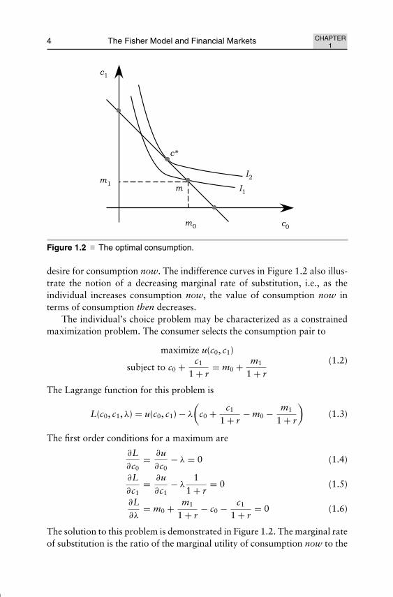
Figure 1.2 The optimal consumption.
desire for consumption now. The indifference curves in Figure 1.2 also illus-trate the notion of a decreasing marginal rate of substitution, i.e., as theindividual increases consumption now, the value of consumption now interms of consumption then decreases.
The individual’s choice problem may be characterized as a constrainedmaximization problem. The consumer selects the consumption pair to
maximize u(c0, c1)
subject to c0 + c1
1 + r= m0 + m1
1 + r(1.2)
The Lagrange function for this problem is
L(c0, c1, λ) = u(c0, c1) − λ
(c0 + c1
1 + r− m0 − m1
1 + r
)(1.3)
The first order conditions for a maximum are
∂L∂c0
= ∂u∂c0
− λ = 0 (1.4)
∂L∂c1
= ∂u∂c1
− λ1
1 + r= 0 (1.5)
∂L∂λ
= m0 + m1
1 + r− c0 − c1
1 + r= 0 (1.6)
The solution to this problem is demonstrated in Figure 1.2. The marginal rateof substitution is the ratio of the marginal utility of consumption now to the

August 18, 2005 11:41 SPI-B312 The Fisher Model and Financial Markets (ED: Chean Chian) ch01
CHAPTER1
The Fisher Model with Certainty 5
Figure 1.3 The investment frontier.
marginal utility of consumption then. From (1.4) and (1.5) it follows that
mrs =∂u∂c0
∂u∂c1
= λ
λ 11+r
= 1 + r (1.7)
Note that at the consumption bundle c∗, the consumer’s marginal rate ofsubstitution equals one plus the rate of interest, i.e., mrs∗ = 1 + r. The opti-mality condition has a simple interpretation; it says that at the margin c∗
the individual values consumption now in terms of consumption then at itsopportunity cost.
The Investment Frontier
Next suppose the time pattern of income may be altered by investing in capitalgoods. Let I0 denote the dollar investment in capital goods and �1 denotethe total dollar return on the investment; let �1 = �(I0) and suppose �(I0),i.e., the investment frontier, is a function which increases at a decreasingrate in the dollar investment. The function � is shown in Figure 1.3. Theslope of the investment frontier at a point is �′(I0) ≡ 1 + i(I0), where i isan interest rate called the marginal efficiency of investment. Since the payoff�1 increases at a decreasing rate, the marginal efficiency of investment alsodecreases as I0 increases.

August 18, 2005 11:41 SPI-B312 The Fisher Model and Financial Markets (ED: Chean Chian) ch01
6 The Fisher Model and Financial Markets CHAPTER1
The net present value and internal rate of return
Although the firm proprietor is not necessarily concerned with the net presentvalue, or equivalently, the net future value, of the investment project, it isappropriate at this point to identify the investment level which maximizesthe net present value. Let npv and nfv denote net present and future value,respectively. Then
npv(I0) = −I0 + �(I0)1 + r
(1.8)
and
nfv(I0) ≡ (1 + r)npv(I0)
= −(1 + r)I0 + �(I0) (1.9)
Maximizing npv and nfv, of course, yields the same investment level. Thederivative of net future value with respect to the investment level is
dnfvdI0
= −(1 + r) + �′(I0)
= −(1 + r) + (1 + i(I0))
= 0 (1.10)
At the investment level which maximizes nfv, this derivative is zero and sothe interest rate in the financial market equals the marginal efficiency ofinvestment, i.e., r = i(I∗
0). This condition simply says that the last dollarinvested must yield the same rate of return as is available in the financialmarket. The investment I∗
0 is shown in Figure 1.4. Note that the verticaldistance between �(I0) and (1+r) I0 is the net future value and I∗
0 maximizesthis distance.
It is also possible to provide a graphical interpretation of the internal rateof return, i.e., IRR, on the project. The internal rate of return is implicitlydefined as that rate of return which yields a zero net present value, or equiv-alently, a zero net future value. Hence, the IRR(I0) is implicitly defined bythe condition
nfv(I0) = − (1 + IRR(I0)) I0 + �(I0) = 0 (1.11)
or equivalently, by the condition
1 + IRR(I0) = �(I0)I0
(1.12)
This shows that one plus the internal rate of return can be interpreted graph-ically as the slope of a cord from the origin to a point on the investment

August 18, 2005 11:41 SPI-B312 The Fisher Model and Financial Markets (ED: Chean Chian) ch01
CHAPTER1
The Fisher Model with Certainty 7
Figure 1.4 The investment that maximizes npv and nfv.
frontier. Note that if, as assumed, �(I0) increases at a decreasing rate thenthe internal rate of return decreases in I0.
The Optimal Investment and Savings Decisions
Finally, suppose the individual not only selects a consumption plan but alsoan investment plan in capital goods. The consumer then effectively becomesa single proprietor. The ability to invest in capital goods alters the individ-ual’s income pair from (m0, m1) to (m0 − I0, m1 + �(I0)). The constrainedmaximization problem becomes a choice not only of an optimal consumptionplan c∗ but also an optimal investment. Hence, the constrained maximizationproblem is
maximize u(c0, c1)
subject to c0 + c1
1 + r= m0 − I0 + m1 + �(I0)
1 + r
(1.13)
The budget constraint is simply the condition that the present value of con-sumption plan equals the present value of income stream. The position ofthe budget constraint is determined by the investment decision because thatdecision alters the income pair. The individual has two roles. One of theroles is as the proprietor of a firm. In that capacity the individual makes theinvestment decision. The other role is that of a consumer. In this capacity,the individual selects the pair (c0, c1), or equivalently, a savings level. The

August 18, 2005 11:41 SPI-B312 The Fisher Model and Financial Markets (ED: Chean Chian) ch01
8 The Fisher Model and Financial Markets CHAPTER1
Figure 1.5 Fisher separation.
feasible investment and consumption decisions are represented by the invest-ment frontier and the associated budget line, respectively, in Figure 1.5.
The Lagrange function for the constrained maximization problem in(1.13) is
L(c0, c1, I0, λ) = u(c0, c1) − λ
(c0 + c1
1 + r− (m0 − I0) − m1 + �(I0)
1 + r
)(1.14)
The first order conditions are (1.4), (1.5), and
∂L∂I0
= −λ
(1 − �′(I0)
1 + r
)= 0 (1.15)
∂L∂λ
= (m0 − I0) + m1 + �(I0)1 + r
− c0 − c1
1 + r= 0 (1.16)
Note that first order condition (1.15) yields i(I∗0) = r as the condition for
an optimal investment; this is the familiar marginal efficiency of investmentequal the interest rate common in other economic models. The individ-ual, in the role of proprietor, selects the investment level indicated by thepair (m0 − I∗
0, m1 + �(I∗0)). Then, the individual, in the role of consumer,
selects the consumption bundle indicated by the point c∗. Note that, at b

August 18, 2005 11:41 SPI-B312 The Fisher Model and Financial Markets (ED: Chean Chian) ch01
CHAPTER1
The Fisher Model with Certainty 9
the condition i(I∗0) = r holds, while at c the condition mrs = 1 + r holds.
Also, observe that the condition i(I∗0) = r does not depend on the individual’s
preferences and that it is the condition for a maximum net present value.An alternative intuitive explanation is as follows: The individual has pref-
erences consistent with the observation that more is preferred to less. Theindividual selects the investment plan (I∗
0, �(I∗0)) which maximizes the present
value of total income, because by doing so the individual obtains the highestpossible budget line in the financial market. To see this, note that the budgetline for any investment decision intersects the horizontal axis at
m0 − I0 + m1 + �(I0)1 + r
= m0 + m1
1 + r− I0 + �(I0)
1 + r
= m0 + m1
1 + r+ npv(I0) (1.17)
and the budget line maximizes this value and so it yields the greatest capabilityfor consumption now and then. This is the Fisher separation result, i.e., allindividuals, irrespective of their preference for consumption now versus then,select the same investment plan. Maximizing the present value of income isequivalent to maximizing the net present value of the investment. Recallthat the analysis was not begun with the objective of maximizing the netpresent value. The objective was to maximize the individual’s utility subjectto a budget constraint and this yielded the result that any individual makesthe investment decision to maximize net present value. Hence, the roles ofproprietor and consumer can be separated.
Remarks
The Fisher model is remarkably robust for such a simple construct. It pro-vides for a determination of an interest rate, for a Fisher separation theoremand for a derivation of the net present value rule. It is possible to derive thesupply of and demand for savings based on the model developed here and soit is possible to determine an equilibrium rate of interest; that has not beenpursued here because the analysis focuses on the development of corporatefinance theory. For this development, the separation theorem plays an impor-tant role because it shows that an individual making a savings decision onpersonal account and a capital investment decision on firm or proprietorshipaccount will separate the two decisions, in the sense that the capital invest-ment decision will be made without reference to intertemporal preferences forconsumption now versus then. Equivalently, the separation theorem showsthat the investment decision is driven by the more is preferred to less assump-tion but not intertemporal preferences because the financial market allows

August 18, 2005 11:41 SPI-B312 The Fisher Model and Financial Markets (ED: Chean Chian) ch01
10 The Fisher Model and Financial Markets CHAPTER1
the individual to reallocate consumption across time by borrowing or lend-ing. Finally, the model also provides a decision rule for the single proprietorand that rule is to make decisions that maximize net present value.
The certainty version of the Fisher model has its limitations. The certaintymodel cannot explain different rates of returns for securities. As one wouldexpect, the introduction of uncertainty provides the basis for explaining dif-ferent rates of return and much more. Portfolio Theory (Markowitz 1952),the Capital Asset Pricing Model (Sharpe 1964; Mossin 1966; Garman 1979),the Arbitrage Pricing Model (Garman 1979), etc., have all been developed toprovide various explanations in corporate finance but none have the capa-bility of integrating the results in one framework. The Fisher model does asthe subsequent chapters show. Arrow’s work on the allocation of risk (1963)provides the foundation for a generalized version of the Fisher model. Thesavings decision becomes a portfolio decision as is shown in the next chapter.The subsequent chapters provide a demonstration of some of the key resultsand insights in corporate finance reframed and motivated in the context ofthe Fisher model.
Suggested Problems
1. Suppose the individual has intertemporal preferences specified byu(c0, c1) = min{c0, c1}. Sketch the indifferences curves and show theoptimal consumption bundle.
2. Suppose the individual has the intertemporal preferences specified inthe last problem and an income pair such that m0 > m1. Does theindividual lend or borrow in the financial market? How does the lendingor borrowing decision change given an increase in the interest rate?
3. Let the investment frontier be specified as �(I0) = min{κI0, M} where κ
and M are positive constants. Sketch this frontier. Also provide a sketchof the marginal efficiency of investment and the internal rate of return.
4. Show that nfv(I0) > 0 implies IRR(I0) > r and that nfv(I0) < 0 impliesIRR(I0) < r.
5. Suppose �′ > 0 and �′′ < 0. Show that i < IRR for all positive invest-ment levels.
6. Provide a sketch of an investment frontier which would yield a negativenet present value for any positive level of investment.
7. Why is it reasonable to say that the financial market rate of return r isthe cost of capital?
8. Sketch the case in which any positive investment in a project yields anegative npv and show that the consumer\proprietor chooses not toinvest.

August 18, 2005 11:41 SPI-B312 The Fisher Model and Financial Markets (ED: Chean Chian) ch01
CHAPTER1
The Fisher Model with Certainty 11
Figure 1.6 Mutually exclusive projects.
9. Show how the proprietor’s investment choice is affected by a reductionin the interest rate r.
10. Suppose that the proprietor selects an investment level either greaterthan or less than the level b shown in Figure 1.5. Show that, in eithercase, the individual is worse off and that this result does not depend onwhether the individual is a borrower or lender.
11. Suppose the proprietor can invest in one of two mutually exclusiveprojects. Let �A and �B denote the investment frontiers for the twoprojects, so that �A(I0) is the revenue generated then if project A isselected and �B(I0) if project B is selected. The investment frontiers areshown in Figure 1.6. Show and explain the following:
a. The Fisher separation result holds in terms of which project is selectedas well as the scale at which the project is operated.
b. Specify the conditions under which project B will be selected overproject A.
c. Which project has the larger internal rate of return? If you selectproject A or B on the basis of which has the larger IRR, is yourchoice consistent with your analysis in (b)?

August 18, 2005 11:41 SPI-B312 The Fisher Model and Financial Markets (ED: Chean Chian) ch02
Chapter 2The Fisher Model
T he Fisher model has been noted as one of the foundations of corporatefinance for decades. In its classic form, the Fisher model (1930) posits
the existence of a financial market that allows individuals to transfer moneybetween dates at a known rate of interest.1 Let those dates be known as nowand then. Individuals have preferences over consumption now versus thenand may implement those choices by saving or dissaving or equivalently bylending or borrowing in the financial market. Each individual makes a con-sumption choice that reallocates that individual’s income stream. The choiceis made to maximize utility subject to a budget constraint that limits choicesto those that make the present value of the consumption stream equal to thatof the income stream. The model was developed for a certain rate of returnin the financial market. Some attention has subsequently been focused on thesavings decision under uncertainty, e.g., Sandmo (1970) and Kimball (1990).The focus here is somewhat different; the focus is on the most natural exten-sion of the classic Fisher model to a financial market in which the individuals,whom we will subsequently also call consumers or investors, allocate theirconsumption through time by selecting from a variety of assets. The modeldeveloped here is the basic construct for all the subsequent developments.2
1This classic model is also typically extended to allow the individual to make an investmentdecision, i.e., an investment in physical as opposed to financial capital. The extension will beconsidered in a subsequent chapter.2Also see Hirshleifer, J. (1965). “Investment Decision Under Uncertainty: Choice-TheoreticApproaches.” Quarterly Journal of Economics 79(4): 509–536. Hirshleifer provided a compar-ison of the Capital Asset Pricing Model and the Fisher model and was one of the motivations forthe current model that provides a more robust generalization of the Fisher model in a financialmarket setting.
12

August 18, 2005 11:41 SPI-B312 The Fisher Model and Financial Markets (ED: Chean Chian) ch02
CHAPTER2
The Fisher Model 13
Consider a competitive economy operating between the dates now andthen. Consumer i selects a consumption pair (ci0, ci1) where ci0 denotes con-sumption now and ci1 denotes consumption then. Let (mi0, mi1) denote theconsumer’s income now and then. Let ui(ci0, ci1) be the consumer’s increasingconcave utility function; ui expresses the individual’s preferences for con-sumption now versus then. To introduce uncertainty let (�, F , �i) denotethe probability space for consumer i, where � is the set of states of nature,F is the event space, and �i is the probability measure. We will ini-tially suppose that there are only a finite number of states of nature, i.e.,� = {ξ1, ξ2, ξ3, . . . , ξN}, and for graphical purposes we let N = 2; in thiscase, the event space F is the power set, i.e., the set of all subsets of �. Tomake the uncertainty operational, suppose that the consumer can transferdollars from now to then by purchasing one or more of N risky assets; eachbasis asset in a complete market model is a promise to pay one dollar if stateof nature ξ occurs and zero otherwise. Let p(ξ ) be the price of an asset thatyields one dollar in state ξ and zero otherwise.
Consumer and Investor Behavior
The consumer selects a consumption plan that specifies a consumption levelnow and a consumption level for each state of nature that may occur then. Inits classic form, the problem is stated as a constrained maximization problem.Due to the uncertainty concerning consumption then, we maximize expectedutility subject to a budget constraint. Therefore the problem may be statedas follows:
maximize∫
�
ui(ci0, ci1)d�i
subject to ci0 +∑�
p(ξ )ci1(ξ ) = mi0 +∑�
p(ξ )mi1(ξ )(2.1)
where the left hand side of the constraint is the risk adjusted present valueof consumption and the right hand side is the risk adjusted present value ofincome. The budget constraint is shown in Figure 2.1.
Given the finite number of states of nature, the expected utility may alsobe expressed as follows:
∫�
ui(ci0, ci1)d�i=∑�
ui(ci0, ci1(ξ ))ψi (2.2)

August 18, 2005 11:41 SPI-B312 The Fisher Model and Financial Markets (ED: Chean Chian) ch02
14 The Fisher Model and Financial Markets CHAPTER2
Figure 2.1 The budget constraint.
where ψi(ξ ) is the probability of state ξ . The problem may then be equiva-lently expressed as
maximize∑�
ui(ci0, ci1(ξ ))ψi
subject to ci0 +∑�
p(ξ )ci1(ξ ) = mi0 +∑�
p(ξ )mi1(ξ )(2.3)
The first order conditions, for an optimal consumption number appropriatelyplan, are: ∑
�
D1uiψi(ξ ) − λi = 03 (2.4)
D2uiψi(ζ ) − λip(ζ ) = 0, for all ζ ∈ � (2.5)
Note that (2.4) simply says that the Lagrange multiplier λi equals the expectedmarginal utility of consumption now. Also observe that, using (2.4), (2.5)may be equivalently expressed as
p(ζ ) = D2uiψi(ζ )∑� D1uiψi(ξ )
(2.6)
which says that the consumer will purchase state ζ claims up to the point atwhich its price equals the marginal rate of substitution, i.e., the rate at which
3The D1ui is notation for the partial derivative of the function ui with respect to its first argu-ment; similarly D2ui is the partial derivative with respect to the second argument.

August 18, 2005 11:41 SPI-B312 The Fisher Model and Financial Markets (ED: Chean Chian) ch02
CHAPTER2
The Fisher Model 15
the consumer is willing to sacrifice consumption now for more consumptionin state ζ equals the price now of consumption in state ζ .4
It is also possible to consider the problem from the perspective of aninvestor. The investor selects a portfolio of securities to transfer dollarsbetween dates and states. Let xi(ξ ) be the number of state ξ shares pur-chased by investor i. Then the investor’s problem may be rewritten in termsof the financial assets. Consumption now and then become
ci0 = mi0 −∑�
p(ξ )xi(ξ ) (2.7)
and
ci1(ξ ) = mi1(ξ ) + xi(ξ ) (2.8)
respectively. Now the investor’s problem can be stated, in unconstrainedform, as
maximize∑�
ui
(mi0 −
∑�
p(ξ )xi(ξ ), mi1(ξ ) + xi(ξ )
)ψi(ξ ) (2.9)
where the consumption pair is expressed in terms of the financial assets.The first order conditions for the maximization problem are of the followingform:
−p(ζ )∑�
D1uiψi(ξ ) + D2uiψi(ζ ) = 0, for all ζ ∈ � (2.10)
Note that these conditions may be restated as
p(ζ ) = D2uiψi(ζ )∑� D1uiψi(ξ )
(2.11)
as previously in (2.6). Alternatively, we may note that
p(ξ1)p(ξ2)
= D2ui(ci0, ci1(ξ1))D2ui(ci0, ci1(ξ2))
(2.12)
4Note that ζ is the Greek letter zeta. It and the Greek letter ω, i.e., omega, will be used throughoutthe analysis to denote particular states in �. To see that the right hand side is the marginal rateof substitution, take the differential of the expected utility function, set it equal to zero, andnote that this yields (∑
�
D1uiψi(ξ )
)dci0 + (D2uiψi(ξ ))dci1(ξ ) = 0
⇔ − dci0
dci1(ξ )= D2uiψi(ζ )∑
� D1uiψi(ξ )

August 18, 2005 11:41 SPI-B312 The Fisher Model and Financial Markets (ED: Chean Chian) ch02
16 The Fisher Model and Financial Markets CHAPTER2
The right hand side of (2.12) is the investor’s marginal rate of substitutionwhile the left hand side is the price ratio. So this condition says that theinvestor selects state one and two claims such that the rate at which she iswilling to sacrifice state two consumption for more state one consumptionand remain indifferent equals that rate at which she can exchange state twoclaims for state one claims.
Having expressed the consumer’s problem in a financial market setting,it is natural to consider the demand for the basis stock in this economy.These assets form the basis for the expression of all financial values. Sinceall other assets can be expressed in terms of a portfolio of the basis assets,those demands are perfectly elastic at the portfolio price or equivalently thearbitrage free price. The basis assets, however, may be expected to havedownward sloping demand functions. The following section considers thedevelopment of the basis stock demand for a special case. The derivation ofthe demand and comparative statics in general case is left as an exercise.
Basis Stock Demand
Consider the demand for the basis stock. Let xi(ξj) ≡ xij, ψi(ξj) ≡ ψij andp(ξj) ≡ pj. Similarly, let xi = (xi1, . . . , xiN) denote the portfolio of basisstock, let p = (p1, . . . , pN) denote the vector of basis stock prices andlet ψi = (ψi1, . . . , ψiN) denote the vector of state probabilities. Now con-sider a special case of the utility function that eliminates the income effect.Let ui(ci0, ci1) = − exp (−ai[ci0 + ci1]) denote the utility function and letHi(xi; p, ψi) denote the expected utility function, i.e.,5
Hi(xi; p, ψi) =∑
J
ui
mi0 −
∑J
pjxij, xij
ψij (2.13)
The use of this utility function is motivated by Arrow’s work. In a port-folio model with one safe asset and one risky asset, Arrow showed thatnon-increasing absolute risk aversion implies that the risky asset is a normalgood.6 Since the demand for any normal good is downward sloping and the
5This utility function yields a generalized form of the constant absolute risk aversion utilityfunction. Note that
D11ui = −aiD1ui, D22ui = −aiD2ui, D12ui = −aiD2ui, and D12ui = −aiD2ui
This analysis must be generalized to allow for any utility function characterized by a generalizedmeasure of decreasing absolute risk a version.6See Arrow, K. J. (1974). “The Theory of Risk Aversion.” Essays in the Theory of Risk-Bearing. North-Holland.

August 18, 2005 11:41 SPI-B312 The Fisher Model and Financial Markets (ED: Chean Chian) ch02
CHAPTER2
The Fisher Model 17
utility function assumed here satisfies a generalized notion of constant abso-lute risk aversion, it should follow that the demand functions are downwardsloping. Given two states of nature, the first order conditions are
D1Hi = −p1
∑J
D1uiψij + D2uiψi1 = 0
D2Hi = −p2
∑J
D1uiψij + D2uiψi2 = 0(2.14)
It follows that the demand for basis stock one is a function xi1(p; ψ) and theslope of the demand function is
D1xi1(p; ψ) = −
∣∣∣∣D13Hi D12Hi
D23Hi D22Hi
∣∣∣∣∣∣∣∣D11Hi D12Hi
D21Hi D22Hi
∣∣∣∣(2.15)
Since the second order conditions for a maximum are
D11Hi < 0 and∣∣∣∣D11Hi D12Hi
D21Hi D22Hi
∣∣∣∣ > 0 (2.16)
the demand for basis stock one is downward sloping if the numerator ispositive. Direct calculation yields D23Hi = aix1, D2Hi = 0 and
D13Hi = −∑
J
D1uiψij + p1xi1
∑J
D11uiψij − D21uixi1ψi1
= −∑
J
D1uiψij + aixi1D1Hi
= −∑
J
D1uiψij
< 0
(2.17)
since more is preferred to less, i.e., D1ui > 0. The sign of the determinant inthe numerator of (2.15) is∣∣∣∣D13Hi D12Hi
D23Hi D22Hi
∣∣∣∣ =∣∣∣∣− −
0 −∣∣∣∣ > 0 (2.18)
It follows that the demand for basis stock one is downward sloping as shownin Figure 2.2.
Next, consider how the demand for basis stock one is affected by a changein the probability of state one. Note that in this two state example ψi can betreated as the probability of state one; then 1 − ψi is the probability of state

August 18, 2005 11:41 SPI-B312 The Fisher Model and Financial Markets (ED: Chean Chian) ch02
18 The Fisher Model and Financial Markets CHAPTER2
Figure 2.2 Basis stock demand.
two. The change in basis stock one demand, given a change in the probabilityof state one, is
D3xi1(p, ψi) = ∂xi1
∂ψi= −
∣∣∣∣D15Hi D12Hi
D25Hi D22Hi
∣∣∣∣∣∣∣∣D11Hi D12Hi
D21Hi D22Hi
∣∣∣∣(2.19)
Direct calculation shows that D15Hi > 0, D25Hi < 0, and D12Hi < 0. Thisderivative is positive if and only if the numerator is negative. The sign of thedeterminant in the numerator of (2.19) is∣∣∣∣D15Hi D12Hi
D25Hi D22Hi
∣∣∣∣ =∣∣∣∣+ −− −
∣∣∣∣ < 0 (2.20)
and so it follows that an increase in the probability of state one increasesthe demand for basis stock one, as expected. Other things being equal, thisresult implies an increase in the price of basis stock one. It may also be notedthat there is a reduction in the demand for basis stock two since
D3xi2(p, ψi) = −
∣∣∣∣D11Hi D15Hi
D21Hi D25Hi
∣∣∣∣∣∣∣∣D11Hi D12Hi
D21Hi D22Hi
∣∣∣∣= −
∣∣∣∣− +− −
∣∣∣∣∣∣∣∣D11Hi D12Hi
D21Hi D22Hi
∣∣∣∣< 0 (2.21)
Other things being equal, this result implies a decrease in the price of basisstock two. Equivalently, ceteris paribus, the price ratio p1/p2 increases.Finally, it should be observed that the basis stock prices incorporate andaggregate the investors’ preferences and probability beliefs. Any aggregatechange in probability beliefs or risk preferences will result in a change in
August 18, 2005 11:41 SPI-B312 The Fisher Model and Financial Markets (ED: Chean Chian) ch02
CHAPTER2
The Fisher Model 19
the composition of basis stock prices. A change in the risk preferences orprobability beliefs of one investor will, of course, not change stock prices inthis competitive market system.
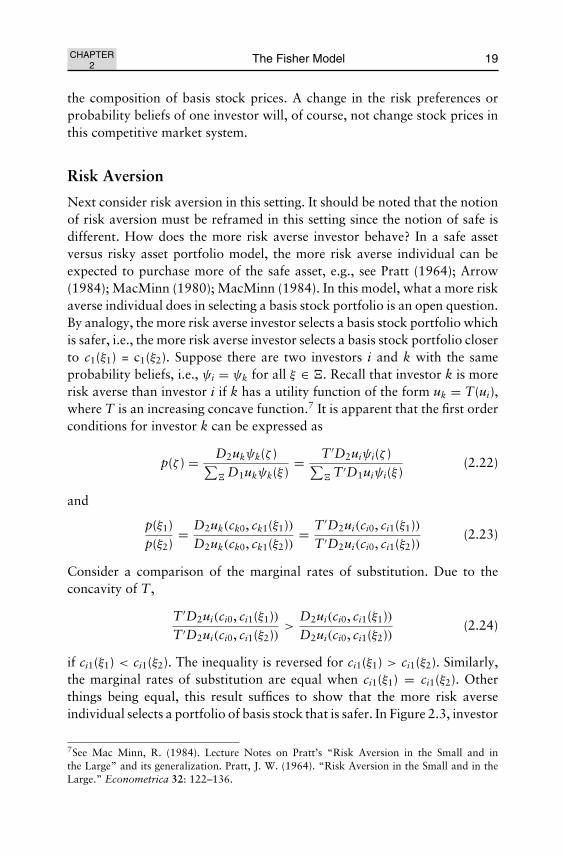
Risk Aversion
Next consider risk aversion in this setting. It should be noted that the notionof risk aversion must be reframed in this setting since the notion of safe isdifferent. How does the more risk averse investor behave? In a safe assetversus risky asset portfolio model, the more risk averse individual can beexpected to purchase more of the safe asset, e.g., see Pratt (1964); Arrow(1984); MacMinn (1980); MacMinn (1984). In this model, what a more riskaverse individual does in selecting a basis stock portfolio is an open question.By analogy, the more risk averse investor selects a basis stock portfolio whichis safer, i.e., the more risk averse investor selects a basis stock portfolio closerto c1(ξ1) = c1(ξ2). Suppose there are two investors i and k with the sameprobability beliefs, i.e., ψi = ψk for all ξ ∈ �. Recall that investor k is morerisk averse than investor i if k has a utility function of the form uk = T(ui),where T is an increasing concave function.7 It is apparent that the first orderconditions for investor k can be expressed as
p(ζ ) = D2ukψk(ζ )∑� D1ukψk(ξ )
= T ′D2uiψi(ζ )∑� T ′D1uiψi(ξ )
(2.22)
and
p(ξ1)p(ξ2)
= D2uk(ck0, ck1(ξ1))D2uk(ck0, ck1(ξ2))
= T ′D2ui(ci0, ci1(ξ1))T ′D2ui(ci0, ci1(ξ2))
(2.23)
Consider a comparison of the marginal rates of substitution. Due to theconcavity of T,
T ′D2ui(ci0, ci1(ξ1))T ′D2ui(ci0, ci1(ξ2))
>D2ui(ci0, ci1(ξ1))D2ui(ci0, ci1(ξ2))
(2.24)
if ci1(ξ1) < ci1(ξ2). The inequality is reversed for ci1(ξ1) > ci1(ξ2). Similarly,the marginal rates of substitution are equal when ci1(ξ1) = ci1(ξ2). Otherthings being equal, this result suffices to show that the more risk averseindividual selects a portfolio of basis stock that is safer. In Figure 2.3, investor
7See Mac Minn, R. (1984). Lecture Notes on Pratt’s “Risk Aversion in the Small and inthe Large” and its generalization. Pratt, J. W. (1964). “Risk Aversion in the Small and in theLarge.” Econometrica 32: 122–136.

August 18, 2005 11:41 SPI-B312 The Fisher Model and Financial Markets (ED: Chean Chian) ch02
20 The Fisher Model and Financial Markets CHAPTER2
Figure 2.3 Risk aversion.
one is more risk averse than investor two. The I1 and I2 denote indifferencecurves in consumption then space. Note that at individual two’s optimalconsumption pair, we have the following relation
mrs1 >p(ξ1)p(ξ2)
= mrs2 (2.25)
Since, from investor one’s perspective, the value of stock one in terms ofstock two exceeds the cost of stock one in terms of stock two, the more riskaverse investor can increase expected utility by substituting type one for typetwo stock.
Remarks
We have seen in each statement of the problem that the individual will havean incentive to hold more than one type of asset or stock in spite of thefact that the prices differ.8 This, of course, is due to risk aversion, i.e., therisk averse individual prefers a payoff in both states of nature to a payoff inonly one even if the prices of the assets differ. Hence this model provides anexplanation for the existence of different rates of return; recall that the rateof return on a basis stock that has a one dollar payoff in state ζ is
r(ζ ) = 1p(ζ )
− 1 (2.26)
and so if p(ζ ) > p(ξ ) it follows that r(ζ ) < r(ξ ).
8It need not be true that xi(ξ ) = 0 for all ξ ∈ �. However, even if xi(ξ ) = 0 it does not followthat the consumer is not selling shares in some corporation short because the corporations aresimply portfolios of the stocks modeled here.

August 18, 2005 11:41 SPI-B312 The Fisher Model and Financial Markets (ED: Chean Chian) ch02
CHAPTER2
The Fisher Model 21
Suggested Problems
1. Suppose the investor’s utility function takes the form u(c0, c1(ξ )) =−e−a(c0+c1(ξ )) where a is a positive constant. Show that the constant a canbe interpreted as a measure of absolute risk aversion. Will the investorhold the basis stock in fixed proportions independent of the measure ofabsolute risk aversion?
2. Suppose the investor’s utility function takes the form u(c0, c1(ξ )) =(c0 + c1(ξ ))1−r, where r is a positive constant less than one. Show thatr can be interpreted as a measure of relative risk aversion. Does this util-ity function provide a portfolio separation result?
August 18, 2005 11:41 SPI-B312 The Fisher Model and Financial Markets (ED: Chean Chian) ch03
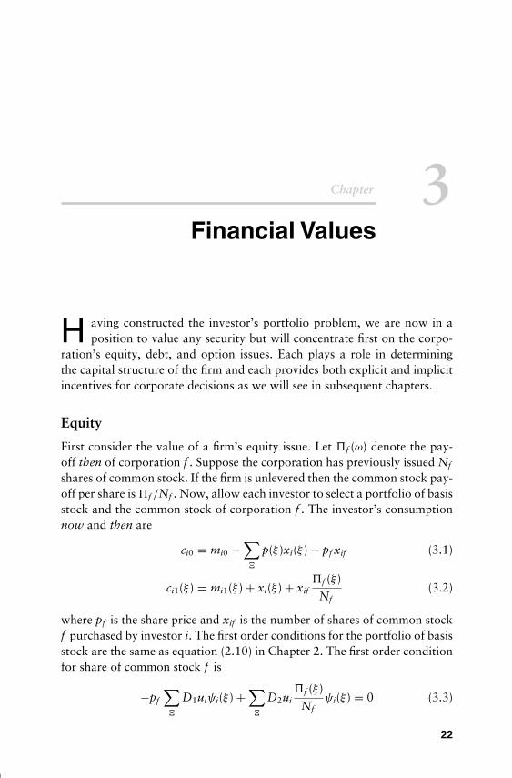
Chapter 3Financial Values
H aving constructed the investor’s portfolio problem, we are now in aposition to value any security but will concentrate first on the corpo-
ration’s equity, debt, and option issues. Each plays a role in determiningthe capital structure of the firm and each provides both explicit and implicitincentives for corporate decisions as we will see in subsequent chapters.
Equity
First consider the value of a firm’s equity issue. Let �f (ω) denote the pay-off then of corporation f . Suppose the corporation has previously issued Nf
shares of common stock. If the firm is unlevered then the common stock pay-off per share is �f /Nf . Now, allow each investor to select a portfolio of basisstock and the common stock of corporation f . The investor’s consumptionnow and then are
ci0 = mi0 −∑�
p(ξ )xi(ξ ) − pf xif (3.1)
ci1(ξ ) = mi1(ξ ) + xi(ξ ) + xif�f (ξ )
Nf(3.2)
where pf is the share price and xif is the number of shares of common stockf purchased by investor i. The first order conditions for the portfolio of basisstock are the same as equation (2.10) in Chapter 2. The first order conditionfor share of common stock f is
−pf
∑�
D1uiψi(ξ ) +∑�
D2ui�f (ξ )
Nfψi(ξ ) = 0 (3.3)
22

August 18, 2005 11:41 SPI-B312 The Fisher Model and Financial Markets (ED: Chean Chian) ch03
CHAPTER3
Financial Values 23
Using equation (2.11), it follows that the share price may be expressed as
pf =
∑�
D2ui�f (ξ )
Nfψi(ξ )∑
�D1uiψi(ξ )
=∑
�
D2uiψi(ζ )∑�
D1uiψi(ξ )
�f (ξ )Nf
=∑
�p(ξ )
�f (ξ )Nf
(3.4)
Alternatively, the stock market value of this unlevered corporation is Sf ,where
Sf ≡ pf Nf =∑�
p(ξ )�f (ξ ) (3.5)
Hence, the stock market value of the corporation is the risk adjusted presentvalue of its payoff, or equivalently, its quasi-rent.1
Debt
Next, consider the value of corporate bonds. Let a bond contract be a promiseto pay one dollar in each state of nature. Then it should be clear that the priceof the bond is pb, where pb is also a discount factor.
To reformulate the model to include debt, let pb be the price of a safe bondcontract and let yi be the number of bond contracts purchased by investor i.The individual’s consumption now and then become
ci0 = mi0 −∑�
p(ξ )xi(ξ ) − pf xif − pbyi (3.6)
ci1(ξ ) = mi1(ξ ) + xi(ξ ) + xif�f (ξ )
Nf+ yi (3.7)
The first order conditions for the safe bond contract is
∑�
[−pbD1ui + D2ui]ψi(ξ ) = 0 (3.8)
1The corporate payoff may be referred to as a quasi-rent in some cases because it does not includesome or all of the capital expenses that would be part of a previous investment expenditure.

August 18, 2005 11:41 SPI-B312 The Fisher Model and Financial Markets (ED: Chean Chian) ch03
24 The Fisher Model and Financial Markets CHAPTER3
Using the first order conditions (3.8) and equation (2.11), note that thiscondition may be rewritten as
pb =∑�
D2uiψi(ζ )∑� D1uiψi(ξ )
=∑�
p(ξ )(3.9)
This is the expected result since the safe debt contract is equivalent to pur-chasing one share of stock of each type ξ ∈ �. Any other result would yieldan arbitrage opportunity. Let bf be both the number of bond contracts andthe promised payment on the bond issue. It follows that the value of a safebond issue is Df (bf ) = pbbf .
Next, consider risky debt instruments. Suppose firm f has issued bondsfor which it promises to repay bf dollars at the end of the period if the firm’searnings are sufficient. Then the return to all bondholders is min{bf , �f }.The return per share is min{bf , �f }/bf = min{1, �f /bf } and so letting pbf
denote the share price of the corporation’s risky debt we have consumptionnow and then as
ci0 = mi0 −∑�
p(ξ )xi(ξ ) − pf xif − pbf yif (3.10)
ci1(ξ ) = mi1(ξ ) + xi(ξ ) + xif max
{0,
�f (ξ ) − bf
Nf
}+ yif min
{1,
�f (ξ )bf
}(3.11)
The first order condition for debt purchase becomes
∑�
[−pbf D1ui + D2ui min
{1,
�f
bf
}]ψi(ξ ) = 0 (3.12)
Let min{1, �f /bf } = 1 for all states of nature in the subset �\B and min{1,�f /bf } = �f /bf for all states of nature in the complement of �\B, i.e., B,then the first order condition (3.12) may be rewritten as
pbf =∑�\B
p(ξ ) +∑
B
p(ξ )�f (ξ )
bf(3.13)
Notice that the total market value of the firm’s risky debt is Df (bf ) = pbf bf ,or equivalently,
Df =∑�\B
p(ξ )bf +∑
B
p(ξ )�f (ξ )
=∑�
p(ξ ) min{�f (ξ ), bf }(3.14)

August 18, 2005 11:41 SPI-B312 The Fisher Model and Financial Markets (ED: Chean Chian) ch03
CHAPTER3
Financial Values 25
Figure 3.1 Values.
This result is also intuitively appealing because one bond is equivalent to aportfolio of stock with a one dollar payoff for all ξ ∈ �\B and with a fraction�f (ω)/bf of a dollar payoff for all ξ ∈ B.
By assuming a continuum of states of nature rather than a finite set, thebond and stock market values may be shown in Figure. 3.1.2 Let δ denote theboundary of the insolvency event, i.e., δ is implicitly defined by the condition�(δ) = b so that B = {ξ |�(ξ ) < b} = [0, δ). The bond or debt value isproportional to the green shaded area in Figure 3.1 and the equity value isproportional to the blue shaded area in the figure.
Call Options
Options are derivative instruments, i.e., instruments that derive their valuefrom other traded instruments. The call option will play a central role in muchof the analysis and so is considered here; other options will be considered insubsequent chapters. A call option on an asset gives its holder the right topurchase one share of the asset then at an exercise price established now. Ifthe call is written on the stock of corporation f then the payoff on the call is
2The shaded areas are not quite the values but they are proportional to them. For example, thecontinuous version of the debt value may be expressed as
D =∫
�
p(ξ ) min{b, �} dξ
= p(β)∫
�
min{b, �} dξ
for some β in �; this follows by the intermediate value theorem. A similar comment can bemade for the stock value.

August 18, 2005 11:41 SPI-B312 The Fisher Model and Financial Markets (ED: Chean Chian) ch03
26 The Fisher Model and Financial Markets CHAPTER3
max{0, (�f /Nf ) − ef } where ef is the exercise price. Let the call option pricebe cf . Then
cf =∑�
p(ξ ) max
{0,
�f (ξ )Nf
− ef
}(3.15)
The value of Nf such options is Cf , where
Cf ≡ cf Nf
=∑�
p(ξ ) max{0, �f (ω) − Ef } (3.16)
where Ef = ef Nf is the exercise value. Note that if bf = Ef then the stockmarket value of the levered firm is a call option value.
Suggested Problems
1. Define the rate of return for the stock of a levered corporation and showhow it changes with leverage.
2. Define the rate of return on the levered zero coupon bond.3. Define the weighted cost of capital and express it for the levered corpo-
ration. How does leverage affect the weighted cost of capital?
August 18, 2005 11:41 SPI-B312 The Fisher Model and Financial Markets (ED: Chean Chian) ch04
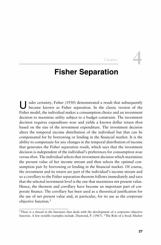
Chapter 4Fisher Separation
U nder certainty, Fisher (1930) demonstrated a result that subsequentlybecame known as Fisher separation. In the classic version of the
Fisher model, the individual makes a consumption choice and an investmentdecision to maximize utility subject to a budget constraint. The investmentdecision requires expenditure now and yields a known dollar return thenbased on the size of the investment expenditure. The investment decisionalters the temporal income distribution of the individual but that can becompensated for by borrowing or lending in the financial market. It is theability to compensate for any changes in the temporal distribution of incomethat generates the Fisher separation result, which says that the investmentdecision is independent of the individual’s preferences for consumption nowversus then. The individual selects that investment decision which maximizesthe present value of her income stream and then selects the optimal con-sumption pair by borrowing or lending in the financial market. Of course,the investment and its return are part of the individual’s income stream andso a corollary to the Fisher separation theorem follows immediately and saysthat the selected investment level is the one that maximizes net present value.Hence, the theorem and corollary have become an important part of cor-porate finance. The corollary has been used as a theoretical justification forthe use of net present value and, in particular, for its use as the corporateobjective function.1
1There is a thread in the literature that deals with the development of a corporate objectivefunction. A few notable examples include. Diamond, P. (1967). “The Role of a Stock Market
27

August 18, 2005 11:41 SPI-B312 The Fisher Model and Financial Markets (ED: Chean Chian) ch04
28 The Fisher Model and Financial Markets CHAPTER4
Now, consider whether Fisher’s results remain intact in this financialmarket model. In particular, it would be nice to see whether the Fisher sep-aration result holds here and what it implies about an objective function forthe publicly held and traded corporation. The corporate objective functionhas historically been assumed in much of the finance literature; there theassumptions include corporate value, stock value, current shareholder value,etc. One of the advantages of using Fisher’s approach to the construction of afinancial market model is that the corporate objective function can be derived.
A few cases are considered here in the process of generalizing the Fisherseparation theorem and its corollary. The first is in the spirit of the originalFisher model in which a single individual makes the consumption and invest-ment choices. We refer to that individual here as the sole proprietor and showthe first separation result. The next case considers what must motivate someof the thinking in corporate finance. In this second case the publicly heldand traded corporation is introduced. The corporate decisions are made by amanager who has a salary now and then and is also paid in corporate stock.In this case, a separation theorem is demonstrated that yields the expectedcorollary which says that the manager makes all decisions for the corpo-ration to maximize the current shareholder value and another immediatecorollary is that maximizing current shareholder value is equivalent to max-imizing risk adjusted net present value. Hence, all the expected results areconfirmed. Finally, the third case provides a different compensation schemefor the corporate manager. Since stock options were becoming common inthe last two decades of the 20th century, the manager is assumed to be givena compensation scheme that provides salary and stock options. A separationresult again holds and the corollary in this case yields an objective functionwhich says that the manager makes all decisions on corporate account tomaximize the value of the stock option package or equivalently the warrantvalue. Maximizing warrant value is easily shown to be inconsistent withmaximizing net present value.
in a General Equilibrium Model with Technological Uncertainty.” American Economic Review57: 759–773, Ekern, S. and R. Wilson (1974). “On the Theory of the Firm in an Economy withIncomplete Markets.” Bell Journal of Economics 5: 171–180, Radner, R. (1974). “A Note onUnanimity of Stockholder’s Preferences Among Alternative Production Plans: A Reformulationof the Ekern-Wilson Model.” Bell Journal of Economics 5: 181–184. This thread of the literatureis primarily concerned with the conditions that generate a corporate objective function that yieldsunanimity among the stakeholders of the corporate. Also see MacMinn, R. (1995). LectureNotes on Ekern and Wilson’s “On the Theory of the Firm in an Economy with IncompleteMarkets”.

August 18, 2005 11:41 SPI-B312 The Fisher Model and Financial Markets (ED: Chean Chian) ch04
CHAPTER4
Fisher Separation 29
Proprietor
First, consider the classic case of a single proprietorship. Let the proprietormake an investment decision on firm account as well as a portfolio decisionon personal account. Let �f (If , ω) be the earnings of firm f as a function notonly of the state of nature but also of the dollar investment If . The value offirm f is Vf where
Vf =∑�
p(ξ )�f (If , ξ ) (4.1)
We want to consider whether the proprietor’s decision on firm account isseparable from her decision on personal account. To allow the proprietor tomake the investment decision, let
ci0 = mi0 −∑�
p(ξ )xi(ξ ) − If (4.2)
and
ci1(ξ ) = mi1(ξ ) + xi(ξ ) + �f (If , ξ ) (4.3)
The unconstrained form for the proprietor’s decision problem is now
maximize∑�
ui
(mi0 −
∑�
p(ξ )xi(ξ ) − If , mi1(ξ )
+ xi(ξ ) + �f (If , ξ )
)ψi(ξ ) (4.4)
Then, in addition to the first order condition for basis stock, or equivalentlyequation (2.10), we have the condition for an optimal investment level givenbelow
−∑�
D1uiψi(ξ ) +∑�
D2ui D1�f ψi(ξ ) = 0 (4.5)
Using equation (2.11), this condition may be rewritten as∑�
p(ξ ) D1�f = 1 (4.6)
Since this condition for an optimal investment level does not depend on eitherthe risk aversion or probability measures of the proprietor, it follows that aFisher separation result holds here.

August 18, 2005 11:41 SPI-B312 The Fisher Model and Financial Markets (ED: Chean Chian) ch04
30 The Fisher Model and Financial Markets CHAPTER4
Note that the risk adjusted net present value of the investment If isVf − If . The maximum risk adjusted net present value is implicitly definedby the condition
∑�
p(ξ ) D1�f − 1 = 0 (4.7)
Hence, we see that the proprietor acting in her own interests will select theinvestment level that maximizes the risk adjusted net present value of thefirm. This is the standard corollary to the Fisher separation theorem.
It should be noted that although the investment decision will, other thingsbeing equal, change consumption now, it can be completely compensated forby altering the position in financial assets. The investment will also changethe risk of consumption then, but with complete markets that risk can bediversified. This result is particularly important because it generalizes thestandard Fisher separation result.
Corporation
Stock compensation scheme
Next, consider the manager of a publicly held and traded corporation. Sup-pose this manager or CEO makes all decisions on behalf of the corporationas well as personal decisions, i.e., personal portfolio decisions. Call the deci-sions for the corporation those on corporate account and call the personaldecisions those on personal account. Following one of the axioms of eco-nomic behavior, we will suppose that the manager makes all decisions in thepursuit of self-interest.
Suppose the manager makes the investment decision for the firm nowand uses a new stock issue to finance the investment. Let Sn
f denote the valueof the new stock issue and let If denote the dollar investment. Suppose thefirm has issued Nf + mf shares2 of stock previously and issues nf new sharesto finance the investment of If dollars. Note that the value of the new issue is
Snf =
∑�
p(ξ )nf
Nf + mf + nf�f (If , ξ)
= nf
Nf + mf + nfSf
(4.8)
2The mf shares will be noted later as those shares issued to the corporate manager as part ofher compensation scheme.

August 18, 2005 11:41 SPI-B312 The Fisher Model and Financial Markets (ED: Chean Chian) ch04
CHAPTER4
Fisher Separation 31
where Sf is the stock market value, i.e., the value of the new and old issues.The current stockholders have a fractional ownership of
1 − nf
Nf + mf + nf= Nf + mf
Nf + mf + nf(4.9)
and so the stock market value of the old shareholders’ position in the firm isSo
f , where
Sof = Nf + mf
Nf + mf + nfSf (4.10)
Now, suppose the manager issues enough new shares to just cover theinvestment expenditure of If dollars, i.e., Sn
f = If . Finally, note that the oldshareholders of the corporation want the manager to act in their interests,i.e., select the investment level to maximize So
f .Suppose the manager is partially paid in corporate stock now. Let mf
denote the number of shares held by the manager now and then.3 The cor-poration has Nf + mf shares outstanding now and issues an additional nf
shares to finance the new investment. The manager selects a savings level andportfolio on personal account and an investment level on corporate accountto solve the following constrained maximization problem
maximize∫
�
ui(ci0, ci1(ξ )) d�i(ξ )
subject to ci0 +∫
�
ci1(ξ ) dP(ξ ) = mi0 +∫
mi1(ξ ) dP(ξ )
+ mf
∫�
�f (If , ξ )Nf + mf + nf
dP(ξ )
andnf
Nf + mf + nf
∫�
�f (If , ξ ) dP(ξ ) = If
(4.11)
The last expression in (4.11) is the financing constraint. It determines thenumber of shares nf that must be issued now to raise the If dollars. Thepenultimate expression in (4.11) is the budget constraint that was representedin previous versions of the problem but with the addition of the last termon the right hand side. That addition to the budget constraint represents partof the compensation in the form of the manager’s stake in the equity value ofthe corporation. The investment decision that the manager makes will have
3We could allow the manager to trade shares of corporate stock now without changingthe following results as long as the manager has some equity stake in the corporation aftertrading.

August 18, 2005 11:41 SPI-B312 The Fisher Model and Financial Markets (ED: Chean Chian) ch04
32 The Fisher Model and Financial Markets CHAPTER4
an impact on the random payoff of the corporation and so its value. Theproblem may also be expressed in reduced form by noting that the financingconstraint implicitly defines a function nf (If ). Direct calculation yields
nf (If ) = If
Sf (If ) − If(Nf + mf ) (4.12)
Substituting this function into the budget constraint and simplifying yieldsthe constrained maximization problem in the following reduced form:
maximize∫
�
ui(ci0, ci1(ξ ))d�i(ξ )
subject to ci0 +∫
�
ci1(ξ )dP(ξ ) = mi0 +∫
�
mi1(ξ )dP(ξ )
+ mf
Nf + mf(Sf (If ) − If )
(4.13)
In this form it is clear that the manager makes decisions on corporate accountto maximize Sf − If . To see this, note that the first order conditions forthe decisions on personal account remain the same as those found in equa-tions (2.4) and (2.5); the condition for the investment decision on corporateaccount is
ddIf
(mf
Nf + mf(Sf (If ) − If )
)= mf
Nf + mf(S′
f (If ) − 1) = 0 (4.14)
The optimal investment decision is determined by that which makes themarginal stock value equal to the value of the last dollar invested. The deci-sion is separate from the manager’s time preferences and risk aversion. Hence,we have a Fisher separation result for the publicly held and traded corpora-tion. It may also be observed that the manager selects the investment levelto maximize the risk adjusted net present value, or equivalently, the currentshareholder value since Sf − If = Sf − Sn
f = Sof .
Stock option compensation scheme
The compensation of the manager may take a variety of forms. Each shouldyield a separation result with the corresponding corollary that specifies theobjective function. To see this, suppose the manager is partially paid in stockoptions now. Each option gives the manager the right to purchase one shareof corporate stock then at an exercise price of ef dollars. Suppose the manageris paid with mf options now. The corporation has Nf shares outstanding nowand issues an additional mf shares then if the manager exercises the options.Without loss of generality, suppose the firm issues bonds now to cover its

August 18, 2005 11:41 SPI-B312 The Fisher Model and Financial Markets (ED: Chean Chian) ch04
CHAPTER4
Fisher Separation 33
investment expenditure. The manager selects a consumption plan equiva-lently portfolio on personal account and an investment level on corporateaccount to solve the following constrained maximization problem
maximize∫
�
ui(ci0, ci1(ξ )) d�i(ξ )
subject to ci0 +∫
�
ci1(ξ ) dP(ξ ) = mi0 +∫
�
mi1(ξ ) dP(ξ )
+∫
�
max
{0,
mf
Nf + mf(�f (If , ξ )
+ ef mf − bf ) − ef mf
}dP(ξ )
and∫
�
min {�f (If , ξ ), bf } dP(ξ ) = If
(4.15)
The last expression in the problem is the financing constraint. It determinesthe promised payment bf on the debt issued now necessary to raise the If
dollars for the investment. The problem may also be expressed in reducedform by noting that the financing constraint implicitly defines a functionbf (If ). Substituting this function into the budget constraint and simplifyingyields the constrained maximization problem in the following reduced form:
maximize∫
�
ui(ci0, ci1(ξ )) d�i(ξ )
subject to ci0 +∫
�
ci1(ξ ) dP(ξ ) = mi0 +∫
�
mi1(ξ ) dP(ξ ) + Wf (If )(4.16)
where Wf represents the value of the stock option package, or equivalently,the warrant value. The warrant value may be equivalently expressed as
Wf (If ) =∫
�
max
{0,
mf
Nf + mf(�f (If , ξ ) − bf (If )) −
(1 − mf
Nf + mf
)Ef
}dP
(4.17)
where Ef = ef mf is the gross exercise value. It becomes clear in (4.16) that themanager will make decisions on corporate account to maximize the warrantvalue. Hence, we have another Fisher separation result for the publicly heldand traded corporation. It should also now be clear that the manager paid instock options does not have the incentive to make decisions that maximizecurrent shareholder value.
To note the difference in incentives, consider the investment choices madeby managers paid in stock versus stock options where the latter are not toodeeply in the money, i.e., there is some positive probability that the optionswill not be in the money when they vest then. The incentives for the cor-porate manager paid in stock options become clear when we compare the

August 18, 2005 11:41 SPI-B312 The Fisher Model and Financial Markets (ED: Chean Chian) ch04
34 The Fisher Model and Financial Markets CHAPTER4
investment decision of managers with different compensation schemes. Sup-pose, for example, that one corporate manager is paid in stock and anotheris paid in stock options. Suppose they have identical investment frontiers andboth can finance their choices with safe debt.4 The manager paid in stockoptions selects the investment level to maximize W(I) and so the first ordercondition is
W ′(Iw) = mf
Nf + mf
∫ ω
γ
(D1�(Iw, ξ ) − b′) dP(ξ ) = 0 (4.18)
where γ is the boundary of the exercise event and Iw denotes the investmentlevel implicitly defined by (4.18). The stock market value of the corporationthat finances with safe debt is
S(I) =∫ ω
0(�(I, ξ ) − b(I)) dP(ξ ) (4.19)
and the manager paid in stock selects the investment level to maximize S(I);the first order condition is
S′(Is) =∫ ω
0(D1�(Is, ξ ) − b′) dP(ξ ) = 0 (4.20)
Now to make a comparison of Iw and Is, suppose the investment frontiersatisfies the derivative properties D2� > 0 and D21� so that the Principleof Increasing Uncertainty (PIU) holds. Roughly put, this means that the riskof the investment increases in the size of the investment.5 Evaluating the firstorder condition (4.20) at Iw yields the following
S′(Iw) =∫ γ
0(D1�(Iw, ξ ) − b′) dP(ξ ) +
∫ ω
γ
(D1�(Iw, ξ ) − b′) dP(ξ )
=∫ γ
0(D1�(Iw, ξ ) − b′) dP(ξ )
< 0
(4.21)
4This assumption of safe debt is only made for convenience and simplicity. It does make thefunction b(I) implicitly defined by D(b) = I linear, i.e., b′ is a constant equal to one plus thesafe rate of return.5See Leland, H. (1972). “Theory of the Firm Facing Uncertain Demand.” American EconomicReview 62: 278–291, MacMinn, R. D. and A. Holtmann (1983). “Technological Uncertaintyand the Theory of the Firm.” Southern Economic Journal 50: 120–136. Leland defines theprinciple of increasing uncertainty using the derivative properties noted here and MacMinnshows that after correcting for the change in the mean of the payoff distribution, the increase inrisk can be interpreted as a Rothschild–Stiglitz increase in risk or equivalently a mean preservingspread of the payoff distribution, i.e., see Rothschild, M. and J. E. Stiglitz (1970). “IncreasingRisk: I. A Definition.” Journal of Economic Theory 2: 225–243.

August 18, 2005 11:41 SPI-B312 The Fisher Model and Financial Markets (ED: Chean Chian) ch04
CHAPTER4
Fisher Separation 35
The second equality in (4.21) follows by (4.18) and the inequality followsby the PIU. Equivalently, the inequality follows because D1� is monotoneincreasing and D1� − b′ negative for some state ξ > γ makes the integralon the right hand side of the second equality negative. Hence, the managerpaid in stock options selects a greater investment level, i.e., Iw > Is. Themanager paid in stock options takes on more risk than the manager paid instock.
Remarks
Each result here shows that the basic intuition of the certainty version of theFisher model continues to hold in this setting. The proprietor example is thesimplest extension of the Fisher result but the corporate manager examplesare more relevant. As long as the manager can diversify her portfolio onpersonal account, the motivation for decisions on corporate account willbe driven by the most basic axiom in economics, i.e., more is preferred toless. It should be noted that if the manager is paid with stock, then there isan alignment of interests with current shareholders and, what is more, themaximization of current shareholder value is equivalent to the net presentvalue rule for investment choices. If the manager is paid with stock options,then there is no general alignment of interests with shareholders. During thelast two decades of the 20th century, the seemingly unassailable argumentfor stock options was that the options would only be in the money if theshare price increased and so the connection between options and incentiveswas supposed to be obvious. That flawed logic, of course, ignored the risktaking incentives and the consequent impact on value. The more importantobservation here, however, is the general observation that the corollary toeach Fisher separation result yields a corporate objective function. Hence,the objective function is endogenous.
Suggested Problems
1. Suppose the manager’s compensation is a known salary now and then plusa bonus. Consider a few ways to construct a bonus scheme and derive themanager’s objective function for each.
2. Suppose the firm is producing a good or service and the manager mustmake a production decision q. Let �(q, ξ ) be the corporate payoff giventhe production decision q. Suppose the manager is paid in stock. If the firmis levered from a previous debt issue and b is the promised payment on

August 18, 2005 11:41 SPI-B312 The Fisher Model and Financial Markets (ED: Chean Chian) ch04
36 The Fisher Model and Financial Markets CHAPTER4
that debt, then derive the condition for an optimal production decision.Compare the optimal production decision for the case in which the riskof insolvency is zero versus that in which it is positive.
3. Claim: The manager paid with stock options has an incentive to takeovera target firm even if the net present value is non-positive. Prove it orprovide a counter example.

August 18, 2005 11:41 SPI-B312 The Fisher Model and Financial Markets (ED: Chean Chian) ch05
Chapter 5More Values
I n this chapter we want to value debt and equity using options and considerhow to value bond-warrant packages and convertible bond packages. The
subscript f for the corporation will be understood but not included here forsimplicity. The corporate value is the value of the firm’s debt plus equity andwill be denoted by V hereafter.
Call Options
A call option on an asset gives its holder the right to purchase one shareof the asset at the end of the period at an established exercise price. If thecall is written on the stock of corporation f then the payoff on the call ismax{0, (�/N) − e}. We have shown that the price of the call option is cwhere
c =∫
�
max
{0,
�(ξ )N
− e}
dP (5.1)
If the corporation issues N call options then C = cN is the market value ofits options. Therefore we have
C =∫
�
max{0, �(ξ ) − E} dP (5.2)
where E = eN. Next, recall that we have shown that the stock market valueof a levered corporation is S(b) where
S(b) =∫
�
max{0, �(ξ ) − b} dP = C (5.3)
37

August 18, 2005 11:41 SPI-B312 The Fisher Model and Financial Markets (ED: Chean Chian) ch05
38 The Fisher Model and Financial Markets CHAPTER5
Therefore the stock market value of the levered corporation may be inter-preted as the market value of a call option on the firm where b is the exercisevalue. Also recall that the value of the corporation’s debt issue is
D(b) =∫
�
min{�(ξ ), b} dP (5.4)
Since min{�, b} = �−max{0, �−b}, it follows that the corporate debt valuemay also be expressed as the value of the corporation minus the value of acall option on the corporation, i.e.,
D(b) =∫
�
[� − max{0, � − b}] dP
=∫
�
� dP −∫
�
max{0, � − b} dP
= V − C
(5.5)
Hence, it is possible to express the value of the levered corporation in termsof a call option. The bondholders purchase the asset, i.e., firm, and sell a calloption on the asset to stockholders.
Put Options
It is also possible to express the corporate debt and equity issues in terms ofputs. A put option on an asset gives its holder the right to sell the asset at theend of the period at an established exercise price. If the put is written on thestock of the corporation, then the payoff on the put is max{0, e − (�/N)}.Then the market value of the put option is p where
p =∫
�
max
{0, e − �(ξ )
N
}dP (5.6)
Note that if N puts are issued then the value of the put issue is
P ≡ pN =∫
�
max{0, E − �} dP (5.7)
where now E is the price at which the stock issue of the firm is sold, i.e., itsexercise value.
If we interpret the debt payment b as the exercise value, then we mayobserve that the stock market value of the levered corporation is the riskadjusted value of the firm’s earnings net of bond payments plus the value of

August 18, 2005 11:41 SPI-B312 The Fisher Model and Financial Markets (ED: Chean Chian) ch05
CHAPTER5
More Values 39
a put option on the firm. To see this, note that max{0, � − b} = � − b +max{0, b − �}. It follows that
S(b) =∫
�
(�(ξ ) − b) dP +∫
�
max{0, b − �(ξ )} dP
= V − B(b) + P(5.8)
where B(b) is the value of a safe debt issue. The stock market value of thelevered firm is the value of the firm minus the risk adjusted present value ofthe exercise price plus the value of the put. Equivalently, the stock marketvalue of the levered firm is its corporate value minus the value of a safedebt issue plus the value of the put. It is apparent that the put value may beinterpreted as the value of the shareholders’ limited liability. Similarly, sincemin{�, b} = b − max{0, b − �}, the corporate debt value is
D(b) =∫
�
b dP −∫
�
max{0, b − �(ξ )} dP
= B(b) − P(5.9)
Hence the debt value is the risk adjusted present value of the exercise priceminus the value of the put. Equivalently, it is the value of safe debt minusthe value of the put.
Bonds with Attached Warrants
Next, consider the value of a bond-warrant package. Suppose each bond isissued with a warrant which gives its owner the right to purchase γ (N +n)/bshares of stock at an exercise price of e per share of common stock. N is thenumber of shares now, while n is the number of new shares which must beissued then if the warrants are exercised. The fraction γ is simply n/(N + n).Note that a warrant is simply a call option. The payoff on a warrant is
max
{0, γ
N + nb
(� − b + E
N + n− e
)}(5.10)
and so the payoff on the entire warrant issue is
b max
{0, γ
N + nb
(� − b + E
N + n− e
)}= max
{0, γ
(� − b + E
) − E}
(5.11)where we define E as the exercise value of the warrant issue, i.e., E =eγ (N + n) = en. Then it follows easily that the market value of the warrant

August 18, 2005 11:41 SPI-B312 The Fisher Model and Financial Markets (ED: Chean Chian) ch05
40 The Fisher Model and Financial Markets CHAPTER5
Figure 5.1 Warrant value.
issue is
W(b, e, γ ) =∫
�
max{0, γ (� − b) − E} dP (5.12)
Note that the warrant is only exercised in the event that the firm is sol-vent. It follows that the bond-warrant holders have a payoff of min{�, b} +max{0, γ (�−b)−E}. Letting D(b, e, γ ) denote the market value of the bond-warrant package, note that
D(b, e, γ ) =∫
�
min{�(ξ ), b} dP +∫
�
max{0, γ (�(ξ ) − b) − E} dP
= D(b) + W(b, e, γ )(5.13)
as shown in Figure 5.2. Observe that (5.13) yields the result that the marketvalue of the package is equivalent to the value of a simple debt contract plusthe value of the warrant. The stockholders in this corporation have a payoffmax{0, � − b} − max{0, γ� − b) − E}. Hence, letting S(b, e, γ ) denote thestock market value of the firm with the bond-warrant package, we obtain
S(b, e, γ ) =∫
�
max{0, � − b} dP −∫
�
max{0, γ (� − b) − E} dP
= S(b) − W(b, e, γ )(5.14)
Hence, the stock market value of the firm with a bond-warrant package isequivalent to the stock market value of the firm with the simple debt contractminus the value of the warrant as shown in Figure 5.2. The 1958 Modigliani–Miller Theorem provided irrelevance result for corporate capital structurethat says that the value of the levered firm equals that of the unlevered.Letting b and n denote the size of the debt and equity issues, respectively,the theorem says that V(b, 0) = V(0, n) as will be demonstrated in the nextchapter. It may be noted that a generalization of the 1958 Modigliani–MillerTheorem follows here, since V(b, e, γ , 0) = V(b, 0) = V(0, n).

August 18, 2005 11:41 SPI-B312 The Fisher Model and Financial Markets (ED: Chean Chian) ch05
CHAPTER5
More Values 41
Figure 5.2 Stock value with a warrant issue.
Convertible Bonds
Next, consider convertible bonds. The convertible bond is a bond thatincludes a call option. It is similar to a bond with an attached warrant.The most obvious difference between the two is that the convertible bondowner surrenders the bond in order to exercise the option, while the bond-warrant owner surrenders cash in order to exercise the option. There areother differences including the fact that most warrants are detachable, whilethe option in the bond-call option package cannot be detached, and the factthat warrants, unlike many convertibles, cannot be called.
The feature of convertible bonds that makes them operational is the con-version ratio. Suppose that the bondholders acquire a fraction of the firm’sequity upon conversion and let the conversion ratio be θ = γ (N + n)/b,where γ ∈ (0, 1) and as before n is the number of shares that must be issuedthen if bondholders convert to stock. The payoff on a convertible bond is
max
{θ
�
N + n, min
{1,
�
b
}}= max
{γ
�
b, min
{1,
�
b
}}(5.15)
and the payoff on the convertible bond issue is
b max
{γ
�
b, min
{1,
�
b
}}= max{γ�, min{�, b}} (5.16)
Now, observe that the payoff may be equivalently expressed as
max{γ�, min{�, b}} = min{�, b} + max{0, γ� − min{�, b}}= min{�, b} + max{0, γ� − b} (5.17)

August 18, 2005 11:41 SPI-B312 The Fisher Model and Financial Markets (ED: Chean Chian) ch05
42 The Fisher Model and Financial Markets CHAPTER5
Figure 5.3 Call option value.
Therefore, letting D(b, γ ) denote the value of the convertible debt issue, itfollows that
D(b, γ ) =∫
�
min{�(ξ ), b} dP +∫
�
max{0, γ�(ξ ) − b} dP
= D(b) + C(b, γ )(5.18)
Hence, the value of convertible debt is simply the value of straight debt plusthe value of a call option. Since the bonds are converted if and only if thefirm is solvent, we may note that the payoff to stockholders is
min{max{0, � − b}, (1 − γ )�} = max{0, � − b}− max{0, � − b − (1 − γ )�}
= max{0, � − b} − max{0, γ� − b} (5.19)
Therefore, letting S(b, γ ) denote the stock market value of the firm withconvertible debt, we obtain
S(b, γ ) = S(b) − C(b, γ ) (5.20)
Again, it may be noted that the 1958 Modigliani–Miller irrelevance resultholds, i.e., V(b, γ , 0) = V(b, 0) = V(0, n). In fact the irrelevance result fol-lows by noting that the market values of the financial instruments are simplythe risk adjusted present values of the areas shown in Figure 5.3.
Suggested Problems
1. Consider a bond-warrant package. Specify the payoff on the bond-warrant and derive the value.

August 18, 2005 11:41 SPI-B312 The Fisher Model and Financial Markets (ED: Chean Chian) ch05
CHAPTER5
More Values 43
2. Suppose the corporation faces a random property loss of L dollars whereL : � → R and that the corporation may purchase insurance now for apremium of pi(d) given a deductible of d dollars, i.e., the insurance con-tract pays zero up to the deductible and then the loss minus the deductiblefor all larger losses. Provide an expression for the value of the insurancepremium.
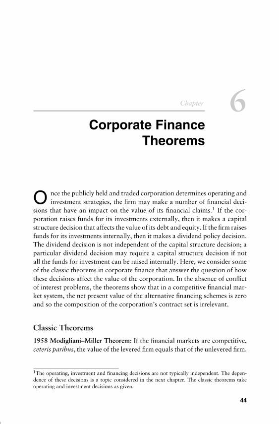
August 18, 2005 11:42 SPI-B312 The Fisher Model and Financial Markets (ED: Chean Chian) ch06
Chapter 6Corporate Finance
Theorems
O nce the publicly held and traded corporation determines operating andinvestment strategies, the firm may make a number of financial deci-
sions that have an impact on the value of its financial claims.1 If the cor-poration raises funds for its investments externally, then it makes a capitalstructure decision that affects the value of its debt and equity. If the firm raisesfunds for its investments internally, then it makes a dividend policy decision.The dividend decision is not independent of the capital structure decision; aparticular dividend decision may require a capital structure decision if notall the funds for investment can be raised internally. Here, we consider someof the classic theorems in corporate finance that answer the question of howthese decisions affect the value of the corporation. In the absence of conflictof interest problems, the theorems show that in a competitive financial mar-ket system, the net present value of the alternative financing schemes is zeroand so the composition of the corporation’s contract set is irrelevant.
Classic Theorems
1958 Modigliani–Miller Theorem: If the financial markets are competitive,ceteris paribus, the value of the levered firm equals that of the unlevered firm.
1The operating, investment and financing decisions are not typically independent. The depen-dence of these decisions is a topic considered in the next chapter. The classic theorems takeoperating and investment decisions as given.
44

August 18, 2005 11:42 SPI-B312 The Fisher Model and Financial Markets (ED: Chean Chian) ch06
CHAPTER6
Corporate Finance Theorems 45
The ceteris paribus is added here because it is implicit in the originalwork; no operating or investment decisions are made in conjunction with thecapital structure decision. Once the corporation has decided to raise fundsexternally, it may alter the amount it raises in the bond market versus thestock market. The 1958 Modigliani–Miller Theorem shows that, althoughan alteration in the size of the debt issue changes the value of the debt versusthe equity, it does not change the total market value of the corporation.Modigliani and Miller considered the case in which the debt issue is safe,i.e., �(I, ξ ) ≥ b for all ξ ∈ �, or equivalently P{� = b} = 1.2 Let (b, n)denote the financing pair where b is the promised payment then on a zerocoupon bond issue and n is the number of new shares issued now. Let V(b, n)represent the value of the corporation given its financing decision (b, n). Thefirm is incorporated and so has shares outstanding but will be assumed to beunlevered prior to this financing decision. Consider two cases. Let the first bethat in which the firm raises the requisite funds for investment with just a debtissue. In this case, the value of the levered firm is V(b, 0) = D(b) + S(b, 0).Let the second case be that in which the firm raises the necessary fundsfor investment with just a new stock issue; in this case, the unlevered firm isV(0, n) = S(0, n). Observe that the unlevered corporate or equivalently stockvalue is
V(0, n) = Sn(0, n) + So(0, n)
= nn + N
S(0, n) + Nn + N
S(0, n)
= S(0, n)
=∫
�
�(I, ξ ) dP
(6.1)
where as previously Sn and So represent new and old shareholder value,respectively. Now observe that the levered value is
V(b, 0) ≡ D(b) + S(b, 0)
=∫
�
b dP +∫
�
(�(I, ξ ) − b) dP
=∫
�
�(I, ξ ) dP
= V(0, n)
(6.2)
2The subscript f for the corporation is to be understood here but is not included for simplicity.
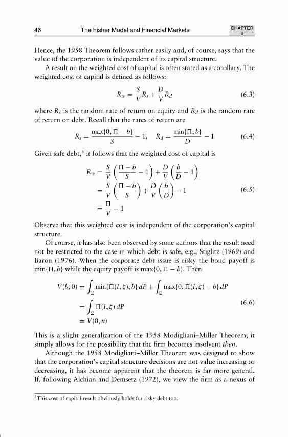
August 18, 2005 11:42 SPI-B312 The Fisher Model and Financial Markets (ED: Chean Chian) ch06
46 The Fisher Model and Financial Markets CHAPTER6
Hence, the 1958 Theorem follows rather easily and, of course, says that thevalue of the corporation is independent of its capital structure.
A result on the weighted cost of capital is often stated as a corollary. Theweighted cost of capital is defined as follows:
Rw = SV
Rs + DV
Rd (6.3)
where Rs is the random rate of return on equity and Rd is the random rateof return on debt. Recall that the rates of return are
Rs = max{0, � − b}S
− 1, Rd = min{�, b}D
− 1 (6.4)
Given safe debt,3 it follows that the weighted cost of capital is
Rw = SV
(� − b
S− 1
)+ D
V
(bD
− 1)
= SV
(� − b
S
)+ D
V
(bD
)− 1
= �
V− 1
(6.5)
Observe that this weighted cost is independent of the corporation’s capitalstructure.
Of course, it has also been observed by some authors that the result neednot be restricted to the case in which debt is safe, e.g., Stiglitz (1969) andBaron (1976). When the corporate debt issue is risky the bond payoff ismin{�, b} while the equity payoff is max{0, � − b}. Then
V(b, 0) =∫
�
min{�(I, ξ ), b} dP +∫
�
max{0, �(I, ξ ) − b} dP
=∫
�
�(I, ξ ) dP
= V(0, n)
(6.6)
This is a slight generalization of the 1958 Modigliani–Miller Theorem; itsimply allows for the possibility that the firm becomes insolvent then.
Although the 1958 Modigliani–Miller Theorem was designed to showthat the corporation’s capital structure decisions are not value increasing ordecreasing, it has become apparent that the theorem is far more general.If, following Alchian and Demsetz (1972), we view the firm as a nexus of
3This cost of capital result obviously holds for risky debt too.

August 18, 2005 11:42 SPI-B312 The Fisher Model and Financial Markets (ED: Chean Chian) ch06
CHAPTER6
Corporate Finance Theorems 47
contracts then the question of an optimal composition of contracts naturallyarises. The 1958 Theorem limits the contract set to debt and equity and saysthat the composition of the contract set is irrelevant. The theorem, however,generalizes quite easily to more complex contract sets and still provides anirrelevance result that says that the composition of the contract set is irrele-vant. For example, consider a futures contract. Let � denote unit payoff onthe stock index and let f denote the futures price. The payoff on the futuresposition is φ(f − �), where φ is the number of futures purchased. The cor-porate payoff is � + φ(f − �) and the value of the hedged firm is equal tothe value of the unhedged firm, i.e.,
S(0, n, φ) =∫
�
(�(I, ξ ) + φ(f − �)) dP
= S(0, n, 0) + φ
∫�
(f − �) dP
= S(0, n, 0)
(6.7)
This follows because the risk adjusted present value of the futures price equalsthe risk adjusted present value of the unit payoff. This line of analysis willbe pursued in the risk management chapter.
1961 Miller–Modigliani Theorem: If the financial markets are compet-itive, ceteris paribus, the value of the corporation paying dividends equalsthat of the corporation paying no dividends.
Holding the corporate investment decision fixed, the dividend policyquestion may be understood as the question of whether the corporationshould raise funds internally or externally. Equivalently, dividend policy maybe understood as the question of whether investors would prefer the corpo-ration to keep its earnings and invest them or pay them out now as divi-dends. In a competitive market system with no taxes, we show that the 1958Modigliani–Miller result on the irrelevance of the firm’s capital structuremay be combined with the 1961 Miller–Modigliani result on the irrelevanceof dividend policy, to show that the source and type of funds used to financean investment project have no effect on the value of the corporation.4
Consider introducing a dividend now. Let d denote the total number ofdollars in dividends paid by the firm now to holders of record in proportionto their ownership of the firm. Since we want to consider pre-dividend val-ues, suppose that the sequence of events is as follows: Firms announce theirdividend policies and trading occurs in the bond and stock markets; then
4Source refers to external versus internal funds while type refers to the characteristics of theissue, e.g., debt or equity.
August 18, 2005 11:42 SPI-B312 The Fisher Model and Financial Markets (ED: Chean Chian) ch06
48 The Fisher Model and Financial Markets CHAPTER6
dividends are paid and consumption now takes place. The financing and div-idend decisions may be represented by the triple (b, n, d), where b representsthe face value of a debt issue, n represents the number of new shares issued,and d represents the dividend paid now. Let S(b, 0, d) denote the stock mar-ket value of the firm now, given that the firm pays a dividend and issuesdebt to finance its investment. Similarly, let S(0, 0, 0) denote the stock mar-ket value of the firm which pays no dividend and finances its investment withretained earnings.5 Finally, let S(0, n, d) denote the stock market value of thefirm that pays a dividend and finances its investment by issuing new equity.Then it follows trivially that S(b, 0, d) = S(0, 0, 0) = S(0, n, d) − d, as thefollowing analysis shows.
Now, consider the dividend decision. Let the pair (π , �(I, ξ )) denote thefirm’s earnings now and then, respectively. Suppose the firm’s investmentdecision is fixed so that its earnings then are not affected by dividend policy.Further, suppose that π is sufficient to cover the firm’s investment expendi-ture now if it is retained, i.e., letting I denote the fixed investment expenditurenow, we suppose π − I = 0. If earnings now are not retained then the firmmust issue equity or debt to cover its fixed investment expenditure. If thefirm selects a dividend now of d > 0 and issues debt to finance its investmentthen the stock value is
So(b, 0, d) = d +∫
�
[�(I, ξ ) − b] dP
=∫
�
�(I, ξ ) dP
= So(0, 0, 0)
(6.8)
This result follows since the value of the debt issue equals the value of thedividend payment, i.e.,
D(b) =∫
�
b dP = I = π = d (6.9)
This result says that the stock value of the firm paying a dividend and raisingthe dollars needed for investment with a debt issue is the same as the stockvalue of the firm paying no dividend and raising all the dollars internally.Note that the stock market values here refer to both the total stock value
5In this section of the paper, we will assume that the firm has earnings now denoted by πf 0. Ofcourse, there is no uncertainty about the firm’s current earnings. Since the firm pays dividendsout of current earnings, this will allow us to specify a dividend now for the investors, in two ofthe three financing methods considered here.

August 18, 2005 11:42 SPI-B312 The Fisher Model and Financial Markets (ED: Chean Chian) ch06
CHAPTER6
Corporate Finance Theorems 49
and current shareholder value because there are no new equity holders; inthe next case the distinction becomes important. Suppose the firm pays adividend and issues new equity to finance the investment. Then the currentshareholder value is
So(0, n, d) = S(0, n, d) − Sn(0, n, d)
= d +∫
�
�(I, ξ ) dP − I
= So(0, 0, 0)
(6.10)
This result follows since the value of the new equity issue equals the value ofthe dividend payment, i.e.,
Sn(0, n, d) = I = π = d (6.11)
This result says that the current shareholder value of the firm paying a div-idend and raising the dollars needed for investment with a new equity issueis the same as the stock value of the firm paying no dividend and raisingall the dollars internally. Equations (6.8) and (6.10) suffice to demonstratethe 1961 Miller–Modigliani Theorem on the irrelevance of dividend policy.It may also be noted that the 1958 Modigliani–Miller Theorem follows asa corollary. Observe that the corporate value given the financing triple isV(b, n, d); then
V(b, 0, d) ≡ D(b) + S(b, 0, d)
= d +∫
�
�(I, ξ ) dP
= S(0, n, d)
= V(0, n, d)
(6.12)
Note that (6.12) holds dividend policy fixed and shows that the value of thelevered firm equals that of the unlevered firm.
1963 Modigliani–Miller Theorem: If the financial markets are competi-tive and corporations are taxed, ceteris paribus, the value of the levered firmequals that of the unlevered firm plus the value of the debt tax shield.
In this extension of the 1958 capital structure result, Modigliani andMiller consider an economy in which individual investors are not taxed butcorporations are taxed at a rate t. Since interest payments on the firm’s debtissue are deductible, the corporation can limit its tax payment to the Govern-ment by increasing the size of its debt issue and so reducing the corporation’staxable income. This motivates the 1963 Modigliani–Miller result which saysthat the value of the levered corporation equals the value of the unlevered

August 18, 2005 11:42 SPI-B312 The Fisher Model and Financial Markets (ED: Chean Chian) ch06
50 The Fisher Model and Financial Markets CHAPTER6
corporation plus the value of the corporate debt tax shelter. Of course, in itsstrictest form this result implicitly assumes that any redundant deductionscan be preserved without cost through merger, leasing, or other financialtransactions. Since the interest payments on debt are tax deductible we intro-duce coupon bearing bonds here and let r denote the coupon rate. Then thecorporation’s taxable income is � − rb where b is now the face value of thedebt instrument. Letting T denote the corporation’s tax liability, we have
T = t max{0, � − rb} (6.13)
The value of the tax liability in the absence of insolvency risk is∫�
t max{0, � − rb} dP = t∫
�
(� − rb) dP
= tV − trb
1 + r
(6.14)
For the unlevered firm, the right hand side of (6.14) reduces to tV . The returnto bondholders is
min{(1 + r)b, � − T} (6.15)
while the return to shareholders is
max{0, � − min{(1 + r)b, � − T} − T} (6.16)
Given no insolvency risk the returns to bondholders and shareholders are(1 + r)b and
� − (1 + r)b − t(� − rb) = (1 − t)� − (1 + r(1 − t))b (6.17)
respectively. Suppose the bond was issued at par so that∫�
dP = 11+r
6; thengiven no insolvency risk the value of the debt issue is
D =∫
�
(1 + r) b dP
= b(6.18)
and the levered value of the equity is S� where
S� =∫
�
((1 − t)� − (1 + r(1 − t))b) dP (6.19)
6The left hand side is the sum of the basis stock prices and is always equal the discount factorfor a safe asset that is shown on the right hand side; the only difference here is that the interestrate on the right hand side is also the coupon rate.

August 18, 2005 11:42 SPI-B312 The Fisher Model and Financial Markets (ED: Chean Chian) ch06
CHAPTER6
Corporate Finance Theorems 51
Hence, letting V� and Vu denote the levered and unlevered corporate values,respectively, the levered corporate value is
V� = D + S�
=∫
�
(1 + r)b dP +∫
�
((1 − t)� − (1 + r(1 − t))b) dP
=∫
�
((1 − t)� + trb) dP
= Vu + trb∫
�
dP
= Vu + trb
1 + r
= Vu + C
(6.20)
Figure 6.1 is a simple demonstration of the 1963 Theorem. It says that thevalue of the levered corporation is the risk adjusted present value of the aftertax cash flow or equivalently the value of the unlevered corporation plusthe present value of the debt tax shelter. The corporation can increase valueby levering up but as Figure 6.1 demonstrates, the corporation risks loosingtax credits if the leverage increases to a point at which the debt introducesinsolvency risk. The areas labeled T and C in Figure 6.1 represent the valueof the corporate tax liability and debt tax shelter, respectively. The figurealso makes it quite clear that the increase in corporate value is achieved byreducing the value of the tax liability. Hence, there is no change in value.There is only a redistribution of value.
Figure 6.1 The 1963 Miller–Modigliani Theorem.

August 18, 2005 11:42 SPI-B312 The Fisher Model and Financial Markets (ED: Chean Chian) ch06
52 The Fisher Model and Financial Markets CHAPTER6
1977 Miller Theorem: If the financial markets are competitive and bothcorporations and investors are taxed, the equilibrium value of the leveredfirm equals that of the unlevered firm.
Miller argued that, in an economy with investors in different personaltax brackets and with limitations on short selling, corporations will attemptto increase value by issuing bonds but the bond rate of interest will be drivenup to the point at which the net present value of the tax shelter is zero.Equivalently, he argued that, in such an economy, the value of the leveredfirm will equal the value of the unlevered firm. Miller demonstrated the resultunder certainty. Also see DeAngelo and Masulis (1980) and MacMinn andMartin (1988) for discussion.
1980 DeAngelo–Masulis Theorem: If the financial markets are compet-itive but corporations cannot protect tax credits and shields without cost,the equilibrium value of the levered firm equals that of the unlevered firmplus the values of the tax shields and credits; in some market equilibria thelevered value plus the shields and credits exceeds the unlevered value.
DeAngelo and Masulis demonstrated Miller’s result under uncertainty ina complete market model and then went on to show that, by modifying thetax treatment of corporations, an optimal capital structure can be determinedfor the firm. DeAngelo and Masulis, however, assumed that the total debtpayment could be deducted from corporate earnings in determining taxableincome.
Remarks
There are a few more classic theorems in corporate finance that are consideredin subsequent chapters. The risk-shifting or equivalently asset substitutionproblem will be considered in Chapter 7 while the pecking order theoremwill be considered in Chapter 8.
Suggested Problems
1. Suppose the levered firm does have some insolvency risk so that the returnsto bondholders and stockholders are as given in (6.15) and (6.16), respec-tively. Does a generalized version of the 1963 Theorem hold? Specify thelevered corporate value and discuss it.
2. Suppose investors have tax rates ti on the interest from corporate bondsthey may hold and that some investors have tax rates higher and lowerthan the corporate tax rate. Derive the supply and demand for bond funds.Use these functions to demonstrate the Miller 1977 Theorem.

August 18, 2005 11:42 SPI-B312 The Fisher Model and Financial Markets (ED: Chean Chian) ch07
Chapter 7Agency Problems
I n this chapter, two of the classic agency problems are considered. The firstis the risk-shifting or equivalently the asset substitution problem. It incor-
porates the simplest type of asymmetric information problem in the formof a hidden action taken by corporate management. The firm issues bondsto finance its investment in either one of two mutually exclusive projects.One of the projects is riskier than the other and the investors do not knowwhich project the firm will select. Hence, there is a hidden action. The riskierproject yields a smaller bondholder return. The investors must be able topredict which project the firm will select in order to value the bonds andthey are aware of the firm’s ability to shift risk to bondholders if the bondsare not appropriately valued. Given these circumstances there can be a con-flict between stockholders and bondholders with respect to project selection.Green (1984) considered a version of this problem and showed how convert-ible bonds could be used to solve the problem as will be done here.
The second agency problem is the under-investment problem. The classicstatement of the problem is that the firm is currently levered and is consid-ering financing for another project. Although the new financing is appropri-ately valued in financial markets, the benefits of the new project are sharedby both current stockholders and bondholders. Again, under these circum-stances there can be a conflict between stockholders and bondholders withrespect to the level of investment.
The Risk-Shifting Problem
Consider a corporation selecting between two mutually exclusive investmentprojects and financing the chosen project with debt. Both projects require
53

August 18, 2005 11:42 SPI-B312 The Fisher Model and Financial Markets (ED: Chean Chian) ch07
54 The Fisher Model and Financial Markets CHAPTER7
the same investment expenditure and one is riskier than the other in theRothschild–Stiglitz (1970) sense, i.e., one project has more weight in thetails of its return distribution. Since the investment is made subsequent toobtaining the necessary funds, bondholders do not observe the project choice.Under these circumstances a risk shifting problem may exist, since the cor-porate manager has the ability to devalue a corporate debt issue by selectingthe riskier project.
Consider the use of convertibles in resolving a conflict of interest problem.Corporate management can, for example, encounter a conflict of interests’problem in dealing with bondholders. Since the corporate manager representsthe interests of stockholders and bondholders, there is a potential for conflictbetween the manager and bondholders, or equivalently, between the managerand the bondholders’ trustee. This will be the case if it is possible for themanager to take actions that benefit one group and are detrimental to theother. If the bonds represent secured debt then there is no conflict. If not,then an agency problem may exist.
The agency relationship can be thought of as a contract between theprincipal (i.e., the bondholders’ trustee)1 and an agent (i.e., the corporatemanager). The agent acts on behalf of the principal. The contract specifiesthe bounds on the actions that may be taken by the agent. If the contractcovers all possible contingencies then there is no real delegation of authorityand so no agency problem. If the contract is incomplete so that the agent hassome discretion in the selection of actions then there is at least the potentialfor a conflict of interests. The conflict occurs because both the principal andthe agent behave in accordance with their own self interests. The principalcan limit the divergence of interests by providing provisions in the contractthat give the agent the appropriate incentives to act in the principal’s interest;in addition, the principal can monitor the activity of the agent. It is not usuallypossible, however, to specify the contract in a way that completely eliminatesthe conflict of interests’ problem. Hence, it may be the case that there is adifference between the action taken by the agent and the action that is in
1The legal trustee for the bondholders may be treated as the single principal. It should be addedthat the trustee acts on behalf of the bondholders. The trustee’s problem is the selection ofbond covenants that limit the divergence of interests between corporate management and thebondholders. In general, the trustee may have a problem in selecting covenants that provide asolution to the conflict because of the different risk aversion measures of the bondholders. Inthe case considered here, however, the bondholders will unanimously support a covenant thatprovides management with the incentive to maximize the risk adjusted net present value of thecorporation. It should also be noted that in general there may be an agency problem betweenthe trustee and bondholders (i.e., between the agent and the principals). In the case consideredhere that problem does not arise because of the unanimity.

August 18, 2005 11:42 SPI-B312 The Fisher Model and Financial Markets (ED: Chean Chian) ch07
CHAPTER7
Agency Problems 55
the best interests of the principal. The agency cost is defined, by Jensen andMeckling (1976), as the sum of the monitoring expenditures of the principal,the bonding expenditures of the agent, and the residual loss; this residual lossis the loss in the market value of the corporation.2
The agency problem we consider here is encountered by the corporationin selecting among mutually exclusive investment projects. Jensen and Smithnoted that
“. . . the value of the stockholders’ equity rises and the value of thebondholders’ claim is reduced when the firm substitutes high-riskfor low-risk projects.”3
Of course, bondholders are aware of this possibility, i.e., this attempt toshift risk, and so it is reflected in a lower value for the corporation’s debt issue.We want to show that it is possible to construct a convertible bond packagethat will reduce or eliminate the risk-shifting incentive and so the agency costof debt. The first step in this process, however, is the demonstration of theagency problem and its cost.
The existence issue
In order to demonstrate the agency problem, suppose the corporation is con-sidering two mutually exclusive investment projects. Call them projects oneand two. Let I1 = I2 ≡ I denote the dollar cost of the two projects and let�1 and �2 denote the random project earnings.4 Suppose project earningsare positive for all states. Suppose project two is riskier than project one,in the Rothschild–Stiglitz sense. In particular, let �2 be a mean-preservingspread of �1, as shown in Figure 7.1, i.e., �2 = (1 + δ)�1 − δE�1,
2Jensen, M. and W. Meckling (1976). “Theory of the Firm: Managerial Behavior Agency Costsand Ownership Structure.” Journal of Financial Economics 3: 305–360, also define the residualloss as the dollar equivalent of the loss in expected utility experienced by the principal. Althoughthis notion of residual loss is measurable for a particular principal, this definition poses problemswhen a trustee represents many principals because the residual loss of any bondholder willdepend on the bondholder’s measure of risk aversion and on the proportion of the contractowned.3See Jensen, M. and C. Smith (1985). “Stockholder, Manager, and Creditor Interests:Applications of Agency Theory.” Recent Advances in Corporate Finance. E. Altman andM. Subrahmanyam, eds. Richard D. Irwin. Also see Green, R.C. (1984). “Investment Incen-tives, Debt, and Warrants.” Journal of Financial Economics 13: 115–136 and Smith, C. andJ. Warner (1979). “On Financial Contracting: An Analysis of Bond Covenants.” Journal ofFinancial Economics 7: 117–161, for similar statements.4For notational simplicity, we drop the subscript indicating the corporation and replace it witha subscript indicating the project.

August 18, 2005 11:42 SPI-B312 The Fisher Model and Financial Markets (ED: Chean Chian) ch07
56 The Fisher Model and Financial Markets CHAPTER7
Figure 7.1 Project risk.
Figure 7.2 Debt devaluation.
δ > 0.5 Then µ2 = E�2 = E�1 = µ1 and �2 has more weight in thetails of its distribution, as may be seen in Figure 7.1.
In this context, consider the statement by Jensen and Smith. Supposebondholders believe that the firm will select project one and value the bondissue accordingly. This means, of course, that the promised payment b onthe debt is selected so that the value of the debt issue raises the amountnecessary for the investment of I dollars, i.e., D1(b) = I. Next, suppose thefirm switches to project two and note that D2(b) < D1(b), or equivalently,investors would not have provided the funds necessary for the investmenthad they known that project two would be selected. If the firm switches thenthe value of the bondholders’ claim is reduced by the amount D1 − D2, asshown in Figure 7.2.
5The state space is still assumed to be finite but it is easier to see the mean-preserving spreadwhen � is drawn as a continuous function of ω.

August 18, 2005 11:42 SPI-B312 The Fisher Model and Financial Markets (ED: Chean Chian) ch07
CHAPTER7
Agency Problems 57
Hence, there are circumstances under which it is not rational for thebondholders to believe any claim made by the firm that project one willbe selected. Rational bondholders will protect their interests by consideringwhat project will be selected by a management that acts in the best interestsof its shareholders.
The first claim we want to make is that there exists a promised paymentlevel b∗ such that S2(b) > S1(b) for b > b∗ and S2(b) < S1(b) for b < b∗.This may be done simply by showing that in the unlevered case S1(0) = V1 >
V2 = S2(0) and in the sufficiently highly levered case S2(b) > S1(b). Then theIntermediate Value Theorem yields the existence of a b∗.
Following the outlined procedure, first, we want to show that if the cor-poration is unlevered and if project two is riskier than project one, thenS1(0) = V1 > V2 = S2(0). Note that the difference in value is
V1 − V2 =∫
�
�1(ξ ) dP −∫
�
�2(ξ ) dP
=∫
�
(�1(ξ ) − �2(ξ )) dP
= δ
∫�
(µ − �1(ξ )) dP
= δ(pµ − V1)> 0
(7.1)
where p is the sum of the basis stock prices. The inequality follows sincepµ1 > V1, i.e., the present value of a safe asset with the same expectedpayoff as the project is greater than the risk adjusted present value of theproject.6
Second, we want to show that in the highly levered case the stock marketvalue of the riskier project is greater. To do this, simply note that for bsufficiently large max{0, �2 − b} ≥ max{0, �1 − b} for all ξ ∈ � and strictlygreater for some ξ , as shown in Figure 7.3. It follows trivially that
S2(b) =∫
�
max{0, �2(ξ ) − b} dP
>
∫�
max{0, �1(ξ ) − b} dP (7.2)
= S1(b)
Then continuity completes the proof and we have the existence of a promisedpayment level b∗ such that S2(b) > S1(b) for b > b∗ and S2(b) < S1(b) for
6See MacMinn, R.D. (1987). “Lecture Notes on the Risk-Shifting Problem” for a demonstrationof this result.

August 18, 2005 11:42 SPI-B312 The Fisher Model and Financial Markets (ED: Chean Chian) ch07
58 The Fisher Model and Financial Markets CHAPTER7
Figure 7.3 Levered stock payoffs.
b < b∗. Therefore, in the absence of any mechanism to avoid the agencyproblem, the corporation with a promised payment b > b∗ has an incentiveto accept the riskier project.
The agency cost
In its simplest form the agency cost of debt is
V1 − V2 =∫
�
(�1 − �2) dP > 0 (7.3)
when the agency problem exists. Actually, claiming that the corporation hasan incentive to accept the riskier project is deceptive. Suppose the corporationmust make a promised repayment of b1 dollars in order to finance projectone, i.e., D1(b1) = I, given that bondholders believe that project one will beselected. However, if b1 > b∗ then the corporate management has a moralhazard problem since S2(b1) > S1(b1). Rational bondholders understand thisconflict of interest problem and will value the bond issue as if project twowill be selected. Since D2(b1) < I, it follows that the promised repaymentmust be increased to b2 > b1 so that D2(b2) = I. The equity is appropriatelypriced as S2(b2) but the agency cost is not directly reflected in this expression.It is possible to rewrite the stock market value S2(b2) to reflect the agencycost. To do this, note that the promised payment b2 must be selected so that
S2(b1) − S2(b2) = D1(b1) − D2(b1)7 (7.4)
7This is equivalent to S2(b1) = S2(b2) + D1(b1) − D2(b1) which simply says that if the bond-holders believe that the firm will select project one and the firm selects project two, then thestock market value of project two is its true value plus the devaluation of the bond issue.

August 18, 2005 11:42 SPI-B312 The Fisher Model and Financial Markets (ED: Chean Chian) ch07
CHAPTER7
Agency Problems 59
Figure 7.4 Difference in promised payment.
These differences in value are shown in Figure 7.4. Note that S2(b2) may beequivalently expressed as
S2(b2) = S2(b1) − (D1(b1) − D2(b1)) (7.5)
Also note that
V1 − V2 = D1(b1) − D2(b1) + S1(b1) − S2(b1)8 (7.6)
or equivalently,
S2(b1) = S1(b1) + (D1(b1) − D2(b1)) − (V1 − V2) (7.7)
Then substituting (7.5) into (7.7) and simplifying yields
S2(b2) = S1(b1) − (V1 − V2) (7.8)
Hence, the stock market value of project two equals that of project oneminus the agency cost of the bond issue. Observe that S2(b2) < S1(b1). Thismakes it clear that it would be in the best interests of management to con-vince bondholders that project one will be selected. Because of the moralhazard problem, however, the straight bond contract cannot be used to con-vince them. With a straight bond contract, the bondholders must expect thedevaluation. What is more, at b2, S2(b2) > S1(b2) and the higher promisedrepayment locks management into the choice of project two.
8This follows by the 1958 Modigliani–Miller Theorem.

August 18, 2005 11:42 SPI-B312 The Fisher Model and Financial Markets (ED: Chean Chian) ch07
60 The Fisher Model and Financial Markets CHAPTER7
The convertible bond solution
Next, consider the value of convertible bonds. Suppose each bond is issuedwith a call option which gives its owner the right to exchange a bond forθ = γ (N + n)/b shares of stock, where n is the number of new shares whichmust be issued if the bonds are converted. Note that a convertible bond issimply a bond with an attached call option. Also note that γ is the fraction ofthe firm’s equity payoff that goes to bondholders in the event that the optionis exercised. As has been shown, the payoff on the convertible bond issue ismin{�, b} + max{0, γ� − b}, where b is the exercise value of the call optionissue. Then it follows easily that the market value of the convertible bondissue is
D(b, γ ) =∫
�
min{�, b
}dP +
∫�
max{0, γ� − b
}dP
= D(b) + C(b, γ )(7.9)
Similarly, the value of the stock is
S(b, γ ) =∫
�
max{0, � − b
}dP −
∫�
max{0, γ� − b
}dP
=∫
�\B
(� − b
)dP −
∫E
(γ� − b
)dP (7.10)
= S(b) − C(b, γ )
i.e., the stock market value of the firm with convertible debt is equivalentto the stock market value of the firm with the simple debt contract minusthe value of the option. In the second expression for stock value, B is thebankruptcy event and E is the exercise event. Note that the bankruptcy eventis B = {ξ ∈ �|�(ξ ) < b} = [0, δ) and the exercise event is E = {ξ ∈�|γ�(ξ ) ≥ b} = [ζ , ω], where � = [0, ω], as shown in Figure 7.5.
It may be noted that since the corporate value is not affected by theintroduction of an option to convert, it follows that the option reduces thestock market value.
Now, consider how management can construct a convertible issue thatwill convince the bondholders that project one will be selected. In fact,suppose management constructs the package to convince bondholders thatproject one will be selected and to maximize the stock market value of thecorporation by eliminating the agency cost of the bond issue. Suppose man-agement selects the provisions of the bond issue, i.e., (b, γ ), so that the projectis financed and so that C2 −C1 > D1 −D2. The latter is simply the conditionthat the difference in the value of the call options exceed the difference in
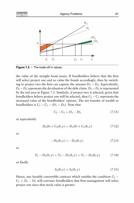
August 18, 2005 11:42 SPI-B312 The Fisher Model and Financial Markets (ED: Chean Chian) ch07
CHAPTER7
Agency Problems 61
Figure 7.5 The trade-off in values.
the value of the straight bond issues. If bondholders believe that the firmwill select project one and so value the bonds accordingly, then by switch-ing to project two the firm can capture the amount D1 − D2. Equivalently,D1 −D2 represents the devaluation of the debt claim. D1 −D2 is representedby the red area in Figure 7.5. Similarly, if project two is selected, given thatbondholders believe project one will be selected, then C2 − C1 represents theincreased value of the bondholders’ options. The net transfer of wealth tobondholders is C2 − C1 − (D1 − D2). Note that
C2 − C1 > D1 − D2 (7.11)
or equivalently
D2(b) + C2(b, γ ) > D1(b) + C1(b, γ ) (7.12)
or
−D2(b, γ ) < −D1(b, γ ) (7.13)
or
V2 − D2(b, γ ) < V2 − D1(b, γ ) < V1 − D1(b, γ ) (7.14)
or finally
S2(b, γ ) < S1(b, γ ) (7.15)
Hence, any feasible convertible contract which satisfies the condition C2 −C1 > D1 − D2 will convince bondholders that firm management will selectproject one since that stock value is greater.

August 18, 2005 11:42 SPI-B312 The Fisher Model and Financial Markets (ED: Chean Chian) ch07
62 The Fisher Model and Financial Markets CHAPTER7
It only remains to be shown that this technique of issuing convertiblebonds to address the agency problem eliminates the problem and the cost.Recall that S2(b2) = S1(b1) − (V1 − V2). By the 1958 Modigliani–MillerTheorem and the financing conditions, S1(b, γ ) = S1(b1). It follows thatS1(b, γ ) − S2(b2) = V1 − V2 > 0. Therefore, the agency cost is eliminatedand the manager prefers the convertible debt issue to a straight debt issue.
The solution set
It is possible to solve the risk-shifting problem with a convertible bond issuebut how many convertible bond contracts solve the problem and finance theinvestment? The set of feasible contracts is shown in Figure 7.6. The set offeasible contract is, of course, the set of convertible bonds that finances theinvestment. The solution set is a subset of this space and the solution set sat-isfies the following two conditions: (i) D1(b, γ ) = I; (ii) D2(b, γ ) > D1(b, γ ).The first condition is the financing condition while the second condition isequivalent to the condition that stock value is greater given the selection ofproject one.
The conditions implicitly define functional relationships between the con-tract parameters. The financing constraint yields a function γ = h(b); the(b, γ ) pairs on h satisfy the financing condition. It may be noted that h isa decreasing function since a larger promised payment on the bond allowsa smaller promised equity stake in the event that the bond is converted. Todemonstrate this relationship, observe that
h′ = −∂D1∂b
∂D1∂γ
≤ 0 (7.16)
Figure 7.6 The solution set.
August 18, 2005 11:42 SPI-B312 The Fisher Model and Financial Markets (ED: Chean Chian) ch07
CHAPTER7
Agency Problems 63
since the bond value is increasing in both parameter values, i.e.,
∂D1
∂b=
∫ ζ1
δ1
dP ≥ 0 and∂D1
∂γ=
∫ x
ζ1
�1dP ≥ 0 (7.17)
Next, consider the set of parameters (b, γ ) such that the convertible bondvalues are equal, i.e., D1(b, γ ) = D2(b, γ ); suppose this equality implicitlyspecifies the function γ = g(b). Then
g′ = −∂D1∂b − ∂D2
∂b∂D1∂γ
− ∂D2∂γ
> 0 (7.18)
since we may observe that
∂D1
∂b− ∂D2
∂b=
∫ ζ1
δ1
dP −∫ ζ2
δ2
dP
=∫ δ2
δ1
dP +∫ ζ1
ζ2
dP (7.19)
> 0
and
∂D1
∂γ− ∂D2
∂γ=
∫ ω
ζ1
�1dP −∫ ω
ζ2
�2dP
= −∫ ζ1
ζ2
�2dP −∫ ω
ζ1
(�2 − �1) dP (7.20)
< 0
The solution set consists of all the contracts (b, γ ) on h above g.
The Under-investment Problem
The second of two classic agency problems considered here is the under-investment problem. Notice that acting in the interests of the old shareholdersgenerates the under-investment problem. This problem has been describedas limiting the investment expenditure because the additional returns accrueto bondholders as well as stockholders. This problem can be associated withat least two possible scenarios. First, if the firm is already levered enoughto make the probability of insolvency positive then the under-investmentproblem can occur; second, if information concerning the corporate invest-ment opportunity is hidden then the problem can also occur. The first sce-nario will be considered here briefly and the second will be considered inmore detail in the next chapter.

August 18, 2005 11:42 SPI-B312 The Fisher Model and Financial Markets (ED: Chean Chian) ch07
64 The Fisher Model and Financial Markets CHAPTER7
The corporate manager, acting in the interests of the old shareholders,may not invest in positive net present value projects or may under-invest in theprojects. This problem occurs because the returns accrue in part to existingbondholders as well as to stockholders. Jensen and Smith observed that
“. . . when a substantial portion of the value of the firm is com-posed of future investment opportunities, a firm with outstand-ing risky bonds can have incentives to reject positive net presentvalue projects if the benefit from accepting the project accrues to thebondholders.”9
The incentive need not be so extreme as to cause the manager to reject aproject; the manager may under-invest by limiting the size of the project. Wewill identify the problem in a somewhat general setting without yet attempt-ing to form a solution. One solution to the under-investment problem doesexist in the literature, e.g., see Mayers and Smith (1987) and Garven andMacMinn (1993). The solution is provided in an insurance model and thereit alters incentives by bundling insurance with a bond contract or equiva-lently attaching a covenant to the bond instrument that requires insuranceand ensures that the net present value of the investment goes to shareholders.
The existence issue
To demonstrate the existence of the problem, suppose the corporate payoffthen is �(I, ξ )10 and that the firm has previously issued zero coupon bondswith a promised payment of bo dollars and is now going to make a promisedpayment of bn dollars to raise I dollars for an additional project. Supposethat the probability of insolvency is positive, i.e., P{�(0, ξ ) < bo} > 0. Alsosuppose that the investment increases the corporate payoff so that
∂�
∂I> 0 and
∂2�
∂I2< 0 for all ξ ∈ � (7.21)
Suppose that the firm issues new debt with a promised payment bn to financethe investment of I dollars now; finally suppose for simplicity that the newdebt is subordinate to the old. The manager paid in salary and corporate
9See Jensen, M. and C. Smith (1985). “Stockholder, Manager, and Creditor Interests:Applications of Agency Theory”. Recent Advances in Corporate Finance. E. Altman andM. Subrahmanyam, eds. Richard D. Irwin, Bodie, Z. and R. Taggart (1978). “Future Invest-ment Opportunities and the Value of the Call Provision on a Bond.” Journal of Finance 33:1187–1200, Myers, S. C. (1977). “The Determinants of Corporate Borrowing.” Journal ofFinancial Economics 5: 147–175. Smith, C. and J. Warner (1979). “On Financial Contracting:An Analysis of Bond Covenants.” Journal of Financial Economics 7: 117–161.10The payoff could have been divided into a payoff for previous investments and another forthe current investment but that would complicate the notation without adding insight.

August 18, 2005 11:42 SPI-B312 The Fisher Model and Financial Markets (ED: Chean Chian) ch07
CHAPTER7
Agency Problems 65
stock will make decisions to solve the following constrained maximizationproblem:
maximize So(I)
subject to Dn(bn) = I(7.22)
where, letting δ be implicitly defined by �(I, δ) − bo − bn = 0,
So(I) =∫
�
max{0, �(I, ξ ) − bo − bn} dP
=∫ ω
δ
(�(I, ξ ) − bo − bn) dP
(7.23)
and, letting δo define the boundary of the insolvency event given no newinvestment,
Dn(bn) =∫
�
min{max
{0, �(I, ξ ) − bo} , bn} dP
=∫ δ
0max
{0, �(I, ξ ) − bo} dP +
∫ ω
δ
bndP (7.24)
=∫ δ
δo
(�(I, ξ ) − bo) dP +
∫ ω
δ
bndP
Let bn(I) be the required promised payment on new debt required to satisfythe financing condition Dn(bn) = I. Note that
dbn
dI= 1∫ ω
δdP
11 (7.25)
Now the unconstrained maximization problem for the firm with debt over-hang is
maximize So(I) (7.26)
where
So(I) =∫ ω
δ
(�(I, ξ ) − bo − bn(I)
)dP (7.27)
11Observe that
∂Dn
∂bn = (�(I, δ) − bo)
p(δ)∂δ
∂bn +∫ ω
δ
dP − bnp(δ)∂δ
∂bn =∫ ω
δ
dP
and sodbn
dI= 1
∂Dn
∂bn
= 1∫ ω
δdP
.

August 18, 2005 11:42 SPI-B312 The Fisher Model and Financial Markets (ED: Chean Chian) ch07
66 The Fisher Model and Financial Markets CHAPTER7
and the first order condition is
dSo
dI=
∫ ω
δ
(D1�(I, ξ ) − dbn
dI
)dP
=∫ ω
δ
D1�(I, ξ ) dP − dbn
dI
∫ ω
δ
dP
=∫ ω
δ
D1�(I, ξ ) dP − 1
= 0
(7.28)
where the third equality in (7.28) follows by (7.25), or equivalently,∫ ω
δ
D1�(I, ξ ) dP = 1 (7.29)
The left hand side of (7.29) is the marginal benefit of the investment for theshareholders while the right hand side is the marginal cost. If there is nopositive probability of insolvency then the condition becomes∫ ω
0D1�(I, ξ ) dP = 1 (7.30)
If we let Iv satisfy (7.30) and Is satisfy (7.29) in the debt over-hang case, it isapparent that we have Is < Iv or equivalently the under-investment problemexists.
Remarks
The risk-shifting and under-investment problems are quite well known infinance. The risk-shifting problem has received a lot of attention and thereare well known and costless solutions, e.g., see Green (1984), and MacMinn(1987, 1993). The under-investment problem takes two forms, i.e., with andwithout asymmetric information. Debt over-hang yields the under-investmentproblem with symmetric information and has received less attention than itsasymmetric cousin. Indeed there only seems to be one solution to one specialcase of the debt over-hang version of the under-investment problem, e.g., seeMayers and Smith (1987) and Garven and MacMinn (1993). The secondversion of the under-investment problem is considered in the next chapter.
Suggested Problems
1. Show how to solve the risk-shifting problem with a bond-warrantpackage.
2. Design a contracting scheme to solve the debt over-hang version of theunder-investment problem.

August 18, 2005 11:42 SPI-B312 The Fisher Model and Financial Markets (ED: Chean Chian) ch08
Chapter 8Information Problems:
Hidden Knowledge
S ince investors must sometimes contend with incomplete information,the next logical step in describing financial markets entails the introduc-
tion of asymmetric information. Of course, asymmetric information charac-terized the risk shifting problem describe in the last chapter. The informationproblem there, however, was due to a hidden action and that action could notonly be changed but also rationally predicted by the other parties to the finan-cial transaction. The information problem addressed here can be describedas hidden knowledge and by that we mean that some market agents possessknowledge about the quality of an asset or project and that quality cannotbe altered. Myers and Majluf (1984) considered this hidden knowledge andshowed1 that the hidden knowledge motivates an under-investment prob-lem and can lead to a preference for debt over equity in financing. The latterpreference has become known as the pecking order theorem. Like Myers andMajluf, it is supposed here that the information cannot be revealed by the
1The Myers–Majluf model is different in some respects. The managers there know the projectpayoff with certainty and all market agents are risk neutral. While neither assumption is main-tained here, the results described by Myers and Majluf are robust to the model here.
67

August 18, 2005 11:42 SPI-B312 The Fisher Model and Financial Markets (ED: Chean Chian) ch08
68 The Fisher Model and Financial Markets CHAPTER8
choice of the financing scheme.2 How does the manager who possesses thehidden knowledge make decisions on corporate account? What impact doeshidden knowledge have on the choice of investment level and on the capitalstructure? These questions are addressed here.
If some market participants have access to knowledge that others donot, then it becomes necessary to differentiate between those that do andthose that do not have the knowledge. Here we will refer to market agentsas insiders and outsiders to describe those who possess and those who donot possess the knowledge, respectively. For simplicity, we suppose that theinsiders possess knowledge about the return on their corporation’s invest-ment project; that knowledge is hidden from the outsiders. While the cor-porate management may change the scale of the investment project, thequality of the project is given. The purpose of this chapter is to inves-tigate the implication that the hidden knowledge has for financing andinvestment decisions in a setting where all market agents, i.e., insiders andoutsiders are risk averse and the corporate objective function is endogenouslyderived.
As in the previous chapters, consider a competitive economy operat-ing between the dates now and then. All decisions are made now andall payoffs on those decisions are received then. Here, however, supposethe hidden knowledge exists in one industry where the corporations haveeither a good or less good investment opportunity. Suppose that tradingin financial markets occurs in basis and corporate assets. Finally, supposethat the information possessed by market participants is complete withrespect to all the financial markets assets except those of the industry underconsideration.
2There is also a literature on signaling hidden knowledge and is motivated by the notion thata financial contract can be structured that reveals the hidden knowledge to the market par-ticipants. The signaling notion is intriguing but goes beyond the scope of this work; a fewexamples of that literature are the following: Bhattacharya, S. (1980). “Nondissipative Sig-naling Structures and Dividend Policy. Quarterly Journal of Economics 95(1): 1–24, Riley,J. G. (1985). “Competition with Hidden Knowledge.” Journal of Political Economy 93(5):958–976, Brennan, M. and A. Kraus (1987). “Efficient Financing under Asymmetric Informa-tion.” Journal of Finance XLII(5): 1225–1243, Noe, T. (1988). “Capital Structure and Signal-ing Game Equilibria.” Review of Financial Studies 1: 331–356, Allen, F. and G. R. Faulhaber(1989). “Signaling by Underpricing in the IPO Market.” Journal of Financial Economics 23(2):303–323, Glazer, J. and R. Israel (1990). “Managerial Incentives and Financial Signaling inProduct Market Competition.” International Journal of Industrial Organization 8(2): 271–280,McNichols, M. and A. Dravid (1990). “Stock Dividends, Stock Splits, and Signaling.” Journalof Finance 45(3): 857–879, Sobel, J. et al. (1990). “Fixed-Equilibrium Rationalizability in Sig-naling Games.” Journal of Economic Theory 52(2): 304–331.

August 18, 2005 11:42 SPI-B312 The Fisher Model and Financial Markets (ED: Chean Chian) ch08
CHAPTER8
Information Problems: Hidden Knowledge 69
Outsiders
Suppose the financial markets for the assets of corporations in industry F arecharacterized by hidden knowledge. The knowledge that is hidden specifiesthe firm’s investment opportunity. Suppose there are two types of investmentopportunities and so two types of firms in this industry. Let �2(ξ ) > �1(ξ ),for all ξ ∈ �.3 Firm insiders have complete information, ex ante, concerningthe corporate payoff functions, individual investors or equivalently outsidersdo not. The investor purchasing an asset from a firm in this industry onlyknows that if state of nature ξ is realized, then the corporate payoff will be�1(ξ ) with probability 1 − θ or �2(ξ ) with probability θ ; θ is the proportionof firms in the industry that are type two, or equivalently, the probability ofrandomly selecting a type two firm. Also suppose that the investors know theproportion θ . It follows that the investors know the average industry payoff,i.e., �a(ξ ) = (1 − θ )�1(ξ ) + θ�2(ξ ).
When an investor purchases an asset from a firm in industry F, the payoffon the asset depends on the state of nature and the firm’s type. Since the typeis hidden knowledge, it introduces an additional source of risk. The addi-tional risk can be handled in a number of ways. First, although the financialcontracts sold by firms in industry F are no longer homogeneous, investorscan produce a homogenized asset by purchasing an equal proportion of eachfirm’s assets. Then the payoff on the portfolio is �a in each state of natureξ ∈ �. This eliminates the additional source of risk. In the absence of ascreening or signaling mechanism, investors will value firms in this industryon the basis of the average industry payoff and so the value of a firm is Va,where Va denotes corporate value from the outsiders’ perspective. Conse-quently, it also follows that the type one firms are over-valued and the typetwo firms are under-valued in a pooling equilibrium.
Unlevered case
If the corporations in the industry are unlevered then Figure 8.1 shows thecorporate value. The stock market value from the outsider’s perspective is
Sa =∫
�
�a(ξ ) dP
=∫
�
((1 − θ )�1(ξ ) + θ�2(ξ )) dP
= (1 − θ ) S1 + θ S2
(8.1)
3The terms type two and one are used synonymously with high and low investment opportunity,respectively. The inequality conditions guarantee that the random payoff of the high quality firmstochastically dominates that of the low quality firm in the first order sense.

August 18, 2005 11:42 SPI-B312 The Fisher Model and Financial Markets (ED: Chean Chian) ch08
70 The Fisher Model and Financial Markets CHAPTER8
Figure 8.1 Outsiders and value.
Suppose that the unlevered firm has previously issued N shares to the pub-lic and m shares to the manager. In addition, the firm issues na sharesnow to finance an investment of I dollars. na represents the number ofshares that must be issued in the presence of the hidden knowledge and willexceed the number n2 that would have to be issued for the same invest-ment in the absence of the hidden knowledge. The stock market valueof the new issue of stock from the insiders’ perspective is Sn
2(I, na) whileit is Sn
a (I, na) from the hedged outsiders’ perspective. There is some dilu-tion in the value of the current shareholders’ stake in the type two corpo-rations as represented by the red area in Figure 8.1. The agency cost ofthe new equity issue by type two corporations may be characterized as ce
a
where
cea = Sn
2(I, na) − Sna (I, na)
= na
N + na + m(S2 − Sa)
> 0
(8.2)
The agency cost due to the hidden knowledge is the red area depicted inFigure 8.1; it is also a fraction of the under-valuation of the type two firmand depicted as the green area in Figure 8.1.

August 18, 2005 11:42 SPI-B312 The Fisher Model and Financial Markets (ED: Chean Chian) ch08
CHAPTER8
Information Problems: Hidden Knowledge 71
Levered case
The capital structure of type two firms determines how the under-valuationis distributed across its assets. Consider a zero coupon bond issue with apromised payment then of b dollars. Let D2 and Da represent the bondvalue from the perspective of insiders and outsiders, respectively. Let δ1 andδ2 denote the boundaries of the solvency events for the type one and twolevered firms respectively. The fully hedged payoff to a risky bond issue bya type two corporation is
θ�2 + (1 − θ )�1 if ξ ≤ δ2
θb + (1 − θ )�1 if δ2 < ξ < δ1
b if ξ ≥ δ1
and so the bond value from the outsiders’ perspective is Da where
Da =∫ δ2
0�a dP +
∫ δ1
δ2
[θb + (1 − θ )�1] dP +∫ ω
δ1
b dP (8.3)
Since the levered value given the hidden knowledge is
D2 =∫ δ2
0�2 dP +
∫ ω
δ2
b dP (8.4)
it follows that the extent of the under-valuation of a type two firm’s debt is
D2 − Da =∫ δ2
0(�2 − �a) dP +
∫ δ1
δ2
[b − (θb + (1 − θ )�1)
]dP (8.5)
This is also the agency cost of the debt issue, i.e., cda = D2 − Da shown in
Figure 8.2.Similarly, let S2 and Sa represent the stock market value of a type two
firm from the perspective of insiders and outsiders, respectively. The payoffof fully hedged stockholders is
0 if ξ ≤ δ2
θ(�2 − b) if δ2 < ξ < δ1
�a − b if ξ ≥ δ1
The outsider stock value is Sa where
Sa =∫ δ1
δ2
θ(�2 − b) dP +∫ ω
δ1
(�a − b) dP (8.6)

August 18, 2005 11:42 SPI-B312 The Fisher Model and Financial Markets (ED: Chean Chian) ch08
72 The Fisher Model and Financial Markets CHAPTER8
Figure 8.2 Hidden knowledge and the agency cost of debt.
Figure 8.3 Hidden knowledge and levered values.
The outsider equity value is shown in Figure 8.3. Then, the extent of theunder-valuation of a type two firm’s equity is
S2 − Sa =∫ δ1
δ2
(1 − θ )(�2 − b) dP +∫ ω
δ1
(�2 − �a) dP ≥ 0
These results present corporate management with adverse incentives. Theadverse incentives become evident once the corporate manager’s objectivefunction is identified. If the manager cannot trade on the hidden knowledgethen the self interested corporate manager will make investment and financ-ing decisions to maximize her own stake in the corporation. The manager

August 18, 2005 11:42 SPI-B312 The Fisher Model and Financial Markets (ED: Chean Chian) ch08
CHAPTER8
Information Problems: Hidden Knowledge 73
makes decisions to maximize So2 and that current shareholder value can also
be represented as V2 − I − ca, where V2 is the corporate value of the highquality firm given insider information, I is the dollar amount raised fromoutsiders, and ca is the agency cost of outside finance.4 Hence, as Myersand Majluf noted, there are circumstances under which the firm will rejectpositive net present value projects, i.e., if V2 − I < ca.5 More generally, thefirm may simply invest less than the amount that maximizes the risk adjustednet present value of the corporation. This is one form that the adverse selec-tion problem can take. Even if the adverse selection problem is not severeenough to cause the firm to reject the project, i.e., V2 − I > ca, the hid-den knowledge still has an impact because the manager selects the financingmethod which minimizes the agency cost. This contract selection is impor-tant because, if the high quality firm cannot provide outsiders with credibleinformation about its quality, then the appropriate selection of a contract isthe only means the firm has available to mitigate the effects of the adverseselection problem.
Insiders
The hidden knowledge yields an adverse selection problem for corporatemanagers in the industry. The hidden knowledge generally makes it morecostly for the type two firms to issue some financial contracts. The kind offinancial instrument the firm chooses to issue becomes relevant in this settingbecause not all instruments yield the same agency cost. For example, Myersand Majluf demonstrated that a safe debt issue eliminates the agency cost ofoutside finance and so is preferred to an equity issue. This hidden knowledgealso affects the manager’s behavior on personal account because the type twomanagers cannot borrow against the full value of her equity stake in the cor-poration. This manager also knows that there will be a capital gain when thehidden knowledge becomes public and so the information affects the portfo-lio decision, e.g., fewer basis assets need to be purchased for those states inwhich the manager knows there will be a capital gain. It is assumed here thatthe manager cannot trade on inside information and that the manager’s port-folio decision is a hidden action. Both types of decisions on personal account
4See the analysis in the next section to confirm these claims.5There are significant differences between this model and that of Myers and Majluf but some oftheir conclusions are sufficiently robust to apply in the context of this model. Unlike this model,Myers and Majluf did not allow for risk aversion and the corporate manager was assumed toknow which of two states of nature would occur then.

August 18, 2005 11:42 SPI-B312 The Fisher Model and Financial Markets (ED: Chean Chian) ch08
74 The Fisher Model and Financial Markets CHAPTER8
have the potential to reveal information to outsiders.6 Less than completerevelation of the manager’s portfolio decision does not necessarily eliminatethe hidden knowledge problem, e.g., a long public position in the stock maybe counter-balanced by a short private position.
The existence of hidden knowledge creates some difficulty in identify-ing optimal decisions not only for type one and two managers but also forbondholders. The revelation of that knowledge is jointly determined by thedecisions made by the corporate managers and the bondholders. In the analy-sis which follows, the objective functions used by type one and two managersfor decisions on corporate account are derived. It is assumed throughout thisanalysis that each manager’s compensation is a known salary plus an equitystake in the corporation.7
An equity issue
First, consider the manager of a type two firm. The manager makes a portfoliodecision on personal account, and investment and financing decisions oncorporate account. The purpose of this analysis is to show that the personaland corporate decisions are separable and that the manager has a well-definedobjective function for all corporate decisions that does not depend on hermeasure of risk aversion or probability beliefs. Suppose the type two managerissues equity to finance the corporate investment. The manager has hiddenknowledge and an equity stake in the corporation. Suppose that N + mshares have been previously issued, where N represents the number that arepublicly held and m represents the number of shares held by the manager. Themanager will issue n new shares now to finance the investment decision thatshe makes. The manager knows that there will be a capital gain of g dollarsto insiders then, where g depends on the terms of the financial package andon the investment decision. In this case of a new stock issue, the capital gainis defined as
g(I, ξ ) = (�2(I, ξ ) − �a(I, ξ )) (8.7)
The capital gain is not tradable and so it is expressed as part of theconsumption then term, i.e., c1(ξ ) + m
N+n+m g, where c1(ξ ) represents the
6Leland and Pyle use the manager’s portfolio decision as a signal to outsiders, i.e., see Leland, H.and D. Pyle (1977). “Informational Asymmetries, Financial Structure and Financial Intermedi-ation.” Journal of Finance 32: 371–387.7A compensation scheme which consists of a salary plus a risky bonus or a risky stock optionpackage would cause a fundamental change in the analysis because of the altered incentiveeffects. See MacMinn, R. and F. Page (1995). “Stock Options, Managerial Incentives, andCapital Structure.” Journal of Financial Studies Dec.

August 18, 2005 11:42 SPI-B312 The Fisher Model and Financial Markets (ED: Chean Chian) ch08
CHAPTER8
Information Problems: Hidden Knowledge 75
net consumption then. The common knowledge is represented as the payoffthen on the equity. The common knowledge component augments the man-ager’s income then. The manager can borrow against this value and so it isrepresented in the budget constraint. The self-interested manager faces thefollowing problem:
maximize∫
�
u(
c0, c1(ξ ) + mN + n + m
g(I, ξ ))
d�
subject to c0 +∫
�
c1(ξ ) dP = m0 +∫
�
m1(ξ ) dP + mN + n + m
Sa(I)
and Sna (I) = I
(8.8)
The first constraint in (8.8) is the budget hyperplane that simply says that therisk adjusted present value of consumption equals the risk adjusted presentvalue of income. The second constraint is the financing condition that implic-itly defines the number of new shares that must be issued for each possibleinvestment decision given the common knowledge. The constrained expectedutility maximization problem for the type one manager is analogous and sois not stated here. The only difference is that the type one manager’s hiddenknowledge yields a known capital loss.
The Lagrange function corresponding to (8.8) is
L(I, n, λ, η) =∫
�
u(
c0, c1(ξ ) + mN + n + m
g(I, ξ ))
d�
− λ
(c0 +
∫�
c1(ξ ) dP −(
m0 +∫
�
m1(ξ ) dP
+ mN + n + m
Sa(I)))
+ η(Sn
a (I) − I)
(8.9)
where λ and η are the Lagrange multipliers. The type two manager makesdecisions on personal and corporate account to optimize (8.8) or equivalently(8.9) where the stock value Sa(I) is expressed in (8.1), the gain g is expressedin (8.7). Maximizing the Lagrange function yields the following first orderconditions for a maximum:
∂L∂c0
=∫
�
D1u d� − λ = 0 (8.10)
∂L∂c1(ξ )
= D2uψ(ξ ) − λ p(ξ ) = 0, for all ξ ∈ � (8.11)

August 18, 2005 11:42 SPI-B312 The Fisher Model and Financial Markets (ED: Chean Chian) ch08
76 The Fisher Model and Financial Markets CHAPTER8
∂L∂I
=∫
�
D2u(
mN + na + m
∂g∂I
)d�
+ λ
(m
N + n + m∂Sa
∂I
)+ η
(n
N + n + m∂Sa
∂I− 1
)= 0
(8.12)
∂L∂n
=∫
�
D2u(
− m(N + n + m)2
g(I, ξ ))
d�
−λ
(m
(N + n + m)2Sa(I)
)+ η
((N + n + m) − n
(N + n + m)2Sa(I)
)
= 0
(8.13)
∂L∂λ
= −(
c0 +∫
�
c1(ξ ) dP −(
m0 +∫
�
m1(ξ ) dP + mN + n + m
Sa(I)))
= 0
(8.14)
∂L∂η
= Sna (I) − I = 0 (8.15)
Observe that
∂g∂I
= ∂�2
∂I− ∂�a
∂I= (1 − θ)
∂�2
∂I(8.16)
It follows that (8.12) may be equivalently expressed as
∂L∂I
=∫
�
D2u(
mN + na + m
(1 − θ )∂�2
∂I
)d�
+ λ
(m
N + n + M∂Sa
∂I
)+ η
(n
N + n + m∂Sa
∂I− 1
)= 0
(8.17)
Substituting (8.11) into (8.17) yields
∂L∂I
= λ
∫�
(m
N + n + m(1 − θ )
∂�2
∂I
)dP
+ λ
(m
N + n + Mθ∂�2
∂I
)+ η
(n
N + n + m∂Sa
∂I− 1
)
= λ
∫�
(m
N + n + m∂�2
∂I
)dP + η
(n
N + n + m∂Sa
∂I− 1
)(8.18)
= λ
(m
N + n + m∂S2
∂I
)+ η
(n
N + n + m∂Sa
∂I− 1
)= 0
August 18, 2005 11:42 SPI-B312 The Fisher Model and Financial Markets (ED: Chean Chian) ch08
CHAPTER8
Information Problems: Hidden Knowledge 77
Similarly, substituting from (8.11) and (8.7) into (8.13) yields
∂L∂n
= λ
∫�
(− m
(N + n + m)2(�2(I, ξ ) − �a(I, ξ ))
)dP
−λ
(m
(N + n + m)2Sa(I)
)+ η
(N + m
(N + n + m)2Sa(I)
)
= λ−m
(N + n + m)2S2(I) + η
(N + m
(N + n + m)2Sa(I)
)
= 0
(8.19)
A few observations are in order now. Note that (8.18), (8.19) and (8.15)correspond to the first order conditions for the solution to the followingconstrained maximization problem:
maximizem
N + n + mS2(I)
subject ton
N + n + mSa(I) = I
(8.20)
This makes it apparent8 that we have a Fisher separation result, sincethe solution to this problem is independent of the decision maker’s inter-temporal preferences, measure of risk aversion and probability beliefs. Itshould be emphasized that S2(I) is not common knowledge and so the man-ager makes a decision based on the hidden knowledge. Of course the hiddenknowledge yields the dilution in the equity stakes of the current sharehold-ers and that dilution is implicit in the financing constraint in (8.20). Theobjective function in (8.20) might come as a surprise, since the commonassumption in the literature, e.g., see Myers and Majluf (1984), is that themanager makes decisions to maximize the value of the current shareholders’stake in the corporation.
A few questions ought to be addressed at this point. Does the managermake decisions that are in the interests of current shareholders? For thisquestion, note that the manager acting in the interests of current shareholders
8To confirm this assertion, let the Lagrange function be L(I, n, λ, η) = λ(
mN+n+m S2
)+
η(
nN+n+m Sa − I
)and show the correspondence by direct calculation.

August 18, 2005 11:42 SPI-B312 The Fisher Model and Financial Markets (ED: Chean Chian) ch08
78 The Fisher Model and Financial Markets CHAPTER8
would make the investment decision to solve the following problem:
maximizeN + m
N + n + mS2(I)
subject ton
N + n + mSa(I) = I
(8.21)
Equivalently if we let na(I)9 denote the number of new shares issued to financethe investment decision and state the problem in unconstrained form then itmay be expressed as either
maximizeN + m
N + na(I) + mS2(I) (8.22)
or equivalently as
maximize V2(I) − I − ca(I) (8.23)
where ca is the agency cost of the new issue.10 The agency cost is
ca = na
N + na + m(S2 − Sa) > 0 (8.24)
Hence, the objective function of the manager here paid in stock is differentfrom that found in the literature and stresses the importance of deriving theobjective function rather than assuming it. Of course, in this case we mustalso note that the manager paid in share here will make investment decisionto solve the constrained maximization problem in (8.20) or equivalently the
9Observe that this function is implicitly defined by the constraint and direct calculation showsthat na(I) = N I
Sa(I)−I .10This observation follows since
V2(I) − I − ca = S2 − I − na
N + na + mS2 + Sn
a
= S2 − na
N + na + mS2
= N + mN + na + m
S2

August 18, 2005 11:42 SPI-B312 The Fisher Model and Financial Markets (ED: Chean Chian) ch08
CHAPTER8
Information Problems: Hidden Knowledge 79
unconstrained problem in (8.25)
maximizem
N + na(I) + mS2(I) (8.25)
but it may be noted that
mN + na(I) + m
S2(I) = mN + m
(N + m
N + na(I) + mS2(I)
)
= mN + m
(S2(I) − I − ca(I))(8.26)
Hence it is clear that despite the somewhat different objective function, themanager will select the investment in the interests of current shareholders.
Another question is whether there an under-investment problem? Thefact that there is a positive agency cost ca makes it apparent that an agencycost exists and affects the decisions made by the manager. Given the expres-sion of the problem in (8.26), it is apparent that an under-investment problemexists if the marginal agency cost is positive. Note that
c′a(I) = (N + na + m)n′
a − nan′a
(N + na + m)2 (S2 − Sa) + na
N + na + m
(S′
2(I) − S′a(I)
)= (N + m)n′
a
(N + na + m)2 (S2 − Sa) + na
N + na + m
(S′
2(I) − S′a(I)
)(8.27)
> 0
since na is an increasing function of the investment level and the differenceof marginal stock values in the second term is positive. Hence, the managerunder-invests.
A debt issue
Next, suppose the manager selects a debt issue to finance the new investmentfor the firm. Again, consider the manager of a type two firm. The managermakes a portfolio decision on personal account, and investment and financingdecisions on corporate account. Suppose the type two manager issues debtto finance the corporate investment. As before, suppose N + m shares havebeen previously issued, where N represents the number of shares that arepublicly held and m represents the number of shares that are held by themanager. The manager knows that there will be a capital gain of g dollars toinsiders then, where g depends on the terms of the financial package and onthe investment decision. In this case of a zero coupon bond issue, the capital

August 18, 2005 11:42 SPI-B312 The Fisher Model and Financial Markets (ED: Chean Chian) ch08
80 The Fisher Model and Financial Markets CHAPTER8
gain is defined as
g(I, b, ξ ) = (max{0, �2(I, ξ ) − b} − max{0, �a(I, ξ ) − b})= (�2(I, ξ ) − �a(I, ξ ))
(8.28)
where the second equality holds if and only if the debt issue is safe. Themanager’s decision on personal and corporate account are made to solve thefollowing problem:
maximize∫
�
u(
c0, c1(ξ ) + mN + m
g(I, b, ξ ))
d�
subject to c0 +∫
�
c1(ξ ) dP = m0 +∫
�
m1(ξ ) dP + mN + m
Sa(I, b)
and Da(I, b) = I
(8.29)
where the stock value from the outsider’s perspective is given in (8.6) andthe bond market value from the outsiders’ perspective is given in (8.3).
The Lagrange function corresponding to the constrained maximizationproblem in (8.29) is
L(I, b, λ, η) =∫
�
u(
c0, c1(ξ ) + mN + m
g(I, b, ξ ))
d�
− λ
(c0 +
∫�
c1(ξ ) dP −(
m0 +∫
�
m1(ξ ) dP
+ mN + m
Sa(I, b)))
+ η(Da(I, b) − I) (8.30)
The first order conditions for the decisions on personal account remain thesame as those stated in Equations (8.10) and (8.11). The first order conditionsfor the decisions on corporate account are as follows:
∂L∂I
=∫
�
D2u(
mN + m
∂g∂I
)d�
+ λ
(m
N + m∂Sa
∂I
)+ η
(∂Da
∂I− 1
)= 0
(8.31)

August 18, 2005 11:42 SPI-B312 The Fisher Model and Financial Markets (ED: Chean Chian) ch08
CHAPTER8
Information Problems: Hidden Knowledge 81
∂L∂b
=∫
�
D2u(
mN + m
∂g∂b
)d�
+ λ
(m
N + m∂Sa
∂b
)+ η
(∂Da
∂b
)= 0
(8.32)
Substituting from (8.11) and (8.28) into (8.31) and (8.32) yields
∂L∂I
= λ
∫�
(m
N + m∂g∂I
)dP
+ λ
(m
N + m∂Sa
∂I
)+ η
(∂Da
∂I− 1
)
= λm
N + m
(∂S2
∂I− ∂Sa
∂I
)
+ λ
(m
N + m∂Sa
∂I
)+ η
(∂Da
∂I− 1
)
= λm
N + m∂S2
∂I+ η
(∂Da
∂I− 1
)
= 0
(8.33)
and
∂L∂b
= λ
∫�
(m
N + m∂g∂b
)dP
+ λ
(m
N + m∂Sa
∂b
)+ η
(∂Da
∂b
)
= λm
N + m∂S2
∂b+ η
∂Da
∂b= 0
(8.34)
As previously, observe that the first order conditions for the corporateaccount decisions are equivalent to the first order conditions for the fol-lowing problem
maximizem
N + mS2(I, b)
subject to Da(I, b) = I(8.35)
Hence, a Fisher separation result has been established in this case as well.
August 18, 2005 11:42 SPI-B312 The Fisher Model and Financial Markets (ED: Chean Chian) ch08
82 The Fisher Model and Financial Markets CHAPTER8
Also, if we let ba(I) denote the promised payment on debt necessary tofinance the investment decision and state the problem in unconstrained form,it may be expressed as either
maximizem
N + mS2(I, ba(I)) (8.36)
or
maximizem
N + m
(V2 − I − cd
a
)(8.37)
where cda represents the agency cost of the debt issue. The agency cost of the
debt issue is
cda (I) = D2(I, ba(I)) − Da(I, ba(I)) (8.38)
and is depicted in Figure 8.2. There are several versions of the objectivefunction presented here in the levered case but all show that the manager hasthe incentive to maximize the current shareholder value.
Finally, consider whether the manager will under-invest due to the hiddenknowledge in this levered case. There is a non-negative agency cost cd
a thatmakes it apparent that an agency cost exists and affects the decisions made bythe manager. Given the expression of the problem in (8.37), it is apparent thatan under-investment problem exists if the marginal agency cost is positive.
The Pecking Order
In each statement of the insider’s decision problem, it has been apparent thatthere is a potential for under-investment. There is also a capital structuredecision that becomes more important in this setting because, if the under-investment problem can be solved then the associated agency cost can beeliminated and so the current shareholder value increased. The following isa statement of the result reported by Myers and Majluf that has also becomeknown as the pecking order theorem.
1984 Myers–Majluf Theorem. If the firm is endowed with a project thatmay either be good or bad and the firm insiders know the project type butfirm outsiders do not, ceteris paribus, the firm may reject the good projectif outside equity must be issued to finance it. The current shareholders bearan agency cost due to the asymmetric information if the firm issues equity.If the firm can issue safe debt to finance the good project, then it will not berejected and the current shareholders will not bear an agency cost.
Figure 8.4 depicts a case in which the type two corporate manager mayissue debt that is safe. Type two corporations are under-valued as shown

August 18, 2005 11:42 SPI-B312 The Fisher Model and Financial Markets (ED: Chean Chian) ch08
CHAPTER8
Information Problems: Hidden Knowledge 83
Figure 8.4 The pecking order.
in the figure but those managers trade on personal account knowing thecapital gain that they will participate in when the hidden information isrevealed then. What is more, since debt is used there is no dilution necessaryin the current shareholders stake which would otherwise be necessary in anequity issue. The promised repayment on debt for the optimal investmentis sufficiently small, so that the debt must be viewed as safe even thoughoutsiders do not know the firm type. Hence while the agency cost of equitywould be positive, the agency cost of debt is zero, i.e., cd
a = D2(I, b) −Da(I, b) = 0. It follows that the manager will prefer debt to equity as long asthe debt issue is safe from the outsiders’ perspective. It should also follow thatdebt is still preferred for sufficiently small promised payments that yield apositive probability of insolvency. What is not apparent, however, is whetherdebt remains the dominant choice as the leverage increases.
Suggested Problems
1. Suppose firms have earnings now that may be used to finance the invest-ment choice. Derive the manager’s objective function.
2. How does the introduction of earnings now affect the pecking order? Willearnings retained and re-invested be preferred to a safe debt issue, or arisky debt issue?
3. Suppose corporate managers are compensated with stock options ratherthan stock. Derive the manager’s objective function. Will such a managerhave a preference for debt over equity? Does the preference extend torisky debt?

August 18, 2005 11:42 SPI-B312 The Fisher Model and Financial Markets (ED: Chean Chian) ch09
Chapter 9Corporate Risk
Management
R isks are commodities that may be exchanged. The corporation, longviewed as a nexus of contracts (Alchian and Demsetz 1972), may also
be viewed as a nexus of risks. The corporation may be described as a compos-ite commodity or bundle of risks that may be further aggregated or separated.
“. . . the history of the development of risk instruments is a tale ofthe progressive separation of risks, enabling each to be borne in theleast expensive way.” (Kohn 1999).
An economy may achieve an efficient allocation of risks as well asresources through separation and trading, i.e., see Arrow (1963) and Debreu(1959). Risk has long been studied but despite the progress and the newperspectives, the notion is still elusive.
Both the 1958 Modigliani–Miller Theorem and the Capital Asset PricingModel (CAPM) (Sharpe 1964; Mossin 1966) have had an impact on ourperception of risk and value. The message of both is that, ceteris paribus,hedging does not increase value. An entire literature has been generated sincethose early contributions that deals with the issue of risk and value. This lit-erature provides a few tentative steps in establishing a positive connectionbetween risk management and value (e.g., Jensen and Meckling 1976; Myers1977; Mayers and Smith 1982; Main 1983; Green 1984; Myers and Majluf1984; Stulz 1984; Smith and Stulz 1985; MacMinn 1987; MacMinn 1987;Mayers and Smith 1987; Froot et al. 1993; Garven and MacMinn 1993;Froot et al. 1994). The motivations for risk management include managerial
84

August 18, 2005 11:42 SPI-B312 The Fisher Model and Financial Markets (ED: Chean Chian) ch09
CHAPTER9
Corporate Risk Management 85
motives, taxes, financial distress, debt over-hang and others.1 One importantimplication of these theoretical constructs is that risk management is aboutthe creation and preservation of value rather than the elimination or reduc-tion of risk. Risk is not a bad thing to be eliminated, rather it is a commodityto be created, managed and exchanged.
Some of the results in the literature show how value can be capturedby bundling risks appropriately. The risk shifting problem is a classicagency problem that is amenable to risk management solutions. The under-investment problem in its debt over-hang and hidden action and hiddenknowledge contexts is also a classic agency problem. The risks imposed bythe under-investment problem can be managed in a variety of ways thatdepend on the source of the problem. Other operating and strategic risks canalso be managed.
Jensen and Meckling identified the risk shifting or equivalently asset sub-stitution problem and motivated the rationale for the loss in corporate value.We have seen the construction of and one solution to this problem. The riskshifting problem is a hidden action problem. Bondholders know that man-agement acting in the interests of shareholders can shift value away from thebonds by selecting the riskier investment project once the bonds have beenissued. Hence, rationale bondholders require a larger promised payment onthe bond instrument. That, ceteris paribus, is the source of the agency costof the debt issue. The cost exists because the firm cannot credibly committo selecting the safer, more valuable investment project. Green (1984) sub-sequently showed that the firm could solve the problem by constructing adebt instrument that would provide a credible commitment to the selectionof the safer project. The instrument used was a convertible bond contract
1While the tax motivation for risk management is important, it more than any other has receiveda significant amount of attention. The results in the literature usually depend on a convexliability function. The after tax earning of the corporation is � − t(� − �) where � representsthe deductions, e.g., interest on debt, depreciation, etc. If the tax is progressive and the functiont( · ) is convex then
E{� − t(� − �)} < E� − t(E� − �)
The result is an application of Jensen’s Inequality. Since an insurance contract can replace therandom earning with the expected earning, it follows that the use of insurance is optimal. Whilethe convex tax function is sufficient, it is not necessary for the result. Suppose that there is apositive probability that the earning will not exceed the deductions and suppose the tax rateis a constant, then the after tax earning becomes � − t max{0, � − �} where max{0, � − �} isconvex. Hence
E{� − t max{0, � − �}} < E� − t max{0, E� − �}This is also an application of Jensen’s Inequality and shows that insurance is optimal. Whilemore can be said about the tax motivation for risk management, I will leave it to others.

August 18, 2005 11:42 SPI-B312 The Fisher Model and Financial Markets (ED: Chean Chian) ch09
86 The Fisher Model and Financial Markets CHAPTER9
but the same solution is clearly possible with a bond-warrant package.2 Theaction, i.e., selection of the project, was still subsequent to the bond issuebut the incentives in the convertible bond were transparent and clearly pro-vided sufficient motivation for management to select the safer project. Theagency cost in this case was eliminated with the correct choice of a financinginstrument or equivalently an appropriate repackaging of the risks. Hence,the risk shifting problem provides a clear motivation for risk managementand will be discussed here in conjunction with the hidden action problem.
Myers identified the under-investment problem due to debt over-hangand the associated loss in corporate value. Subsequently, Myers and Majlufnoted hidden knowledge as another motivation for the under-investmentproblem. In each variant of the problem, management, acting in the interestsof shareholders, faces adverse incentives because current shareholders can-not capture the full net present value of the investment project. Myers andMajluf pursued the case of hidden knowledge and showed that if the firmused a new equity issue to finance an investment project, then that hiddenknowledge would cause a dilution in the value of the current shareholdersstake in the corporation. The dilution would occur because the size of thenew issue would have to be large enough to convince outsiders without thehidden knowledge to purchase enough shares to finance the project. Hencethe current shareholders would have to yield some of the net present value ofthe project to the new shareholders; equivalently, the new issue would causesome dilution in the value of the existing shares. A sufficiently large transferin value would cause the firm to reject a positive net present value project.Two approaches have been pursued to solve the under-investment problem.In the debt over-hang case, Garven and MacMinn showed that by includinga bond covenant requiring insurance in the debt instrument, the appropriateincentives could be restored and the under-investment problem eliminated. Inthe hidden knowledge case, Froot et al. showed that an appropriately struc-tured hedge could solve the problem. Hence, the under-investment problemprovides a clear motivation for risk management and will be discussed inmore detail here in conjunction with the hidden knowledge problem.
As the 1958 Modigliani–Miller Theorem implies the more general resultthat the value of the corporation is independent of the nexus of contracts
2MacMinn also showed that the risk shifting problem could be solved with an appropriatelystructured insurance contract. See MacMinn, R. D. (1987). “Insurance and Corporate RiskManagement.” Journal of Risk and Insurance 54(4): 658–677. Also see MacMinn, R. D. (1993).“On The Risk Shifting Problem and Convertible Bonds.” Advances in Quantitative Analysis ofFinance and Accounting 2: 181–200, for another explanation and solution method for the riskshifting problem.

August 18, 2005 11:42 SPI-B312 The Fisher Model and Financial Markets (ED: Chean Chian) ch09
CHAPTER9
Corporate Risk Management 87
that constitute it, we will first turn to a few examples of that proposition.If the generalized theorem were true without qualification, then not onlywould capital structure be irrelevant but also risk management; neither isirrelevant due in no small part to the ceteris paribus conditions in the theorem.The generalization of the theorem does however provide a base case and anindication of where not to look for additional value. In addition, it playsan instrumental role in proving some of the results on the creation of value.This was apparent in the early discussion of the risk shifting problem and itssolution. It will be apparent again here in showing a solution to the under-investment problem. Some examples of the generalized 1958 Modigliani–Miller Theorem are considered next. Then we will turn our attention to riskmanagement and the creation of value by considering two crucial problems,i.e., the hidden action and hidden knowledge problems. The solutions tothese problems shows that risk management does have value.
A Generalized 1958 Modigliani–Miller Theorem
The earliest results on capital structure theory show that it is irrelevant.The 1958 Modigliani–Miller Theorem showed this irrelevance and providedsome direction regarding where to find or where not to find the value in riskmanagement. One popular interpretation of the 1958 Theorem is that novalue is created because investors can lever or unlever on their own personalaccounts and so will not be willing to pay a premium for a corporationthat does the same on corporate account. This interpretation leads to theobservation that value can only be created by the corporation if it can providethe investor with an asset or cash flow that cannot be readily duplicated onpersonal account. Hence, the 1958 Modigliani–Miller Theorem applies toa much wider set of decisions than those the authors may have originallyenvisioned. The theorem not only makes capital structure irrelevant but italso makes risk management irrelevant, i.e., at least within the ceteris paribusconditions of the theorem.
A few examples of a generalized theorem are considered here. The first isconcerned with hedging in financial markets.3 Here we show that the value
3Hedging in commodity markets might also be considered. See Holthausen, D (1979). “Hedgingand the Competitive Firm Under Price Uncertainty.” American Economic Review 69: 989–995,Feder, G. et al. (1980). “Futures Market and the Theory of the Firm Under Price Uncertainty.”Quarterly Journal of Economics XCIV: 317–328. These are models of risk averse agents makingdecisions without recourse to any diversification on personal account and no distinction betweenpersonal and corporate account. The corporate form is considered in MacMinn, R. D. (1987).“Forward Markets, Stock Markets, and the Theory of the Firm.” Journal of Finance 42(5):1167–1185, and hedging in commodity markets is shown to have an impact on value throughthe preservation of tax credits.

August 18, 2005 11:42 SPI-B312 The Fisher Model and Financial Markets (ED: Chean Chian) ch09
88 The Fisher Model and Financial Markets CHAPTER9
of the hedged firm equals that of the unhedged firm. Next, we consider twoinsurance examples and show that the value of the insured firm equals thatof the uninsured firm.
Forward markets
Consider a forward contract. Let � denote the unit payoff on a stock indexcontract and let f denote the forward price. Suppose the unit payoff is increas-ing in state ξ . The payoff on a forward position is ϕ(f −�(ξ )), where ϕ is theposition taken by the firm in futures. Let η be the economic state implicitlydefined by the condition f −�(η) = 0, as shown in Figure 9.1. The payoff onthe futures contract is shown in Figure 9.1. The payoff depicted is sometimesreferred to as a short position in the futures contract.
The comparison that is instructive is that between the value of the hedgedand unhedged corporation. The hedged firm here denotes the firm that takesa position in forward contracts on the stock index fund. The unhedged firmsimply has the payoff �. Suppose the firm is unlevered in the hedged andunhedged cases, so that financial distress does not play a role in the com-parison. Let Su and Sh denote the unhedged and hedged firms respectively.Note that
Su =∫
�
�(I, ξ ) dP (9.1)
and
Sh =∫
�
(�(I, ξ ) + ϕ
(f − �(ξ )
))dP
=∫
�
�(I, ξ ) dP + ϕ
∫�
(f − �(ξ )
)dP (9.2)
= Su
Figure 9.1 Hedging payoff.

August 18, 2005 11:42 SPI-B312 The Fisher Model and Financial Markets (ED: Chean Chian) ch09
CHAPTER9
Corporate Risk Management 89
Figure 9.2 Hedged and unhedged corporate payoffs.
The last equality in (9.2) follows because the future value of the forward pricemust equal the value of the unit stock index payoff then, or equivalently,the net present value of the forward on the stock index must be zero in acompetitive financial market. Hence, (9.2) yields the result that the valueof the hedged firm equals that of the unhedged firm and this is but onecorollary to the 1958 Modigliani–Miller Theorem. The hedged and unhedgedpayoffs for the firm are shown in Figure 9.2. The value of the shaded arearepresented by G is the gain due to the hedge, while the value of the shadedarea represented by L is the loss due to the hedge. Equation (9.2) shows thatthose values are the same. While no value is added in this unlevered case, itis easy to see that a gain in value is possible if financial distress is possible.
Property insurance contracts
Corporations consist of physical assets that are subject to damage or loss dueto accidents or perils; these events generate corporate losses but the events canbe insured. Let L denote the random dollar property loss of the corporationand let � denote the gross payoff of the corporation, i.e., � does not includethe loss. If the firm takes no action to manage the loss then the stock valueof the uninsured corporation is Su where
Su =∫
�
(�(ξ ) − L(ξ )) dP (9.3)
Property insurance contracts typically cover losses above a deductible of ddollars. The payoff on the insurance contract would be max{0, L − d}. Notethat the property insurance is simply a call option on the loss with an exercise
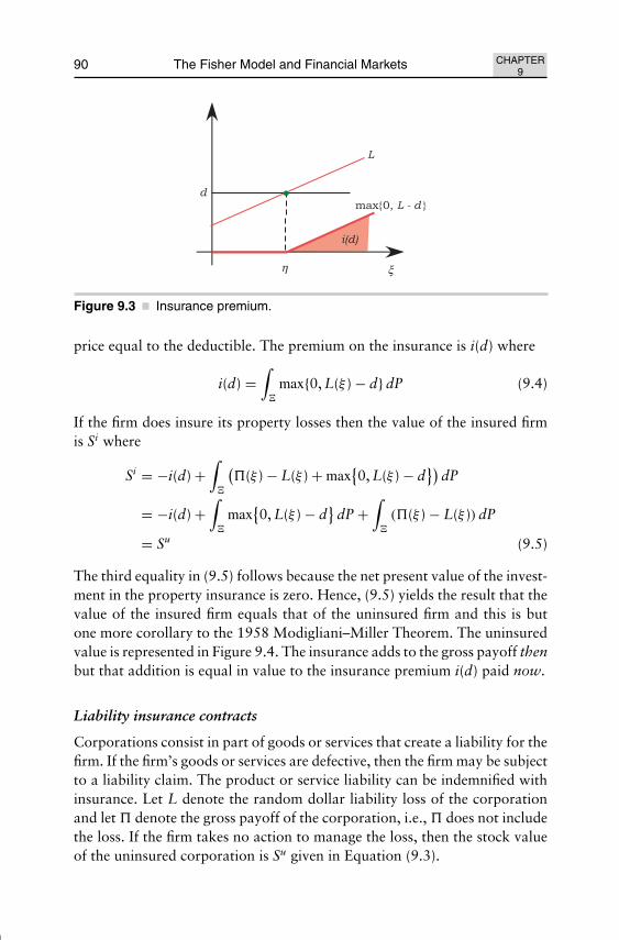
August 18, 2005 11:42 SPI-B312 The Fisher Model and Financial Markets (ED: Chean Chian) ch09
90 The Fisher Model and Financial Markets CHAPTER9
Figure 9.3 Insurance premium.
price equal to the deductible. The premium on the insurance is i(d) where
i(d) =∫
�
max{0, L(ξ ) − d} dP (9.4)
If the firm does insure its property losses then the value of the insured firmis Si where
Si = −i(d) +∫
�
(�(ξ ) − L(ξ ) + max
{0, L(ξ ) − d
})dP
= −i(d) +∫
�
max{0, L(ξ ) − d
}dP +
∫�
(�(ξ ) − L(ξ )) dP
= Su (9.5)
The third equality in (9.5) follows because the net present value of the invest-ment in the property insurance is zero. Hence, (9.5) yields the result that thevalue of the insured firm equals that of the uninsured firm and this is butone more corollary to the 1958 Modigliani–Miller Theorem. The uninsuredvalue is represented in Figure 9.4. The insurance adds to the gross payoff thenbut that addition is equal in value to the insurance premium i(d) paid now.
Liability insurance contracts
Corporations consist in part of goods or services that create a liability for thefirm. If the firm’s goods or services are defective, then the firm may be subjectto a liability claim. The product or service liability can be indemnified withinsurance. Let L denote the random dollar liability loss of the corporationand let � denote the gross payoff of the corporation, i.e., � does not includethe loss. If the firm takes no action to manage the loss, then the stock valueof the uninsured corporation is Su given in Equation (9.3).

August 18, 2005 11:42 SPI-B312 The Fisher Model and Financial Markets (ED: Chean Chian) ch09
CHAPTER9
Corporate Risk Management 91
Figure 9.4 Insured and uninsured values with property insurance.
Liability insurance contracts often indemnify the corporation againstlosses up to some upper limit k. Then the insurance contract payoff ismin{L, k} and the insurance premium is i(k) where
i(k) =∫
�
min{L, k
}dP (9.6)
If the firm does insure its property losses, then the value of the insured firmis Si where
Si = −i(k) +∫
�
(�(ξ ) − L(ξ ) + min
{L(ξ ), k
})dP
= −i(k) +∫
�
min{L(ξ ), k
}dP +
∫�
(�(ξ ) − L(ξ )) dP (9.7)
= Su
The third equality again follows because the net present value of the invest-ment in insurance is zero. The gross value is shown in Figure 9.5. The addi-tional payoff created then just equals the premium paid now on the liabilitypolicy. Hence, (9.7) yields the result that the value of the insured firm equalsthat of the uninsured firm and this is but one more corollary to the 1958Modigliani–Miller Theorem.
Risk Management and Value
Risk management is all about the creation or preservation of value. Incen-tives can be realigned by restructuring the nexus of risks we call the firm. In

August 18, 2005 11:42 SPI-B312 The Fisher Model and Financial Markets (ED: Chean Chian) ch09
92 The Fisher Model and Financial Markets CHAPTER9
Figure 9.5 Insured and uninsured values with liability insurance.
some cases the incentives become misaligned due to hidden actions. Thoseincentives can be realigned by bundling contracts to provide credible assur-ances that the appropriate actions will be taken. In other cases the incentivesbecome misaligned due to hidden knowledge. Even if credible informationthat reveals what is hidden cannot be given to the market participants, it isstill sometimes possible to manage the risks so that optimal decisions thatmaximize value are still feasible. Equivalently, the agency costs due to hiddenknowledge can be avoided if the risks are managed appropriately.
Hidden action
The hidden action problem exists when actions can be taken by manage-ment that affect the value of the stakeholders interests in the firm. The hid-den action problem can be the source of a variety of problems, includingthe risk shifting problem and the under-investment problem. Mayers andSmith (1987) described an under-investment problem in the context of aninsurance market. There the firm made an investment in capital goods thatwere subsequently subject to a possible loss in value and the consequent lossin productive capability. The action that was hidden was the firm’s choiceto take the action to reconstitute the capital goods subsequent to a loss sothat the productive capability was maintained. The problem generated anagency cost for the debt issue used to finance the investment. The problemwas solved by including a bond covenant requiring sufficient insurance. Thebond covenant provided credible assurance that the capital goods would bereconstituted and so the covenant eliminated the agency cost, i.e., see Garvenand MacMinn (1993).
August 18, 2005 11:42 SPI-B312 The Fisher Model and Financial Markets (ED: Chean Chian) ch09
CHAPTER9
Corporate Risk Management 93
Jensen and Meckling described a risk shifting problem. In the classicversion of the problem, corporate management finances a capital investmentproject with a bond issue. The management may choose one of two mutuallyexclusive investment projects. Both projects require the same capital expen-diture but one is riskier than the other in the Rothschild–Stiglitz sense.4 Theability of management to shift risk to bondholders by switching from a lowrisk to a high risk investment project creates the problem, e.g., see Jensenand Meckling (1976), Green (1984) and MacMinn (1993).5 The risk shift-ing problem has been solved in a variety of ways, e.g., see MacMinn (1987).The ability that management has to shift risk creates the problem and so itcan be solved by providing bondholders with a credible assurance that man-agement will not shift the risk. If bonds are issued with a conversion optionthat yields an option value at least as great as the potential devaluation fromrisk shifting, then that is a credible assurance and is one way to solve thisagency problem.
Hidden knowledge
The hidden knowledge problem occurs when some market agents possessinformation that is not available to others. From a corporate perspective ityields a necessary distinction between insiders and outsides, or equivalentlybetween those who do and those who do not have the information. For thisto be meaningful, of course, the information must by its nature have somevalue. In this setting as in Chapter 8, it is supposed that the insiders haveknowledge about the characteristics of the corporate cash flow; the insiderssimply know which of two possible cash flows the corporation has from aninvestment project. The information has value because it yields the correctnet present value for the project.
4This is the notion that one random project payoff can be described as a mean preserving spreadof the other project payoff or equivalently that it has more weight in the tails of its distribution.See Rothschild, M. and J. E. Stiglitz (1970). “Increasing Risk: I. A Definition.” Journal ofEconomic Theory 2: 225–243. Also see MacMinn, R. (1981). Lecture Notes on Rothschild andStiglitz. “Increasing Risk: I. A Definition” at http://macminn.org/uncertainty/risk/rothschild-stiglitz.pdf5There are other examples. The firm must make operating decisions and those decisions are madesubsequent to the investment and so the financing decisions. The production decisions are hiddenand so a potential source of problems. If the corporate payoff is �(q, ξ ) and � satisfies the prin-ciple of increasing uncertainty, i.e., see Leland, H. (1972). “Theory of the Firm Facing UncertainDemand.” American Economic Review 62: 278–291, MacMinn, R. D. and A. Holtmann (1983).“Technological Uncertainty and the Theory of the Firm.” Southern Economic Journal 50:120–136, then it follows that increasing the production increases risk. It is a simple matterto show that the levered firm has an incentive to produce more than the unlevered firm if thedebt is risky.

August 18, 2005 11:42 SPI-B312 The Fisher Model and Financial Markets (ED: Chean Chian) ch09
94 The Fisher Model and Financial Markets CHAPTER9
Figure 9.6 Cash flow time line.
Consider a slightly expanded version of the Fisher model here to motivaterisk management in the presence of the hidden knowledge problem. Previ-ously, we showed that the corporate manager would make decisions to max-imize current shareholder value minus an agency cost; recall that safe debtwill be used if possible because it can eliminate the agency cost and allow theoptimal investment. Froot et al. (1993) noted “. . . if capital market imperfec-tions make externally obtained funds more expensive than those generatedinternally, they can generate a rationale for risk management.” If the firm hasan uncertain cash flow to use in financing its investment and does not man-age that risk, then it must either raise cash from external sources if necessaryor alter the level of its investment. Either response is simply a reaction tothe agency cost. The choice is not actually so stark. The corporate objectivefunction that has been developed shows that the investment will be pushedto the point at which the marginal value of the last dollar invested equalsa dollar plus the marginal agency cost. Hence, the firm will raise cash fromexternal sources but the amount will be limited due to the agency cost. Themodel developed here is motivated by the Froot et al. model but the objectivefunction and agency cost are endogenous just as in previous chapters.
Suppose the timeline is extended so that we have dates t = 0, 1, and 2and refer to those dates as now, then and later, respectively. The firm hasmade decisions in the past, i.e., before now, and those decisions have gen-erated an uncertain payoff then of �1 dollars. In addition, the firm maymake an investment decision then that yields a payoff of �2(I1, ξ2; g) later,if the firm has a good quality investment project and �2(I1, ξ2; b) otherwisewhere �2(I1, ξ2; g) > �2(I1, ξ2; b) for all ξ2. The cash flows are summarizedin Figure 9.7. The investment then is financed with retained earnings, debtor equity. The hidden knowledge problem will apply to the investment pay-off later but not the payoff �1 then from previous corporate decisions. Thehidden knowledge makes retained earnings, or safe debt preferable to thealternatives. If retained earnings and the safe debt capacity do not suffice,then the risks must be actively managed to allow the firm to avoid the agencycost associated with the hidden knowledge.

August 18, 2005 11:42 SPI-B312 The Fisher Model and Financial Markets (ED: Chean Chian) ch09
CHAPTER9
Corporate Risk Management 95
Consider the value of the firm now. Let �t denote the set of states ofnature then and later, i.e., for t = 1 and 2 respectively. Similarly, let pt(ξt) bethe price of a basis stock that pays one dollar in state ξt and zero otherwiseand let Pt(ξt) be the sum of the basis stock prices from zero to ξt. Let St
denote the stock value of the firm at t = 0, 1, 2. Then the stock value now ofthe unhedged firm with the good investment opportunity is Su
0(I1; g) where
Su0(I1; g) =
∫�1
�u1(ξ1) dP1 +
∫�2
�2(I1, ξ2; g) dP2 (9.8)
Of course, the corporate manager does not make the investment decisionnow. Rather she makes that decision then when the cash flow �1(ξ1) fromthe corporate operations is known. Assuming that the cash flow is retained,the stock value then is Su
1(I1; g) where
Su1(I1; g) = �u
1(ξ1) +∫
�2
�2(I1, ξ2; g) dP2 (9.9)
The manager of this unhedged corporation with the good investment projectmakes the investment decision to maximize Su
1(I1; g) − I1 − ca(I1) where ca
is the agency cost.6 Let I∗1 maximize Su
1(I1; g) − I1 so that it is the investmentthat maximizes the net present value or equivalently the current shareholdervalue. This I∗
1 is first best investment but will only be selected if the agencycost is zero. The manager making this investment decision then knows thecorporate earnings �u
1(ξ1) and the manager knows how much safe debt canbe issued in the presence of the hidden knowledge problem. Given rationaleexpectations about the size of the investments made by firms with good andbad projects, the maximum promised payment that the manager can makeand avoid any agency cost due to the hidden knowledge is the dollar promiseb∗
2 = �2(I1, 0; b)7 as shown in Figure 9.7. Let D1(b∗2) be the value of the debt
issue where
D1(b∗2) =
∫�2
b∗2 dP2 (9.10)
Now it is apparent that the manager of the firm with the good investmentproject can avoid the agency cost of the hidden knowledge problem if thecorporate earnings now and the safe debt capacity suffice to raise the optimalinvestment expenditure. Equivalently, the agency cost can be eliminated if�u
1(ξ1) + D1(b∗
2) > I∗1. Without further action, there is no guarantee that this
inequality will be satisfied then.
6See Chapter 8 for the derivation of this objective function.7Of course, if �2(I1, 0; b) = 0 then there is no feasible safe debt issue.

August 18, 2005 11:42 SPI-B312 The Fisher Model and Financial Markets (ED: Chean Chian) ch09
96 The Fisher Model and Financial Markets CHAPTER9
Figure 9.7 Safe debt capacity given hidden knowledge.
ξ1
Figure 9.8 Hedging to manage the risk of earnings then.
Consider the manager making decisions now. The manager is not dueto make a decision about the size of the investment in the capital projectuntil then, but the manager can make decisions now to manage the risk of hav-ing enough money then to make the optimal investment choice. Without anyrisk management decisions now, the firm may or may not have enough cashflow then from corporate operations to finance the optimal investment withretained earnings and safe debt. Hence, in the absence of risk management,the firm may have to raise additional money externally with a risky bondissue or an equity issue. In either case, the associated agency cost will causean under-investment problem and value will be lost. With risk management

August 18, 2005 11:42 SPI-B312 The Fisher Model and Financial Markets (ED: Chean Chian) ch09
CHAPTER9
Corporate Risk Management 97
decisions now, it is possible to eliminate or at least alleviate the agency costsdue to the hidden knowledge problem.
Consider risk management decisions that can be made now that will cir-cumvent the under-investment problem. Suppose the manager hedges thecorporate earnings then by purchasing a forward contract. Also suppose thatsafe debt can be issued on the investment project undertaken then and let b∗
2 bethe maximum promised payment consistent with a transparent valuation ofthe debt issue by outsiders. The forward contract will yield a corporate payoffthen of�h
1(ξ1) = �u1(ξ1)+ϕ(f1 − �(ξ1)) and the debt issue will yield a cash flow
then of D1(b∗2). If the hedge can be designed so that �h
1(ξ1) ≥ I∗1 − D1(b∗
2) forall ξ1, then these risk management and financing decisions combine to elimi-nate the under-investment problem. If the corporate payoff then is increasingacross states, then the under-investment problem can be eliminated by creat-ing a hedge sufficient to make �h
1(0) ≥ I∗1 − D1(b∗
2), i.e., see Figure 9.8.
Sh0(I∗
1; g) =∫
�1
�h1(ξ1) dP1 +
∫�2
�2(I∗1, ξ2; g) dP2
=∫
�1
�u1(ξ1) dP1 + ϕ
∫�1
(f1 − �(ξ1)
)dP1 +
∫�2
�2(I∗1, ξ2; g) dP2
=∫
�1
�u1(ξ1) dP1 +
∫�2
�2(I∗1, ξ2; g) dP2 (9.11)
=∫
�1
�u1(ξ1) dP1 +
∫�2
�2(Ia1, ξ2; g) dP2
+(∫
�2
�2(I∗1, ξ2; g) dP2 −
∫�2
�2(Ia1, ξ2; g) dP2
)= Su
0(Ia1; g) + ca(Ia
1)
The second equality in (9.11) follows because the net present value of theforward position is zero. This is due to the corollary of the 1958 Modigliani–Miller Theorem and becomes quite useful here because the cost of hedging iszero but unlike the corollary, there is value to be gained here by managing therisk of having enough retained earnings available for investment then. Hence,the firm can increase value through appropriate risk management decisionsdesigned to eliminate the agency cost associated with the hidden knowledgeproblem. Equation (9.11) shows that risk management can recapture theentire agency cost.
Caviar Caveat
Hedging can sometimes increase risk and so risk management notions mustbe used carefully and in some cases avoided because they increase rather
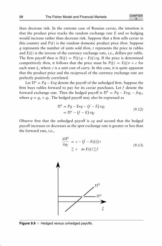
August 18, 2005 11:42 SPI-B312 The Fisher Model and Financial Markets (ED: Chean Chian) ch09
98 The Fisher Model and Financial Markets CHAPTER9
than decrease risk. In the extreme case of Russian caviar, the intuition isthat the product price tracks the random exchange rate E and so hedgingwould increase rather than decrease risk. Suppose that a firm sells caviar inthis country and P(ξ ) is the random domestic product price then. Supposeq represents the number of units sold then, r represents the price in rublesand E(ξ ) is the inverse of the currency exchange rate, i.e., dollars per ruble.The firm payoff then is �(ξ ) = P(ξ ) q − E(ξ ) rq. If the price is determinedcompetitively then, it follows that the price must be P(ξ ) = E(ξ )r + c foreach state ξ , where c is a unit cost of carry. In this case, it is quite apparentthat the product price and the reciprocal of the currency exchange rate areperfectly positively correlated.
Let �u = Pq − Erq denote the payoff of the unhedged firm. Suppose thefirm buys rubles forward to pay for its caviar purchases. Let f denote theforward exchange rate. Then the hedged payoff is �h = Pq − Erqs − frqf ,where q = qs + qf . The hedged payoff may also be expressed as
�h = Pq − Erq − (f − E
)rqf
= �u − (f − E
)rqf
(9.12)
Observe first that the unhedged payoff is cq and second that the hedgedpayoff increases or decreases as the spot exchange rate is greater or less thanthe forward rate, i.e.,
∂�h
∂qf= c − (
f − E(ξ ))
r
>< c as E(ξ )>< f
(9.13)
Figure 9.9 Hedged versus unhedged payoffs.

August 18, 2005 11:42 SPI-B312 The Fisher Model and Financial Markets (ED: Chean Chian) ch09
CHAPTER9
Corporate Risk Management 99
and so the hedged payoff rotates counter clockwise through the forward rateas the hedge increases. This, however, increases rather than decreases the riskof the payoff and provides one strikingly simple example of when a hedge isreally speculation.
Suggested Problems
1. A generalization of 1958 Modigliani–Miller Theorem suggests that iffirms r and t merge so that the payoff of the merged firm is the sumof the payoffs of the unmerged firms, then the stock value of the mergedfirm equals the sum of the values of the unmerged firms. Demonstrate thisclaim.
2. Suppose the corporation described in the section on hidden knowledgefaces random liability losses of L dollars then. Will an insurance purchasebe an effective management technique in solving the under-investmentproblem described there?
3. Consider the corporation described in the section on hidden knowledge.Suppose the corporation has random earnings then from its operationsin the domestic and foreign markets and has investment opportunitiesin both markets then as well. Should the firm hedge the currency risksnow? What other risk management techniques might increase corporatevalue? If the firm levers its capital investments, then where should it dothe borrowing?

August 18, 2005 11:42 SPI-B312 The Fisher Model and Financial Markets (ED: Chean Chian) ch10
Chapter 10Concluding Remarks
T he Fisher model provides the foundation for more than a demonstrationof the origins of the net present value rule under certainty. The received
theory of corporate finance can be posited in the context of the Fisher modelunder uncertainty as the analysis here has shown. The separation theoremsin Chapters 4 and 8 are particularly important because they provide thebasis for an endogenous determination of the corporate objective function.The objective function does not need to be and in fact should not be assumedas it so often has been in the literature.
The modeling also provides a framework for stating and proving theclassic theorems in corporate finance some of which were demonstrated inChapter 6. In the subsequent chapters the hidden action and hidden know-ledge problems were exposited. The hidden action problem arises when cor-porate management can make decisions and take actions that affect the valueof corporate assets unknown to the stakeholders who value those assets inthe financial markets. The hidden action problem is the source of a varietyof agency problems in corporate finance. The risk shift problem arises due toa hidden action and can be solved by reconstructing the risks that constitutethe corporation as was demonstrated in Chapter 7. The under-investmentproblem can arise in a variety of ways and the hidden action problem is onecause of the problem as was demonstrated in Chapter 7 also. The hiddenknowledge problem arises when corporate management possesses informa-tion that investors do not. This information is valuable but difficult at best toconvey to investors or equivalently corporate outsiders. Hidden knowledgeis also the source of agency problems in corporate finance and the most well-known consequence of hidden knowledge is an under-investment problem.
100
August 18, 2005 11:42 SPI-B312 The Fisher Model and Financial Markets (ED: Chean Chian) ch10
CHAPTER10
Concluding Remarks 101
Even though the hidden knowledge problem complicates the analysis becausecorporate insiders cannot trade on the basis of insider information, a sepa-ration result was still demonstrated in Chapter 8 in the process of demon-strating the Myers–Majluf pecking order theorem.
The Fisher model also provides a natural place to begin a study ofcorporate risk management. Most of the theorems in corporate finance areconcerned with capital structure or dividend policy but these concepts areconcerned with packaging or repackaging risks and can be viewed as specialcases of risk management. Some risk management notions are introducedin Chapter 9. The risk shifting problem and an under-investment problemboth due to hidden actions are reconsidered in Chapter 9; risk managementsolutions to these problems exist and are discussed. The hidden knowledgeproblem and the consequent under-investment problem is also discussed anda risk management solution provided by Froot et al. is reframed and demon-strated in the Fisher setting.
The Fisher model provides the framework and basis for generating allof the important theorems in corporate finance. Some of the classic theo-rems have been demonstrated here but far more is possible. The model issufficiently malleable for generalizations and theorems not yet stated.

August 18, 2005 11:40 SPI-B312 The Fisher Model and Financial Markets (ED: Chean Chian) bib
This page intentionally left blankThis page intentionally left blank

August 18, 2005 11:40 SPI-B312 The Fisher Model and Financial Markets (ED: Chean Chian) bib
Bibliography
Alchian, A. A. and H. Demsetz (1972). “Production, Information Costs, and Eco-nomic Organization.” American Economic Review 62(5): 777–795.
Allen, F. and G. R. Faulhaber (1989). “Signaling by Underpricing in the IPO Market.”Journal of Financial Economics 23(2): 303–323.
Arrow, K. J. (1963). “The Role of Securities in the Optimal Allocation of Risk Bear-ing.” Review of Economic Studies 31(2): 91–96.
Arrow, K. J. (1984). “The Theory of Risk Aversion.” Collected Papers of Kenneth J.Arrow 3: 147–171. Harvard University Press.
Baron, D. P. (1976). “Default Risk and the Modigliani–Miller Theorem: A Synthesis.”American Economic Review 66(1): 204–212.
Bhattacharya, S. (1980). “Nondissipative Signaling Structures and Dividend Policy.”Quarterly Journal of Economics 95(1): 1–24.
Bodie, Z. and R. Taggart (1978). “Future Investment Opportunities and the Valueof the Call Provision on a Bond.” Journal of Finance 33: 1187–1200.
Brennan, M. and A. Kraus (1987). “Efficient Financing under Asymmetric Informa-tion.” Journal of Finance XLII(5): 1225–1243.
DeAngelo, H. and R. Masulis (1980). “Optimal Capital Structure Under Corporateand Personal Taxation.” Journal of Financial Economics 8: 3–29.
Debreu, G. (1959). Theory of Value: An Axiomatic Analysis of Economic Equilib-rium. John Wiley & Sons.
Diamond, P. (1967). “The Role of a Stock Market in a General Equilibrium Modelwith Technological Uncertainty.” American Economic Review 57: 759–773.
Ekern, S. and R. Wilson (1974). “On the Theory of the Firm in an Economy withIncomplete Markets.” Bell Journal of Economics 5: 171–180.
Feder, G. et al. (1980). “Futures Market and the Theory of the Firm Under PriceUncertainty.” Quarterly Journal of Economics XCIV: 317–328.
Fisher, I. (1930). The Theory of Interest. New York, MacMillan.
103
August 18, 2005 11:40 SPI-B312 The Fisher Model and Financial Markets (ED: Chean Chian) bib
104 The Fisher Model and Financial Markets BIBLIOGRAPHY
Froot, K. A. et al. (1993). “Risk Management: Coordinating Corporate Investmentand Financing Policies.” Journal of Finance 48(5): 1629–1658.
Froot, K. A. et al. (1994). “A Framework for Risk Management.” Harvard BusinessReview Nov–Dec: 91–102.
Garman, M. (1979). A Synthesis of the Pure Theory of Arbitrage. Working PaperNo. 98, Institute of Business and Economic Research, University of Californiaat Berkeley.
Garven, J. R. and R. D. MacMinn (1993). “The Underinvestment Problem, BondCovenants and Insurance.” Journal of Risk and Insurance 60(4): 635–646.
Glazer, J. and R. Israel (1990). “Managerial Incentives and Financial Signaling inProduct Market Competition.” International Journal of Industrial Organiza-tion 8(2): 271–280.
Green, R. C. (1984). “Investment Incentives, Debt and Warrants.” Journal of Finan-cial Economics 13: 115–136.
Hirshleifer, J. (1965). “Investment Decision Under Uncertainty: Choice-TheoreticApproaches.” Quarterly Journal of Economics 79(4): 509–536.
Holthausen, D. (1979). “Hedging and the Competitive Firm Under Price Uncer-tainty.” American Economic Review 69: 989–995.
Jensen, M. and W. Meckling (1976). “Theory of the Firm: Managerial Behavior,Agency Costs and Ownership Structure.” Journal of Financial Economics 3:305–360.
Jensen, M. and C. Smith (1985). “Stockholder, Manager, and Creditor Interests:Applications of Agency Theory.” Recent Advances in Corporate Finance.E. Altman and M. Subrahmanyam, eds. Richard D. Irwin.
Kimball, M. S. (1990). “Precautionary Saving in the Small and in the Large.” Econo-metrica 58: 53–73.
Kohn, M. (1999). Risk Instruments in the Medieval and Early Modern Economy.Working Paper 99-07, Dartmouth College.
Leland, H. (1972). “Theory of the Firm Facing Uncertain Demand.” American Eco-nomic Review 62: 278–291.
Leland, H. and D. Pyle (1977). “Informational Asymmetries, Financial Structure andFinancial Intermediation.” Journal of Finance 32: 371–387.
MacMinn, R. (1980). Lecture Notes on Arrow’s “The Theory of Risk Aversion”.MacMinn, R. (1981). Lecture Notes on Rothschild and Stiglitz’s “Increasing Risk: I.
A Definition”.MacMinn, R. (1984). Lecture Notes on Pratt’s “Risk Aversion in the Small and in
the Large”.MacMinn, R. (1987). “Lecture Notes on the Risk-Shifting Problem.”MacMinn, R. (1995). Lecture Notes on Ekern and Wilson’s “On the Theory of the
Firm in an Economy with Incomplete Markets”.MacMinn, R. D. (1987). “Forward Markets, Stock Markets, and the Theory of the
Firm.” Journal of Finance 42(5): 1167–1185.MacMinn, R. D. (1987). “Insurance and Corporate Risk Management.” Journal of
Risk and Insurance 54(4): 658–677.MacMinn, R. D. (1993). “On the Risk Shifting Problem and Convertible Bonds.”
Advances in Quantitative Analysis of Finance and Accounting 2: 181–200.
August 18, 2005 11:40 SPI-B312 The Fisher Model and Financial Markets (ED: Chean Chian) bib
BIBLIOGRAPHY The Fisher Model and Financial Markets 105
MacMinn, R. D. and A. Holtmann (1983). “Technological Uncertainty and the The-ory of the Firm.” Southern Economic Journal 50: 120–136.
MacMinn, R. and J. Martin (1988). “Uncertainty, the Fisher Model, and Corpo-rate Financial Theory.” Research in Finance 7. Greenwich, Connecticut, JAIPress Inc.
MacMinn, R. and F. Page (1995). “Stock Options, Managerial Incentives, and CapitalStructure.” Journal of Financial Studies Dec.
Main, B. G. (1983). “Corporate Insurance Purchases and Taxes.” Journal of Riskand Insurance 197–223.
Markowitz, H. M. (1952). “Portfolio Selection.” Journal of Finance 7(1): 77–91.Mayers, D. and C. Smith (1982). “On the Corporate Demand for Insurance.” Journal
of Business 55: 281–296.Mayers, D. and C. W. J. Smith (1987). “Corporate Insurance and the Underinvest-
ment Problem.” Journal of Risk and Insurance 45–54.McNichols, M. and A. Dravid (1990). “Stock Dividends, Stock Splits, and Signaling.”
Journal of Finance 45(3): 857–879.Miller, M. and F. Modigliani (1961). “Dividend Policy, Growth, and the Valuation
of Shares.” Journal of Business 34(4): 411–433.Miller, M. H. (1977). “Debt and Taxes.” Journal of Finance 32(2): 261–275.Modigliani, F. and M. H. Miller (1958). “The Cost of Capital, Corporation
Finance and the Theory of Investment.” American Economic Review 48(2):261–297.
Mossin, J. (1966). “Equilibrium in a Capital Asset Market.” Econometrica 34:768–783.
Myers, S. C. (1977). “The Determinants of Corporate Borrowing.” Journal of Finan-cial Economics 5: 147–175.
Myers, S. C. and N. S. Majluf (1984). “Corporate Financing and Investment Deci-sions When Firms Have Information That Investors Do Not Have.” Journal ofFinancial Economics 13: 187–221.
Noe, T. (1988). “Capital Structure and Signaling Game Equilibria.” Review of Finan-cial Studies 1: 331–356.
Pratt, J. W. (1964). “Risk Aversion in the Small and in the Large.” Econometrica 32:122–136.
Radner, R. (1974). “A Note on Unanimity of Stockholder’s Preferences Among Alter-native Production Plans: A Reformulation of the Ekern-Wilson Model.” BellJournal of Economics 5: 181–184.
Riley, J. G. (1985). “Competition with Hidden Knowledge.” Journal of PoliticalEconomy 93(5): 958–976.
Rothschild, M. and J. E. Stiglitz (1970). “Increasing Risk: I. A Definition.” Journalof Economic Theory 2: 225–243.
Sandmo, A. (1970). “The Effect of Uncertainty on Saving Decisions.” Review ofEconomic Studies 37: 353–360.
Sharpe, W. F. (1964). “Capital Asset Prices: A Theory of Market Equilibrium UnderConditions of Risk.” Journal of Finance 19(3): 425–442.
Smith, C. and J. Warner (1979). “On Financial Contracting: An Analysis of BondCovenants.” Journal of Financial Economics 7: 117–161.

August 18, 2005 11:40 SPI-B312 The Fisher Model and Financial Markets (ED: Chean Chian) bib
106 The Fisher Model and Financial Markets BIBLIOGRAPHY
Smith, C. W. and R. M. Stulz (1985). “The Determinants of Firms’ Hedging Policies.”Journal of Financial and Quantitative Analysis 20(4): 391–405.
Sobel, J. et al. (1990). “Fixed-Equilibrium Rationalizability in Signaling Games.”Journal of Economic Theory 52(2): 304–331.
Stiglitz, J. E. (1969). “A Re-Examination of the Modigliani–Miller Theorem.”American Economic Review 59(5): 78–93.
Stulz, R. M. (1984). “Optimal Hedging Policies.” Journal of Financial and Quanti-tative Analysis 19(2): 127–140.

August 18, 2005 11:42 SPI-B312 The Fisher Model and Financial Markets (ED: Chean Chian) index
Index
agency cost, 55, 58–60, 62, 70–73, 78,79, 82, 83, 85, 86, 92, 94–97
agency problems, xi, 53–55, 58, 62, 63,85, 93, 100
asset substitution, 52, 53, 85asymmetric information, 53, 67, 68, 82
basis asset, 13, 16, 68, 73basis stock, x, 16–22, 29, 50, 57, 95bond covenant, 54, 55, 64, 86, 92budget constraint, 2, 3, 7, 9, 12–14,
27, 31–33, 75
call option, 25, 26, 37–39, 41, 42, 60,89
capital structure, xi, 22, 40, 44–47, 49,52, 68, 71, 74, 82, 87, 101
complete market, 13, 30, 52conflict of interest, 44, 54, 58consumption pair, 2–4, 13, 15, 20, 27credible commitment, 85
1980 DeAngelo–Masulis Theorem, 52debt, xi, 22–25, 33, 35–40, 42, 44–56,
58, 60–62, 64, 65, 67, 71, 72, 79,80, 82, 83, 85, 86, 92–95, 97
debt over-hang, 65, 66, 85, 86deductible, 43, 49, 50, 89, 90
dilution, 70, 77, 83, 86dividends, 44, 47–49, 68, 101
equity, xi, 22, 25, 31, 37, 38, 40, 41,44–50, 55, 58, 60, 62, 67, 70,72–75, 77, 82, 83, 86, 94, 96
expected utility, x, 2, 13, 15, 16, 20,55, 75
Fisher separation, x, 8, 9, 11, 27–30,32, 33, 35, 77, 81
futures contract, 47, 88
hedged, 47, 70, 71, 88, 89, 98, 99hidden action, xi, 53, 67, 73, 85–87,
92, 100, 101hidden knowledge, xi, 67–75, 77, 82,
85–87, 92–97, 99–101
indemnified, 90indifference curves, 3, 4, 10, 20internal rate of return, 6, 7, 10, 11investment frontier, 2, 5, 7, 8, 10, 11,
34investment project, x
levered, 26, 35, 37–40, 44, 45, 49–53,57, 58, 63, 71, 72, 82, 93
liability insurance, 90–92
107

August 18, 2005 11:42 SPI-B312 The Fisher Model and Financial Markets (ED: Chean Chian) index
108 The Fisher Model and Financial Markets INDEX
marginal efficiency of investment, 5, 6,8, 10
marginal rate of substitution, 3–5,14–16, 19
1958 Modigliani–Miller Theorem, xi,40, 44–46, 49, 59, 62, 84, 86, 87,89–91, 97, 99
1961 Miller–Modigliani Theorem, 47,49
1963 Modigliani–Miller Theorem, 491977 Miller Theorem, 52
net future value, 6net present value, ix, x, 1, 2, 6, 9, 10,
27, 28, 30, 32, 35, 36, 44, 52, 54,64, 73, 86, 89–91, 93, 95, 97, 100
nexus of contracts, xi, 47, 84, 86
option, x, 22, 25, 26, 28, 32–39, 41,60, 61, 74, 83, 93
pecking order, xi, 52, 67, 82, 83, 101premium, 43, 87, 90, 91
probability, 13, 14, 17–19, 29, 33, 63,64, 66, 69, 74, 77, 83, 85
property insurance, 89–91proprietor, x, 2, 6–11, 28–30, 35
risk aversion, 16, 17, 19–21, 29, 32,54, 55, 73, 74, 77
risk-shifting, xi, 52–55, 57, 62, 66, 67,85–87, 92, 93, 101
risky debt, 24, 46, 83
safe debt, 24, 34, 39, 46, 73, 82, 83,94–97
share price, 22–24, 35
tax shield, 49, 52time value of money, 1
under-investment, xi, 53, 63, 64, 66,67, 79, 82, 85–87, 92, 96, 97,99–101
weighted cost of capital, 26, 46