Federal Reserve Bank of Minneapolis

Dimensions of Inequality: Facts on the U.S. Distributions of Earnings, Income, and Wealth (p. 3) Javier Dfaz-Gimenez Vincenzo Quadrini Jos6-Victor Rfos-Rull

Understanding the U.S. Distribution of Wealth (p. 22) Vincenzo Quadrini Jose-Victor Rfos-Rull

Federal Reserve Bank of Minneapolis

Quarterly Review ISSN 0271-5287

Vol. 21, No. 2

This publication primarily presents economic research aimed at improving policymaking by the Federal Reserve System and other governmental authorities.

Any views expressed herein are those of the authors and not necessarily those of the Federal Reserve Bank of Minneapolis or the Federal Reserve System.

Editor: Arthur J. Rolnick Associate Editors: Edward J. Green, Preston J. Miller,

Warren E. Weber Economic Advisory Board: Narayana R. Kocherlakota, Richard Rogerson

Managing Editor: Kathleen S. Rolfe Article Editors: Sarah A. Freier, Kathleen S. Rolfe

Designer: Phil Swenson Associate Designer: Lucinda Gardner

Typesetters: Mary E. Anomalay, Jody Fahland Technical Assistants: Maureen O'Connor, Jason Schmidt Circulation Assistant: Elaine R. Reed

The Quarterly Review is published by the Research Department of the Federal Reserve Bank of Minneapolis. Subscriptions are available free of charge. Quarterly Review articles that are reprints or revisions of papers published elsewhere may not be reprinted without the written permission of the original publisher. All other Quarterly Review articles may be reprinted without charge. If you reprint an article, please fully credit the source—the Minneapolis Federal Reserve Bank as well as the Quarterly Review—and include with the reprint a version of the standard Federal Reserve disclaimer (italicized above). Also, please send one copy of any publication that includes a reprint to the Minneapolis Fed Research Department. A list of past Quarterly Review articles and electronic files of many of them are available through the Minneapolis Fed's home page on the World Wide Web: http://woodrow.mpls.frb.fed.us.

Comments and questions about the Quarterly Review may be sent to Quarterly Review Research Department Federal Reserve Bank of Minneapolis P.O. Box 291 Minneapolis, Minnesota 55480-0291 (612-340-2341 / FAX 612-340-2366). Subscription requests may also be sent to the circulation assistant at err@res.mpls.frb.fed.us; editorial comments and questions, to the managing editor at ksr@res.mpls.frb.fed.us.

Federal Reserve Bank of Minneapolis Quarterly Review Spring 1997

Understanding the U.S. Distribution of Wealth

Vincenzo Quadrini* Jose-Victor Rios-Rulf Assistant Professor Senior Economist Department of Economics Research Department Universitat Pompeu Fabra Federal Reserve Bank of Minneapolis

and Assistant Professor Department of Economics University of Pennsylvania

When U.S. households are ranked according to how much wealth they hold, they form a lopsided picture:1

• The bottom 40 percent of all households have only about 1 percent of all the wealth in the nation.

• The top 1 percent of all households have nearly 30 percent of all the wealth; the top 5 percent, 55 percent of the wealth; and the top 20 percent, 80 percent of the wealth.

• Partly as a result of those two extremes, the standard measure of the dispersion of wealth, the Gini index, is large: 0.78.

Changing these facts about the U.S. wealth distribution has for years been a recurrent theme of political discussions. But before workable policies to change the facts can be formulated, the facts themselves must be understood. Why is the wealth distribution so lopsided? What characteristics in the economy were essential to produce this form of dis-tribution? Providing such an understanding of data is the job of economists, and unfortunately, with regard to the wealth distribution, that job has just begun.

In general, to try to understand facts reflected in data, economists create theories, expressed through mathemati-cal models, that are meant to capture the features that best account for those facts. Then they test the theories by hav-ing the models generate data and comparing the models' data with the facts. In the last few years, economists have

begun to try to develop a theory capable of quantitatively accounting for the U.S. wealth data.

This theory has focused on changes in earnings, the fea-ture economists traditionally have seen as directly affecting different levels of savings and wealth. Households have been thought of as facing temporary shocks to their earn-ings which they cannot insure against in any way other than personal saving. Thus, according to this theory, house-holds must self-insure against random fluctuations in their earnings; households save in good times so that they can dissave in bad times. The wealthy households are those who have experienced streaks of good times in the recent past.

Models incorporating this abstraction have been able to generate a distribution of wealth which replicates some of the properties of the U.S. distribution. However, the resem-

*For contributions to this work, the authors thank Rao Aiyagari, Javier Dfaz-Gimenez, Mark Huggett, and the editors and referees of this journal. Ri'os-Rull thanks the National Science Foundation for financial support. This article is dedicated to the memory of Rao Aiyagari.

'These are 1992 data from the Survey of Consumer Finances. For details on the data and their sources, see the article by Dfaz-Gimenez, Quadrini, and Rfos-Rull else-where in this issue of the Quarterly Review.

The lopsided picture holds if the data are broken down by the age of the head of the household. For households with a head between 35 and 50 years old, the bottom 40 percent of all households have 2.2 percent of total wealth; the top 1 percent, 28 per-cent of total wealth; the top 5 percent, 51 percent; and the top 20 percent, over 75 per-cent; and the Gini index for this age group is 0.76.

22

Vincenzo Quadrini, Jose-Victor Ros-Rull Understanding the U.S. Distribution of Wealth

blance between the models' and the data's distributions is not satisfactory. This suggests that models with only dif-ferent realizations of a common earnings process are miss-ing some features essential to account for the wealth dis-tribution. Other features must be added to the theory of the wealth distribution in order to account for the facts.

Here, we review the progress made so far toward the development of a theory of the wealth distribution. The models that have been used to study the wealth distribution are heterogeneous agent versions of standard neoclassical growth models with uninsurable idiosyncratic shocks to earnings. The equilibria of these models can be found by numerical methods, and the properties of the equilibria can be compared with the properties of the data. These models endogenously generate differences in asset holdings as the result of households' desire to smooth consumption in the presence of time-varying labor earnings. The key feature of these models is, then, that the distribution of earnings is exogenous, while the distribution of wealth is endogenous.

The two dominant types of models used generally in macroeconomics have been used to study the distribution of wealth. The dynastic model includes the infinitely lived agent abstraction and assumes that people care for their descendants as if they were themselves, and the life cycle model includes overlapping generations of finitely lived agents who do not care about their descendants. Thus, the main motive for saving—aside from insuring against shocks to earnings—differs in these two types of models: in dynastic models, people save to improve their descen-dants' consumption, while in life cycle models, people save to improve their own consumption during retirement. Technically, these models are also different in terms of the tools that are used to characterize their equilibrium allo-cations. Moreover, before we can compare the models with the data, the dynastic model requires that we adjust the wealth distribution to eliminate the role of age, while the life cycle model does not. Therefore, the success or failure of one of these types of models is not necessarily related to the success or failure of the other. For all these reasons, these two structures require separate analyses. We demonstrate here that both types of models reproduce the wealth distribution data poorly.

We then review some other features that have been re-cently proposed as worthy complements to the theory of the wealth distribution based on changes in earnings. Some of these extra features are better suited to be embedded in a dynastic model, while others belong in a life cycle mod-el. None of the features has been fully analyzed yet, but

along with the earnings process, they all seem to have the potential to dramatically affect the decisions of households to save.

These extra features tend to apply to people in specific circumstances—primarily, either die rich or the poor, that is, those with either the most or the least wealth. Richer people, for example, are more likely to be entrepreneurs, who have limited ability to borrow in order to finance then-production projects. Richer people are also more likely to be concerned with the higher rates of return that high lev-els of assets can command and with random capital gains. Poorer people, in contrast, are more likely to be affected by government support policies that guarantee minimum con-sumption levels and by changes in health and marital status.

Studies of all these proposed model features represent movements in the right direction. The preliminary findings indicate that including them in models with temporary shocks to earnings will move us closer to being able to un-derstand the U.S. distribution of wealth. The Dynastic Model Again, most of the efforts to understand the wealth dis-tribution have been focused on changes in earnings, and two types of models have been used. Let's look first at the dynastic model. The key property of this type of model is that in it people live forever. The dynastic model thus implicitly assumes a strong linkage of individuals and their progeny. We analyze first the version of this model in which agents' earnings are deterministic. In that ver-sion, the distribution of wealth is indeterminate, which demonstrates the need for a mechanism to generate deter-minate wealth distributions. We analyze then a version of the dynastic model in which agents face idiosyncratic earnings shocks that are not insurable. We call this the stochastic version of the dynastic model even though it has no aggregate uncertainty and it generates determinate wealth distributions. Unfortunately, even though this ver-sion can endogenously generate a distribution of wealth, it cannot adequately reproduce the U.S. wealth distribution data. The Deterministic Version In a dynastic model, households' preferences are generally given by the expected value of a discounted sum of per pe-riod utilities. The model has a production sector that trans-forms capital K and labor N services into output, through an aggregate production function, f(K}N), which in turn can be used either for investment (to increase capital or to make up for the fraction 8 that depreciates) or for con-

23

sumption purposes. In this type of model, households differ in their asset holdings,2 which are denoted by a. To de-scribe the economy at a point in time, we need a descrip-tion of the amount of assets that each agent has. Mathemat-ically the best way to describe the asset amount is through a probability measure over wealth levels, which we denote by x. This measure lets us not keep track of the names of the agents. In this model, all assets are real3 and aggregate capital, the sum of wealth held by all households, is given by the first moment of the measure; that is, K = j a dx. The measure x is a sufficient description of the state of the economy.

The deterministic version of a dynastic model has no shocks that affect households and, hence, no precautionary savings. The market structure assumed is that of a se-quence of markets for capital, labor, and the consumption good. This market structure implements the Pareto optima that are also achieved with an Arrow-Debreu complete market structure. Chatterjee (1994) shows that in this sort of model, the main properties of the distribution of wealth are self-perpetuating and people do not move from one economic level to another. That is, if all households hold the same wealth today, they will all hold the same wealth tomorrow. More precisely, Chatterjee shows that

• With general preferences, the steady state of the econ-omy (a situation in which variables do not change over time) is given by any measure x for which the margin-al productivity of aggregate capital is equal to the rate of time preference.

• With homothetic preferences, if xt(A) is the measure of agents over the subset of asset holdings A at time t, then xt+l(atA) = xt(A\ where at is a positive real number; that is, all agents change their wealth in the same proportion.

Chatterjee (1994) also shows that with more general (but identical across agents) preferences, some of the key fea-tures of the shape of the initial wealth distribution x0 are maintained over time. The deterministic version of the dy-nastic model is, therefore, silent with regard to the wealth distribution because the initial conditions determine cur-rent and future conditions. The Stochastic Version A version of the dynastic model that has stochastic fea-tures at the individual, but not the aggregate, level can be readily constructed in which households are subject to un-insurable idiosyncratic shocks.

Shocks are typically posed as stochastic disturbances on the labor earnings of the households (Aiyagari 1994). One way to put shocks into the model, for example, is to let the efficiency units of each agent, denoted by s e S = { s l v . f o l l o w a Markov chain with transition matrix r[s'\s]. The process for the shocks can accommodate both transitory and permanent components.

To see this, imagine that the economy has / types of agents, types which differ in their long-run average earn-ings. Each type i e {1,...,/} can have 7 possible individual states, some better than others. This framework can be embedded in the general structure by letting T be a block-diagonal matrix, with I blocks denoted by r, of dimension 7x7. In such a model, the probability measure describing the economy x accounts not for the distribution of wealth, but for the joint distribution of shocks and asset holdings. Again, the aggregate capital of the economy is the sum of the assets of all households, K = \ a dx, and aggregate em-ployment is the sum of the efficiency units of labor that each household has and that we normalize to 1; that is, N = jsdx = 1.

In this world, agents save for precautionary reasons to smooth consumption, and the economy can be character-ized as a permanent income world. In good times, agents save a higher proportion of their income than in bad times, and agents with high wealth are those who have had a recent history of good times. The agents' positions in the wealth distribution change over time between a lower bound a (imposed either by the existence of credit con-straints or by the value such that in an agent's worst pos-sible state, the interest payments are not higher than the agent's labor income) and an upper bound a, such that an agent who has assets above this level always (for all s) chooses to have a smaller next-period wealth, since more consumption-smoothing brings no further gains. The exis-tence of this upper bound requires the interest rate to be lower than the rate of time preference; otherwise, agents would not have an upper bound on savings (Huggett 1993, Lemma 1).

A steady state can be defined as a stationary measure x\ a pair of prices for labor and for rental services of cap-ital w and r, a value function for the agents v(s,a), and an

2People might also differ in the wage that they command, since they can have different amounts of efficiency units of labor.

3This does not necessarily mean that agents cannot borrow, since JC can have mass on the negative numbers. It just means that financial capital and real capital are perfect substitutes.

24

Vincenzo Quadrini, Jos-Victor Rfos-Rull Understanding the U.S. Distribution of Wealth

associated decision rule a = g(s,a) such that • The decision rule g solves the problem of the agent:

(1) v{s,a) = maxc>0^[gfl1 u{c) + p£s,lV subject to

(2) c + a - a(\+r) + ws. Equation (1) gives the value to the household that has cur-rent shock 5 and wealth a; this value is equal to the maxi-mum of the utility «(•) that can be obtained from con-sumption c in this period plus the discounted (by P) ex-pected value of having asset holdings a in the next peri-od. Equation (2) is the budget constraint: the sum of cur-rent consumption plus next period's wealth must equal the sum of capital and labor income plus the wealth that was brought into the period. Together, the two equations con-stitute the recursive form of the standard utility maximiza-tion problem subject to a budget constraint.

• The aggregate capital generated by the stationary mea-sure x* induces factor prices r and w defined as

(3) r= f«{Ladx*>1)-5

(4) w = f N ( j s A a d x \ l ) . These are the conditions that factor prices equal marginal productivities.

• The decision rule g(s,a) and the process for the shock T generate the next-period distribution of agents x* ac-cording to this mapping:

(5) *<(S0,A0) = | o for all appropriate sets {50,A0} over which the mea-sure is defined and where X{a'=g(s,a)} m indicator function that takes the value of one if the statement is true and zero otherwise.

This is the steady-state condition: if today's distribution of wealth is jc*, tomorrow's should also be x*. Note that x*(S0,A0) is obtained by counting over all the households (given by the inner integral) that choose to have assets in A0 and have shocks in S0. (The indicator function tells us which households to count, and the transition matrix T tells us how many to count given the previous shock.)

Steady states with a lower interest rate than the rate of time preference have been shown to exist (Laitner 1979 and 1992, Bewley 1984, Clarida 1990, and Aiyagari 1994) and also to be the only type of steady state that can exist (Huggett 1995), although more than one of this type may exist. To achieve this lower interest rate, aggregate capital in the stochastic version of the dynastic model must be higher than aggregate capital in a deterministic version. The difference between these two amounts of capital are referred to as precautionary savings. Steady states can be readily found by iterative procedures. (For a description of the methods involved, see, for example, Aiyagari 1994 or Rios-Rull 1995.)

Note that a key feature of models of this type is that the distribution of earnings is exogenous,4 while the model en-dogenously generates a distribution of income and wealth. Since the interest rate is lower than the rate of time prefer-ence in these models, households save for consumption-smoothing purposes. Hence, the key determinant of sav-ings is not the permanent component of the process for the shock, but rather its transitory component. So the key property of the distribution of earnings in endogenously generating the distribution of wealth is the volatility of in-dividual earnings, not permanent differences in earnings across households (Constantinides and Duffie 1996). In terms of the transition matrices T, what matters is the mo-bility induced by each Tif not the differences across earn-ings types. Empirical Properties In dynastic models with earnings uncertainty, differences in wealth are a function partly of age and partly of the strings of good or bad times in people's lives. People of the same age can, and, in general, will differ in the amount of wealth they hold. Now we can look at what dynastic models imply quantitatively about the wealth distribution, and we can compare these empirical properties with the data.

Examples of dynastic models with precautionary sav-ings to smooth consumption in the presence of uninsur-able earnings uncertainty include those of Aiyagari (1994) and Castaneda, Diaz-Gimenez, and Rios-Rull (1997). These models differ in the process chosen for earnings.

In the baseline parameterization of Aiyagari (1994),

4Slightly more sophisticated versions of these models with an explicit leisure choice would have as exogenous not the distribution of earnings, but the distribution of wages per unit of working time.

25

agents face an uninsurable random stream of yearly labor earnings that follows a first-order autoregressive process in logs with an autocorrelation of 0.6 and a standard de-viation of the innovations of 0.2, which yields an uncondi-tional coefficient of variation of 0.312. These figures are based on estimates from Abowd and Card (1989), who use several panel data. These figures are also consistent with the findings of Heaton and Lucas (1996), who use data from the Panel Study of Income Dynamics. Aiyagari (1994) also considers a process with twice the standard deviation of the innovation for earnings, which results in an unconditional coefficient of variation of 0.625; this is a much higher variability than the estimates in the litera-ture of variations in individual earnings.

Castaneda, Diaz-Gimenez, and Rios-Rull (1997) ex-plore the role that spells of unemployment play in shaping the distribution of income and its cyclical properties. For these researchers, all fluctuations in earnings are associated with changes in employment.5 Castaneda, Diaz-Gimenez, and Rios-Rull study two environments, one in which all agents are ex ante identical and one in which there are five types of ex ante identical agents. Across types, agents dif-fer on their skill level (average wages) and on the process for the spells of unemployment. The process for the spells can be calibrated to observed features of unemployment in the data, such as the level and the duration of unemploy-ment. The version of the model economy with different skill levels shares with the data that unemployment is more likely for agents with lower average wages.6 (For details of the specific calibration, see Rios-Rull 1993 and Castaneda, Diaz-Gimenez, and Rios-Rull 1997.)

Table 1 reports some distributional statistics for U.S. earnings of people 35-50 years old and for the earnings of agents in the four models just discussed. Since these models abstract from life cycle considerations, we try to correct the U.S. data by looking at a subset of ages that excludes both early starters and retirees. The specific age group that we choose does not matter much, as can be seen in the work of Diaz-Gimenez, Quadrini, and Rios-Rull (elsewhere in this issue of the Quarterly Review).

Perhaps the most noticeable feature of Table 1 is that all four models have a lot less earnings inequality than the data do. This is by design. The first three models abstract from any considerations regarding permanent differences in earnings across agents: all differences in the first three models are temporary and are the differences responsible for generating differences in wealth holdings. The last mod-el has differences in average earnings across individuals,

but these differences are from average labor earnings for only five groups. This reduces the importance of the tails of the distribution and so underestimates the variability of earnings. As we will see, in this type of model, what mat-ters in generating wealth dispersion is not permanent dif-ferences in earnings but temporary differences, since the main motive for accumulating wealth is to create a buffer against earnings fluctuations.

Table 1 also reports the same statistics for the distribu-tion of wealth that are reported for earnings. All the model economies generate some wealth concentration, with the first three models generating more wealth concentration than the original earnings concentration, but still a lot less than the wealth concentration found in the U.S. data:

• Regarding the bottom of the distribution, all four mod-els generate a bottom 40 percent of agents who hold considerably more wealth than their counterparts in the data.

• The top groups hold considerably less wealth in the model economies than in the U.S. data, with the same relative performance of the different models. The mod-el that performs best on this measure (Aiyagari's high variability model) accounts for 58 percent of the share of wealth held by the top quintile and 14 percent of the share held by the top 1 percent of the population).

• The Gini indexes are lower in the model economies than in the data.

Overall, we see that Aiyagari's high variability model is the one that performs best, followed by Aiyagari's base-line model and then the unemployment model with iden-tical-skill agents. The unemployment model with differ-ent-skill agents generates the least wealth inequality even though that model has a considerable amount of earnings inequality. This is due to the fact that Aiyagari's two mod-els have more earnings variability at the individual level than the other models do. (The Aiyagari models include all possible sources of individual earnings variability, while the other models include only unemployment fluctuations as sources of earnings variability.) However, even Aiya-

5 Actually, Castaneda, Diaz-Gimenez, and Rios-Rull (1997) study the cyclical fluc-tuations of the distribution of income, so their economy has aggregate fluctuations. From the individual point of view, this feature translates into changes in the process for the employment shock that depends on the aggregate state of the economy. But these changes are small and do not affect the main properties discussed here.

6Krusell and Smith (1996) report basically the same findings in a similar envi-ronment.

26

Vincenzo Quadrini, Jose-Victor Ros-Rull Understanding the U.S. Distribution of Wealth

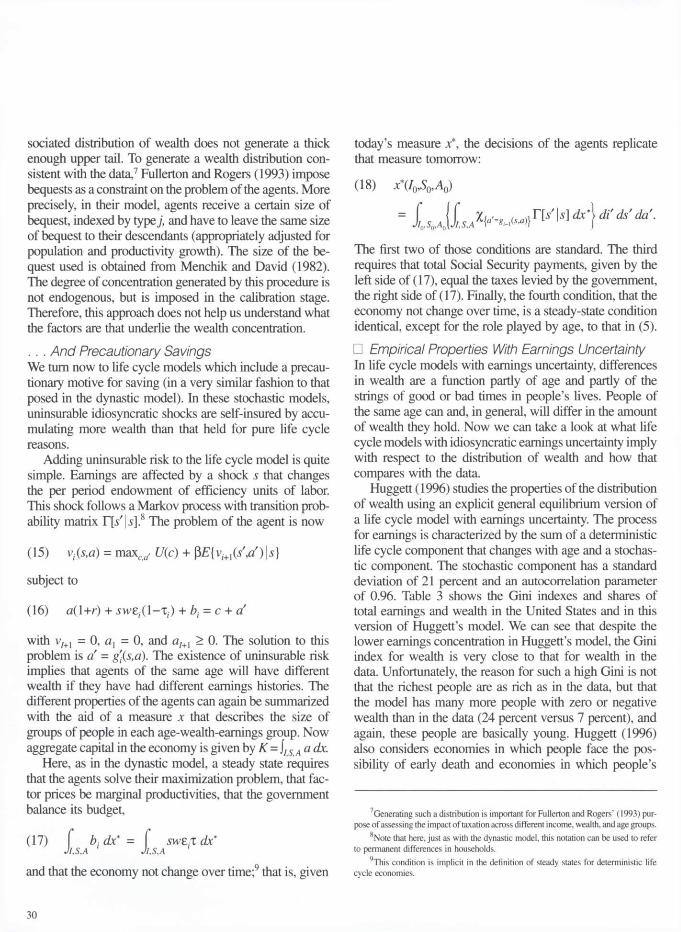
Table 1 Theory Faces Facts: Stochastic Dynastic Models . . . Actual U.S. Earnings and Wealth Distributions in 1992 and Distributions Generated by Four Stochastic Dynastic Models

Share of Total Sample $ in Each Earnings or Wealth Group

Variable Source of Distribution Gini Index

Bottom 40%

Top 20% 10-5% 5-1% 1%

Earnings Actual U.S. Data* .51 10.3 53.6 10.7 13.5 14.1 Model-Generated Data Aiyagari Models:

Baseline .10 32.5 26.0 6.5 5.8 1.7 High Variability .23 25.6 32.8 8.2 8.1 2.8

Unemployment Models: Identical Agents .06 37.5 21.7 5.4 4.3 1.1 Different Skill Levels .30 20.6 37.9 10.2 8.1 2.0

Wealth Actual U.S. Data .76 2.2 77.1 12.6 23.1 28.2 Model-Generated Data Aiyagari Models:

Baseline .38 14.9 41.0 10.5 9.9 3.2 High Variability .41 13.1 44.6 10.9 11.6 4.0

Unemployment Models: Identical Agents .14 30.6 27.6 6.9 6.2 1.8 Different Skill Levels .13 32.0 27.5 7.2 6.2 1.7

*The U.S. earnings data are for household heads aged 35-50 years. Sources: 1992 Survey of Consumer Finances; Aiyagari 1994; Castaneda,

Dfaz-Gim6nez, and Rfos-Rull 1997

gari's high variability model, the economy that severely overrates the individual variability of earnings, can only account for part of the wealth concentration. Nevertheless, again, the first three model economies generate a higher concentration for wealth than they did for earnings.

To see that what matters for wealth concentration is not permanent, but temporary differences in earnings, look at the data generated by the two unemployment models in Table 1. Both of these model economies have the same source of variability: fluctuations in employment. In the model with identical skill levels, all agents are ex ante

equal, while in the model with different skill levels, agents differ ex ante both in their permanent labor earnings and in their individual process for employment, with lower earnings agents having higher employment variability. Consequently, the economy with all agents ex ante equal has a lower Gini index of earnings (0.06) than the econo-my with different types of agents (0.30). But the economy with all agents ex ante equal is the one with the higher Gini index for wealth (0.14). Moreover, in the multiple earnings type of economy, income has a lower Gini index (0.28) than does earnings (0.30), which suggests a negative

27

correlation between earnings and wealth due to the fact that the lower earnings households are the wealthier ones. Agents with low average earnings have higher earnings variability than agents with high average earnings (Clark and Summers 1981, Kydland 1984, Rros-Rull 1993).

Although the quantitative properties of the models vary with the parameterization, those variations are very small. Most of the parameters of these models are well tied down by equilibrium properties of the models, except for the coefficient of risk aversion o. The results reported in Table 1 are for a value of a = 1.5. For larger and general-ly unused values, such as a = 5, for example, Aiyagari (1994) obtains a Gini index for wealth of 0.32 with the earnings parameterization of his baseline economy.

To summarize, dynastic models with uninsurable idio-syncratic risks can generate differences in asset holdings across individuals and more wealth concentration than that of earnings, although the wealth concentration is smaller than that in the data. We conclude that the way the dynas-tic model builds in the precautionary motive against un-insurable fluctuations in earnings is not adequate to ac-count for U.S. households' wealth accumulation patterns. The Life Cycle Model So now let's examine the other primary way that changes in earnings have been modeled in an attempt to account for the U.S. wealth distribution. In the life cycle model, recall, people do not live forever as they do in the dynas-tic model. The central feature of the life cycle model is that people are born, work for a number of periods, retire, and die. (During their working years, people save for retirement.) This type of model has a long tradition, start-ing from the work of Samuelson (1958) and Ando and Modigliani (1963), but not until the work of Auerbach and Kotlikoff (1987) was it used for quantitative purposes. This type of model generates a well-defined income and wealth distribution given a path for earnings of people at various ages (an age-earnings profile).

We start by reviewing the life cycle model in its basic form, with a deterministic life cycle path for earnings, and we move then to the stochastic version in which agents face idiosyncratic shocks to their earnings. We find that with regard to reproducing the main features of the U.S. wealth distribution data, a life cycle model is also inade-quate for the job: it can generate a Gini index for wealth similar to that in the data, but it does so by exacerbating the indebtedness of the young, and it underpredicts the share of wealth of the very rich.

The Deterministic Version In the life cycle model, a constant number of households (normalized to 1) are born each period, and they live I pe-riods. Preferences are represented by the discounted sum of a per period utility function that takes the form (6) E ' = 1 M q ) where ct denotes consumption at age i and p is the age-independent discount rate. Note that we have not labeled variables by the period that they refer to; we are going to look at only steady states of these economies. Agents have one unit of time per period that they use to work. One unit of time of an age i agent transforms into units of the labor input, making 8 = {elv..,87} the endowment vec-tor of efficiency units of labor of the households. The model also has a government that taxes labor earnings at an age-specific rate T, to pay for a fully funded Social Se-curity system that gives benefits bt to age i households.

In deterministic life cycle models, households face the following list of budget constraints: (7 ) ax=0

(8) fl>.(l+r) + £fW(l—T,-) + b{ = ai+l + c, (9) ai+l > 0 for / = 1 , ..., /. Here, again, w is the price of one effi-ciency unit of labor and r is the rate of return of assets in the economy. Equation (7) states that households are born with zero wealth. Equation (8) is the standard budget con-straint that links sources and uses of funds. Equation (9) is the condition that prevents households from borrowing. Note also that in this world everyone in the same genera-tion has the same wealth a.

A useful way of writing the problem of the agent is recursively: (10) Vy(a) = maxc^>0 u(c) + $vi+](a)

subject to (11) a(l+r) + wef(l-Tf) + bt = c + a (12) a > 0 with the end conditions (13) v/+1 = 0

28

Vincenzo Quadrini, Jos-Victor Rfos-Rull Understanding the U.S. Distribution of Wealth

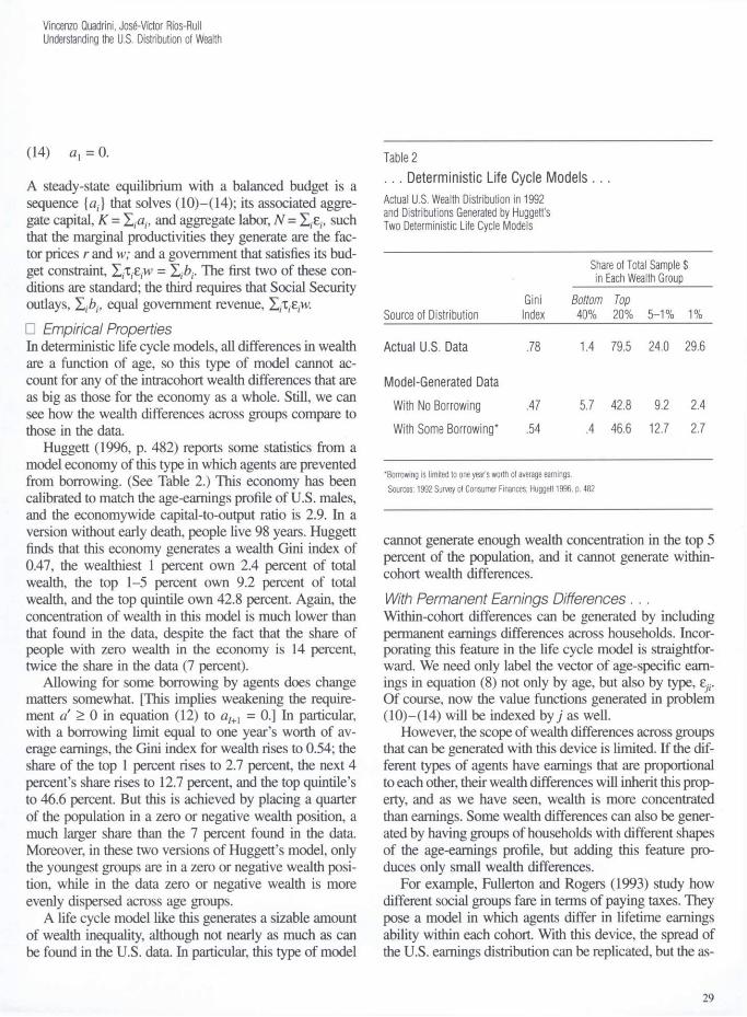
(14) ax = 0. A steady-state equilibrium with a balanced budget is a sequence {at} that solves (10)—(14); its associated aggre-gate capital, K = X-a,-, and aggregate labor, N = such that the marginal productivities they generate are the fac-tor prices r and w; and a government that satisfies its bud-get constraint, X/C v̂v = The first two of these con-ditions are standard; the third requires that Social Security outlays, X/b/, equal government revenue, E/C^vv. • Empirical Properties In deterministic life cycle models, all differences in wealth are a function of age, so this type of model cannot ac-count for any of the intracohort wealth differences that are as big as those for the economy as a whole. Still, we can see how the wealth differences across groups compare to those in the data.

Huggett (1996, p. 482) reports some statistics from a model economy of this type in which agents are prevented from borrowing. (See Table 2.) This economy has been calibrated to match the age-earnings profile of U.S. males, and the economywide capital-to-output ratio is 2.9. In a version without early death, people live 98 years. Huggett finds that this economy generates a wealth Gini index of 0.47, the wealthiest 1 percent own 2.4 percent of total wealth, the top 1-5 percent own 9.2 percent of total wealth, and the top quintile own 42.8 percent. Again, the concentration of wealth in this model is much lower than that found in the data, despite the fact that the share of people with zero wealth in the economy is 14 percent, twice the share in the data (7 percent).

Allowing for some borrowing by agents does change matters somewhat. [This implies weakening the require-ment a > 0 in equation (12) to aI+l = 0.] In particular, with a borrowing limit equal to one year's worth of av-erage earnings, the Gini index for wealth rises to 0.54; the share of the top 1 percent rises to 2.7 percent, the next 4 percent's share rises to 12.7 percent, and the top quintile's to 46.6 percent. But this is achieved by placing a quarter of the population in a zero or negative wealth position, a much larger share than the 7 percent found in the data. Moreover, in these two versions of Huggett's model, only the youngest groups are in a zero or negative wealth posi-tion, while in the data zero or negative wealth is more evenly dispersed across age groups.

A life cycle model like this generates a sizable amount of wealth inequality, although not nearly as much as can be found in the U.S. data. In particular, this type of model

Table 2 . . . Deterministic Life Cycle Models . . . Actual U.S. Wealth Distribution in 1992 and Distributions Generated by Huggett's Two Deterministic Life Cycle Models

Share of Total Sample $ in Each Wealth Group

Gini Bottom Top Source of Distribution Index 40% 20% 5-1% 1%

Actual U.S. Data .78 1.4 79.5 24.0 29.6

Model-Generated Data With No Borrowing .47 5.7 42.8 9.2 2.4 With Some Borrowing* .54 .4 46.6 12.7 2.7

*Borrowing is limited to one year's worth of average earnings. Sources: 1992 Survey of Consumer Finances; Huggett 1996, p. 482

cannot generate enough wealth concentration in the top 5 percent of the population, and it cannot generate within-cohort wealth differences. With Permanent Earnings Differences . . . Within-cohort differences can be generated by including permanent earnings differences across households. Incor-porating this feature in the life cycle model is straightfor-ward. We need only label the vector of age-specific earn-ings in equation (8) not only by age, but also by type, e;7. Of course, now the value functions generated in problem (10)—(14) will be indexed by j as well.

However, the scope of wealth differences across groups that can be generated with this device is limited. If the dif-ferent types of agents have earnings that are proportional to each other, their wealth differences will inherit this prop-erty, and as we have seen, wealth is more concentrated than earnings. Some wealth differences can also be gener-ated by having groups of households with different shapes of the age-earnings profile, but adding this feature pro-duces only small wealth differences.

For example, Fullerton and Rogers (1993) study how different social groups fare in terms of paying taxes. They pose a model in which agents differ in lifetime earnings ability within each cohort. With this device, the spread of the U.S. earnings distribution can be replicated, but the as-

29

sociated distribution of wealth does not generate a thick enough upper tail. To generate a wealth distribution con-sistent with the data,7 Fullerton and Rogers (1993) impose bequests as a constraint on the problem of the agents. More precisely, in their model, agents receive a certain size of bequest, indexed by type j, and have to leave the same size of bequest to their descendants (appropriately adjusted for population and productivity growth). The size of the be-quest used is obtained from Menchik and David (1982). The degree of concentration generated by this procedure is not endogenous, but is imposed in the calibration stage. Therefore, this approach does not help us understand what the factors are that underlie the wealth concentration. . . . And Precautionary Savings We turn now to life cycle models which include a precau-tionary motive for saving (in a very similar fashion to that posed in the dynastic model). In these stochastic models, uninsurable idiosyncratic shocks are self-insured by accu-mulating more wealth than that held for pure life cycle reasons.

Adding uninsurable risk to the life cycle model is quite simple. Earnings are affected by a shock 5 that changes the per period endowment of efficiency units of labor. This shock follows a Markov process with transition prob-ability matrix r[s'|s].8 The problem of the agent is now (15) vffca) = maxca, U(c) + p£{v/+1(sV)|*} subject to (16) a(l+r) -1- swe^l-T,) + bx? = c + a with v/+1 = 0, ax = 0, and a/+1 > 0. The solution to this problem is a = The existence of uninsurable risk implies that agents of the same age will have different wealth if they have had different earnings histories. The different properties of the agents can again be summarized with the aid of a measure x that describes the size of groups of people in each age-wealth-earnings group. Now aggregate capital in the economy is given by K - J/5A a dx.

Here, as in the dynastic model, a steady state requires that the agents solve their maximization problem, that fac-tor prices be marginal productivities, that the government balance its budget, (17) f b.dhC = f M fT dx*

Jl,S,A Jl,S,A and that the economy not change over time;9 that is, given

today's measure x*, the decisions of the agents replicate that measure tomorrow: (18) x*(/0,S0A)

The first two of those conditions are standard. The third requires that total Social Security payments, given by the left side of (17), equal the taxes levied by the government, the right side of (17). Finally, the fourth condition, that the economy not change over time, is a steady-state condition identical, except for the role played by age, to that in (5). • Empirical Properties With Earnings Uncertainty In life cycle models with earnings uncertainty, differences in wealth are a function partly of age and partly of the strings of good or bad times in people's lives. People of the same age can and, in general, will differ in the amount of wealth they hold. Now we can take a look at what life cycle models with idiosyncratic earnings uncertainty imply with respect to the distribution of wealth and how that compares with the data.

Huggett (1996) studies the properties of the distribution of wealth using an explicit general equilibrium version of a life cycle model with earnings uncertainty. The process for earnings is characterized by the sum of a deterministic life cycle component that changes with age and a stochas-tic component. The stochastic component has a standard deviation of 21 percent and an autocorrelation parameter of 0.96. Table 3 shows the Gini indexes and shares of total earnings and wealth in the United States and in this version of Huggett's model. We can see that despite the lower earnings concentration in Huggett's model, the Gini index for wealth is very close to that for wealth in the data. Unfortunately, the reason for such a high Gini is not that the richest people are as rich as in the data, but that the model has many more people with zero or negative wealth than in the data (24 percent versus 7 percent), and again, these people are basically young. Huggett (1996) also considers economies in which people face the pos-sibility of early death and economies in which people's

Generating such a distribution is important for Fullerton and Rogers' (1993) pur-pose of assessing the impact of taxation across different income, wealth, and age groups.

8Note that here, just as with the dynastic model, this notation can be used to refer to permanent differences in households.

9This condition is implicit in the definition of steady states for deterministic life cycle economies.

30

Vincenzo Quadrini, Jos-Victor Ros-Rull Understanding the U.S. Distribution of Wealth

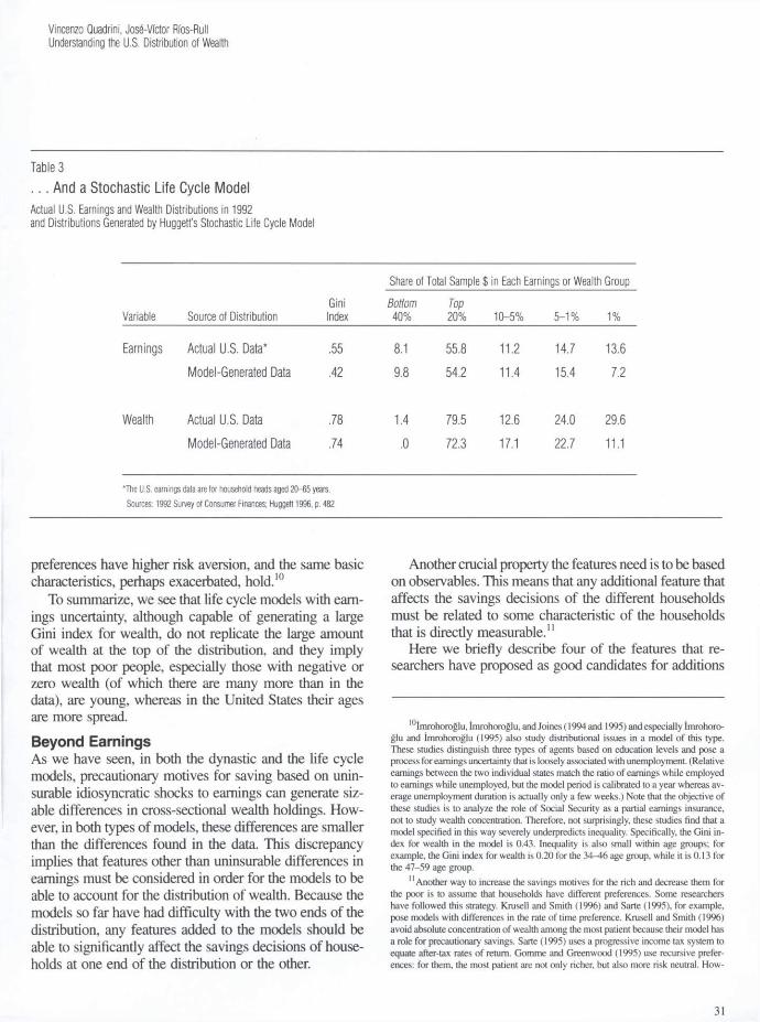
Table 3 . . . And a Stochastic Life Cycle Model Actual U.S. Earnings and Wealth Distributions in 1992 and Distributions Generated by Huggett's Stochastic Life Cycle Model

Share of Total Sample $ in Each Earnings or Wealth Group Gini Bottom Top

Variable Source of Distribution Index 40% 20% 10-5% 5-1% 1%

Earnings Actual U.S. Data* .55 8.1 55.8 11.2 14.7 13.6 Model-Generated Data .42 9.8 54.2 11.4 15.4 7.2

Wealth Actual U.S. Data .78 1.4 79.5 12.6 24.0 29.6 Model-Generated Data .74 .0 72.3 17.1 22.7 11.1

*The U.S. earnings data are for household heads aged 20-65 years. Sources: 1992 Survey of Consumer Finances; Huggett 1996, p. 482

preferences have higher risk aversion, and the same basic characteristics, perhaps exacerbated, hold.10

To summarize, we see that life cycle models with earn-ings uncertainty, although capable of generating a large Gini index for wealth, do not replicate the large amount of wealth at the top of the distribution, and they imply that most poor people, especially those with negative or zero wealth (of which there are many more than in the data), are young, whereas in the United States their ages are more spread. Beyond Earnings As we have seen, in both the dynastic and the life cycle models, precautionary motives for saving based on unin-surable idiosyncratic shocks to earnings can generate siz-able differences in cross-sectional wealth holdings. How-ever, in both types of models, these differences are smaller than the differences found in the data. This discrepancy implies that features other than uninsurable differences in earnings must be considered in order for the models to be able to account for the distribution of wealth. Because the models so far have had difficulty with the two ends of the distribution, any features added to the models should be able to significantly affect the savings decisions of house-holds at one end of the distribution or the other.

Another crucial property the features need is to be based on observables. This means that any additional feature that affects the savings decisions of the different households must be related to some characteristic of the households that is directly measurable.11

Here we briefly describe four of the features that re-searchers have proposed as good candidates for additions

I °imrohoroglu, Imrohoroglu, and Joines (1994 and 1995) and especially imrohoro-glu and Imrohoroglu (1995) also study distributional issues in a model of this type. These studies distinguish three types of agents based on education levels and pose a process for earnings uncertainty that is loosely associated with unemployment. (Relative earnings between the two individual states match the ratio of earnings while employed to earnings while unemployed, but the model period is calibrated to a year whereas av-erage unemployment duration is actually only a few weeks.) Note that the objective of these studies is to analyze the role of Social Security as a partial earnings insurance, not to study wealth concentration. Therefore, not surprisingly, these studies find that a model specified in this way severely underpredicts inequality. Specifically, the Gini in-dex for wealth in the model is 0.43. Inequality is also small within age groups; for example, the Gini index for wealth is 0.20 for the 34-46 age group, while it is 0.13 for the 47-59 age group.

II Another way to increase the savings motives for the rich and decrease them for the poor is to assume that households have different preferences. Some researchers have followed this strategy. Krusell and Smith (1996) and Sarte (1995), for example, pose models with differences in the rate of time preference. Krusell and Smith (1996) avoid absolute concentration of wealth among the most patient because their model has a role for precautionary savings. Sarte (1995) uses a progressive income tax system to equate after-tax rates of return. Gomme and Greenwood (1995) use recursive prefer-ences: for them, the most patient are not only richer, but also more risk neutral. How-

31

to the models. All of these features seem likely to work in the right direction of spreading out the wealth distribution. We don't know yet, however, what the quantitative impor-tance of any of them is or whether all of them are required to account for the facts of the U.S. wealth distribution. The Rich We start by looking at features that primarily affect the savings decisions of households that are quite wealthy. • Business Ownership One of these is business ownership. Diaz-Gimenez, Qua-drini, and Rios-Rull (in this issue, Table 9) report earnings, income, and wealth for both the self-employed and work-ers in the data. An important feature of these data is that entrepreneurs' wealth is almost five times that of workers (which puts the average entrepreneur in the top 10 percent of the wealth distribution) while the earnings of entrepre-neurs are less than double those of workers. This observa-tion suggests that entrepreneurs have different motivations for saving than workers do.

To properly model entrepreneurship, some departures from die standard model with uninsurable earnings risk must be made. The key role is played by imperfections in capital markets. Specifically, the following features are, we think, required:

• The rates of return of borrowing and lending are dif-ferent due to costly intermediation. This provides en-trepreneurs with a savings motive which other house-holds do not have: entrepreneurs face a higher rate of return.

• Agency problems require entrepreneurs to have a con-siderable amount of equity in their businesses. This issue, together with minimum size requirements in the operation of businesses, requires entrepreneurs to be relatively wealthy even before they open shop. Thus, it gives a further motive to save for those whose asset holdings are not far from the threshold required to be-come an entrepreneur.

• Entrepreneurs are not ex ante different from other types of agents. Entrepreneurs simply choose to en-gage in different activities than other agents due to the circumstances in which they get involved. In other words, every agent is a potential entrepreneur.

Quadrini (1997) follows these insights by constructing a general equilibrium model in which agents decide in each period whether or not to run a business. In Qua-

drini's model, running a business requires a certain mini-mum stock of capital, but imperfections in the financial markets prevent the entrepreneur from borrowing all the needed funds. Furthermore, the income generated by the project is quite variable.

Three features are particularly important in character-izing the equilibrium of this model economy: the presence of borrowing constraints, which has the effect of selecting entrepreneurs among richer families; the existence of a higher cost of external finance, which induces people who are entrepreneurs to accumulate more wealth in order to save on this cost; and the risk associated with business ac-tivities (higher than that associated with labor earnings), which provides entrepreneurs with an additional motive to increase their precautionary savings. Hence, Quadrini's model generates more inequality than does a similar mod-el without entrepreneurs. In a calibrated version of the dy-nastic model with earnings uncertainty (which we saw is not good at generating high wealth concentration), the Gini index for wealth rises from 0.55 to 0.73 while the wealth of the top 1 percent of agents rises from 4 percent to 24 per-cent. This is accomplished without generating an excessive number of agents with negative wealth: the high interest rate paid for loans prevents agents from borrowing too much.

Modeling entrepreneurs explicitly is a promising line of research to understand the behavior of households in the right tail of the distribution, and it emphasizes the fact that earnings opportunities may be related to wealth hold-ings. Compared with people in other employment groups, entrepreneurs face a higher effective rate of return and the shocks to their earnings (given by matrix T) have a higher variance. These two effects tend to induce higher savings for agents with higher levels of assets, which is what we need models to do more of.

ever, justifying differences in preferences to account for the wealth distribution is hard because preferences are not observable and any wealth distribution can be accounted for in this way.

Another approach, that follows the work of Duesenberry (1949), is to have models in which households care about their relative wealth in ways that increase the return of being rich. In this vein, Cole, Mailath, and Postlewaite (1992) explore a mechanism that induces households to care in equilibrium about their relative performance in terms of assets. This mechanism thus provides an accumulation rationale for richer house-holds, in addition to increasing future consumption. In the work of Cole, Mailath, and Postlewaite (1992), a market failure in the form of a local externality in consumption is responsible for creating savings incentives that affect the ordering. Presumably, the environment can be chosen so that some properties of the wealth distribution of the model match those of the data. Concerns about relative wealth also have the problem of being based on unobservables.

32

Vincenzo Quadrini, Jose-Victor Rfos-Rull Understanding the U.S. Distribution of Wealth

• Increasing Asset Returns and Capital Gains The portfolio of wealthy households typically includes assets that yield higher returns than the assets of poorer households. The higher the rate of return, the more attrac-tive is delaying consumption, which gives the wealthy a motive for saving that poorer households do not have.

Higher rates of return on assets for high asset levels can be modeled by posing two savings technologies: one with low returns and no fixed costs (say, a savings ac-count) and another with high returns but certain fixed costs (in terms of resources, knowledge, or time). Includ-ing this feature in a model induces poor households to hold the low-return asset and rich households to hold the high-return asset.

Unfortunately, the existence of returns that increase with the level of assets implies certain technical difficul-ties in terms of solving the maximization problem of the household. The budget set is nonconvex, which implies that the first-order conditions are not sufficient. To avoid this technical problem, some preliminary work has been done by Castaneda, Draz-Gimenez, and Rros-Rull (1996). They study the distributional effects of tax changes using a stochastic process for the idiosyncratic shock that affects not only the process for earnings, but also that for the rate of return. Stochastic returns are posed in the form of oc-casional capital gains and losses. Castaneda, Draz-Gimenez, and Rros-Rull have found that stochastic capital gains are necessary to generate high levels of wealth concentration. The Poor We now turn to features that primarily affect the savings decisions of those households that are poor, or have low levels of wealth. We start with a brief description of what these features are and how they affect households, and then we describe two studies that have considered them. • The Features Guaranteed Minimum Consumption. The key rationale for savings that we have reviewed states that households save to prevent future drops in earnings from dramatically re-ducing their consumption. If the government has a policy that guarantees a certain minimum level of consumption, then those households that foresee that their consumption is likely to remain below the government set minimum have no incentive to accumulate assets. If these people do accumulate assets, and their earnings do drop, they will not receive what the government would otherwise have given them. In other words, this policy implies that for poor peo-ple, the effective tax rate on savings can be above 100 per-

cent. Consequently, once a household achieves a very low asset level, and if its earnings are not expected to grow much, the optimal strategy for that household may be to not accumulate assets and, rather, to remain poor forever.

Health and Marital Risk. As we have seen, the central source of risk in models of the wealth distribution is chang-es in earnings. To specify an earnings process, researchers have calibrated a common process for individual earnings. But that type of process is not the only one that can be used to describe earnings. Events such as long-term health deterioration (including that of family members) can have a dramatic effect on the well-being of the people involved without necessarily leading to large changes in measured earnings. This type of what is effectively a large risk which is only partially insurable might send many people into poverty (and at the same time increase the precautionary motive for saving of people who are not subject to these extreme circumstances).

The data also suggest another feature that can be ex-plicitly modeled and that is intimately related to earnings and wealth: people's marital status. As we can see in the work of Draz-Gimenez, Quadrini, and Rros-Rull (in this issue, Table 9), households of different marital status have dramatically different profiles for earnings, income, and wealth. For example, married couples have a wealth-to-income ratio of about 4, while singles with dependents have a ratio of only about 2.5. Also, note that singles with dependents fare much worse than married couples or even than singles without dependents. Bane and Ellwood (1986) find that 11 percent of all poverty spells are triggered by transition into female-headed families and that 38 percent of the women who make the transition from being married to being single parents fall into poverty. In addition, John-son and Skinner (1986) document that family income, par-ticularly for women, dramatically drops when people di-vorce. For obvious moral hazard reasons, changes in mar-ital status are uninsurable, and they constitute a particular form of risk that does not appear directly in individual earnings data. The explicit consideration of uninsurable changes in marital status should be important to character-ize households at the bottom of the wealth distribution, es-pecially among the middle-aged and young. • The Studies Hubbard, Skinner, and Zeldes (1995) consider a life cycle model similar to the one with precautionary savings de-scribed earlier, but they add consumption support policies and health risks.

33

In their formulation, the consumption support policy is modeled as a minimum level of consumption guaranteed by the government. Therefore, in addition to Social Secu-rity transfers bx, the budget constraint of the agents includes transfers T necessary to guarantee the minimum consump-tion level c. Health risks in this model take the form of a shock that requires expenditures of resources without pro-viding utility. In order to distinguish the earnings shock from the health shock, denote the former by sl and the lat-ter by s2. The two shocks are assumed to be jointly Markov with transition matrix T.

The budget constraint then becomes (19) a(\+r) + slwEi( 1-T,) + bt + T= s2 + c + d (20) T= max{0,c + s2 - a(l+r) - (1-x)slwei - bt}. This budget constraint provides very low incentives to save at low levels of wealth, since it means that for low realiza-tions of sl (recurrent unemployment) and for large realiza-tions of s2 (expensive illnesses), the government will ef-fectively confiscate all of the household's savings.

Hubbard, Skinner, and Zeldes (1995) point out that if the population is sorted into three education classes (no high school degree, a high school degree but no college degree, and at least a college degree), the implied age pro-files of wealth and earnings do not seem to be generated by the same type of maximization problem with linear budget constraints, since the no-high school group holds very low assets, particularly in the years before retirement, when assets held should be highest. Hubbard, Skinner, and Zeldes argue that this observation is due to the existence of means-tested government programs that provide a safety net for consumption in a world with significant uncertainty in earnings and medical expenditures. Hubbard, Skinner, and Zeldes fix the consumption floor c at $7,000 (in 1984 dollars) by assessing the properties of a variety of govern-ment welfare programs. Their measure of earnings uncer-tainty (the residual of the log of earnings that cannot be accounted for by demographic and education variables) follows a highly autocorrelated process (with an autocor-relation parameter of about 0.95 for the three education groups), and the standard deviation of the innovations is about 18 percent for the no-high school group, 16 percent for the high school group, and 13 percent for the college group. The measure of medical expenses uncertainty that this study uses has an autocorrelation parameter of 0.901 and a standard deviation of 42 percent for the no-high

school group and 39 percent for the high school and col-lege groups. Given the transfers structure assumed, the study abstracts from Social Security.

Hubbard, Skinner, and Zeldes (1995) are able to repli-cate some features of the data, such as the fractions within each education group that receive public assistance, with-out concentrating poverty in the youngest groups, an out-come that arises in other life cycle models. Hubbard, Skinner, and Zeldes (1995) do not report measures of con-centration because they are not interested in the whole distribution of wealth. But we can easily see how a model of this type could generate a large number of households with very little wealth for all age groups, one of the key properties of the data that we are interested in. Although this type of model does not have features that could gen-erate a concentration of wealth at the top of the distribution that is higher than those generated by other life cycle models, the model does seem to have promise for the bottom of the distribution.

Cubeddu and Rfos-Rull (1996) explicitly model chang-es in marital status as a source of risk. They pose a life cycle model with agents differing in sex, and they model marital status as an exogenous idiosyncratic shock that af-fects earnings and the size of the household. This shock follows a Markov process that generates a distribution of people across marital status that resembles the distribution in the data. In this model, agents and households are not the same thing. The model has single-agent and multi-agent households. Differences in marital status histories determine current differences in wealth. The key items to use in a model like this are the asset-splitting rules in the event of divorce, the maximizing problem that the house-hold solves, and the modeling of how consumption expen-ditures in multiperson households translate into consump-tion enjoyed by the different agents.

Cubeddu and Rfos-Rull (1996) use this model to assess the importance of changes in social habits, such as increas-es in divorce and illegitimacy rates in shaping aggregate savings, but this type of model can also be used to try to assess the role of marital status in shaping the distribution of wealth. In the equilibrium of their model (as in the data), the poorest households are those that consist of an unmar-ried person with dependents.

The marital status of the household and its associated savings decisions, perhaps also with government transfers, seem promising features to build into models in order to try to understand the low levels of wealth held by large numbers of households in middle-aged groups.

34

Vincenzo Quadrini, Jos6-Victor Rios-Rull Understanding the U.S. Distribution of Wealth

Conclusion We have reviewed some of the standard quantitative models of capital accumulation and heterogeneous agents, and we have examined their ability to replicate the main features of the wealth distribution observed in the U.S. da-ta. Most of these models are based on uninsurable idio-syncratic risks to households' earnings that introduce pre-cautionary savings as the main mechanism that generates differences in asset holdings. We have shown that these models can generate substantial differences in asset hold-ings, but they still fall short of accounting for the high con-centration of wealth observed in the U.S. data. We have discussed some other research that considers other features underlying the generation of wealth differences. This work points to the key role played by entrepreneurship, increas-ing returns on assets, government consumption support policies, and changes in health and marital status. While the study of these features has just begun, the results so far suggest that including the features in computable general equilibrium models will help the models account for the wealth differences across households observed in the data.

References

Abowd, John M., and Card, David. 1989. On the covariance structure of earnings and hours changes. Econometrica 57 (March): 411-45.

Aiyagari, S. Rao. 1994. Uninsured idiosyncratic risk and aggregate saving. Quarterly Journal of Economics 109 (August): 659-84.

Ando, Albert, and Modigliani, Franco. 1963. The "life cycle" hypothesis of saving: Aggregate implications and tests. American Economic Review 53 (March): 55-84.

Auerbach, Alan J., and Kotlikoff, Laurence J. 1987. Dynamic fiscal policy. New York: Cambridge University Press.

Bane, Mary Jo, and Ellwood, David T. 1986. Slipping into and out of poverty: The dynamics of spells. Journal of Human Resources 21 (Winter): 1-23.

Bewley, Truman F. 1984. Notes on stationary equilibrium with a continuum of inde-pendently fluctuating consumers. Manuscript. Yale University.

Castaneda, Ana; Dfaz-Gimenez, Javier; and Rfos-Rull, Jose-Victor. 1996. A general equilibrium analysis of progressive income taxation: Quantifying the trade-offs. Manuscript. Federal Reserve Bank of Minneapolis.

. 1997. Unemployment spells, cyclically moving factor shares and income distribution dynamics. Manuscript. Federal Reserve Bank of Minneapolis.

Chatteijee, Satyajit. 1994. Transitional dynamics and the distribution of wealth in a neoclassical growth model. Journal of Public Economics 54 (May): 97-119.

Clarida, Richard H. 1990. International lending and borrowing in a stochastic, sta-tionary equilibrium. International Economic Review 31 (August): 543-58.

Clark, Kim B., and Summers, Lawrence H. 1981. Demographic differences in cyclical employment variation. Journal of Human Resources 16 (Winter): 61-79.

Cole, Harold L.; Mailath, George J.; and Postlewaite, Andrew. 1992. Social norms, savings behavior, and growth. Journal of Political Economy 100 (December): 1092-125.

Constantinides, George M., and Duffie, Darrell. 1996. Asset pricing with heterogeneous consumers. Journal of Political Economy 104 (April): 219-40.

Cubeddu, Luis Manuel, and Rfos-Rull, Jose-Victor. 1996. Marital risk and capital accu-mulation. Manuscript. University of Pennsylvania.

Duesenberry, James Stemble. 1949. Income, saving, and the theory of consumer be-havior. Cambridge, Mass.: Harvard University Press.

Fullerton, Don, and Rogers, Diane Lim. 1993. Who bears the lifetime tax burden? Washington, D.C.: Brookings Institution.

Gomme, Paul, and Greenwood, Jeremy. 1995. On the cyclical allocation of risks. Journal of Economic Dynamics and Control 19 (January-February): 91-124.

Heaton, John, and Lucas, Deborah J. 1996. Evaluating the effects of incomplete mar-kets on risk sharing and asset pricing. Journal of Political Economy 104 (June): 443-87.

Hubbard, R. Glenn; Skinner, Jonathan; and Zeldes, Stephen P. 1995. Precautionary sav-ing and social insurance. Journal of Political Economy 103 (April): 360-99.

Huggett, Mark. 1993. The risk-free rate in heterogeneous-agents, incomplete-insurance economies. Journal of Economic Dynamics and Control 17 (September-No-vember): 953-69.

. 1995. The one-sector growth model with idiosyncratic shocks. Dis-cussion Paper 105. Institute for Empirical Macroeconomics (Federal Reserve Bank of Minneapolis).

. 1996. Wealth distribution in life-cycle economies. Journal of Monetary Economics 38 (December): 469-94.

imrohoroglu, Ay§e, and imrohoroglu, Selahattin. 1995. Fiscal policy and the distribu-tion of wealth. Manuscript. University of Southern California.

imrohoroglu, Ay§e; Imrohoroglu, Selahattin; and Joines, Douglas H. 1994. Effect of tax-favored retirement accounts on capital accumulation and welfare. Manu-script. University of Southern California.

. 1995. A life cycle analysis of Social Security. Economic Theory 6 (June): 83-114.

Johnson, William R., and Skinner, Jonathan. 1986. Labor supply and marital sep-aration. American Economic Review 76 (June): 455-69.

Krusell, Per, and Smith, Anthony A., Jr. 1996. Income and wealth heterogeneity in the macroeconomy. Manuscript. University of Rochester.

Kydland, Finn E. 1984. Labor-force heterogeneity and the business cycle. Carnegie-Rochester Conference Series on Public Policy 21 (Autumn): 173-208.

Laitner, John P. 1979. Bequests, golden-age capital accumulation and government debt. Economica 46 (November): 403-14.

. 1992. Random earnings differences, lifetime liquidity constraints, and altruistic intergenerational transfers. Journal of Economic Theory 58 (Decem-ber): 135-70.

Menchik, Paul L., and David, Martin. 1982. The incidence of a lifetime consumption tax. National Tax Journal 35 (June): 189-203.

Quadrini, Vincenzo. 1997. Entrepreneurship, saving, and social mobility. Discussion Paper 116. Institute for Empirical Macroeconomics (Federal Reserve Bank of Minneapolis).

Rfos-Rull, Jose-Victor. 1993. Working in the market, working at home, and the acqui-sition of skills: A general-equilibrium approach. American Economic Review 83 (September): 893-907.

. 1995. Models with heterogeneous agents. In Frontiers of business cycle research, ed. Thomas F. Cooley, pp. 98-125. Princeton, N.J.: Princeton Univer-sity Press.

Samuelson, Paul A. 1958. An exact consumption-loan model of interest with or with-out the social contrivance of money. Journal of Political Economy 66 (Decem-ber): 467-82.

Sarte, Pierre-Daniel G. 1995. Progressive taxation and income inequality in dynamic competitive equilibrium. Manuscript. University of Rochester.

36