ALGORITHMS - BASICSYoung-Min Kang DEPT. GAME ENG., TONGMYONG UNIV., BUSAN, KOREA.

ALGORITHM

• “step-by-step” procedure for calculation

• input/output

• simple and clear

• finite

• executable

ALGORITHM ANALYSIS

• Asymptotic analysis

• analysing the limiting behaviours of functions

!

• the terms and are insignificant when n is very large

• f(n) is asymptotically equivalent to

• big-Oh, big-Omega, big-Theta

f(n) = n3 + 20n2 + 10n

20n2 10n

n3

f(n) = O(g(n) : f is bounded above by g

f(n) = ⌦(g(n)) : f is bounded below by g

f(n) = ⇥(g(n)) : f is bounded both above and below by g

upper bound

lower bound

BASIC DATA STRUCTURES

• array vs. linked list

• random access (time)

• array

• memory efficiency (space)

• linked list

LINKED LIST STRUCTURES

• singly linked list

• 1 node 1 link (next)

• doubly linked list

• 1 node 2 links (prev. and next)

• commonly used data

• head/tail pointers

BASIC DATA STRUCTURES

• Stack

• Last in, First out.

• data

• top: index

• array: stacked data

• operations

• push

• pop

BASIC DATA STRUCTURES

• Queue

• First in, First out.

• data

• front, rear: indices

• array: queued data

• operations

• add

• remove rear

add remove

TREES

• Graph G = {V, E}

• a set of vertices V and edges E

!

!

• Tree

• acyclic graph

TREES

• rooted or not?

• rooted tree

• hierarchical structureroot

HIERARCHICAL TREE

• 1 root

• multiple children for each node

• n = maximum number of children

• n-ary tree

• binary tree

• maximum number of children = 2

• level, height…

level 1

level 2

level 3

height of the node 10 = 2

height of the root = tree height

SORTING - SELECTION SORT

• list L = { sorted sublist L(+), unsorted sublist L(-) }

• initialisation: L = L(+)L(-)

• L(+) = nil

• L(-) = L

• Loop:

• find “min” in L(-), swap “min” and the 1st element of L(-)

• move the 1st element of L(-) to L(+)

• repeat this loop until L(+)=L

L(+)

L(-)

SORTING - BUBBLE SORT

• list L = { sorted sublist L(+), unsorted sublist L(-) }

• initialisation: L = L(-)L(+)

• L(-) = L

• L(+) = nil

• Loop:

• from left to right in L(-)

• compare two adjacent items and sort them

• the biggest item will be moved to the right end

• move the right-most element of L(-) to L(+)

• repeat this loop until L(+)=L

L(-) L(+) = 0

max will be here

L(-) L(-)

compare

compare

compare

...

SORTING - INSERTION SORT

• list L = { sorted sublist L(+), unsorted sublist L(-) }

• initialisation: L = L(+)L(-)

• L(+) = nil

• L(-) = L

• Loop

• take the 1st element of L(-)

• find the proper location in L(+), and insert it

• repeat this loop until L(+)=L

WHICH ONE IS BETTER?

• average time complexity

!

• almost-sorted list

• insertion sort works better

• because “proper location” can be quickly found

• in many cases

• “almost-sorted” lists are given (collision detection…)

• insertion sort rather than bubble sort• http://http.developer.nvidia.com/GPUGems3/elementLinks/32fig01.jpg

O(n2)

QUICK SORT: A QUICKER SORT?

• Quick sort

• list L to be sorted

• pivot element: a item x in L

• L(-): list of items less than x

• L(+): list of items greater than x

• algorithm

• select x in L

• partition L into L(-), x, L(+)

• recursive calls, one with L(-) and another with L(+)

HOW QUICK IS ‘QUICK SORT’?

• If you are lucky

• pivot divides the list evenly

• recursive call depth = lgn

• O(n) tasks for every level of the recursive call tree

• overall time complexity:

• When you’re down on your luck (already sorted list)

• pivot has the minimum or the maximum value

• O(n) recursive calls

• overall time complexity:

• Average:O(n lg n)

O(n lg n)

O(n2)

MERGE SORT - GUARANTEED

• algorithm

• Loop 1:

• evenly divide all lists

• repeat Loop 1 until all the lists are atomic

• Loop 2:

• merge adjacent lists

• repeat Loop 2 until we have only 1 list

O(n lg n)

SEARCH

• Sequential search

• O(n)

• more efficient methods are needed

• self-organising list

• frequently accessed items are moved to the front area

• you are not going to be lucky forever

BINARY SEARCH

• Rules

• your key: k

• you know value v at i: array[i] = v

• if k=v you found it

• if k>v the left part of array[i] can be ignored

• if k<v the right part can be ignored

• Algorithm

• 1. compare key and the middle of the list

• 2.

• if matched return the index of the middle

• if not matched remove the left or right from the middle in accordance with the rule above rules

• 3. goto 1 while the list is remained

BINARY SEARCH TREE

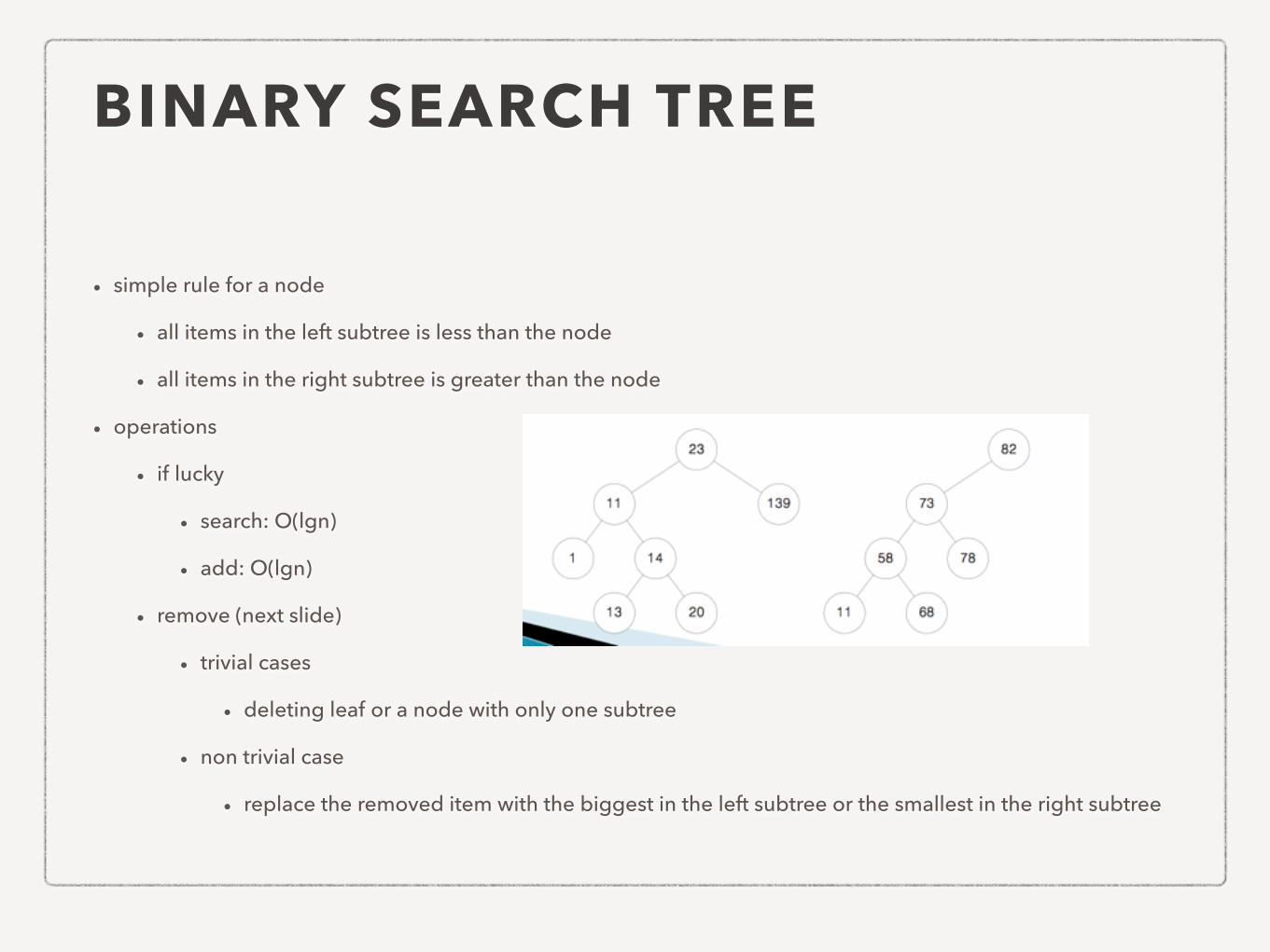
• simple rule for a node

• all items in the left subtree is less than the node

• all items in the right subtree is greater than the node

• operations

• if lucky

• search: O(lgn)

• add: O(lgn)

• remove (next slide)

• trivial cases

• deleting leaf or a node with only one subtree

• non trivial case

• replace the removed item with the biggest in the left subtree or the smallest in the right subtree

BST NODE REMOVAL

• Delete x

• if it’s a leaf

• just remove it

• internal node case 1

• if it has only one subtree

• link its parent and child

• internal node case 2

• if it has two subtrees

• find the min in the right subtree

• copy ‘min’ to x

• recursively delete ‘min’

2-3-4 TREE

• why it is needed

• BST can be skewed

• how to balance the tree: 2-3-4 tree

• 3 kinds of nodes

• 2 node

• 1 key with 2 links (binary tree node)

• 3 node

• 2 keys with 3 links

• 4 node

• 3 keys with 4 links Patrick Prosser, 2-3-4 trees and red-black tree, course slide, http://www.dcs.gla.ac.uk/~pat/52233/slides/234_RB_trees1x1.pdf

2-3-4 TREE: HOW IT WORKS

• find the leaf in the same way as BST

• if the leaf is 2- or 3-node, make it 3- or 4-node

• if the leaf is 4-node

• divide the 4-node into two 2-nodes

• move the middle element upwards

• put the new item

• chained 4-node division?

• pre-divide 4-nodes during the leaf search

• node removal: a bit complicated

2-3-4 tree is balanced! guaranteed O(lg n) search

Patrick Prosser, 2-3-4 trees and red-black tree, course slide, http://www.dcs.gla.ac.uk/~pat/52233/slides/234_RB_trees1x1.pdf

RED-BLACK TREE

• 2-3-4 tree: different node structures

• better implementation

• red-black tree

• 2-node

• 3-node

• 4-node

no consecutive red edges balanced if you just count the black edges

Patrick Prosser, 2-3-4 trees and red-black tree, course slide, http://www.dcs.gla.ac.uk/~pat/52233/slides/234_RB_trees1x1.pdf

RED-BLACK TREE

• insertion

• find leaf and add the new item

• mark red the edge from the parent to the new node

• keep “no consecutive red edges” rule

• cases

right rotation left rotation left-right double rotation right-left double rotation

promotion rule if incoming edges of p and its sibling are red, turn them black and mark the incoming edge of g red

Patrick Prosser, 2-3-4 trees and red-black tree, course slide, http://www.dcs.gla.ac.uk/~pat/52233/slides/234_RB_trees1x1.pdf

PRIORITY QUEUE - HEAP

• types

• max-heap: any of my descendants are less than me

• min-heap: any of my descendants are greater than me

• heap is a complete binary tree

• always balanced

• array implementation

• i-th node

• children: 2*i th and 2*i+1 th

• parent: �i

2

⌫

PRIORITY QUEUE - HEAP

• insert

PRIORITY QUEUE - HEAP

• delete

HASH

• hash function

• any function that maps data of arbitrary size to data of fixed size with slight differences in input data producing very big difference in output data (Wikipedia, http://en.wikipedia.org/wiki/Hash_function)

• hash functions are typically not invertible

• hash table

• data is stored as hash(data)-th element of the table

• collision

• if hash function is not perfect

• solution

• chaining

• open addressing

• linear probing, quadric probing, double hashing, random probing

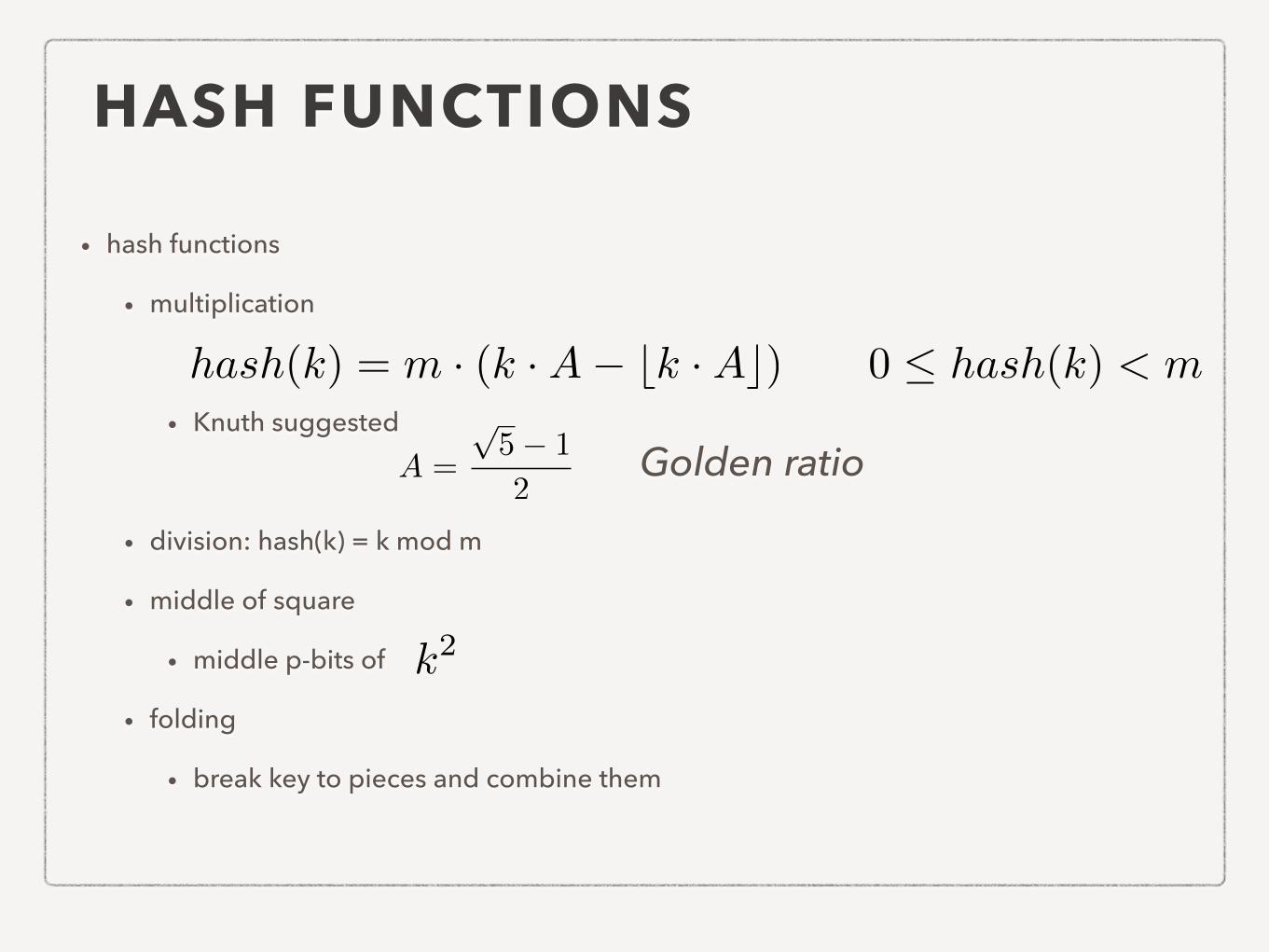
HASH FUNCTIONS

• hash functions

• multiplication

!

• Knuth suggested

!

• division: hash(k) = k mod m

• middle of square

• middle p-bits of

• folding

• break key to pieces and combine them

0 hash(k) < m

k2

A =

p5� 1

2

hash(k) = m · (k ·A� bk ·Ac)

Golden ratio

GRAPH

• graph G = {V,E}

• V: set of vertices

• E: set of edges linking two vertices

• adjacent

• if two nodes are connected with an edge

• data structures for graph

• adjacent matrix or adjacent list

• graph types

• directed or undirected

• weighted or non-weighted

undirected vs. directed

weighted vs. non-weighted

GRAPH TRAVERSAL

• Depth-first vs. Breadth-first search

• stack vs. queue

A

B

C

D

E

F

G

HI

DFSStack

[A] [AB] [ABC] [AB] [ABD] [ABDE] [ABDEF] [ABDE] [ABDEG] [ABDEGH] [ABDEG] [ABDGI]

Traversal: A, B, C, D, E, F, G, H, I

BFS

Queue

Traversal: A, B, C, D, E, G, F, H, I

[A] [B] [CD] [D] [EGH] [GHF] [HFI]

A

B

C

DE

F

G

HI

A

B

C

DE

F

G

H I

DFS tree

BFS tree

MINIMUM COST SPANNING TREE

• Greedy Algorithm

• Prim’s method

• two vertices sets: V, U

• select a node v0 and initialise V={v0}

• U = { all other vertices}

• find the minimum edge (v in V, u in U) that links V and U

• if it does not create a cycle, add u into V

• Kruskal’s method

• sort the edge list

• add edge in increasing order

• if it creates a cycle, throw it away

DIJKSTRA’S SHORTEST PATH

• single source - multiple destination

subgraph with vertices of which shortest path was found

subgraph with vertices of which shortes paths are not known yet

G

+

G

�

start

u : newly added vertex

d

+= 0

d

+u : found

v1

v2

vn

.

.

.

c1

c2

cn

d

�v2

d

�v1

d

�vn

initialisation

d

+start = 0

d

�vi =1

G

+= start

G

�= G� start

u = start

Loop

d

+u + ci < d

�vi ) d

�vi d

+u + ci

for all i

find minimum d

�v in G

�

add v into G

+, remove it from G

�

fix d

�v to be d

+v

u v

While G

�is not empty

STRING SEARCH RABIN-KARP METHOD• Rabin-Karp

• T: text with size of m characters

• p: pattern with n characters

• h = hash(p)

• hi: hash value of n-character substring of T starting at T[i]

• if h = hi, string “T[i]…T[i+n-1]” can be p

• i=0 to m-n

• Hash

hi =n�1X

j=0

T [i+ j] · 2n�1�j

hi+1 = hi � T [i] · 2n�1 + T [i+ n]

abcdefghijklmnopqrstuvwxyz

hash value = h1

hash value = h2

h2 = h1 � b · 210 +m

STRING SEARCH KNUTH-MORRIS-PRATT METHOD

text

pattern mismatch

1 character shift

naive approach

text

pattern mismatch

jump to the mismatched location?

we want...

ANY PROBLEM?

Sometimes we cannot jump that far... Why?

text

pattern mismatch

identical

”Jump Table” is required

border

STRING SEARCH BOYER-MOORE METHOD• right to left comparison

• bad character shift

• good suffix shifttext

pattern

mismatch

comparison direction

bad character

bad character shift

text

pattern

mismatch

comparison direction

good su�x

case 1

case 2

good su�x is found in the left

su�x of good su�x matches the prefix of pattern

DYNAMIC PROGRAMMING LONGEST COMMON SUBSEQUENCE

• subsequence

• a sequence derived from another sequence by deleting some elements without altering the order of the elements

• common subsequence

• G is common subsequence of X and Y iff G is a subsequence of both X and Y

• longest common subsequence

• optimal substructure!

Xi =< x1, x2, · · · , xi >

Yj =< y1, y2, · · · , yj >

|LCS(Xi, Yi)| =

0

@0 , if i = 0 or j = 0

|LCS(Xi�1, Yj�1)|+ 1 , if xi = yj

max(|LCS(Xi�1, Yj)|, |LCS(Xi, Yj�1)|) , if xi 6= yj and i, j > 0

1

A

PROBLEM SOLVING STRATEGIES

• Divide & Conquer

• Quick sort, Merge sort

• Greedy algorithms

• Optimal substructure

• Minimum cost spanning tree, shortest path

• easy to implement

• Dynamic Programming

• Optimal substructure

• solving big problem by breaking down into simple subproblems