Embed Size (px)
Citation preview
Tutorial 3
Inferential Statistics, Statistical Modelling & Survey Methods
(BS2506)
Pairach Piboonrungroj(Champ)
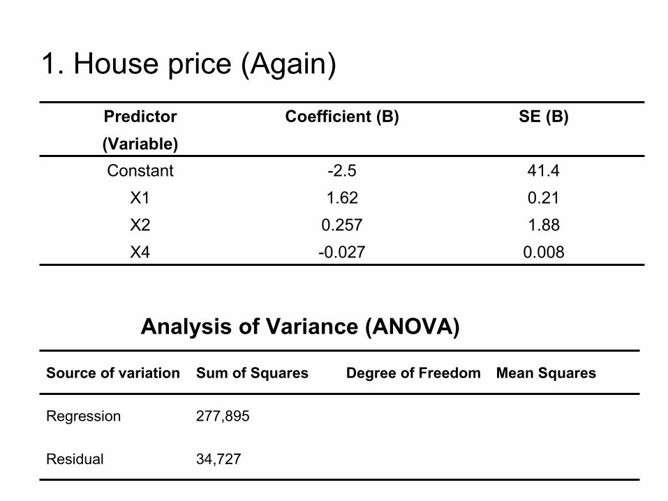
1. House price (Again)
Predictor
(Variable)
Coefficient (B) SE (B)
Constant -2.5 41.4
X1 1.62 0.21
X2 0.257 1.88
X4 -0.027 0.008
Source of variation Sum of Squares Degree of Freedom Mean Squares
Regression 277,895
Residual 34,727
Analysis of Variance (ANOVA)
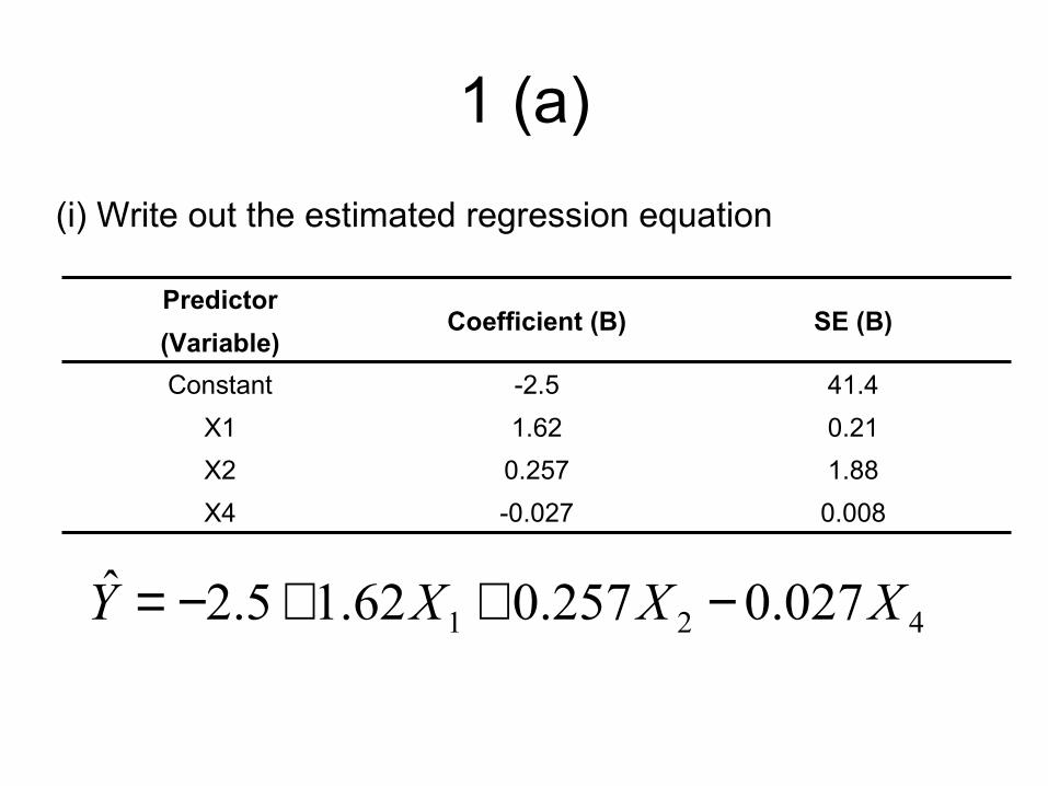
1 (a)
(i) Write out the estimated regression equation
421 027.0257.062.15.2ˆ XXXY −++−=
Predictor
(Variable)Coefficient (B) SE (B)
Constant -2.5 41.4
X1 1.62 0.21
X2 0.257 1.88
X4 -0.027 0.008
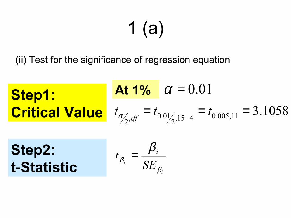
1 (a)
(ii) Test for the significance of regression equation
1058.311,005.0415,201.0,2
===−
tttdfα
01.0=αAt 1%Step1: Critical Value
Step2: t-Statistic i
i SEt i
ββ
β=
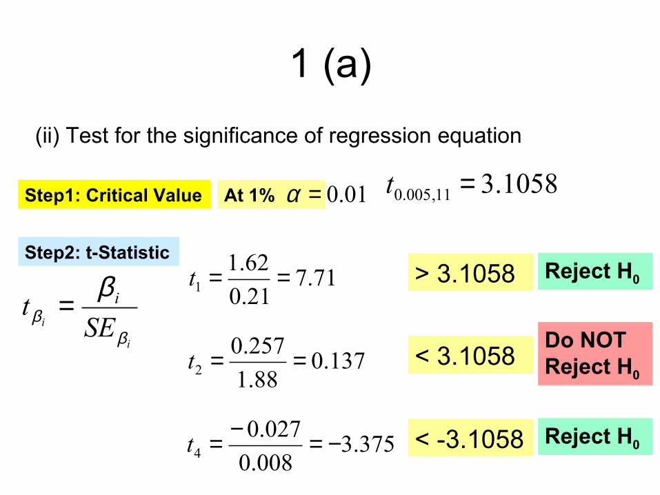
1 (a)
(ii) Test for the significance of regression equation
1058.311,005.0 =tAt 1%Step1: Critical Value
Step2: t-Statistic
i
i SEt i
ββ
β=
01.0=α
71.721.0
62.11 ==t
137.088.1
257.02 ==t
375.3008.0
027.04 −=−=t
Reject H0
Do NOTReject H0
Reject H0
> 3.1058
< 3.1058
< -3.1058
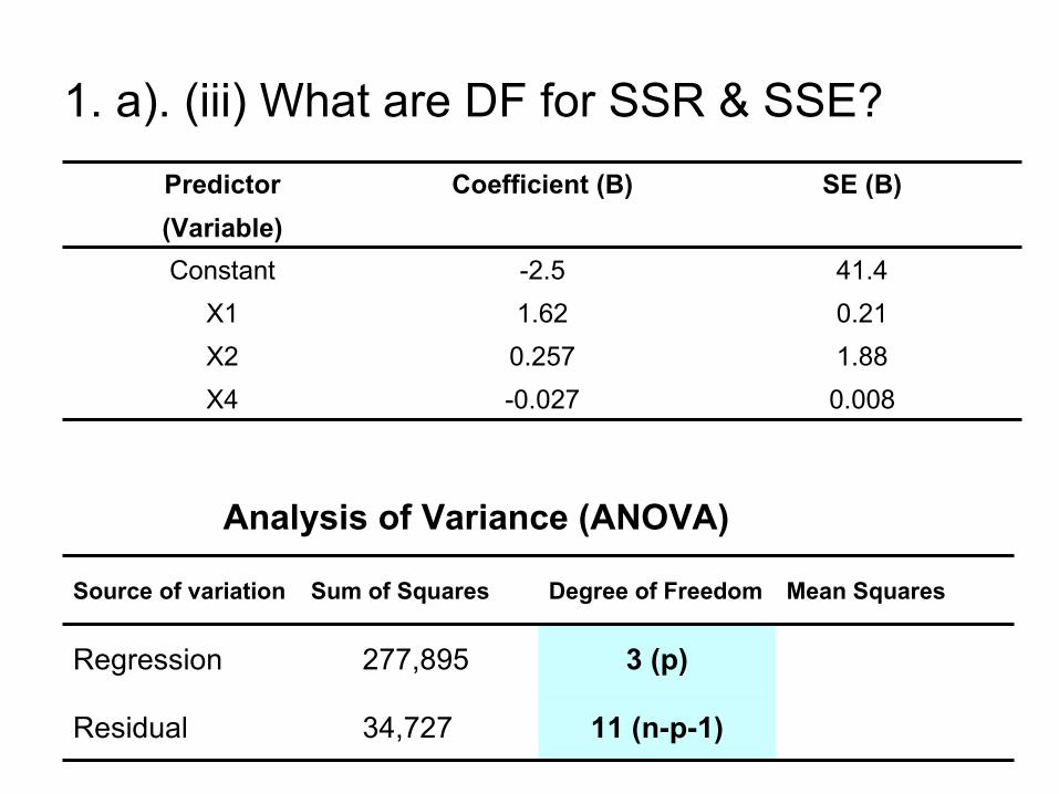
1. a). (iii) What are DF for SSR & SSE?
Predictor
(Variable)
Coefficient (B) SE (B)
Constant -2.5 41.4
X1 1.62 0.21
X2 0.257 1.88
X4 -0.027 0.008
Source of variation Sum of Squares Degree of Freedom Mean Squares
Regression 277,895 3 (p)
Residual 34,727 11 (n-p-1)
Analysis of Variance (ANOVA)
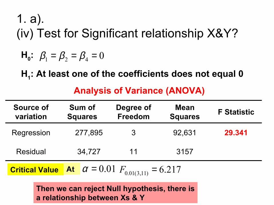
1. a). (iv) Test for Significant relationship X&Y?
Source of variation
Sum of Squares
Degree of Freedom
Mean Squares
F Statistic
Regression 277,895 3 92,631 29.341
Residual 34,727 11 3157
Analysis of Variance (ANOVA)
0421 === βββH0:
H1: At least one of the coefficients does not equal 0
217.6)11,3(01.0 =FAtCritical Value 01.0=α
Then we can reject Null hypothesis, there is a relationship between Xs & Y
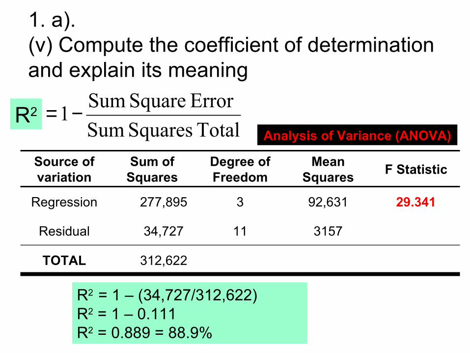
1. a). (v) Compute the coefficient of determination and explain its meaning
Source of variation
Sum of Squares
Degree of Freedom
Mean Squares
F Statistic
Regression 277,895 3 92,631 29.341
Residual 34,727 11 3157
TOTAL 312,622
Analysis of Variance (ANOVA)R2
R2 = 1 – (34,727/312,622)R2 = 1 – 0.111R2 = 0.889 = 88.9%
Total Squares Sum
Error Square Sum1−=
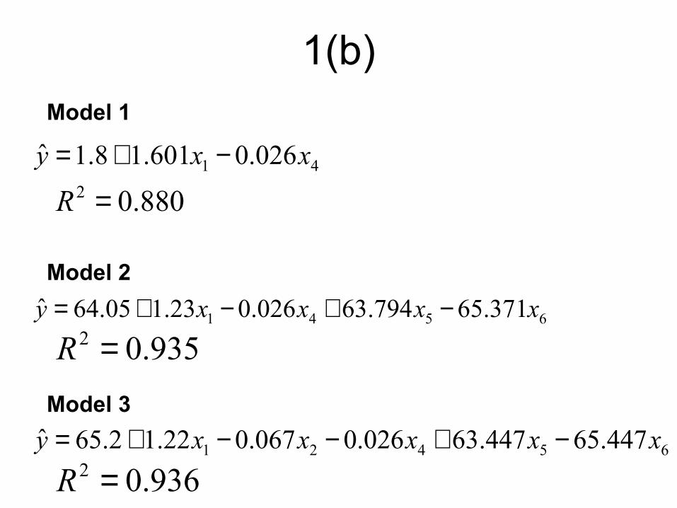
1(b)
41 026.0601.18.1ˆ xxy −+=
880.02 =R
Model 1
6541 371.65794.63026.023.105.64ˆ xxxxy −+−+=Model 2
935.02 =R
65421 447.65447.63026.0067.022.12.65ˆ xxxxxy −+−−+=Model 3
936.02 =R
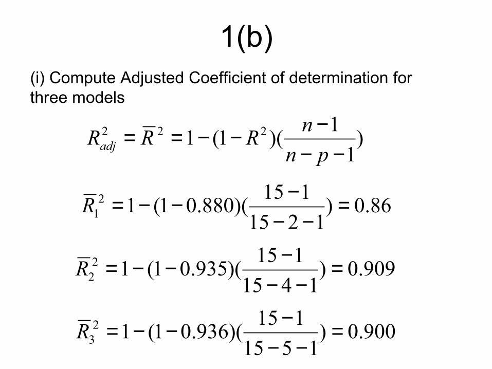
1(b)(i) Compute Adjusted Coefficient of determination for three models
)1
1)(1(1 222
−−−−−==pn
nRRRadj
86.0)1215
115)(880.01(12
1 =−−
−−−=R
909.0)1415
115)(935.01(12
2 =−−
−−−=R
900.0)1515
115)(936.01(12
3 =−−
−−−=R
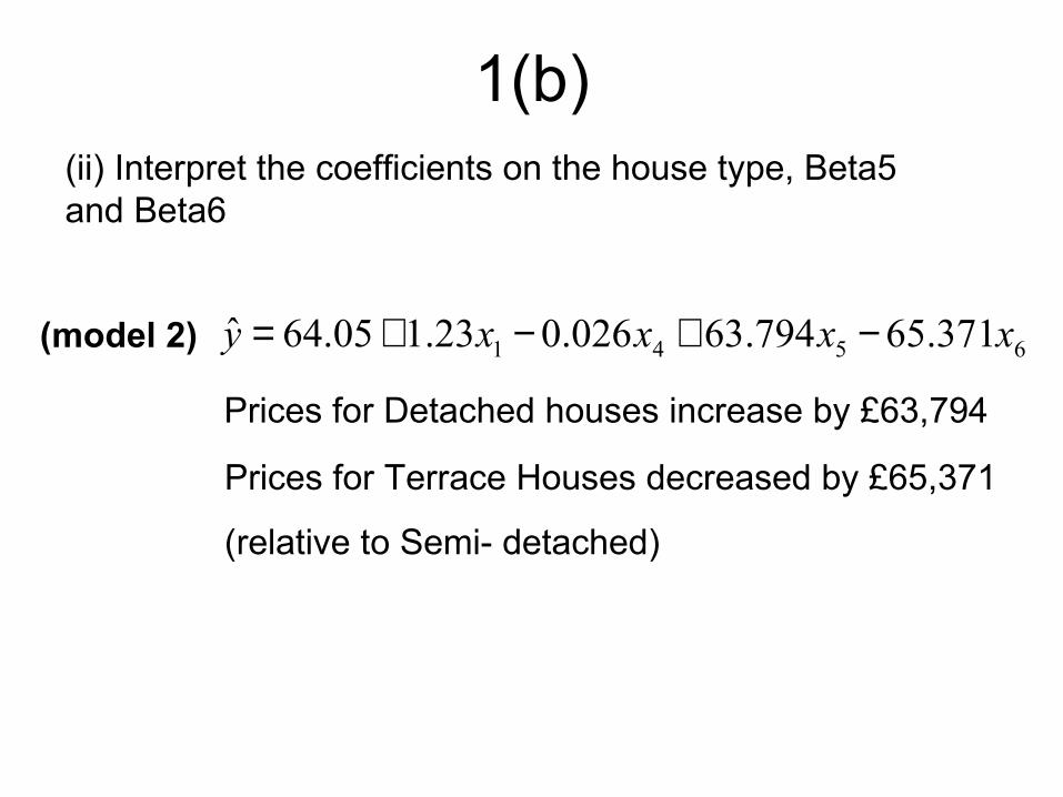
1(b)(ii) Interpret the coefficients on the house type, Beta5 and Beta6
Prices for Detached houses increase by £63,794
Prices for Terrace Houses decreased by £65,371
(relative to Semi- detached)
6541 371.65794.63026.023.105.64ˆ xxxxy −+−+=(model 2)
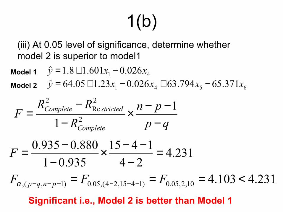
1(b)(iii) At 0.05 level of significance, determine whether model 2 is superior to model1
6541 371.65794.63026.023.105.64ˆ xxxxy −+−+=Model 2
41 026.0601.18.1ˆ xxy −+=Model 1
qp
pn
R
RRF
Complete
strictedComplete
−−−×
−−
= 1
1 2
2Re
2
231.424
1415
935.01
880.0935.0 =−
−−×−
−=F
231.4103.410,2,05.0)1415,24(,05.0)1,(, <=== −−−−−− FFF pnqpα
Significant i.e., Model 2 is better than Model 1
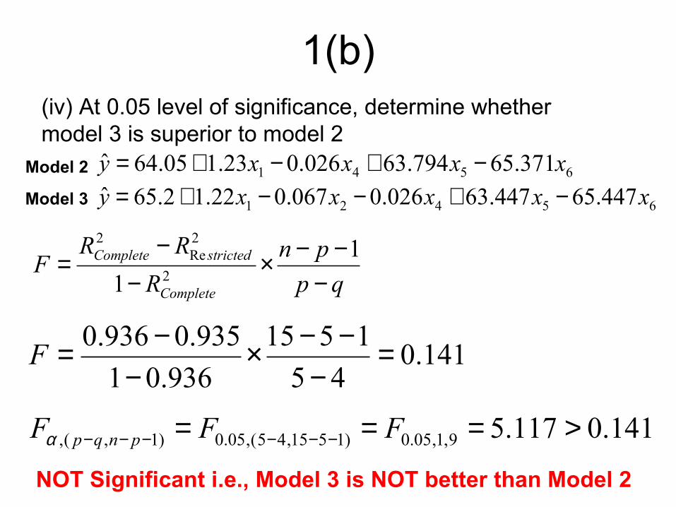
1(b)(iv) At 0.05 level of significance, determine whether model 3 is superior to model 2
6541 371.65794.63026.023.105.64ˆ xxxxy −+−+=Model 2
qp
pn
R
RRF
Complete
strictedComplete
−−−×
−−
= 1
1 2
2Re
2
141.045
1515
936.01
935.0936.0 =−
−−×−
−=F
141.0117.59,1,05.0)1515,45(,05.0)1,(, >=== −−−−−− FFF pnqpα
NOT Significant i.e., Model 3 is NOT better than Model 2
65421 447.65447.63026.0067.022.12.65ˆ xxxxxy −+−−+=Model 3
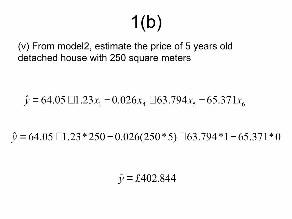
6541 371.65794.63026.023.105.64ˆ xxxxy −+−+=
0*371.651*794.63)5*250(026.0250*23.105.64ˆ −+−+=y
844,402£ˆ =y
1(b)(v) From model2, estimate the price of 5 years old detached house with 250 square meters
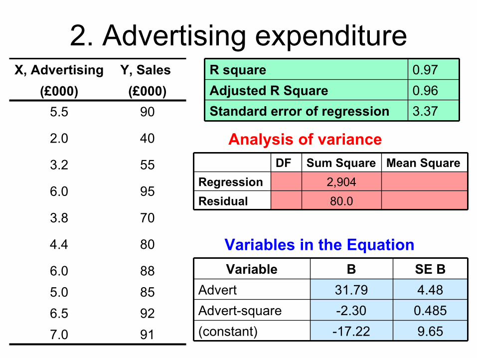
2. Advertising expenditureX, Advertising
(£000)
Y, Sales
(£000)
5.5 90
2.0 40
3.2 55
6.0 95
3.8 70
4.4 80
6.0
5.0
6.5
7.0
88
85
92
91
R square 0.97
Adjusted R Square 0.96
Standard error of regression 3.37
DF Sum Square Mean Square
Regression 2,904
Residual 80.0
Analysis of variance
Variables in the Equation
Variable B SE B
Advert 31.79 4.48
Advert-square -2.30 0.485
(constant) -17.22 9.65
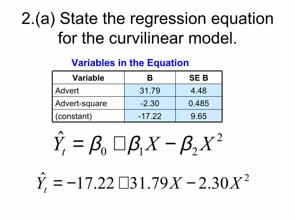
2.(a) State the regression equation for the curvilinear model.
230.279.3122.17ˆ XXYt −+−=
Variables in the Equation
Variable B SE B
Advert 31.79 4.48
Advert-square -2.30 0.485
(constant) -17.22 9.65
2210
ˆ XXYt βββ −+=
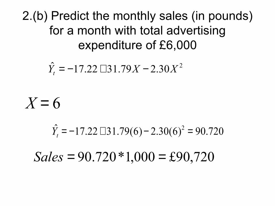
2.(b) Predict the monthly sales (in pounds) for a month with total advertising
expenditure of £6,000
230.279.3122.17ˆ XXYt −+−=
X = 6
Yt = −17.22 + 31.79(6)− 2.30(6)2 = 90.720
720,90£000,1*720.90 ==Sales
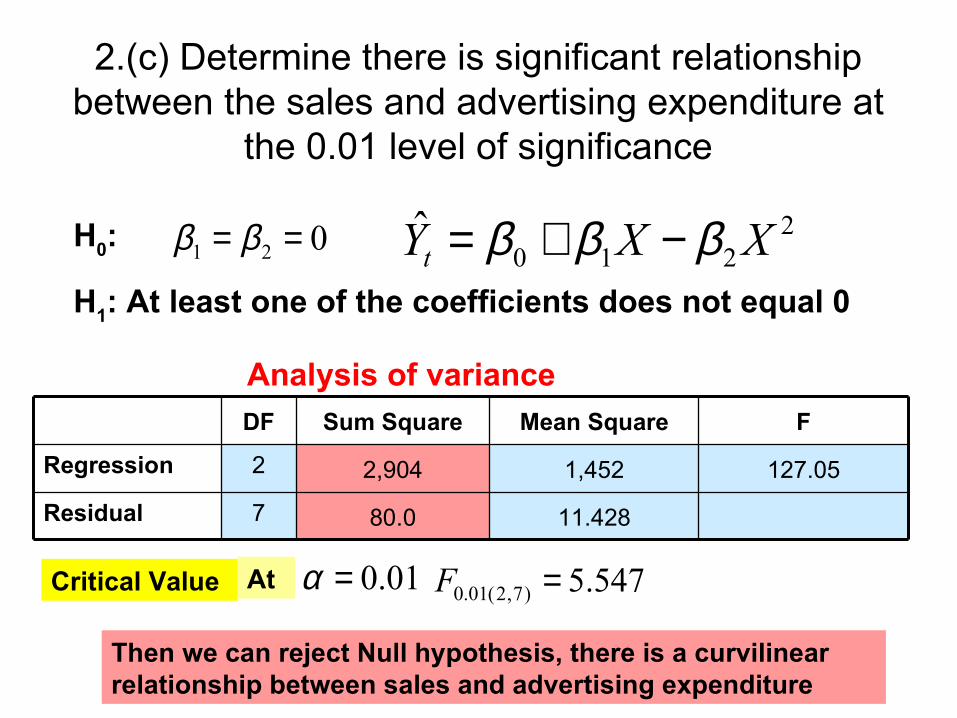
2.(c) Determine there is significant relationship between the sales and advertising expenditure at
the 0.01 level of significance
DF Sum Square Mean Square F
Regression 2 2,904 1,452 127.05
Residual 7 80.0 11.428
Analysis of variance
547.5)7,2(01.0 =FAtCritical Value 01.0=α
Then we can reject Null hypothesis, there is a curvilinear relationship between sales and advertising expenditure
021 == ββH0:
H1: At least one of the coefficients does not equal 0
2210
ˆ XXYt βββ −+=
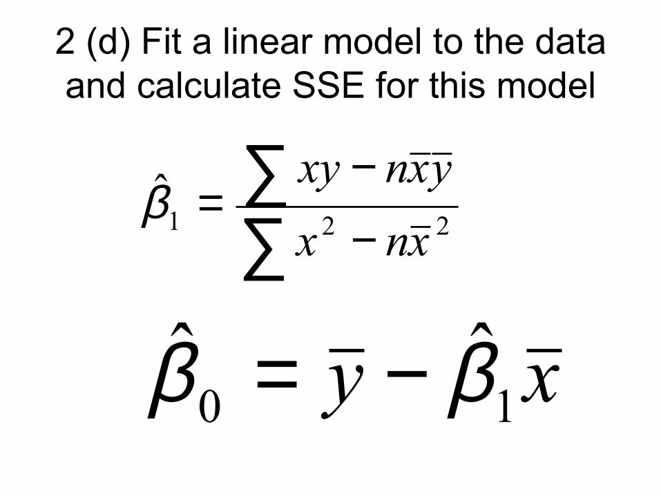
2 (d) Fit a linear model to the data and calculate SSE for this model
∑∑
−−
=221
ˆxnx
yxnxyβ
xy 10ˆˆ ββ −=

2 (d) Fit a linear model to the data and calculate SSE for this model
IDX
Advertising
Y
Sales
1 5.5 90
2 2 40
3 3.2 55
4 6 95
5 3.8 70
6 4.4 80
7 6 88
8 5 85
9 6.5 92
10 7 91

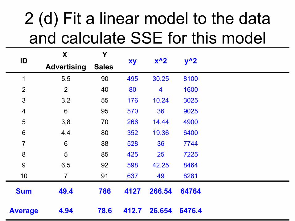
2 (d) Fit a linear model to the data and calculate SSE for this model
IDX
Advertising
Y
Sales xy x^2 y^2
1 5.5 90 495 30.25 8100
2 2 40 80 4 1600
3 3.2 55 176 10.24 3025
4 6 95 570 36 9025
5 3.8 70 266 14.44 4900
6 4.4 80 352 19.36 6400
7 6 88 528 36 7744
8 5 85 425 25 7225
9 6.5 92 598 42.25 8464
10 7 91 637 49 8281
Sum 49.4 786 4127 266.54 64764
Average 4.94 78.6 412.7 26.654 6476.4
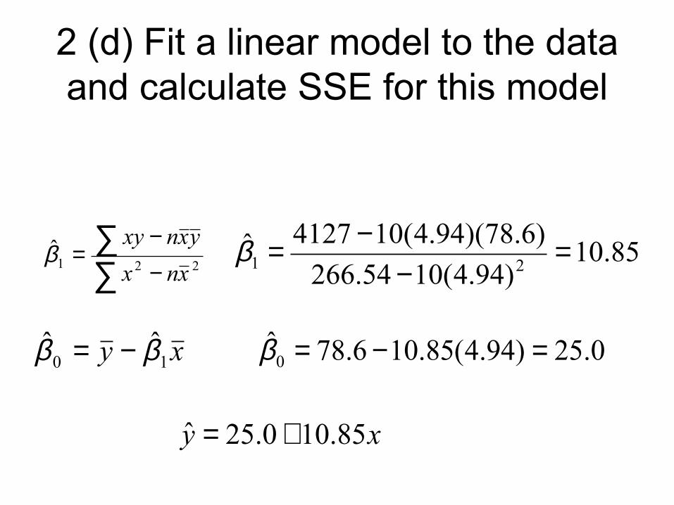
2 (d) Fit a linear model to the data and calculate SSE for this model
∑∑
−−
=221
ˆxnx
yxnxyβ 85.10
)94.4(1054.266
)6.78)(94.4(104127ˆ21 =
−−=β
xy 10ˆˆ ββ −= 0.25)94.4(85.106.78ˆ
0 =−=β
xy 85.100.25ˆ +=
2 (d) Fit a linear model to the data and calculate SSE for this model
IDX
Advertising
Y
Sales xy x^2 y^2
1 5.5 90 495 30.25 8100
2 2 40 80 4 1600
3 3.2 55 176 10.24 3025
4 6 95 570 36 9025
5 3.8 70 266 14.44 4900
6 4.4 80 352 19.36 6400
7 6 88 528 36 7744
8 5 85 425 25 7225
9 6.5 92 598 42.25 8464
10 7 91 637 49 8281
Sum 49.4 786 4127 266.54 64764
Average 4.94 78.6 412.7 26.654 6476.4

2 (d) Fit a linear model to the data and calculate SSE for this model
IDX
Advertising
Y
Sales xy x^2 y^2
predicted Y
1 5.5 90 495 30.25 8100 84.68
2 2 40 80 4 1600 46.70
3 3.2 55 176 10.24 3025 59.72
4 6 95 570 36 9025 90.10
5 3.8 70 266 14.44 4900 66.23
6 4.4 80 352 19.36 6400 72.74
7 6 88 528 36 7744 90.10
8 5 85 425 25 7225 79.25
9 6.5 92 598 42.25 8464 95.53
10 7 91 637 49 8281 100.95
Sum 49.4 786 4127 266.54 64764
Average 4.94 78.6 412.7 26.654 6476.4
XYt 85.1025ˆ +=
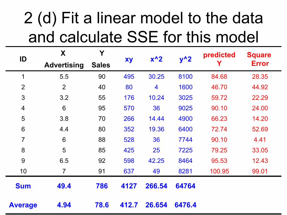
2 (d) Fit a linear model to the data and calculate SSE for this model
IDX
Advertising
Y
Sales xy x^2 y^2
predicted Y
Square Error
1 5.5 90 495 30.25 8100 84.68 28.35
2 2 40 80 4 1600 46.70 44.92
3 3.2 55 176 10.24 3025 59.72 22.29
4 6 95 570 36 9025 90.10 24.00
5 3.8 70 266 14.44 4900 66.23 14.20
6 4.4 80 352 19.36 6400 72.74 52.69
7 6 88 528 36 7744 90.10 4.41
8 5 85 425 25 7225 79.25 33.05
9 6.5 92 598 42.25 8464 95.53 12.43
10 7 91 637 49 8281 100.95 99.01
Sum 49.4 786 4127 266.54 64764
Average 4.94 78.6 412.7 26.654 6476.4
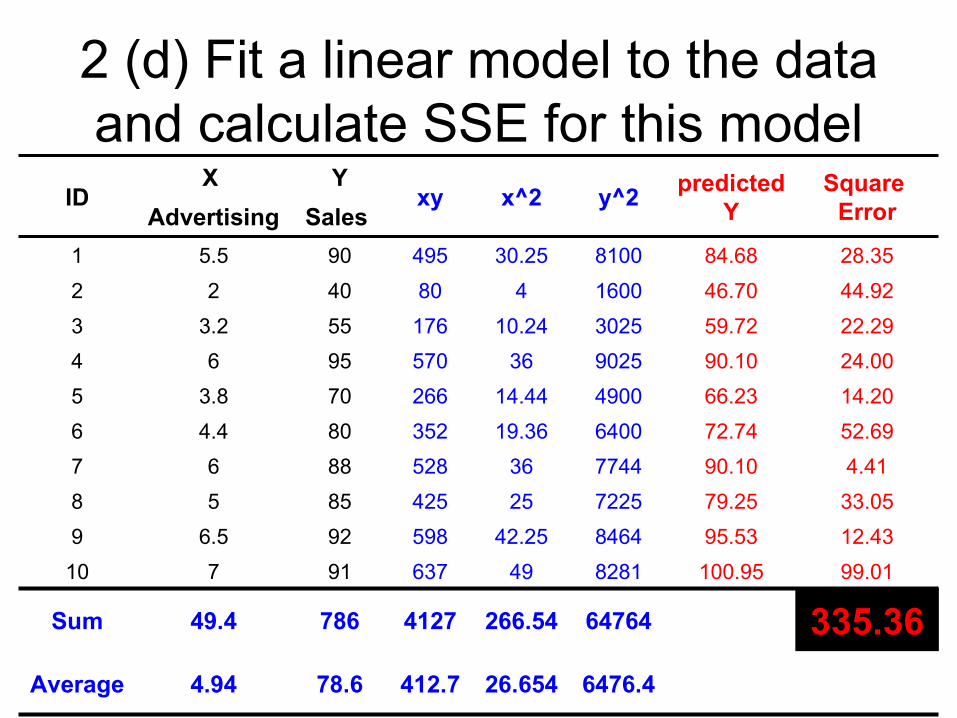
2 (d) Fit a linear model to the data and calculate SSE for this model
IDX
Advertising
Y
Sales xy x^2 y^2
predicted Y
Square Error
1 5.5 90 495 30.25 8100 84.68 28.35
2 2 40 80 4 1600 46.70 44.92
3 3.2 55 176 10.24 3025 59.72 22.29
4 6 95 570 36 9025 90.10 24.00
5 3.8 70 266 14.44 4900 66.23 14.20
6 4.4 80 352 19.36 6400 72.74 52.69
7 6 88 528 36 7744 90.10 4.41
8 5 85 425 25 7225 79.25 33.05
9 6.5 92 598 42.25 8464 95.53 12.43
10 7 91 637 49 8281 100.95 99.01
Sum 49.4 786 4127 266.54 64764 335.36
Average 4.94 78.6 412.7 26.654 6476.4
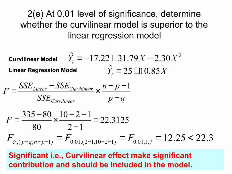
2(e) At 0.01 level of significance, determine whether the curvilinear model is superior to the
linear regression model
Linear Regression Model
Curvilinear Model
qp
pn
SSE
SSESSEF
rCurvilinea
rCurvilineaLinear
−−−×−= 1
3125.2212
1210
80
80335 =−
−−×−=F
3.2225.127,1,01.0)1210,12(,01.0)1,(, <=== −−−−−− FFF pnqpα
Significant i.e., Curvilinear effect make significant contribution and should be included in the model.
230.279.3122.17ˆ XXYt −+−=XYt 85.1025ˆ +=
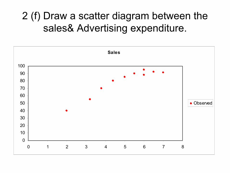
2 (f) Draw a scatter diagram between the sales& Advertising expenditure.
Sales
0
10
20
30
40
50
60
70
80
90
100
0 1 2 3 4 5 6 7 8
Observed
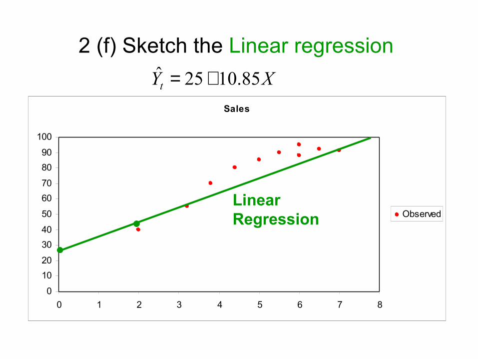
2 (f) Sketch the Linear regression
Sales
0
10
20
30
40
50
60
70
80
90
100
0 1 2 3 4 5 6 7 8
ObservedLinear Regression
XYt 85.1025ˆ +=
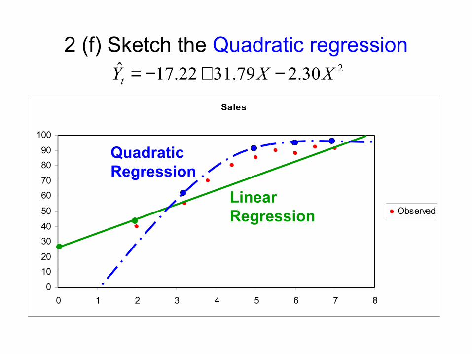
2 (f) Sketch the Quadratic regression
Sales
0
10
20
30
40
50
60
70
80
90
100
0 1 2 3 4 5 6 7 8
ObservedLinear Regression
Quadratic Regression
230.279.3122.17ˆ XXYt −+−=

Thank youDownload this Slides at
www.pairach.com/teaching
Q & A