decision tree in quantitative analysis

qwertyuiopasdfghjklzxcvbnmqwertyuiopasdfghjklzxcvbnmqwertyuiopasdfghjklzxcvbnmqwertyuiopasdfghjklzxcvbnmqwertyuiopasdfghjklzxcvbnmqwertyuiopasdfghjklzxcvbnmqwertyuiopasdfghjklzxcvbnmqwertyuiopasdfghjklzxcvbnmqwertyuiopasdfghjklzxcvbnmqwertyuiopasdfghjklzxcvbnmqwertyuiopasdfghjklzxcvbnmqwertyuiopasdfghjklzxcvbnmqwertyuiopasdfghjklzxcvbnmqwertyuiopasdfghjklzxcvbnmqwertyuiopasdfghjklzxcvbnmqwertyuiopasdfghjklzxcvbnmqwertyuiopasdfghjklzxcvbnmqwertyuiopasdfghjklzxcvbnmrtyuiopasdfghjklzxcvbnmqwertyuiopasdfghjklzxcvbnmqwertyuiopasdfghjklzxcvbnmqwertyuiopasdfghjklzxcvbnmqw

UNIT: - II

UNIT: - II

QTBD

I MBA I SEM

QISET COLLEGE @ K.V.RAMESH BABU

ASSISTANT PROFESSOR IN STATISTICS

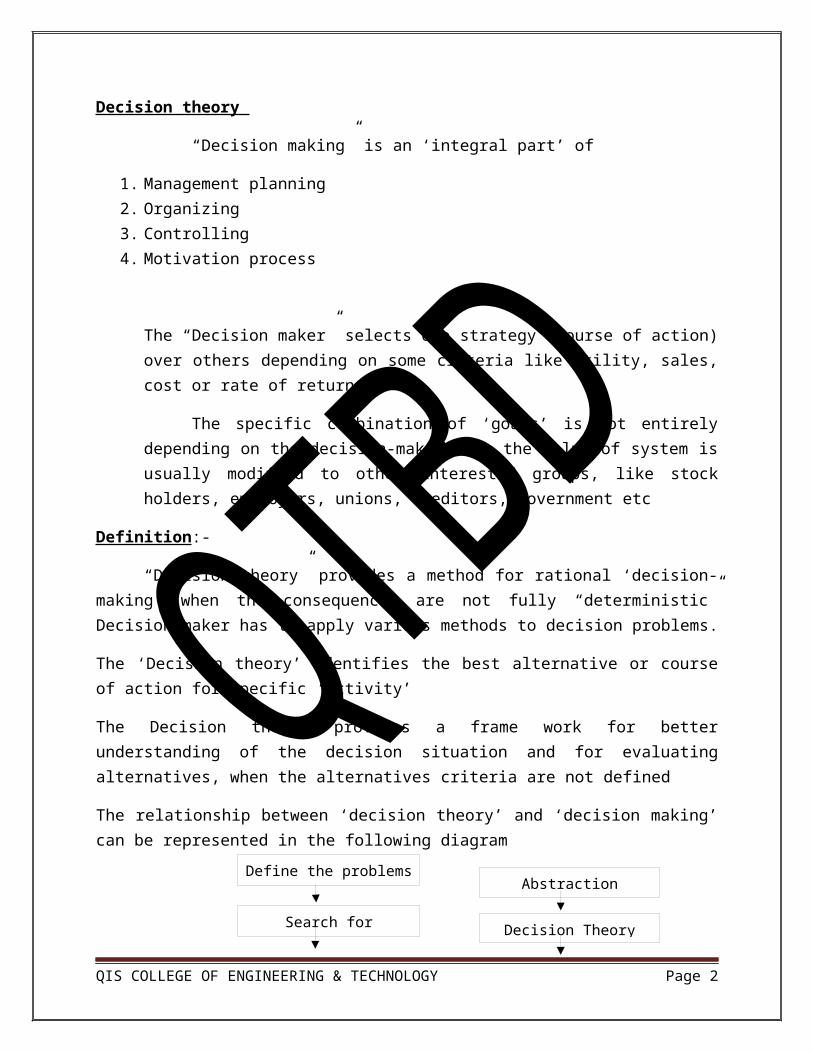
Decision theory

“Decision making” is an ‘integral part’ of

1. Management planning 2. Organizing3. Controlling 4. Motivation process

The “Decision maker” selects one strategy (course of action) over others depending on some criteria like utility, sales, cost or rate of return

The specific combination of ‘goals’ is not entirely depending on the decision-maker i.e. the value of system is usually modified to other interested groups, like stock holders, employers, unions, creditors, government etc

Definition:-

“Decision theory” provides a method for rational ‘decision- making’ when the consequences are not fully “deterministic” Decision maker has to apply various methods to decision problems.

The ‘Decision theory’ identifies the best alternative or course of action for specific ‘activity’

The Decision theory provides a frame work for better understanding of the decision situation and for evaluating alternatives, when the alternatives criteria are not defined

The relationship between ‘decision theory’ and ‘decision making’ can be represented in the following diagram

Define the

QIS COLLEGE OF ENGINEERING & TECHNOLOGYPage 2

Define the problems

Search for Alternatives

Evaluate Alternatives

Abstraction

Decision Theory

Asses Consequences

Apply Decision CriteriaSelect an Alternative

Decision:-

If a “decision” is to be made on the basis of one of the “decision criteria” then the selection of an alternative course of action is a direct effect of “decision theory” But, if alternative course of actions is compared with the considerations other than so called “pure criteria” then the “decision theory” helps us in the evaluation of alternatives.

Types of decisions:-

In general decisions can be classified into 3 categories

1. Strategic decisions2. Administrative decision 3. Operating decision

1. Strategic decisions:-

These decisions are concerned with external environment of the organization

Example:- Decision of selection of product-mix which a firm will produce and the markets to which it with sell are under strategic decisions

2. Administrative decisions:-

This is concerned with structuring and accusation of the organization resources, so as to optimize the performance of the organization

Example: - 1. Selection of distribution 2. Location of facilities

3. Operating Decision :-

This is the primary concerned with ‘day-to-day’ operations of the organization

Examples: - 1. Pricing 2.Production scheduling 3. Inventory levels etc

Components of Decision Making:-

Various components of the problem which a problem person should know are briefly discussed as follows

1. The decision maker


2. Objectives3. The system or environment 4. Alternative course of action 5. Choices

1. Decision Maker (or) Policy-Maker (or) Executive:-

Most obvious component is the fact that someone belonging ‘some group’ must have ‘some problem’ this individual or group is dissatisfied with some aspect of the state of affairs and consequently wants to make a decision with regarding to altering it, which is known as ‘decision maker’ if the ‘decision maker’ controls the operations of an organized system of men or machines then he is referred to as “policy maker” or “executive”.

2. Objectives

In order to have a problem the “decision maker” he must know something other than what he has i.e. he must have some objectives which he has not obtained to the degree he desires

3. System (or) environment:-

The ‘decision maker’ has the problem in an environment or setting that constraints or lacks various resources

“Environment” is an “organized system” usually embracing machines as well as man

4. Alternative Course of Action:-

A problem cannot exist unless the ‘decision maker’ has a choice from among at least 2 alternative courses of ‘action or policies’ A problem always involved a question what to do this question becomes a problem only when alternative courses of action are available

Decision Models

One of the primary functions of management is to make decisions that determine the future course of action for the organization involving short term or long-term consequences


Decision models are classified into various categories, depending upon their nature and complexity, such as allocation so as to optimize the given objective function subject to certain restrictions

I. Goals to be achieved :-

The objective which the decision maker wants to achieve by his action

II. The Decision-Maker :-

The decision-maker refers to an individual or a group of individuals responsible for making a choice of an appropriate course of action amongst the available course of action

III. Course of Action (or) Decision- Alternatives:-

For a specified problem all possible course of action should be included the number of possible courses of action may be large or small but these are under control of decision-maker

Example: - A course of action has a numerical description such as stocking of 150 units of a particular item or non-numerical description.

IV. States of Action :-

Before applying decision theory we must develop an exhaustive list of possible future events. Forever decision maker has no direct control over the occurrence of particular event such future events are referred to as “states of nature” and it is assumed but these are mutually exclusive collectively exhaustive

Examples:- the state of nature can be a numerical description such as demand of some units of a given item or a non- numerical description like employees strike.

V. Preference (or) Value System

This refers to the criteria that the decision maker uses in making a choice of the best course of action. It could include maximization of income utility profit etc.

VI. Pay of (or)Profit (or)Conditional Value

It is the effectiveness associated with specified with combination of a course of action and state of nature. These are also known as profit or conditional value.

Example: -The conditional profit can also be of Rs 15 associated with the action of stocking 20units of an item when the outcome is a demand of 17 units of that item. costs can be considered as negative profits.


VII. Opportunity Loss Table :-Opportunity loss is incurred due to failure of not adopting most favorable course of action or strategy the opportunity los values are determined separately for each state of nature or outcome by 1stfinding the most favorable course of action for that state for nature or outcome. And then taking the difference between pay off value for given course of action and the payoff value for the best possible course of action which would be chosen.

VIII. Pay off Table For a problem a payoff table exists the states of nature which are mutually exclusive and collectively exhaustive and as set of given courses of action (strategies). For each combination of state of nature and course of action the payoff is determined

Course of ActionStates of Nature

S1 S2 ………… S j ………… Sn

O1 a11 a12 ………… a1 j ………… a1n

O2 a21 a22 ………… a2 j ………… a2n

::

::

::

………… ::

…………

Oi a i1 a i2 ………… a ij ………… a¿

::

::

::

………… ::

………… ::

Om am1 am2 ………… amj ………… amn

The weighted profit associated with the given combination of state of nature and course of action is obtained by multiplying the payoff the state of nature and course of action by the probability of occurrence of the specified state of nature

The table shown in the above is one such type of pay off table in this table ‘m’ states of nature and denoted by O, O2 … Om with respect to ‘n’ course of action S1 S2 …. Sn for a specified combination of state of nature and course of action the corresponding payoff is represented by ai j.

Types of Environment

Decision theory helps the decision maker in selecting the best course of action from the available course of action. The decision models are classified such that the type of information which is given about the occurrence of the various state of nature as well as depending upon the decision environment basically there are 4 different states of decision environment


i. Decision making under certainty ii. Decision making under un-certainty iii. Decision making under riskiv. Decision making under conflict

I. Decision Making Under Certainty

This is all easiest form of ‘decision making’ the outcome resulting from the selecting of a particular course of action given with certainty. There is just one state of nature for each course of action and has probability ‘I’ we are given complete and accurate knowledge of the consequence of each choice. Since the decision maker has perfect knowledge of the future and the outcome, he simply selects that course of action for which the payoff is optimum

Example

The analysis of cost profit and volume is a “decision problem under certainty”

Where the information regarding costs and profits is given with respect to volume of sales. Similarly in L.P.P the amount of resources required and the corresponding unit profit (cost) is given with certainty the other techniques used for solving problems under certainty are

I. Input –output analysis II. Break- even analysis III. Goal programming IV. Transportation and assignment methods V. Inventory models

1. Decision Making Under Uncertainty :-

In the absence of knowledge about the probability of any state of nature occurring, the decision maker must arrive at a decision only on the actual conditional pay off values, together with a policy. There are several different criteria of decision- making in this situations

Types of criteria

1. Optimism criterion or maximum criterion or minimum criterion 2. Pessimism criterion or maximum criterion or minimum criterion 3. Laplace criterion or equal probabilities criterion 4. Hurwitz criterion or coefficient of optimism5. Regret criterion or salvage criterion


1. Optimism Criterion:-

In this criterion the decision-maker ensures that he should not miss the opportunity to achieve the largest possible profit (maximum) or the lowest possible cost (minimum). Thus, he selects the alternative that represents the maximum of the maximum payoff. The working method is summarized as follows.

Step-1 locate the maximum (minimum) payoff values corresponding to each alternative

Step-2 Select an alternative with best anticipated payoff value (maximum for profit) and minimum for cost)

Since in this criterion the decision-maker selects an alternative with largest (or lowest) possible payoff value, It is also called an “optimistic decision criterion”

2. Pessimism Criterion

In this criterion the decision-maker ensures that he would earn no less than some specified amount. Thus, he selects the alternative that represents the maximum of the minimum payoff in the case of profits. The working method is summarized as follows

Step-1 Locate the minimum (or maximum in the case of profit). Payoff value in the case of loss data corresponding to each alternative.

Step-2 Select an alternative with the best anticipated pay off value (maximum for profit and minimum for loss)

Since in this criterion the “decision –maker” is conservative about the future and always anticipates the “worst possible” outcome. Then it is called a “pessimistic decision criterion”. This criterion is also known as “wald’s criterion”

3. Laplace Criterion

Since the probabilities of states of nature are not known, it is assumed that all states of a nature will occur with equal probability .i.e. each state of nature is assigned an equal probability. As states of nature are mutually exclusive and collectively exhaustive, so the probability of each of these must be

1(number of states of nature)

the working method is summarized as follows.

Step-1 Assign equal probability value to each state of nature by using formula

1(number of states of nature)


Step -2 Compute the expected (average) pay off for each alternative by adding all the payoffs and dividing by the number of possible states of nature by applying the formula ⟹ ( Probability of state of nature ) X

(Payoff value for the combinations of alternative ‘i’ and state of nature ‘j’)

Step-3 Select the best expected pay off value (maximum for profit and minimum for cost)

This criterion is also known as the criterion of “insufficient reason” this is because except in a few cases, some information of the likelihood of occurrence of states of nature is available

4. Hurwitz Criterion:

This criterion suggest that a rational decision- maker should be neither completely optimistic nor pessimistic and must display a mixture of both Hurwitz also suggested this criterion, introduced the idea of a coefficient of optimism which is denoted to measure the decision maker’s degree of optimism. This coefficient lies between o & 1.

Where 0= A complete pessimistic attitude about the future

1= A complete optimistic attitude about the future

α = Coefficient of optimism attitude about the future

(1- α )= Coefficient of pessimism

The Hurwitz approach suggests that the decision-maker must select alternative that maximizes

H (Criterion of realism) = (maximum in column) + (1- α )(minimum in column the working method is summarized as follows.

Step-1 Decide the coefficient of optimism. And the coefficient of pessimism (1-α )

Step-2 For each alternative select the largest and lowest pay off value and multiply these with and (1-α ) values respectively. Then calculate the weighted average H by using above formula

Step-3 Select the course of action with the smallest anticipated opportunity loss value

Step-3 Select an alternative with best anticipated weighted average payoff value.

5. Regret Criterion


This criterion is also known as opportunity loss decision” criterion or “Minimax Regret decision” criterion. This is because decision- making regrets the fact that he adopted a wrong course of action resulting in an opportunity loss of payoff. Thus, he always intends to minimize this regret the working method is summarized as follows

Step-1 From the given payoff matrix, develop an opportunity loss matrix as follows

1. Find the best pay off corresponding to each sate of nature 2. Subtract all other entries in that row form this value

Step-2 For each course of action identify the worst or maximum regret value record this number in a new row

Step -3 Select the course of action with the smallest anticipated opportunity loss value

Problems on – Decision Making Under Uncertainty

Problem -1

A food products company is contemplating the introducing of a revolutionary new product with new packaging or replacing the existing product at much higher price (s1). It may even make a moderate change in the composition of the existing product, with a new packaging at a small increase in price (s2) or may be a small change in the composition of the existing product, backing it with the word “new” and a negligible increase in price (S3) the 3 possible states of nature or events are high increase in sales (N1), No change in sales (N2), Decrease in sales (N3)

The marketing department of the company worked out of payoffs in terms of yearly net profits for each of the strategies of ‘3’ events this is presented in the following table

States of nature strategies

N1 N2 N3

S1

S2

S3

7,00,000

5,00,000

3,00,000

3,00,000

4,50,000

3,00,000

1,50,000

0

3,00,000


Which strategy should the concerned executive choose on the basis of

I. Maximum criterion II. Maximax criterion III. Minimax criterion IV. Laplace criterion

Solution

The payoff matrix is rewritten as follows

a) Maximin criterion or (pessimistic criterion)

States of nature strategies

S1 S2 S3

N1

N2

N3

7,00,000

3,00,000

1,50,000

5,00,000

4,50,000

0

3,00,000

3,00,000

3,00,000

Column Minimum1,50,000 0 3,00,00

0

The maximum of column minima is 3,00,000. Hence, the company should adopt strategy S3

b) Maximax criterion or (optimistic criterion)

States of nature Strategies

S1 S2 S3


N

N

N

7,00,000

3,00,000

1,50,000

5,00,000

4,50,000

0

3,00,000

3,00,000

3,00,000

Column maximum 7,00,000 5,00,000 3,00,000

The maximum of column maxima is 7, 00,000. Hence the company should adopt strategy S1

C) Minimax Regret Criterion or (Regret Criterion :

States of nature

Strategies

S1 S2 S3

N1 7,00,000-7,00,000=0 7,00,000-5,00,000= 2,00,000 7,00,000-3,00,000=4,00,000

N2 4,50,000-3,00,000=1,50,000

4,50,000-4,50,000=0 4,50,000-3,00,000=1,50,000

N3 3,00,000-1,50,000=1,50,000

3,00,000-0=3,00,000 3,00,000-3,00,000=4,00,000

Column maximum

1,50,000 3,00,000 4,00,000

Hence the company should adopt minimum opportunity loss strategy of ‘S1’

D) Laplace Criterion or (Equal Probability Criterion):


Since we do not know the probabilities of states of nature, assume that they are equal. For example we should assume that state of nature has probability 13

of occurrence. Thus

Strategy Expected return (Rs)

S1 (7,00,000+3,00,000+1,50,000)/3 = 3,83,333.33

S2 (5,00,000+4,50,000+0)/3 = 3,16,666.66

S3 (3,00,000+3,00,000+3,00,000)/3 = 3,00,000

Since the largest expected return is from strategy S1 then the executive most select strategy S1

Solution:-

1. Maximin criterion is strategy S3 ( pessimistic criterion)2. Maximax criterion is strategy S1 ( optimistic criterion )3. Minimax criterion is strategy S1 (regret criterion)4. Laplace criterion is strategy S1 ( equal probability criterion)

Problem-2

A manufacturer manufactures a product, of which the principal ingredient is a chemical ‘X’. At the moment the manufacturer spends Rs 1,000/- per year on supply of ‘X’ but there is a possibility that the price may soon increase to ‘4’ time it’s another chemical ‘Y’ which the manufacturer could use in conjunction with a 3rd chemical Z, in order to give the same effect as chemical ‘X’ chemicals Y and Z would together cost the manufacturer Rs 3,000 for year, but their prices are unlikely to rise. What action should the manufacturer taken? Apply the maximin and minimax criteria for decision- making and give ‘2’ sets of solution. If the coefficient of optimism is 0.4, then find the course of action that minimizes the cost

Solution :-

The data of the problem is summarized in the following table


States of nature Courses of action

S1 ( use Y and Z) S2 ( use X)

N1 ( price of X increases) -3,000 -4,000

N2 ( price of X does not increase )

-3,000 -1,000

1. Maximin Criterion or ( Pessimistic Criterion):


S1 S2

N1

N2

-3,000

-3,000

-4,000

-1,000

Column minimum -3,000 -4,000

The maximum of column minimum is -3,000. Hence the manufacture should adopt the action ‘S1’

2. Minmax Criterion or ( Pessimistic Criterion )

States of nature Course of action

S1 S2

N1

N2

-3,000-(-3,000)=0

-1,000-(-3,000)= 2,000

-3,000-(-4,000) =1,000

-1,000-(-1,000)=0

Maximum opportunity 2,000 1,000

Hence, manufacturer should adopt minimum opportunity less course of action

3. Hurnicz criterion or ( Coefficient of Optimistic)

Given that coefficient of optimism = = 0.4

Coefficient of pessimism = (1- α) = 1-0.4=0.6


Then according to Hurwitz, select course of action that optimizes (maximum for profit and minimum for loss) the payoff value.

H= (best pay off) + (1- α ) (Worst payoff)

= (maximum in column) + (1- α ) (minimum in column)


S1 S2

N1 -3,000 -4,000

N 2 -3,000 -1,000

Column maximum -3,000 -1,000

Column minimum -3,000 -4,000

Course of action Best payoff Worst pay off H= 0.4 (best payoff) +0.6 (worst payoff)

S1 -3,000 -3,000 = 0.4 (-3,000) +0.6 (-3,000) = (1200) –(1800)= - (3,000)

S2 -1,000 -4,000 = 0.4 (-1000) +0.6 (-4,000) = - 400- 2400= - (2800)

Since course of action S2 has the least cost (maximum profit) = Rs 2,800. The manufacturer should adopt strategy ‘S2’

I. Decision Making – Under Certainty Decision Tree Analysis Problems

Problem-1

You are given the following estimates concerning a and development programmer

Decision Di

Probability of decision (Di) given (R) P

Outcome Probability of given research

Pay off value of outcome Xi


(Di/R)(R) P(Xi/Di) (Rs’ 000)

Develop 0.5

1 0.6 600

2 0.3 -100

3 0.1 0

Do not develop 0.5

1 0.0 600

2 0.0 -100

3 1.0 0


P(x3/D2)

Construct and evaluate the decision tree diagram for the above data. Show working for evaluation

Solution The “decision tree” of the given problem along with necessary calculations is shown in the following diagram


2

3

4

5

6

7

8

D1

Develo

Do not develop

D2

=0.6

P(x2/di)

0.3

D(x3/Di)

=0.1

P(xi/D2)

=0

D(x2/D2)

=0

P (xi/di)

1

=1.0

Probability Pay off in (Rs’ 000) Expected pay off (in Rs’ 000)

0.5 x 0.6 =0.3

0.5 x 0.3= 0.15

0.5 x0.1= 0.05

600

-100

0

=0.3 x 600= 180

=0.15 x -100=-15

=0.05 x 0=0

Total 165

0.5 x 0= 0

0.5 x 0 = 0

0.5 x 1.0= 0.05

600

-100

0

=0 x 600 =0

= 0 x (-100) =0

=(0.05) x 0 = 0

Total 0

Problem -2

A businessman has 2 independent investment portfolios A and B available to him, but he lacks the capital to undertake both of them simultaneously. He can either choose a first and then stop, or if A is not successful, then take. B or vice versa the probability of success of A is 0.6 white for B it is 0.4. Both investment schemes require are initial capital outlay of Rs 10,000 and both return nothing if the venture process to unsuccessful. Successful completion of A will return Rs 20,000 and Successful completion of B will return Rs 24,000 Draw a decision tree in order to determine the best strategy.

Solution: - The decision tree corresponding to the given information is as followed


DECISION POINT OUT COME PROBABILITY CONDITIONAL VALUE (RS/-)

EXCEPTED VALUE

D3

1.ACCPT A

SUCCESS/

FAILURE

0.6

0.4

23,000/-

-10,000/-

12,000/-

-4,000

8,000

2.STOP 0

D2

1.ACCEPT B

SUCCESS/

FAILURE

0.4

0.6

24,000/-

-10,000/-

9,600/-

-6,000/-

3,6000/-

2.STOP 0

D1

1.ACCPT A

SUCCESS/

FAILURE

0.6

0.4

20,000+3,600 =23600 × (0.6)

-10,000×(0.4)

14,160

-4,000

10,160

2.ACCEPT B SUCCESS/

FAILURE

0.4

0.6

24000+8000=

32000 ×(0.4)

-10,000×(0.6)

12800

-6,000

6,800


(0.6) EMV=3600 SUCCESS

EMV =10,160 0.6 FAILURE

RS/10,000

EMV=6,800 RS/-24000 ACCEPT A

SUCCESS

RS/-0

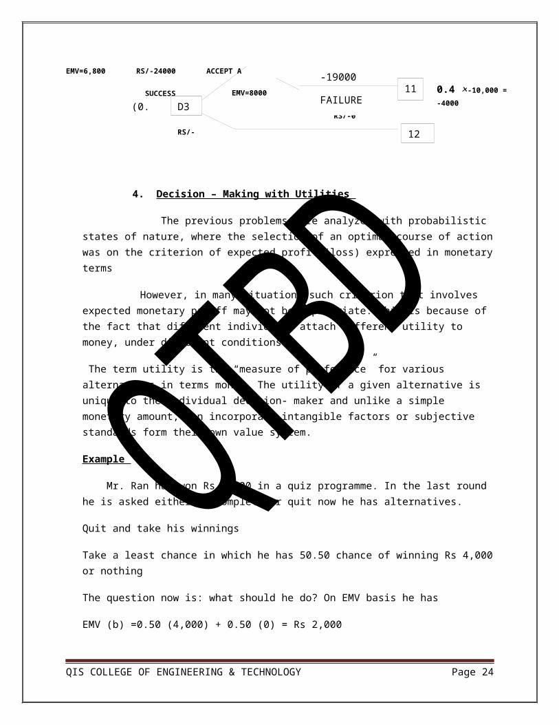
4. Decision – Making with Utilities

The previous problems were analyzed with probabilistic states of nature, where the selection of an optimal course of action was on the criterion of expected profit (loss) expressed in monetary terms

However, in many situations such criterion that involves expected monetary payoff may not be appropriate. This is because of the fact that different individuals attach different utility to money, under different conditions.


D1

1

D2

3

4

8

9

5

2

D3

6

7

10

11

12

ACCEPT A

SUCCE

SS

Rs/- 3600

0.4

STOP

RS/- 0

RS/-20,000

ACCEPT B

FAILURE

RS/-10,000

0.4×24,000=9600

0.6 ×-10,000 =-6,000

ACCEPT BFAILURE

(0.4)

RS/-8000

EMV=8000

SUCCESS (0.6)

FAILURE (0.4)

RS/-20000

-19000

0.6 × 20,000 =12,000

0.4 ×-10,000 = -4000

The term utility is the “measure of preference” for various alternatives in terms money. The utility of a given alternative is unique to the individual decision- maker and unlike a simple monetary amount, can incorporate intangible factors or subjective standards form their own value system.

Example

Mr. Ran has won Rs 1,000 in a quiz programme. In the last round he is asked either to complete or quit now he has alternatives.

Quit and take his winnings

Take a least chance in which he has 50.50 chance of winning Rs 4,000 or nothing

The question now is: what should he do? On EMV basis he has

EMV (b) =0.50 (4,000) + 0.50 (0) = Rs 2,000

The amount is twice what he was already won. But would he really give up Rs 1,000 for 50-50 chance or Rs 4,000 or nothing? Many individuals would not because they would think of all the alternatives they could do with Rs 1,000 and how they would regret it if they end up with nothing hence a new payoff measure utility reflecting the decision- makers attitude and preference has to be introduced.

The basis axioms of utility may be stated as follows.

1. If outcome A is proffered to outcome B, they the utility U(A) of outcome A is greater than the utility u(B) of outcome B vice versa

If both are equally proffered then u(A) = u(B)2. If the decision-maker is different between the ‘2’ alternatives and outcome

‘A’ is received with probability P1 and outcome C with probability (1-P) then U (B) = P [U (A)] + (1-P) [U/C)]

Under this alternative criterion, it is assumed that a rational decision-maker will choose that alternative which optimize the “expected utility” rather than expected monetary value. Once we know that individual’s utility function, along with the probability assigned to outcome in a particular situation then the total expected utility for each course of action can be obtained by multiplying the utility values with their probabilities the strategy that corresponds to the optimum utility function is called that equal strategy”

Utility function


“Utility function” is a formula or method that is used to describe the relative preference value that individuals have for a given criterion such as money, goods etc.

Once derive, a “utility function” can be used to convert a decision criteria value into utilities so that a decision can be made on the bass of maximizing the expected “utility value” (EUV) rather than, say the “EMV”

Example

Preference are often determined by proposing a situation where by decision- maker must choose between receiving a given amount, say Rs 20,000 for a certain thing versus a 50-50 chance of gambling a larger amount or nothing say Rs 60,000 or Zero. The gamble amount of Rs 60,000 is then adjusted upward or down ward until the individual is indifferent to whether decision – maker receives the certain amount of Rs 20,000 or the gamble

Utility Curve

A utility curve that relates utility values to rupee value is construction such a curve is usually obtained by placing the decision maker in various hypothetical decision situations and plotting the decision makers pattern of choices in terms of risk and utilities.

Suppose the relationship between monetary gains, losses and utilities for gains and for small negative losses is established. The following diagram shows that if the curve is bent down non- linearly then we assign, to large losses a disproportionately large negative utility. It is important not to make the curve bend down too steeply or to start the bending too quickly since this could lead individuals into a situation where they attach such a heavy to the possibility of loss they never take any risk and tell us never masse any gains

Once the +ve side of the curve, it is usual for the curve to eventually bend away from the straight line. This indicates that increasing units of money are resulting in smaller additional gains in utility

U MAX

RISK AVERSION (AVOIDERS)

UTILITY RISK INDIFFERENCE (NEUTRALITY)


RISK AFFINITY (SEEKERS)

Problem 1

A manager must choose between 2 investments A&B that are calculated to yield net profit of Rs 1,200 and Rs 1,600 respectively. With probabilities subjectively estimated at 0.75 and 0.60. Assume the manager’s utility function reveals that utilities for Rs 1,200 and Rs 1,600 are 45 and 50 units respectively what is the best choice on the basis of the expected utility value (EUV)?

Solution

The except utility value (EUV) is expressed as

EUV = ∑i=1

m

u i pi where ui= utility value of state of nature i

pi = probability value of state of nature iEUV (A) = (U A ¿ (pA) = (0.75) (45) =33.75 = EUV (A) =33.75 utilities EUV (B) = (U B¿ (pB) = (0.60) (50) =30.00 = EUV (B) =30 utilities ⟹ 30< 33.75

Since EUV (A) > EUV (B)

The best choice is investment “A”

Problem 2

Mr. X has an after –tax annual of Rs 90,000 and is considering to buy accident insurance for his car. The probability of accident during the year is 0% (Assume that at most one accident will occur) in which case the damage to the car will be Rs 11,600 which a utility function U(x)=√ x, what is the insurance premium he will be willing to pay?

Solution: Let A = Venture when Mr. X does not buy the accident insurance for his car. Then in that case of accident he would spend Rs. 11,600 on damages and


MONEY RS/- MAX

will be left with Rs. 78,400. In the case for no accident he retains Rs. 90,000. Then we have

U A = (U 78,400 X 0.1) + (U 90,000 X 0.9) →1

U (x) = U X = √X →2

U 78,400 = √78,400 = 280 utilities→3 U 90,000 = √90,000 = 300 utilities

→4

U A = (280 X 0.1) + (300 X 0.9) = 298 utilities →5

So the amount Rs. X which will give the same utility of the venture

A = (298)2 = Rs. 88,804 [∵ U (x) = √X ⟹X = [ U (x )¿¿2 ]

Thus Mr. X will be indifferent to an amount of Rs.88, 804 with certainty and the venture A. The amount he is willing to pay as car premium would be

90,000 – 88,804 = Rs. 1,196

3) Decision Making Under Risk:

Decision making under risk is a probabilistic decision situation in which more than one state of nature exists. And the decision maker has sufficient information to assign probability values to the likely occurrence of each of these states. Knowing the probability distribution of these states of nature, the best decision is to select that course of action which has the largest expected payoff value.

The expected (average) payoff of an alternative is the sum of all possible payoffs of that alternative, weight by the probabilities of the occurrence of those payoffs.

The most widely used criterion for evaluating various course of action (alternatives) under risk is the “expected monetary value (EMV)” or “expected utility”

Expected Monetary Value (EMV)

The expected monetary value (EMV) for a given course of action is the weighted sum of possible payoffs for each alternative. The expected value is the long-run average value that would result if the decision were repeated a large number of times. Mathematically EMV is stated as follows.

EMV [ Course of avtion, Sj ] = ∑i−1

n

pij .Pi


Where m = number of possible states of nature

Pi = probability of occurrence of nature, N:

Pij= payoff associated with state of nature Ni and course of action, Sj

Steps for calculating EMV

The various steps involved in the calculation of EMV are as follows

1. Construct of payoff matrix listing all possible courses of action and states of nature. Enter the conditional payoff values associated with each possible combination of courses of action and state of nature along with the probabilities of the occurrence of each state of nature

2. Calculate the EMV for each course of action by multiplying the conditional payoff by the associated probabilities and adding these weighted values for each of action

3. Select the course of action that yields the optimal EMV

Expected Profit with Perfect Information (EPPI )

The expected profit with perfect information (EPPI) is the maximum attainable expected money value (EMV) based on perfect information about the state of nature that will occur. The expected profit with perfect information may be defined as the sum of the product of best state of nature corresponding to each optimal course of action and its probability

Expected Value of PerfectInformation ( EVPI)

The expected value of perfect information (EVPI) may now be defined as the maximum amount one would be willing to pay to obtain perfect information about the state of nature that would be willing to pay to obtain perfect information about the state of nature that would occur. EMV Represents the maximum attainable expected monetary value given only the prior outcome probabilities with no information as to which state of nature will actually occur. Therefore perfect information would increase profit from EMV up to the value of EPPI. This increased amount is termed as EVPI.

i.e. EVPI= EPP1- EMV

Expected Opportunity Loss ( EOL):

Another useful way of maximizing monetary value is to minimize the expected loss or expected value of regret. The conditional opportunity los (COL) or regret


function for a particular course of action is determined by taking the difference between payoff values of the most favorable course of action. And some other course of action .Which may be considered as loss due to loosing the opportunity of choosing the most favorable course of action, thus opportunity loss can be obtained separately for each course of action by 1St obtaining the best state of nature for the prescribed course of action and then taking the difference between that best outcome and each outcome for those courses of action. The opportunity loss for each course of action is known as the conditional opportunity loss

After calculating the opportunity loss value for each course of action,

the E0L for ith course of action Si is then computed by

EOL (Si,) =∑j=1

n

COL¿¿ Si,O j). P (O j)

Where (Si,O j)= Conditional Opportunity loss associated with the course of action Si

And state of nature O j.

P (O j ) = Probability of occurrence of state of natureO j.

In other words EOL denotes the expected difference between the payoff of right

decision and the payoff of actual decision.

Problem-1

A modern home appliances dealer finds that the cost of holding a mini cooking

range is stock for a month is Rs 200 (Insurance, minor deterioration, interest on

borrowed capital, etc) customer who cannot obtain a working range immediately

tends to go to other dealer and he estimates that for every customer who cannot

get immediate delivery, he loses an average of Rs 500 the probabilities of a demand

of 0,1,2,3,4,5 mini cooking ranges in a month are 0.05, 0.10, 0.20, 0.30, 0.20, 0.15


respectively determine the optimum stock level of consuming rangers. Also find

EVPI

Solution:

The cost function =Rs 500(D-S); If D>S = Rs 200 (S-D); If D < S

Where S= The number of units purchased and D= the number of units

demanded.

Event

Demanded

(D)

Probabili

ty

Conditional Cost (Rs/-) (S) Expected Cost (Rs/-)

0 1 2 3 4 5 0 1 2 3 4 5

0 0.05 0 200 400 600 80

0

100

0

0 10 20 30 40 50

1 0.10 500 0 200 400 60

0

800 5

0

0 20 40 60 80

2 0.20 100

0

500 0 200 40

0

600 200 100 0 40 80 12

0

3 0.30 150 100 500 0 20 400 450 300 20 10 0 40


0 0 0 0 0

4 0.20 200

0

150

0

100

0

500 0 200 400 300 20

0

10

0

0 40

5 0.15 250

0

200

0

150

0

100

0

50

0

0 375 300 22

5

15

0

7 50

Expected cost 147

5

101

0

61

5

36

0

31

5

41

0

Since the expected cost is minimum if 4 cooking ranges are stocked each month.

The optimum act is to stock 4 looking ranges.

Problem -2

Under an employment promotion programming, it is proposed to allow sale of

newspapers on the buses during of peak hours. The vendor can purchase the

newspaper at a special concessional rate of 25 paisa per copy against the selling

price of 40 paise. Unsold copies are however a dead loss. A vendor has estimated

the following probability distribution for the number of copies demanded

No of copies demanded 15 16 17 18 19 20

Probability 0.04 0.19 0.33 0.26 0.11 0.07

How many copies should he order so that his expected profit will be maximum?

Solution:-


The vendor does not purchase less than 15 copies or more than 20 copies

Let n = The number of copies of newspaper demanded

The vendor would loss 25 paise on each copy in case of demand is less than ‘n’

otherwise , if the demand is more than or equal to ‘n’ then he would gain 15 paise

on each newspaper copy .

The incremental profit =( Excepted profit –Expected loss), for each value on ‘n’

is given in the following table

Expected profit

Demand (n) Probability(<n)

Probability(>n)

Expected incremental Profit (Rs-/)

Total profit

15 0.00 1.00 =0(0)+1(0.15)=0.15

0.15×15=2.25

16 0.04 0.96 =0.04(-0.25)+0.96(0.15)=0.13

0.13×16=2.38

17 0.23 0.77 =0.23(-0.25)+0.77(0.15)=0.06

0.06×17=2.44

18 0.56 0.44 =0.56(-0.25)+0.44(0.15)=(-0.07)

0.07×18=2.37

19 0.82 0.18 =0.82(-0.25)+0.07(0.15)=

0.18×19=2.19


(-0.18)

20 0.93 0.07 =0.93(-0.25)+0.07(0.15)=(-0.22)

00.22×20 =1.97


Education

decision tree in quantitative analysis