Factorization from Gaussian Elimination

분산시스템 연구실

6. LU Factorization

12-cs-029 Mudassir Ali


Contents

• LU Factorization from Gaussian Elimination

• LU Factorization of Tridiagonal Matrices

• LU Factorization with Pivoting• Direct LU Factorization• Application of LU Factorization• Matlab’s Method


Example. Circuit Analysis Application

Solve by LU Factorization of coeff icient matrix

0V1 =

0V2 =

200V3 =

20R1 = 25R 3 =

30R 5 =10R 2 =

10R 4 =1i

2i

3i

200)(10)(1030

0)(20)(1025

0)(10)(20

13233

12322

3121

=-+-+

=-+-+

=-+-

iiiii

Flow around lower loop

iiiii

Flow around upper loop

iiiiFlow around the left loop


6.1 LU Factorization from Gaussian Elimination


LU Factorization from Gaussian Elimination

- Example 6.1

=

28143

1062

321

A

Example 6.1 Three-By-Three System

=

100

010

001

L, ,

=

28143

1062

321

U

Step 1:

=

103

012

001

L ,

=

1980

420

321

U

Step 2:

=

103

012

001

L ,

=

1980

420

321

U

Multiply L by U, and Verify the result:

LU =

103

012

001

1980

420

321. =

28143

1062

321

= A

=

28143

1062

321

A ,

=

28143

1062

321

A ,



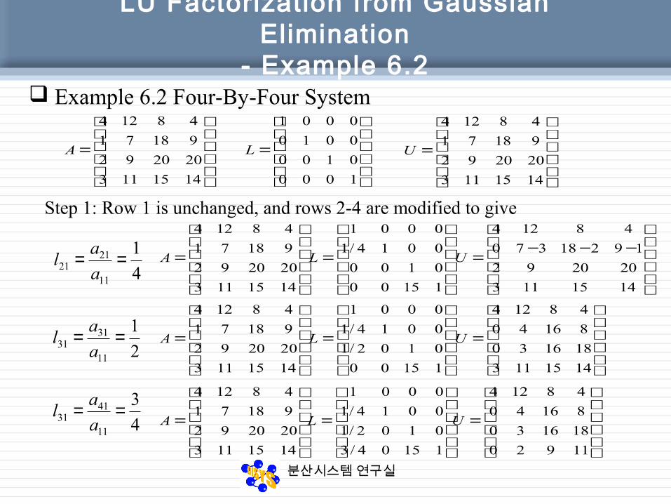
- Example 6.2 Example 6.2 Four-By-Four System

=

1415113

202092

91871

48124

A

Step 1: Row 1 is unchanged, and rows 2-4 are modified to give

4

1

11

2121 ==

a

al

2

1

11

3131 ==

a

al

4

3

11

4131 ==

a

al

=

11920

181630

81640

48124

U

=

1000

0100

0010

0001

L

=

1415113

202092

91871

48124

U

=

1415113

202092

91871

48124

A

=

11500

0100

0014/1

0001

L

−−−

=

1415113

202092

19218370

48124

U

=

1415113

202092

91871

48124

A

=

11500

0102/1

0014/1

0001

L

=

1415113

181630

81640

48124

U

=

1415113

202092

91871

48124

A

=

11504/3

0102/1

0014/1

0001

L



- Example 6.2

Step 2: Row 1 and 2 are unchanged, row 3 and 4 are transformed, yielding

Example 6.2 Four-By-Four System

4

3

22

3232 ==

a

al

2

1

22

4242 ==

a

al

=

7100

12400

81640

48124

U

Step 3: The fourth row is modified to complete the forward elimination stage:

4

1

33

4343 ==

a

al

=

4000

12400

81640

48124

U

=

102/14/3

014/32/1

0014/1

0001

L

=

1415113

202092

91871

48124

A

=

14/12/14/3

014/32/1

0014/1

0001

L

=

1415113

202092

91871

48124

A



- Example 6.2

Multiply L by U to verify the result:

Example 6.2 Four-By-Four System

14

1

2

1

4

3

014

3

2

1

0014

10001

4000

12400

81640

48124

.

1415113

202092

91871

48124

=

L . U = A



- MATLAB Function for LU Factorization 6.1.1 MATLAB Function for LU Factorization Using Gaussian Elimination

function [L, U] = LU_Factor(A)% LU factorization of matrix A% using Gaussian elimination without pivoting% Input : A n-by-n matrix% Output L ( lower triangular ) and% U (upper triangular )[n, m] = size(A);L = eye(n); % initialize matricesU = A;for j = 1 : n

for I = j + 1 : nL( i , j ) = U( i, j ) / U( j, j );U( i , : ) = U( i, j ) / L( j, j ) * U( j, : );

endend% display L and ULU% verify resultsB = L * UA



- MATLAB Function for LU Factorization>> LU_factor(A);

L =

1.0000 0 0 0 0.2500 1.0000 0 0 0 0 1.0000 0 0 0 0 1.0000L =

1.0000 0 0 0 0.2500 1.0000 0 0 0.5000 0 1.0000 0 0 0 0 1.0000L =

1.0000 0 0 0 0.2500 1.0000 0 0 0.5000 0 1.0000 0 0.7500 0 0 1.0000L =

1.0000 0 0 0 0.2500 1.0000 0 0 0.5000 0.7500 1.0000 0 0.7500 0 0 1.0000L =

1.0000 0 0 0 0.2500 1.0000 0 0 0.5000 0.7500 1.0000 0 0.7500 0.5000 0 1.0000

L =

1.0000 0 0 0 0.2500 1.0000 0 0 0.5000 0.7500 1.0000 0 0.7500 0.5000 0.2500 1.0000L =

1.0000 0 0 0 0.2500 1.0000 0 0 0.5000 0.7500 1.0000 0 0.7500 0.5000 0.2500 1.0000U =

4 12 8 4 0 4 16 8 0 0 4 12 0 0 0 4B =

4 12 8 4 1 7 18 9 2 9 20 20 3 11 15 14A =

4 12 8 4 1 7 18 9 2 9 20 20 3 11 15 14



- Example 6.3 Example 6.3 LU Factorization for Circuit Analysis Example

1321 102030 Viii =−−

2321 105520 Viii =−+−

3321 551010 Viii =+−−

−−−−−−

=501010

105520

102030

A

Step 1: The matrices after the first stage of Gaussian elimination are

−−=

103/1

013/2

001

L

−−−−

=3/1403/500

3/503/1250

102030

U,

Step 2: The matrices after the second stage of Gaussian elimination are

−−−=

15/23/1

013/2

001

L

−−−

=4000

3/503/1250

102030

U,



- Discussion 6.1.2 Discussion

100

01

001

c .

333231

232221

131211

aaa

aaa

aaa

=

333231

232221

131211

aaa

ddd

aaa

Here, d12 = ca11+a21, d22=ca12+a22, and d32 = ca13+a32. We write this as CA = D

We also need the inverse of the matrix C

−

100

01

001

c .

100

01

001

c =

100

010

001

, or

C-1 . C = I .



- Discussion

−−

10

01

001

32

21

m

m .

10

01

001

31

21

m

m =

100

010

001

M1-1 . M1 = I .

− 10

010

001

32m

.

10

010

001

32m=

100

010

001

M2-1 . M2 = I .

−−

10

01

001

32

21

m

m

− 10

010

001

32m

. =

−−−

1

01

001

3232

21

mm

m

M1-1 . M2

-1 = I .


6.2 LU Factorization of Tridiagonal Matrix


LU Factorization of Tridiagonal Matrix

• 6.2.1 Matlab function for LU Factorization of a Tridiagonal Matrix

LU Factorization of a tr idiagonal matrix T• less computation• less computer memory


LU Factorization of Tridiagonal Matrix

function [dd, bb] = LU_tridiag(a, d, b)% LU factorization of a tridiagonal matrix T% Input% a vector of elements above main diagonal, a(n) = 0% d diagonal of matrix T% b vector of elements below main diagonal, b(1) = 0% The factorization of T consists of% Lower bidiagonal matrix,% 1’s on main diagonal; lower diagonal is bb% Upper bidiagonal matrix,% main diagonal is dd; upper diagonal is aN = length(d)bb(1) = 0;dd(1) = d(1);for i = 2 : n

bb(i) = b(i) / dd(i-1);dd(i) = d(i) – bb(i) * a(i-1);

end


LU Factorization of Tridiagonal MatrixExample 6.4

Consider again the four-by-four tridigonal matrix from Example 3.7,

−−−

−−−

=

2100

1210

0121

0012

M

four-by-four tridigonal matrix

=

44

333

222

11

00

0

0

00

db

adb

adb

ad

T

Example 6.4 LU Factorization of Tridigonal System

=

2

2

2

2

d

−−−

=

0

1

1

1

a

−−−

=

1

1

1

0

b, , ,

−−−

−−−

=

2100

1210

0121

0012

M

=

100

010

001

0001

4

3

2

bb

bb

bbL

=

4

33

22

11

000

00

00

00

dd

add

add

add

U



1) For i = 2, dd1 = d1 = 2, a1 = -1 bb2 = b2/dd1 = -1/2 dd2 = d2 – bb2a1 = 2-(-1/2)(-1) = 3/2

−

=

100

010

0012/1

0001

4

3

bb

bbL

−

=

4

33

2

000

00

02/30

0012

dd

add

aU

2) For i = 3, a2 = -1 bb3 = b3/dd2 = -1/(3/2) = -2/3 dd3 = d3 - bb3a2 = 2-(-2/3)(-1) = 4/3

−−

=

100

013/20

0012/1

0001

4bb

L

−

−

=

4

3

000

3/400

012/30

0012

dd

aU



3) For i = 4, a3 = -1 bb4 = b4/dd2 = -1/(4/3) = -3/4 dd4 = d4 - bb4a3 = 2-(-3/4)(-1) = 5/4

−−

−=

14/300

013/20

0012/1

0001

L

−−

−

=

4/5000

13/400

012/30

0012

U


6.3 LU Factorization with pivoting


6.3.1 Why pivoting?

=

−⋅

⋅=⋅

−=

=

=

331

28143

1062

200

1350

1062

102/1

012/3

001

????

1350

200

1062

...

102/3

012/1

001

28143

331

1062

APUL

UL

A


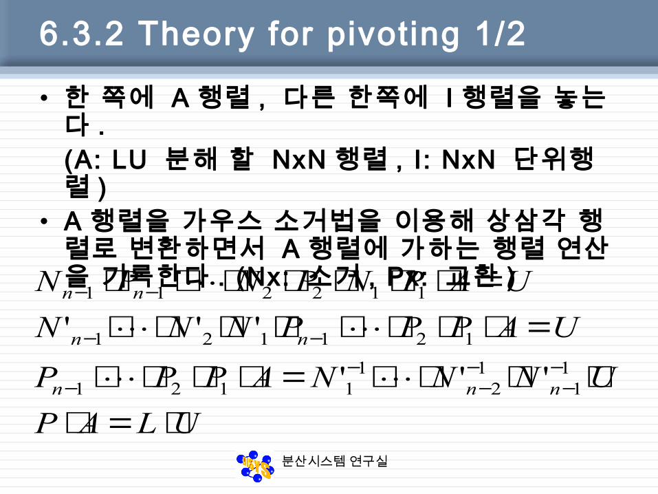
6.3.2 Theory for pivoting 1/2

• 한 쪽에 A 행렬 , 다른 한쪽에 I 행렬을 놓는다 .(A: LU 분해 할 NxN 행렬 , I: NxN 단위행렬 )

• A 행렬을 가우스 소거법을 이용해 상삼각 행렬로 변환하면서 A 행렬에 가하는 행렬 연산을 기록한다 . (Nx: 소거 , Px: 교환 )

ULAP

UNNNAPPP

UAPPPNNN

UAPNPNPN

nnn

nn

nn

⋅=⋅⋅⋅⋅⋅=⋅⋅⋅⋅

=⋅⋅⋅⋅⋅⋅⋅⋅=⋅⋅⋅⋅⋅⋅⋅

−−

−−

−−

−−

−−

11

12

11121

121121

112211

'''

'''


6.3.2 Theory for pivoting 2/2

• Nx 행렬을 좌측으로 빼면서 N’x 로 변환한다 .

• 좌측 N’x들의 역행렬을 I 행렬에 곱한다 .

=

−−−

•

−−−

=

−−−

•

−

1002

0103

0014

0001

1002

0103

0014

0001

0010

0100

1000

0001

1002

0103

0014

0001

1004

0103

0012

0001

0010

0100

1000

0001

1


6.3.3 pivoting example 1/2

=

⋅

⋅

−−⋅

=

⋅

⋅

−−

=

⋅

=

220

040

888

888

442

484

001

010

100

102/1

014/1

001

010

100

001

040

220

888

888

442

484

001

010

100

102/1

014/1

001

484

442

888

888

442

484

001

010

100

888

442

484

888

442

484


6.3.3 pivoting example 2/2

⋅

=

⋅

⋅

⋅

=

⋅

⋅

=

⋅

⋅

⋅

−−⋅

−

=

⋅

⋅

−−⋅

⋅

−

200

040

888

12/12/1

014/1

001

888

442

484

010

001

100

200

040

888

12/10

010

001

102/1

014/1

001

888

442

484

001

010

100

010

100

001

200

040

888

888

442

484

001

010

100

010

100

001

102/1

014/1

001

12/10

010

001

200

040

888

888

442

484

001

010

100

104/1

012/1

001

010

100

001

12/10

010

001


6.3.4 pivoting procedure

0010

0100

0001

1000

2220

3100

0040

8888

1008/1

0102/1

0014/1

0001

0001

0100

0010

1000

0040

3100

2220

8888

1002/1

0108/1

0014/1

0001

0001

0100

0010

1000

4484

4211

4442

8888

1000

0100

0010

0001

1000

0100

0010

0001

8888

4211

4442

4484

1000

0100

0010

0001

0100

0010

0001

1000

2000

2200

0040

8888

12/102/1

012/18/1

0014/1

0001

0100

0010

0001

1000

3100

2200

0040

8888

1002/1

012/18/1

0014/1

0001

0010

0100

0001

1000

2200

3100

0040

8888

102/18/1

0102/1

0014/1

0001


6.3.5 pivoting codeFunction [L, U, P] = LU_pivot(A)[n, n1] = size(A);L=eye(n); P=eye(n); U=A;For j = 1:n [pivot m] = max(abs(U(j:n, j))); m = m+j-1; i f m ~= j % interchange rows m and j in U % interchange rows m and j in P i f j >= 2 % interchange rows m and j in columns 1:j-1 of L end end for i = j+1:n L(i, j) = U(i, j) / U(j, j) ; U(i, :) = U(i, :) – L(i, j)*U(j, :); endend


6.4 Direct LU Factorization


6.4.1 Theory for Direct LU factorization

)(

)(

00

0

0

00

1111

1111

2211

21

22221

11211

222121111

222121222212211121

11112111111

21

22221

11211

222

11211

21

2221

11

jiululula

jiululula

ululule

aaa

aaa

aaa

eululul

ululululul

ululul

aaa

aaa

aaa

u

uu

uuu

lll

ll

l

jjijjjjijiij

ijiijiiijiij

nnnnnnnnnn

nnnn

n

n

nnnnn

nn

n

nnnn

n

n

nn

n

n

nnnn

≥⋅+⋅++⋅=

≤⋅+⋅++⋅=⋅++⋅+⋅=

=

⋅+⋅⋅

⋅+⋅⋅+⋅⋅⋅⋅⋅

=

•

−−

−−


6.4.2 Type of Direct LU factorization

• 조건의 수 = N^2 변수의 수 = N(N+1)/2 + N(N+1)/2 =

N^2+N• Doolitt le 방식

L 의 대각 원소가 1• Crout 방식

U 의 대각 원소가 1• Cholesky 방식

L 과 U 의 같은 위치 대각 원소끼리 같음


6.4.3 Doolitt le example

=

•

=

•

=

•

=

•

64325

32204

541

300

1240

541

135

014

001

64325

32204

541

00

1240

541

135

014

001

64325

32204

541

00

0

541

15

014

001

64325

32204

541

00

0

1

01

001

33

33

2322

32

33

2322

131211

3231

21

u

u

uu

l

u

uu

uuu

ll

l


6.4.4 Doolitt le code

Function [L, U] = Doolitt le(A)[n, m] = size(A);U = zeros(n, m); L = eye(n);for k = 1:n U(k, k) = A(k, k) – L(k, 1:k-1)*U(1:k-1, k); for j = k+1:n U(k, j) = A(k, j) – L(k, 1:k-1)*U(1:k-1, j); L(j,k)= (A(j,k)– L(j, 1:k-1)*U(1:k-1,

k))/U(k,k); endend


6.4.5 Cholesky example

=

•

=

•

=

•

=

•

64325

32204

541

300

620

541

365

024

001

64325

32204

541

00

620

541

65

024

001

64325

32204

541

00

0

541

5

04

001

64325

32204

541

00

00

00

3333

33

2322

3332

22

33

2322

131211

333231

2221

11

xx

x

ux

xl

x

x

ux

uux

xll

xl

x


6.4.6 Cholesky code

Function [L, U] = Cholesky(A)% A is assumed to be symmetric.% L is computed, and U = L’[n, m] = size(A);L = zeros(n, n);for k = 1:n L(k, k) = sqrt( A(k,k) – L(k, 1:k-1)*L(k, 1:k-1)’ ); for i = k+1:n L(i, k) = (A(i,k) – L(i, 1:k-1)*L(k, 1:k-1)’)/L(k,

k); endend


6.5 Applications of LU Factorization


Contents

• 6.5 Applications of LU Factorization– Linear Equations– Tridiagonal System– Determinant of a Matrix– Inverse of a Matrix

• 6.6 MATLAB’s Methods– lu, chol, det, inv


6.5.1 Solving Systems of Linear Equations

• Ax = b → LUx = b → Ly = b– A = LU, Ux = y

• Solve the system Ly = b for y– Forward substitution– y 1 → y 2 → …… y n

• Solve the system Ux = y for x– Backward substitut ion– x n → x n -1 → …… x 1

• If pivoting has been used– Ax=b → PAx=Pb, where PA=LU, Pb=c


32)80)(5/2( ,80 ,0on substituti forwardBy

0

80

0

15/23/1

013/2

001

4000

50/3-125/30

10-20-30

15/23/1

013/2

001

0

80

0

501010

105520

102030

321

3

2

1

====

=

−−−⇒=

=

−−−=⇒=

=

−−−−−−

=⇒=

yyy

y

y

y

bLy

ULLUA

bAbAx

Ex 6.8 Solving Electrical Circuit for Several Voltages


Ex 6.8 Solving Electrical Circuit for Several Voltages

11

22

33

3

2

1

0.8044/2510(4/5)]-(56/25)(1/30)[-20

2.2456/255)40/3)(3/12(80

0.804/5 32/40

onsubstituti backwardBy

32

80

0

4000

3/503/1250

1020-30

ix

ix

i x

x

x

x

←===←==+=

←===

=

−

−⇒= yUx


MATLAB Function to Solve the Linear System LUx=b

function x = LU_Solve(L, U, b)% Function to solve the equation L U x = b% L --> Lower triangular matrix (with 1's on diagonal)% U --> Upper triangular matrix % b --> Right-hand side vector[n m] = size(L); z = zeros(n,1); x = zeros(n,1);% Solve L z = b using forward substitutionz(1) = b(1);for i = 2:n z(i) = b(i) - L(i, 1:i-1) * z(1:i-1);end% Solve U x = z using back substitutionx(n) = z(n) / U(n, n);for i = n-1 : -1 : 1 x(i) = (z(i) - U(i,i+1:n) * x(i+1:n)) / U(i, i);end


6.5.2 Solving a Tridiagonal System

[ ] [ ][ ][ ] [ ]

[ ]54-32-1

r) bb, dd, _solve(a,LU_tridiag

1111-1 43240

2173151

43240 05214

89

6

5

23

7

214000

57300

02320

001154

00041

==

=−=⇒=

==

−−

=

−=⇒=

x

x

ddb

d

bba

rArAx

Ex 6.9


MATLAB Function for Solving a Tridiagonal System

function x = LU_tridiag_solve(a, d, b, r)

% Function to solve the eqquation A x = r

% LU factorization of A is expressed as

% Lower bidiagonal matrix:

% diagonal is 1s, lower diagonal is b; b(1) = 0.

% Upper bidiagonal matrix: diagonal is d, upper diagonal is a

% Right-hand-side vector is r

% Solve L z = r using forward substitution

n = length(d);

z(1) = r(1);

for i = 2:n

z(i) = r(i) - b(i) * z(i-1);

end

% Solve U x = z using back substitution

x(n) = z(n) / d(n);

for i = n-1 : -1 : 1

x(i) = (z(i) - a(i) * x(i+1)) / d(i);

end


6.5.3 Determinant of a Matrix

ionfactorizat LU theoccurredthat

esinterchang row ofnumber theis where

)1()det(

that so used, is pivoting If

)det( then , If

11

11

k

ul

ul

n

iii

n

iii

k

n

iii

n

iii

∏∏

∏∏

==

==

−=

=

==

A

LUPA

ALUA

-1

8)8)(1)(1()det(

800

510

211

111

012

001

121

112

211

332211 −=−==

−−

=

−−−=⇒

−−

−=

uuuA

ULAEx 6.10


6.5.4 Inverse of a Matrix

• The inverse of an n-by-n matrix A

Ax i=e i ( i=1, … ,n)

– e i=[0 0 … 1 … 0 0]’, where the 1 appears in the ith posit ion

– X whose columns are the solut ion vectorsx 1, … , x n is A - 1


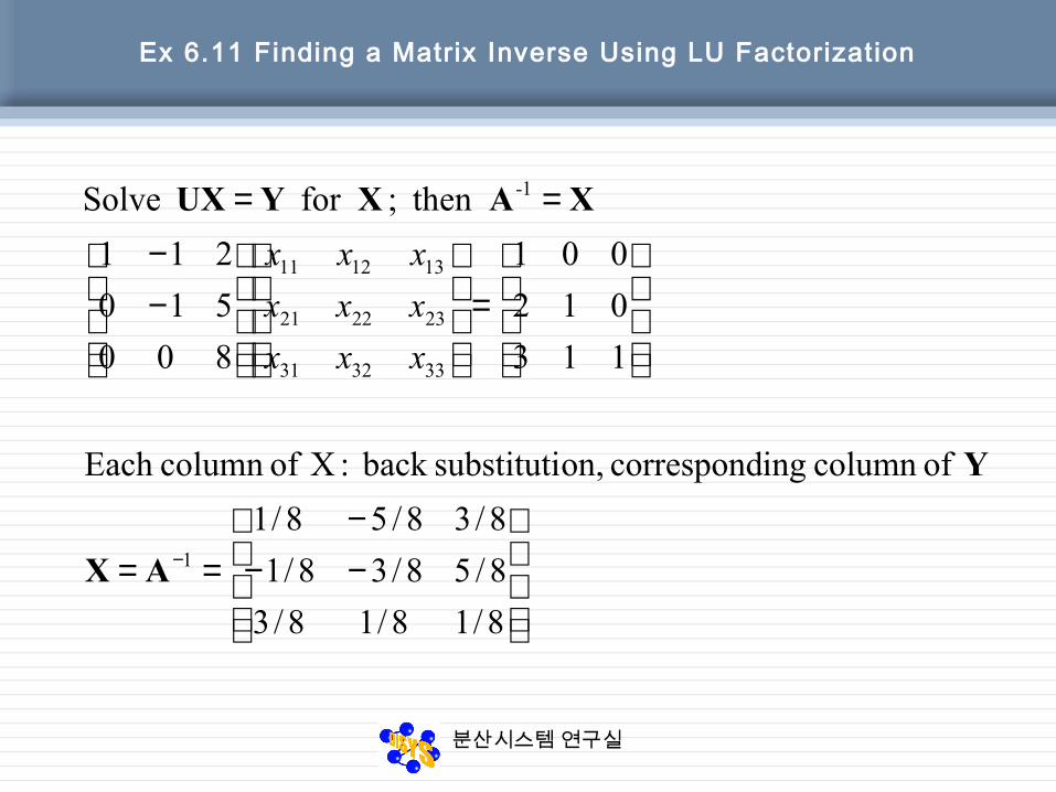
Ex 6.11 Finding a Matrix Inverse Using LU Factorization

=⇒

=

−−−

=

−−−

=

=

−−−=

=

113

012

001

0

0

1

111

012

001

ofcolumn ingcorrespond on,substituti forward : ofcolumn Each

100

010

001

111

012

001

for Solve

800

51-0

21-1

111

012

001

121-

112-

21-1

31

21

11

333231

232221

131211

Y

IY

YILY

ULA

y

y

y

yyy

yyy

yyy


Ex 6.11 Finding a Matrix Inverse Using LU Factorization

−−−

==

=

−−

==

−

8/18/18/3

8/58/38/1

8/38/58/1

ofcolumn ingcorrespond on,substitutiback : X ofcolumn Each

113

012

001

800

510

211

then ; for Solve

1

333231

232221

131211

1

AX

Y

XAXYUX

xxx

xxx

xxx

-


MATLAB Function

function x = LU_Solve_Gen(L, U, B)

% Function to solve the equation L U x = B

% L --> Lower triangular matrix (1's on diagonal)

% U --> Upper triangular matrix

% B --> Right-hand-side matrix

[n n2] = size(L); [m1 m] = size(B);

% Solve L z = B using forward substitution

for j = 1:m

z(1, j) = b(1, j);

for i = 2 : n

z(i,j) = B(i,j) - L(i, 1:i-1) * z(1:i-1, j);

end

end

% Solve U x = z using back substitution

for j = 1:m

x(n, j) = z(n, j) / U(n, n);

for i = n-1 : -1 : 1

x(i,j) = (z(i,j)-U(i,i+1:n)*x(i+1:n,j)) / U(i,i);

end

end


6.6 MATLAB’s Method


6.6 MATLAB’s Method

• 4 built- in functions– LU decomposit ion of a square matrix A

• [L, U] = lu(A), [L, U, P] = lu(A)

– Cholesky factorization• chol

– Determinant of a matrix• det

– Inverse of a matrix• inv

Education

Factorization from Gaussian Elimination