Global Positioning System in Precision Agriculture

Page 1 of 6 Global Positioning System in Precision Agriculture, A Lecture Note. Redmond Ramin Shamshiri, Ph.D. https://florida.academia.edu/RaminShamshiri

A lecture note on Global Positioning System in Precision Agriculture

Redmond Ramin Shamshiri, PhD

[email protected]

1. Introduction

There was a time when growers invested on expensive farm equipment for the sake of high technology and low energy consumption. Management assumed that sophisticated machinery were always more efficient. While this could be true to some extent, cutting-edge technologies such as precision agriculture and smart farming have opened new doors for cost-conscious farmers to apply modern management tools and to reduce the use of consumable field supplies and improve profit. Recent developments in electronic and computer has led to the invention of faster and lower-cost microprocessors that made possible manufacturing of smaller global position system (GPS) instruments and mobile based geographic information system (GIS) applications, both having great influence in precision agriculture, with significant contribution to farm management and mechanization. GPS is a satellite based navigation system that defines position, velocity and time, (PVT), under any climate condition 24 hours a day anywhere in the world, for free. Originally developed for the military, the USA owns GPS technology and the Department of Defense maintains it. GPS has made a great evolution in different aspects of our today’s modern life as well as in agriculture section. Today, a growing number of crop producers are using GPS and other modern electronic and computer equipment and practice precision agriculture. The purpose of this article is to provide a quick review of GPS concepts such as coordinate systems and NMEA standards, and to highlight some of the applications in precision agriculture. 2. Coordinate system and GPS data output

This section illustrates the basics behind GPS data collection, receivers output, data interpretation and Georeferenced data analysis. The GPS system was declared fully operational on April 27, 1995. At least 24 GPS satellites orbit the earth twice a day in a specific pattern, travelling approximately 7000 miles per hour about 12000 miles above the earth’s surface. The satellites are spaced so that they follow six orbital paths, with four satellites in each path as shown in Figure 1. This satellite arrangement guarantees that GPS receiver anywhere in the world can receive signals from at least four of them. The signals are radio waves and travel at the speed of light. It only takes between 65 and 85 milliseconds for a signal to travel from a GPS satellite to a GPS receiver. The GPS receiver collects signals from GPS satellites that are in view and uses triangulation to calculate its position, usually expressed as latitude, longitude and altitude.

Figure 1. Orbital planes and Satellite system representation

Locating a geographical point on the surface of the Earth is done

using a grid or network of latitude and longitude line, superimposed on the surface of earth. Expressing these points on a plane as a

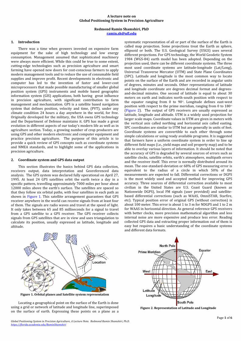
systematic representation of all or part of the surface of the Earth is called map projection. Some projections treat the Earth as sphere, ellipsoid or both. The U.S. Geological Survey (USGS) uses several different projections. For GPS technology, the World Geodetic System 1984 (WGS-84) earth model has been adopted. Depending on the projection used, there can be different coordinate systems. The three most used coordinate systems are latitude-longitude (Lat/Long), Universal Transverse Mercator (UTM) and State Plane Coordinates (SPC). Latitude and longitude is the most common way to locate points on the surface of the Earth and are recorded in angular units of degrees, minutes and seconds. Other representations of latitude and longitude coordinate are degrees decimal format and degrees-and-decimal minutes. One second of latitude is equal to about 30 meters on earth and indicates north-south position with respect to the equator ranging from 0 to 90○. Longitude defines east-west position with respect to the prime meridian, ranging from 0 to 180○ (Figure 2). The output of GPS receivers are usually expressed as latitude, longitude and altitude. UTM is a widely used projection for larger scale maps. Coordinate values in UTM are given in meters with the vertical axis called northing and horizontal axis called easting. SPC coordinates are similar to UTM but are generally in units of feet. Coordinate systems are convertible to each other through some simple calculations or using ready available programs. It is suggested that farmers have a uniform coordinate system in order to line up different field maps (i.e., yield maps and soil property map) and to be able to overlay various layers of information. It should be noted that the accuracy of GPS is degraded by several sources of errors such as satellite clocks, satellite orbits, earth’s atmosphere, multipath errors and the receiver itself. This error is normally distributed around its mean. The one-standard-deviation or 68% of GPS measuring error is equivalent to the radius of a circle in which 50% of the measurements are expected to fall. Differential corrections or DGPS is the most widely used and accepted method for improving GPS accuracy. Three sources of differential correction available to most civilian in the United States are U.S. Coast Guard (known as Nationwide DGPS), local FM signals (user provided) and satellite-based differential corrections (such as WAAS, OmniSTAR, Starfire, etc). Typical position error of original GPS (without correction) is about 100 meter. This error is about 1 to 3 m for NDGPS and 1 to 2 m for WAAS in horizontal direction. As general reference GPS receivers with better clocks, more precision mathematical algorithm and less internal noise are more expensive and produce less error. Reading collected GPS data and extracting proper information out of them is easy but requires a basic understanding of the coordinate systems and different data formats.

Figure 2. Representation of Latitude and Longitude

mailto:[email protected]


3. GPS data interpretation

GPS receiver communication is defined within an electrical data transmission standard protocol called The National Marine Electronics Association (NMEA). Most devices and programs that provide real time position information understand and expect data to be in NMEA format. A line of data called sentence or string in NMEA standard includes the entire PVT computed by GPS receiver. Different brands and categories of GPS may use different types of NMEA sentence, but all of the standard sentences always start with a ‘$’ (dollar) sign at the beginning of the line follows by GP which refers to GPS and a three letter suffix that defines the sentence contents. The data within a single line are separated by a comma and the line ends with a carriage return/line feed sequence and can be no longer than 80 characters. Common NMEA sentences used in agriculture are GPRMC, GPGGA and GPRMB.

Table 1 provides definition of each part of a data line in a GPGGA and GPRMC sentence. Once the information about different points of a field is known, parameters such as distance between points, velocity and surrounded area between three or more points can be calculated. It should be noted that for small size areas, surface of the earth can be assumed flat and distance between two points can be calculated using the normal math procedure, however spherical shape of the earth should be taken into account when two points are significantly far from each other. In this case, mathematical representation of earth model should be used.

Table 1. Interpretation of a GPRM and GPGGA sentences

$GPRMC,151739,A,2721.0310,N,08109.3878,W,001.1,343.4,101208,005.3,W*72

RMC Recommended Minimum sentence C 151739 Fix taken at 15:17:39 UTC A Status A=active or V=Void 2721.0310,N Latitude 27 deg 21.0310' N 08109.3878,W Longitude 81 deg 9.3878' W 001.1 Speed over the ground in knots 343.4 Track angle in degrees True 101208 Date – 10th of December 2008 005.3, W Magnetic Variation *7D The checksum data, always begins with * $GPGGA,152242.00,2938.4299131,N,08221.6896220,W,2,10,0.9,28.91,M,-31.11,M,5.0,0193*47 $GPGGA Global Positioning System Fix Data 152242.00 Time 15:22:42 Coordinated Universal Time (UTC) 938.4299131,N Latitude 29 deg 38.4299131' North 08221.6896220,W

Longitude 82 deg 21.6896220' West

2 Fix quality 10 Number of satellites being tracked 0.9 Horizontal dilution of position (HOD) 28.91,M Altitude, Meters, above mean sea level -31.11,M Height of Geoid (mean sea level) above WGS84 ellipsoid 5.0 time in seconds since last DGPS update 0193 DGPS station ID number *47 the checksum data, always begins with *

4. Lat/Long conversion and coordinate transformation

GPS receiver communication is defined within NMEA-0183 standard protocol. The output is an ASCII file which contains several comma delimited lines of data called sentence or string, each of which including the entire position, velocity and time (PVT) computed by the GPS receiver. Different brands use different types of NMEA sentences. As mentioned, the two most common string format used in agricultural applications are GPGGA and GPRMC. The format of latitude and longitude in both arrangements is recorded in degrees-and-decimal minutes ( ). Another way of expressing latitude and longitude is in angular units of degrees, minutes and seconds ( . It is usually necessary to convert this format to decimal degrees or radians for geometric computational purposes. This conversion is illustrated in Table 2.

Table 2. latitude and longitude conversions Decimal degrees

( ) Radian

Deg, min and decimal min

Deg, min and seconds

In order to use latitude and longitude readings of a GPS receiver

in distance calculations, they should be converted into linear units such as x and y. This conversion is complex due to the model representation of the earth (ellipsoid or sphere) and the change in point’s altitude; however when size of a farm field is small with respect to earth it can be considered as a flat surface. The purpose of transforming angular units to linear x-y coordinates is to determine the distance change corresponding to one degree of change in latitude and longitude. The following sets of calculations are based on WGS-84 spheroid earth model and can be used to calculate distance between two GPS points expressed in decimal degrees. The assumptions used in developing these equations result in errors of less than 0.1 m in 400 meter at 45 degrees latitude.

[ (

(

))]

[ (

(

))]

[ (

)

(

)

]

[ (

)

(

)

]

√

(

)

√ Eq.1

Here a=6378137 (m) is the equatorial radius, b=6356752.3142

(m) is polar radius, is elevation (m), and are true angles, and are radius of each point , , and on the X-Y coordinates, and and are the coordinates. A simple yet very accurate method to calculate distance between two points in the field is to use ellipsoidal Vincenty formula, given in Eq.2. The latitude and longitude in this method should be provided in radian format. For sufficiently close points in a field (within 1 minute change in longitude and latitude), the following equation from USGS Bulletin 1532 (1987) discussed in [3] can be used:

[ ]

Eq.2

√

[ ]

√ Eq.3


where a=6378135 (m) is the equatorial radius, b=6356752.3 (m) is the polar radius, e=0.081819803 m, Long= Longitude (rad), Lat= Latitude (rad), is the horizontal displacement, is the vertical displacement, and D is Distance (m). Another similar method is discussed in [4] and is given by the following equation:

(

[ ] )

(

[ ] )

√( ) (

) Eq.4

where Lat=Latitude (degree decimal), Long= Longitude (degree decimal), = Latitude conversion factor, = Longitude

conversion factor, and = Distance (m). To evaluate these four

methods, GPS coordinates for 11 points was collected as shown in Figure 3 and distances between each consecutive pairs were calculated and compared with tape measurement results (Table 3)

Figure 3. Experimenting with 11 sample points

Table 3. Comparison between four methods of distance calculation and validating with tape measurement

No Point (longitude, latitude) Distance (m) (Di=Pi+1-Pi) Lat Long Tape measurement Eq.1 Eq.2 Eq.3 Eq.4

1 -8108.1287 2720.2378 0.97 0.98063 0.98311 0.93232 0.95335 2 -8108.1285 2720.2373 0.98 0.98063 0.98311 0.93232 0.95335 3 -8108.1283 2720.2368 1.29 1.28970 1.29619 1.12255 1.19705 4 -8108.1279 2720.2362 1.23 1.23812 1.23919 0.94154 1.07865 5 -8108.1274 2720.2357 1.09 1.10722 1.10836 0.75813 0.92398 6 -8108.1269 2720.2353 1.37 1.37072 1.37071 0.77105 1.06992 7 -8108.1262 2720.2349 1.33 1.33239 1.33058 0.29545 0.90019 8 -8108.1254 2720.2348 1.16 1.16926 1.17175 0.27377 0.79277 9 -8108.1247 2720.2349 1.37 1.37026 1.37071 0.43727 0.95582

10 -8108.1239 2720.2351 1.16 1.16926 1.17175 0.27377 0.79277 11 -8108.1232 2720.2352 - - - - -

5. GPS application in precision agriculture

There are lots of amazing applications for GPS technology on land, at sea and in the air. GPS can be considered as the foundation of several cutting edge researches as in environmental studies, agriculture, aerospace, transportation, marine, military, surveying, recreation and so on. The GPS technology has made possible great developments in agriculture. It is used widely in precision agriculture with specific applications in crop scouting, yield mapping, field boundary mapping, soil sampling and soil property mapping, weeds and pest control and mapping, vehicle’s guidance, navigation control and so on. GPS can also help farmers to accurately identify and record their machinery locations on field and corresponding machines operational time which provides essential data in calculating field efficiency and field machine index. Data of this kind are usually huge. For example, a yield monitoring system that collects data every second generates up to tenth of thousand yield data points in a 100 acre field. This is far too much to interpret manually using paper and pencil. Computers and Geographic Information Systems (GIS) provides farmers with a powerful and exciting tool to enter, store, manipulate and display GPS collected data and associates with other data values, such as yield or soil type. This association of a data value with a geographical location or coordinate on map is called Georeferencing. These data with the same geographic coordinate displayed in different layers overlaying the same field as shown in Figure 4 afford an excellent means of farm management to reduce production cost and increase benefits. Farmers enjoying computer program can also create their own data and use GIS software to generate their own yield and soil map, however inexperienced user can easily generate misleading results. A brief illustration of how GPS is used in yield mapping and soil mapping can provide a better prospective about the application of this technology in agriculture.

Figure 4. Example of GIS layers

Traditional farmers measured crop yields for whole field or

large scales. This so called ‘collect-and-weigh’ method ignores variations that exist in soil, environmental and crop. With the GPS technology and available computers and electronic improvements, it is now possible to measure yield on much smaller scales. In determining instantaneous grain crop yield, a farmer must know three things, grain flow rate (mass/sec), combine’s travel speed and cutting width of the header or swath. Grain flow rate can be measured using grain flow sensors. Combine’s ground speed can be determined precisely from GPS receiver and can be output as a part of NMEA standard data sentence that includes latitude, longitude and vehicle heading. The yield monitoring should be programmed in a way that it properly interprets the data sentence in order to effectively use GPS as a supply of ground speed data. This instantaneous yield data can be georeferenced with coordinates of the corresponding yield data points using computer programs and create a data base to create yield map. An example of a yield map is shown in Figure 5.


Figure 5. An example of a yield map

In the absence of modern technology, soil sample was

overlooked and fertilizer was over-applied to guarantee the adequate level of nutrient for plant. There are several other factors than nutrient level that affects crop yield. Soil PH, soil organic matter, texture, topography, and compaction also have impact on crop yield. These variations in the soil should be determined through soil sampling and demonstrate as different soil property maps. As a method of soil sampling, in grid point sampling, a farmer divides a field into small size rectangular sections and gathers soil samples at the center of each grid. Along with each sample, a pair of latitude-longitude is also recorded using DGPS to georeference the properties of each soil sample. Using GIS software and interpolation, these data are then used to create soil maps as shown in Figure 6. The objective of these maps is to estimate the need for soil nutrients on a scale smaller than entire field. In large scale fields, this approach can effectively save up to several thousand dollars by adjusting fertilizer and chemicals application in different sites of the field.

Figure 6. An example of a soil map

6. GPS application in farm machinery management

Mechanical power was adopted for farm use in the late 1800’s and is a vital element in today’s modern agriculture. As the primary source of power in field, farm machinery should be used to the best possible advantage. This is an important issue as agriculture moves towards mechanization. With growth in average farm size, faster and higher capacity machines are demanded to accomplish farm tasks in a shorter time. Modern technology provides farmers with a sophisticated tool to track and monitor their equipment which in

turn increases machine productivity and labor saving. Increasing machine productivity can be achieved through optimizing effective field capacity which at the end, translates into lower unit cost of production. Two parameters play an important role in effective field machine capacity. First, machine management which refers to the mechanical condition of the machine and indicate where, when and how the machine is used on field. Second, physical condition of the field which includes field size and shape, topography, terrace layout, row length and arrangement, row-end turning space and field surface. Since a particular machine has a fixed theoretical field capacity, therefore, new technology such as GPS/GIS and wireless communication for real-time data increase machine productivity not in terms of acres per hour, but by utilizing machine and operator’s time more effectively. Track-and-record of machinery location in field using GPS is the first step in precision analysis of farm machinery operation. Processing such raw data provides useful information and document changes in machine field speed and field time that can help growers to create decision support systems for a better farm and machinery management. For example, precise determinations of time losses using GPS data along with accurate measurements and records of field speed provide an integrated tool to calculate field efficiency and machine capacity as well as visualizing driver’s performance. These results can be used to make decision on machine size and selection. In precision agriculture, GPS data are mainly used in determining some parameters of interests as in yield mapping, soil mapping, and field boundary mapping, however, this technology also provides a promising management tool in machinery management. As potential users of GPS data, farmers should know that data collection in general and data analyzing in particular provides an excellent opportunity to analyze the location and operational time of farm machinery for a better field management. Since larger machines are more expensive, their time lost such as field adjustments, loading seed and fertilizer and row ends turnings becomes more critical and more costly during annual operational hours. The increasing costs of farm operations, especially in large scale production persuade producers to invest on reliable methods of cost justification. Since mechanical power is an indispensable part of today’s agriculture, farm machinery should be used to the best possible advantage.

Operational analysis is an approach to increase machine

capacity and obtain efficient machine utilization. Driver’s performance and field condition affect total operation costs, such as fuel, lubricants and repairs, especially in larger machinery which have higher hourly costs. Another issue that is important in any farm operation and may affect farm machinery is timeliness. This parameter refers to the ability of manager to complete a farm activity at such a time that crop return (quantity and quality) is optimized. Better management strategies to improve planning and scheduling such as motion-and-time study management will reduce peak machinery demand and maintain a more stable machine force on the farm, leading to increase yield and profitability. Insufficient machine capacity may prevent completion of a field operation and create economic penalties. In some cases, the quality of field crops, including grains and hays, or horticultural crops, including vegetables and fruits are affected by the dates of planting and harvesting which represents a hidden cost associated with farm machinery. Therefore, obtaining accurate time record of all activities for a specific machine operation is always the first step in operation analysis. GPS receivers and data loggers can easily generate and store time and position information. The second step is to divide the time recorded into primary and support functions. For example, in a citrus harvesting operation, shaking tree and picking fruits from canopy is the primary function. Support functions include stops, adjustments and cleaning. Each component of operation is expresses as a percent of total field time. GPS mounted equipment and computer algorithms can provide managers with essential information for analyzing machine performance, including effective operation time. The third step is to provide details analysis of the information obtained in the steps one and two. This includes


examination of each segment of the operation to determine if the time for any appears to be excessive when compared to average values from reasonably efficient operations. Computer programs such as GIS software can be used to visualize this analysis and make decision for those segments which show the greatest possibility for improving the efficiency of the total operation.

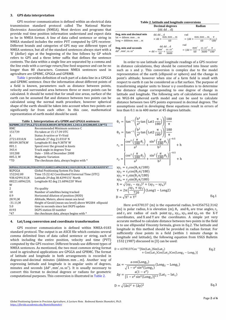
A prototype computer program (Figure 7 and Figure 8) was

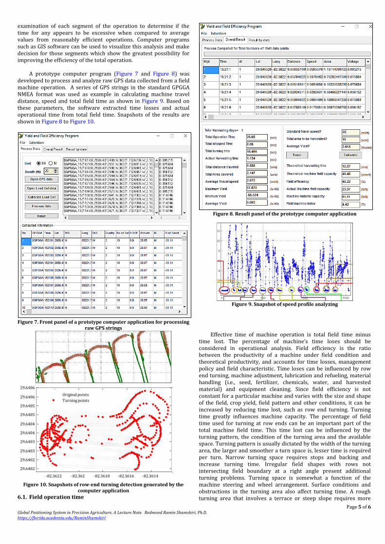
developed to process and analyze raw GPS data collected from a field machine operation. A series of GPS strings in the standard GPGGA NMEA format was used as example in calculating machine travel distance, speed and total field time as shown in Figure 9. Based on these parameters, the software extracted time losses and actual operational time from total field time. Snapshots of the results are shown in Figure 8 to Figure 10.

Figure 7. Front panel of a prototype computer application for processing

raw GPS strings

Figure 8. Result panel of the prototype computer application

Figure 9. Snapshot of speed profile analyzing

Figure 10. Snapshots of row-end turning detection generated by the

computer application

6.1. Field operation time

Effective time of machine operation is total field time minus time lost. The percentage of machine’s time loses should be considered in operational analysis. Field efficiency is the ratio between the productivity of a machine under field condition and theoretical productivity, and accounts for time losses, management policy and field characteristic. Time loses can be influenced by row end turning, machine adjustment, lubrication and refueling, material handling (i.e., seed, fertilizer, chemicals, water, and harvested material) and equipment cleaning. Since field efficiency is not constant for a particular machine and varies with the size and shape of the field, crop yield, field pattern and other conditions, it can be increased by reducing time lost, such as row end turning. Turning time greatly influences machine capacity. The percentage of field time used for turning at row ends can be an important part of the total machine field time. This time lost can be influenced by the turning pattern, the condition of the turning area and the available space. Turning pattern is usually dictated by the width of the turning area, the larger and smoother a turn space is, lesser time is required per turn. Narrow turning space requires stops and backing and increase turning time. Irregular field shapes with rows not intersecting field boundary at a right angle present additional turning problems. Turning space is somewhat a function of the machine steering and wheel arrangement. Surface conditions and obstructions in the turning area also affect turning time. A rough turning area that involves a terrace or steep slope requires more

-82.3622 -82.362 -82.3618 -82.3616 -82.3614

29.6402

29.6402

29.6403

29.6403

29.6404

29.6404

29.6405

29.6405

29.6406

29.6406

Original points

Turning points


time. Row length also has a great impact on turning time. As row length increases, turning time decreases and machine capacity increases. Field operation studies suggest that a turning of 6 to 10 percent can be obtained when fields have reasonable row length and good turn condition. A turning time of more than 10% is excessive for most operations. 6.2. Field machine index

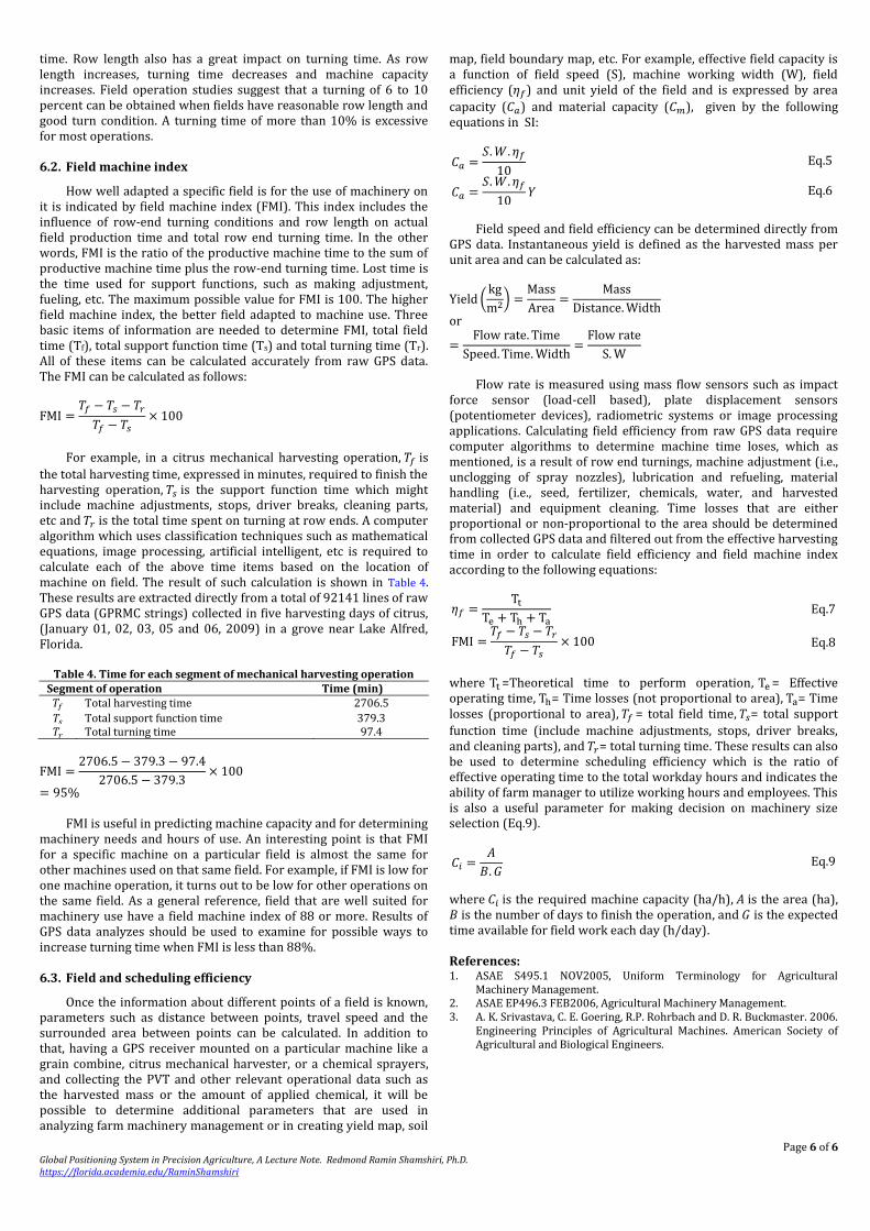
How well adapted a specific field is for the use of machinery on it is indicated by field machine index (FMI). This index includes the influence of row-end turning conditions and row length on actual field production time and total row end turning time. In the other words, FMI is the ratio of the productive machine time to the sum of productive machine time plus the row-end turning time. Lost time is the time used for support functions, such as making adjustment, fueling, etc. The maximum possible value for FMI is 100. The higher field machine index, the better field adapted to machine use. Three basic items of information are needed to determine FMI, total field time (Tf), total support function time (Ts) and total turning time (Tr). All of these items can be calculated accurately from raw GPS data. The FMI can be calculated as follows:

For example, in a citrus mechanical harvesting operation, is

the total harvesting time, expressed in minutes, required to finish the harvesting operation, is the support function time which might include machine adjustments, stops, driver breaks, cleaning parts, etc and is the total time spent on turning at row ends. A computer algorithm which uses classification techniques such as mathematical equations, image processing, artificial intelligent, etc is required to calculate each of the above time items based on the location of machine on field. The result of such calculation is shown in Table 4. These results are extracted directly from a total of 92141 lines of raw GPS data (GPRMC strings) collected in five harvesting days of citrus, (January 01, 02, 03, 05 and 06, 2009) in a grove near Lake Alfred, Florida.

Table 4. Time for each segment of mechanical harvesting operation Segment of operation Time (min) Total harvesting time 2706.5

Total support function time 379.3 Total turning time 97.4

FMI is useful in predicting machine capacity and for determining machinery needs and hours of use. An interesting point is that FMI for a specific machine on a particular field is almost the same for other machines used on that same field. For example, if FMI is low for one machine operation, it turns out to be low for other operations on the same field. As a general reference, field that are well suited for machinery use have a field machine index of 88 or more. Results of GPS data analyzes should be used to examine for possible ways to increase turning time when FMI is less than 88%. 6.3. Field and scheduling efficiency

Once the information about different points of a field is known, parameters such as distance between points, travel speed and the surrounded area between points can be calculated. In addition to that, having a GPS receiver mounted on a particular machine like a grain combine, citrus mechanical harvester, or a chemical sprayers, and collecting the PVT and other relevant operational data such as the harvested mass or the amount of applied chemical, it will be possible to determine additional parameters that are used in analyzing farm machinery management or in creating yield map, soil

map, field boundary map, etc. For example, effective field capacity is a function of field speed (S), machine working width (W), field efficiency ( ) and unit yield of the field and is expressed by area

capacity ( ) and material capacity ( ), given by the following equations in SI:

Eq.5

Eq.6

Field speed and field efficiency can be determined directly from

GPS data. Instantaneous yield is defined as the harvested mass per unit area and can be calculated as:

(

)

or

Flow rate is measured using mass flow sensors such as impact

force sensor (load-cell based), plate displacement sensors (potentiometer devices), radiometric systems or image processing applications. Calculating field efficiency from raw GPS data require computer algorithms to determine machine time loses, which as mentioned, is a result of row end turnings, machine adjustment (i.e., unclogging of spray nozzles), lubrication and refueling, material handling (i.e., seed, fertilizer, chemicals, water, and harvested material) and equipment cleaning. Time losses that are either proportional or non-proportional to the area should be determined from collected GPS data and filtered out from the effective harvesting time in order to calculate field efficiency and field machine index according to the following equations:

Eq.7

Eq.8

where =Theoretical time to perform operation, = Effective operating time, = Time losses (not proportional to area), = Time losses (proportional to area), = total field time, = total support

function time (include machine adjustments, stops, driver breaks, and cleaning parts), and = total turning time. These results can also be used to determine scheduling efficiency which is the ratio of effective operating time to the total workday hours and indicates the ability of farm manager to utilize working hours and employees. This is also a useful parameter for making decision on machinery size selection (Eq.9).

Eq.9

where is the required machine capacity (ha/h), is the area (ha), is the number of days to finish the operation, and is the expected time available for field work each day (h/day). References: 1. ASAE S495.1 NOV2005, Uniform Terminology for Agricultural

Machinery Management. 2. ASAE EP496.3 FEB2006, Agricultural Machinery Management. 3. A. K. Srivastava, C. E. Goering, R.P. Rohrbach and D. R. Buckmaster. 2006.

Engineering Principles of Agricultural Machines. American Society of Agricultural and Biological Engineers.

Education

Global Positioning System in Precision Agriculture