Embed Size (px)
Citation preview
International Journal of Advances in Engineering & Technology, Jan. 2014.
©IJAET ISSN: 22311963
2342 Vol. 6, Issue 6, pp. 2342-2353
SYSTEM IDENTIFICATION AND MODELLING OF ROTARY
INVERTED PENDULUM
T. Teng Fong, Z. Jamaludin and L. Abdullah
Faculty of Manufacturing Engineering, Universiti Teknikal Malaysia Melaka,
Durian Tunggal, 76100 Melaka, Malaysia
ABSTRACT
An inverted pendulum is a classic case of robust controller design. A successfully validated and precise system
model would greatly enhance the performance of the controller making system identification as a major
procedure in control system design. Several techniques exist in literature for system identification, and these
include time domain approach and frequency domain approach. This paper gives an in-depth analysis of system
identification and modelling of rotary inverted pendulum that describes the dynamic models in upright and
downward position. An extensive elaboration on derivation of the mathematical model describing the physical
dynamic model of the rotary inverted pendulum is described in this paper. In addition, a frequency response
function (FRF) of the physical system is measured. The parametric model estimated using non-linear least
square frequency domain identification approach based on the measured FRF is then applied as a mean to
validate the derived mathematical model. It is concluded that based on the validation, the dynamic model and
the parametric model are well fitted to the FRF measurement.
KEYWORDS: System Identification, Rotary Inverted Pendulum, Mathematical Modelling, Linear
Approximation Method, Frequency Domain Identification.
I. INTRODUCTION
Control of under-actuated systems is difficult and has attracted much attention due to their wide-
ranging applications. During the last few decades, under-actuated physical systems have drawn great
interest among researchers for developing different control strategies, such as those in robotics,
aerospace engineering, and marine engineering[1]. An inverted pendulum is a difficult system to
control being essentially unstable. Thus, control of an inverted pendulum is one of the most important
classical problems in the research interest of control engineering to improve the performance of the
control system[2]. It is a well-known fact that under-actuated systems have fewer actuators than the
degrees of freedom. The rotary inverted pendulum (RIP) system consists of an actuator and two
degrees of freedom. The pendulum is stable when hanging downwards whereas it is naturally unstable
with oscillation. Therefore, torque or force must be applied to keep it balanced to remain in inverted
position. The inverted pendulum model can be applied in control of a space booster racket and a
satellite, an automatic aircraft landing system, aircraft stabilization in the turbulent air flow,
stabilization of a cabin in a ship and others[3].
Mathematical modelling, simulation, non-linear analysis, decision making, identification, estimation,
diagnostics, and optimization have become major mainstreams in control system engineering. System
identification is a general term used to describe mathematical tools and algorithms that build
dynamical models from measured data[4]. Mathematical modelling is the basis of the control
strategies when approaching the solution of a control problem. The physical system dynamic
equations were performed analytically or numerically in solving these equations. It can be derived by
the Newtonian mechanics and the Lagrange’s equations of motion, the Kirchhoff’s laws, and the
International Journal of Advances in Engineering & Technology, Jan. 2014.
©IJAET ISSN: 22311963
2343 Vol. 6, Issue 6, pp. 2342-2353
energy conservation principles[5]. There are many approaches when deriving the mathematical
model, but Lagrange equations offer the systematic and error free way to do it[6]. The equations of
motion normally were obtained by using the free body diagram referencing to Newtonian method.
Linearization the non-linear model with single support point was possible performed about
equilibrium point[7]. Then, the linear control theories can be applied in design and control the system.
Besides that, the MATLAB GUI can be used to estimate automatically the mathematical model of the
system[8]. Furthermore, parametric model, non-parametric model, black box model, white box model
and linear model can be applied in system identification. The system identification was estimated
using non-linear least square frequency domain identification method and H1 estimator in frequency
response function (FRF)[9]. The frequency domain identification method offers several advantages
compared to the time domain approach, such as data and noise reduction[10].
The aim of this paper is to extensively elaborate the identification and modelling of a rotary inverted
pendulum using mathematical model validated with parametric model generated using frequency
response function. The paper is organized as follows; the next section provides the system setup.
Section III shows the methodology of mathematical modelling and frequency response method
together with the validation result and discussion. Finally, a conclusion and future work are given in
Section IV of the paper.
II. SYSTEM SETUP
TeraSoft Electro-Mechanical Engineering Control System (EMECS) is a set of electro-mechanical
devices for controlling engineering research and education. The EMECS consists of three main
components such as Micro-box 2000/2000C, servo-motor module, and driver circuit. The Micro-box
2000/2000C is a xPC Target machine that operates on wide variety of x86-based PC system where the
system has analogue-to-digital converter (ADC), digital-to-analogue converter (DAC), general-
purpose input/output (GPIO) and encoder input/output boards installed. It works as data acquisition
unit with operating voltage between 9 and 36 volts. Then, the servo-motor module consists of a
permanent-magnet, brushed DC motor that runs on a terminal voltage of 24 volts. Besides that,
angular position of shaft of the DC motor is measured by a rotary incremental optical encoder. The
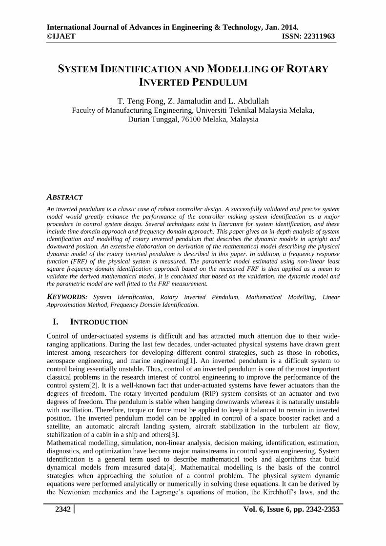
encoder has a resolution of 500 counts per resolution. Figure 1 shows a schematic diagram of EMECS
that includes the servo-motor module, driver circuit, Micro-box 2000/2000C and host computer. The
driver circuit and the servo-motor module are connected to the Micro-Box 2000/2000C. The
switching power supply is connected to the driver circuit board and AC/DC adapter is connected to
the data acquisition unit. Besides, Ethernet cable is connected between host computer and the data
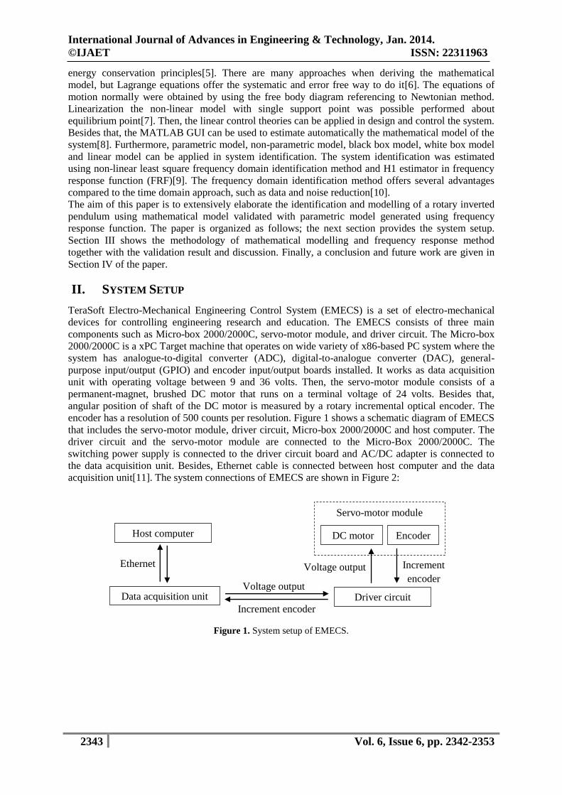
acquisition unit[11]. The system connections of EMECS are shown in Figure 2:
Figure 1. System setup of EMECS.
Increment encoder
Increment
encoder Voltage output
Voltage output
Ethernet
Host computer
Data acquisition unit
Servo-motor module
Driver circuit
Encoder DC motor
International Journal of Advances in Engineering & Technology, Jan. 2014.
©IJAET ISSN: 22311963
2344 Vol. 6, Issue 6, pp. 2342-2353
Figure 2. System connections of EMECS.
III. RESEARCH METHODOLOGY
The methodology of identification of system is described using two different methods which are
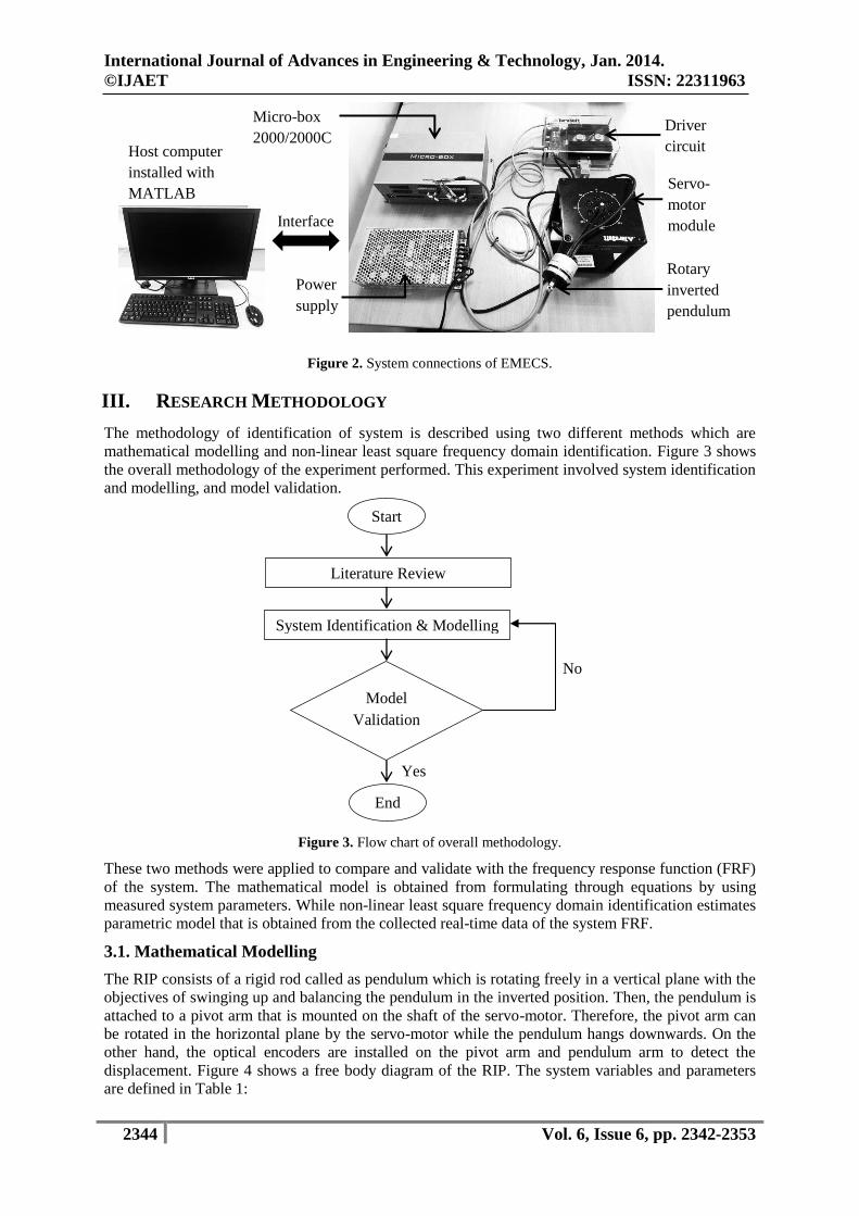
mathematical modelling and non-linear least square frequency domain identification. Figure 3 shows
the overall methodology of the experiment performed. This experiment involved system identification
and modelling, and model validation.
Figure 3. Flow chart of overall methodology.
These two methods were applied to compare and validate with the frequency response function (FRF)
of the system. The mathematical model is obtained from formulating through equations by using
measured system parameters. While non-linear least square frequency domain identification estimates
parametric model that is obtained from the collected real-time data of the system FRF.
3.1. Mathematical Modelling
The RIP consists of a rigid rod called as pendulum which is rotating freely in a vertical plane with the
objectives of swinging up and balancing the pendulum in the inverted position. Then, the pendulum is
attached to a pivot arm that is mounted on the shaft of the servo-motor. Therefore, the pivot arm can
be rotated in the horizontal plane by the servo-motor while the pendulum hangs downwards. On the
other hand, the optical encoders are installed on the pivot arm and pendulum arm to detect the
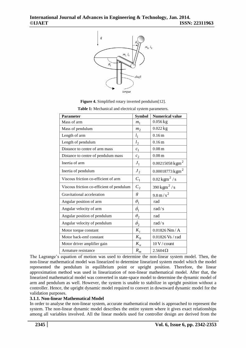
displacement. Figure 4 shows a free body diagram of the RIP. The system variables and parameters
are defined in Table 1:
Yes
No
Start
Literature Review
System Identification & Modelling
Model
Validation
End
Interface
Host computer
installed with
MATLAB
Simulink software
Power
supply
Driver
circuit
Micro-box
2000/2000C
Servo-
motor
module
Rotary
inverted
pendulum
International Journal of Advances in Engineering & Technology, Jan. 2014.
©IJAET ISSN: 22311963
2345 Vol. 6, Issue 6, pp. 2342-2353
Figure 4. Simplified rotary inverted pendulum[12].
Table 1: Mechanical and electrical system parameters.
Parameter Symbol Numerical value
Mass of arm 1m 0.056 kg
Mass of pendulum 2m 0.022 kg
Length of arm 1l 0.16 m
Length of pendulum 2l 0.16 m
Distance to centre of arm mass 1c 0.08 m
Distance to centre of pendulum mass 2c
0.08 m
Inertia of arm 1J 0.00215058
2kgm
Inertia of pendulum 2J 0.00018773
2kgm
Viscous friction co-efficient of arm 1C 0.02 s/kgm2
Viscous friction co-efficient of pendulum 2C 390 s/kgm2
Gravitational acceleration g 9.8
2s/m
Angular position of arm 1 rad
Angular velocity of arm 1
s/rad
Angular position of pendulum 2 rad
Angular velocity of pendulum 2
s/rad
Motor torque constant tK 0.01826 A/Nm
Motor back-emf constant bK 0.01826 rad/Vs
Motor driver amplifier gain uK
10 count/V
Armature resistance mR 2.5604
The Lagrange’s equation of motion was used to determine the non-linear system model. Then, the
non-linear mathematical model was linearized to determine linearized system model which the model
represented the pendulum in equilibrium point or upright position. Therefore, the linear
approximation method was used in linearization of non-linear mathematical model. After that, the
linearized mathematical model was converted in state-space model to determine the dynamic model of
arm and pendulum as well. However, the system is unable to stabilize in upright position without a
controller. Hence, the upright dynamic model required to convert in downward dynamic model for the
validation purposes.
3.1.1. Non-linear Mathematical Model
In order to analyse the non-linear system, accurate mathematical model is approached to represent the
system. The non-linear dynamic model describes the entire system where it gives exact relationships
among all variables involved. All the linear models used for controller design are derived from the
International Journal of Advances in Engineering & Technology, Jan. 2014.
©IJAET ISSN: 22311963
2346 Vol. 6, Issue 6, pp. 2342-2353
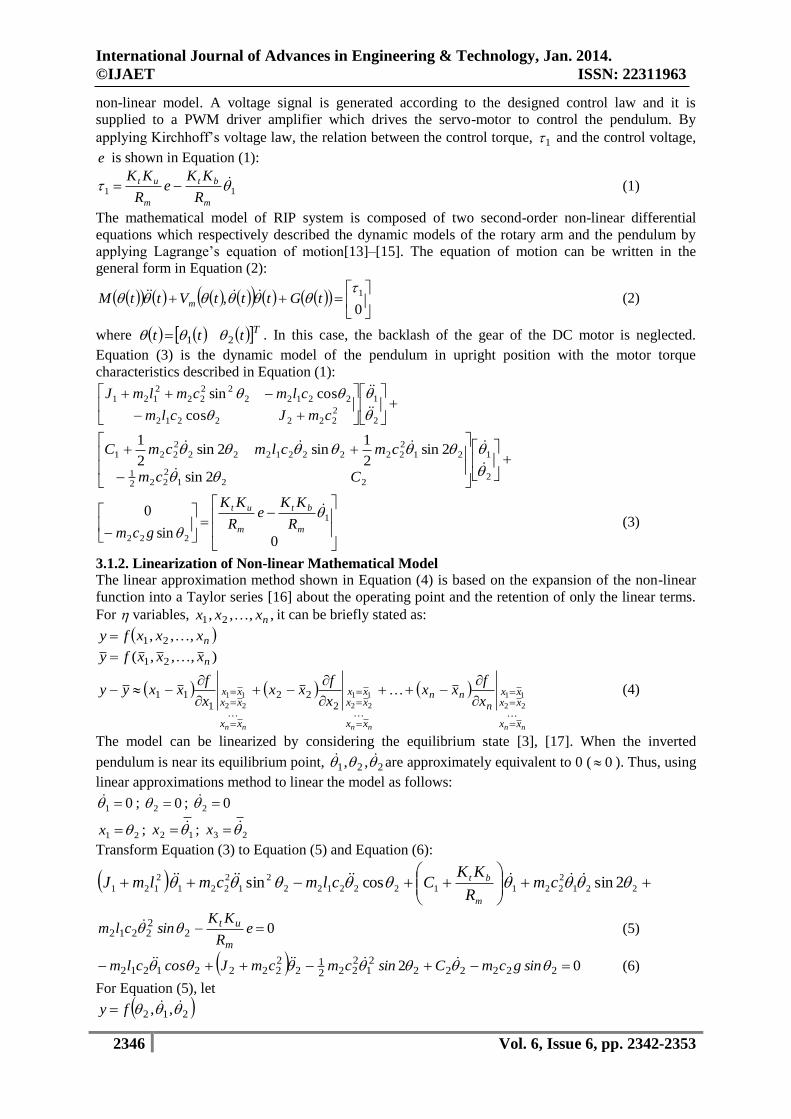
non-linear model. A voltage signal is generated according to the designed control law and it is
supplied to a PWM driver amplifier which drives the servo-motor to control the pendulum. By
applying Kirchhoff’s voltage law, the relation between the control torque, 1 and the control voltage,
e is shown in Equation (1):
11
m
bt
m
ut
R
KKe
R
KK (1)
The mathematical model of RIP system is composed of two second-order non-linear differential
equations which respectively described the dynamic models of the rotary arm and the pendulum by
applying Lagrange’s equation of motion[13]–[15]. The equation of motion can be written in the
general form in Equation (2):
0,
1 tGtttVttM m
(2)
where Tttt 21 . In this case, the backlash of the gear of the DC motor is neglected.
Equation (3) is the dynamic model of the pendulum in upright position with the motor torque
characteristics described in Equation (1):
2
1
22222212
2212222
222121
cos
cossin
cmJclm
clmcmlmJ
2
1
2212222
1
212222221222
2221
2sin
2sin2
1sin2sin
2
1
Ccm
cmclmcmC
0
sin
01
222
m
bt
m
ut
R
KKe
R
KK
gcm (3)
3.1.2. Linearization of Non-linear Mathematical Model
The linear approximation method shown in Equation (4) is based on the expansion of the non-linear
function into a Taylor series [16] about the operating point and the retention of only the linear terms.
For variables, ,,,, 21 nxxx it can be briefly stated as:
nxxxfy ,,, 21 ),,,( 21 nxxxfy
nnnnnn xx
xxxx
nnn
xx
xxxx
xx
xxxx
x
fxx
x
fxx
x
fxxyy
22
11
22
11
22
11
222
111 (4)
The model can be linearized by considering the equilibrium state [3], [17]. When the inverted
pendulum is near its equilibrium point, 221 ,, are approximately equivalent to 0 ( 0 ). Thus, using
linear approximations method to linear the model as follows:
01 ; 02 ; 02
21 x ; 12 x ; 23 x
Transform Equation (3) to Equation (5) and Equation (6):
221
2
2211222122
2
1
2
221
2
121 2sin cossin cmR
KKCclmcmlmJ
m
bt
0222212 e
R
KKsinclm
m
ut (5)
02 2222222
12222
12
222221212 singcmCsincmcmJcosclm (6)
For Equation (5), let
212 ,, fy
International Journal of Advances in Engineering & Technology, Jan. 2014.
©IJAET ISSN: 22311963
2347 Vol. 6, Issue 6, pp. 2342-2353
221
22211222122
21
2221
2121 2 sincm
R
KKCcosclmsincmlmJy
m
bt
eR
KKsinclm
m
ut222212 (7)
0,0,0,, 212 ffy
eR
KKclmlmJy
m
ut 221212121
(8)
222212221
22222212221
222
2
cos2cos2sincossin2
clmcmclmcmy
0
0
0
02
2
1
2
y (9)
222221
1
2
sincmR
KKC
y
m
bt
m
bt
R
KKC
y
1
0
0
01
2
1
2
(10)
2221221222
2
sin22sin
clmcmy
0
0
0
02
2
1
2
y
(11)
0
0
02
2
0
0
01
1
0
0
02
2
2
1
2
2
1
2
2
1
2000
yyy
yy
1122121
2
121
m
bt
m
ut
R
KKCe
R
KKclmlmJy (12)
Therefore, Equation (13) is linearized Equation (5) yields:
0 1122121
2
121
e
R
KK
R
KKCclmlmJ
m
ut
m
bt (13)
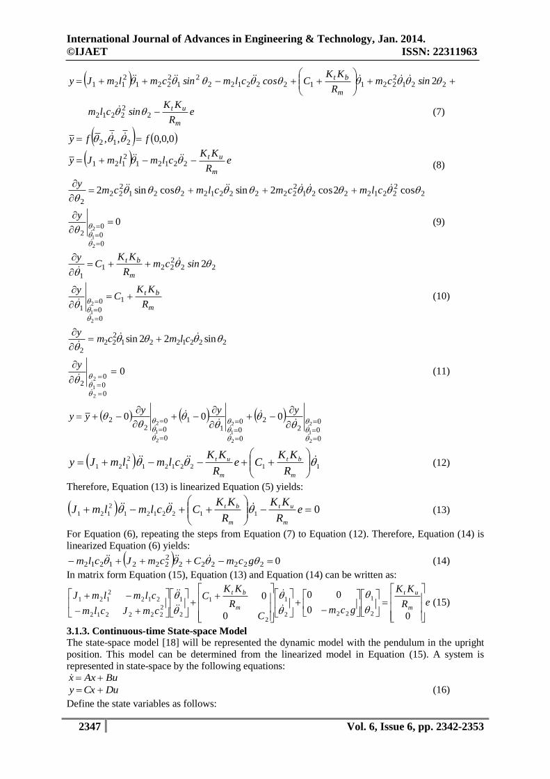
For Equation (6), repeating the steps from Equation (7) to Equation (12). Therefore, Equation (14) is
linearized Equation (6) yields:
022222222221212 gcmCcmJclm (14)
In matrix form Equation (15), Equation (13) and Equation (14) can be written as:
eR
KK
gcmC
R
KKC
cmJclm
clmlmJm
ut
m
bt
00
00
0
0
2
1
222
1
2
1
2
1
2222212
2122121
(15)
3.1.3. Continuous-time State-space Model
The state-space model [18] will be represented the dynamic model with the pendulum in the upright
position. This model can be determined from the linearized model in Equation (15). A system is
represented in state-space by the following equations: BuAxx
DuCxy (16)
Define the state variables as follows:

International Journal of Advances in Engineering & Technology, Jan. 2014.
©IJAET ISSN: 22311963
2348 Vol. 6, Issue 6, pp. 2342-2353
TTxxxx 21214321
uR
KKx
R
KKCxclmxlmJ
m
ut
m
bt
3142123
2
121 (17)
022242422223212 gxcmxCxcmJxclm (18)
Solve the two variables equations using substitution method to eliminate one of the variables by
replacement when solving a system of equations. For Equation (18), let
2222
2224232124
cmJ
gxcmxCxclmx
(19)
Substitute Equation (19) in Equation (17), 3x yields Equation (20):
22
21
22
2222
2121
22222
221
2231
222242212
3clmcmJlmJ
uR
KKcmJgxclmx
R
KKCcmJxCclm
xm
ut
m
bt
(20)
For Equation (18), let
212
2224242222
3clm
gxcmxCxcmJx
(21)
Substitute Equation (21) in Equation (17), 4x yields Equation (22):
22
21
22
2222
2121
21222221213121242
2121
4clmcmJlmJ
uR
KKclmxgcmlmJx
R
KKCclmxClmJ
xm
ut
m
bt
(22)
With the physical parameters of the system mentioned above, the state-space model is represented the
linearized system in upright position as stated in equation (24):
31 xx
42 xx
22
21
22
2222
2121
22222
221
2231
222242212
3clmcmJlmJ
uR
KKcmJgxclmx
R
KKCcmJxCclm
xm
ut
m
bt
22
21
22
2222
2121
21222221213121242
2121
4clmcmJlmJ
uR
KKclmxgcmlmJx
R
KKCclmxClmJ
xm
ut
m
bt
(23)
u
x
x
x
x
x
x
x
x
7236.24
8442.28
0
0
0584.19788.66254.570
1098.01419.89796.50
1000
0100
4
3
2
1
4
3
2
1
4
3
2
1
0010
x
x
x
x
y (24)
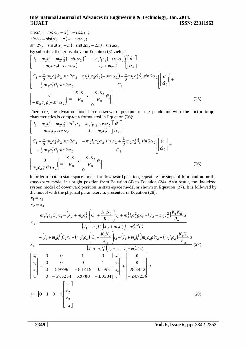
In addition, the dynamic model for downward position of pendulum is formulated in the following
formulas. Defined 2 to be the angular position of the pendulum that taken from the downward
vertical. Thus, the relationship between terms involving 2 and 2 can be well defined as follows:
22 ; 22 ; 22 ;
International Journal of Advances in Engineering & Technology, Jan. 2014.
©IJAET ISSN: 22311963
2349 Vol. 6, Issue 6, pp. 2342-2353
222 coscoscos ;
222 sinsinsin ;
2222 2sin22sin2sin2sin
By substitute the terms above in Equation (3) yields:
2
1
22222212
22122
2222
2121
cmJcosclm
cosclmsincmlmJ
2
1
2212222
1
212222221222
2221
2
22
12
2
1
Csincm
sincmsinclmsincmC
0
01
222
m
bt
m
ut
R
KKe
R
KK
singcm (25)
Therefore, the dynamic model for downward position of the pendulum with the motor torque
characteristics is compactly formulated in Equation (26):
2
1
22222212
2212222
222121
cmJcosclm
cosclmsincmlmJ
2
1
2212222
1
212222221222
2221
2
22
12
2
1
Csincm
sincmsinclmsincmC
0
01
222
m
bt
m
ut
R
KKe
R
KK
singcm (26)
In order to obtain state-space model for downward position, repeating the steps of formulation for the
state-space model in upright position from Equation (4) to Equation (24). As a result, the linearized
system model of downward position in state-space model as shown in Equation (27). It is followed by
the model with the physical parameters as presented in Equation (28):
31 xx
42 xx
22
21
22
2222
2121
22222
221
2231
222242212
3clmcmJlmJ
uR
KKcmJgxclmx
R
KKCcmJxCclm
xm
ut
m
bt
22
21
22
2222
2121
21222221213121242
2121
4clmcmJlmJ
uR
KKclmxgcmlmJx
R
KKCclmxClmJ
xm
ut
m
bt
(27)
u
.
.
x
x
x
x
...
...
x
x
x
x
723624
844228
0
0
05841978866254570
1098014198979650
1000
0100
4
3
2
1
4
3
2
1
4
3
2
1
0010
x
x
x
x
y (28)
International Journal of Advances in Engineering & Technology, Jan. 2014.
©IJAET ISSN: 22311963
2350 Vol. 6, Issue 6, pp. 2342-2353
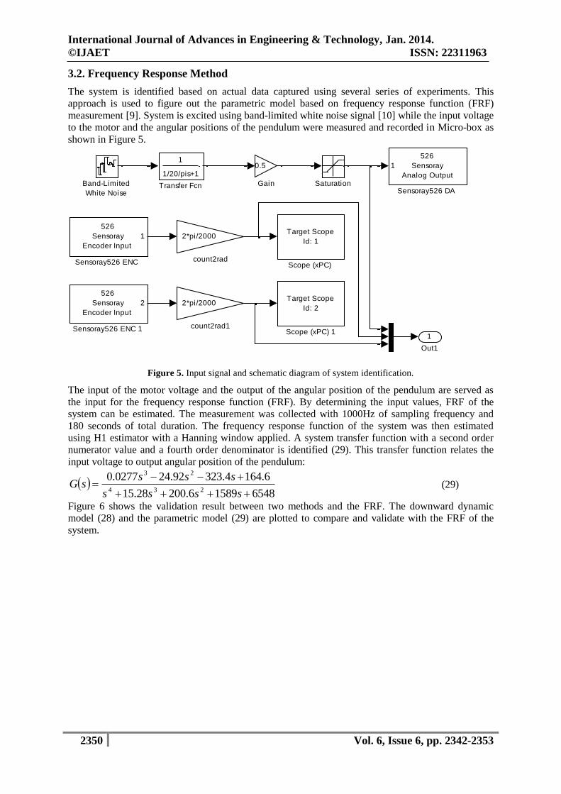
3.2. Frequency Response Method
The system is identified based on actual data captured using several series of experiments. This
approach is used to figure out the parametric model based on frequency response function (FRF)
measurement [9]. System is excited using band-limited white noise signal [10] while the input voltage
to the motor and the angular positions of the pendulum were measured and recorded in Micro-box as
shown in Figure 5.
1
Out1
2*pi/2000
count2rad1
2*pi/2000
count2rad
1
1/20/pis+1
Transfer Fcn
526
Sensoray
Encoder Input
2
Sensoray526 ENC 1
526
Sensoray
Encoder Input
1
Sensoray526 ENC
526
Sensoray
Analog Output
1
Sensoray526 DA
Target Scope
Id: 2
Scope (xPC) 1
Target Scope
Id: 1
Scope (xPC)
Saturation
0.5
GainBand-Limited
White Noise
Figure 5. Input signal and schematic diagram of system identification.
The input of the motor voltage and the output of the angular position of the pendulum are served as
the input for the frequency response function (FRF). By determining the input values, FRF of the
system can be estimated. The measurement was collected with 1000Hz of sampling frequency and
180 seconds of total duration. The frequency response function of the system was then estimated
using H1 estimator with a Hanning window applied. A system transfer function with a second order
numerator value and a fourth order denominator is identified (29). This transfer function relates the
input voltage to output angular position of the pendulum:
654815896.20028.15
6.1644.32392.240277.0234
23
ssss
ssssG (29)
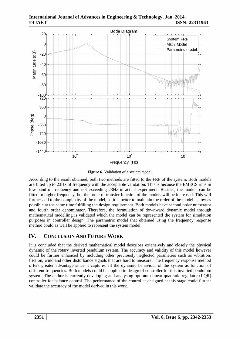
Figure 6 shows the validation result between two methods and the FRF. The downward dynamic
model (28) and the parametric model (29) are plotted to compare and validate with the FRF of the
system.
International Journal of Advances in Engineering & Technology, Jan. 2014.
©IJAET ISSN: 22311963
2351 Vol. 6, Issue 6, pp. 2342-2353
-100
-80
-60
-40
-20
0
20M
ag
nitu
de
(d
B)
100
101
102
-1440
-1080
-720
-360
0
360
720
Ph
ase
(d
eg
)Bode Diagram
Frequency (Hz)
System FRF
Math. Model
Parametric model
Figure 6. Validation of a system model.
According to the result obtained, both two methods are fitted to the FRF of the system. Both models
are fitted up to 23Hz of frequency with the acceptable validation. This is because the EMECS runs in
low band of frequency and not exceeding 23Hz in actual experiment. Besides, the models can be
fitted to higher frequency, but the order of transfer function of the models will be increased. This will
further add to the complexity of the model, so it is better to maintain the order of the model as low as
possible at the same time fulfilling the design requirement. Both models have second order numerator
and fourth order denominator. Therefore, the formulation of downward dynamic model through
mathematical modelling is validated which the model can be represented the system for simulation
purposes in controller design. The parametric model that obtained using the frequency response
method could as well be applied to represent the system model.
IV. CONCLUSION AND FUTURE WORK
It is concluded that the derived mathematical model describes extensively and closely the physical
dynamic of the rotary inverted pendulum system. The accuracy and validity of this model however
could be further enhanced by including other previously neglected parameters such as vibration,
friction, wind and other disturbance signals that are hard to measure. The frequency response method
offers greater advantage since it captures all the dynamic behaviour of the system as function of
different frequencies. Both models could be applied in design of controller for this inverted pendulum
system. The author is currently developing and analysing optimum linear quadratic regulator (LQR)
controller for balance control. The performance of the controller designed at this stage could further
validate the accuracy of the model derived in this work.
International Journal of Advances in Engineering & Technology, Jan. 2014.
©IJAET ISSN: 22311963
2352 Vol. 6, Issue 6, pp. 2342-2353
V. ACKNOWLEDGEMENTS
The authors would like to thank the Faculty of Manufacturing Engineering, Universiti Teknikal
Malaysia Melaka (UTeM) that provided the laboratory facilities and equipment supports. Also, this
research is supported by the scholarship from the Centre for Graduate Studies of the Universiti
Teknikal Malaysia Melaka (UTeM).
REFERENCES
[1] N. S. Ozbek & M. O. Efe, (2010) “Swing up and stabilization control experiments for a rotary inverted
pendulum— An educational comparison”, in 2010 IEEE International Conference on Systems, Man
and Cybernetics, pp. 2226–2231.
[2] L. B. Prasad, B. Tyagi & H. O. Gupta, (2011) “Optimal control of nonlinear inverted pendulum
dynamical system with disturbance input using PID controller & LQR”, in 2011 IEEE International
Conference on Control System, Computing and Engineering, pp. 540–545.
[3] K. Barya & S. Tiwari, (2010) “Comparison of LQR and Robust Controllers for stabilizing Inverted
Pendulum System”, in 2010 IEEE International Conference on Communication Control and
Computing Technologies (ICCCCT), pp. 300–304.
[4] J. Pintelon, R. & Schoukens (2012) System identification: A frequency domain approach – 2nd edition.
John Wiley & Sons, Inc.
[5] M. Akhtaruzzaman & A. A. Shafie, (2010) “Modeling and control of a rotary inverted pendulum using
various methods, comparative assessment and result analysis”, in 2010 IEEE International Conference
on Mechatronics and Automation, pp. 1342–1347.
[6] P. Ernest & P. Horacek, (2011) “Algorithms for control of a rotating pendulum,” in Proc. of the 19th
IEEE Mediterranean Conf. on Control and Aut (MED’11), Corfu, Greece. 2011, no. 102.
[7] P. Xue & W. Wei, (2010) “An Analysis on the Kinetic Model of a Rotary Inverted Pendulum, and Its
Intelligent Control”, in 2010 International Conference on Computational and Information Sciences, pp.
978–981.
[8] S. Jadlovska & J. Sarnovsky, (2012) “A complex overview of the rotary single inverted pendulum
system,” in 2012 ELEKTRO, pp. 305–310.
[9] T. H. Chiew, Z. Jamaludin, A. Y. B. Hashim, N. A. Rafan & L. Abdullah, (2013) “Identification of
Friction Models for Precise Positioning System in Machine Tools”, in Procedia Engineering, vol. 53,
pp. 569–578.
[10] L. Abdullah, Z. Jamaludin, T. H. Chiew, N. A. Rafan & M. S. S. Mohamed, (2012) “System
Identification of XY Table Ballscrew Drive Using Parametric and Non Parametric Frequency Domain
Estimation Via Deterministic Approach”, in Procedia Engineering, vol. 41, no. Iris, pp. 567–574.
[11] Solution4U (2009) Electro-Mechanical Engineering Control System user’s manual, TeraSoft, Inc.
[12] A. A. Shojaei, M. F. Othman, R. Rahmani & M. R. Rani, (2011) “A Hybrid Control Scheme for a
Rotational Inverted Pendulum”, in 2011 UKSim 5th European Symposium on Computer Modeling and
Simulation, pp. 83–87.
[13] S. Anvar, (2010) “Design and implementation of sliding mode-state feedback control for stabilization
of Rotary Inverted Pendulum”, in 2010 International Conference on Control Automation and Systems
(ICCAS), pp. 1952–1957.
[14] J. A. Acosta, (2010) “Furuta’s Pendulum: A Conservative Nonlinear Model for Theory and Practise”,
Math. Probl. Eng., vol. 2010, pp. 1–29.
[15] J.-H. Li, (2013) “Composite fuzzy control of a rotary inverted pendulum”, in 2013 IEEE International
Symposium on Industrial Electronics, pp. 1–5.
[16] S. Jadlovska & J. Sarnovsky, (2013) “Application of the state-dependent Riccati equation method in
nonlinear control design for inverted pendulum systems”, in 2013 IEEE 11th International Symposium
on Intelligent Systems and Informatics (SISY), vol. 0, no. 1, pp. 209–214.
[17] P. Kumar, O. N. Mehrotra & J. Mahto, (2013) “Classical , Smart And Modern Controller Design Of
Inverted Pendulum”, Int. J. Eng. Res. Appl., vol. 3, no. 2, pp. 1663–1672.
[18] A. Rybovic, M. Priecinsky, M. Paskala & A. Mechanical, (2012) “Control of the Inverted Pendulum
Using State Feedback Control,” in 2012 ELEKTRO, pp. 145–148.

International Journal of Advances in Engineering & Technology, Jan. 2014.
©IJAET ISSN: 22311963
2353 Vol. 6, Issue 6, pp. 2342-2353
AUTHORS
Tang Teng Fong received the B.Eng. degree in manufacturing engineering from Universiti
Teknikal Malaysia Melaka, Durian Tunggal, Malaysia, in 2012. He is currently pursuing
M.Sc. degree in manufacturing engineering from Universiti Teknikal Malaysia Melaka,
Durian Tunggal, Malaysia. His field of study is in control systems.
Zamberi Jamaludin, received the B.Eng. degree in chemical engineering from Lakehead
University, Thunder Bay, Ontario, Canada, in 1997, the M.Eng. degree in manufacturing
systems from National University of Malaysia, Bangi, Malaysia, in 2001, and the Ph.D.
degree in engineering from Katholieke Universiteit Leuven, Leuven, Belgium, in 2008. He
is currently a Senior Lecturer with the Department of Robotic and Automation, Faculty of
Manufacturing Engineering, Universiti Teknikal Malaysia Melaka, Durian Tunggal,
Malaysia. His fields of interest are in control systems, motion control, mechatronics, and
robotics.
Lokman Abdullah received the B.Eng. degree in manufacturing engineering from
International Islamic University Malaysia, Selayang, Malaysia, in 2005, the M.Sc. degree in
manufacturing system engineering from Coventry University, Coventry, United Kingdom,
in 2008. He is currently a Lecturer with the Department of Robotic and Automation,
Faculty of Manufacturing Engineering, Universiti Teknikal Malaysia Melaka, Durian
Tunggal, Malaysia. His fields of interest are in control systems and RFID.


![Inverted Pendulum [Final]](https://img.pdfslide.net/doc/110x75/58904db31a28abcb668bcda8/inverted-pendulum-final.jpg)