08 Machine Learning Maximum Aposteriori

Machine Learning for Data MiningMaximum A Posteriori (MAP)

Andres Mendez-Vazquez

July 22, 2015

1 / 66

Outline

1 IntroductionA first solutionExampleProperties of the MAP

2 Example of Application of MAP and EMExampleLinear RegressionThe Gaussian NoiseA Hierarchical-Bayes View of the Laplacian PriorSparse Regression via EMJeffrey’s Prior

2 / 66

Introduction

We go back to the Bayesian Rule

p (Θ|X ) = p (X|Θ) p (Θ)p (X ) (1)

We now seek that value for Θ, called Θ̂MAP

It allows to maximize the posterior p (Θ|X )

3 / 66

Introduction

We go back to the Bayesian Rule

p (Θ|X ) = p (X|Θ) p (Θ)p (X ) (1)

We now seek that value for Θ, called Θ̂MAP

It allows to maximize the posterior p (Θ|X )

3 / 66

Outline



4 / 66

Development of the solution

We look to maximize Θ̂MAP

Θ̂MAP = argmaxΘ

p (Θ)

= argmaxΘ

p (X|Θ) p (Θ)P (X )

≈ argmaxΘ

p (X|Θ) p (Θ)

= argmaxΘ

∏xi∈X

p (xi |Θ) p (Θ)

P (X ) can be removed because it has no functional relation with Θ.

5 / 66



Θ̂MAP = argmaxΘ

p (Θ)

= argmaxΘ

p (X|Θ) p (Θ)P (X )

≈ argmaxΘ

p (X|Θ) p (Θ)

= argmaxΘ

∏xi∈X

p (xi |Θ) p (Θ)


5 / 66



Θ̂MAP = argmaxΘ

p (Θ)

= argmaxΘ

p (X|Θ) p (Θ)P (X )

≈ argmaxΘ

p (X|Θ) p (Θ)

= argmaxΘ

∏xi∈X

p (xi |Θ) p (Θ)


5 / 66



Θ̂MAP = argmaxΘ

p (Θ)

= argmaxΘ

p (X|Θ) p (Θ)P (X )

≈ argmaxΘ

p (X|Θ) p (Θ)

= argmaxΘ

∏xi∈X

p (xi |Θ) p (Θ)


5 / 66



Θ̂MAP = argmaxΘ

p (Θ)

= argmaxΘ

p (X|Θ) p (Θ)P (X )

≈ argmaxΘ

p (X|Θ) p (Θ)

= argmaxΘ

∏xi∈X

p (xi |Θ) p (Θ)


5 / 66

We can make this easier

Use logarithms

Θ̂MAP = argmaxΘ

∑xi∈X

log p (xi |Θ) + log p (Θ)

(2)

6 / 66

Outline



7 / 66

What Does the MAP Estimate Get

Something NotableThe MAP estimate allows us to inject into the estimation calculation ourprior beliefs regarding the parameters values in Θ.

For exampleLet’s conduct N independent trials of the following Bernoulli experimentwith q parameter:

We will ask each individual we run into in the hallway whether theywill vote PRI or PAN in the next presidential election.

With probability p to vote PRIWhere the values of xi is either PRI or PAN.

8 / 66






8 / 66






8 / 66






8 / 66

First the ML estimateSamples

X ={

xi ={

PANPRI

i = 1, ...,N}

(3)

The log likelihood function

log P (X|p) =N∑

i=1log p (xi |q)

=∑

ilog p (xi = PRI |q) + ...∑

ilog p (xi = PAN |1− q)

=nPRI log q + (N − nPRI ) log (1− q)

Where nPRI are the numbers of individuals who are planning to vote PRIthis fall 9 / 66


X ={

xi ={

PANPRI

i = 1, ...,N}

(3)


log P (X|p) =N∑

i=1log p (xi |q)

=∑






X ={

xi ={

PANPRI

i = 1, ...,N}

(3)


log P (X|p) =N∑

i=1log p (xi |q)

=∑






X ={

xi ={

PANPRI

i = 1, ...,N}

(3)


log P (X|p) =N∑

i=1log p (xi |q)

=∑






X ={

xi ={

PANPRI

i = 1, ...,N}

(3)


log P (X|p) =N∑

i=1log p (xi |q)

=∑





We use our classic tricks

By setting

L = log P (X|q) (4)

We have that∂L∂q = 0 (5)

ThusnPRI

q − (N − nPRI )(1− q) = 0 (6)

10 / 66


By setting

L = log P (X|q) (4)


ThusnPRI

q − (N − nPRI )(1− q) = 0 (6)

10 / 66


By setting

L = log P (X|q) (4)


ThusnPRI

q − (N − nPRI )(1− q) = 0 (6)

10 / 66

Final Solution of ML

We get

q̂PRI = nPRIN (7)

ThusIf we say that N = 20 and if 12 are going to vote PRI, we get q̂PRI = 0.6.

11 / 66

Final Solution of ML

We get

q̂PRI = nPRIN (7)

ThusIf we say that N = 20 and if 12 are going to vote PRI, we get q̂PRI = 0.6.

11 / 66

Building the MAP estimate

Obviously we need a prior belief distributionWe have the following constraints:

The prior for q must be zero outside the [0,1] interval.Within the [0,1] interval, we are free to specify our beliefs in any waywe wish.In most cases, we would want to choose a distribution for the priorbeliefs that peaks somewhere in the [0, 1] interval.

We assume the followingThe state of Colima has traditionally voted PRI in presidential elections.However, on account of the prevailing economic conditions, the voters aremore likely to vote PAN in the election in question.

12 / 66





12 / 66





12 / 66





12 / 66





12 / 66

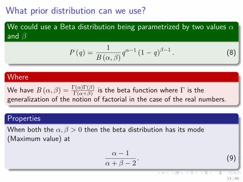
What prior distribution can we use?We could use a Beta distribution being parametrized by two values αand β

P (q) = 1B (α, β)qα−1 (1− q)β−1 . (8)

WhereWe have B (α, β) = Γ(α)Γ(β)

Γ(α+β) is the beta function where Γ is thegeneralization of the notion of factorial in the case of the real numbers.

PropertiesWhen both the α, β > 0 then the beta distribution has its mode(Maximum value) at

α− 1α+ β − 2 . (9)

13 / 66


P (q) = 1B (α, β)qα−1 (1− q)β−1 . (8)




α− 1α+ β − 2 . (9)

13 / 66


P (q) = 1B (α, β)qα−1 (1− q)β−1 . (8)




α− 1α+ β − 2 . (9)

13 / 66

We then do the following

We do the followingWe can choose α = β so the beta prior peaks at 0.5.

As a further expression of our beliefWe make the following choice α = β = 5.

Why? Look at the variance of the beta distributionαβ

(α+ β) (α+ β + 1) . (10)

14 / 66





(α+ β) (α+ β + 1) . (10)

14 / 66





(α+ β) (α+ β + 1) . (10)

14 / 66

Thus, we have the following nice properties

We have a variance with α = β = 5Var (q) ≈ 0.025

Thus, the standard deviationsd ≈ 0.16 which is a nice dispersion at the peak point!!!

15 / 66

Thus, we have the following nice properties

We have a variance with α = β = 5Var (q) ≈ 0.025

Thus, the standard deviationsd ≈ 0.16 which is a nice dispersion at the peak point!!!

15 / 66

Now, our MAP estimate for p...

We have then

p̂MAP = argmaxΘ

∑xi∈X

log p (xi |q) + log p (q)

(11)

Plugging back the ML

p̂MAP = argmaxΘ

[nPRI log q + (N − nPRI ) log (1− q) + log p (q)] (12)

Where

log P (p) = log( 1

B (α, β)qα−1 (1− q)β−1)

(13)

16 / 66


We have then

p̂MAP = argmaxΘ

∑xi∈X


(11)


p̂MAP = argmaxΘ


Where

log P (p) = log( 1

B (α, β)qα−1 (1− q)β−1)

(13)

16 / 66


We have then

p̂MAP = argmaxΘ

∑xi∈X


(11)


p̂MAP = argmaxΘ


Where

log P (p) = log( 1

B (α, β)qα−1 (1− q)β−1)

(13)

16 / 66

The log of P (p)

We have that

log P (q) = (α− 1) log q + (β − 1) log (1− q)− log B (α, β) (14)

Now taking the derivative with respect to p, we getnPRI

q − (N − nPRI )(1− q) − β − 1

1− q + α− 1q = 0 (15)

Thus

q̂MAP = nPRI + α− 1N + α+ β − 2 (16)

17 / 66

The log of P (p)

We have that



q − (N − nPRI )(1− q) − β − 1

1− q + α− 1q = 0 (15)

Thus

q̂MAP = nPRI + α− 1N + α+ β − 2 (16)

17 / 66

The log of P (p)

We have that



q − (N − nPRI )(1− q) − β − 1

1− q + α− 1q = 0 (15)

Thus

q̂MAP = nPRI + α− 1N + α+ β − 2 (16)

17 / 66

Now

With N = 20 with nPRI = 12 and α = β = 5

q̂MAP = 0.571

18 / 66

Outline



19 / 66

Properties

FirstMAP estimation “pulls” the estimate toward the prior.

SecondThe more focused our prior belief, the larger the pull toward the prior.

ExampleIf α = β=equal to large value

It will make the MAP estimate to move closer to the prior.

20 / 66

Properties





20 / 66

Properties





20 / 66

Properties

ThirdIn the expression we derived for q̂MAP , the parameters α and β play a“smoothing” role vis-a-vis the measurement nPRI .

FourthSince we referred to q as the parameter to be estimated, we can refer to αand β as the hyper-parameters in the estimation calculations.

21 / 66

Properties

ThirdIn the expression we derived for q̂MAP , the parameters α and β play a“smoothing” role vis-a-vis the measurement nPRI .

FourthSince we referred to q as the parameter to be estimated, we can refer to αand β as the hyper-parameters in the estimation calculations.

21 / 66

Beyond simple derivation

In the previous techniqueWe took an logarithm of the likelihoot × the prior to obtain a function thatcan be derived in order to obtain each of the parameters to be estimated.

What if we cannot derive?For example when we have something like |θi |.

We can try the followingEM + MAP to be able to estimate the sought parameters.

22 / 66





22 / 66





22 / 66

Outline



23 / 66

Example

This application comes from“Adaptive Sparseness for Supervised Learning” by Mário A.T. Figueiredo

InIEEE TRANSACTIONS ON PATTERN ANALYSIS AND MACHINEINTELLIGENCE, VOL. 25, NO. 9, SEPTEMBER 2003

24 / 66

Example

This application comes from“Adaptive Sparseness for Supervised Learning” by Mário A.T. Figueiredo

InIEEE TRANSACTIONS ON PATTERN ANALYSIS AND MACHINEINTELLIGENCE, VOL. 25, NO. 9, SEPTEMBER 2003

24 / 66

Outline



25 / 66

Introduction: Linear Regression with Gaussian Prior

We consider regression functions that are linear with respect to theparameter vector β

f (x, β) =k∑

i=1βih (x) = βT h (x)

Whereh (x) = [h1 (x) , ..., hk (x)]T is a vector of k fixed function of the input,often called features.

26 / 66

Introduction: Linear Regression with Gaussian Prior

We consider regression functions that are linear with respect to theparameter vector β

f (x, β) =k∑

i=1βih (x) = βT h (x)

Whereh (x) = [h1 (x) , ..., hk (x)]T is a vector of k fixed function of the input,often called features.

26 / 66

Actually, it can be...

Linear RegressionLinear regression, in which h (x) = [1, x1, ..., xd ]T i; in this case, k = d + 1.

Non-Linear RegressionHere, you have a fixed basis function whereh (x) = [φ1 (x) , φ2 (x) , ..., φ1 (x)]T with φ1 (x) = 1.

Kernel RegressionHere h (x) = [1,K (x,x1) ,K (x,x2) , ...,K (x,xn)]T where K (x,xi) issome kernel function.

27 / 66





27 / 66





27 / 66

Outline



28 / 66

Gaussian NoiseWe assume that the training set is contaminated by additive whiteGaussian Noise

yi = f (xi , β) + ωi (17)

for i = 1, ...,N where [ω1, ..., ωN ] is a set of independent zero-meanGaussian samples with variance σ2

Thus, for [y1, ..., yN ], we have the following likelihood

p (y|β) = N(Hβ, σ2I

)(18)

The posterior p (β|y) is still Gaussian and the mode is given by

β̂ =(σ2I + H T H

)−1H T y (19)

Remark: The Ridge regression.

29 / 66


yi = f (xi , β) + ωi (17)




)(18)


β̂ =(σ2I + H T H

)−1H T y (19)


29 / 66


yi = f (xi , β) + ωi (17)




)(18)


β̂ =(σ2I + H T H

)−1H T y (19)


29 / 66

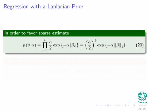
Regression with a Laplacian Prior

In order to favor sparse estimate

p (β|α) =k∏

i=1

α

2 exp {−α |βi |} =(α

2

)kexp {−α ‖β‖1} (20)

Thus, the MAP estimate of β look like

β̂ = argminβ

{‖Hβ − y‖22 + 2σ2α ‖β‖1

}(21)

30 / 66

Regression with a Laplacian Prior

In order to favor sparse estimate

p (β|α) =k∏

i=1

α

2 exp {−α |βi |} =(α

2

)kexp {−α ‖β‖1} (20)

Thus, the MAP estimate of β look like

β̂ = argminβ

{‖Hβ − y‖22 + 2σ2α ‖β‖1

}(21)

30 / 66

Remark

This criterion is know as the LASSOThis norm l1 induces sparsity in the weight terms.

How?For example,

∥∥∥[1, 0]T∥∥∥

2=∥∥∥[1/√2, 1/

√2]T∥∥∥

2= 1.

In the other case,∥∥∥[1, 0]T

∥∥∥1

= 1 <∥∥∥[1/√2, 1/

√2]T∥∥∥

2=√

2.

31 / 66

Remark


How?For example,

∥∥∥[1, 0]T∥∥∥

2=∥∥∥[1/√2, 1/

√2]T∥∥∥

2= 1.


∥∥∥1

= 1 <∥∥∥[1/√2, 1/

√2]T∥∥∥

2=√

2.

31 / 66

Remark


How?For example,

∥∥∥[1, 0]T∥∥∥

2=∥∥∥[1/√2, 1/

√2]T∥∥∥

2= 1.


∥∥∥1

= 1 <∥∥∥[1/√2, 1/

√2]T∥∥∥

2=√

2.

31 / 66

An example

What if H is a orthogonal matrixIn this case H T H = I

Thus

β̂ =argminβ

{‖Hβ − y‖22 + 2σ2α ‖β‖1

}=argmin

β

{(Hβ − y)T (Hβ − y) + 2σ2α

k∑i=1|βi |

}

=argminβ

{βT H T Hβ − 2βT H T y + yT y + 2σ2α

k∑i=1|βi |

}

=argminβ

{βTβ − 2βT H T y + yT y + 2σ2α

k∑i=1|βi |

}

32 / 66

An example


Thus

β̂ =argminβ

{‖Hβ − y‖22 + 2σ2α ‖β‖1

}=argmin

β

{(Hβ − y)T (Hβ − y) + 2σ2α

k∑i=1|βi |

}

=argminβ


k∑i=1|βi |

}

=argminβ


k∑i=1|βi |

}

32 / 66

An example


Thus

β̂ =argminβ

{‖Hβ − y‖22 + 2σ2α ‖β‖1

}=argmin

β

{(Hβ − y)T (Hβ − y) + 2σ2α

k∑i=1|βi |

}

=argminβ


k∑i=1|βi |

}

=argminβ


k∑i=1|βi |

}

32 / 66

An example


Thus

β̂ =argminβ

{‖Hβ − y‖22 + 2σ2α ‖β‖1

}=argmin

β

{(Hβ − y)T (Hβ − y) + 2σ2α

k∑i=1|βi |

}

=argminβ


k∑i=1|βi |

}

=argminβ


k∑i=1|βi |

}

32 / 66

An example


Thus

β̂ =argminβ

{‖Hβ − y‖22 + 2σ2α ‖β‖1

}=argmin

β

{(Hβ − y)T (Hβ − y) + 2σ2α

k∑i=1|βi |

}

=argminβ


k∑i=1|βi |

}

=argminβ


k∑i=1|βi |

}

32 / 66

We can solve this last part as follow

We can group for each βi

β2i − 2βi

(H T y

)i

+ 2σ2α |βi |+ y2i (22)

If we can minimize each group we will be able to get the solution

β̂i = argminβi

{β2

i − 2βi(H T y

)i

+ 2σ2α |βi |}

(23)

We have two casesβi > 0βi < 0

33 / 66



β2i − 2βi

(H T y

)i

+ 2σ2α |βi |+ y2i (22)


β̂i = argminβi

{β2

i − 2βi(H T y

)i

+ 2σ2α |βi |}

(23)


33 / 66



β2i − 2βi

(H T y

)i

+ 2σ2α |βi |+ y2i (22)


β̂i = argminβi

{β2

i − 2βi(H T y

)i

+ 2σ2α |βi |}

(23)


33 / 66



β2i − 2βi

(H T y

)i

+ 2σ2α |βi |+ y2i (22)


β̂i = argminβi

{β2

i − 2βi(H T y

)i

+ 2σ2α |βi |}

(23)


33 / 66

If βi > 0

We then derive with respect to βi

∂(β2

i − 2βi(H T y

)i

+ 2σ2αiβi)

∂βi= 2βi − 2

(H T y

)i

+ 2σ2α

We have then

β̂i =(H T y

)i− σ2α (24)

34 / 66

If βi > 0


∂(β2

i − 2βi(H T y

)i

+ 2σ2αiβi)

∂βi= 2βi − 2

(H T y

)i

+ 2σ2α

We have then

β̂i =(H T y

)i− σ2α (24)

34 / 66

If βi < 0


∂(β2

i − 2βi(H T y

)i− 2σ2αiβi

)∂βi

= 2βi − 2(H T y

)i− 2σ2α

We have then

β̂i =(H T y

)i

+ σ2α (25)

35 / 66

If βi < 0


∂(β2

i − 2βi(H T y

)i− 2σ2αiβi

)∂βi

= 2βi − 2(H T y

)i− 2σ2α

We have then

β̂i =(H T y

)i

+ σ2α (25)

35 / 66

The value of(H Ty

)i

Ww have thatWe have that:

if βi > 0 then(H T y

)i> σ2α

if βi < 0 then(H T y

)i< −σ2α

36 / 66

We can put all this together

A compact Version

β̂i = sgn((

H T y)

i

) (∣∣∣(H T y)

i

∣∣∣− σ2α)

+(26)

With

(a)+ ={

a if a ≥ 00 if a < 0

and “sgn” is the sign function.

This rule is know as theThe soft threshold!!!

37 / 66


A compact Version

β̂i = sgn((

H T y)

i

) (∣∣∣(H T y)

i

∣∣∣− σ2α)

+(26)

With

(a)+ ={

a if a ≥ 00 if a < 0



37 / 66


A compact Version

β̂i = sgn((

H T y)

i

) (∣∣∣(H T y)

i

∣∣∣− σ2α)

+(26)

With

(a)+ ={

a if a ≥ 00 if a < 0



37 / 66

Example

We have the doted · · · line as the soft threshold

a

3

2

1

0

-1

-2

-3

-3 -2 -1 0 1 2 3

38 / 66

Outline



39 / 66

Now

Given that each βi has a zero-mean Gaussian prior

p (βi |τi) = N (βi |0, τi) (27)

Where τi has the following exponential hyperprior

p (τi |γ) = γ

2 exp{−γ2 τi

}for τi ≥ 0 (28)

This is a though property - so we take it by heart

p (βi |γ) =ˆ ∞

0p (βi |τi) p (τi |γ) dτi =

√γ

2 exp {−√γ |βi |} (29)

40 / 66

Now


p (βi |τi) = N (βi |0, τi) (27)


p (τi |γ) = γ

2 exp{−γ2 τi

}for τi ≥ 0 (28)


p (βi |γ) =ˆ ∞


√γ

2 exp {−√γ |βi |} (29)

40 / 66

Now


p (βi |τi) = N (βi |0, τi) (27)


p (τi |γ) = γ

2 exp{−γ2 τi

}for τi ≥ 0 (28)


p (βi |γ) =ˆ ∞


√γ

2 exp {−√γ |βi |} (29)

40 / 66

Example

The double exponential

41 / 66

This is equivalent to the use of the L1-norm forregularization

L1(Left) is better for sparsity promotion than L2(Right)

42 / 66

Outline



43 / 66

The EM trick

How do we do this?This is done by regarding τ = [τ1, ..., τk ] as the hidden/missing data

Then, if we could observe τ , complete log-posterior log p (β, σ2|y, τ)can be easily calculated

p(β, σ2|y, τ

)∝ p

(y|β, σ2

)p (β|τ) p

(σ2)

(30)

Wherep(y|β, σ2) ∼ N (β, σ2)

p (β|0, τ) ∼ N (0, τ)

44 / 66

The EM trick



p(β, σ2|y, τ

)∝ p

(y|β, σ2

)p (β|τ) p

(σ2)

(30)


p (β|0, τ) ∼ N (0, τ)

44 / 66

The EM trick



p(β, σ2|y, τ

)∝ p

(y|β, σ2

)p (β|τ) p

(σ2)

(30)


p (β|0, τ) ∼ N (0, τ)

44 / 66

What about p (σ2)?

We selectp(σ2) as a constant

HoweverWe can adopt a conjugate inverse Gamma prior for σ2, but for largenumber of samples the prior on the estimate of σ2is very small.

In the constant caseWe can use the MAP idea, however we have hidden parameters so weresort to the EM

45 / 66

What about p (σ2)?




45 / 66

What about p (σ2)?




45 / 66

E-step

Computes the expected value of the complete log-posterior

Q(β, σ2|β̂(t), σ̂2(t)

)=ˆ

log p(β, σ2|y, τ

)p(τ |β̂(t), σ̂2(t),y

)dτ (31)

46 / 66

M-step

Updates the parameter estimates by maximizing the Q-function(β̂(t+1), σ̂2(t+1)

)= argmax

β,σ2Q(β, σ2|β̂(t), σ̂2(t)

)(32)

47 / 66

Remark

FirstThe EM algorithm converges to a local maximum of the a posterioriprobability density function

p(β, σ2|y

)∝ p

(y|β, σ2

)p (β|γ) (33)

Without using the marginal prior p (β|γ) which is not GaussianInstead we use a conditional Gaussian prior p (β|γ)

48 / 66

Remark

FirstThe EM algorithm converges to a local maximum of the a posterioriprobability density function

p(β, σ2|y

)∝ p

(y|β, σ2

)p (β|γ) (33)

Without using the marginal prior p (β|γ) which is not GaussianInstead we use a conditional Gaussian prior p (β|γ)

48 / 66

The Final Model

We have

p(y|β, σ2

)= N

(Hβ, σ2I

)p(σ2)∝ ”constant”

p (β|τ) =k∏

i=1N (βi |0, τi) = N

(β|0, (Υ (τ))−1

)

p (τ |γ) =(γ

2

)k k∏i=1

exp{−γ2 τi

}

With Υ (τ) = diag(τ−1

1 , ..., τ−1k

)is the diagonal matrix with the inverse

variances of all the βi ’s.

49 / 66

The Final Model

We have

p(y|β, σ2

)= N

(Hβ, σ2I


p (β|τ) =k∏

i=1N (βi |0, τi) = N

(β|0, (Υ (τ))−1

)

p (τ |γ) =(γ

2

)k k∏i=1

exp{−γ2 τi

}


1 , ..., τ−1k



49 / 66

The Final Model

We have

p(y|β, σ2

)= N

(Hβ, σ2I


p (β|τ) =k∏

i=1N (βi |0, τi) = N

(β|0, (Υ (τ))−1

)

p (τ |γ) =(γ

2

)k k∏i=1

exp{−γ2 τi

}


1 , ..., τ−1k



49 / 66

The Final Model

We have

p(y|β, σ2

)= N

(Hβ, σ2I


p (β|τ) =k∏

i=1N (βi |0, τi) = N

(β|0, (Υ (τ))−1

)

p (τ |γ) =(γ

2

)k k∏i=1

exp{−γ2 τi

}


1 , ..., τ−1k



49 / 66

The Final Model

We have

p(y|β, σ2

)= N

(Hβ, σ2I


p (β|τ) =k∏

i=1N (βi |0, τi) = N

(β|0, (Υ (τ))−1

)

p (τ |γ) =(γ

2

)k k∏i=1

exp{−γ2 τi

}


1 , ..., τ−1k



49 / 66

Now, we find the Q function

First

log p(β, σ2|y, τ

)∝ log p

(y|β, σ2

)+ log p (β|τ)

∝ −n log σ2 − ‖y −Hβ‖22σ2 − βTΥ (τ)β

How can we get this?Remember

N (y|µ,Σ) = 1(2π)

k2 |Σ|

12

exp{−1

2 (y − µ)T Σ−1}

(34)

Volunteers?Please to the blackboard.

50 / 66


First

log p(β, σ2|y, τ

)∝ log p

(y|β, σ2

)+ log p (β|τ)

∝ −n log σ2 − ‖y −Hβ‖22σ2 − βTΥ (τ)β


N (y|µ,Σ) = 1(2π)

k2 |Σ|

12

exp{−1

2 (y − µ)T Σ−1}

(34)


50 / 66


First

log p(β, σ2|y, τ

)∝ log p

(y|β, σ2

)+ log p (β|τ)

∝ −n log σ2 − ‖y −Hβ‖22σ2 − βTΥ (τ)β


N (y|µ,Σ) = 1(2π)

k2 |Σ|

12

exp{−1

2 (y − µ)T Σ−1}

(34)


50 / 66

Thus

SecondDid you notice that the term βTΥ (τ)β is linear with respect to Υ (τ) andthe other terms do not depend on τ?

Thus, the E-step is reduced to the computation of Υ (τ)

V (t) = E(Υ (τ) |y, β̂(t), σ̂2(t)

)= diag

(E[τ−1

1 |y, β̂(t), σ̂2(t)], ...,E

[τ−1

k |y, β̂(t), σ̂2(t)])

51 / 66

Thus



V (t) = E(Υ (τ) |y, β̂(t), σ̂2(t)

)= diag

(E[τ−1

1 |y, β̂(t), σ̂2(t)], ...,E

[τ−1

k |y, β̂(t), σ̂2(t)])

51 / 66

Thus



V (t) = E(Υ (τ) |y, β̂(t), σ̂2(t)

)= diag

(E[τ−1

1 |y, β̂(t), σ̂2(t)], ...,E

[τ−1

k |y, β̂(t), σ̂2(t)])

51 / 66

Now

What do we need to calculate each of this expectations?

p(τi |y, β̂(t), σ̂2(t)

)= p

(τi |y, β̂i,(t), σ̂2i,(t)

)(35)

Then

p(τi |y, β̂i,(t), σ̂2i,(t)

)=

p(τi , β̂i,(t)|y, σ̂2i,(t)

)p(β̂i,(t)|y, σ̂2i,(t)

)∝ p

(β̂i,(t)|τi ,y, σ̂2i,(t)

)p(τi |y, σ̂2i,(t)

)= p

(β̂i,(t)|τi

)p (τi)

52 / 66

Now


p(τi |y, β̂(t), σ̂2(t)

)= p

(τi |y, β̂i,(t), σ̂2i,(t)

)(35)

Then

p(τi |y, β̂i,(t), σ̂2i,(t)

)=

p(τi , β̂i,(t)|y, σ̂2i,(t)

)p(β̂i,(t)|y, σ̂2i,(t)

)∝ p

(β̂i,(t)|τi ,y, σ̂2i,(t)

)p(τi |y, σ̂2i,(t)

)= p

(β̂i,(t)|τi

)p (τi)

52 / 66

Now


p(τi |y, β̂(t), σ̂2(t)

)= p

(τi |y, β̂i,(t), σ̂2i,(t)

)(35)

Then

p(τi |y, β̂i,(t), σ̂2i,(t)

)=

p(τi , β̂i,(t)|y, σ̂2i,(t)

)p(β̂i,(t)|y, σ̂2i,(t)

)∝ p

(β̂i,(t)|τi ,y, σ̂2i,(t)

)p(τi |y, σ̂2i,(t)

)= p

(β̂i,(t)|τi

)p (τi)

52 / 66

Now


p(τi |y, β̂(t), σ̂2(t)

)= p

(τi |y, β̂i,(t), σ̂2i,(t)

)(35)

Then

p(τi |y, β̂i,(t), σ̂2i,(t)

)=

p(τi , β̂i,(t)|y, σ̂2i,(t)

)p(β̂i,(t)|y, σ̂2i,(t)

)∝ p

(β̂i,(t)|τi ,y, σ̂2i,(t)

)p(τi |y, σ̂2i,(t)

)= p

(β̂i,(t)|τi

)p (τi)

52 / 66

Here is the interesting part

We have the following probability density

p(τi |y, β̂i,(t), σ̂2i,(t)

)=

N(βi,(t)|0, τi

)γ2 exp

{−γ

2 τi}

´∞0 N

(βi,(t)|0, τi

)γ2 exp

{−γ

2 τi}

dτi(36)

Then

E[τ−1

1 |y, β̂i,(t), σ̂2(t)]

=

´∞0

1τiN(βi,(t)|0, τi

)γ2 exp

{−γ

2 τi}

dτi´∞0 N

(βi,(t)|0, τi

)γ2 exp

{−γ

2 τi}

dτi(37)

NowI leave to you to prove that (It can come in the test)

53 / 66



p(τi |y, β̂i,(t), σ̂2i,(t)

)=

N(βi,(t)|0, τi

)γ2 exp

{−γ

2 τi}

´∞0 N

(βi,(t)|0, τi

)γ2 exp

{−γ

2 τi}

dτi(36)

Then

E[τ−1

1 |y, β̂i,(t), σ̂2(t)]

=

´∞0


)γ2 exp

{−γ

2 τi}

dτi´∞0 N

(βi,(t)|0, τi

)γ2 exp

{−γ

2 τi}

dτi(37)


53 / 66



p(τi |y, β̂i,(t), σ̂2i,(t)

)=

N(βi,(t)|0, τi

)γ2 exp

{−γ

2 τi}

´∞0 N

(βi,(t)|0, τi

)γ2 exp

{−γ

2 τi}

dτi(36)

Then

E[τ−1

1 |y, β̂i,(t), σ̂2(t)]

=

´∞0


)γ2 exp

{−γ

2 τi}

dτi´∞0 N

(βi,(t)|0, τi

)γ2 exp

{−γ

2 τi}

dτi(37)


53 / 66


Thus

E[τ−1

1 |y, β̂i,(t), σ̂2(t)]

= γ∣∣∣β̂i,(t)

∣∣∣ (38)

Finally

V (t) = γdiag(∣∣∣β̂1,(t)

∣∣∣−1, ...,

∣∣∣β̂k,(t)

∣∣∣−1)

(39)

54 / 66


Thus

E[τ−1

1 |y, β̂i,(t), σ̂2(t)]

= γ∣∣∣β̂i,(t)

∣∣∣ (38)

Finally

V (t) = γdiag(∣∣∣β̂1,(t)

∣∣∣−1, ...,

∣∣∣β̂k,(t)

∣∣∣−1)

(39)

54 / 66

The Final Q function

Something Notable

Q(β, σ2|β̂(t), σ̂2(t)

)=ˆ

log p(β, σ2|y, τ

)p(τ |β̂(t), σ̂2(t), y

)dτ

=ˆ [−n log σ2 −

‖y −Hβ‖22

σ2 − βTΥ (τ)β]

p(τ |β̂(t), σ̂2(t), y

)dτ

= −n log σ2 −‖y −Hβ‖2

2σ2 − βT

[ˆΥ (τ) p

(τ |β̂(t), σ̂2(t), y

)dτ]β

= −n log σ2 −‖y −Hβ‖2

2σ2 − βT V (t)β

55 / 66


Something Notable

Q(β, σ2|β̂(t), σ̂2(t)

)=ˆ

log p(β, σ2|y, τ

)p(τ |β̂(t), σ̂2(t), y

)dτ


‖y −Hβ‖22


p(τ |β̂(t), σ̂2(t), y

)dτ

= −n log σ2 −‖y −Hβ‖2

2σ2 − βT

[ˆΥ (τ) p

(τ |β̂(t), σ̂2(t), y

)dτ]β

= −n log σ2 −‖y −Hβ‖2


55 / 66


Something Notable

Q(β, σ2|β̂(t), σ̂2(t)

)=ˆ

log p(β, σ2|y, τ

)p(τ |β̂(t), σ̂2(t), y

)dτ


‖y −Hβ‖22


p(τ |β̂(t), σ̂2(t), y

)dτ

= −n log σ2 −‖y −Hβ‖2

2σ2 − βT

[ˆΥ (τ) p

(τ |β̂(t), σ̂2(t), y

)dτ]β

= −n log σ2 −‖y −Hβ‖2


55 / 66


Something Notable

Q(β, σ2|β̂(t), σ̂2(t)

)=ˆ

log p(β, σ2|y, τ

)p(τ |β̂(t), σ̂2(t), y

)dτ


‖y −Hβ‖22


p(τ |β̂(t), σ̂2(t), y

)dτ

= −n log σ2 −‖y −Hβ‖2

2σ2 − βT

[ˆΥ (τ) p

(τ |β̂(t), σ̂2(t), y

)dτ]β

= −n log σ2 −‖y −Hβ‖2


55 / 66

Finally, the M-stepFirst

σ̂2(t+1) = argmaxσ2

{−n log σ2 − ‖y −Hβ‖22

σ2

}

= ‖y −Hβ‖22n

Second

β̂(t+1) = argmaxβ

{−‖y −Hβ‖22

σ2 − βT V (t)β

}

=(σ̂2(t+1)V (t) + H T H

)−1H T y

This also I leave to youIt can come in the test.

56 / 66



{−n log σ2 − ‖y −Hβ‖22

σ2

}

= ‖y −Hβ‖22n

Second


{−‖y −Hβ‖22

σ2 − βT V (t)β

}

=(σ̂2(t+1)V (t) + H T H

)−1H T y


56 / 66



{−n log σ2 − ‖y −Hβ‖22

σ2

}

= ‖y −Hβ‖22n

Second


{−‖y −Hβ‖22

σ2 − βT V (t)β

}

=(σ̂2(t+1)V (t) + H T H

)−1H T y


56 / 66



{−n log σ2 − ‖y −Hβ‖22

σ2

}

= ‖y −Hβ‖22n

Second


{−‖y −Hβ‖22

σ2 − βT V (t)β

}

=(σ̂2(t+1)V (t) + H T H

)−1H T y


56 / 66



{−n log σ2 − ‖y −Hβ‖22

σ2

}

= ‖y −Hβ‖22n

Second


{−‖y −Hβ‖22

σ2 − βT V (t)β

}

=(σ̂2(t+1)V (t) + H T H

)−1H T y


56 / 66

Outline



57 / 66

However

We need to deal in some way with the γ termIt controls the degree of spareness!!!

We can do assuming a Jeffrey’s PriorJ. Berger, Statistical Decision Theory and Bayesian Analysis. New York:Springer-Verlag, 1980.

We use instead

p (τ) ∝ 1τ

(40)

58 / 66

However



We use instead

p (τ) ∝ 1τ

(40)

58 / 66

However



We use instead

p (τ) ∝ 1τ

(40)

58 / 66

Properties of the Jeffrey’s Prior

ImportantThis prior expresses ignorance with respect to scale and is parameter free

Why scale invariantImagine, we change the scale of τ by τ ′ = Kτ where K is a constantexpressing that change

Thus, we have that

p(τ ′)

= 1τ ′

= 1kτ ∝

1τ

(41)

59 / 66




Thus, we have that

p(τ ′)

= 1τ ′

= 1kτ ∝

1τ

(41)

59 / 66




Thus, we have that

p(τ ′)

= 1τ ′

= 1kτ ∝

1τ

(41)

59 / 66

However

Something NotableThis prior is known as an improper prior.

In additionThis prior does not leads to a Laplacian prior on β.

NeverthelessThis prior induces sparseness and good performance for the β.

60 / 66

However




60 / 66

However




60 / 66

Introducing this prior into the equations

Matrix V (t) is now

V (t) = diag(∣∣∣β̂1,(t)

∣∣∣−2, ...,

∣∣∣β̂k,(t)

∣∣∣−2)

(42)

Quite interesting!!!We do not have the free γ parameter.

61 / 66

Introducing this prior into the equations

Matrix V (t) is now

V (t) = diag(∣∣∣β̂1,(t)

∣∣∣−2, ...,

∣∣∣β̂k,(t)

∣∣∣−2)

(42)

Quite interesting!!!We do not have the free γ parameter.

61 / 66

Here, we can see the new thresholdWith dotted line as the soft threshold, dashed the hard threshold andin blue solid the Jeffrey’s prior

a

3

2

1

0

-1

-2

-3

-3 -2 -1 0 1 2 3

62 / 66

Observations

The new rule is betweenThe soft threshold rule.The hard threshold rule.

Something NotableWith large values of

(H T y

)ithe new rule approaches the hard threshold.

Once(H Ty

)igets smaller

The estimate becomes progressively smaller approaching the behavior ofthe soft rule.

63 / 66

Observations



(H T y


Once(H Ty

)igets smaller


63 / 66

Observations



(H T y


Once(H Ty

)igets smaller


63 / 66

Finally, an implementation detail

Since several elements of β̂ will go to zero

V (t) = diag(∣∣∣β̂1,(t)

∣∣∣−2, ...,

∣∣∣β̂k,(t)

∣∣∣−2)

will have several elements going tolarge numbers

Something Notableif we define U (t) = diag

(∣∣∣β̂1,(t)

∣∣∣ , ..., ∣∣∣β̂k,(t)

∣∣∣).Then, we have that

V (t) = U−1(t) U−1

(t) (43)

64 / 66



V (t) = diag(∣∣∣β̂1,(t)

∣∣∣−2, ...,

∣∣∣β̂k,(t)

∣∣∣−2)



(∣∣∣β̂1,(t)

∣∣∣ , ..., ∣∣∣β̂k,(t)


V (t) = U−1(t) U−1

(t) (43)

64 / 66



V (t) = diag(∣∣∣β̂1,(t)

∣∣∣−2, ...,

∣∣∣β̂k,(t)

∣∣∣−2)



(∣∣∣β̂1,(t)

∣∣∣ , ..., ∣∣∣β̂k,(t)


V (t) = U−1(t) U−1

(t) (43)

64 / 66

Thus

We have that

β̂(t+1) =(σ̂2(t+1)V (t) + H T H

)−1H T y

=(σ̂2(t+1)U−1

(t) U−1(t) + H T H

)−1H T y

=(σ̂2(t+1)U−1

(t) I U−1(t) + I H T H I

)−1H T y

=(σ̂2(t+1)U−1

(t) I U−1(t) + U−1

(t) U (t)H T HU (t)U−1(t)

)−1H T y

= U (t)(σ̂2(t+1)I + U (t)H T HU (t)

)−1U (t)H T y

65 / 66

Thus

We have that

β̂(t+1) =(σ̂2(t+1)V (t) + H T H

)−1H T y

=(σ̂2(t+1)U−1

(t) U−1(t) + H T H

)−1H T y

=(σ̂2(t+1)U−1

(t) I U−1(t) + I H T H I

)−1H T y

=(σ̂2(t+1)U−1

(t) I U−1(t) + U−1


)−1H T y

= U (t)(σ̂2(t+1)I + U (t)H T HU (t)

)−1U (t)H T y

65 / 66

Thus

We have that

β̂(t+1) =(σ̂2(t+1)V (t) + H T H

)−1H T y

=(σ̂2(t+1)U−1

(t) U−1(t) + H T H

)−1H T y

=(σ̂2(t+1)U−1

(t) I U−1(t) + I H T H I

)−1H T y

=(σ̂2(t+1)U−1

(t) I U−1(t) + U−1


)−1H T y

= U (t)(σ̂2(t+1)I + U (t)H T HU (t)

)−1U (t)H T y

65 / 66

Thus

We have that

β̂(t+1) =(σ̂2(t+1)V (t) + H T H

)−1H T y

=(σ̂2(t+1)U−1

(t) U−1(t) + H T H

)−1H T y

=(σ̂2(t+1)U−1

(t) I U−1(t) + I H T H I

)−1H T y

=(σ̂2(t+1)U−1

(t) I U−1(t) + U−1


)−1H T y

= U (t)(σ̂2(t+1)I + U (t)H T HU (t)

)−1U (t)H T y

65 / 66

Thus

We have that

β̂(t+1) =(σ̂2(t+1)V (t) + H T H

)−1H T y

=(σ̂2(t+1)U−1

(t) U−1(t) + H T H

)−1H T y

=(σ̂2(t+1)U−1

(t) I U−1(t) + I H T H I

)−1H T y

=(σ̂2(t+1)U−1

(t) I U−1(t) + U−1


)−1H T y

= U (t)(σ̂2(t+1)I + U (t)H T HU (t)

)−1U (t)H T y

65 / 66

Advantages!!!

Quite ImportantWe avoid the inversion of the elements of β̂(t).

We can avoid getting the inverse matrixWe simply solve the corresponding linear system whose dimension is onlythe number of nonzero elements in U (t). Why?

Remember you want to maximizeQ(β, σ2|β̂(t), σ̂2(t)

)= −n log σ2 − ‖y−Hβ‖2


66 / 66

Advantages!!!




)= −n log σ2 − ‖y−Hβ‖2


66 / 66

Advantages!!!




)= −n log σ2 − ‖y−Hβ‖2


66 / 66

Engineering

08 Machine Learning Maximum Aposteriori