Embed Size (px)
Citation preview

Introduction Sparse FHT algorithm Analysis of probability of failure Empirical results Conclusion
A Fast Hadamard Transform for Signals withSub-linear Sparsity
Robin Scheibler Saeid Haghighatshoar Martin Vetterli
School of Computer and Communication SciencesÉcole Polytechnique Fédérale de Lausanne, Switzerland
October 28, 2013
SparseFHT 1 / 20 EPFL

Introduction Sparse FHT algorithm Analysis of probability of failure Empirical results Conclusion
Why the Hadamard transform ?
I Historically, low computationapproximation to DFT.
I Coding, 1969 Mariner Mars probe.
I Communication, orthogonal codesin WCDMA.
I Compressed sensing, maximallyincoherent with Dirac basis.
I Spectroscopy, design ofinstruments with lower noise.
I Recent advances in sparse FFT.
16 ⇥ 16 Hadamard matrix
Mariner probe
SparseFHT 2 / 20 EPFL
Introduction Sparse FHT algorithm Analysis of probability of failure Empirical results Conclusion
Fast Hadamard transform
I Butterfly structure similar to FFT.I Time complexity O(N log2 N).I Sample complexity N.+ Universal, i.e. works for all signals.� Does not exploit signal structure
(e.g. sparsity).
Can we do better ?
SparseFHT 3 / 20 EPFL

Introduction Sparse FHT algorithm Analysis of probability of failure Empirical results Conclusion
Contribution: Sparse fast Hadamard transform
Assumptions
I The signal is exaclty K -sparse in the transform domain.I Sub-linear sparsity regime K = O(N↵), 0 < ↵ < 1.I Support of the signal is uniformly random.
ContributionAn algorithm computing the K non-zero coefficients with:
I Time complexity O(K log2 K log2NK ).
I Sample complexity O(K log2NK ).
I Probability of failure asymptotically vanishes.
SparseFHT 4 / 20 EPFL
Introduction Sparse FHT algorithm Analysis of probability of failure Empirical results Conclusion
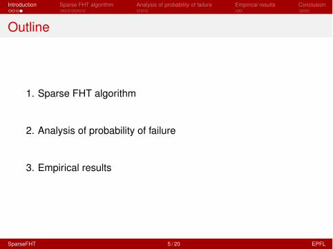
Outline
1. Sparse FHT algorithm
2. Analysis of probability of failure
3. Empirical results
SparseFHT 5 / 20 EPFL

Introduction Sparse FHT algorithm Analysis of probability of failure Empirical results Conclusion
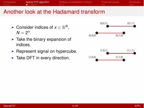
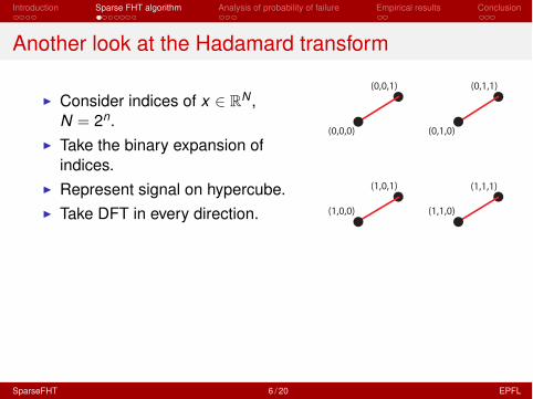
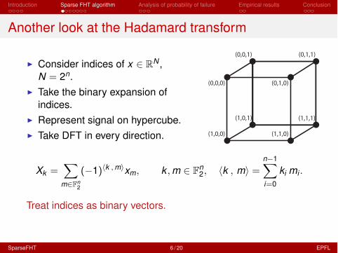
Another look at the Hadamard transform
I Consider indices of x 2 RN ,N = 2n.
I Take the binary expansion ofindices.
I Represent signal on hypercube.I Take DFT in every direction.
I = {0, . . . , 23 � 1}
SparseFHT 6 / 20 EPFL

Introduction Sparse FHT algorithm Analysis of probability of failure Empirical results Conclusion
Another look at the Hadamard transform
I Consider indices of x 2 RN ,N = 2n.
I Take the binary expansion ofindices.
I Represent signal on hypercube.I Take DFT in every direction.
I = {(0, 0, 0), . . . , (1, 1, 1)}
SparseFHT 6 / 20 EPFL

Introduction Sparse FHT algorithm Analysis of probability of failure Empirical results Conclusion
Another look at the Hadamard transform
I Consider indices of x 2 RN ,N = 2n.
I Take the binary expansion ofindices.
I Represent signal on hypercube.I Take DFT in every direction.
(0,0,0) (0,1,0)
(1,0,1) (1,1,1)
(1,1,0)(1,0,0)
(0,0,1) (0,1,1)
SparseFHT 6 / 20 EPFL

Introduction Sparse FHT algorithm Analysis of probability of failure Empirical results Conclusion
Another look at the Hadamard transform
I Consider indices of x 2 RN ,N = 2n.
I Take the binary expansion ofindices.
I Represent signal on hypercube.I Take DFT in every direction.
(0,0,0) (0,1,0)
(1,0,1) (1,1,1)
(1,1,0)(1,0,0)
(0,0,1) (0,1,1)
Xk0,...,kn�1 =1X
m0=0
· · ·1X
mn�1=0
(�1)k0m0+···+kn�1mn�1xm0,...,mn�1 ,
SparseFHT 6 / 20 EPFL

Introduction Sparse FHT algorithm Analysis of probability of failure Empirical results Conclusion
Another look at the Hadamard transform
I Consider indices of x 2 RN ,N = 2n.
I Take the binary expansion ofindices.
I Represent signal on hypercube.I Take DFT in every direction.
(0,0,0) (0,1,0)
(1,0,1) (1,1,1)
(1,1,0)(1,0,0)
(0,0,1) (0,1,1)
Xk =X
m2Fn2
(�1)hk ,mixm, k ,m 2 Fn2, hk , mi =
n�1X
i=0
ki mi .
Treat indices as binary vectors.
SparseFHT 6 / 20 EPFL

Introduction Sparse FHT algorithm Analysis of probability of failure Empirical results Conclusion
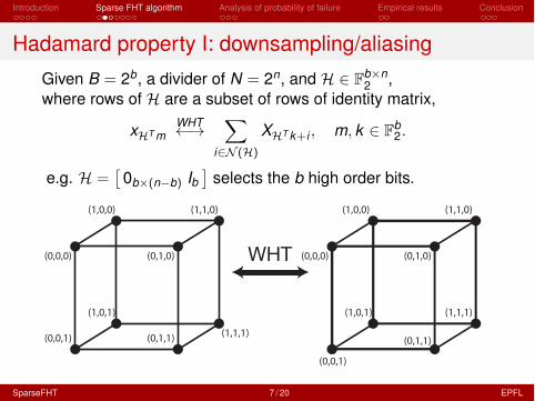
Hadamard property I: downsampling/aliasingGiven B = 2b, a divider of N = 2n, and H 2 Fb⇥n
2 ,where rows of H are a subset of rows of identity matrix,
xHT mWHT !
X
i2N (H)
XHT k+i , m, k 2 Fb2.
e.g. H =⇥
0b⇥(n�b) Ib⇤
selects the b high order bits.
SparseFHT 7 / 20 EPFL

Introduction Sparse FHT algorithm Analysis of probability of failure Empirical results Conclusion
Hadamard property I: downsampling/aliasingGiven B = 2b, a divider of N = 2n, and H 2 Fb⇥n
2 ,where rows of H are a subset of rows of identity matrix,
xHT mWHT !
X
i2N (H)
XHT k+i , m, k 2 Fb2.
e.g. H =⇥
0b⇥(n�b) Ib⇤
selects the b high order bits.
SparseFHT 7 / 20 EPFL
Introduction Sparse FHT algorithm Analysis of probability of failure Empirical results Conclusion
Hadamard property I: downsampling/aliasingGiven B = 2b, a divider of N = 2n, and H 2 Fb⇥n
2 ,where rows of H are a subset of rows of identity matrix,
xHT mWHT !
X
i2N (H)
XHT k+i , m, k 2 Fb2.
e.g. H =⇥
0b⇥(n�b) Ib⇤
selects the b high order bits.
(0,0,0) (0,1,0)
(1,0,1)
(1,1,1)(0,1,1)(0,0,1)
(1,0,0) (1,1,0)
(0,0,0) (0,1,0)
(1,0,1) (1,1,1)
(0,1,1)
(0,0,1)
(1,0,0) (1,1,0)
WHT
SparseFHT 7 / 20 EPFL
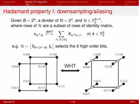
Introduction Sparse FHT algorithm Analysis of probability of failure Empirical results Conclusion
Hadamard property I: downsampling/aliasingGiven B = 2b, a divider of N = 2n, and H 2 Fb⇥n
2 ,where rows of H are a subset of rows of identity matrix,
xHT mWHT !
X
i2N (H)
XHT k+i , m, k 2 Fb2.
e.g. H =⇥
0b⇥(n�b) Ib⇤
selects the b high order bits.
(0,0,0) (0,1,0)
(0,1,1)(0,0,1)
(0,0,0) (0,1,0)
(1,0,1) (1,1,1)
(0,1,1)(0,0,1)
(1,0,0) (1,1,0)
(1,0,1)
(1,1,1)
(1,0,0) (1,1,0)
WHT
SparseFHT 7 / 20 EPFL

Introduction Sparse FHT algorithm Analysis of probability of failure Empirical results Conclusion
Aliasing induced bipartite graph
time-domain
Hadamard-domain
I Downsampling induces an aliasing pattern.I Different downsamplings produce different patterns.
SparseFHT 8 / 20 EPFL

Introduction Sparse FHT algorithm Analysis of probability of failure Empirical results Conclusion
Aliasing induced bipartite graph
time-domain
Hadamard-domain
4-WHT
I Downsampling induces an aliasing pattern.I Different downsamplings produce different patterns.
SparseFHT 8 / 20 EPFL

Introduction Sparse FHT algorithm Analysis of probability of failure Empirical results Conclusion
Aliasing induced bipartite graph
time-domain
Hadamard-domain
4-WHT
I Downsampling induces an aliasing pattern.I Different downsamplings produce different patterns.
SparseFHT 8 / 20 EPFL

Introduction Sparse FHT algorithm Analysis of probability of failure Empirical results Conclusion
Aliasing induced bipartite graph
time-domain
Hadamard-domain
4-WHT 4-WHT
I Downsampling induces an aliasing pattern.I Different downsamplings produce different patterns.
SparseFHT 8 / 20 EPFL

Introduction Sparse FHT algorithm Analysis of probability of failure Empirical results Conclusion
Aliasing induced bipartite graph
time-domain
Hadamard-domain
4-WHT 4-WHT
I Downsampling induces an aliasing pattern.I Different downsamplings produce different patterns.
SparseFHT 8 / 20 EPFL

Introduction Sparse FHT algorithm Analysis of probability of failure Empirical results Conclusion
Aliasing induced bipartite graph
time-domain
Hadamard-domain
4-WHT 4-WHT
Checks
Variables
I Downsampling induces an aliasing pattern.I Different downsamplings produce different patterns.
SparseFHT 8 / 20 EPFL

Introduction Sparse FHT algorithm Analysis of probability of failure Empirical results Conclusion
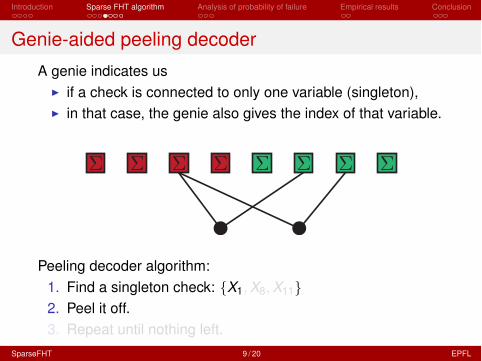
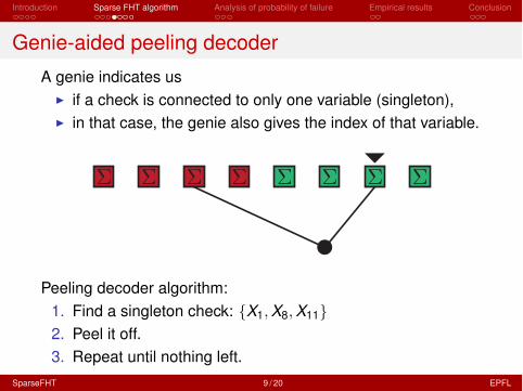
Genie-aided peeling decoderA genie indicates us
I if a check is connected to only one variable (singleton),I in that case, the genie also gives the index of that variable.
Peeling decoder algorithm:1. Find a singleton check: {X1,X8,X11}2. Peel it off.3. Repeat until nothing left.
SparseFHT 9 / 20 EPFL

Introduction Sparse FHT algorithm Analysis of probability of failure Empirical results Conclusion
Genie-aided peeling decoderA genie indicates us
I if a check is connected to only one variable (singleton),I in that case, the genie also gives the index of that variable.
Peeling decoder algorithm:1. Find a singleton check: {X1,X8,X11}2. Peel it off.3. Repeat until nothing left.
SparseFHT 9 / 20 EPFL

Introduction Sparse FHT algorithm Analysis of probability of failure Empirical results Conclusion
Genie-aided peeling decoderA genie indicates us
I if a check is connected to only one variable (singleton),I in that case, the genie also gives the index of that variable.
SuccessPeeling decoder algorithm:
1. Find a singleton check: {X1,X8,X11}2. Peel it off.3. Repeat until nothing left.
SparseFHT 9 / 20 EPFL

Introduction Sparse FHT algorithm Analysis of probability of failure Empirical results Conclusion
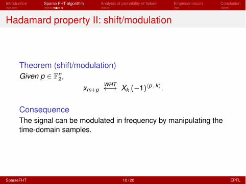
Hadamard property II: shift/modulation
Theorem (shift/modulation)Given p 2 Fn
2,xm+p
WHT ! Xk (�1)hp , ki.
ConsequenceThe signal can be modulated in frequency by manipulating thetime-domain samples.
SparseFHT 10 / 20 EPFL
Introduction Sparse FHT algorithm Analysis of probability of failure Empirical results Conclusion
Hadamard property II: shift/modulation
Theorem (shift/modulation)Given p 2 Fn
2,xm+p
WHT ! Xk (�1)hp , ki.
ConsequenceThe signal can be modulated in frequency by manipulating thetime-domain samples.
SparseFHT 10 / 20 EPFL

Introduction Sparse FHT algorithm Analysis of probability of failure Empirical results Conclusion
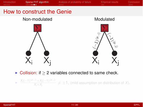
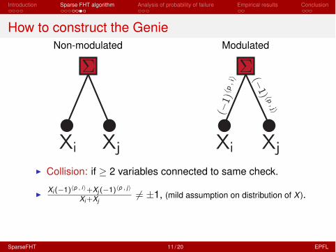
How to construct the GenieNon-modulated Modulated
I Collision: if � 2 variables connected to same check.
I Xi (�1)hp , ii+Xj (�1)hp , ji
Xi+Xj6= ±1, (mild assumption on distribution of X ).
SparseFHT 11 / 20 EPFL
Introduction Sparse FHT algorithm Analysis of probability of failure Empirical results Conclusion
How to construct the GenieNon-modulated Modulated
I Collision: if � 2 variables connected to same check.
I Xi (�1)hp , ii+Xj (�1)hp , ji
Xi+Xj6= ±1, (mild assumption on distribution of X ).
SparseFHT 11 / 20 EPFL

Introduction Sparse FHT algorithm Analysis of probability of failure Empirical results Conclusion
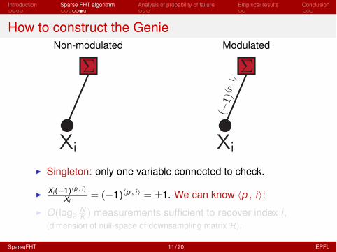
How to construct the GenieNon-modulated Modulated
I Singleton: only one variable connected to check.
I Xi (�1)hp , ii
Xi= (�1)hp , ii = ±1. We can know hp , ii!
I O(log2NK ) measurements sufficient to recover index i ,
(dimension of null-space of downsampling matrix H).
SparseFHT 11 / 20 EPFL

Introduction Sparse FHT algorithm Analysis of probability of failure Empirical results Conclusion
How to construct the GenieNon-modulated Modulated
I Singleton: only one variable connected to check.
I Xi (�1)hp , ii
Xi= (�1)hp , ii = ±1. We can know hp , ii!
I O(log2NK ) measurements sufficient to recover index i ,
(dimension of null-space of downsampling matrix H).
SparseFHT 11 / 20 EPFL
Introduction Sparse FHT algorithm Analysis of probability of failure Empirical results Conclusion
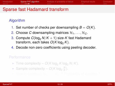
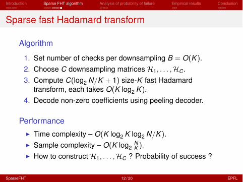
Sparse fast Hadamard transform
Algorithm
1. Set number of checks per downsampling B = O(K ).2. Choose C downsampling matrices H1, . . . ,HC .3. Compute C(log2 N/K + 1) size-K fast Hadamard
transform, each takes O(K log2 K ).4. Decode non-zero coefficients using peeling decoder.
PerformanceI Time complexity – O(K log2 K log2 N/K ).I Sample complexity – O(K log2
NK ).
I How to construct H1, . . . ,HC ? Probability of success ?
SparseFHT 12 / 20 EPFL

Introduction Sparse FHT algorithm Analysis of probability of failure Empirical results Conclusion
Sparse fast Hadamard transform
Algorithm
1. Set number of checks per downsampling B = O(K ).2. Choose C downsampling matrices H1, . . . ,HC .3. Compute C(log2 N/K + 1) size-K fast Hadamard
transform, each takes O(K log2 K ).4. Decode non-zero coefficients using peeling decoder.
PerformanceI Time complexity – O(K log2 K log2 N/K ).I Sample complexity – O(K log2
NK ).
I How to construct H1, . . . ,HC ? Probability of success ?
SparseFHT 12 / 20 EPFL

Introduction Sparse FHT algorithm Analysis of probability of failure Empirical results Conclusion
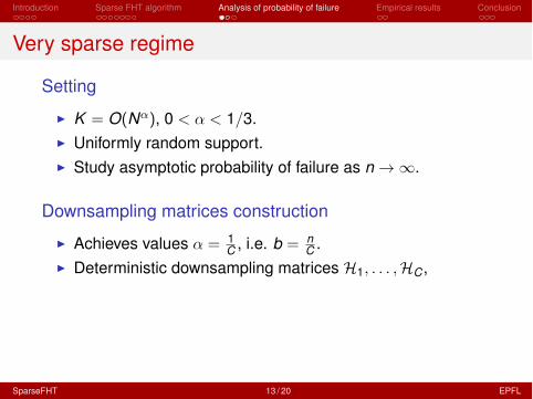
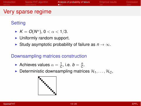
Very sparse regime
Setting
I K = O(N↵), 0 < ↵ < 1/3.I Uniformly random support.I Study asymptotic probability of failure as n!1.
Downsampling matrices construction
I Achieves values ↵ = 1C , i.e. b = n
C .I Deterministic downsampling matrices H1, . . . ,HC ,
SparseFHT 13 / 20 EPFL
Introduction Sparse FHT algorithm Analysis of probability of failure Empirical results Conclusion
Very sparse regime
Setting
I K = O(N↵), 0 < ↵ < 1/3.I Uniformly random support.I Study asymptotic probability of failure as n!1.
Downsampling matrices construction
I Achieves values ↵ = 1C , i.e. b = n
C .I Deterministic downsampling matrices H1, . . . ,HC ,
SparseFHT 13 / 20 EPFL
Introduction Sparse FHT algorithm Analysis of probability of failure Empirical results Conclusion
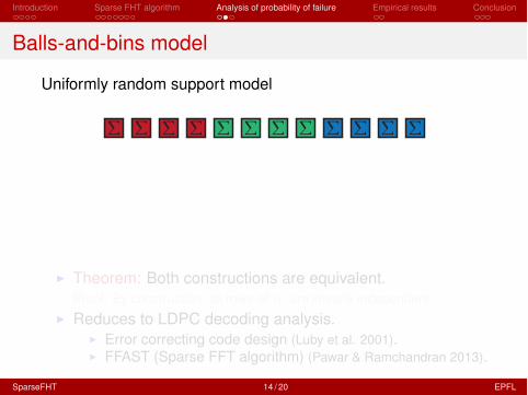
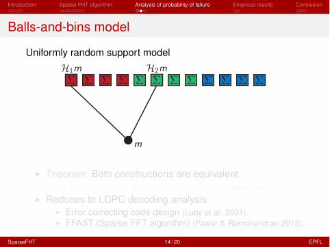
Balls-and-bins model
Uniformly random support model
I Theorem: Both constructions are equivalent.Proof: By construction, all rows of Hi are linearly independent.
I Reduces to LDPC decoding analysis.I Error correcting code design (Luby et al. 2001).I FFAST (Sparse FFT algorithm) (Pawar & Ramchandran 2013).
SparseFHT 14 / 20 EPFL

Introduction Sparse FHT algorithm Analysis of probability of failure Empirical results Conclusion
Balls-and-bins model
Uniformly random support model
I Theorem: Both constructions are equivalent.Proof: By construction, all rows of Hi are linearly independent.
I Reduces to LDPC decoding analysis.I Error correcting code design (Luby et al. 2001).I FFAST (Sparse FFT algorithm) (Pawar & Ramchandran 2013).
SparseFHT 14 / 20 EPFL
Introduction Sparse FHT algorithm Analysis of probability of failure Empirical results Conclusion
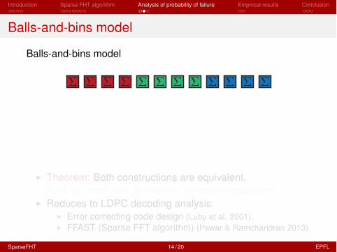
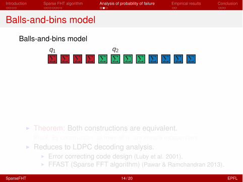
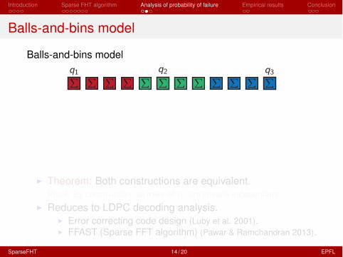
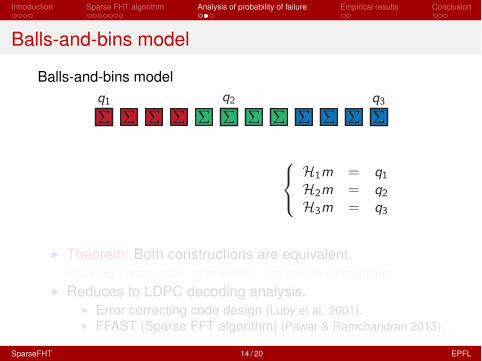
Balls-and-bins model
Balls-and-bins model
I Theorem: Both constructions are equivalent.Proof: By construction, all rows of Hi are linearly independent.
I Reduces to LDPC decoding analysis.I Error correcting code design (Luby et al. 2001).I FFAST (Sparse FFT algorithm) (Pawar & Ramchandran 2013).
SparseFHT 14 / 20 EPFL

Introduction Sparse FHT algorithm Analysis of probability of failure Empirical results Conclusion
Balls-and-bins model
Balls-and-bins model
I Theorem: Both constructions are equivalent.Proof: By construction, all rows of Hi are linearly independent.
I Reduces to LDPC decoding analysis.I Error correcting code design (Luby et al. 2001).I FFAST (Sparse FFT algorithm) (Pawar & Ramchandran 2013).
SparseFHT 14 / 20 EPFL

Introduction Sparse FHT algorithm Analysis of probability of failure Empirical results Conclusion
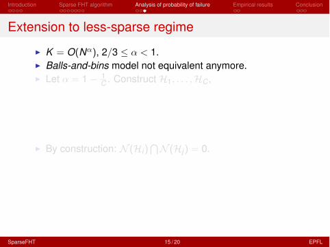
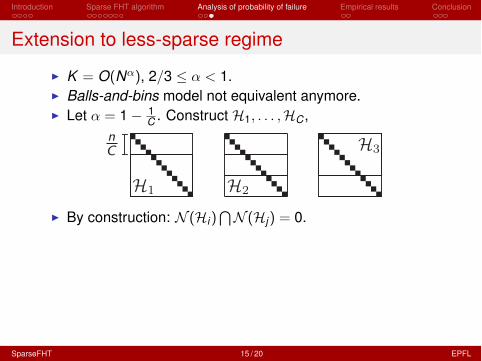
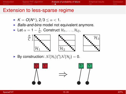
Extension to less-sparse regime
I K = O(N↵), 2/3 ↵ < 1.I Balls-and-bins model not equivalent anymore.I Let ↵ = 1� 1
C . Construct H1, . . . ,HC ,
I By construction: N (Hi)TN (Hj) = 0.
SparseFHT 15 / 20 EPFL
Introduction Sparse FHT algorithm Analysis of probability of failure Empirical results Conclusion
Extension to less-sparse regime
I K = O(N↵), 2/3 ↵ < 1.I Balls-and-bins model not equivalent anymore.I Let ↵ = 1� 1
C . Construct H1, . . . ,HC ,
I By construction: N (Hi)TN (Hj) = 0.
SparseFHT 15 / 20 EPFL

Introduction Sparse FHT algorithm Analysis of probability of failure Empirical results Conclusion
SparseFHT – Probability of successProbability of success - N = 222
0 1/3 2/3 10
0.2
0.4
0.6
0.8
1
↵SparseFHT 16 / 20 EPFL
Introduction Sparse FHT algorithm Analysis of probability of failure Empirical results Conclusion
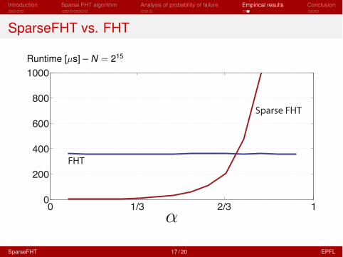
SparseFHT vs. FHT
Runtime [µs] – N = 215
0 1/3 2/3 10
200
400
600
800
1000
Sparse FHT
FHT
↵
SparseFHT 17 / 20 EPFL
Introduction Sparse FHT algorithm Analysis of probability of failure Empirical results Conclusion
Conclusion
ContributionI Sparse fast Hadamard algorithm.I Time complexity O(K log2 K log2
NK ).
I Sample complexity O(K log2NK ).
I Probability of success asymptotically equal to 1.
What’s next ?I Investigate noisy case.
SparseFHT 18 / 20 EPFL

Introduction Sparse FHT algorithm Analysis of probability of failure Empirical results Conclusion
Thanks for your attention!
Code and figures available athttp://lcav.epfl.ch/page-99903.html
SparseFHT 19 / 20 EPFL

Introduction Sparse FHT algorithm Analysis of probability of failure Empirical results Conclusion
Reference
[1] M.G. Luby, M. Mitzenmacher, M.A. Shokrollahi, andD.A. Spielman,Efficient erasure correcting codes,IEEE Trans. Inform. Theory, vol. 47, no. 2,pp. 569–584, 2001.
[2] S. Pawar and K. Ramchandran,Computing a k-sparse n-length discrete Fourier transformusing at most 4k samples and O(k log k) complexity,arXiv.org, vol. cs.DS. 04-May-2013.
SparseFHT 20 / 20 EPFL


![Model-based Compressive Sensing - …people.ee.duke.edu/~lcarin/baraniuk.pdf[Eldar, Mishali], [Baron, Duarte et al], [B, C, Duarte, Hegde] • Ex: clustered signals ... sparsity](https://img.pdfslide.net/doc/110x75/5b0607667f8b9ad1768c3ce6/model-based-compressive-sensing-lcarinbaraniukpdfeldar-mishali-baron-duarte.jpg)


![Fast Background Initialization with Recursive Hadamard ... · 2. The Hadamard Transform The Hadamard transform [7, 9] belongs to the gener-alized class of Fourier transforms and it](https://img.pdfslide.net/doc/110x75/5f13c09011c737592655ec87/fast-background-initialization-with-recursive-hadamard-2-the-hadamard-transform.jpg)