1

Chapter 25ODE : Initial-value problem 1

2

When dealing with an nth-order differentialequation, n conditions are required to obtain aunique solution.

If all conditions are specified at the same value ofthe independent variable (for example, atx or t = 0),then the problemis called aninitial-value problem.

This is in contrast toboundary-value problemswhere specification of conditions occurs at differentvalues of the independent variable.

3

The Unified Form of Solving ODE

( )dxyx,fdy =

( )hh,y,xyy iii1i φ+=+

Depending on function φφφφ, there are different solutions.

The Runge-Kutta methods are the most popular.

00ii xx at y condition initial and xxh =−= +1

( )yx,fdx

dy =

4

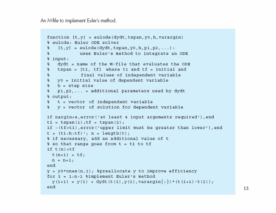
The Euler’s Method

( )iixx

y,xfdx

dy

i

===

φ

Error estimate:( )

nn

ni2i

iii Rhn!

yh

2!

yhyyy +++

′′+′+=+ L1

( ) ( ) ( ) ( )( )n

nii1-n

3ii2iiiiii Rh

n!

y,xfh

3!

y,xfh

2!

y,xfhy,xfyy ++

′′+

′++=+ L1

Et = Et,2 + Et,3 + … + Et,n

Differential equation evaluated at xi and yi

5

Example 1 of Euler’s Method

6

7

Example 2

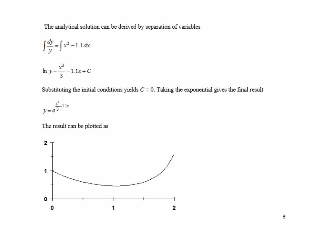
8

9

X0 =y0 =

X1 =

Example 3

10

11

12

13

14

General Idea of Runge-Kutta Methods

Given the order n, the coefficients ai, pi, and qij are determined by equaling terms to the Taylor series.

( )hh,y,xyy iiii φ+=+1

15

16

Various 2 nd-order Runge-Kutta Methods

17

18

Example 4

19

20

21

22

Comparison of Various 2 nd-order RK Methods

Integrate f(x,y) = -2x3 + 12x2 – 20x + 8.5

from x = 0 to x = 4 using a step size of 0.5, with initial condition y = 1 at x = 0.

23

24

Classical 4 th-order RK Method

25

26

27

Example

28

29

30

31

Classical 5 th-order RK Method

32

Comparison of RK Methods of Different Orders

Integrate f(x,y) = 4e0.8x – 0.5ywith y(0) = 2 from x = a = 0 to x = b = 4 using various step sizes. Compare the accuracy of the

various methods for the result at x = 4 based on the exact answer of y(4) = 75.33896

h

abnEffort f

−=

nf is the number of function evaluations involved in the particular RK computation.

Example: when n = 4, we need to calculate k1 through k4, hence 4 evaluations of f(x,y); so nf = 4.

Inspection of the figure leads to a number of conclusions: first, that the higher-order methods attain better accuracy for the same computational effort and, second, that the gain in accuracy for the additional effort tends to diminish after a point. (Notice that the curves drop rapidly at first and then tend to level off.)

Systems of ODEs

34

Euler’s Method for System of ODEs

35

4th-order RK Method for System of ODEs

122

11

104 y0.3ydx

dy

0.5ydx

dy

.−−=

−=

Initial conditions: y1(0) = 4, y2(0) = 6

Integrate from x = 0 to x= 2 with 0.5 step size

36

Example

Cd = 0.25

37

38

Example of System of ODEs

( )

−=

=

34

4

y16.1sindt

dy

ydt

dy3

−=

=

12

2

16.1ydt

dy

ydt

dy1

y1 = θ, y2 = dθ/dt

0116 =+ sinθdt

θd2

2

.

(linear approximation when θ is small)

y3 = θ, y4 = dθ/dt

(exact conversion)

small initial θ large initial θ

39

Special Problem 8

40

Special Problem 9

Homework

41

1.

2.

3.

4.

5.

Homework

42

6.