Embed Size (px)
Citation preview

Chapter-1 and 2
Subject: FIP (181102)Prof. Asodariya Bhavesh
ECD,SSASIT, Surat
Digital Image Processing, 3rd edition by Gonzalez and Woods
Optics and Human Vision
The physics of light
http://commons.wikimedia.org/wiki/File:Eye-diagram_bg.svg
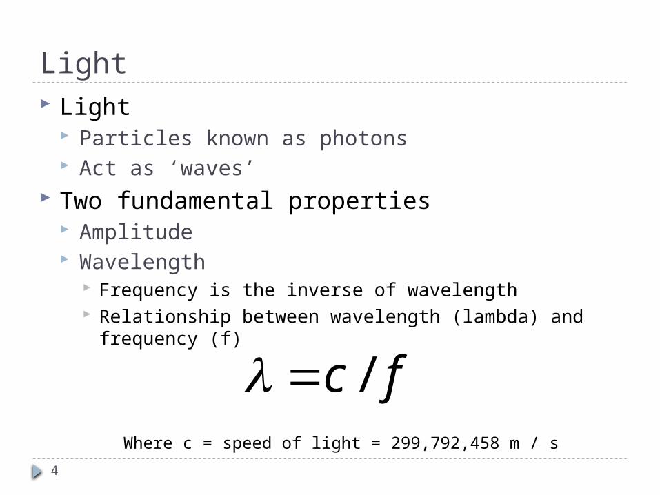
Light Light
Particles known as photons Act as ‘waves’
Two fundamental properties Amplitude Wavelength
Frequency is the inverse of wavelength Relationship between wavelength (lambda) and
frequency (f)
fc /Where c = speed of light = 299,792,458 m / s
4
What is Digital Image Processing?Digital image processing focuses on two major tasks
Improvement of pictorial information for human interpretation
Processing of image data for storage, transmission and representation for autonomous machine perception
Some argument about where image processing ends and fields such as image analysis and computer vision start
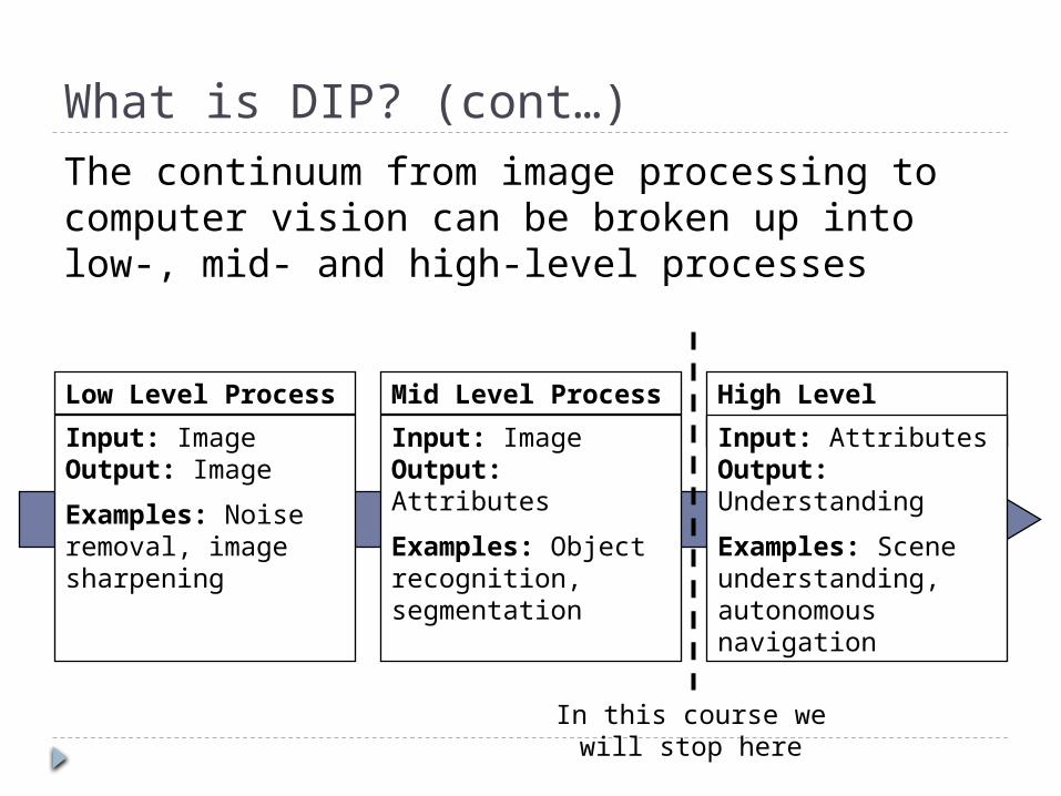
What is DIP? (cont…)The continuum from image processing to computer vision can be broken up into low-, mid- and high-level processes
Low Level ProcessInput: ImageOutput: ImageExamples: Noise removal, image sharpening
Mid Level ProcessInput: Image Output: AttributesExamples: Object recognition, segmentation
High Level ProcessInput: Attributes Output: UnderstandingExamples: Scene understanding, autonomous navigation
In this course we will stop here
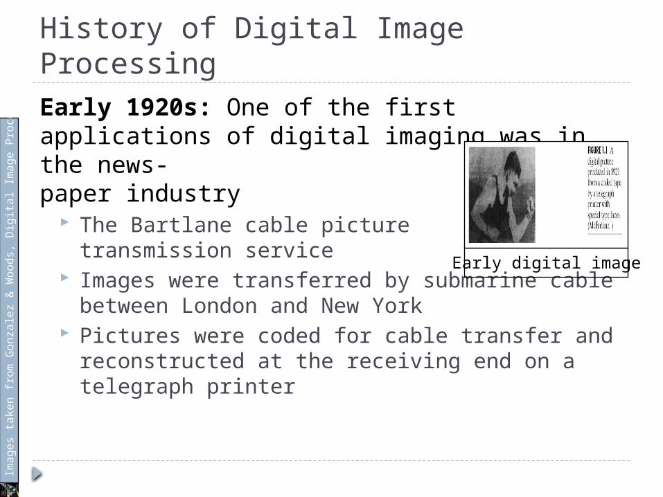
History of Digital Image ProcessingEarly 1920s: One of the first applications of digital imaging was in the news-paper industry
The Bartlane cable picture transmission service
Images were transferred by submarine cable between London and New York
Pictures were coded for cable transfer and reconstructed at the receiving end on a telegraph printer
Early digital image
Imag
es ta
ken
from
Gon
zale
z & W
oods
, Dig
ital I
mag
e Pr
oces
sing
(200
2)
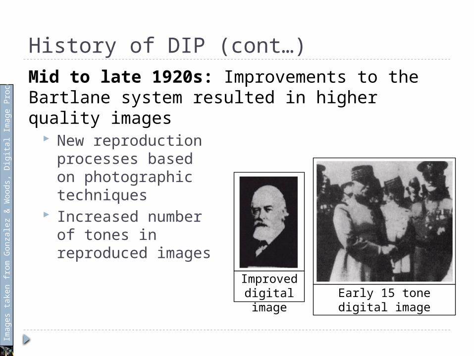
History of DIP (cont…)Mid to late 1920s: Improvements to the Bartlane system resulted in higher quality images
New reproduction processes based on photographic techniques
Increased number of tones in reproduced images
Improved digital image
Early 15 tone digital image
Imag
es ta
ken
from
Gon
zale
z & W
oods
, Dig
ital I
mag
e Pr
oces
sing
(200
2)
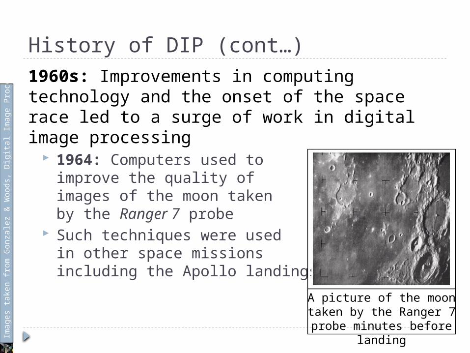
History of DIP (cont…)1960s: Improvements in computing technology and the onset of the space race led to a surge of work in digital image processing
1964: Computers used to improve the quality of images of the moon taken by the Ranger 7 probe
Such techniques were usedin other space missions including the Apollo landings
A picture of the moon taken by the Ranger 7 probe minutes before
landing
Imag
es ta
ken
from
Gon
zale
z & W
oods
, Dig
ital I
mag
e Pr
oces
sing
(200
2)
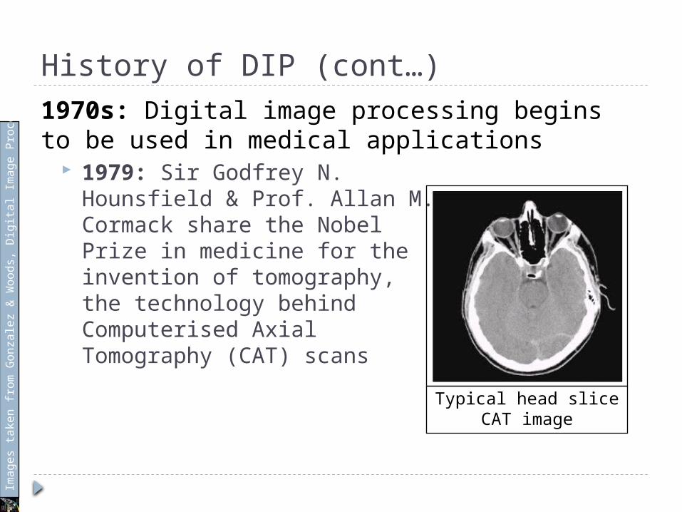
History of DIP (cont…)1970s: Digital image processing begins to be used in medical applications
1979: Sir Godfrey N. Hounsfield & Prof. Allan M. Cormack share the Nobel Prize in medicine for the invention of tomography, the technology behind Computerised Axial Tomography (CAT) scans
Typical head slice CAT image
Imag
es ta
ken
from
Gon
zale
z & W
oods
, Dig
ital I
mag
e Pr
oces
sing
(200
2)
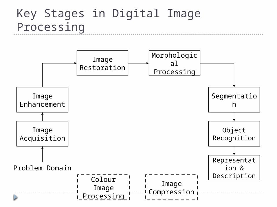
Key Stages in Digital Image Processing
Image Acquisition
Image Restoration
Morphological Processing
Segmentation
Representation &
Description
Image Enhancemen
t
Object Recognition
Problem DomainColour Image
ProcessingImage
Compression
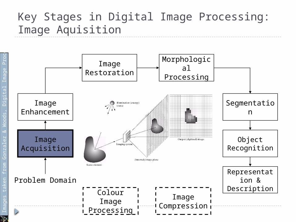
Key Stages in Digital Image Processing:Image Aquisition
Image Acquisition
Image Restoration
Morphological Processing
Segmentation
Representation &
Description
Image Enhancemen
t
Object Recognition
Problem DomainColour Image
ProcessingImage
Compression
Imag
es ta
ken
from
Gon
zale
z & W
oods
, Dig
ital I
mag
e Pr
oces
sing
(200
2)
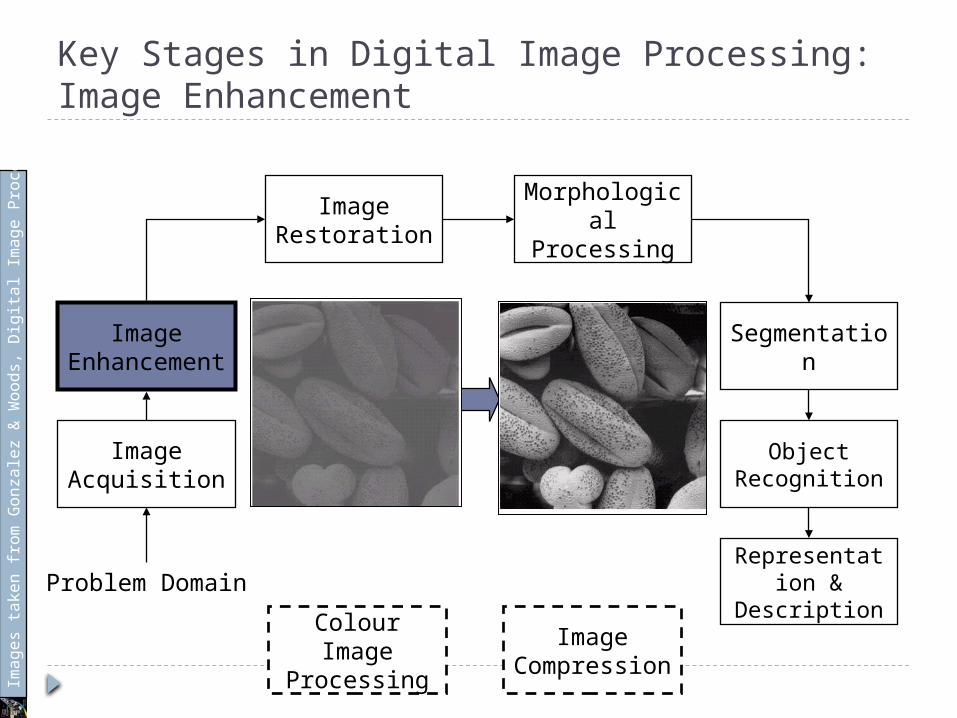
Key Stages in Digital Image Processing:Image Enhancement
Image Acquisition
Image Restoration
Morphological Processing
Segmentation
Representation &
Description
Image Enhancemen
t
Object Recognition
Problem DomainColour Image
ProcessingImage
Compression
Imag
es ta
ken
from
Gon
zale
z & W
oods
, Dig
ital I
mag
e Pr
oces
sing
(200
2)
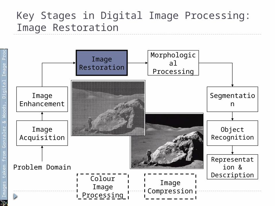
Key Stages in Digital Image Processing:Image Restoration
Image Acquisition
Image Restoration
Morphological Processing
Segmentation
Representation &
Description
Image Enhancemen
t
Object Recognition
Problem DomainColour Image
ProcessingImage
Compression
Imag
es ta
ken
from
Gon
zale
z & W
oods
, Dig
ital I
mag
e Pr
oces
sing
(200
2)
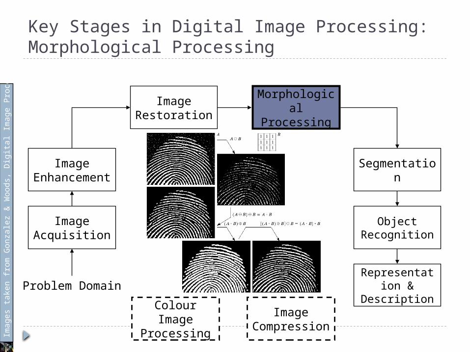
Key Stages in Digital Image Processing:Morphological Processing
Image Acquisition
Image Restoration
Morphological Processing
Segmentation
Representation &
Description
Image Enhancemen
t
Object Recognition
Problem DomainColour Image
ProcessingImage
Compression
Imag
es ta
ken
from
Gon
zale
z & W
oods
, Dig
ital I
mag
e Pr
oces
sing
(200
2)
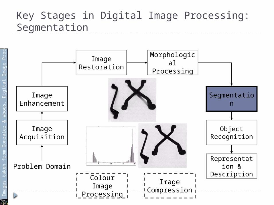
Key Stages in Digital Image Processing:Segmentation
Image Acquisition
Image Restoration
Morphological Processing
Segmentation
Representation &
Description
Image Enhancemen
t
Object Recognition
Problem DomainColour Image
ProcessingImage
Compression
Imag
es ta
ken
from
Gon
zale
z & W
oods
, Dig
ital I
mag
e Pr
oces
sing
(200
2)
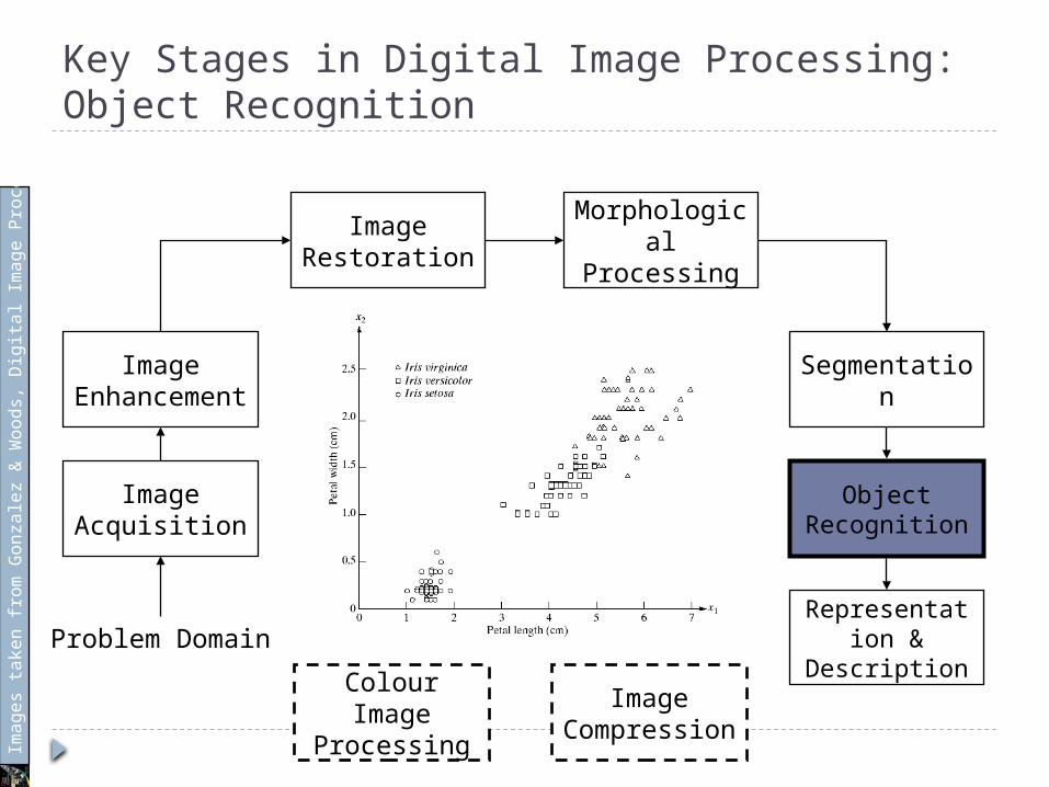
Key Stages in Digital Image Processing:Object Recognition
Image Acquisition
Image Restoration
Morphological Processing
Segmentation
Representation &
Description
Image Enhancemen
t
Object Recognition
Problem DomainColour Image
ProcessingImage
Compression
Imag
es ta
ken
from
Gon
zale
z & W
oods
, Dig
ital I
mag
e Pr
oces
sing
(200
2)
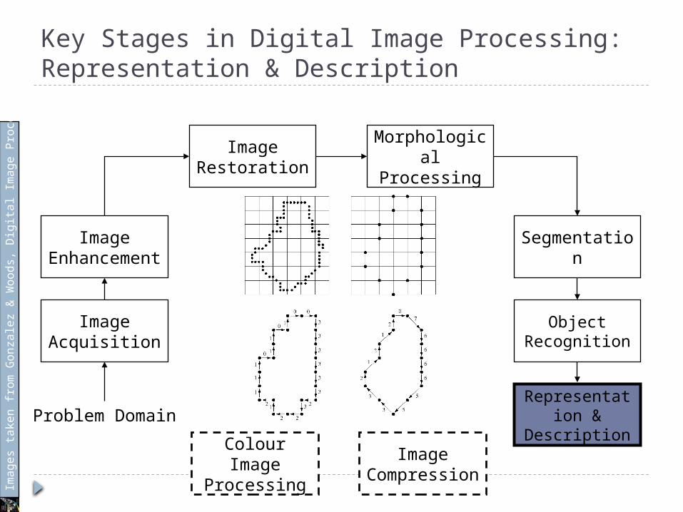
Key Stages in Digital Image Processing:Representation & Description
Image Acquisition
Image Restoration
Morphological Processing
Segmentation
Representation &
Description
Image Enhancemen
t
Object Recognition
Problem DomainColour Image
ProcessingImage
Compression
Imag
es ta
ken
from
Gon
zale
z & W
oods
, Dig
ital I
mag
e Pr
oces
sing
(200
2)
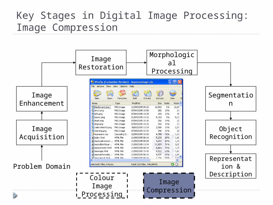
Key Stages in Digital Image Processing:Image Compression
Image Acquisition
Image Restoration
Morphological Processing
Segmentation
Representation &
Description
Image Enhancemen
t
Object Recognition
Problem DomainColour Image
ProcessingImage
Compression
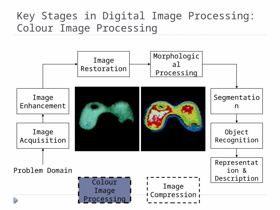
Key Stages in Digital Image Processing:Colour Image Processing
Image Acquisition
Image Restoration
Morphological Processing
Segmentation
Representation &
Description
Image Enhancemen
t
Object Recognition
Problem DomainColour Image
ProcessingImage
Compression
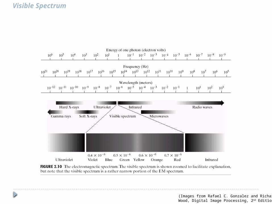
Visible Spectrum
(Images from Rafael C. Gonzalez and Richard E. Wood, Digital Image Processing, 2nd Edition.
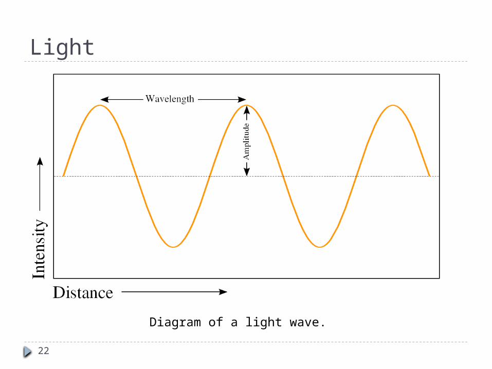
Light
Diagram of a light wave.
22
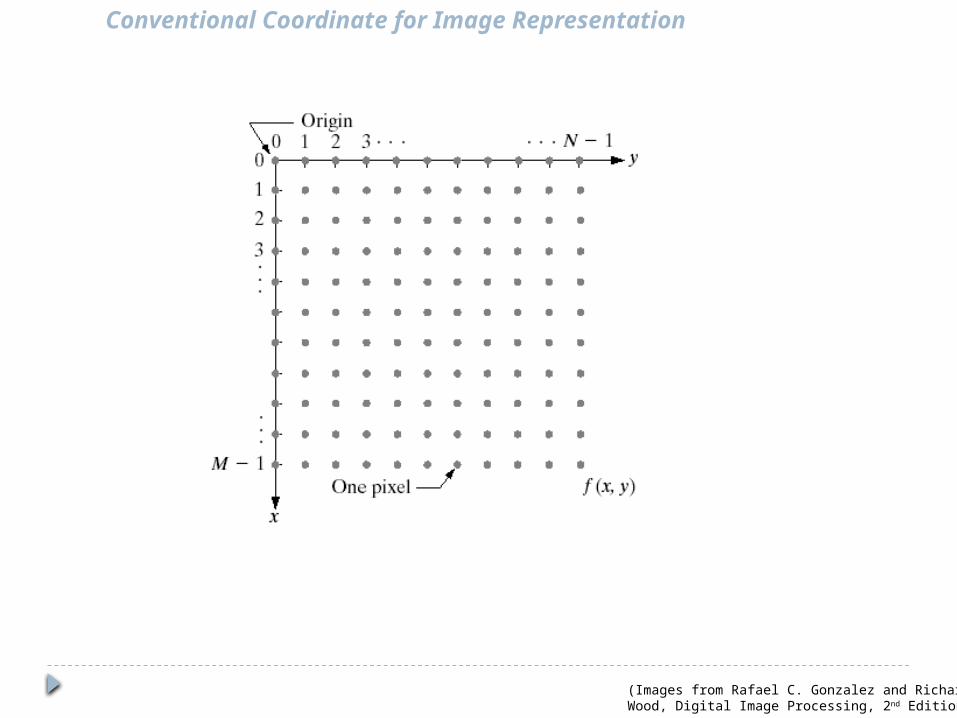
Conventional Coordinate for Image Representation
(Images from Rafael C. Gonzalez and Richard E. Wood, Digital Image Processing, 2nd Edition.
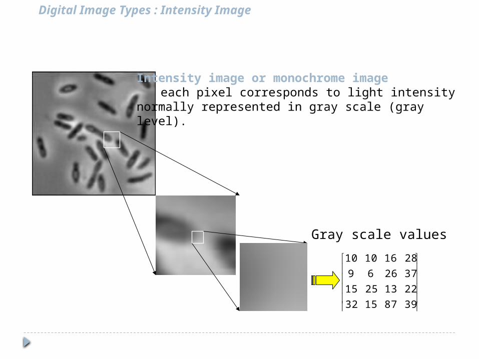
Digital Image Types : Intensity Image
Intensity image or monochrome image each pixel corresponds to light intensitynormally represented in gray scale (gray level).
398715322213251537266928161010
Gray scale values
398715322213251537266928161010
39656554424754216796543243567065
99876532924385856796906078567099
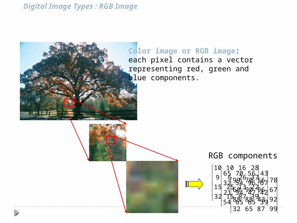
Digital Image Types : RGB Image
Color image or RGB image:each pixel contains a vectorrepresenting red, green andblue components.
RGB components
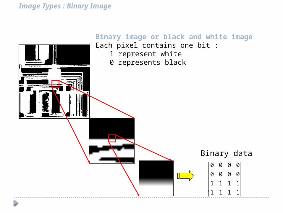
Image Types : Binary Image
Binary image or black and white imageEach pixel contains one bit :
1 represent white0 represents black
1111111100000000
Binary data
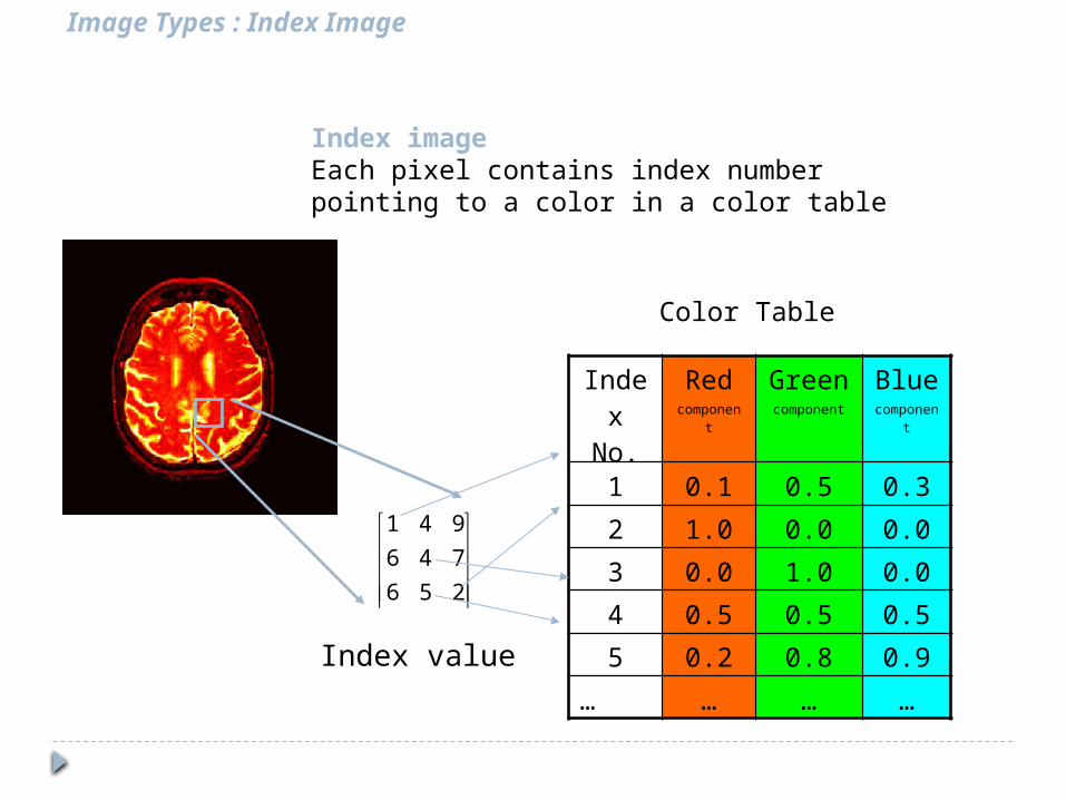
Image Types : Index Image
Index imageEach pixel contains index numberpointing to a color in a color table
256746941
Index value
Index No.
Redcomponent
Greencomponent
Bluecomponent
1 0.1 0.5 0.32 1.0 0.0 0.03 0.0 1.0 0.04 0.5 0.5 0.55 0.2 0.8 0.9
… … … …
Color Table
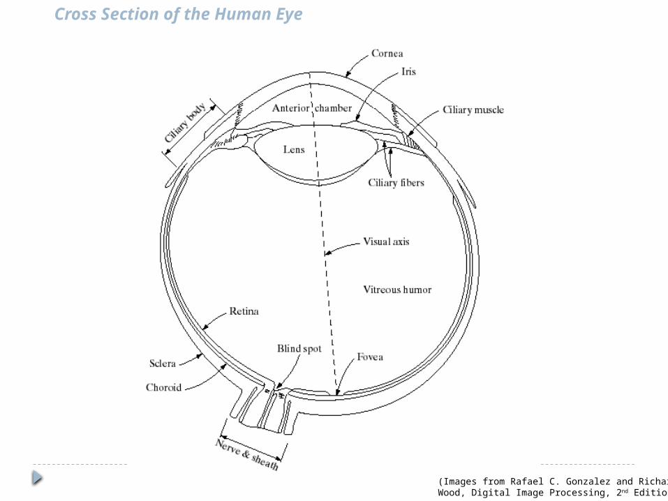
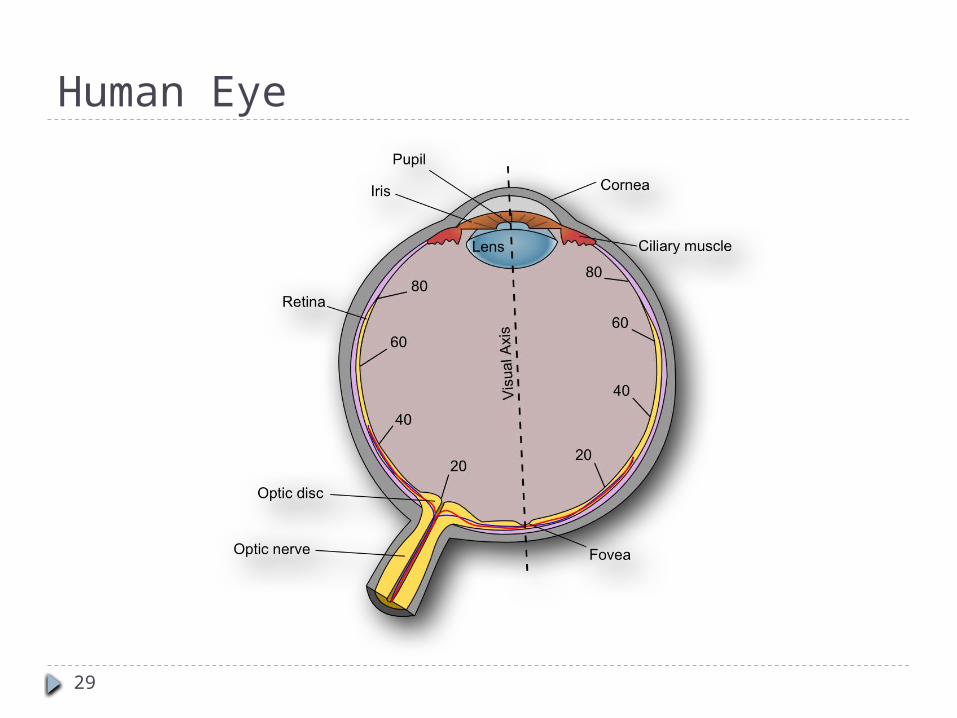
Cross Section of the Human Eye
(Images from Rafael C. Gonzalez and Richard E. Wood, Digital Image Processing, 2nd Edition.
29
Human Eye
30
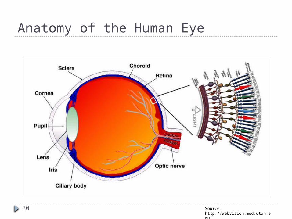
Anatomy of the Human Eye
Source: http://webvision.med.utah.edu/
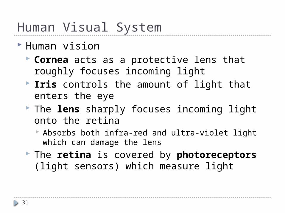
Human Visual System Human vision
Cornea acts as a protective lens that roughly focuses incoming light
Iris controls the amount of light that enters the eye
The lens sharply focuses incoming light onto the retina Absorbs both infra-red and ultra-violet light which can
damage the lens The retina is covered by photoreceptors (light
sensors) which measure light
31

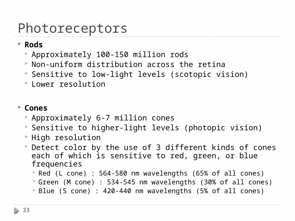
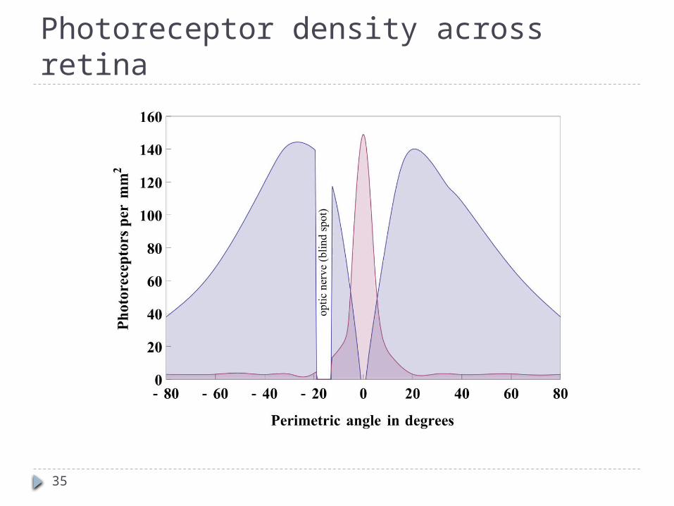
Photoreceptors Rods
Approximately 100-150 million rods Non-uniform distribution across the retina Sensitive to low-light levels (scotopic vision) Lower resolution
Cones Approximately 6-7 million cones Sensitive to higher-light levels (photopic vision) High resolution Detect color by the use of 3 different kinds of cones each
of which is sensitive to red, green, or blue frequencies Red (L cone) : 564-580 nm wavelengths (65% of all cones) Green (M cone) : 534-545 nm wavelengths (30% of all cones) Blue (S cone) : 420-440 nm wavelengths (5% of all cones)
33
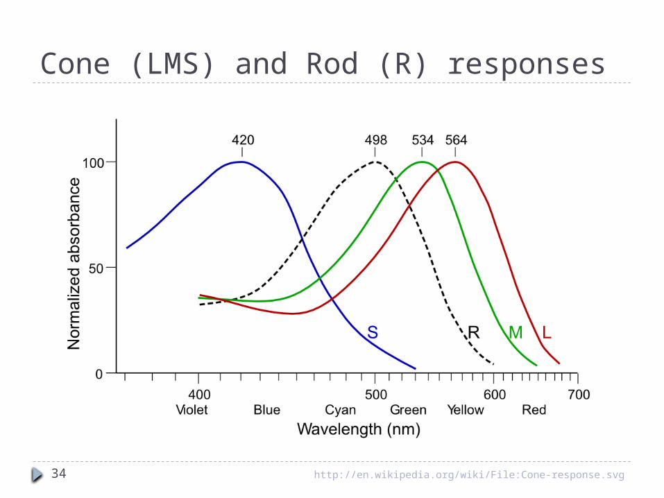
Cone (LMS) and Rod (R) responses
http://en.wikipedia.org/wiki/File:Cone-response.svg34
35
Photoreceptor density across retina
36
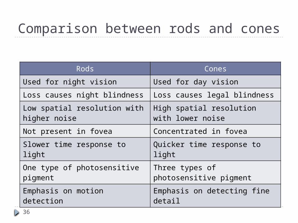
Comparison between rods and cones
Rods ConesUsed for night vision Used for day visionLoss causes night blindness Loss causes legal blindnessLow spatial resolution with higher noise
High spatial resolution with lower noise
Not present in fovea Concentrated in foveaSlower time response to light Quicker time response to lightOne type of photosensitive pigment
Three types of photosensitive pigment
Emphasis on motion detection Emphasis on detecting fine detail
Color and Human Perception Chromatic light
has a color component
Achromatic light has no color component has only one property – intensity
37
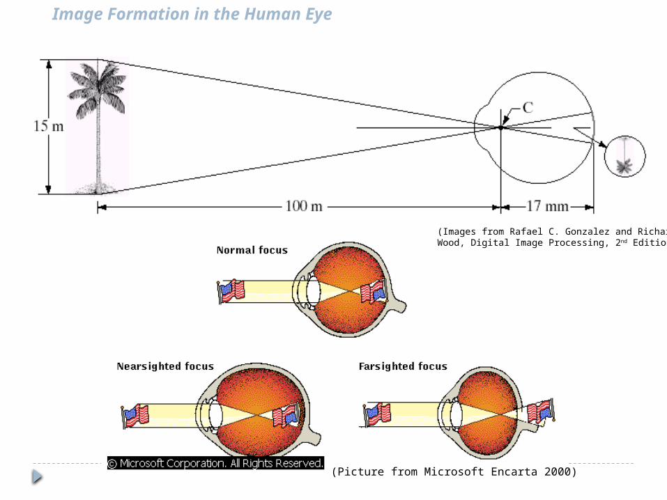
Image Formation in the Human Eye
(Picture from Microsoft Encarta 2000)
(Images from Rafael C. Gonzalez and Richard E. Wood, Digital Image Processing, 2nd Edition.
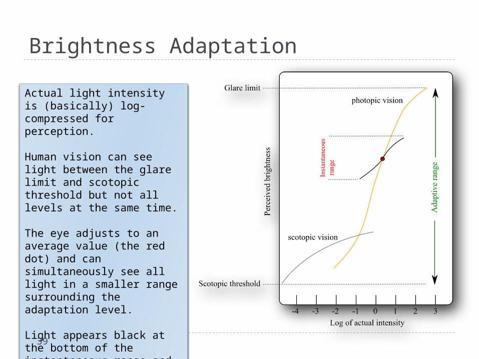
Brightness AdaptationActual light intensity is (basically) log-compressed for perception.
Human vision can see light between the glare limit and scotopic threshold but not all levels at the same time.
The eye adjusts to an average value (the red dot) and can simultaneously see all light in a smaller range surrounding the adaptation level.
Light appears black at the bottom of the instantaneous range and white at the top of that range.39
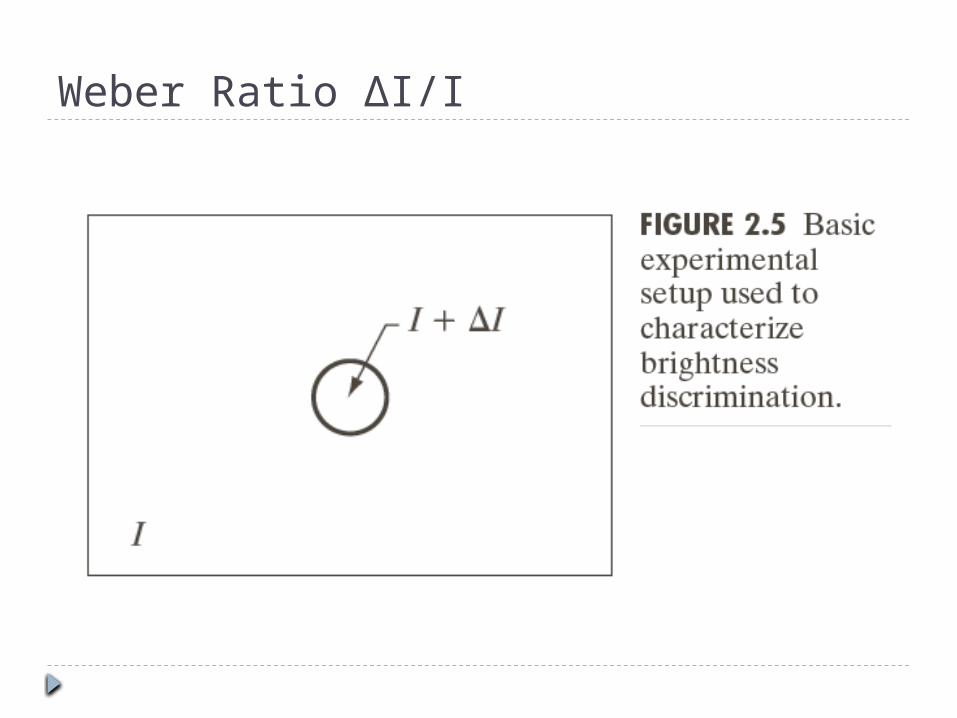
Weber Ratio ∆I/I
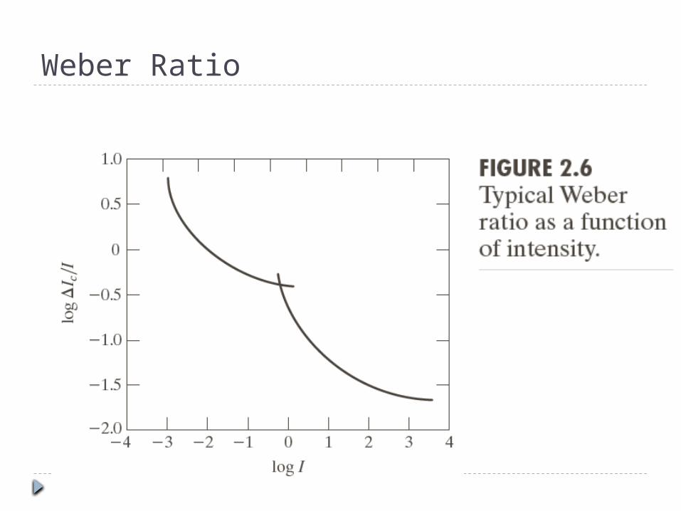
Weber Ratio
42
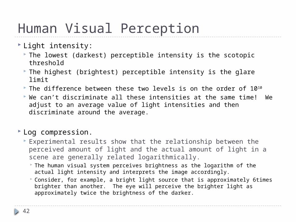
Human Visual Perception Light intensity:
The lowest (darkest) perceptible intensity is the scotopic threshold The highest (brightest) perceptible intensity is the glare limit The difference between these two levels is on the order of 1010
We can’t discriminate all these intensities at the same time! We adjust to an average value of light intensities and then discriminate around the average.
Log compression. Experimental results show that the relationship between the
perceived amount of light and the actual amount of light in a scene are generally related logarithmically. The human visual system perceives brightness as the logarithm of the actual
light intensity and interprets the image accordingly. Consider, for example, a bright light source that is approximately 6times
brighter than another. The eye will perceive the brighter light as approximately twice the brightness of the darker.
43
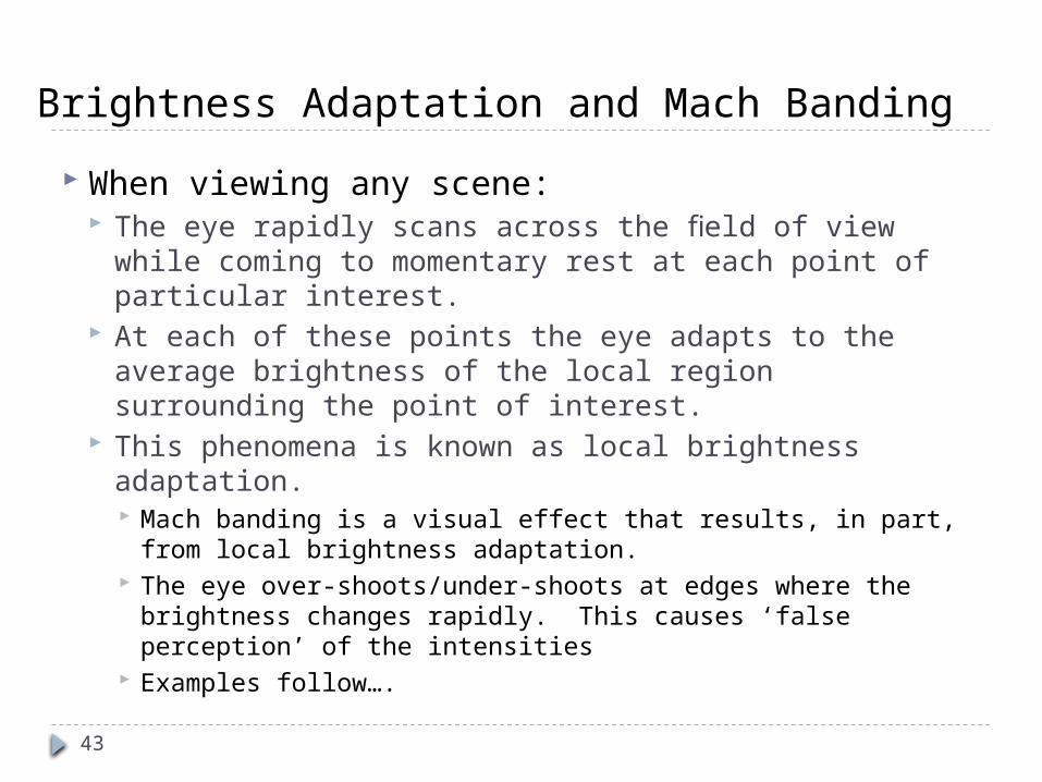
Brightness Adaptation and Mach Banding When viewing any scene:
The eye rapidly scans across the field of view while coming to momentary rest at each point of particular interest.
At each of these points the eye adapts to the average brightness of the local region surrounding the point of interest.
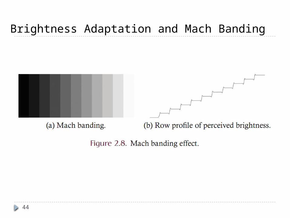
This phenomena is known as local brightness adaptation. Mach banding is a visual effect that results, in part, from local
brightness adaptation. The eye over-shoots/under-shoots at edges where the
brightness changes rapidly. This causes ‘false perception’ of the intensities
Examples follow….
44
Brightness Adaptation and Mach Banding
45
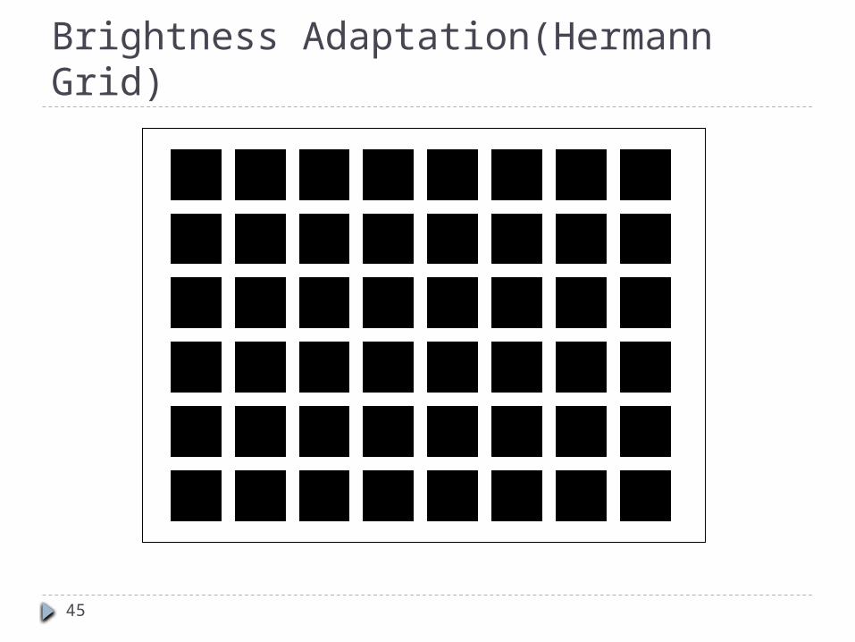
Brightness Adaptation(Hermann Grid)
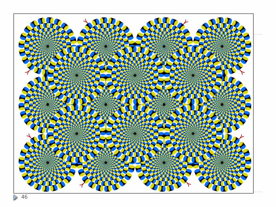
46
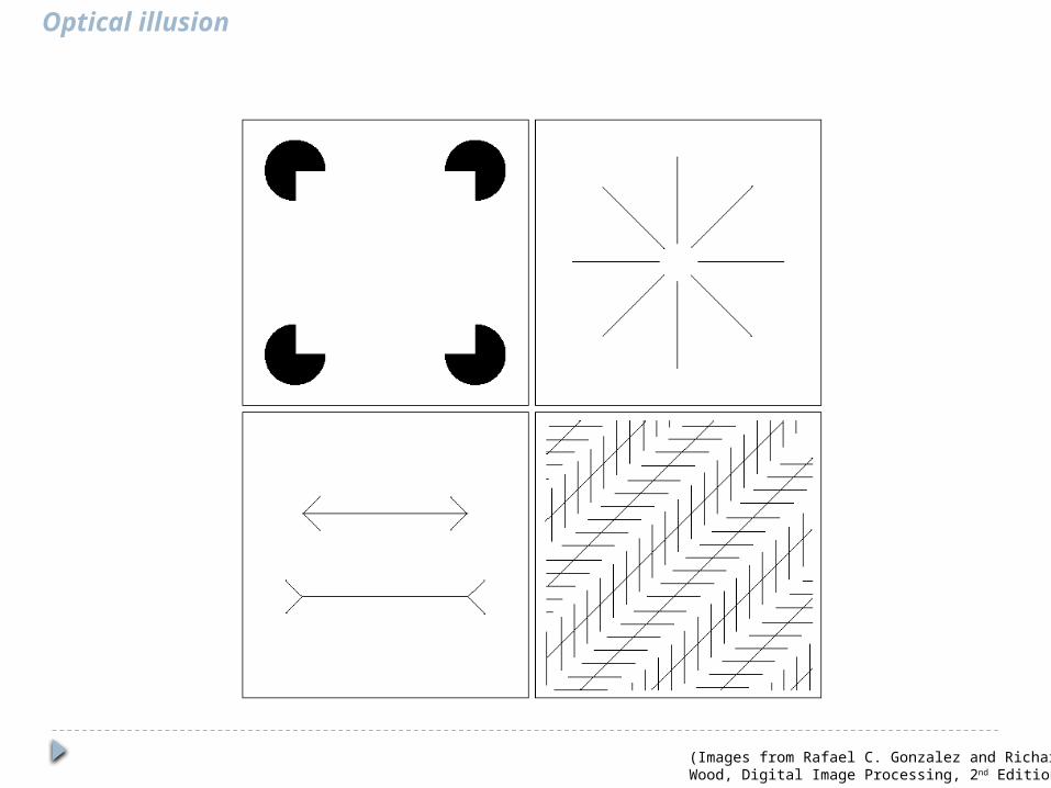
Optical illusion
(Images from Rafael C. Gonzalez and Richard E. Wood, Digital Image Processing, 2nd Edition.
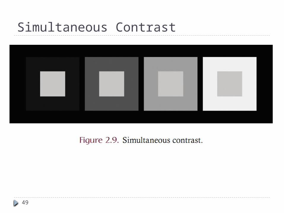
Simultaneous Contrast Simultaneous contrast refers to the way in which
two adjacent intensities (or colors) affect each other. Example: Note that a blank sheet of paper may
appear white when placed on a desktop but may appear black when used to shield the eyes against the sun.
Figure 2.9 is a common way of illustrating that the perceived intensity of a region is dependent upon the contrast of the region with its local background. The four inner squares are of identical intensity but are
contextualized by the four surrounding squares The perceived intensity of the inner squares varies from
bright on the left to dark on the right.
48
49
Simultaneous Contrast
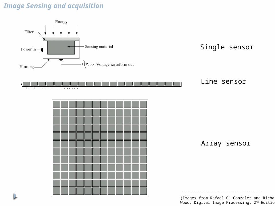
Image Sensing and acquisition
Single sensor
Line sensor
Array sensor
(Images from Rafael C. Gonzalez and Richard E. Wood, Digital Image Processing, 2nd Edition.
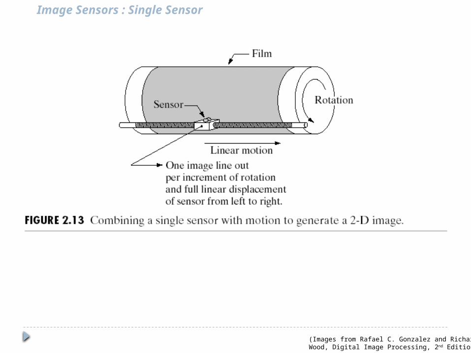
Image Sensors : Single Sensor
(Images from Rafael C. Gonzalez and Richard E. Wood, Digital Image Processing, 2nd Edition.
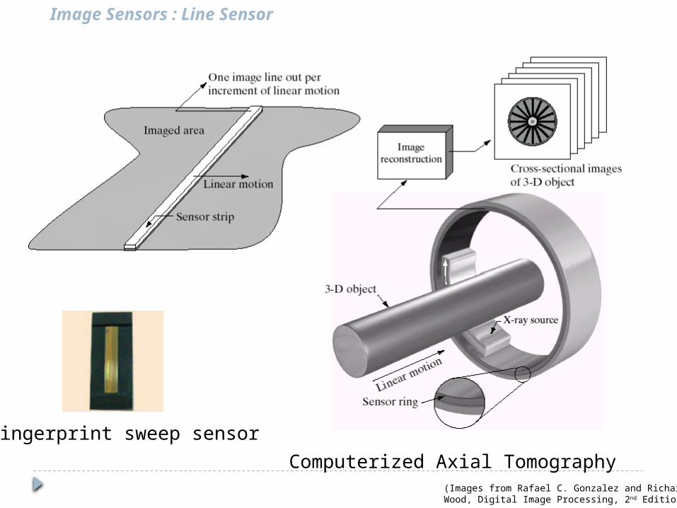
Image Sensors : Line Sensor
Fingerprint sweep sensorComputerized Axial Tomography
(Images from Rafael C. Gonzalez and Richard E. Wood, Digital Image Processing, 2nd Edition.
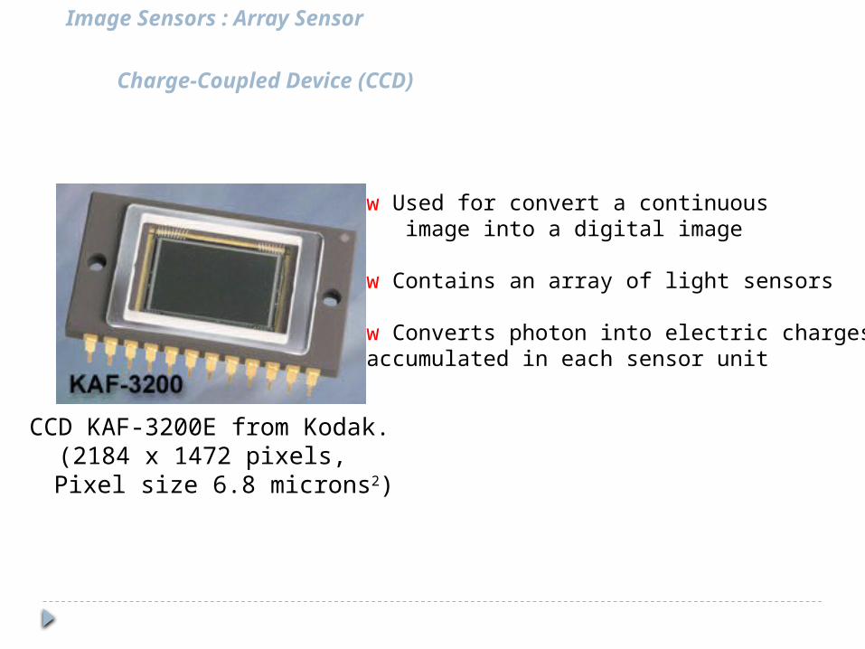
CCD KAF-3200E from Kodak.(2184 x 1472 pixels,
Pixel size 6.8 microns2)
Charge-Coupled Device (CCD)
w Used for convert a continuous image into a digital image
w Contains an array of light sensors
w Converts photon into electric chargesaccumulated in each sensor unit
Image Sensors : Array Sensor
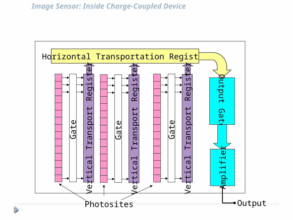
Horizontal Transportation RegisterOutput Gate
Ampl
ifier
Verti
cal T
rans
port
Regi
ster
Gate
Verti
cal T
rans
port
Regi
ster
Gate
Verti
cal T
rans
port
Regi
ster
Gate
Photosites Output
Image Sensor: Inside Charge-Coupled Device
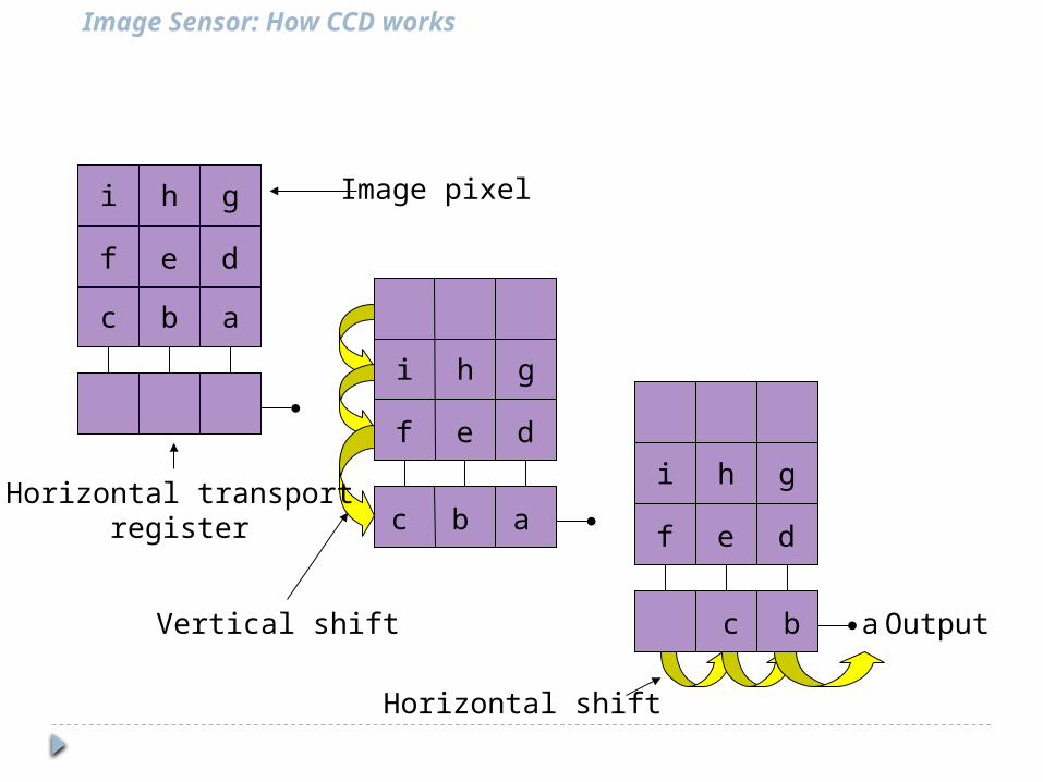
Image Sensor: How CCD works
abc
ghi
def
abc
ghi
def
abc
ghi
def
Vertical shift
Horizontal shift
Image pixel
Horizontal transportregister
Output

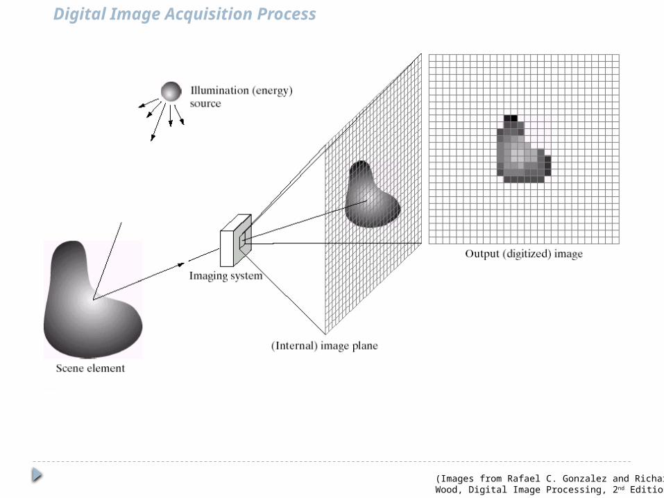
Digital Image Acquisition Process
(Images from Rafael C. Gonzalez and Richard E. Wood, Digital Image Processing, 2nd Edition.
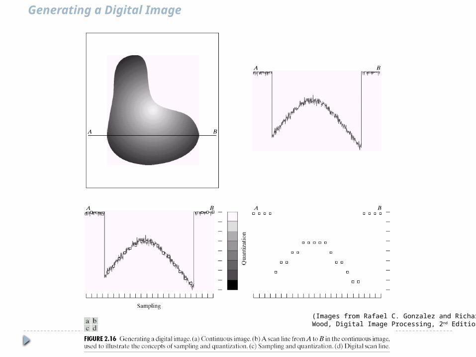
Generating a Digital Image
(Images from Rafael C. Gonzalez and Richard E. Wood, Digital Image Processing, 2nd Edition.
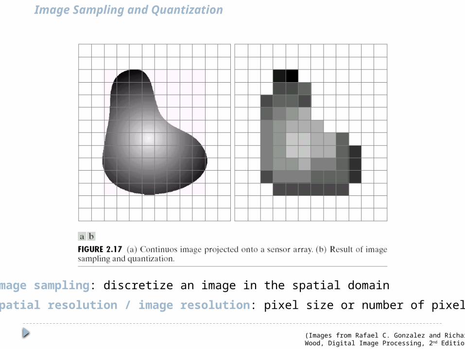
Image Sampling and Quantization
Image sampling: discretize an image in the spatial domainSpatial resolution / image resolution: pixel size or number of pixels
(Images from Rafael C. Gonzalez and Richard E. Wood, Digital Image Processing, 2nd Edition.
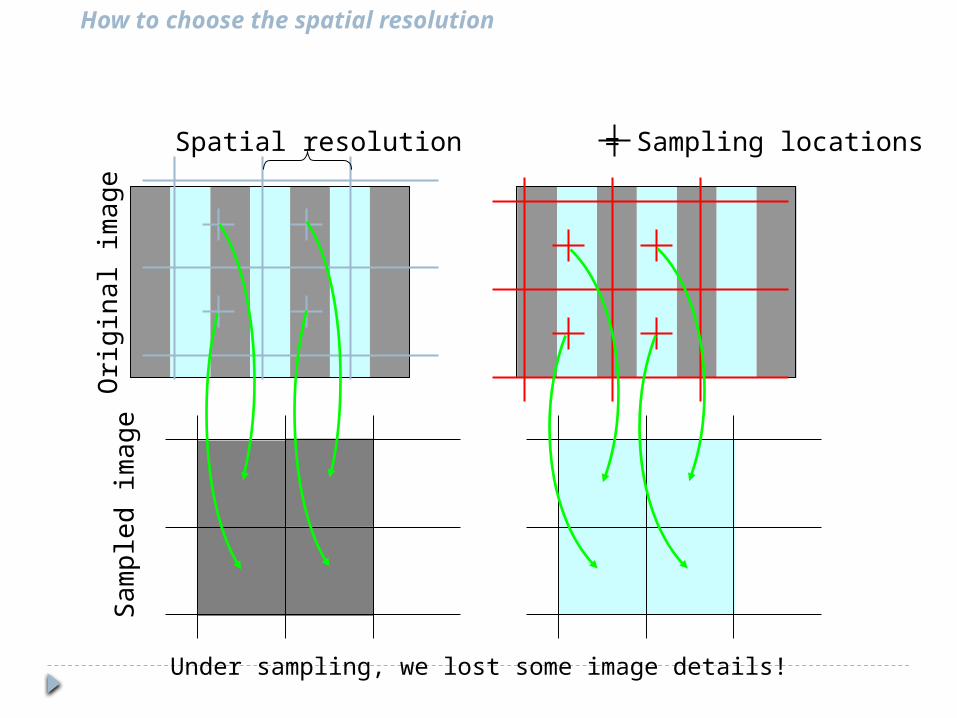
How to choose the spatial resolution
= Sampling locationsOr
igin
al im
age
Sam
pled
imag
e
Under sampling, we lost some image details!
Spatial resolution
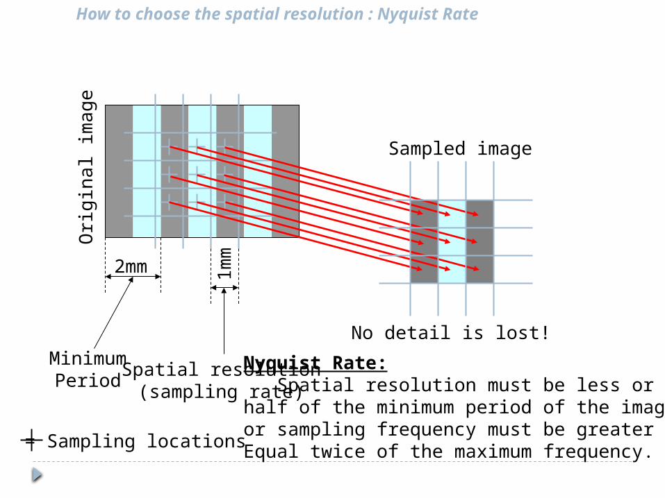
How to choose the spatial resolution : Nyquist Rate
Orig
inal
imag
e
= Sampling locations
MinimumPeriod Spatial resolution
(sampling rate)
Sampled image
No detail is lost!Nyquist Rate: Spatial resolution must be less or equalhalf of the minimum period of the imageor sampling frequency must be greater orEqual twice of the maximum frequency.
2mm 1mm
0 0.5 1 1.5 2-1
-0.5
0
0.5
1
0 0.5 1 1.5 2-1
-0.5
0
0.5
1
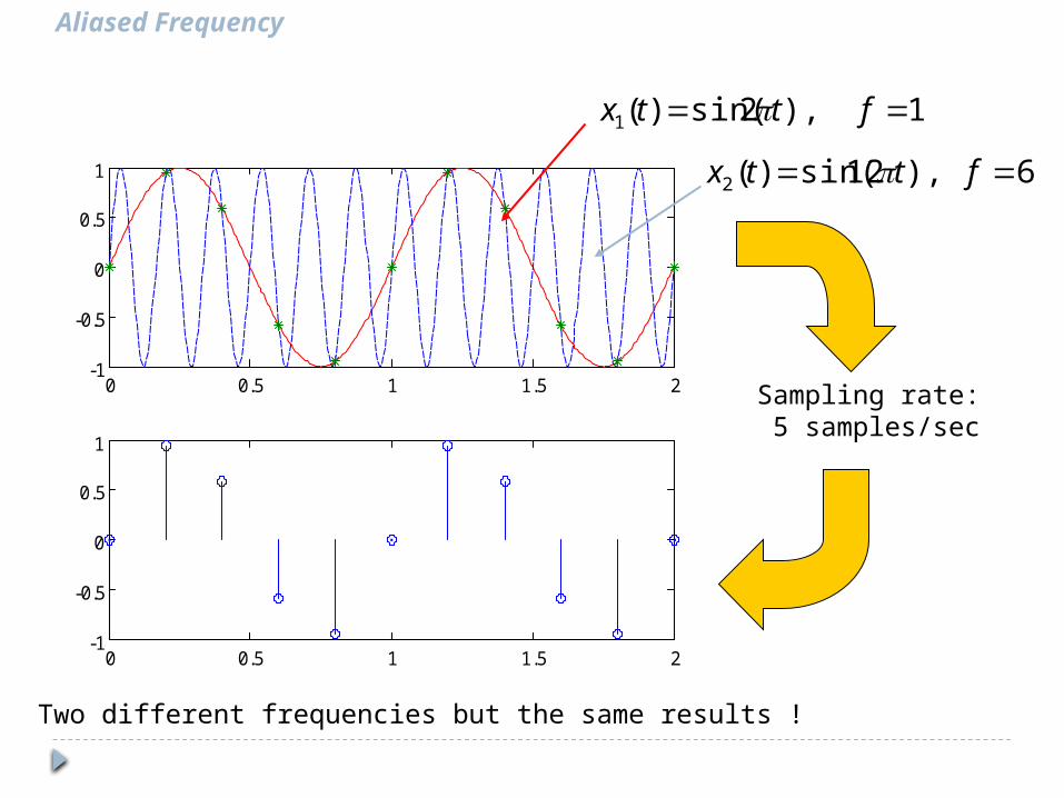
1 ),2sin()(1 fttx
6 ),12sin()(2 fttx
Sampling rate: 5 samples/sec
Aliased Frequency
Two different frequencies but the same results !
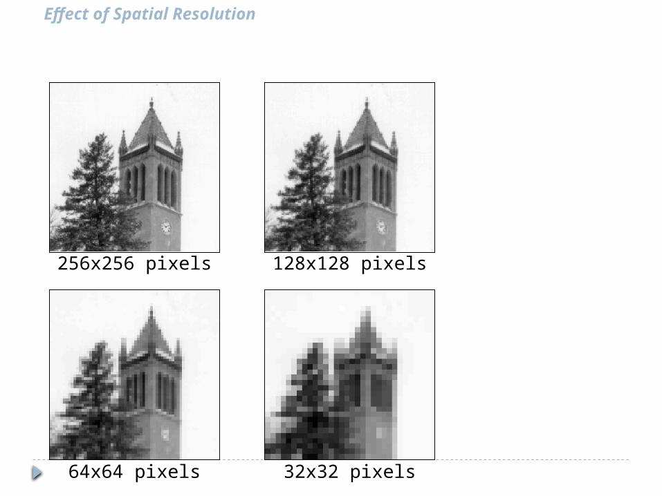
Effect of Spatial Resolution
256x256 pixels
64x64 pixels
128x128 pixels
32x32 pixels
Spatial Resolution It is a measure of the smallest discernible
detail in an image Can be stated in line pairs per unit distance,
and dots(pixels) per unit distance Dots per unit distance commonly used in
printing and publishing industry (dots per inch)
Newspaper are printed with a resolution of 75 dpi, magazines at 133 dpi, and glossy brochures at175 dpi
examples
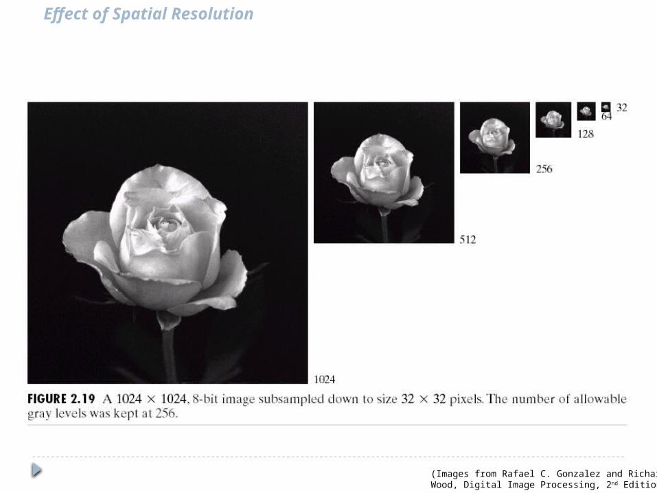
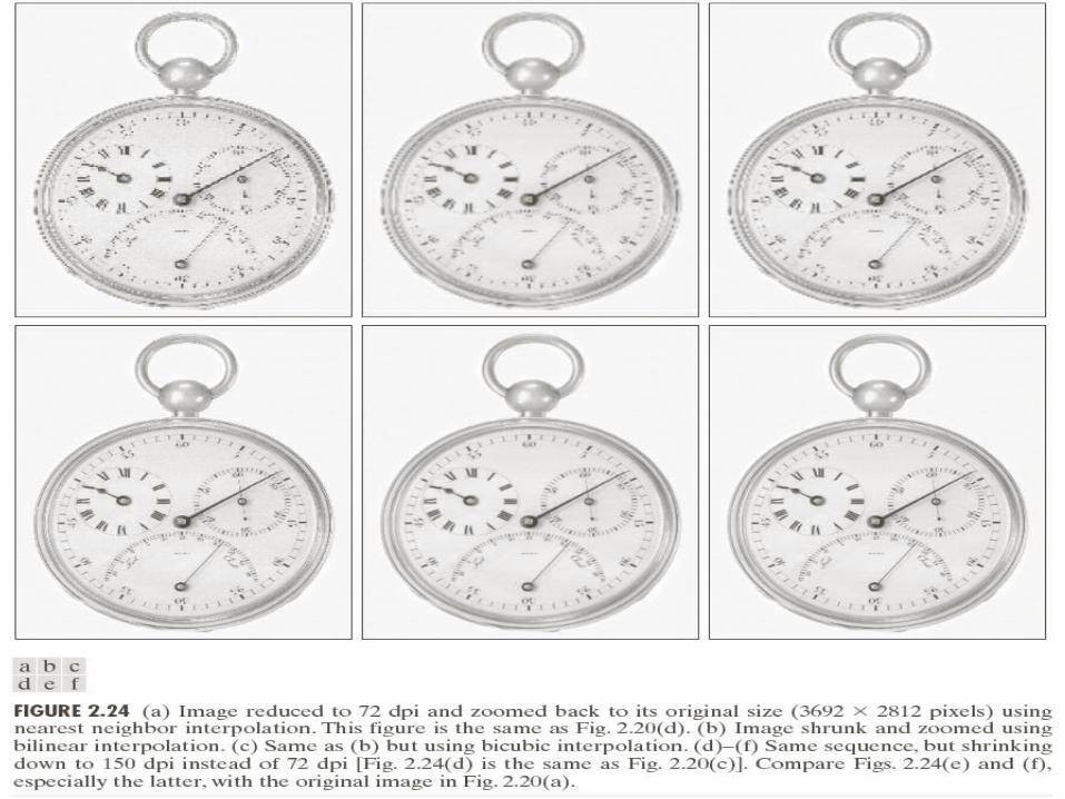
Effect of Spatial Resolution
(Images from Rafael C. Gonzalez and Richard E. Wood, Digital Image Processing, 2nd Edition.
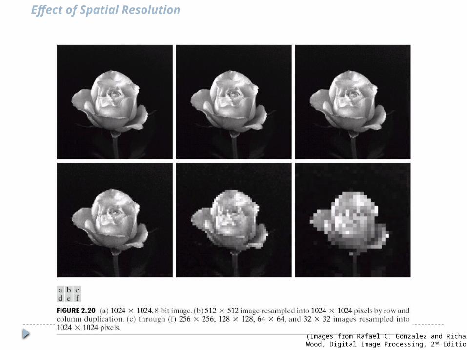
Effect of Spatial Resolution
(Images from Rafael C. Gonzalez and Richard E. Wood, Digital Image Processing, 2nd Edition.
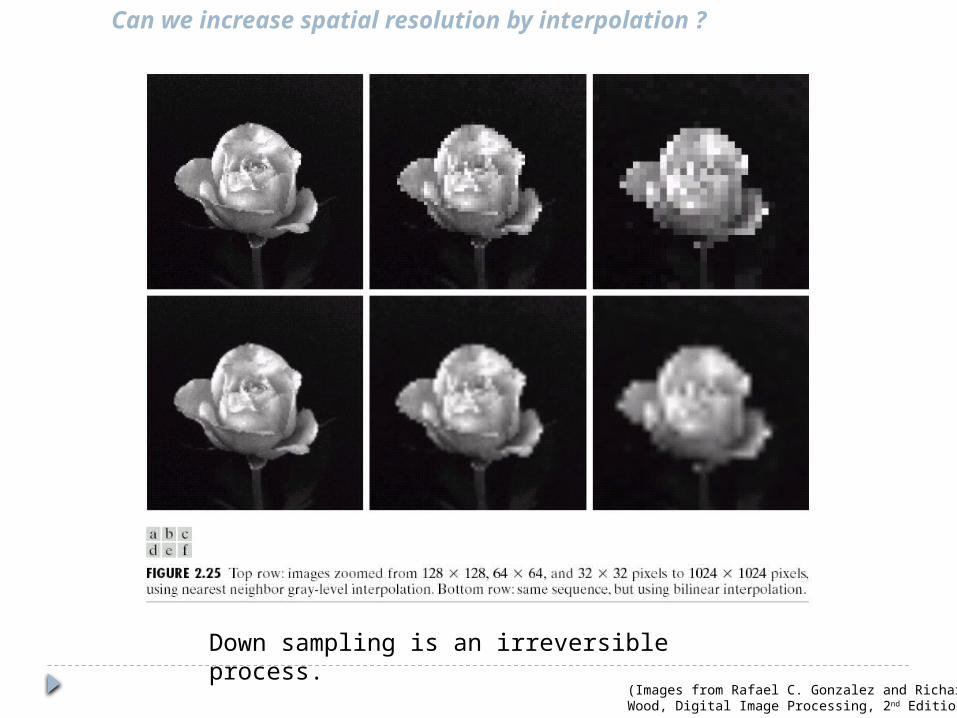
Can we increase spatial resolution by interpolation ?
Down sampling is an irreversible process.(Images from Rafael C. Gonzalez and Richard E. Wood, Digital Image Processing, 2nd Edition.
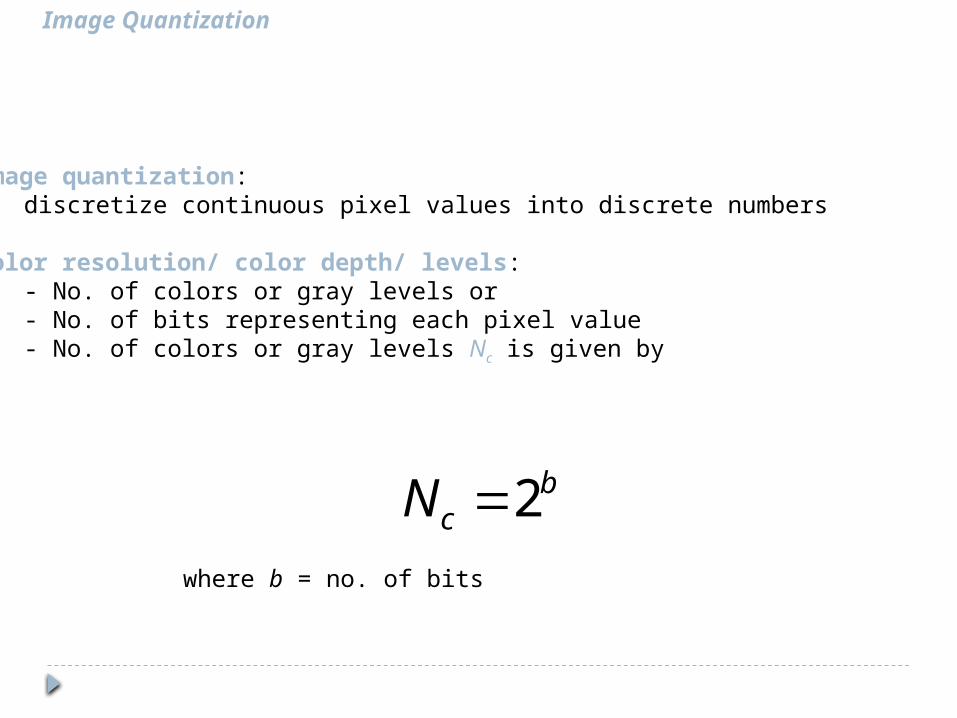
Image Quantization
Image quantization: discretize continuous pixel values into discrete numbers
Color resolution/ color depth/ levels: - No. of colors or gray levels or- No. of bits representing each pixel value- No. of colors or gray levels Nc is given by
bcN 2
where b = no. of bits
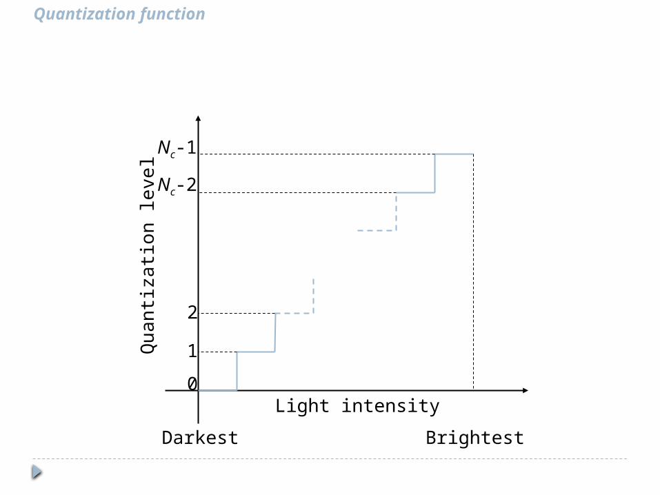
Quantization function
Light intensity
Quan
tizat
ion
leve
l
012
Nc-1Nc-2
Darkest Brightest
Intensity Resolution It refers to the smallest discernible change in
intensity level Number of intensity levels usually is an
integer power of two Also refers to Number of bits used to quantize
intensity as the intensity resolution Which intensity resolution is good for human
perception 8 bit, 16 bit, or 32 bit
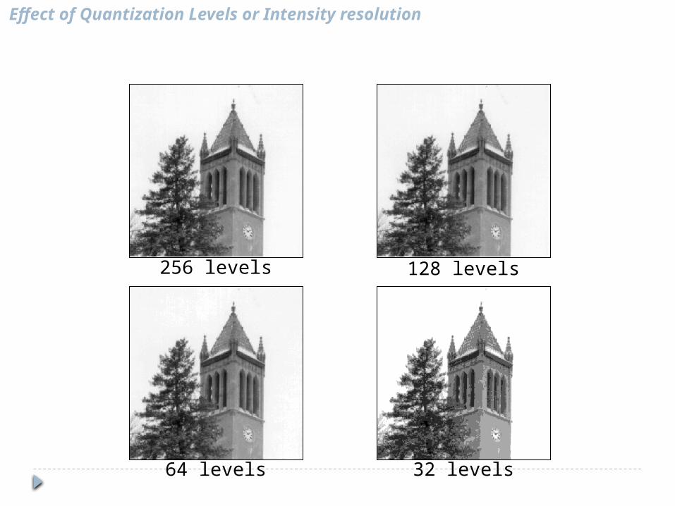
Effect of Quantization Levels or Intensity resolution
256 levels 128 levels
32 levels64 levels
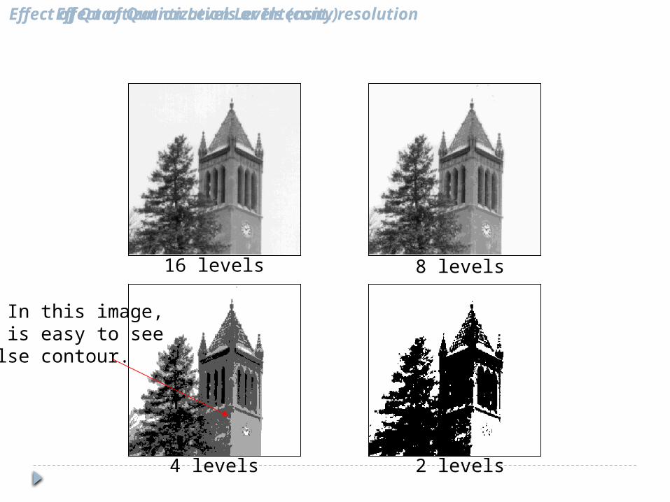
Effect of Quantization Levels (cont.)
16 levels 8 levels
2 levels4 levels
In this image,it is easy to seefalse contour.
Effect of Quantization Levels or Intensity resolution
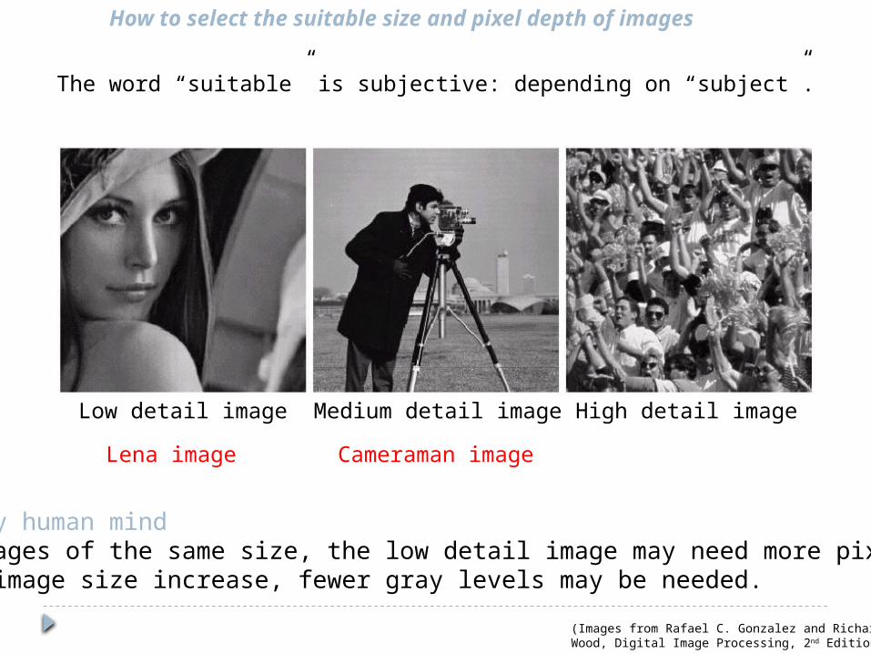
How to select the suitable size and pixel depth of images
Low detail image Medium detail image High detail imageLena image Cameraman image
To satisfy human mind1. For images of the same size, the low detail image may need more pixel depth.2. As an image size increase, fewer gray levels may be needed.
The word “suitable” is subjective: depending on “subject”.
(Images from Rafael C. Gonzalez and Richard E. Wood, Digital Image Processing, 2nd Edition.
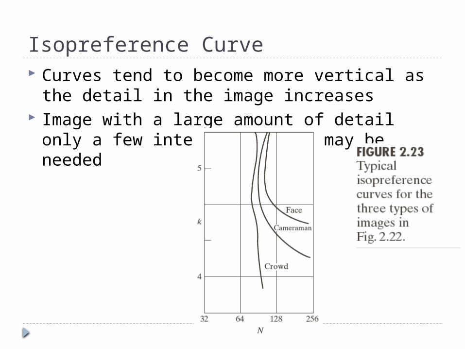
Isopreference Curve Curves tend to become more vertical as the
detail in the image increases Image with a large amount of detail only a few
intensity levels may be needed
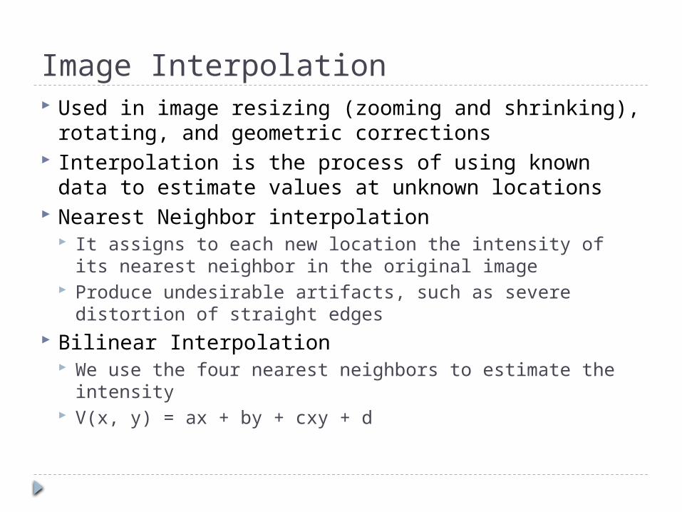
Image Interpolation Used in image resizing (zooming and shrinking),
rotating, and geometric corrections Interpolation is the process of using known data to
estimate values at unknown locations Nearest Neighbor interpolation
It assigns to each new location the intensity of its nearest neighbor in the original image
Produce undesirable artifacts, such as severe distortion of straight edges
Bilinear Interpolation We use the four nearest neighbors to estimate the
intensity V(x, y) = ax + by + cxy + d
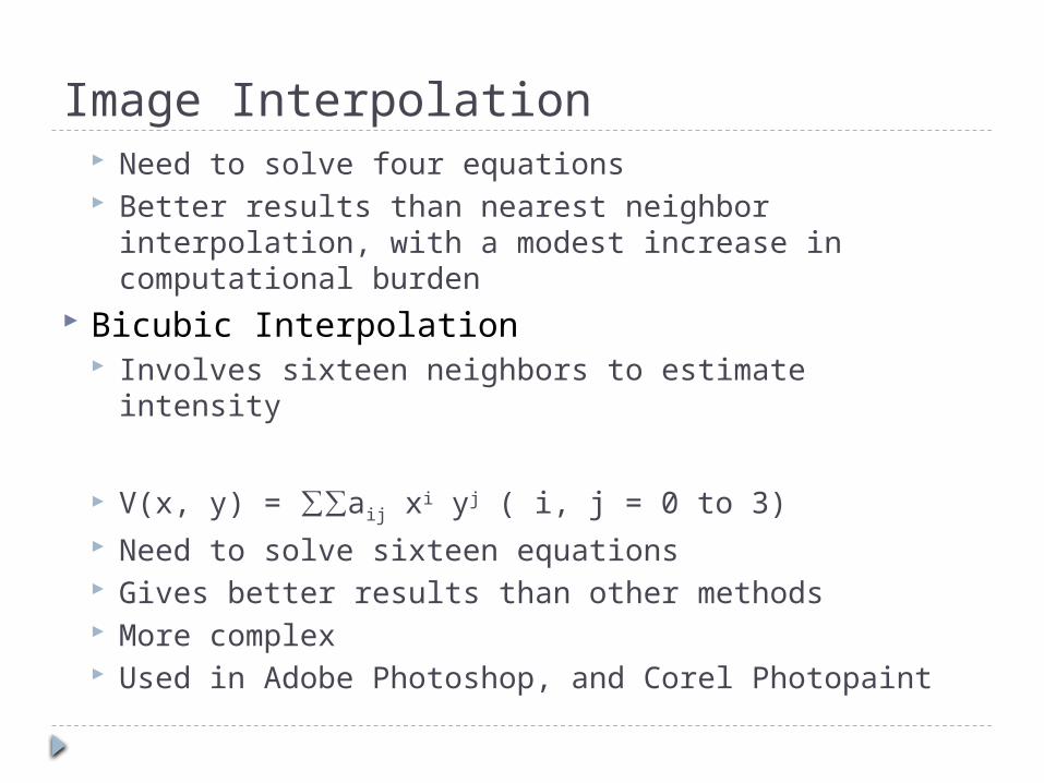
Image Interpolation Need to solve four equations Better results than nearest neighbor interpolation,
with a modest increase in computational burden Bicubic Interpolation
Involves sixteen neighbors to estimate intensity
V(x, y) = ∑∑aij xi yj ( i, j = 0 to 3) Need to solve sixteen equations Gives better results than other methods More complex Used in Adobe Photoshop, and Corel Photopaint
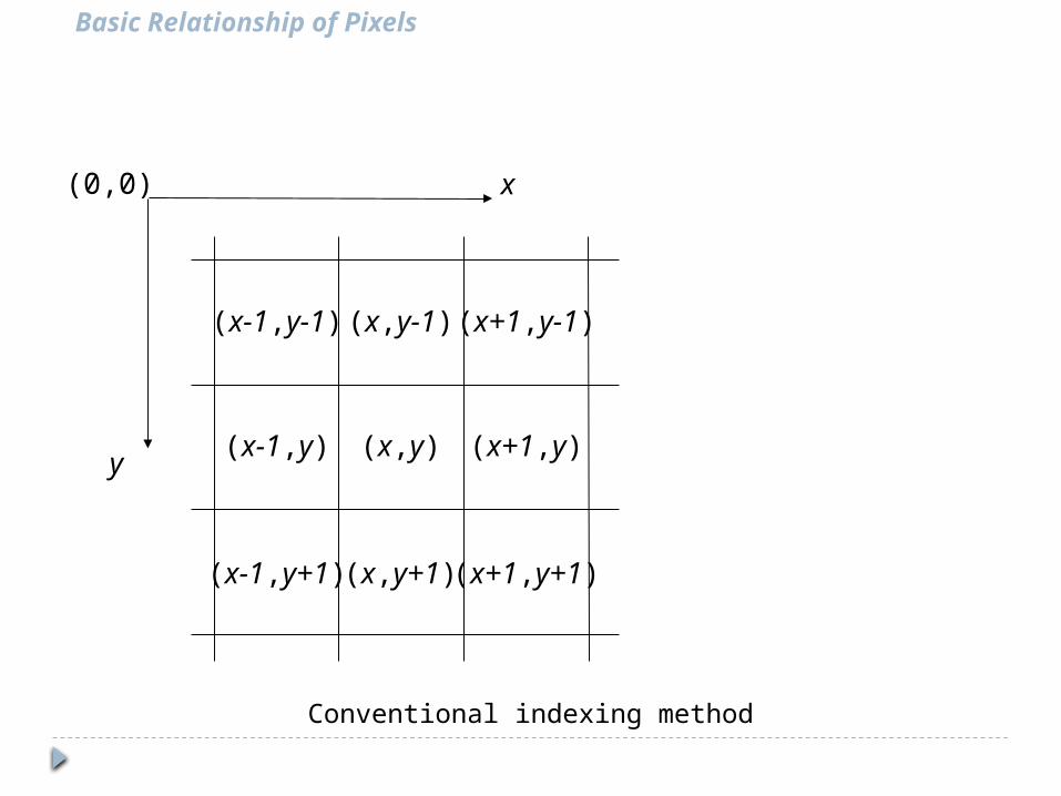
Basic Relationship of Pixels
x
y
(0,0)
Conventional indexing method
(x,y) (x+1,y)(x-1,y)
(x,y-1)
(x,y+1)
(x+1,y-1)(x-1,y-1)
(x-1,y+1) (x+1,y+1)
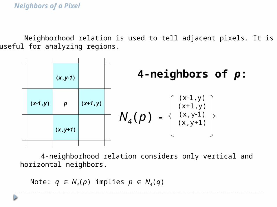
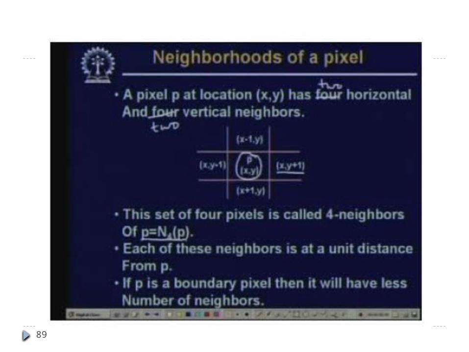
Neighbors of a Pixel
p (x+1,y)(x-1,y)
(x,y-1)
(x,y+1)
4-neighbors of p:
N4(p) =
(x-1,y)(x+1,y)(x,y-1)(x,y+1)
Neighborhood relation is used to tell adjacent pixels. It is useful for analyzing regions.
Note: q Î N4(p) implies p Î N4(q)
4-neighborhood relation considers only vertical and horizontal neighbors.
p (x+1,y)(x-1,y)
(x,y-1)
(x,y+1)
(x+1,y-1)(x-1,y-1)
(x-1,y+1) (x+1,y+1)
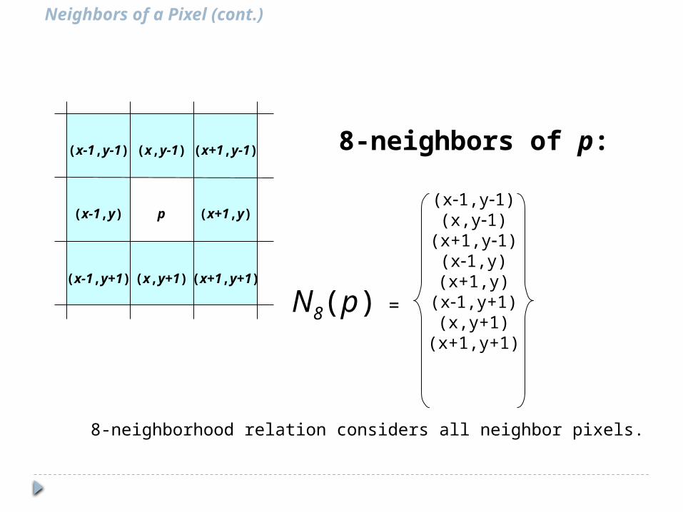
Neighbors of a Pixel (cont.)
8-neighbors of p:
(x-1,y-1)(x,y-1)
(x+1,y-1)(x-1,y)(x+1,y)
(x-1,y+1)(x,y+1)
(x+1,y+1)
N8(p) =
8-neighborhood relation considers all neighbor pixels.
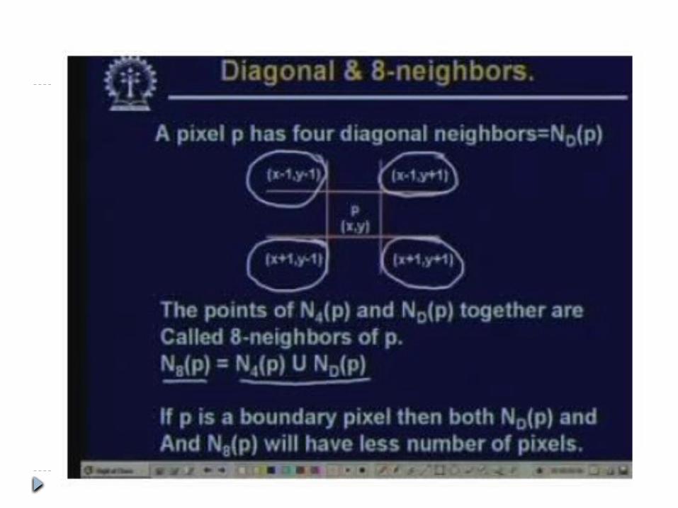
p
(x+1,y-1)(x-1,y-1)
(x-1,y+1) (x+1,y+1)
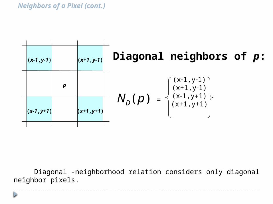
Diagonal neighbors of p:
ND(p) =
(x-1,y-1)(x+1,y-1)(x-1,y+1)
(x+1,y+1)
Neighbors of a Pixel (cont.)
Diagonal -neighborhood relation considers only diagonalneighbor pixels.
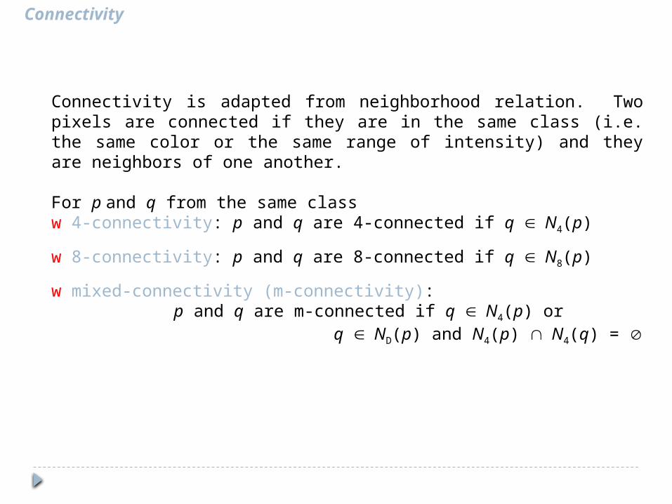
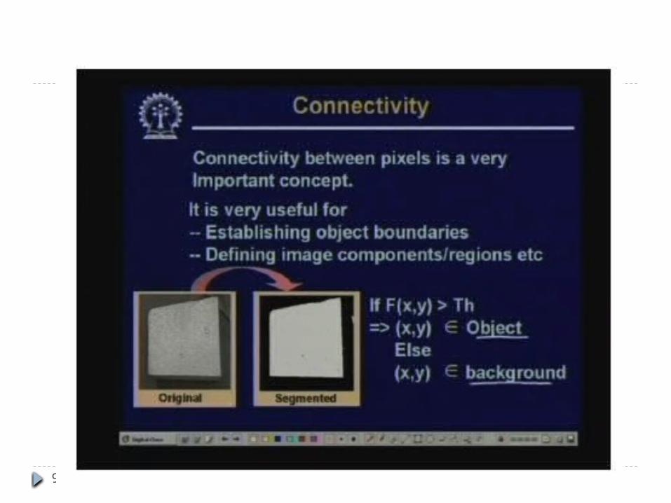
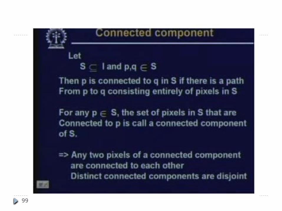
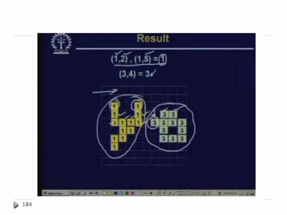
Connectivity
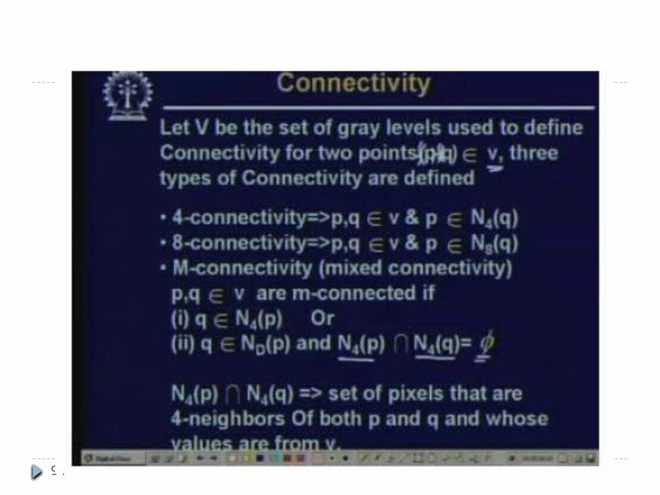
Connectivity is adapted from neighborhood relation. Two pixels are connected if they are in the same class (i.e. the same color or the same range of intensity) and they are neighbors of one another.
For p and q from the same classw 4-connectivity: p and q are 4-connected if q Î N4(p)w 8-connectivity: p and q are 8-connected if q Î N8(p)w mixed-connectivity (m-connectivity): p and q are m-connected if q Î N4(p) or q Î ND(p) and N4(p) Ç N4(q) = Æ
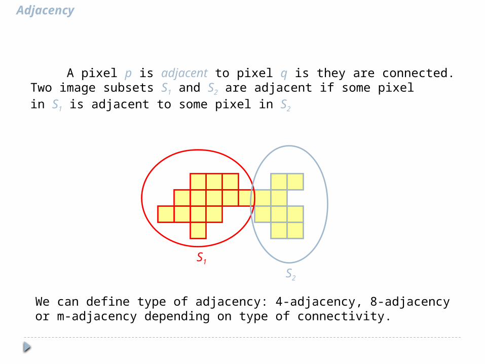
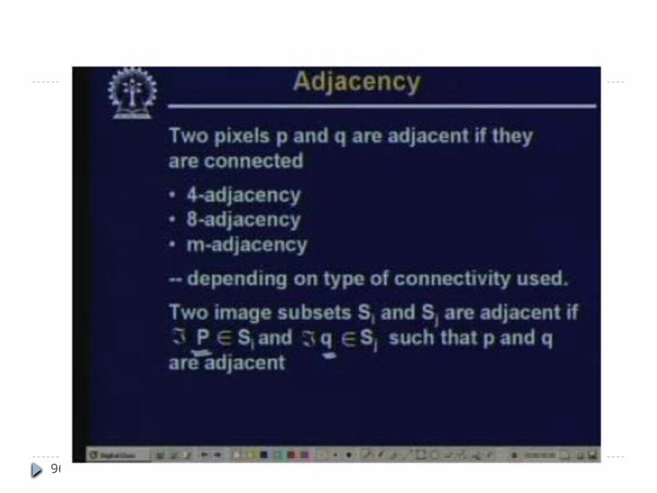
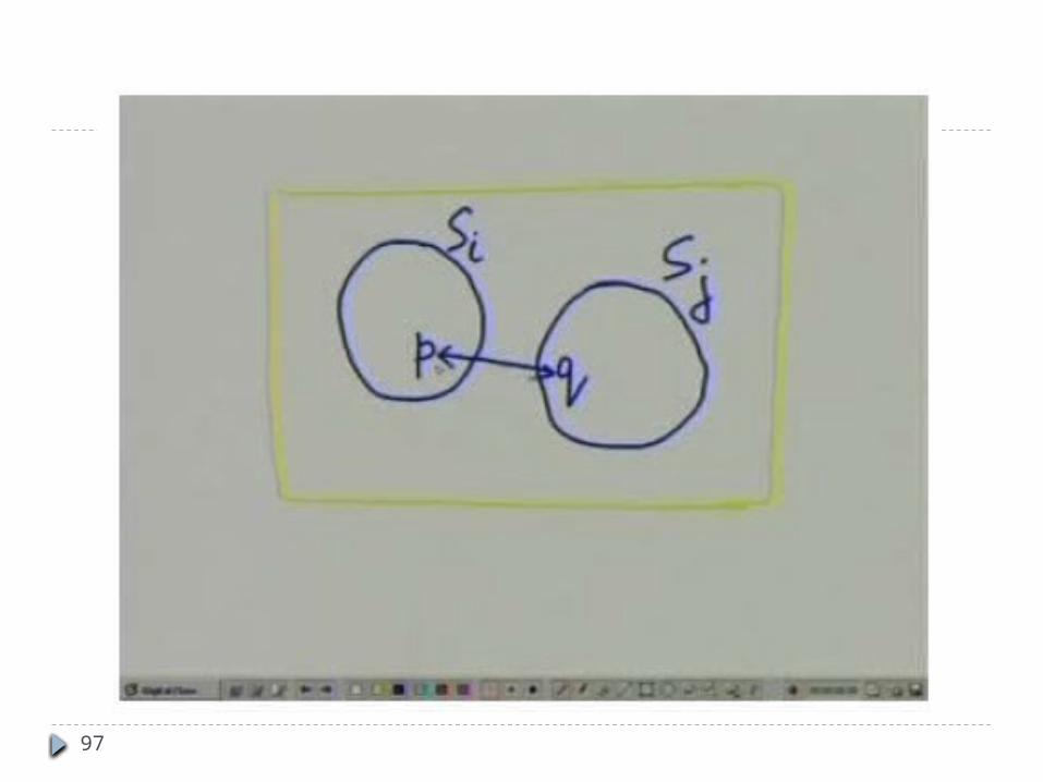
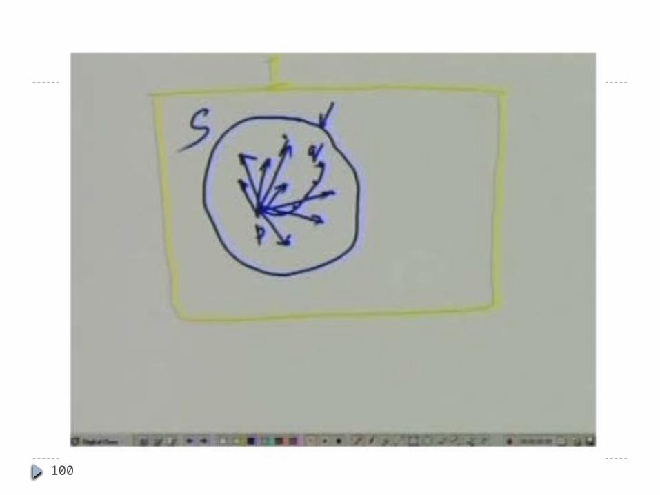
Adjacency
A pixel p is adjacent to pixel q is they are connected.Two image subsets S1 and S2 are adjacent if some pixelin S1 is adjacent to some pixel in S2
S1
S2
We can define type of adjacency: 4-adjacency, 8-adjacencyor m-adjacency depending on type of connectivity.
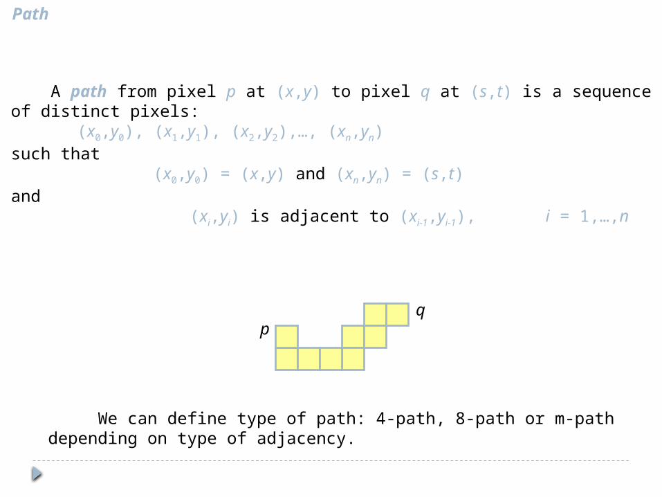
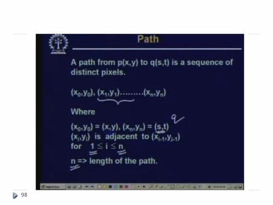
Path
A path from pixel p at (x,y) to pixel q at (s,t) is a sequenceof distinct pixels:
(x0,y0), (x1,y1), (x2,y2),…, (xn,yn)such that
(x0,y0) = (x,y) and (xn,yn) = (s,t)and (xi,yi) is adjacent to (xi-1,yi-1), i = 1,…,n
pq
We can define type of path: 4-path, 8-path or m-pathdepending on type of adjacency.
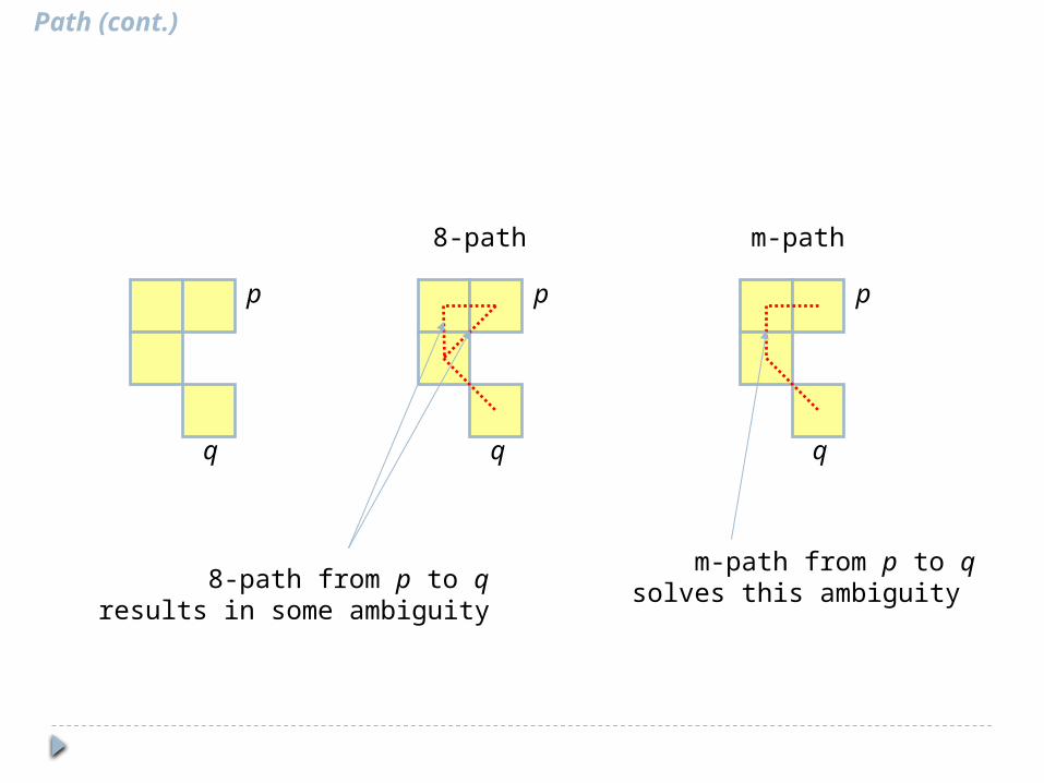
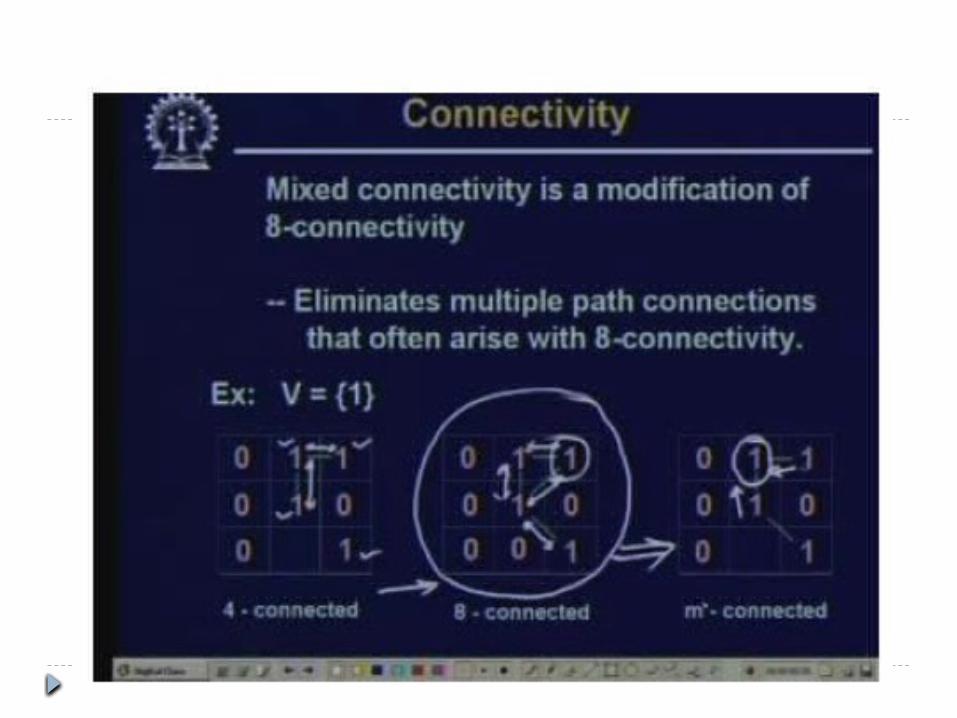
Path (cont.)
p
q
p
q
p
q
8-path from p to qresults in some ambiguity
m-path from p to qsolves this ambiguity
8-path m-path
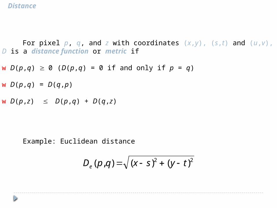
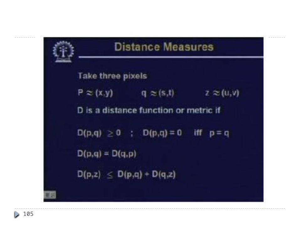
Distance
For pixel p, q, and z with coordinates (x,y), (s,t) and (u,v),D is a distance function or metric if
w D(p,q) ³ 0 (D(p,q) = 0 if and only if p = q)
w D(p,q) = D(q,p)
w D(p,z) £ D(p,q) + D(q,z)
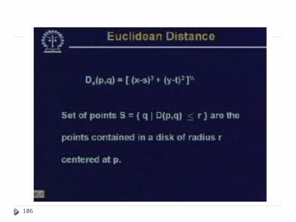
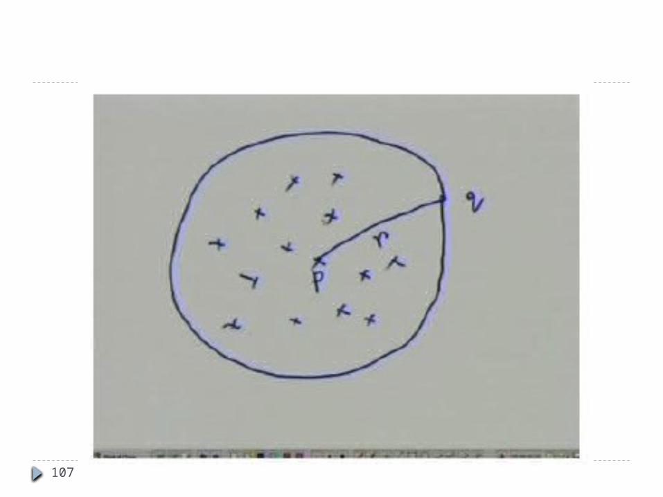
Example: Euclidean distance
22 )()(),( tysxqpDe -+-
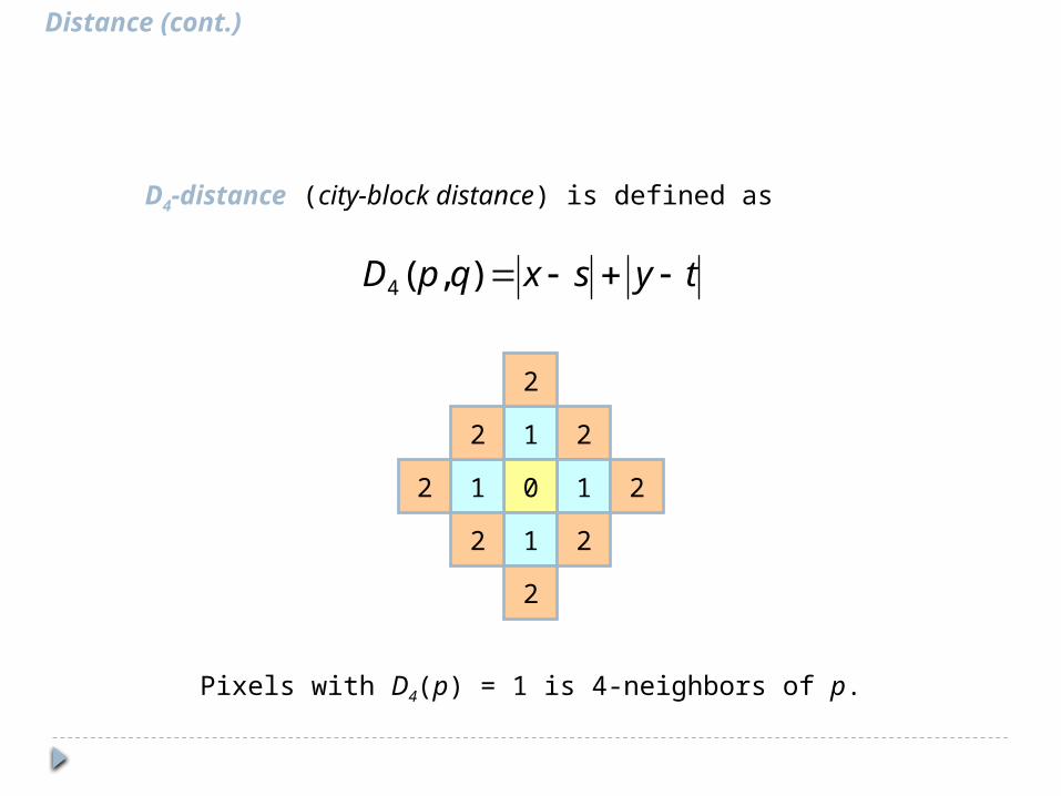
Distance (cont.)
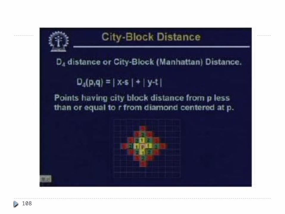
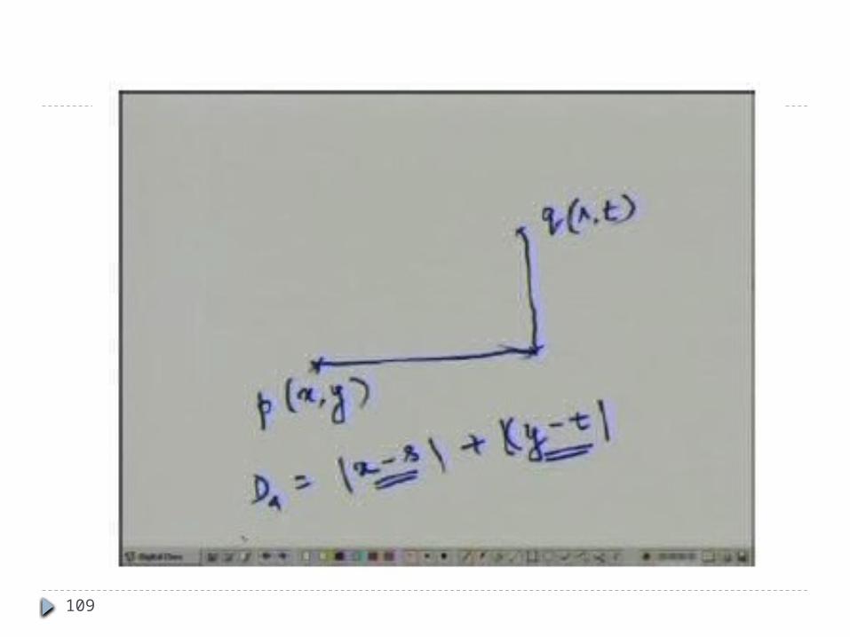
D4-distance (city-block distance) is defined as
tysxqpD -+-),(4
1 210
1 212
2
2
2
2
2
Pixels with D4(p) = 1 is 4-neighbors of p.
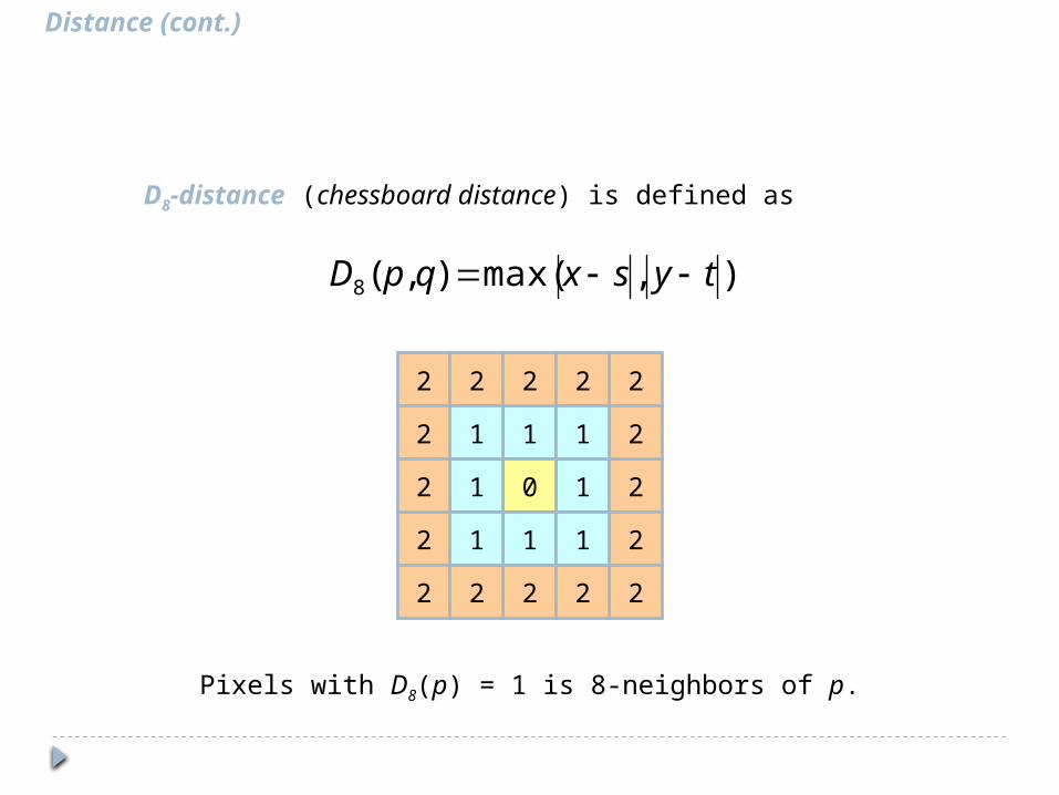
Distance (cont.)
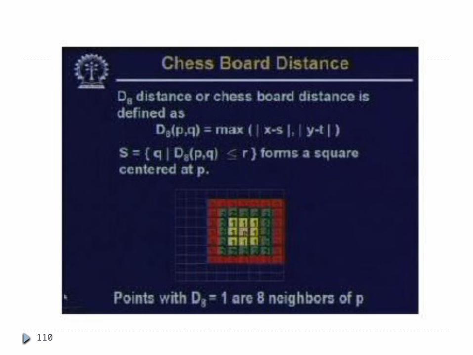
D8-distance (chessboard distance) is defined as
),max(),(8 tysxqpD --
12
101
2
12
2
2
2
2
2
Pixels with D8(p) = 1 is 8-neighbors of p.
22
2
2
2222
1
1
1
1
89
90
91
92

93
94
95
96
97
98
99
100
101
102
103
104
105
106
107
108
109
110
111
Boundary (Border or Contour)of a region R is the set of points that are adjacent to points in the complement of R.of a region is the set of pixels in the region that have at least one background neighbor.Inner BorderOuter Border
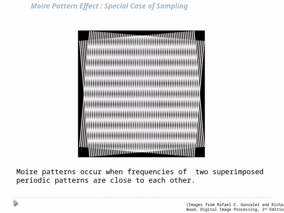
Moire Pattern Effect : Special Case of Sampling
Moire patterns occur when frequencies of two superimposed periodic patterns are close to each other.
(Images from Rafael C. Gonzalez and Richard E. Wood, Digital Image Processing, 2nd Edition.
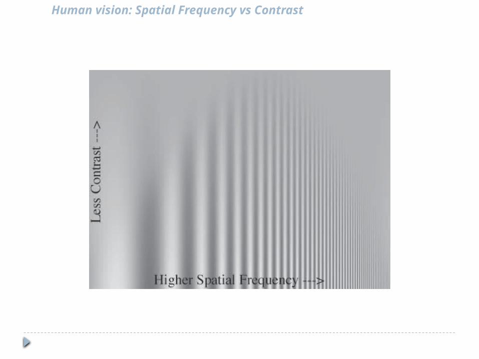
Human vision: Spatial Frequency vs Contrast
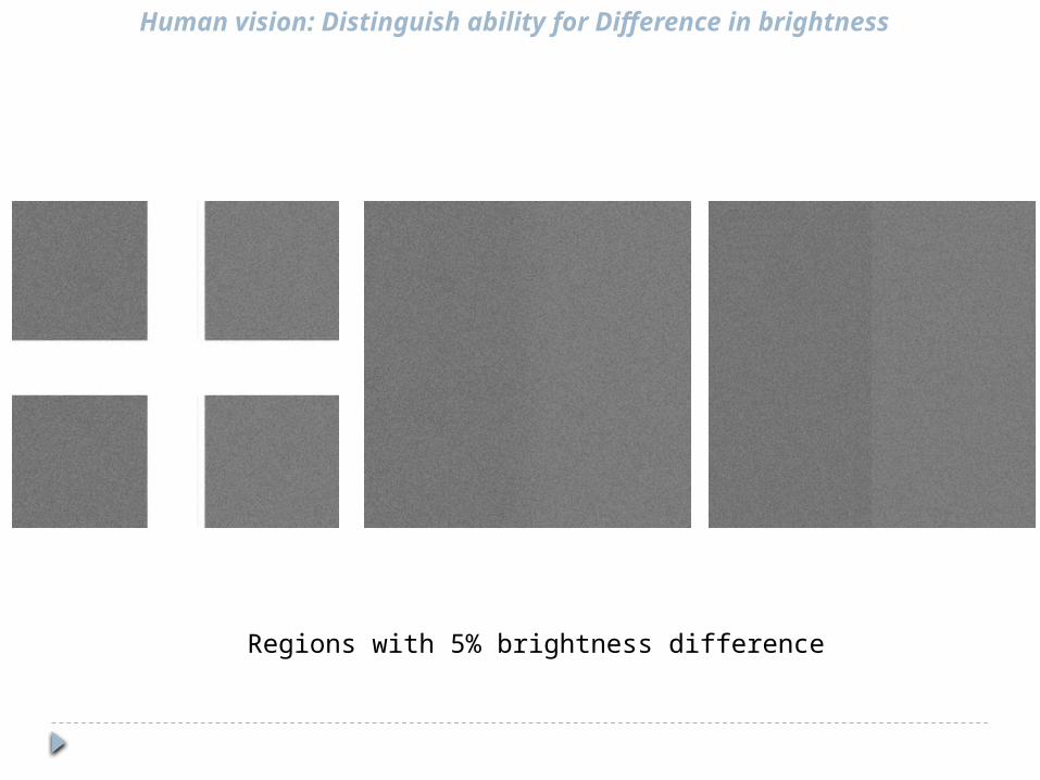
Human vision: Distinguish ability for Difference in brightness
Regions with 5% brightness difference