Embed Size (px)
Citation preview

P1: JZP0521840988pre CB1022/Xiong 0 521 84098 8 January 10, 2006 15:7
ii
This page intentionally left blank
P1: JZP0521840988pre CB1022/Xiong 0 521 84098 8 January 10, 2006 15:7
ESSENTIAL BIOINFORMATICS
Essential Bioinformatics is a concise yet comprehensive textbook of bioinformatics that
provides a broad introduction to the entire field. Written specifically for a life science
audience, the basics of bioinformatics are explained, followed by discussions of the state-
of-the-art computational tools available to solve biological research problems. All key areas
of bioinformatics are covered including biological databases, sequence alignment, gene
and promoter prediction, molecular phylogenetics, structural bioinformatics, genomics,
and proteomics. The book emphasizes how computational methods work and compares
the strengths and weaknesses of different methods. This balanced yet easily accessible text
will be invaluable to students who do not have sophisticated computational backgrounds.
Technical details of computational algorithms are explained with a minimum use of math-
ematical formulas; graphical illustrations are used in their place to aid understanding. The
effective synthesis of existing literature as well as in-depth and up-to-date coverage of all
key topics in bioinformatics make this an ideal textbook for all bioinformatics courses
taken by life science students and for researchers wishing to develop their knowledge of
bioinformatics to facilitate their own research.
Jin Xiong is an assistant professor of biology at Texas A&M University, where he has taught
bioinformatics to graduate and undergraduate students for several years. His main research
interest is in the experimental and bioinformatics analysis of photosystems.
i

P1: JZP0521840988pre CB1022/Xiong 0 521 84098 8 January 10, 2006 15:7
ii

P1: JZP0521840988pre CB1022/Xiong 0 521 84098 8 January 10, 2006 15:7
EssentialBioinformatics
JIN XIONGTexas A&M University
iii
cambridge university pressCambridge, New York, Melbourne, Madrid, Cape Town, Singapore, São Paulo
Cambridge University PressThe Edinburgh Building, Cambridge cb2 2ru, UK
First published in print format
isbn-13 978-0-521-84098-9
isbn-13 978-0-521-60082-8
isbn-13 978-0-511-16815-4
© Jin Xiong 2006
2006
Information on this title: www.cambridge.org/9780521840989
This publication is in copyright. Subject to statutory exception and to the provision ofrelevant collective licensing agreements, no reproduction of any part may take placewithout the written permission of Cambridge University Press.
isbn-10 0-511-16815-2
isbn-10 0-521-84098-8
isbn-10 0-521-60082-0
Cambridge University Press has no responsibility for the persistence or accuracy of urlsfor external or third-party internet websites referred to in this publication, and does notguarantee that any content on such websites is, or will remain, accurate or appropriate.
Published in the United States of America by Cambridge University Press, New York
www.cambridge.org
hardback
eBook (EBL)
eBook (EBL)
hardback

P1: JZP0521840988pre CB1022/Xiong 0 521 84098 8 January 10, 2006 15:7
Contents
Preface ■ ix
SECTION I INTRODUCTION AND BIOLOGICAL DATABASES
1 Introduction ■ 3What Is Bioinformatics? ■ 4Goal ■ 5Scope ■ 5Applications ■ 6Limitations ■ 7New Themes ■ 8Further Reading ■ 8
2 Introduction to Biological Databases ■ 10What Is a Database? ■ 10Types of Databases ■ 10Biological Databases ■ 13Pitfalls of Biological Databases ■ 17Information Retrieval from Biological Databases ■ 18Summary ■ 27Further Reading ■ 27
SECTION II SEQUENCE ALIGNMENT
3 Pairwise Sequence Alignment ■ 31Evolutionary Basis ■ 31Sequence Homology versus Sequence Similarity ■ 32Sequence Similarity versus Sequence Identity ■ 33Methods ■ 34Scoring Matrices ■ 41Statistical Significance of Sequence Alignment ■ 47Summary ■ 48Further Reading ■ 49
4 Database Similarity Searching ■ 51Unique Requirements of Database Searching ■ 51Heuristic Database Searching ■ 52Basic Local Alignment Search Tool (BLAST) ■ 52FASTA ■ 57Comparison of FASTA and BLAST ■ 60Database Searching with the Smith–Waterman Method ■ 61
v
P1: JZP0521840988pre CB1022/Xiong 0 521 84098 8 January 10, 2006 15:7
vi CONTENTS
Summary ■ 61Further Reading ■ 62
5 Multiple Sequence Alignment ■ 63Scoring Function ■ 63Exhaustive Algorithms ■ 64Heuristic Algorithms ■ 65Practical Issues ■ 71Summary ■ 73Further Reading ■ 74
6 Profiles and Hidden Markov Models ■ 75Position-Specific Scoring Matrices ■ 75Profiles ■ 77Markov Model and Hidden Markov Model ■ 79Summary ■ 84Further Reading ■ 84
7 Protein Motifs and Domain Prediction ■ 85Identification of Motifs and Domains in Multiple SequenceAlignment ■ 86Motif and Domain Databases Using Regular Expressions ■ 86Motif and Domain Databases Using Statistical Models ■ 87Protein Family Databases ■ 90Motif Discovery in Unaligned Sequences ■ 91Sequence Logos ■ 92Summary ■ 93Further Reading ■ 94
SECTION III GENE AND PROMOTER PREDICTION
8 Gene Prediction ■ 97Categories of Gene Prediction Programs ■ 97Gene Prediction in Prokaryotes ■ 98Gene Prediction in Eukaryotes ■ 103Summary ■ 111Further Reading ■ 111
9 Promoter and Regulatory Element Prediction ■ 113Promoter and Regulatory Elements in Prokaryotes ■ 113Promoter and Regulatory Elements in Eukaryotes ■ 114Prediction Algorithms ■ 115Summary ■ 123Further Reading ■ 124
SECTION IV MOLECULAR PHYLOGENETICS
10 Phylogenetics Basics ■ 127Molecular Evolution and Molecular Phylogenetics ■ 127Terminology ■ 128Gene Phylogeny versus Species Phylogeny ■ 130
P1: JZP0521840988pre CB1022/Xiong 0 521 84098 8 January 10, 2006 15:7
CONTENTS vii
Forms of Tree Representation ■ 131Why Finding a True Tree Is Difficult ■ 132Procedure ■ 133Summary ■ 140Further Reading ■ 141
11 Phylogenetic Tree Construction Methods and Programs ■ 142Distance-Based Methods ■ 142Character-Based Methods ■ 150Phylogenetic Tree Evaluation ■ 163Phylogenetic Programs ■ 167Summary ■ 168Further Reading ■ 169
SECTION V STRUCTURAL BIOINFORMATICS
12 Protein Structure Basics ■ 173Amino Acids ■ 173Peptide Formation ■ 174Dihedral Angles ■ 175Hierarchy ■ 176Secondary Structures ■ 178Tertiary Structures ■ 180Determination of Protein Three-Dimensional Structure ■ 181Protein Structure Database ■ 182Summary ■ 185Further Reading ■ 186
13 Protein Structure Visualization, Comparison,
and Classification ■ 187Protein Structural Visualization ■ 187Protein Structure Comparison ■ 190Protein Structure Classification ■ 195Summary ■ 199Further Reading ■ 199
14 Protein Secondary Structure Prediction ■ 200Secondary Structure Prediction for Globular Proteins ■ 201Secondary Structure Prediction for Transmembrane Proteins ■ 208Coiled Coil Prediction ■ 211Summary ■ 212Further Reading ■ 213
15 Protein Tertiary Structure Prediction ■ 214Methods ■ 215Homology Modeling ■ 215Threading and Fold Recognition ■ 223Ab Initio Protein Structural Prediction ■ 227CASP ■ 228Summary ■ 229Further Reading ■ 230
P1: JZP0521840988pre CB1022/Xiong 0 521 84098 8 January 10, 2006 15:7
viii CONTENTS
16 RNA Structure Prediction ■ 231Introduction ■ 231Types of RNA Structures ■ 233RNA Secondary Structure Prediction Methods ■ 234Ab Initio Approach ■ 234Comparative Approach ■ 237Performance Evaluation ■ 239Summary ■ 239Further Reading ■ 240
SECTION VI GENOMICS AND PROTEOMICS
17 Genome Mapping, Assembly, and Comparison ■ 243Genome Mapping ■ 243Genome Sequencing ■ 245Genome Sequence Assembly ■ 246Genome Annotation ■ 250Comparative Genomics ■ 255Summary ■ 259Further Reading ■ 259
18 Functional Genomics ■ 261Sequence-Based Approaches ■ 261Microarray-Based Approaches ■ 267Comparison of SAGE and DNA Microarrays ■ 278Summary ■ 279Further Reading ■ 280
19 Proteomics ■ 281Technology of Protein Expression Analysis ■ 281Posttranslational Modification ■ 287Protein Sorting ■ 289Protein–Protein Interactions ■ 291Summary ■ 296Further Reading ■ 296
APPENDIX
Appendix 1. Practical Exercises ■ 301
Appendix 2. Glossary ■ 318
Index ■ 331
P1: JZP0521840988pre CB1022/Xiong 0 521 84098 8 January 10, 2006 15:7
Preface
With a large number of prokaryotic and eukaryotic genomes completely sequencedand more forthcoming, access to the genomic information and synthesizing it forthe discovery of new knowledge have become central themes of modern biologicalresearch. Mining the genomic information requires the use of sophisticated com-putational tools. It therefore becomes imperative for the new generation of biol-ogists to be familiar with many bioinformatics programs and databases to tacklethe new challenges in the genomic era. To meet this goal, institutions in the UnitedStates and around the world are now offering graduate and undergraduate studentsbioinformatics-related courses to introduce them to relevant computational toolsnecessary for the genomic research. To support this important task, this text was writ-ten to provide comprehensive coverage on the state-of-the-art of bioinformatics in aclear and concise manner.
The idea of writing a bioinformatics textbook originated from my experience ofteaching bioinformatics at Texas A&M University. I needed a text that was compre-hensive enough to cover all major aspects in the field, technical enough for a college-level course, and sufficiently up to date to include most current algorithms while atthe same time being logical and easy to understand. The lack of such a comprehen-sive text at that time motivated me to write extensive lecture notes that attempted toalleviate the problem. The notes turned out to be very popular among the studentsand were in great demand from those who did not even take the class. To benefit alarger audience, I decided to assemble my lecture notes, as well as my experience andinterpretation of bioinformatics, into a book.
This book is aimed at graduate and undergraduate students in biology, or any prac-ticing molecular biologist, who has no background in computer algorithms but wishesto understand the fundamental principles of bioinformatics and use this knowledgeto tackle his or her own research problems. It covers major databases and softwareprograms for genomic data analysis, with an emphasis on the theoretical basis andpractical applications of these computational tools. By reading this book, the readerwill become familiar with various computational possibilities for modern molecularbiological research and also become aware of the strengths and weaknesses of eachof the software tools.
The reader is assumed to have a basic understanding of molecular biology and bio-chemistry. Therefore, many biological terms, such as nucleic acids, amino acids, genes,transcription, and translation, are used without further explanation. One exception isprotein structure, for which a chapter about fundamental concepts is included so that
ix

P1: JZP0521840988pre CB1022/Xiong 0 521 84098 8 January 10, 2006 15:7
x PREFACE
algorithms and rationales for protein structural bioinformatics can be better under-stood. Prior knowledge of advanced statistics, probability theories, and calculus is ofcourse preferable but not essential.
This book is organized into six sections: biological databases, sequence alignment,genes and promoter prediction, molecular phylogenetics, structural bioinformatics,and genomics and proteomics. There are nineteen chapters in total, each of whichis relatively independent. When information from one chapter is needed for under-standing another, cross-references are provided. Each chapter includes definitionsand key concepts as well as solutions to related computational problems. Occasion-ally there are boxes that show worked examples for certain types of calculations. Sincethis book is primarily for molecular biologists, very few mathematical formulas areused. A small number of carefully chosen formulas are used where they are abso-lutely necessary to understand a particular concept. The background discussion ofa computational problem is often followed by an introduction to related computerprograms that are available online. A summary is also provided at the end of eachchapter.
Most of the programs described in this book are online tools that are freely availableand do not require special expertise to use them. Most of them are rather straightfor-ward to use in that the user only needs to supply sequences or structures as input,and the results are returned automatically. In many cases, knowing which programsare available for which purposes is sufficient, though occasionally skills of interpret-ing the results are needed. However, in a number of instances, knowing the namesof the programs and their applications is only half the journey. The user also has tomake special efforts to learn the intricacies of using the programs. These programsare considered to be on the other extreme of user-friendliness. However, it would beimpractical for this book to try to be a computer manual for every available softwareprogram. That is not my goal in writing the book. Nonetheless, having realized thedifficulties of beginners who are often unaware of or, more precisely, intimidated bythe numerous software programs available, I have designed a number of practical Webexercises with detailed step-by-step procedures that aim to serve as examples of thecorrect use of a combined set of bioinformatics tools for solving a particular problem.The exercises were originally written for use on a UNIX workstation. However, theycan be used, with slight modifications, on any operating systems with Internet access.
In the course of preparing this book, I consulted numerous original articles andbooks related to certain topics of bioinformatics. I apologize for not being able toacknowledge all of these sources because of space limitations in such an introductorytext. However, a small number of articles (mainly recent review articles) and booksrelated to the topics of each chapter are listed as “Further Reading” for those whowish to seek more specialized information on the topics. Regarding the inclusion ofcomputational programs, there are often a large number of programs available fora particular task. I apologize for any personal bias in the selection of the softwareprograms in the book.
P1: JZP0521840988pre CB1022/Xiong 0 521 84098 8 January 10, 2006 15:7
PREFACE xi
One of the challenges in writing this text was to cover sufficient technical back-ground of computational methods without extensive display of mathematical formu-las. I strived to maintain a balance between explaining algorithms and not gettinginto too much mathematical detail, which may be intimidating for beginning stu-dents and nonexperts in computational biology. This sometimes proved to be a toughbalance for me because I risk either sacrificing some of the original content or losingthe reader. To alleviate this problem, I chose in many instances to use graphics insteadof formulas to illustrate a concept and to aid understanding.
I would like to thank the Department of Biology at Texas A&M University for theopportunity of letting me teach a bioinformatics class, which is what made this bookpossible. I thank all my friends and colleagues in the Department of Biology andthe Department of Biochemistry for their friendship. Some of my colleagues werekind enough to let me participate in their research projects, which provided me withdiverse research problems with which I could hone my bioinformatics analysis skills.I am especially grateful to Lisa Peres of the Molecular Simulation Laboratory at TexasA&M, who was instrumental in helping me set up and run the laboratory sectionof my bioinformatics course. I am also indebted to my former postdoctoral mentor,Carl Bauer of Indiana University, who gave me the wonderful opportunity to learnevolution and phylogenetics in great depth, which essentially launched my career inbioinformatics. Also importantly, I would like to thank Katrina Halliday, my editorat Cambridge University Press, for accepting the manuscript and providing numer-ous suggestions for polishing the early draft. It was a great pleasure working withher. Thanks also go to Cindy Fullerton and Marielle Poss for their diligent efforts inoverseeing the copyediting of the book to ensure a quality final product.
Jin Xiong

P1: JZP0521840988pre CB1022/Xiong 0 521 84098 8 January 10, 2006 15:7
xii

P1: JZP0521840988c01 CB1022/Xiong 0 521 84098 8 January 10, 2006 9:48
SECTION ONE
Introduction and Biological Databases
1

P1: JZP0521840988c01 CB1022/Xiong 0 521 84098 8 January 10, 2006 9:48
2
P1: JZP0521840988c01 CB1022/Xiong 0 521 84098 8 January 10, 2006 9:48
CHAPTER ONE
Introduction
Quantitation and quantitative tools are indispensable in modern biology. Most bio-logical research involves application of some type of mathematical, statistical, orcomputational tools to help synthesize recorded data and integrate various typesof information in the process of answering a particular biological question. For exam-ple, enumeration and statistics are required for assessing everyday laboratory exper-iments, such as making serial dilutions of a solution or counting bacterial colonies,phage plaques, or trees and animals in the natural environment. A classic example inthe history of genetics is by Gregor Mendel and Thomas Morgan, who, by simply count-ing genetic variations of plants and fruit flies, were able to discover the principles ofgenetic inheritance. More dedicated use of quantitative tools may involve using calcu-lus to predict the growth rate of a human population or to establish a kinetic model forenzyme catalysis. For very sophisticated uses of quantitative tools, one may find appli-cation of the “game theory” to model animal behavior and evolution, or the use of mil-lions of nonlinear partial differential equations to model cardiac blood flow. Whetherthe application is simple or complex, subtle or explicit, it is clear that mathemati-cal and computational tools have become an integral part of modern-day biologicalresearch. However, none of these examples of quantitative tool use in biology could beconsidered to be part of bioinformatics, which is also quantitative in nature. To help thereader understand the difference between bioinformatics and other elements of quan-titative biology, we provide a detailed explanation of what is bioinformatics in thefollowing sections.
Bioinformatics, which will be more clearly defined below, is the discipline of quan-titative analysis of information relating to biological macromolecules with the aid ofcomputers. The development of bioinformatics as a field is the result of advances inboth molecular biology and computer science over the past 30–40 years. Althoughthese developments are not described in detail here, understanding the history of thisdiscipline is helpful in obtaining a broader insight into current bioinformatics re-search. A succinct chronological summary of the landmark events that have had majorimpacts on the development of bioinformatics is presented here to provide context.
The earliest bioinformatics efforts can be traced back to the 1960s, although theword bioinformatics did not exist then. Probably, the first major bioinformatics projectwas undertaken by Margaret Dayhoff in 1965, who developed a first protein sequencedatabase called Atlas of Protein Sequence and Structure. Subsequently, in the early1970s, the Brookhaven National Laboratory established the Protein Data Bank forarchiving three-dimensional protein structures. At its onset, the database stored less
3
P1: JZP0521840988c01 CB1022/Xiong 0 521 84098 8 January 10, 2006 9:48
4 INTRODUCTION
than a dozen protein structures, compared to more than 30,000 structures today.The first sequence alignment algorithm was developed by Needleman and Wunschin 1970. This was a fundamental step in the development of the field of bioinfor-matics, which paved the way for the routine sequence comparisons and databasesearching practiced by modern biologists. The first protein structure prediction algo-rithm was developed by Chou and Fasman in 1974. Though it is rather rudimentary bytoday’s standard, it pioneered a series of developments in protein structure prediction.The 1980s saw the establishment of GenBank and the development of fast databasesearching algorithms such as FASTA by William Pearson and BLAST by StephenAltschul and coworkers. The start of the human genome project in the late 1980sprovided a major boost for the development of bioinformatics. The development andthe increasingly widespread use of the Internet in the 1990s made instant access to,and exchange and dissemination of, biological data possible.
These are only the major milestones in the establishment of this new field. Thefundamental reason that bioinformatics gained prominence as a discipline was theadvancement of genome studies that produced unprecedented amounts of biologicaldata. The explosion of genomic sequence information generated a sudden demandfor efficient computational tools to manage and analyze the data. The developmentof these computational tools depended on knowledge generated from a wide range ofdisciplines including mathematics, statistics, computer science, information technol-ogy, and molecular biology. The merger of these disciplines created an information-oriented field in biology, which is now known as bioinformatics.
WHAT IS BIOINFORMATICS?
Bioinformatics is an interdisciplinary research area at the interface between com-puter science and biological science. A variety of definitions exist in the literatureand on the world wide web; some are more inclusive than others. Here, we adopt thedefinition proposed by Luscombe et al. in defining bioinformatics as a union of biol-ogy and informatics: bioinformatics involves the technology that uses computers forstorage, retrieval, manipulation, and distribution of information related to biologicalmacromolecules such as DNA, RNA, and proteins. The emphasis here is on the use ofcomputers because most of the tasks in genomic data analysis are highly repetitive ormathematically complex. The use of computers is absolutely indispensable in mininggenomes for information gathering and knowledge building.
Bioinformatics differs from a related field known as computational biology. Bioin-formatics is limited to sequence, structural, and functional analysis of genes andgenomes and their corresponding products and is often considered computationalmolecular biology. However, computational biology encompasses all biological areasthat involve computation. For example, mathematical modeling of ecosystems, pop-ulation dynamics, application of the game theory in behavioral studies, and phylo-genetic construction using fossil records all employ computational tools, but do notnecessarily involve biological macromolecules.
P1: JZP0521840988c01 CB1022/Xiong 0 521 84098 8 January 10, 2006 9:48
SCOPE 5
Beside this distinction, it is worth noting that there are other views of how the twoterms relate. For example, one version defines bioinformatics as the development andapplication of computational tools in managing all kinds of biological data, whereascomputational biology is more confined to the theoretical development of algorithmsused for bioinformatics. The confusion at present over definition may partly reflectthe nature of this vibrant and quickly evolving new field.
GOALS
The ultimate goal of bioinformatics is to better understand a living cell and how itfunctions at the molecular level. By analyzing raw molecular sequence and structuraldata, bioinformatics research can generate new insights and provide a “global” per-spective of the cell. The reason that the functions of a cell can be better understoodby analyzing sequence data is ultimately because the flow of genetic information isdictated by the “central dogma” of biology in which DNA is transcribed to RNA, whichis translated to proteins. Cellular functions are mainly performed by proteins whosecapabilities are ultimately determined by their sequences. Therefore, solving func-tional problems using sequence and sometimes structural approaches has proved tobe a fruitful endeavor.
SCOPE
Bioinformatics consists of two subfields: the development of computational tools anddatabases and the application of these tools and databases in generating biologicalknowledge to better understand living systems. These two subfields are complemen-tary to each other. The tool development includes writing software for sequence,structural, and functional analysis, as well as the construction and curating of biolog-ical databases. These tools are used in three areas of genomic and molecular biologicalresearch: molecular sequence analysis, molecular structural analysis, and molecularfunctional analysis. The analyses of biological data often generate new problems andchallenges that in turn spur the development of new and better computational tools.
The areas of sequence analysis include sequence alignment, sequence databasesearching, motif and pattern discovery, gene and promoter finding, reconstruction ofevolutionary relationships, and genome assembly and comparison. Structural anal-yses include protein and nucleic acid structure analysis, comparison, classification,and prediction. The functional analyses include gene expression profiling, protein–protein interaction prediction, protein subcellular localization prediction, metabolicpathway reconstruction, and simulation (Fig. 1.1).
The three aspects of bioinformatics analysis are not isolated but often interactto produce integrated results (see Fig. 1.1). For example, protein structure predic-tion depends on sequence alignment data; clustering of gene expression profilesrequires the use of phylogenetic tree construction methods derived in sequenceanalysis. Sequence-based promoter prediction is related to functional analysis of

P1: JZP0521840988c01 CB1022/Xiong 0 521 84098 8 January 10, 2006 9:48
6 INTRODUCTION
Figure 1.1: Overview of various subfields of bioinformatics. Biocomputing tool development is at thefoundation of all bioinformatics analysis. The applications of the tools fall into three areas: sequenceanalysis, structure analysis, and function analysis. There are intrinsic connections between differentareas of analyses represented by bars between the boxes.
coexpressed genes. Gene annotation involves a number of activities, which includedistinction between coding and noncoding sequences, identification of translatedprotein sequences, and determination of the gene’s evolutionary relationship withother known genes; prediction of its cellular functions employs tools from all threegroups of the analyses.
APPLICATIONS
Bioinformatics has not only become essential for basic genomic and molecularbiology research, but is having a major impact on many areas of biotechnologyand biomedical sciences. It has applications, for example, in knowledge-based drugdesign, forensic DNA analysis, and agricultural biotechnology. Computational studiesof protein–ligand interactions provide a rational basis for the rapid identification ofnovel leads for synthetic drugs. Knowledge of the three-dimensional structures of pro-teins allows molecules to be designed that are capable of binding to the receptor siteof a target protein with great affinity and specificity. This informatics-based approach

P1: JZP0521840988c01 CB1022/Xiong 0 521 84098 8 January 10, 2006 9:48
LIMITATIONS 7
significantly reduces the time and cost necessary to develop drugs with higher potency,fewer side effects, and less toxicity than using the traditional trial-and-error approach.In forensics, results from molecular phylogenetic analysis have been accepted as evi-dence in criminal courts. Some sophisticated Bayesian statistics and likelihood-basedmethods for analysis of DNA have been applied in the analysis of forensic identity. Itis worth mentioning that genomics and bioinformtics are now poised to revolution-ize our healthcare system by developing personalized and customized medicine. Thehigh speed genomic sequencing coupled with sophisticated informatics technologywill allow a doctor in a clinic to quickly sequence a patient’s genome and easily detectpotential harmful mutations and to engage in early diagnosis and effective treatmentof diseases. Bioinformatics tools are being used in agriculture as well. Plant genomedatabases and gene expression profile analyses have played an important role in thedevelopment of new crop varieties that have higher productivity and more resistanceto disease.
LIMITATIONS
Having recognized the power of bioinformatics, it is also important to realize its lim-itations and avoid over-reliance on and over-expectation of bioinformatics output.In fact, bioinformatics has a number of inherent limitations. In many ways, the roleof bioinformatics in genomics and molecular biology research can be likened to therole of intelligence gathering in battlefields. Intelligence is clearly very important inleading to victory in a battlefield. Fighting a battle without intelligence is inefficientand dangerous. Having superior information and correct intelligence helps to identifythe enemy’s weaknesses and reveal the enemy’s strategy and intentions. The gatheredinformation can then be used in directing the forces to engage the enemy and winthe battle. However, completely relying on intelligence can also be dangerous if theintelligence is of limited accuracy. Overreliance on poor-quality intelligence can yieldcostly mistakes if not complete failures.
It is no stretch in analogy that fighting diseases or other biological problems usingbioinformatics is like fighting battles with intelligence. Bioinformatics and experimen-tal biology are independent, but complementary, activities. Bioinformatics dependson experimental science to produce raw data for analysis. It, in turn, provides usefulinterpretation of experimental data and important leads for further experimentalresearch. Bioinformatics predictions are not formal proofs of any concepts. Theydo not replace the traditional experimental research methods of actually testinghypotheses. In addition, the quality of bioinformatics predictions depends on thequality of data and the sophistication of the algorithms being used. Sequence datafrom high throughput analysis often contain errors. If the sequences are wrong orannotations incorrect, the results from the downstream analysis are misleading aswell. That is why it is so important to maintain a realistic perspective of the role ofbioinformatics.
P1: JZP0521840988c01 CB1022/Xiong 0 521 84098 8 January 10, 2006 9:48
8 INTRODUCTION
Bioinformatics is by no means a mature field. Most algorithms lack the capabil-ity and sophistication to truly reflect reality. They often make incorrect predictionsthat make no sense when placed in a biological context. Errors in sequence align-ment, for example, can affect the outcome of structural or phylogenetic analysis. Theoutcome of computation also depends on the computing power available. Manyaccurate but exhaustive algorithms cannot be used because of the slow rate of compu-tation. Instead, less accurate but faster algorithms have to be used. This is a necessarytrade-off between accuracy and computational feasibility. Therefore, it is importantto keep in mind the potential for errors produced by bioinformatics programs. Cautionshould always be exercised when interpreting prediction results. It is a good practiceto use multiple programs, if they are available, and perform multiple evaluations. Amore accurate prediction can often be obtained if one draws a consensus by compar-ing results from different algorithms.
NEW THEMES
Despite the pitfalls, there is no doubt that bioinformatics is a field that holds greatpotential for revolutionizing biological research in the coming decades. Currently, thefield is undergoing major expansion. In addition to providing more reliable and morerigorous computational tools for sequence, structural, and functional analysis, themajor challenge for future bioinformatics development is to develop tools for eluci-dation of the functions and interactions of all gene products in a cell. This presentsa tremendous challenge because it requires integration of disparate fields of biolog-ical knowledge and a variety of complex mathematical and statistical tools. To gaina deeper understanding of cellular functions, mathematical models are needed tosimulate a wide variety of intracellular reactions and interactions at the whole celllevel. This molecular simulation of all the cellular processes is termed systems biology.Achieving this goal will represent a major leap toward fully understanding a living sys-tem. That is why the system-level simulation and integration are considered the futureof bioinformatics. Modeling such complex networks and making predictions abouttheir behavior present tremendous challenges and opportunities for bioinformati-cians. The ultimate goal of this endeavor is to transform biology from a qualitativescience to a quantitative and predictive science. This is truly an exciting time forbioinformatics.
FURTHER READING
Attwood, T. K., and Miller, C. J. 2002. Progress in bioinformatics and the importance of beingearnest. Biotechnol. Annu. Rev. 8:1–54.
Golding, G. B. 2003. DNA and the revolution of molecular evolution, computational biology,and bioinformatics. Genome 46:930–5.
Goodman, N. 2002. Biological data becomes computer literature: New advances in bioinfor-matics. Curr. Opin. Biotechnol. 13:68–71.

P1: JZP0521840988c01 CB1022/Xiong 0 521 84098 8 January 10, 2006 9:48
FURTHER READING 9
Hagen. J. B. 2000. The origin of bioinformatics. Nat. Rev. Genetics 1:231–6.Kanehisa, M., and Bork, P. 2003. Bioinformatics in the post-sequence era. Nat. Genet. 33
Suppl:305–10.Kim, J. H. 2002. Bioinformatics and genomic medicine. Genet. Med. 4 Suppl:62S–5S.Luscombe, N. M., Greenbaum, D., and Gerstein, M. 2001. What is bioinformatics? A proposed
definition and overview of the field. Methods Inf. Med. 40:346–58.Ouzounis, C. A., and Valencia, A. 2003. Early bioinformatics: The birth of a discipline – A personal
view. Bioinformatics 19:2176–90.
P1: JZP0521840988c02 CB1022/Xiong 0 521 84098 8 January 10, 2006 14:42
CHAPTER TWO
Introduction to Biological Databases
One of the hallmarks of modern genomic research is the generation of enormousamounts of raw sequence data. As the volume of genomic data grows, sophisticatedcomputational methodologies are required to manage the data deluge. Thus, the veryfirst challenge in the genomics era is to store and handle the staggering volume of infor-mation through the establishment and use of computer databases. The developmentof databases to handle the vast amount of molecular biological data is thus a funda-mental task of bioinformatics. This chapter introduces some basic concepts related todatabases, in particular, the types, designs, and architectures of biological databases.Emphasis is on retrieving data from the main biological databases such as GenBank.
WHAT IS A DATABASE?
A database is a computerized archive used to store and organize data in such a waythat information can be retrieved easily via a variety of search criteria. Databasesare composed of computer hardware and software for data management. The chiefobjective of the development of a database is to organize data in a set of structuredrecords to enable easy retrieval of information. Each record, also called an entry,should contain a number of fields that hold the actual data items, for example, fieldsfor names, phone numbers, addresses, dates. To retrieve a particular record from thedatabase, a user can specify a particular piece of information, called value, to be foundin a particular field and expect the computer to retrieve the whole data record. Thisprocess is called making a query.
Although data retrieval is the main purpose of all databases, biological databasesoften have a higher level of requirement, known as knowledge discovery, which refersto the identification of connections between pieces of information that were notknown when the information was first entered. For example, databases containingraw sequence information can perform extra computational tasks to identify sequencehomology or conserved motifs. These features facilitate the discovery of new biologicalinsights from raw data.
TYPES OF DATABASES
Originally, databases all used a flat file format, which is a long text file that containsmany entries separated by a delimiter, a special character such as a vertical bar (|).Within each entry are a number of fields separated by tabs or commas. Except for the
10
P1: JZP0521840988c02 CB1022/Xiong 0 521 84098 8 January 10, 2006 14:42
TYPES OF DATABASES 11
raw values in each field, the entire text file does not contain any hidden instructionsfor computers to search for specific information or to create reports based on certainfields from each record. The text file can be considered a single table. Thus, to searcha flat file for a particular piece of information, a computer has to read through theentire file, an obviously inefficient process. This is manageable for a small database,but as database size increases or data types become more complex, this database stylecan become very difficult for information retrieval. Indeed, searches through such filesoften cause crashes of the entire computer system because of the memory-intensivenature of the operation.
To facilitate the access and retrieval of data, sophisticated computer softwareprograms for organizing, searching, and accessing data have been developed. Theyare called database management systems. These systems contain not only raw datarecords but also operational instructions to help identify hidden connections amongdata records. The purpose of establishing a data structure is for easy execution of thesearches and to combine different records to form final search reports. Dependingon the types of data structures,these database management systems can be classifiedinto two types: relational database management systems and object-oriented databasemanagement systems. Consequently, databases employing these management sys-tems are known as relational databases or object-oriented databases, respectively.
Relational Databases
Instead of using a single table as in a flat file database, relational databases use a setof tables to organize data. Each table, also called a relation, is made up of columnsand rows. Columns represent individual fields. Rows represent values in the fields ofrecords. The columns in a table are indexed according to a common feature calledan attribute, so they can be cross-referenced in other tables. To execute a query ina relational database, the system selects linked data items from different tables andcombines the information into one report. Therefore, specific information can befound more quickly from a relational database than from a flat file database.
Relational databases can be created using a special programming language calledstructured query language (SQL). The creation of this type of databases can take a greatdeal of planning during the design phase. After creation of the original database, anew data category can be easily added without requiring all existing tables to be mod-ified. The subsequent database searching and data gathering for reports are relativelystraightforward.
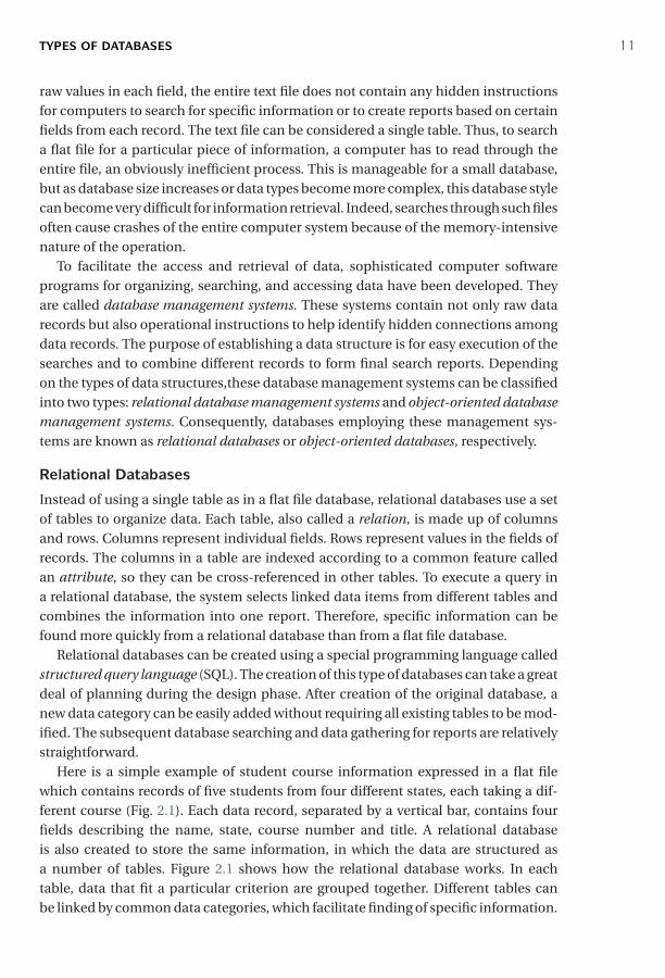
Here is a simple example of student course information expressed in a flat filewhich contains records of five students from four different states, each taking a dif-ferent course (Fig. 2.1). Each data record, separated by a vertical bar, contains fourfields describing the name, state, course number and title. A relational databaseis also created to store the same information, in which the data are structured asa number of tables. Figure 2.1 shows how the relational database works. In eachtable, data that fit a particular criterion are grouped together. Different tables canbe linked by common data categories, which facilitate finding of specific information.
P1: JZP0521840988c02 CB1022/Xiong 0 521 84098 8 January 10, 2006 14:42
12 INTRODUCTION TO BIOLOGICAL DATABASES
Figure 2.1: Example of constructing a relational database for five students’course information originallyexpressed in a flat file. By creating three different tables linked by common fields, data can be easilyaccessed and reassembled.
For example, if one is to ask the question, which courses are students from Texastaking? The database will first find the field for “State” in Table A and look up forTexas. This returns students 1 and 5. The student numbers are colisted in Table B,in which students 1 and 5 correspond to Biol 689 and Math 172, respectively. Thecourse names listed by course numbers are found in Table C. By going to Table C, exactcourse names corresponding to the course numbers can be retrieved. A final report isthen given showing that the Texans are taking the courses Bioinformatics and Calcu-lus. However, executing the same query through the flat file requires the computer toread through the entire text file word by word and to store the information in a tempo-ray memory space and later mark up the data records containing the word Texas. Thisis easily accomplishable for a small database. To perform queries in a large databaseusing flat files obviously becomes an onerous task for the computer system.
Object-Oriented Databases
One of the problems with relational databases is that the tables used do not describecomplex hierarchical relationships between data items. To overcome the problem,object-oriented databases have been developed that store data as objects. In anobject-oriented programming language, an object can be considered as a unit thatcombines data and mathematical routines that act on the data. The database is struc-tured such that the objects are linked by a set of pointers defining predetermined rela-tionships between the objects. Searching the database involves navigating through theobjects with the aid of the pointers linking different objects. Programming languageslike C++ are used to create object-oriented databases.
The object-oriented database system is more flexible; data can be structured basedon hierarchical relationships. By doing so, programming tasks can be simplified fordata that are known to have complex relationships, such as multimedia data. However,

P1: JZP0521840988c02 CB1022/Xiong 0 521 84098 8 January 10, 2006 14:42
BIOLOGICAL DATABASES 13
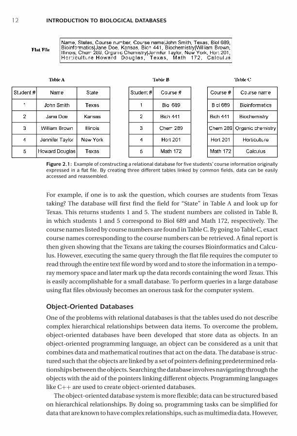
Figure 2.2: Example of construction and query of an object-oriented database using the same studentinformation as shown in Figure 2.1. Three objects are constructed and are linked by pointers shownas arrows. Finding specific information relies on navigating through the objects by way of pointers. Forsimplicity, some of the pointers are omitted.
this type of database system lacks the rigorous mathematical foundation of therelational databases. There is also a risk that some of the relationships between objectsmay be misrepresented. Some current databases have therefore incorporated featuresof both types of database programming, creating the object–relational database man-agement system.
The above students’ course information (Fig. 2.1) can be used to construct anobject-oriented database. Three different objects can be designed: student object,course object, and state object. Their interrelations are indicated by lines with arrows(Fig. 2.2). To answer the same question – which courses are students from Texastaking – one simply needs to start from Texas in the state object, which has pointersthat lead to students 1 and 5 in the student object. Further pointers in the studentobject point to the course each of the two students is taking. Therefore, a simplenavigation through the linked objects provides a final report.
BIOLOGICAL DATABASES
Current biological databases use all three types of database structures: flat files,relational, and object oriented. Despite the obvious drawbacks of using flat files indatabase management, many biological databases still use this format. The justifica-tion for this is that this system involves minimum amount of database design and thesearch output can be easily understood by working biologists.

P1: JZP0521840988c02 CB1022/Xiong 0 521 84098 8 January 10, 2006 14:42
14 INTRODUCTION TO BIOLOGICAL DATABASES
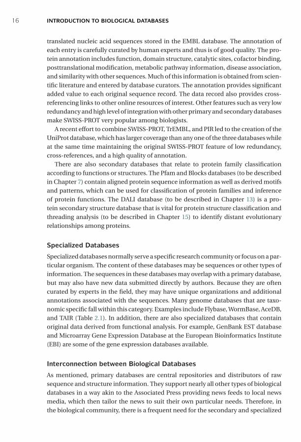
Based on their contents, biological databases can be roughly divided into threecategories: primary databases, secondary databases, and specialized databases.Primary databases contain original biological data. They are archives of raw sequenceor structural data submitted by the scientific community. GenBank and Protein DataBank (PDB) are examples of primary databases. Secondary databases contain com-putationally processed or manually curated information, based on original infor-mation from primary databases. Translated protein sequence databases containingfunctional annotation belong to this category. Examples are SWISS-Prot and Pro-tein Information Resources (PIR) (successor of Margaret Dayhoff’s Atlas of ProteinSequence and Structure [see Chapter 1]). Specialized databases are those that caterto a particular research interest. For example, Flybase, HIV sequence database, andRibosomal Database Project are databases that specialize in a particular organismor a particular type of data. A list of some frequently used databases is provided inTable 2.1.
Primary Databases
There are three major public sequence databases that store raw nucleic acid sequencedata produced and submitted by researchers worldwide: GenBank, the EuropeanMolecular Biology Laboratory (EMBL) database and the DNA Data Bank of Japan(DDBJ), which are all freely available on the Internet. Most of the data in the databasesare contributed directly by authors with a minimal level of annotation. A small numberof sequences, especially those published in the 1980s, were entered manually frompublished literature by database management staff.
Presently, sequence submission to either GenBank, EMBL, or DDBJ is a precondi-tion for publication in most scientific journals to ensure the fundamental moleculardata to be made freely available. These three public databases closely collaborateand exchange new data daily. They together constitute the International NucleotideSequence Database Collaboration. This means that by connecting to any one ofthe three databases, one should have access to the same nucleotide sequence data.Although the three databases all contain the same sets of raw data, each of the indi-vidual databases has a slightly different kind of format to represent the data.
Fortunately, for the three-dimensional structures of biological macromolecules,there is only one centralized database, the PDB. This database archives atomic coor-dinates of macromolecules (both proteins and nucleic acids) determined by x-raycrystallography and NMR. It uses a flat file format to represent protein name, authors,experimental details, secondary structure, cofactors, and atomic coordinates. Theweb interface of PDB also provides viewing tools for simple image manipulation.More details of this database and its format are provided in Chapter 12.
Secondary Databases
Sequence annotation information in the primary database is often minimal. Toturn the raw sequence information into more sophisticated biological knowledge,much postprocessing of the sequence information is needed. This begs the need for

P1: JZP0521840988c02 CB1022/Xiong 0 521 84098 8 January 10, 2006 14:42
BIOLOGICAL DATABASES 15
TABLE 2.1. Major Biological Databases Available Via the World Wide Web
Databases andRetrievalSystems Brief Summary of Content URL
AceDB Genome database forCaenorhabditis elegans
www.acedb.org
DDBJ Primary nucleotide sequencedatabase in Japan
www.ddbj.nig.ac.jp
EMBL Primary nucleotide sequencedatabase in Europe
www.ebi.ac.uk/embl/index.html
Entrez NCBI portal for a varietyof biological databases
www.ncbi.nlm.nih.gov/gquery/gquery.fcgi
ExPASY Proteomics database http://us.expasy.org/FlyBase A database of the Drosophila
genomehttp://flybase.bio.indiana.edu/
FSSP Protein secondary structures www.bioinfo.biocenter.helsinki.fi:8080/dali/index.htmlGenBank Primary nucleotide sequence
database in NCBIwww.ncbi.nlm.nih.gov/Genbank
HIV databases HIV sequence data and relatedimmunologic information
www.hiv.lanl.gov/content/index
Microarraygeneexpressiondatabase
DNA microarray data andanalysis tools
www.ebi.ac.uk/microarray
OMIM Genetic information of humandiseases
www.ncbi.nlm.nih.gov/entrez/query.fcgi?db=OMIM
PIR Annotated protein sequences http://pir.georgetown.edu/pirwww/pirhome3.shtmlPubMed Biomedical literature
informationwww.ncbi.nlm.nih.gov/PubMed
Ribosomaldatabaseproject
Ribosomal RNA sequences andphylogenetic trees derivedfrom the sequences
http://rdp.cme.msu.edu/html
SRS General sequence retrievalsystem
http://srs6.ebi.ac.uk
SWISS-Prot Curated protein sequencedatabase
www.ebi.ac.uk/swissprot/access.html
TAIR Arabidopsis informationdatabase
www.arabidopsis.org
secondary databases, which contain computationally processed sequence informa-tion derived from the primary databases. The amount of computational process-ing work varies greatly among the secondary databases; some are simple archives oftranslated sequence data from identified open reading frames in DNA, whereas othersprovide additional annotation and information related to higher levels of informationregarding structure and functions.
A prominent example of secondary databases is SWISS-PROT, which providesdetailed sequence annotation that includes structure, function, and protein fam-ily assignment. The sequence data are mainly derived from TrEMBL, a database of
P1: JZP0521840988c02 CB1022/Xiong 0 521 84098 8 January 10, 2006 14:42
16 INTRODUCTION TO BIOLOGICAL DATABASES
translated nucleic acid sequences stored in the EMBL database. The annotation ofeach entry is carefully curated by human experts and thus is of good quality. The pro-tein annotation includes function, domain structure, catalytic sites, cofactor binding,posttranslational modification, metabolic pathway information, disease association,and similarity with other sequences. Much of this information is obtained from scien-tific literature and entered by database curators. The annotation provides significantadded value to each original sequence record. The data record also provides cross-referencing links to other online resources of interest. Other features such as very lowredundancy and high level of integration with other primary and secondary databasesmake SWISS-PROT very popular among biologists.
A recent effort to combine SWISS-PROT, TrEMBL, and PIR led to the creation of theUniProt database, which has larger coverage than any one of the three databases whileat the same time maintaining the original SWISS-PROT feature of low redundancy,cross-references, and a high quality of annotation.
There are also secondary databases that relate to protein family classificationaccording to functions or structures. The Pfam and Blocks databases (to be describedin Chapter 7) contain aligned protein sequence information as well as derived motifsand patterns, which can be used for classification of protein families and inferenceof protein functions. The DALI database (to be described in Chapter 13) is a pro-tein secondary structure database that is vital for protein structure classification andthreading analysis (to be described in Chapter 15) to identify distant evolutionaryrelationships among proteins.
Specialized Databases
Specialized databases normally serve a specific research community or focus on a par-ticular organism. The content of these databases may be sequences or other types ofinformation. The sequences in these databases may overlap with a primary database,but may also have new data submitted directly by authors. Because they are oftencurated by experts in the field, they may have unique organizations and additionalannotations associated with the sequences. Many genome databases that are taxo-nomic specific fall within this category. Examples include Flybase, WormBase, AceDB,and TAIR (Table 2.1). In addition, there are also specialized databases that containoriginal data derived from functional analysis. For example, GenBank EST databaseand Microarray Gene Expression Database at the European Bioinformatics Institute(EBI) are some of the gene expression databases available.
Interconnection between Biological Databases
As mentioned, primary databases are central repositories and distributors of rawsequence and structure information. They support nearly all other types of biologicaldatabases in a way akin to the Associated Press providing news feeds to local newsmedia, which then tailor the news to suit their own particular needs. Therefore, inthe biological community, there is a frequent need for the secondary and specialized

P1: JZP0521840988c02 CB1022/Xiong 0 521 84098 8 January 10, 2006 14:42
PITFALLS OF BIOLOGICAL DATABASES 17
databases to connect to the primary databases and to keep uploading sequence infor-mation. In addition, a user often needs to get information from both primary and sec-ondary databases to complete a task because the information in a single database isoften insufficient. Instead of letting users visiting multiple databases, it is convenientfor entries in a database to be cross-referenced and linked to related entries in otherdatabases that contain additional information. All these create a demand for linkingdifferent databases.
The main barrier to linking different biological databases is format incompati-bility current biological databases utilize all three types of database structures – flatfiles, relational, and object oriented. The heterogeneous database structures limitcommunication between databases. One solution to networking the databases isto use a specification language called Common Object Request Broker Architecture(COBRA), which allows database programs at different locations to communicate ina network through an “interface broker” without having to understand each other’sdatabase structure. It works in a way similar to HyperText Markup Language (HTML)for web pages, labeling database entries using a set of common tags.
A similar protocol called eXtensible Markup Language (XML) also helps in bridgingdatabases. In this format, each biological record is broken down into small, basic com-ponents that are labeled with a hierarchical nesting of tags. This database structuresignificantly improves the distribution and exchange of complex sequence anno-tations between databases. Recently, a specialized protocol for bioinformatics dataexchange has been developed. It is the distributed annotation system, which allowsone computer to contact multiple servers and retrieve dispersed sequence annota-tion information related to a particular sequence and integrate the results into a singlecombined report.
PITFALLS OF BIOLOGICAL DATABASES
One of the problems associated with biological databases is overreliance onsequence information and related annotations, without understanding the reliabi-lity of the information. What is often ignored is the fact that there are many errors insequence databases. There are also high levels of redundancy in the primary sequencedatabases. Annotations of genes can also occasionally be false or incomplete. Allthese types of errors can be passed on to other databases, causing propagation oferrors.
Most errors in nucleotide sequences are caused by sequencing errors. Some ofthese errors cause frameshifts that make whole gene identification difficult or proteintranslation impossible. Sometimes, gene sequences are contaminated with sequencesfrom cloning vectors. Generally speaking, errors are more common for sequences pro-duced before the 1990s; sequence quality has been greatly improved since. Therefore,exceptional care should be taken when dealing with more dated sequences.
Redundancy is another major problem affecting primary databases. There istremendous duplication of information in the databases, for various reasons. The

P1: JZP0521840988c02 CB1022/Xiong 0 521 84098 8 January 10, 2006 14:42
18 INTRODUCTION TO BIOLOGICAL DATABASES
causes of redundancy include repeated submission of identical or overlappingsequences by the same or different authors, revision of annotations, dumping ofexpressed sequence tags (EST) data (see Chapter 18), and poor database managementthat fails to detect the redundancy. This makes some primary databases excessivelylarge and unwieldy for information retrieval.
Steps have been taken to reduce the redundancy. The National Center for Biotech-nology Information (NCBI) has now created a nonredundant database, called RefSeq,in which identical sequences from the same organism and associated sequence frag-ments are merged into a single entry. Proteins sequences derived from the sameDNA sequences are explicitly linked as related entries. Sequence variants from thesame organism with very minor differences, which may well be caused by sequencingerrors, are treated as distinctly related entries. This carefully curated database can beconsidered a secondary database.
As mentioned, the SWISS-PROT database also has minimal redundancy for proteinsequences compared to most other databases. Another way to address the redundancyproblem is to create sequence-cluster databases such as UniGene (see Chapter 18)that coalesce EST sequences that are derived from the same gene.
The other common problem is erroneous annotations. Often, the same genesequence is found under different names resulting in multiple entries and confu-sion about the data. Or conversely, unrelated genes bearing the same name are foundin the databases. To alleviate the problem of naming genes, reannotation of genes andproteins using a set of common, controlled vocabulary to describe a gene or proteinis necessary. The goal is to provide a consistent and unambiguous naming system forall genes and proteins. A prominent example of such systems is Gene Ontology (seeChapter 17).
Some of the inconsistencies in annotation could be caused by genuine disagree-ment between researchers in the field; others may result from imprudent assignmentof protein functions by sequence submitters. There are also some errors that are sim-ply caused by omissions or mistakes in typing. Errors in annotation can be particularlydamaging because the large majority of new sequences are assigned functions basedon similarity with sequences in the databases that are already annotated. Therefore, awrong annotation can be easily transferred to all similar genes in the entire database.It is possible that some of these errors can be corrected at the informatics level bystudying the protein domains and families. However, others eventually have to becorrected using experimental work.
INFORMATION RETRIEVAL FROM BIOLOGICAL DATABASES
As mentioned, a major goal in developing databases is to provide efficient and user-friendly access to the data stored. There are a number of retrieval systems for bio-logical data. The most popular retrieval systems for biological databases are Entrezand Sequence Retrieval Systems (SRS) that provide access to multiple databases forretrieval of integrated search results.
P1: JZP0521840988c02 CB1022/Xiong 0 521 84098 8 January 10, 2006 14:42
INFORMATION RETRIEVAL FROM BIOLOGICAL DATABASES 19
To perform complex queries in a database often requires the use of Boolean oper-ators. This is to join a series of keywords using logical terms such as AND, OR, andNOT to indicate relationships between the keywords used in a search. AND meansthat the search result must contain both words; OR means to search for results con-taining either word or both; NOT excludes results containing either one of the words.In addition, one can use parentheses ( ) to define a concept if multiple words andrelationships are involved, so that the computer knows which part of the search toexecute first. Items contained within parentheses are executed first. Quotes can beused to specify a phrase. Most search engines of public biological databases use someform of this Boolean logic.
Entrez
The NCBI developed and maintains Entrez, a biological database retrieval system.It is a gateway that allows text-based searches for a wide variety of data, includingannotated genetic sequence information, structural information, as well as citationsand abstracts, full papers, and taxonomic data. The key feature of Entrez is its ability tointegrate information, which comes from cross-referencing between NCBI databasesbased on preexisting and logical relationships between individual entries. This ishighly convenient: users do not have to visit multiple databases located in disparateplaces. For example, in a nucleotide sequence page, one may find cross-referencinglinks to the translated protein sequence, genome mapping data, or to the relatedPubMed literature information, and to protein structures if available.
Effective use of Entrez requires an understanding of the main features of the searchengine. There are several options common to all NCBI databases that help to narrowthe search. One option is “Limits,” which helps to restrict the search to a subset of aparticular database. It can also be set to restrict a search to a particular database (e.g.,the field for author or publication date) or a particular type of data (e.g., chloroplastDNA/RNA). Another option is “Preview/Index,” which connects different searcheswith the Boolean operators and uses a string of logically connected keywords to per-form a new search. The search can also be limited to a particular search field (e.g., genename or accession number). The “History” option provides a record of the previoussearches so that the user can review, revise, or combine the results of earlier searches.There is also a “Clipboard” that stores search results for later viewing for a limitedtime. To store information in the Clipboard, the “Send to Clipboard” function shouldbe used.
One of the databases accessible from Entrez is a biomedical literature databaseknown as PubMed, which contains abstracts and in some cases the full text articlesfrom nearly 4,000 journals. An important feature of PubMed is the retrieval of informa-tion based on medical subject headings (MeSH) terms. The MeSH system consists of acollection of more than 20,000 controlled and standardized vocabulary terms used forindexing articles. In other words, it is a thesaurus that helps convert search keywordsinto standardized terms to describe a concept. By doing so, it allows “smart” searchesin which a group of accepted synonyms are employed so that the user not only gets
P1: JZP0521840988c02 CB1022/Xiong 0 521 84098 8 January 10, 2006 14:42
20 INTRODUCTION TO BIOLOGICAL DATABASES
TABLE 2.2. Several Selected PubMed Tags and Their Brief Descriptions
Tag Name Description
AB Abstract AbstractAD Affiliation Institutional affiliation and address of the first author and
grant numbersAID Article identifier Article ID values may include the PII (controlled publisher
identifier) or doi (digital object identifier)AU Author AuthorsDP Publication date The date the article was publishedJID Journal ID Unique journal ID in the National Library of Medicine’s
catalog of books, journals, and audiovisualsLA Language The language in which the article was publishedPL Place of publication Journal’s country of publicationPT Publication type The type of material the article representsRN EC/RN number Number assigned by the Enzyme Commission to designate
a particular enzyme or by the Chemical Abstracts Servicefor Registry Numbers
SO Source Composite field containing bibliographic informationTA Journal title
abbreviationStandard journal title abbreviation
TI Title The title of the articleVI Volume Journal volume
Source: www.ncbi.nlm.nih.gov/entrez/query/static/help/pmhelp.html.
exact matches, but also related matches on the same topic that otherwise might havebeen missed. Another way to broaden the retrieval is by using the “Related Articles”option. PubMed uses a word weight algorithm to identify related articles with similarwords in the titles, abstracts, and MeSH. By using this feature, articles on the sametopic that were missed in the original search can be retrieved.
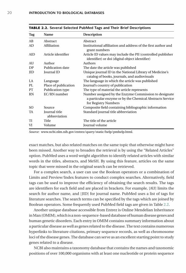
For a complex search, a user can use the Boolean operators or a combination ofLimits and Preview/Index features to conduct complex searches. Alternatively, fieldtags can be used to improve the efficiency of obtaining the search results. The tagsare identifiers for each field and are placed in brackets. For example, [AU] limits thesearch for author name, and [JID] for journal name. PubMed uses a list of tags forliterature searches. The search terms can be specified by the tags which are joined byBoolean operators. Some frequently used PubMed field tags are given in Table 2.2.
Another unique database accessible from Entrez is Online Mendelian Inheritancein Man (OMIM), which is a non-sequence-based database of human disease genes andhuman genetic disorders. Each entry in OMIM contains summary information abouta particular disease as well as genes related to the disease. The text contains numeroushyperlinks to literature citations, primary sequence records, as well as chromosomeloci of the disease genes. The database can serve as an excellent starting point to studygenes related to a disease.
NCBI also maintains a taxonomy database that contains the names and taxonomicpositions of over 100,000 organisms with at least one nucleotide or protein sequence
P1: JZP0521840988c02 CB1022/Xiong 0 521 84098 8 January 10, 2006 14:42
INFORMATION RETRIEVAL FROM BIOLOGICAL DATABASES 21
represented in the GenBank database. The taxonomy database has a hierarchical clas-sification scheme. The root level is Archaea, Eubacteria, and Eukaryota. The databaseallows the taxonomic tree for a particular organism to be displayed. The tree is basedon molecular phylogenetic data, namely, the small ribosomal RNA data.
GenBank
GenBank is the most complete collection of annotated nucleic acid sequence datafor almost every organism. The content includes genomic DNA, mRNA, cDNA, ESTs,high throughput raw sequence data, and sequence polymorphisms. There is also aGenPept database for protein sequences, the majority of which are conceptual trans-lations from DNA sequences, although a small number of the amino acid sequencesare derived using peptide sequencing techniques.
There are two ways to search for sequences in GenBank. One is using text-basedkeywords similar to a PubMed search. The other is using molecular sequences tosearch by sequence similarity using BLAST (to be described in Chapter 5).
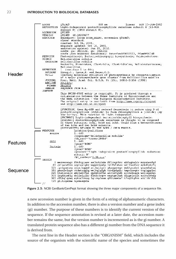
GenBank Sequence FormatTo search GenBank effectively using the text-based method requires an understandingof the GenBank sequence format. GenBank is a relational database. However, thesearch output for sequence files is produced as flat files for easy reading. The resultingflat files contain three sections – Header, Features, and Sequence entry (Fig. 2.3).There are many fields in the Header and Features sections. Each field has an uniqueidentifier for easy indexing by computer software. Understanding the structure of theGenBank files helps in designing effective search strategies.
The Header section describes the origin of the sequence, identification of the organ-ism, and unique identifiers associated with the record. The top line of the Headersection is the Locus, which contains a unique database identifier for a sequence loca-tion in the database (not a chromosome locus). The identifier is followed by sequencelength and molecule type (e.g., DNA or RNA). This is followed by a three-letter codefor GenBank divisions. There are 17 divisions in total, which were set up simply basedon convenience of data storage without necessarily having rigorous scientific basis;for example, PLN for plant, fungal, and algal sequences; PRI for primate sequences;MAM for nonprimate mammalian sequences; BCT for bacterial sequences; and ESTfor EST sequences. Next to the division is the date when the record was made public(which is different from the date when the data were submitted).
The following line, “DEFINITION,” provides the summary information for thesequence record including the name of the sequence, the name and taxonomy ofthe source organism if known, and whether the sequence is complete or partial. Thisis followed by an accession number for the sequence, which is a unique numberassigned to a piece of DNA when it was first submitted to GenBank and is perma-nently associated with that sequence. This is the number that should be cited inpublications. It has two different formats: two letters with five digits or one letter withsix digits. For a nucleotide sequence that has been translated into a protein sequence,
P1: JZP0521840988c02 CB1022/Xiong 0 521 84098 8 January 10, 2006 14:42
22 INTRODUCTION TO BIOLOGICAL DATABASES
Figure 2.3: NCBI GenBank/GenPept format showing the three major components of a sequence file.
a new accession number is given in the form of a string of alphanumeric characters.In addition to the accession number, there is also a version number and a gene index(gi) number. The purpose of these numbers is to identify the current version of thesequence. If the sequence annotation is revised at a later date, the accession num-ber remains the same, but the version number is incremented as is the gi number. Atranslated protein sequence also has a different gi number from the DNA sequence itis derived from.
The next line in the Header section is the “ORGANISM” field, which includes thesource of the organism with the scientific name of the species and sometimes the
P1: JZP0521840988c02 CB1022/Xiong 0 521 84098 8 January 10, 2006 14:42
INFORMATION RETRIEVAL FROM BIOLOGICAL DATABASES 23
tissue type. Along with the scientific name is the information of taxonomic classi-fication of the organism. Different levels of the classification are hyperlinked to theNCBI taxonomy database with more detailed descriptions. This is followed by the“REFERENCE” field, which provides the publication citation related to the sequenceentry. The REFERENCE part includes author and title information of the publishedwork (or tentative title for unpublished work). The “JOURNAL” field includes the cita-tion information as well as the date of sequence submission. The citation is oftenhyperlinked to the PubMed record for access to the original literature information.The last part of the Header is the contact information of the sequence submitter.
The “Features” section includes annotation information about the gene and geneproduct, as well as regions of biological significance reported in the sequence, withidentifiers and qualifiers. The “Source” field provides the length of the sequence,the scientific name of the organism, and the taxonomy identification number. Someoptional information includes the clone source, the tissue type and the cell line. The“gene” field is the information about the nucleotide coding sequence and its name.For DNA entries, there is a “CDS” field, which is information about the boundaries ofthe sequence that can be translated into amino acids. For eukaryotic DNA, this fieldalso contains information of the locations of exons and translated protein sequencesis entered.
The third section of the flat file is the sequence itself starting with the label“ORIGIN.” The format of the sequence display can be changed by choosing optionsat a Display pull-down menu at the upper left corner. For DNA entries, there is a BASECOUNT report that includes the numbers of A, G, C, and T in the sequence. Thissection, for both DNA or protein sequences, ends with two forward slashes (the “//”symbol).
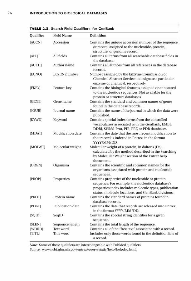
In retrieving DNA or protein sequences from GenBank, the search can be limited todifferent fields of annotation such as “organism,” “accession number,” “authors,” and“publication date.” One can use a combination of the “Limits” and “Preview/Index”options as described. Alternatively, a number of search qualifiers can be used, eachdefining one of the fields in a GenBank file. The qualifiers are similar to but not thesame as the field tags in PubMed. For example, in GenBank, [GENE] represents fieldfor gene name, [AUTH] for author name, and [ORGN] for organism name. Frequentlyused GenBank qualifiers, which have to be in uppercase and in brackets, are listed inTable 2.3.
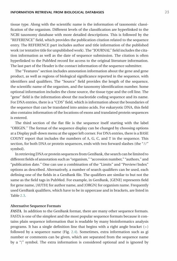
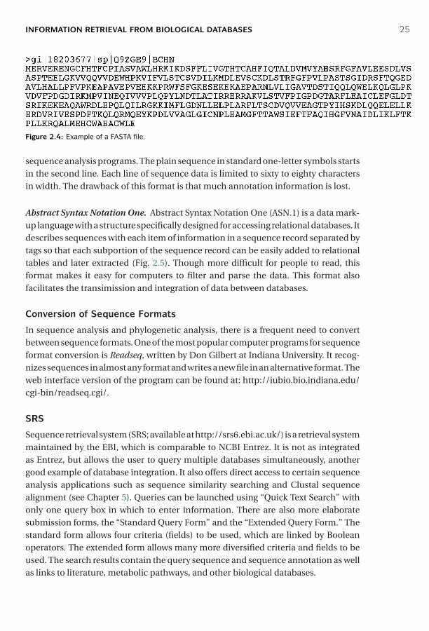
Alternative Sequence FormatsFASTA. In addition to the GenBank format, there are many other sequence formats.FASTA is one of the simplest and the most popular sequence formats because it con-tains plain sequence information that is readable by many bioinformatics analysisprograms. It has a single definition line that begins with a right angle bracket (>)followed by a sequence name (Fig. 2.4). Sometimes, extra information such as ginumber or comments can be given, which are separated from the sequence nameby a “|” symbol. The extra information is considered optional and is ignored by
P1: JZP0521840988c02 CB1022/Xiong 0 521 84098 8 January 10, 2006 14:42
24 INTRODUCTION TO BIOLOGICAL DATABASES
TABLE 2.3. Search Field Qualifiers for GenBank
Qualifier Field Name Definition
[ACCN] Accession Contains the unique accession number of the sequenceor record, assigned to the nucleotide, protein,structure, or genome record.
[ALL] All fields Contains all terms from all searchable database fields inthe database.
[AUTH] Author name Contains all authors from all references in the databaserecords.
[ECNO] EC/RN number Number assigned by the Enzyme Commission orChemical Abstract Service to designate a particularenzyme or chemical, respectively.
[FKEY] Feature key Contains the biological features assigned or annotatedto the nucleotide sequences. Not available for theprotein or structure databases.
[GENE] Gene name Contains the standard and common names of genesfound in the database records.
[JOUR] Journal name Contains the name of the journal in which the data werepublished.
[KYWD] Keyword Contains special index terms from the controlledvocabularies associated with the GenBank, EMBL,DDBJ, SWISS-Prot, PIR, PRF, or PDB databases.
[MDAT] Modification date Contains the date that the most recent modification tothat record is indexed in Entrez, in the formatYYYY/MM/DD.
[MOLWT] Molecular weight Molecular weight of a protein, in daltons (Da),calculated by the method described in the Searchingby Molecular Weight section of the Entrez helpdocument.
[ORGN] Organism Contains the scientific and common names for theorganisms associated with protein and nucleotidesequences.
[PROP] Properties Contains properties of the nucleotide or proteinsequence. For example, the nucleotide database’sproperties index includes molecule types, publicationstatus, molecule locations, and GenBank divisions.
[PROT] Protein name Contains the standard names of proteins found indatabase records.
[PDAT] Publication date Contains the date that records are released into Entrez,in the format YYYY/MM/DD.
[SQID] SeqID Contains the special string identifier for a givensequence.
[SLEN] Sequence length Contains the total length of the sequence.[WORD] Text word Contains all of the “free text” associated with a record.[TITL] Title word Includes only those words found in the definition line of
a record.
Note: Some of these qualifiers are interchangeable with PubMed qualifiers.Source: www.ncbi.nlm.nih.gov/entrez/query/static/help/helpdoc.html.
P1: JZP0521840988c02 CB1022/Xiong 0 521 84098 8 January 10, 2006 14:42
INFORMATION RETRIEVAL FROM BIOLOGICAL DATABASES 25
Figure 2.4: Example of a FASTA file.
sequence analysis programs. The plain sequence in standard one-letter symbols startsin the second line. Each line of sequence data is limited to sixty to eighty charactersin width. The drawback of this format is that much annotation information is lost.
Abstract Syntax Notation One. Abstract Syntax Notation One (ASN.1) is a data mark-up language with a structure specifically designed for accessing relational databases. Itdescribes sequences with each item of information in a sequence record separated bytags so that each subportion of the sequence record can be easily added to relationaltables and later extracted (Fig. 2.5). Though more difficult for people to read, thisformat makes it easy for computers to filter and parse the data. This format alsofacilitates the transimission and integration of data between databases.
Conversion of Sequence Formats
In sequence analysis and phylogenetic analysis, there is a frequent need to convertbetween sequence formats. One of the most popular computer programs for sequenceformat conversion is Readseq, written by Don Gilbert at Indiana University. It recog-nizes sequences in almost any format and writes a new file in an alternative format. Theweb interface version of the program can be found at: http://iubio.bio.indiana.edu/cgi-bin/readseq.cgi/.
SRS
Sequence retrieval system (SRS; available at http://srs6.ebi.ac.uk/) is a retrieval systemmaintained by the EBI, which is comparable to NCBI Entrez. It is not as integratedas Entrez, but allows the user to query multiple databases simultaneously, anothergood example of database integration. It also offers direct access to certain sequenceanalysis applications such as sequence similarity searching and Clustal sequencealignment (see Chapter 5). Queries can be launched using “Quick Text Search” withonly one query box in which to enter information. There are also more elaboratesubmission forms, the “Standard Query Form” and the “Extended Query Form.” Thestandard form allows four criteria (fields) to be used, which are linked by Booleanoperators. The extended form allows many more diversified criteria and fields to beused. The search results contain the query sequence and sequence annotation as wellas links to literature, metabolic pathways, and other biological databases.

P1: JZP0521840988c02 CB1022/Xiong 0 521 84098 8 January 10, 2006 14:42
26 INTRODUCTION TO BIOLOGICAL DATABASES
Figure 2.5: A portion of a sequence file in ASN.1 format.
P1: JZP0521840988c02 CB1022/Xiong 0 521 84098 8 January 10, 2006 14:42
FURTHER READING 27
SUMMARY
Databases are fundamental to modern biological research, especially to genomic stud-ies. The goal of a biological database is two fold: information retrieval and knowledgediscovery. Electronic databases can be constructed either as flat files, relational, orobject oriented. Flat files are simple text files and lack any form of organization tofacilitate information retrieval by computers. Relational databases organize data astables and search information among tables with shared features. Object-orienteddatabases organize data as objects and associate the objects according to hierar-chical relationships. Biological databases encompass all three types. Based on theircontent, biological databases are divided into primary, secondary, and specializeddatabases. Primary databases simply archive sequence or structure information; sec-ondary databases include further analysis on the sequences or structures. Special-ized databases cater to a particular research interest. Biological databases need to beinterconnected so that entries in one database can be cross-linked to related entriesin another database. NCBI databases accessible through Entrez are among the mostintegrated databases. Effective information retrieval involves the use of Boolean oper-ators. Entrez has additional user-friendly features to help conduct complex searches.One such option is to use Limits, Preview/Index, and History to narrow down thesearch space. Alternatively, one can use NCBI-specific field qualifiers to conductsearches. To retrieve sequence information from NCBI GenBank, an understandingof the format of GenBank sequence files is necessary. It is also important to bear inmind that sequence data in these databases are less than perfect. There are sequenceand annotation errors. Biological databases are also plagued by redundancy prob-lems. There are various solutions to correct annotation and reduce redundancy, forexample, merging redundant sequences into a single entry or store highly redundantsequences into a separate database.
FURTHER READING
Apweiler, R. 2000. Protein sequence databases. Adv. Protein Chem. 54:31–71.Blaschke, C., Hirschman, L., and Valencia, A. 2002. Information extraction in molecular biology.
Brief. Bioinform. 3:154–65.Geer, R. C., and Sayers, E. W. 2003. Entrez: Making use of its power. Brief. Bioinform. 4:179–84.Hughes, A. E. 2001. Sequence databases and the Internet. Methods Mol. Biol. 167:215–23.Patnaik, S. K., and Blumenfeld, O. O. 2001. Use of on-line tools and databases for routine
sequence analyses. Anal. Biochem. 289:1–9.Stein, L. D. 2003. Integrating biological databases. Nat. Rev. Genet. 4:337–45.

P1: JZP0521840988c02 CB1022/Xiong 0 521 84098 8 January 10, 2006 14:42
28

P1: JZP0521840988c03 CB1022/Xiong 0 521 84098 8 January 10, 2006 15:18
SECTION TWO
Sequence Alignment
29

P1: JZP0521840988c03 CB1022/Xiong 0 521 84098 8 January 10, 2006 15:18
30

P1: JZP0521840988c03 CB1022/Xiong 0 521 84098 8 January 10, 2006 15:18
CHAPTER THREE
Pairwise Sequence Alignment
Sequence comparison lies at the heart of bioinformatics analysis. It is an importantfirst step toward structural and functional analysis of newly determined sequences. Asnew biological sequences are being generated at exponential rates, sequence compari-son is becoming increasingly important to draw functional and evolutionary inferenceof a new protein with proteins already existing in the database. The most fundamentalprocess in this type of comparison is sequence alignment. This is the process by whichsequences are compared by searching for common character patterns and establish-ing residue–residue correspondence among related sequences. Pairwise sequencealignment is the process of aligning two sequences and is the basis of database sim-ilarity searching (see Chapter 4) and multiple sequence alignment (see Chapter 5).This chapter introduces the basics of pairwise alignment.
EVOLUTIONARY BASIS
DNA and proteins are products of evolution. The building blocks of these biologi-cal macromolecules, nucleotide bases, and amino acids form linear sequences thatdetermine the primary structure of the molecules. These molecules can be consid-ered molecular fossils that encode the history of millions of years of evolution. Duringthis time period, the molecular sequences undergo random changes, some of whichare selected during the process of evolution. As the selected sequences graduallyaccumulate mutations and diverge over time, traces of evolution may still remain incertain portions of the sequences to allow identification of the common ancestry. Thepresence of evolutionary traces is because some of the residues that perform key func-tional and structural roles tend to be preserved by natural selection; other residuesthat may be less crucial for structure and function tend to mutate more frequently.For example, active site residues of an enzyme family tend to be conserved becausethey are responsible for catalytic functions. Therefore, by comparing sequencesthrough alignment, patterns of conservation and variation can be identified. Thedegree of sequence conservation in the alignment reveals evolutionary relatedness ofdifferent sequences, whereas the variation between sequences reflects the changesthat have occurred during evolution in the form of substitutions, insertions, anddeletions.
Identifying the evolutionary relationships between sequences helps to characterizethe function of unknown sequences. When a sequence alignment reveals significant
31
P1: JZP0521840988c03 CB1022/Xiong 0 521 84098 8 January 10, 2006 15:18
32 PAIRWISE SEQUENCE ALIGNMENT
similarity among a group of sequences, they can be considered as belonging to thesame family (protein families will be further described in Chapter 7). If one memberwithin the family has a known structure and function, then that information can betransferred to those that have not yet been experimentally characterized. Therefore,sequence alignment can be used as basis for prediction of structure and function ofuncharacterized sequences.
Sequence alignment provides inference for the relatedness of two sequences understudy. If the two sequences share significant similarity, it is extremely unlikely thatthe extensive similarity between the two sequences has been acquired randomly,meaning that the two sequences must have derived from a common evolutionaryorigin. When a sequence alignment is generated correctly, it reflects the evolutionaryrelationship of the two sequences: regions that are aligned but not identical repre-sent residue substitutions; regions where residues from one sequence correspond tonothing in the other represent insertions or deletions that have taken place on one ofthe sequences during evolution. It is also possible that two sequences have derivedfrom a common ancestor, but may have diverged to such an extent that the com-mon ancestral relationships are not recognizable at the sequence level. In that case,the distant evolutionary relationships have to be detected using other methods (seeChapter 15).
SEQUENCE HOMOLOGY VERSUS SEQUENCE SIMILARITY
An important concept in sequence analysis is sequence homology. When twosequences are descended from a common evolutionary origin, they are said to have ahomologous relationship or share homology. A related but different term is sequencesimilarity, which is the percentage of aligned residues that are similar in physiochem-ical properties such as size, charge, and hydrophobicity.
It is important to distinguish sequence homology from the related term sequencesimilarity because the two terms are often confused by some researchers who use theminterchangeably in scientific literature. To be clear, sequence homology is an inferenceor a conclusion about a common ancestral relationship drawn from sequence simi-larity comparison when the two sequences share a high enough degree of similarity.On the other hand, similarity is a direct result of observation from the sequencealignment. Sequence similarity can be quantified using percentages; homology is aqualitative statement. For example, one may say that two sequences share 40% simi-larity. It is incorrect to say that the two sequences share 40% homology. They are eitherhomologous or nonhomologous.
Generally, if the sequence similarity level is high enough, a common evolutionaryrelationship can be inferred. In dealing with real research problems, the issue of at whatsimilarity level can one infer homologous relationships is not always clear. The answerdepends on the type of sequences being examined and sequence lengths. Nucleotidesequences consist of only four characters, and therefore, unrelated sequences have
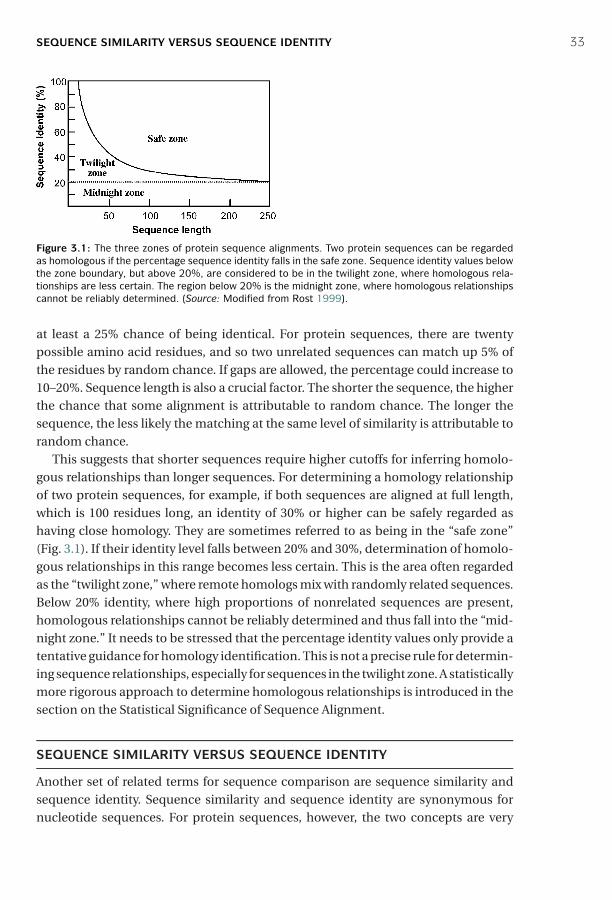
P1: JZP0521840988c03 CB1022/Xiong 0 521 84098 8 January 10, 2006 15:18
SEQUENCE SIMILARITY VERSUS SEQUENCE IDENTITY 33
Figure 3.1: The three zones of protein sequence alignments. Two protein sequences can be regardedas homologous if the percentage sequence identity falls in the safe zone. Sequence identity values belowthe zone boundary, but above 20%, are considered to be in the twilight zone, where homologous rela-tionships are less certain. The region below 20% is the midnight zone, where homologous relationshipscannot be reliably determined. (Source: Modified from Rost 1999).
at least a 25% chance of being identical. For protein sequences, there are twentypossible amino acid residues, and so two unrelated sequences can match up 5% ofthe residues by random chance. If gaps are allowed, the percentage could increase to10–20%. Sequence length is also a crucial factor. The shorter the sequence, the higherthe chance that some alignment is attributable to random chance. The longer thesequence, the less likely the matching at the same level of similarity is attributable torandom chance.
This suggests that shorter sequences require higher cutoffs for inferring homolo-gous relationships than longer sequences. For determining a homology relationshipof two protein sequences, for example, if both sequences are aligned at full length,which is 100 residues long, an identity of 30% or higher can be safely regarded ashaving close homology. They are sometimes referred to as being in the “safe zone”(Fig. 3.1). If their identity level falls between 20% and 30%, determination of homolo-gous relationships in this range becomes less certain. This is the area often regardedas the “twilight zone,” where remote homologs mix with randomly related sequences.Below 20% identity, where high proportions of nonrelated sequences are present,homologous relationships cannot be reliably determined and thus fall into the “mid-night zone.” It needs to be stressed that the percentage identity values only provide atentative guidance for homology identification. This is not a precise rule for determin-ing sequence relationships, especially for sequences in the twilight zone. A statisticallymore rigorous approach to determine homologous relationships is introduced in thesection on the Statistical Significance of Sequence Alignment.
SEQUENCE SIMILARITY VERSUS SEQUENCE IDENTITY
Another set of related terms for sequence comparison are sequence similarity andsequence identity. Sequence similarity and sequence identity are synonymous fornucleotide sequences. For protein sequences, however, the two concepts are very

P1: JZP0521840988c03 CB1022/Xiong 0 521 84098 8 January 10, 2006 15:18
34 PAIRWISE SEQUENCE ALIGNMENT
different. In a protein sequence alignment, sequence identity refers to the percent-age of matches of the same amino acid residues between two aligned sequences.Similarity refers to the percentage of aligned residues that have similar physicochem-ical characteristics and can be more readily substituted for each other.
There are two ways to calculate the sequence similarity/identity. One involves theuse of the overall sequence lengths of both sequences; the other normalizes by thesize of the shorter sequence. The first method uses the following formula:
S = [(Ls × 2)/(La + Lb)] × 100 (Eq. 3.1)
where S is the percentage sequence similarity, L s is the number of aligned residueswith similar characteristics, and L a and L b are the total lengths of each individualsequence. The sequence identity (I%) can be calculated in a similar fashion:
I = [(L i × 2)/(La + Lb)] × 100 (Eq. 3.2)
where L i is the number of aligned identical residues.The second method of calculation is to derive the percentage of identical/similar
residues over the full length of the smaller sequence using the formula:
I(S)% = L i(s)/La % (Eq. 3.3)
where L a is the length of the shorter of the two sequences.
METHODS
The overall goal of pairwise sequence alignment is to find the best pairing of twosequences, such that there is maximum correspondence among residues. To achievethis goal, one sequence needs to be shifted relative to the other to find the positionwhere maximum matches are found. There are two different alignment strategies thatare often used: global alignment and local alignment.
Global Alignment and Local Alignment
In global alignment, two sequences to be aligned are assumed to be generally simi-lar over their entire length. Alignment is carried out from beginning to end of bothsequences to find the best possible alignment across the entire length between the twosequences. This method is more applicable for aligning two closely related sequencesof roughly the same length. For divergent sequences and sequences of variablelengths, this method may not be able to generate optimal results because it failsto recognize highly similar local regions between the two sequences.
Local alignment, on the other hand, does not assume that the two sequences inquestion have similarity over the entire length. It only finds local regions with thehighest level of similarity between the two sequences and aligns these regions with-out regard for the alignment of the rest of the sequence regions. This approach can be
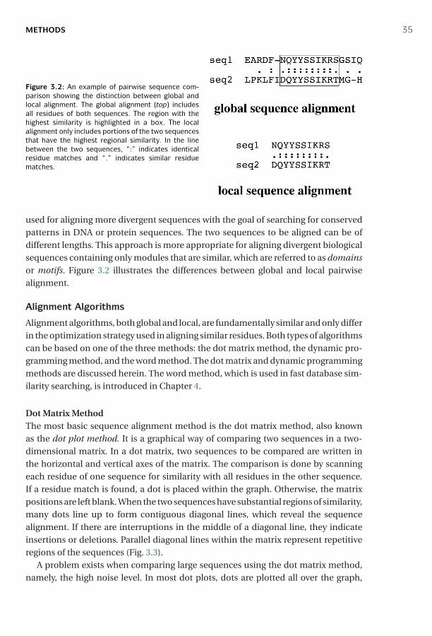
P1: JZP0521840988c03 CB1022/Xiong 0 521 84098 8 January 10, 2006 15:18
METHODS 35
Figure 3.2: An example of pairwise sequence com-parison showing the distinction between global andlocal alignment. The global alignment (top) includesall residues of both sequences. The region with thehighest similarity is highlighted in a box. The localalignment only includes portions of the two sequencesthat have the highest regional similarity. In the linebetween the two sequences, “:” indicates identicalresidue matches and “.” indicates similar residuematches.
used for aligning more divergent sequences with the goal of searching for conservedpatterns in DNA or protein sequences. The two sequences to be aligned can be ofdifferent lengths. This approach is more appropriate for aligning divergent biologicalsequences containing only modules that are similar, which are referred to as domainsor motifs. Figure 3.2 illustrates the differences between global and local pairwisealignment.
Alignment Algorithms
Alignment algorithms, both global and local, are fundamentally similar and only differin the optimization strategy used in aligning similar residues. Both types of algorithmscan be based on one of the three methods: the dot matrix method, the dynamic pro-gramming method, and the word method. The dot matrix and dynamic programmingmethods are discussed herein. The word method, which is used in fast database sim-ilarity searching, is introduced in Chapter 4.
Dot Matrix MethodThe most basic sequence alignment method is the dot matrix method, also knownas the dot plot method. It is a graphical way of comparing two sequences in a two-dimensional matrix. In a dot matrix, two sequences to be compared are written inthe horizontal and vertical axes of the matrix. The comparison is done by scanningeach residue of one sequence for similarity with all residues in the other sequence.If a residue match is found, a dot is placed within the graph. Otherwise, the matrixpositions are left blank. When the two sequences have substantial regions of similarity,many dots line up to form contiguous diagonal lines, which reveal the sequencealignment. If there are interruptions in the middle of a diagonal line, they indicateinsertions or deletions. Parallel diagonal lines within the matrix represent repetitiveregions of the sequences (Fig. 3.3).
A problem exists when comparing large sequences using the dot matrix method,namely, the high noise level. In most dot plots, dots are plotted all over the graph,
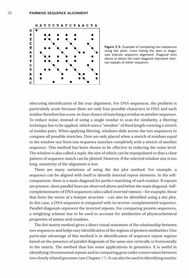
P1: JZP0521840988c03 CB1022/Xiong 0 521 84098 8 January 10, 2006 15:18
36 PAIRWISE SEQUENCE ALIGNMENT
Figure 3.3: Example of comparing two sequencesusing dot plots. Lines linking the dots in diago-nals indicate sequence alignment. Diagonal linesabove or below the main diagonal represent inter-nal repeats of either sequence.
obscuring identification of the true alignment. For DNA sequences, the problem isparticularly acute because there are only four possible characters in DNA and eachresidue therefore has a one-in-four chance of matching a residue in another sequence.To reduce noise, instead of using a single residue to scan for similarity, a filteringtechnique has to be applied, which uses a “window” of fixed length covering a stretchof residue pairs. When applying filtering, windows slide across the two sequences tocompare all possible stretches. Dots are only placed when a stretch of residues equalto the window size from one sequence matches completely with a stretch of anothersequence. This method has been shown to be effective in reducing the noise level.The window is also called a tuple, the size of which can be manipulated so that a clearpattern of sequence match can be plotted. However, if the selected window size is toolong, sensitivity of the alignment is lost.
There are many variations of using the dot plot method. For example, asequence can be aligned with itself to identify internal repeat elements. In the self-comparison, there is a main diagonal for perfect matching of each residue. If repeatsare present, short parallel lines are observed above and below the main diagonal. Self-complementarity of DNA sequences (also called inverted repeats) – for example, thosethat form the stems of a hairpin structure – can also be identified using a dot plot.In this case, a DNA sequence is compared with its reverse-complemented sequence.Parallel diagonals represent the inverted repeats. For comparing protein sequences,a weighting scheme has to be used to account for similarities of physicochemicalproperties of amino acid residues.
The dot matrix method gives a direct visual statement of the relationship betweentwo sequences and helps easy identification of the regions of greatest similarities. Oneparticular advantage of this method is in identification of sequence repeat regionsbased on the presence of parallel diagonals of the same size vertically or horizontallyin the matrix. The method thus has some applications in genomics. It is useful inidentifying chromosomal repeats and in comparing gene order conservation betweentwo closely related genomes (see Chapter 17). It can also be used in identifying nucleic
P1: JZP0521840988c03 CB1022/Xiong 0 521 84098 8 January 10, 2006 15:18
METHODS 37
acid secondary structures through detecting self-complementarity of a sequence (seeChapter 16).
The dot matrix method displays all possible sequence matches. However, it is oftenup to the user to construct a full alignment with insertions and deletions by linkingnearby diagonals. Another limitation of this visual analysis method is that it lacksstatistical rigor in assessing the quality of the alignment. The method is also restrictedto pairwise alignment. It is difficult for the method to scale up to multiple alignment.The following are examples of web servers that provide pairwise sequence comparisonusing dot plots.
Dotmatcher (bioweb.pasteur.fr/seqanal/interfaces/dotmatcher.html) and Dottup(bioweb.pasteur.fr/seqanal/interfaces/dottup.html) are two programs of the EMBOSSpackage, which have been made available online. Dotmatcher aligns and displays dotplots of two input sequences (DNA or proteins) in FASTA format. A window of specifiedlength and a scoring scheme are used. Diagonal lines are only plotted over the positionof the windows if the similarity is above a certain threshold. Dottup aligns sequencesusing the word method (to be described in Chapter 4) and is capable of handlinggenome-length sequences. Diagonal lines are only drawn if exact matches of wordsof specified length are found.
Dothelix (www.genebee.msu.su/services/dhm/advanced.html) is a dot matrixprogram for DNA or protein sequences. The program has a number of options forlength threshold (similar to window size) and implements scoring matrices for pro-tein sequences. In addition to drawing diagonal lines with similarity scores above acertain threshold, the program displays actual pairwise alignment.
MatrixPlot (www.cbs.dtu.dk/services/MatrixPlot/) is a more sophisticated matrixplot program for alignment of protein and nucleic acid sequences. The user has theoption of adding information such as sequence logo profiles (see Chapter 7) anddistance matrices from known three-dimensional structures of proteins or nucleicacids. Instead of using dots and lines, the program uses colored grids to indicatealignment or other user-defined information.
Dynamic Programming MethodDynamic programming is a method that determines optimal alignment by match-ing two sequences for all possible pairs of characters between the two sequences.It is fundamentally similar to the dot matrix method in that it also creates a two-dimensional alignment grid. However, it finds alignment in a more quantitative way byconverting a dot matrix into a scoring matrix to account for matches and mismatchesbetween sequences. By searching for the set of highest scores in this matrix, the bestalignment can be accurately obtained.
Dynamic programming works by first constructing a two-dimensional matrixwhose axes are the two sequences to be compared. The residue matching is accordingto a particular scoring matrix. The scores are calculated one row at a time. This startswith the first row of one sequence, which is used to scan through the entire lengthof the other sequence, followed by scanning of the second row. The matching scores
P1: JZP0521840988c03 CB1022/Xiong 0 521 84098 8 January 10, 2006 15:18
38 PAIRWISE SEQUENCE ALIGNMENT
are calculated. The scanning of the second row takes into account the scores alreadyobtained in the first round. The best score is put into the bottom right corner of anintermediate matrix (Fig. 3.4). This process is iterated until values for all the cells arefilled. Thus, the scores are accumulated along the diagonal going from the upper leftcorner to the lower right corner. Once the scores have been accumulated in matrix,the next step is to find the path that represents the optimal alignment. This is doneby tracing back through the matrix in reverse order from the lower right-hand cornerof the matrix toward the origin of the matrix in the upper left-hand corner. The bestmatching path is the one that has the maximum total score (see Fig. 3.4). If two ormore paths reach the same highest score, one is chosen arbitrarily to represent thebest alignment. The path can also move horizontally or vertically at a certain point,which corresponds to introduction of a gap or an insertion or deletion for one of thetwo sequences.
Gap Penalties. Performing optimal alignment between sequences often involvesapplying gaps that represent insertions and deletions. Because in natural evolu-tionary processes insertion and deletions are relatively rare in comparison to sub-stitutions, introducing gaps should be made more difficult computationally, reflect-ing the rarity of insertional and deletional events in evolution. However, assigningpenalty values can be more or less arbitrary because there is no evolutionary theoryto determine a precise cost for introducing insertions and deletions. If the penaltyvalues are set too low, gaps can become too numerous to allow even nonrelatedsequences to be matched up with high similarity scores. If the penalty values areset too high, gaps may become too difficult to appear, and reasonable alignmentcannot be achieved, which is also unrealistic. Through empirical studies for globularproteins, a set of penalty values have been developed that appear to suit most align-ment purposes. They are normally implemented as default values in most alignmentprograms.
Another factor to consider is the cost difference between opening a gap and extend-ing an existing gap. It is known that it is easier to extend a gap that has already beenstarted. Thus, gap opening should have a much higher penalty than gap extension.This is based on the rationale that if insertions and deletions ever occur, several adja-cent residues are likely to have been inserted or deleted together. These differentialgap penalties are also referred to as affine gap penalties. The normal strategy is to usepreset gap penalty values for introducing and extending gaps. For example, one mayuse a −12/ − 1 scheme in which the gap opening penalty is −12 and the gap exten-sion penalty −1. The total gap penalty (W ) is a linear function of gap length, which iscalculated using the formula:
W = γ + δ × (k − 1) (Eq. 3.4)
where γ is the gap opening penalty, δ is the gap extension penalty, and k is the lengthof the gap. Besides the affine gap penalty, a constant gap penalty is sometimes alsoused, which assigns the same score for each gap position regardless whether it is
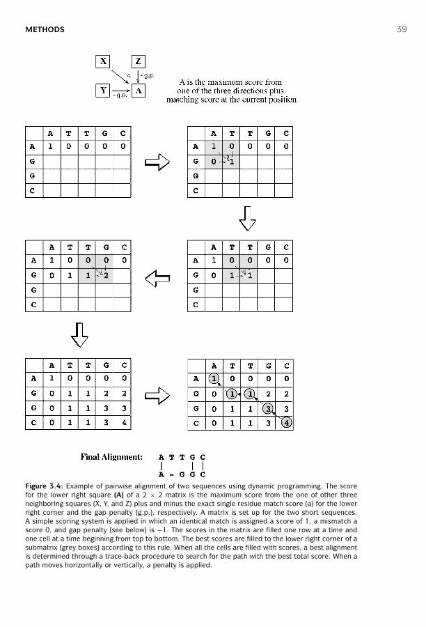
P1: JZP0521840988c03 CB1022/Xiong 0 521 84098 8 January 10, 2006 15:18
METHODS 39
Figure 3.4: Example of pairwise alignment of two sequences using dynamic programming. The scorefor the lower right square (A) of a 2 × 2 matrix is the maximum score from the one of other threeneighboring squares (X, Y, and Z) plus and minus the exact single residue match score (a) for the lowerright corner and the gap penalty (g.p.), respectively. A matrix is set up for the two short sequences.A simple scoring system is applied in which an identical match is assigned a score of 1, a mismatch ascore 0, and gap penalty (see below) is −1. The scores in the matrix are filled one row at a time andone cell at a time beginning from top to bottom. The best scores are filled to the lower right corner of asubmatrix (grey boxes) according to this rule. When all the cells are filled with scores, a best alignmentis determined through a trace-back procedure to search for the path with the best total score. When apath moves horizontally or vertically, a penalty is applied.
P1: JZP0521840988c03 CB1022/Xiong 0 521 84098 8 January 10, 2006 15:18
40 PAIRWISE SEQUENCE ALIGNMENT
opening or extending. However, this penalty scheme has been found to be less realisticthan the affine penalty.
Gaps at the terminal regions are often treated with no penalty because in realitymany true homologous sequences are of different lengths. Consequently, end gapscan be allowed to be free to avoid getting unrealistic alignments.
Dynamic Programming for Global Alignment. The classical global pairwise align-ment algorithm using dynamic programming is the Needleman–Wunsch algorithm.In this algorithm, an optimal alignment is obtained over the entire lengths of thetwo sequences. It must extend from the beginning to the end of both sequences toachieve the highest total score. In other words, the alignment path has to go from thebottom right corner of the matrix to the top left corner. The drawback of focusing ongetting a maximum score for the full-length sequence alignment is the risk of missingthe best local similarity. This strategy is only suitable for aligning two closely relatedsequences that are of the same length. For divergent sequences or sequences withdifferent domain structures, the approach does not produce optimal alignment. Oneof the few web servers dedicated to global pairwise alignment is GAP.
GAP (http://bioinformatics.iastate.edu/aat/align/align.html) is a web-based pair-wise global alignment program. It aligns two sequences without penalizing terminalgaps so similar sequences of unequal lengths can be aligned. To be able to insert longgaps in the alignment, such gaps are treated with a constant penalty. This feature isuseful in aligning cDNA to exons in genomic DNA containing the same gene.
Dynamic Programming for Local Alignment. In regular sequence alignment, thedivergence level between the two sequences to be aligned is not easily known. Thesequence lengths of the two sequences may also be unequal. In such cases, identi-fication of regional sequence similarity may be of greater significance than findinga match that includes all residues. The first application of dynamic programming inlocal alignment is the Smith–Waterman algorithm. In this algorithm, positive scoresare assigned for matching residues and zeros for mismatches. No negative scores areused. A similar tracing-back procedure is used in dynamic programming. However,the alignment path may begin and end internally along the main diagonal. It startswith the highest scoring position and proceeds diagonally up to the left until reachinga cell with a zero. Gaps are inserted if necessary. In this case, affine gap penalty is oftenused. Occasionally, several optimally aligned segments with best scores are obtained.As in the global alignment, the final result is influenced by the choice of scoring sys-tems (to be described next) used. The goal of local alignment is to get the highestalignment score locally, which may be at the expense of the highest possible overallscore for a full-length alignment. This approach may be suitable for aligning divergentsequences or sequences with multiple domains that may be of different origins. Mostcommonly used pairwise alignment web servers apply the local alignment strategy,which include SIM, SSEARCH, and LALIGN.
P1: JZP0521840988c03 CB1022/Xiong 0 521 84098 8 January 10, 2006 15:18
SCORING MATRICES 41
SIM (http://bioinformatics.iastate.edu/aat/align/align.html) is a web-based pro-gram for pairwise alignment using the Smith–Waterman algorithm that finds the bestscored nonoverlapping local alignments between two sequences. It is able to han-dle tens of kilobases of genomic sequence. The user has the option to set a scoringmatrix and gap penalty scores. A specified number of best scored alignments areproduced.
SSEARCH (http://pir.georgetown.edu/pirwww/search/pairwise.html) is a simpleweb-based programs that uses the Smith–Waterman algorithm for pairwise alignmentof sequences. Only one best scored alignment is given. There is no option for scoringmatrices or gap penalty scores.
LALIGN (www.ch.embnet.org/software/LALIGN form.html) is a web-based pro-gram that uses a variant of the Smith–Waterman algorithm to align two sequences.Unlike SSEARCH, which returns the single best scored alignment, LALIGN gives aspecified number of best scored alignments. The user has the option to set the scor-ing matrix and gap penalty scores. The same web interface also provides an optionfor global alignment performed by the ALIGN program.
SCORING MATRICES
In the dynamic programming algorithm presented, the alignment procedure has tomake use of a scoring system, which is a set of values for quantifying the likelihood ofone residue being substituted by another in an alignment. The scoring systems is calleda substitution matrix and is derived from statistical analysis of residue substitutiondata from sets of reliable alignments of highly related sequences.
Scoring matrices for nucleotide sequences are relatively simple. A positive valueor high score is given for a match and a negative value or low score for a mismatch.This assignment is based on the assumption that the frequencies of mutation areequal for all bases. However, this assumption may not be realistic; observations showthat transitions (substitutions between purines and purines or between pyrimidinesand pyrimidines) occur more frequently than transversions (substitutions betweenpurines and pyrimidines). Therefore, a more sophisticated statistical model with dif-ferent probability values to reflect the two types of mutations is needed (see the Kimuramodel in Chapter 10).
Scoring matrices for amino acids are more complicated because scoring has toreflect the physicochemical properties of amino acid residues, as well as the likelihoodof certain residues being substituted among true homologous sequences. Certainamino acids with similar physicochemical properties can be more easily substitutedthan those without similar characteristics. Substitutions among similar residues arelikely to preserve the essential functional and structural features. However, substi-tutions between residues of different physicochemical properties are more likely tocause disruptions to the structure and function. This type of disruptive substitutionis less likely to be selected in evolution because it renders nonfunctional proteins.

P1: JZP0521840988c03 CB1022/Xiong 0 521 84098 8 January 10, 2006 15:18
42 PAIRWISE SEQUENCE ALIGNMENT
For example, phenylalanine, tyrosine, and tryptophan all share aromatic ring struc-tures. Because of their chemical similarities, they are easily substituted for each otherwithout perturbing the regular function and structure of the protein. Similarly, argi-nine, lysine, and histidine are all large basic residues and there is a high probabilityof them being substituted for each other. Aspartic acid, glutamic acid, asparagine,and glutamine belong to the acid and acid amide groups and can be associated withrelatively high frequencies of substitution. The hydrophobic residue group includesmethionine, isoleucine, leucine, and valine. Small and polar residues include serine,threonine, and cysteine. Residues within these groups have high likelihoods of beingsubstituted for each other. However, cysteine contains a sulfhydryl group that playsa role in metal binding, active site, and disulfide bond formation. Substitution ofcysteine with other residues therefore often abolishes the enzymatic activity or desta-bilizes the protein structure. It is thus a very infrequently substituted residue. Thesmall and nonpolar residues such as glycine and proline are also unique in that theirpresence often disrupts regular protein secondary structures (see Chapter 12). Thus,substitutions with these residues do not frequently occur. For more information ongrouping amino acids based on physicochemical properties, see Table 12.1.
Amino Acid Scoring Matrices
Amino acid substitution matrices, which are 20 × 20 matrices, have been devised toreflect the likelihood of residue substitutions. There are essentially two types of aminoacid substitution matrices. One type is based on interchangeability of the geneticcode or amino acid properties, and the other is derived from empirical studies ofamino acid substitutions. Although the two different approaches coincide to a certainextent, the first approach, which is based on the genetic code or the physicochemicalfeatures of amino acids, has been shown to be less accurate than the second approach,which is based on surveys of actual amino acid substitutions among related proteins.Thus, the empirical approach has gained the most popularity in sequence alignmentapplications and is the focus of our next discussion.
The empirical matrices, which include PAM and BLOSUM matrices, are derivedfrom actual alignments of highly similar sequences. By analyzing the probabilitiesof amino acid substitutions in these alignments, a scoring system can be devel-oped by giving a high score for a more likely substitution and a low score for a raresubstitution.
For a given substitution matrix, a positive score means that the frequency of aminoacid substitutions found in a data set of homologous sequences is greater than wouldhave occurred by random chance. They represent substitutions of very similar residuesor identical residues. A zero score means that the frequency of amino acid substitutionsfound in the homologous sequence data set is equal to that expected by chance. Inthis case, the relationship between the amino acids is weakly similar at best in termsof physicochemical properties. A negative score means that the frequency of aminoacid substitutions found in the homologous sequence data set is less than would
P1: JZP0521840988c03 CB1022/Xiong 0 521 84098 8 January 10, 2006 15:18
SCORING MATRICES 43
have occurred by random chance. This normally occurs with substitutions betweendissimilar residues.
The substitution matrices apply logarithmic conversions to describe the probabil-ity of amino acid substitutions. The converted values are the so-called log-odds scores(or log-odds ratios), which are logarithmic ratios of the observed mutation frequencydivided by the probability of substitution expected by random chance. The conversioncan be either to the base of 10 or to the base of 2. For example, in an alignment thatinvolves ten sequences, each having only one aligned position, nine of the sequencesare F (phenylalanine) and the remaining one I (isoleucine). The observed frequencyof I being substituted by F is one in ten (0.1), whereas the probability of I being sub-stituted by F by random chance is one in twenty (0.05). Thus, the ratio of the twoprobabilities is 2 (0.1/0.05). After taking this ratio to the logarithm to the base of 2, thismakes the log odds equal to 1. This value can then be interpreted as the likelihood ofsubstitution between the two residues being 2 1, which is two times more frequentlythan by random chance.
PAM MatricesThe PAM matrices (also called Dayhoff PAM matrices) were first constructed byMargaret Dayhoff, who compiled alignments of seventy-one groups of very closelyrelated protein sequences. PAM stands for “point accepted mutation” (although“accepted point mutation” or APM may be a more appropriate term, PAM is easier topronounce). Because of the use of very closely related homologs, the observed muta-tions were not expected to significantly change the common function of the proteins.Thus, the observed amino acid mutations are considered to be accepted by naturalselection.
These protein sequences were clustered based on phylogenetic reconstructionusing maximum parsimony (see Chapter 11). The PAM matrices were subsequentlyderived based on the evolutionary divergence between sequences of the same cluster.One PAM unit is defined as 1% of the amino acid positions that have been changed.To construct a PAM1 substitution table, a group of closely related sequences withmutation frequencies corresponding to one PAM unit is chosen. Based on the col-lected mutational data from this group of sequences, a substitution matrix can bederived.
Construction of the PAM1 matrix involves alignment of full-length sequences andsubsequent construction of phylogenetic trees using the parsimony principle. Thisallows computation of ancestral sequences for each internal node of the trees (seeChapter 11). Ancestral sequence information is used to count the number of sub-stitutions along each branch of a tree. The PAM score for a particular residue pairis derived from a multistep procedure involving calculations of relative mutability(which is the number of mutational changes from a common ancestor for a particularamino acid residue divided by the total number of such residues occurring in analignment), normalization of the expected residue substitution frequencies by ran-dom chance, and logarithmic transformation to the base of 10 of the normalized
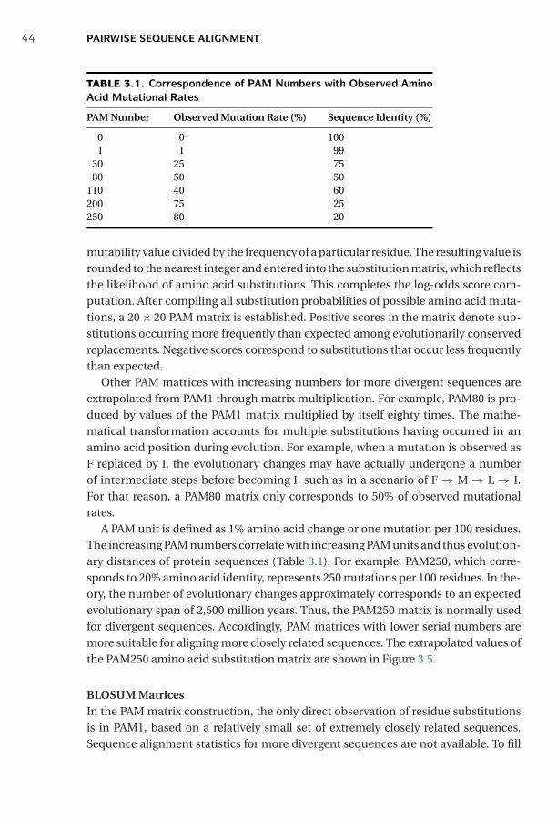
P1: JZP0521840988c03 CB1022/Xiong 0 521 84098 8 January 10, 2006 15:18
44 PAIRWISE SEQUENCE ALIGNMENT
TABLE 3.1. Correspondence of PAM Numbers with Observed AminoAcid Mutational Rates
PAM Number Observed Mutation Rate (%) Sequence Identity (%)
0 0 1001 1 99
30 25 7580 50 50
110 40 60200 75 25250 80 20
mutability value divided by the frequency of a particular residue. The resulting value isrounded to the nearest integer and entered into the substitution matrix, which reflectsthe likelihood of amino acid substitutions. This completes the log-odds score com-putation. After compiling all substitution probabilities of possible amino acid muta-tions, a 20 × 20 PAM matrix is established. Positive scores in the matrix denote sub-stitutions occurring more frequently than expected among evolutionarily conservedreplacements. Negative scores correspond to substitutions that occur less frequentlythan expected.
Other PAM matrices with increasing numbers for more divergent sequences areextrapolated from PAM1 through matrix multiplication. For example, PAM80 is pro-duced by values of the PAM1 matrix multiplied by itself eighty times. The mathe-matical transformation accounts for multiple substitutions having occurred in anamino acid position during evolution. For example, when a mutation is observed asF replaced by I, the evolutionary changes may have actually undergone a numberof intermediate steps before becoming I, such as in a scenario of F → M → L → I.For that reason, a PAM80 matrix only corresponds to 50% of observed mutationalrates.
A PAM unit is defined as 1% amino acid change or one mutation per 100 residues.The increasing PAM numbers correlate with increasing PAM units and thus evolution-ary distances of protein sequences (Table 3.1). For example, PAM250, which corre-sponds to 20% amino acid identity, represents 250 mutations per 100 residues. In the-ory, the number of evolutionary changes approximately corresponds to an expectedevolutionary span of 2,500 million years. Thus, the PAM250 matrix is normally usedfor divergent sequences. Accordingly, PAM matrices with lower serial numbers aremore suitable for aligning more closely related sequences. The extrapolated values ofthe PAM250 amino acid substitution matrix are shown in Figure 3.5.
BLOSUM MatricesIn the PAM matrix construction, the only direct observation of residue substitutionsis in PAM1, based on a relatively small set of extremely closely related sequences.Sequence alignment statistics for more divergent sequences are not available. To fill

P1: JZP0521840988c03 CB1022/Xiong 0 521 84098 8 January 10, 2006 15:18
SCORING MATRICES 45
Figure 3.5: PAM250 amino acid substitution matrix. Residues are grouped according to physicochem-ical similarities.
in the gap, a new set of substitution matrices have been developed. This is theseries of blocks amino acid substitution matrices (BLOSUM), all of which are derivedbased on direct observation for every possible amino acid substitution in multiplesequence alignments. These were constructed based on more than 2,000 conservedamino acid patterns representing 500 groups of protein sequences. The sequencepatterns, also called blocks, are ungapped alignments of less than sixty amino acidresidues in length. The frequencies of amino acid substitutions of the residues inthese blocks are calculated to produce a numerical table, or block substitutionmatrix.
Instead of using the extrapolation function, the BLOSUM matrices are actual per-centage identity values of sequences selected for construction of the matrices. Forexample, BLOSUM62 indicates that the sequences selected for constructing the matrixshare an average identity value of 62%. Other BLOSUM matrices based on sequencegroups of various identity levels have also been constructed. In the reversing orderas the PAM numbering system, the lower the BLOSUM number, the more divergentsequences they represent.
The BLOSUM score for a particular residue pair is derived from the log ratio ofobserved residue substitution frequency versus the expected probability of a particu-lar residue. The log odds is taken to the base of 2 instead of 10 as in the PAM matrices.The resulting value is rounded to the nearest integer and entered into the substi-tution matrix. As in the PAM matrices, positive and negative values correspond tosubstitutions that occur more or less frequently than expected among evolutionarily
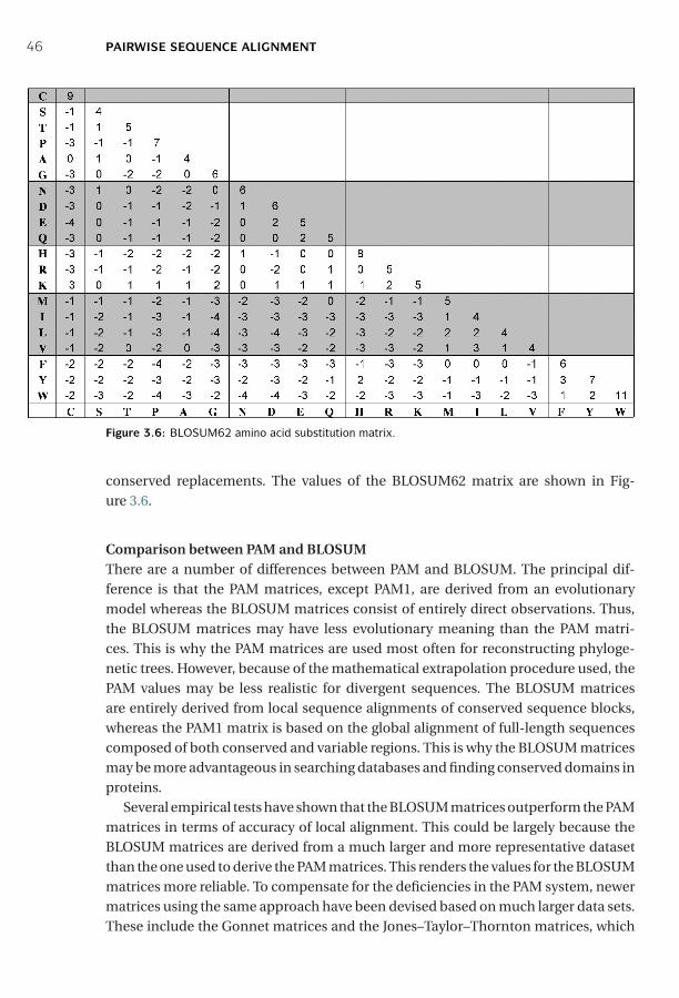
P1: JZP0521840988c03 CB1022/Xiong 0 521 84098 8 January 10, 2006 15:18
46 PAIRWISE SEQUENCE ALIGNMENT
Figure 3.6: BLOSUM62 amino acid substitution matrix.
conserved replacements. The values of the BLOSUM62 matrix are shown in Fig-ure 3.6.
Comparison between PAM and BLOSUMThere are a number of differences between PAM and BLOSUM. The principal dif-ference is that the PAM matrices, except PAM1, are derived from an evolutionarymodel whereas the BLOSUM matrices consist of entirely direct observations. Thus,the BLOSUM matrices may have less evolutionary meaning than the PAM matri-ces. This is why the PAM matrices are used most often for reconstructing phyloge-netic trees. However, because of the mathematical extrapolation procedure used, thePAM values may be less realistic for divergent sequences. The BLOSUM matricesare entirely derived from local sequence alignments of conserved sequence blocks,whereas the PAM1 matrix is based on the global alignment of full-length sequencescomposed of both conserved and variable regions. This is why the BLOSUM matricesmay be more advantageous in searching databases and finding conserved domains inproteins.
Several empirical tests have shown that the BLOSUM matrices outperform the PAMmatrices in terms of accuracy of local alignment. This could be largely because theBLOSUM matrices are derived from a much larger and more representative datasetthan the one used to derive the PAM matrices. This renders the values for the BLOSUMmatrices more reliable. To compensate for the deficiencies in the PAM system, newermatrices using the same approach have been devised based on much larger data sets.These include the Gonnet matrices and the Jones–Taylor–Thornton matrices, which

P1: JZP0521840988c03 CB1022/Xiong 0 521 84098 8 January 10, 2006 15:18
STATISTICAL SIGNIFICANCE OF SEQUENCE ALIGNMENT 47
Figure 3.7: Gumble extreme value distribution for alignment scores. The distribution can be expressedas P = 1− e − Kmne-λx, where m and n are the sequence lengths, λ is a scaling factor for the scoringmatrix used, and K is a constant that depends on the scoring matrix and gap penalty combination thatis used. The x-axis of the curve indicates the standard deviation of the distribution; the y-axis indicatesthe alignment scores in arbitrary units.
have been shown to have equivalent performance to BLOSUM in regular alignment,but are particularly robust in phylogenetic tree construction.
STATISTICAL SIGNIFICANCE OF SEQUENCE ALIGNMENT
When given a sequence alignment showing a certain degree of similarity, it is oftenimportant to ask whether the observed sequence alignment can occur by randomchance or the alignment is indeed statistically sound. The truly statistically signifi-cant sequence alignment will be able to provide evidence of homology between thesequences involved.
Solving this problem requires a statistical test of the alignment scores of two unre-lated sequences of the same length. By calculating alignment scores of a large numberof unrelated sequence pairs, a distribution model of the randomized sequence scorescan be derived. From the distribution, a statistical test can be performed based on thenumber of standard deviations from the average score. Many studies have demon-strated that the distribution of similarity scores assumes a peculiar shape that resem-bles a highly skewed normal distribution with a long tail on one side (Fig. 3.7). Thedistribution matches the “Gumble extreme value distribution” for which a mathemati-cal expression is available. This means that, given a sequence similarity value, by usingthe mathematical formula for the extreme distribution, the statistical significance canbe accurately estimated.
The statistical test for the relatedness of two sequences can be performed usingthe following procedure. An optimal alignment between two given sequences is firstobtained. Unrelated sequences of the same length are then generated through a ran-domization process in which one of the two sequences is randomly shuffled. A new
P1: JZP0521840988c03 CB1022/Xiong 0 521 84098 8 January 10, 2006 15:18
48 PAIRWISE SEQUENCE ALIGNMENT
alignment score is then computed for the shuffled sequence pair. More such scoresare similarly obtained through repeated shuffling. The pool of alignment scores fromthe shuffled sequences is used to generate parameters for the extreme distribution.The original alignment score is then compared against the distribution of randomalignments to determine whether the score is beyond random chance. If the scoreis located in the extreme margin of the distribution, that means that the alignmentbetween the two sequences is unlikely due to random chance and is thus consideredsignificant. A P-value is given to indicate the probability that the original alignmentis due to random chance.
A P-value resulting from the test provides a much more reliable indicator of pos-sible homologous relationships than using percent identity values. It is thus impor-tant to know how to interpret the P-values. It has been shown that if a P-value issmaller than 10−100, it indicates an exact match between the two sequences. If theP-value is in the range of 10−50 to 10−100, it is considered to be a nearly identicalmatch. A P-value in the range of 10−5 to 10−50 is interpreted as sequences having clearhomology. A P-value in the range of 10−1 to 10−5 indicates possible distant homologs.If P is larger than 10−1, the two sequence may be randomly related. However, thecaveat is that sometimes truly related protein sequences may lack the statistical sig-nificance at the sequence level owing to fast divergence rates. Their evolutionary rela-tionships can nonetheless be revealed at the three-dimensional structural level (seeChapter 15).
These statistics were derived from ungapped local sequence alignments. It is notknown whether the Gumble distribution applies equally well to gapped alignments.However, for all practical purposes, it is reasonable to assume that scores for gappedalignments essentially fit the same distribution. A frequently used software programfor assessing statistical significance of a pairwise alignment is the PRSS program.
PRSS (Probability of Random Shuffles; www.ch.embnet.org/software/PRSS form.html) is a web-based program that can be used to evaluate the statistical signifi-cance of DNA or protein sequence alignment. It first aligns two sequences using theSmith–Waterman algorithm and calculates the score. It then holds one sequence in itsoriginal form and randomizes the order of residues in the other sequence. The shuffledsequence is realigned with the unshuffled sequence. The resulting alignment score isrecorded. This process is iterated many (normally 1,000) times to help generate datafor fitting the Gumble distribution. The original alignment score is then comparedagainst the overall score distribution to derive a P-value. The major feature of theprogram is that it allows partial shuffling. For example, shuffling can be restricted toresidues within a local window of 25–40, whereas the residues outside the windowremain unchanged.
SUMMARY
Pairwise sequence alignment is the fundamental component of many bioinformaticsapplications. It is extremely useful in structural, functional, and evolutionary analyses
P1: JZP0521840988c03 CB1022/Xiong 0 521 84098 8 January 10, 2006 15:18
FURTHER READING 49
of sequences. Pairwise sequence alignment provides inference for the relatedness oftwo sequences. Strongly similar sequences are often homologous. However, a dis-tinction needs to be made between sequence homology and similarity. The formeris inference drawn from sequence comparison, whereas the latter relates to actualobservation after sequence alignment. For protein sequences, identity values frompairwise alignment are often used to infer homology, although this approach can berather imprecise.
There are two sequence alignment strategies, local alignment and global align-ment, and three types of algorithm that perform both local and global alignments.They are the dot matrix method, dynamic programming method, and word method.The dot matrix method is useful in visually identifying similar regions, but lacks thesophistication of the other two methods. Dynamic programming is an exhaustive andquantitative method to find optimal alignments. This method effectively works inthree steps. It first produces a sequence versus sequence matrix. The second step isto accumulate scores in the matrix. The last step is to trace back through the matrix inreverse order to identify the highest scoring path. This scoring step involves the useof scoring matrices and gap penalties.
Scoring matrices describe the statistical probabilities of one residue being sub-stituted by another. PAM and BLOSUM are the two most commonly used matricesfor aligning protein sequences. The PAM matrices involve the use of evolutionarymodels and extrapolation of probability values from alignment of close homologs tomore divergent ones. In contrast, the BLOSUM matrices are derived from actual align-ment. The PAM and BLOSUM serial numbers also have opposite meanings. Matricesof high PAM numbers are used to align divergent sequences and low PAM numbersfor aligning closely related sequences. In practice, if one is uncertain about whichmatrix to use, it is advisable to test several matrices and choose the one that gives thebest alignment result. Statistical significance of pairwise sequence similarity can betested using a randomization test where score distribution follows an extreme valuedistribution.
FURTHER READING
Batzoglou, S. 2005. The many faces of sequence alignment. Brief. Bioinformatics 6:6–22.Brenner, S. E., Chothia, C., and Hubbard, T. J. 1998. Assessing sequence comparison methods
with reliable structurally identified distant evolutionary relationships. Proc. Natl. Acad. Sci. US A 95:6073–8.
Chao, K.-M., Pearson, W. R., and Miller, W. 1992. Aligning two sequences within a specifieddiagonal band. Comput. Appl. Biosci. 8:481–7.
Henikoff, S., and Henikoff, J. G. 1992. Amino acid substitution matrices from protein blocks.Proc. Natl. Acad. Sci. U S A 89:10915–19.
Huang, X. 1994. On global sequence alignment. Comput. Appl. Biosci. 10:227–35.Pagni, M., and Jongeneel, V. 2001. Making sense of score statistics for sequence alignments.
Brief. Bioinformatics 2:51–67.Pearson, W. R. 1996. Effective protein sequence comparison. Methods Enzymol. 266:227–58.

P1: JZP0521840988c03 CB1022/Xiong 0 521 84098 8 January 10, 2006 15:18
50 PAIRWISE SEQUENCE ALIGNMENT
Rost, B. 1999. Twilight zone of protein sequence alignments. Protein Eng. 12:85–94.States, D. J., Gish, W., and Altschul, S. F. 1991. Improved sensitivity of nucleic acid database
searches using application-specific scoring matrices. Methods 3:66–70.Valdar, W. S. 2002. Scoring residue conservation. Proteins. 48:227–41.Vingron, M., and Waterman, M. S. 1994. Sequence alignment and penalty scores. J. Mol. Biol.
235:1–12.
P1: JZP0521840988c04 CB1022/Xiong 0 521 84098 8 January 10, 2006 15:4
CHAPTER FOUR
Database Similarity Searching
A main application of pairwise alignment is retrieving biological sequences indatabases based on similarity. This process involves submission of a query sequenceand performing a pairwise comparison of the query sequence with all individualsequences in a database. Thus, database similarity searching is pairwise alignmenton a large scale. This type of searching is one of the most effective ways to assign puta-tive functions to newly determined sequences. However, the dynamic programmingmethod described in Chapter 3 is slow and impractical to use in most cases. Specialsearch methods are needed to speed up the computational process of sequence com-parison. The theory and applications of the database searching methods are discussedin this chapter.
UNIQUE REQUIREMENTS OF DATABASE SEARCHING
There are unique requirements for implementing algorithms for sequence databasesearching. The first criterion is sensitivity, which refers to the ability to find as manycorrect hits as possible. It is measured by the extent of inclusion of correctly identifiedsequence members of the same family. These correct hits are considered “true posi-tives” in the database searching exercise. The second criterion is selectivity, also calledspecificity, which refers to the ability to exclude incorrect hits. These incorrect hits areunrelated sequences mistakenly identified in database searching and are considered“false positives.” The third criterion is speed, which is the time it takes to get resultsfrom database searches. Depending on the size of the database, speed sometimes canbe a primary concern.
Ideally, one wants to have the greatest sensitivity, selectivity, and speed in databasesearches. However, satisfying all three requirements is difficult in reality. What gener-ally happens is that an increase in sensitivity is associated with decrease in selectivity. Avery inclusive search tends to include many false positives. Similarly, an improvementin speed often comes at the cost of lowered sensitivity and selectivity. A compromisebetween the three criteria often has to be made.
In database searching, as well as in many other areas in bioinformatics, are twofundamental types of algorithms. One is the exhaustive type, which uses a rigorousalgorithm to find the best or exact solution for a particular problem by examining allmathematical combinations. Dynamic programming is an example of the exhaustivemethod and is computationally very intensive. Another is the heuristic type, which is acomputational strategy to find an empirical or near optimal solution by using rules of
51

P1: JZP0521840988c04 CB1022/Xiong 0 521 84098 8 January 10, 2006 15:4
52 DATABASE SIMILARITY SEARCHING
thumb. Essentially, this type of algorithms take shortcuts by reducing the search spaceaccording to some criteria. However, the shortcut strategy is not guaranteed to findthe best or most accurate solution. It is often used because of the need for obtainingresults within a realistic time frame without significantly sacrificing the accuracy ofthe computational output.
HEURISTIC DATABASE SEARCHING
Searching a large database using the dynamic programming methods, such as theSmith–Waterman algorithm, although accurate and reliable, is too slow and impracti-cal when computational resources are limited. An estimate conducted nearly a decadeago had shown that querying a database of 300,000 sequences using a query sequenceof 100 residues took 2–3 hours to complete with a regular computer system at the time.Thus, speed of searching became an important issue. To speed up the comparison,heuristic methods have to be used. The heuristic algorithms perform faster searchesbecause they examine only a fraction of the possible alignments examined in regulardynamic programming.
Currently, there are two major heuristic algorithms for performing databasesearches: BLAST and FASTA. These methods are not guaranteed to find the optimalalignment or true homologs, but are 50–100 times faster than dynamic programming.The increased computational speed comes at a moderate expense of sensitivity andspecificity of the search, which is easily tolerated by working molecular biologists.Both programs can provide a reasonably good indication of sequence similarity byidentifying similar sequence segments.
Both BLAST and FASTA use a heuristic word method for fast pairwise sequencealignment. This is the third method of pairwise sequence alignment. It works by find-ing short stretches of identical or nearly identical letters in two sequences. Theseshort strings of characters are called words, which are similar to the windows usedin the dot matrix method (see Chapter 3). The basic assumption is that two relatedsequences must have at least one word in common. By first identifying word matches,a longer alignment can be obtained by extending similarity regions from the words.Once regions of high sequence similarity are found, adjacent high-scoring regions canbe joined into a full alignment.
BASIC LOCAL ALIGNMENT SEARCH TOOL (BLAST)
The BLAST program was developed by Stephen Altschul of NCBI in 1990 and hassince become one of the most popular programs for sequence analysis. BLAST usesheuristics to align a query sequence with all sequences in a database. The objective isto find high-scoring ungapped segments among related sequences. The existence ofsuch segments above a given threshold indicates pairwise similarity beyond randomchance, which helps to discriminate related sequences from unrelated sequences ina database.
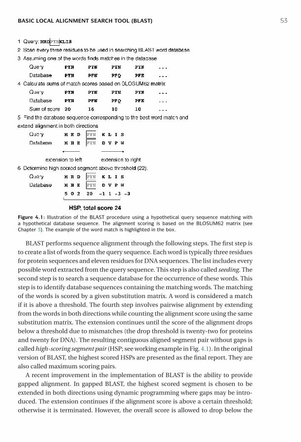
P1: JZP0521840988c04 CB1022/Xiong 0 521 84098 8 January 10, 2006 15:4
BASIC LOCAL ALIGNMENT SEARCH TOOL (BLAST) 53
Figure 4.1: Illustration of the BLAST procedure using a hypothetical query sequence matching witha hypothetical database sequence. The alignment scoring is based on the BLOSUM62 matrix (seeChapter 3). The example of the word match is highlighted in the box.
BLAST performs sequence alignment through the following steps. The first step isto create a list of words from the query sequence. Each word is typically three residuesfor protein sequences and eleven residues for DNA sequences. The list includes everypossible word extracted from the query sequence. This step is also called seeding. Thesecond step is to search a sequence database for the occurrence of these words. Thisstep is to identify database sequences containing the matching words. The matchingof the words is scored by a given substitution matrix. A word is considered a matchif it is above a threshold. The fourth step involves pairwise alignment by extendingfrom the words in both directions while counting the alignment score using the samesubstitution matrix. The extension continues until the score of the alignment dropsbelow a threshold due to mismatches (the drop threshold is twenty-two for proteinsand twenty for DNA). The resulting contiguous aligned segment pair without gaps iscalled high-scoring segment pair (HSP; see working example in Fig. 4.1). In the originalversion of BLAST, the highest scored HSPs are presented as the final report. They arealso called maximum scoring pairs.
A recent improvement in the implementation of BLAST is the ability to providegapped alignment. In gapped BLAST, the highest scored segment is chosen to beextended in both directions using dynamic programming where gaps may be intro-duced. The extension continues if the alignment score is above a certain threshold;otherwise it is terminated. However, the overall score is allowed to drop below the
P1: JZP0521840988c04 CB1022/Xiong 0 521 84098 8 January 10, 2006 15:4
54 DATABASE SIMILARITY SEARCHING
threshold only if it is temporary and rises again to attain above threshold values.Final trimming of terminal regions is needed before producing a report of the finalalignment.
Variants
BLAST is a family of programs that includes BLASTN, BLASTP, BLASTX TBLASTN,and TBLASTX. BLASTN queries nucleotide sequences with a nucleotide sequencedatabase. BLASTP uses protein sequences as queries to search against a proteinsequence database. BLASTX uses nucleotide sequences as queries and translatesthem in all six reading frames to produce translated protein sequences, which areused to query a protein sequence database. TBLASTN queries protein sequences to anucleotide sequence database with the sequences translated in all six reading frames.TBLASTX uses nucleotide sequences, which are translated in all six frames, to searchagainst a nucleotide sequence database that has all the sequences translated in sixframes. In addition, there is also a bl2seq program that performs local alignment oftwo user-provided input sequences. The graphical output includes horizontal barsand a diagonal in a two-dimensional diagram showing the overall extent of matchingbetween the two sequences.
The BLAST web server (www.ncbi.nlm.nih.gov/BLAST/) has been designed in sucha way as to simplify the task of program selection. The programs are organized based onthe type of query sequences, protein sequences, nucleotide sequences, or nucleotidesequence to be translated. In addition, programs for special purposes are groupedseparately; for example, bl2seq, immunoglobulin BLAST, and VecScreen, a program forremoving contaminating vector sequences. The BLAST programs specially designedfor searching individual genome databases are also listed in a separate category.
The choice of the type of sequences also influences the sensitivity of the search.Generally speaking, there is a clear advantage of using protein sequences in detectinghomologs. This is because DNA sequences only comprise four nucleotides, whereasprotein sequences contain twenty amino acids. This means that there is at least a five-fold increase in statistical complexity for protein sequences. More importantly, aminoacid substitution matrices incorporate subtle differences in physicochemical proper-ties between amino acids, meaning that protein sequences are far more informativeand sensitive in detection of homologs. This is why searches using protein sequencescan yield more significant matches than using DNA sequences. For that reason, if theinput sequence is a protein-encoding DNA sequence, it is preferable to use BLASTX,which translates it in six open reading frames before sequence comparisons arecarried out.
If one is looking for protein homologs encoded in newly sequenced genomes, onemay use TBLASTN, which translates nucleotide database sequences in all six openreading frames. This may help to identify protein coding genes that have not yet beenannotated. If a DNA sequence is to be used as the query, a protein-level comparison canbe done with TBLASTX. However, both programs are very computationally intensiveand the search process can be very slow.
P1: JZP0521840988c04 CB1022/Xiong 0 521 84098 8 January 10, 2006 15:4
BASIC LOCAL ALIGNMENT SEARCH TOOL (BLAST) 55
Statistical Significance
The BLAST output provides a list of pairwise sequence matches ranked by statis-tical significance. The significance scores help to distinguish evolutionarily relatedsequences from unrelated ones. Generally, only hits above a certain threshold aredisplayed.
Deriving the statistical measure is slightly different from that for single pairwisesequence alignment; the larger the database, the more unrelated sequence alignmentsthere are. This necessitates a new parameter that takes into account the total numberof sequence alignments conducted, which is proportional to the size of the database. InBLAST searches, this statistical indicator is known as the E-value (expectation value),and it indicates the probability that the resulting alignments from a database searchare caused by random chance. The E-value is related to the P-value used to assesssignificance of single pairwise alignment (see Chapter 3). BLAST compares a querysequence against all database sequences, and so the E-value is determined by thefollowing formula:
E = m × n × P (Eq. 4.1)
where m is the total number of residues in a database, n is the number of residuesin the query sequence, and P is the probability that an HSP alignment is a result ofrandom chance. For example, aligning a query sequence of 100 residues to a databasecontaining a total of 1012 residues results in a P-value for the ungapped HSP regionin one of the database matches of 1 × 1−20. The E-value, which is the product ofthe three values, is 100 × 1012 × 10−20, which equals 10−6. It is expressed as 1e − 6 inBLAST output. This indicates that the probability of this database sequence matchoccurring due to random chance is 10−6.
The E-value provides information about the likelihood that a given sequence matchis purely by chance. The lower the E-value, the less likely the database match is aresult of random chance and therefore the more significant the match is. Empiricalinterpretation of the E-value is as follows. If E < 1e − 50 (or 1 × 10−50), there shouldbe an extremely high confidence that the database match is a result of homologousrelationships. If E is between 0.01 and 1e − 50, the match can be considered a resultof homology. If E is between 0.01 and 10, the match is considered not significant, butmay hint at a tentative remote homology relationship. Additional evidence is neededto confirm the tentative relationship. If E > 10, the sequences under considerationare either unrelated or related by extremely distant relationships that fall below thelimit of detection with the current method.
Because the E-value is proportionally affected by the database size, an obviousproblem is that as the database grows, the E-value for a given sequence match alsoincreases. Because the genuine evolutionary relationship between the two sequencesremains constant, the decrease in credibility of the sequence match as the databasegrows means that one may “lose” previously detected homologs as the databaseenlarges. Thus, an alternative to E-value calculations is needed.
P1: JZP0521840988c04 CB1022/Xiong 0 521 84098 8 January 10, 2006 15:4
56 DATABASE SIMILARITY SEARCHING
A bit score is another prominent statistical indicator used in addition to the E-value in a BLAST output. The bit score measures sequence similarity independent ofquery sequence length and database size and is normalized based on the raw pairwisealignment score. The bit score (S ′) is determined by the following formula:
S ′ = (λ × S − lnK )/ ln2 (Eq. 4.2)
where λ is the Gumble distribution constant, S is the raw alignment score, and Kis a constant associated with the scoring matrix used. Clearly, the bit score (S ′) islinearly related to the raw alignment score (S). Thus, the higher the bit score, the morehighly significant the match is. The bit score provides a constant statistical indicatorfor searching different databases of different sizes or for searching the same databaseat different times as the database enlarges.
Low Complexity Regions
For both protein and DNA sequences, there may be regions that contain highly repeti-tive residues, such as short segments of repeats, or segments that are overrepresentedby a small number of residues. These sequence regions are referred to as low complex-ity regions (LCRs). LCRs are rather prevalent in database sequences; estimates indicatethat LCRs account for about 15% of the total protein sequences in public databases.These elements in query sequences can cause spurious database matches and leadto artificially high alignment scores with unrelated sequences.
To avoid the problem of high similarity scores owing to matching of LCRs thatobscure the real similarities, it is important to filter out the problematic regions inboth the query and database sequences to improve the signal-to-noise ratio, a pro-cess known as masking. There are two types of masking: hard and soft. Hard maskinginvolves replacing LCR sequences with an ambiguity character such as N fornucleotide residues or X for amino acid residues. The ambiguity characters are thenignored by the BLAST program, preventing the use of such regions in alignments andthus avoiding false positives. However, the drawback is that matching scores with truehomologs may be lowered because of shortened alignments. Soft masking involvesconverting the problematic sequences to lower case letters, which are ignored in con-structing the word dictionary, but are used in word extension and optimization ofalignments.
SEG is a program that is able to detect and mask repetitive elements before execut-ing database searches. It identifies LCRs by comparing residue frequencies of a certainregion with average residue frequencies in the database. If the residue frequencies ofa sequence region of the query sequence are significantly higher than the databaseaverage, the region is declared an LCR. SEG has been integrated into the BLAST web-based program. An option box for this low complexity filter needs to be selected tomask LCRs (either hard or soft masking).
RepeatMasker (http://woody.embl-heidelberg.de/repeatmask/) is an indepen-dent masking program that detects repetitive elements by comparing the query

P1: JZP0521840988c04 CB1022/Xiong 0 521 84098 8 January 10, 2006 15:4
FASTA 57
sequence with a built-in library of repetitive elements using the Smith–Watermanalgorithm. If the alignment score for a sequence region is above a certain threshold,the region is declared an LCR. The corresponding residues are then masked with N ’sor X ’s.
BLAST Output Format
The BLAST output includes a graphical overview box, a matching list and a text descrip-tion of the alignment (Fig. 4.2). The graphical overview box contains colored horizontalbars that allow quick identification of the number of database hits and the degrees ofsimilarity of the hits. The color coding of the horizontal bars corresponds to the rank-ing of similarities of the sequence hits (red: most related; green and blue: moderatelyrelated; black: unrelated). The length of the bars represents the spans of sequencealignments relative to the query sequence. Each bar is hyperlinked to the actual pair-wise alignment in the text portion of the report. Below the graphical box is a list ofmatching hits ranked by the E-values in ascending order. Each hit includes the acces-sion number, title (usually partial) of the database record, bit score, and E-value.
This list is followed by the text description, which may be divided into three sections:the header, statistics, and alignment. The header section contains the gene indexnumber or the reference number of the database hit plus a one-line description ofthe database sequence. This is followed by the summary of the statistics of the searchoutput, which includes the bit score, E-value, percentages of identity, similarity (“Pos-itives”), and gaps. In the actual alignment section, the query sequence is on the topof the pair and the database sequence is at the bottom of the pair labeled as Subject.In between the two sequences, matching identical residues are written out at theircorresponding positions, whereas nonidentical but similar residues are labeled with“+”. Any residues identified as LCRs in the query sequence are masked with Xs or Nsso that no alignment is represented in those regions.
FASTA
FASTA (FAST ALL, www.ebi.ac.uk/fasta33/) was in fact the first database similaritysearch tool developed, preceding the development of BLAST. FASTA uses a “hashing”strategy to find matches for a short stretch of identical residues with a length of k.The string of residues is known as ktuples or ktups, which are equivalent to words inBLAST, but are normally shorter than the words. Typically, a ktup is composed of tworesidues for protein sequences and six residues for DNA sequences.
The first step in FASTA alignment is to identify ktups between two sequences byusing the hashing strategy. This strategy works by constructing a lookup table thatshows the position of each ktup for the two sequences under consideration. The posi-tional difference for each word between the two sequences is obtained by subtractingthe position of the first sequence from that of the second sequence and is expressedas the offset. The ktups that have the same offset values are then linked to reveal a
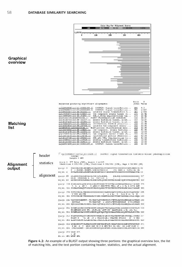
P1: JZP0521840988c04 CB1022/Xiong 0 521 84098 8 January 10, 2006 15:4
58 DATABASE SIMILARITY SEARCHING
Figure 4.2: An example of a BLAST output showing three portions: the graphical overview box, the listof matching hits, and the text portion containing header, statistics, and the actual alignment.
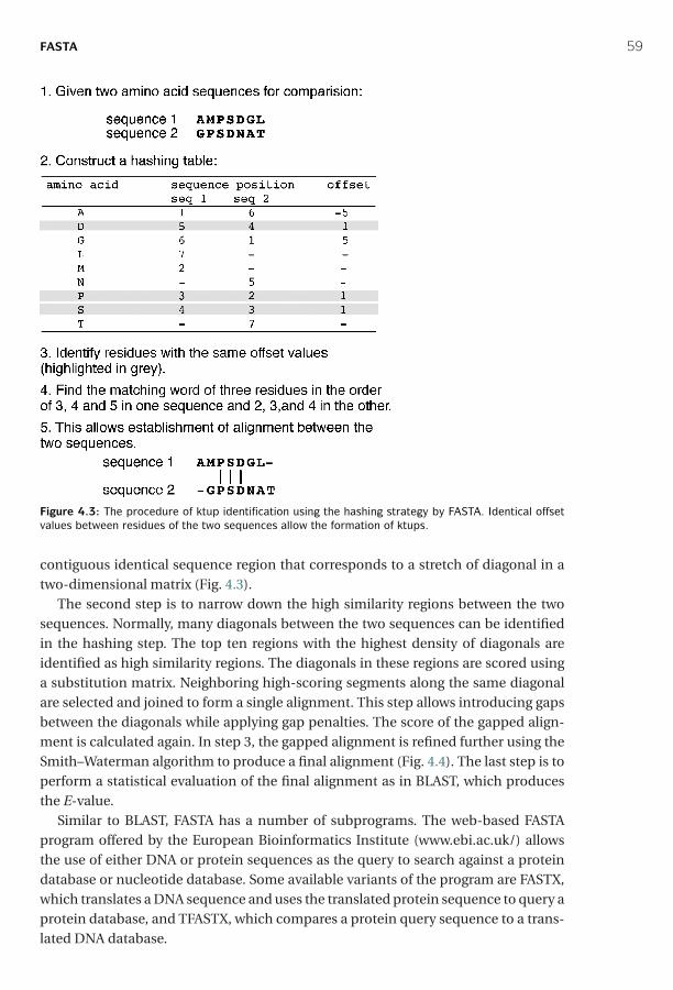
P1: JZP0521840988c04 CB1022/Xiong 0 521 84098 8 January 10, 2006 15:4
FASTA 59
Figure 4.3: The procedure of ktup identification using the hashing strategy by FASTA. Identical offsetvalues between residues of the two sequences allow the formation of ktups.
contiguous identical sequence region that corresponds to a stretch of diagonal in atwo-dimensional matrix (Fig. 4.3).
The second step is to narrow down the high similarity regions between the twosequences. Normally, many diagonals between the two sequences can be identifiedin the hashing step. The top ten regions with the highest density of diagonals areidentified as high similarity regions. The diagonals in these regions are scored usinga substitution matrix. Neighboring high-scoring segments along the same diagonalare selected and joined to form a single alignment. This step allows introducing gapsbetween the diagonals while applying gap penalties. The score of the gapped align-ment is calculated again. In step 3, the gapped alignment is refined further using theSmith–Waterman algorithm to produce a final alignment (Fig. 4.4). The last step is toperform a statistical evaluation of the final alignment as in BLAST, which producesthe E-value.
Similar to BLAST, FASTA has a number of subprograms. The web-based FASTAprogram offered by the European Bioinformatics Institute (www.ebi.ac.uk/) allowsthe use of either DNA or protein sequences as the query to search against a proteindatabase or nucleotide database. Some available variants of the program are FASTX,which translates a DNA sequence and uses the translated protein sequence to query aprotein database, and TFASTX, which compares a protein query sequence to a trans-lated DNA database.

P1: JZP0521840988c04 CB1022/Xiong 0 521 84098 8 January 10, 2006 15:4
60 DATABASE SIMILARITY SEARCHING
Figure 4.4: Steps of the FASTA alignment procedure. In step 1 (left ), all possible ungapped alignmentsare found between two sequences with the hashing method. In step 2 (middle), the alignments arescored according to a particular scoring matrix. Only the ten best alignments are selected. In step 3(right ), the alignments in the same diagonal are selected and joined to form a single gapped alignment,which is optimized using the dynamic programming approach.
Statistical Significance
FASTA also uses E-values and bit scores. Estimation of the two parameters in FASTAis essentially the same as in BLAST. However, the FASTA output provides one morestatistical parameter, the Z-score. This describes the number of standard deviationsfrom the mean score for the database search. Because most of the alignments with thequery sequence are with unrelated sequences, the higher the Z-score for a reportedmatch, the further away from the mean of the score distribution, hence, the moresignificant the match. For a Z-score > 15, the match can be considered extremelysignificant, with certainty of a homologous relationship. If Z is in the range of 5 to15, the sequence pair can be described as highly probable homologs. If Z < 5, theirrelationships is described as less certain.
COMPARISON OF FASTA AND BLAST
BLAST and FASTA have been shown to perform almost equally well in regular databasesearching. However, there are some notable differences between the two approaches.The major difference is in the seeding step; BLAST uses a substitution matrix to findmatching words, whereas FASTA identifies identical matching words using the hashingprocedure. By default, FASTA scans smaller window sizes. Thus, it gives more sensitiveresults than BLAST, with a better coverage rate for homologs. However, it is usuallyslower than BLAST. The use of low-complexity masking in the BLAST procedure meansthat it may have higher specificity than FASTA because potential false positives arereduced. BLAST sometimes gives multiple best-scoring alignments from the samesequence; FASTA returns only one final alignment.
P1: JZP0521840988c04 CB1022/Xiong 0 521 84098 8 January 10, 2006 15:4
SUMMARY 61
DATABASE SEARCHING WITH THE SMITH–WATERMAN METHOD
As mentioned, the rigorous dynamic programming method is normally not used fordatabase searching, because it is slow and computationally expensive. Heuristics suchas BLAST and FASTA are developed for faster speed. However, the heuristic methodsare limited in sensitivity and are not guaranteed to find the optimal alignment. Theyoften fail to find alignment for distantly related sequences. It has been estimatedthat for some families of protein sequences, BLAST can miss 30% of truly significanthits. Recent developments in computation technologies, such as parallel processingsupercomputers, have made dynamic programming a feasible approach to databasesearches to fill the performance gap.
For this purpose, the computer codes for the Needleman–Wunsch and Smith–Waterman algorithms have to be modified to run in a parallel processing environmentso that searches can be completed within reasonable time periods. Currently, thesearch speed is still slower than the popular heuristic programs. Therefore, the methodis not intended for routine use. Nevertheless, the availability of dynamic programmingallows the maximum sensitivity for finding homologs at the sequence level. Empiricaltests have indeed shown that the exhaustive method produces superior results overthe heuristic methods. Below is a list of dynamic programming-based web servers forsequence database searches.
ScanPS (Scan Protein Sequence, www.ebi.ac.uk/scanps/) is a web-based programthat implements a modified version of the Smith–Waterman algorithm optimized forparallel processing. The major feature is that the program allows iterative searchingsimilar to PSI-BLAST (see Chapter 5), which builds profiles from one round of searchresults and uses them for the second round of database searching. Full dynamic pro-gramming is used in each cycle for added sensitivity.
ParAlign (www.paralign.org/) is a web-based server that uses parallel processorsto perform exhaustive sequence comparisons using either a parallelized version ofthe Smith–Waterman algorithm or a heuristic program for further speed gains. Theheuristic subprogram first finds exact ungapped alignments and uses them as anchorsfor extension into gapped alignments by combining the scores of several diagonals inthe alignment matrix. The search speed of ParAlign approaches to that of BLAST, butwith higher sensitivity.
SUMMARY
Database similarity searching is an essential first step in the functional characteri-zation of novel gene or protein sequences. The major issues in database searchingare sensitivity, selectivity, and speed. Speed is a particular concern in searching largedatabases. Thus, heuristic methods have been developed for efficient database sim-ilarity searches. The major heuristic database searching algorithms are BLAST andFASTA. They both use a word method for pairwise alignment. BLAST looks for HSPs
P1: JZP0521840988c04 CB1022/Xiong 0 521 84098 8 January 10, 2006 15:4
62 DATABASE SIMILARITY SEARCHING
in a database. FASTA uses a hashing scheme to identify words. The major statisticalmeasures for significance of database matches are E-values and bit scores. A caveat forsequence database searching is to filter the LCRs using masking programs. Anothercaveat is to use protein sequences as the query in database searching, because theyproduce much more sensitive matches. In addition, it is important to keep in mindthat both BLAST and FASTA are heuristic programs and are not guaranteed to findall the homologous sequences. For significant matches automatically generated bythese programs, it is recommended to follow up the leads by checking the alignmentusing more rigorous and independent alignment programs. Advances in computa-tional technology have also made it possible to use full dynamic programming indatabase searching with increased sensitivity and selectivity.
FURTHER READING
Altschul, S. F., Boguski, M. S., Gish, W., and Wootton, J. C. 1994. Issues in searching molecularsequences databases. Nat. Genet. 6:119–29.
Altschul, S. F., Madden, T. L., Schaffer, A. A., Zhang, J., Zhang, Z., Miller, W., and Lipman, D. J.1997. Gapped BLAST and PSI-BLAST: A new generation of protein database search programs.Nucleic Acids Res. 25:3389–402.
Chen, Z. 2003. Assessing sequence comparison methods with the average precision criterion.Bioinformatics 19:2456–60.
Karlin, S., and Altschul, S. F. 1993. Applications and statistics for multiple high-scoring segmentsin molecular sequences. Proc. Natl. Acad. Sci. U S A 90:5873–7.
Mullan, L. J., and Williams, G. W. 2002. BLAST and go? Brief. Bioinform. 3:200–2.Sansom, C. 2000. Database searching with DNA and protein sequences: An introduction. Brief.
Bioinform. 1:22–32.Spang, R., and Vingron, M. 1998. Statistics of large-scale sequence searching. Bioinformatics
14:279–84.

P1: irk0521840988c05 CB1022/Xiong 0 521 84098 8 January 10, 2006 10:36
CHAPTER FIVE
Multiple Sequence Alignment
A natural extension of pairwise alignment is multiple sequence alignment, which isto align multiple related sequences to achieve optimal matching of the sequences.Related sequences are identified through the database similarity searching describedin Chapter 4. As the process generates multiple matching sequence pairs, it is oftennecessary to convert the numerous pairwise alignments into a single alignment, whicharranges sequences in such a way that evolutionarily equivalent positions across allsequences are matched.
There is a unique advantage of multiple sequence alignment because it revealsmore biological information than many pairwise alignments can. For example, itallows the identification of conserved sequence patterns and motifs in the wholesequence family, which are not obvious to detect by comparing only two sequences.Many conserved and functionally critical amino acid residues can be identified ina protein multiple alignment. Multiple sequence alignment is also an essential pre-requisite to carrying out phylogenetic analysis of sequence families and predictionof protein secondary and tertiary structures. Multiple sequence alignment also hasapplications in designing degenerate polymerase chain reaction (PCR) primers basedon multiple related sequences.
It is theoretically possible to use dynamic programming to align any number ofsequences as for pairwise alignment. However, the amount of computing time andmemory it requires increases exponentially as the number of sequences increases.As a consequence, full dynamic programming cannot be applied for datasets ofmore than ten sequences. In practice, heuristic approaches are most often used. Inthis chapter, methodologies and applications of multiple sequence alignment arediscussed.
SCORING FUNCTION
Multiple sequence alignment is to arrange sequences in such a way that a maximumnumber of residues from each sequence are matched up according to a particularscoring function. The scoring function for multiple sequence alignment is based onthe concept of sum of pairs (SP). As the name suggests, it is the sum of the scores ofall possible pairs of sequences in a multiple alignment based on a particular scoringmatrix. In calculating the SP scores, each column is scored by summing the scoresfor all possible pairwise matches, mismatches and gap costs. The score of the entire
63

P1: irk0521840988c05 CB1022/Xiong 0 521 84098 8 January 10, 2006 10:36
64 MULTIPLE SEQUENCE ALIGNMENT
Figure 5.1: Given a multiple alignment of three sequences,the sum of scores is calculated as the sum of the similarityscores of every pair of sequences at each position. The scor-ing is based on the BLOSUM62 matrix (see Chapter 3). Thetotal score for the alignment is 5, which means that the align-ment is 25 = 32 times more likely to occur among homologoussequences than by random chance.
alignment is the sum of all of the column scores (Fig. 5.1). The purpose of most multiplesequence alignment algorithms is to achieve maximum SP scores.
EXHAUSTIVE ALGORITHMS
As mentioned, there are exhaustive and heuristic approaches used in multiplesequence alignment. The exhaustive alignment method involves examining all pos-sible aligned positions simultaneously. Similar to dynamic programming in pairwisealignment, which involves the use of a two-dimensional matrix to search for an opti-mal alignment, to use dynamic programming for multiple sequence alignment, extradimensions are needed to take all possible ways of sequence matching into consid-eration. This means to establish a multidimensional search matrix. For instance, forthree sequences, a three-dimensional matrix is required to account for all possiblealignment scores. Back-tracking is applied through the three-dimensional matrix tofind the highest scored path that represents the optimal alignment. For aligning Nsequences, an N-dimensional matrix is needed to be filled with alignment scores. Asthe amount of computational time and memory space required increases exponen-tially with the number of sequences, it makes the method computationally prohibitiveto use for a large data set. For this reason, full dynamic programming is limited tosmall datasets of less than ten short sequences. For the same reason, few multiplealignment programs employing this “brute force” approach are publicly available. Aprogram called DCA, which uses some exhaustive components, is described below.
DCA (Divide-and-Conquer Alignment, http://bibiserv.techfak.uni-bielefeld.de/dca/) is a web-based program that is in fact semiexhaustive because certain stepsof computation are reduced to heuristics. It works by breaking each of the sequencesinto two smaller sections. The breaking points are determined based on regionalsimilarity of the sequences. If the sections are not short enough, further divisionsare carried out. When the lengths of the sequences reach a predefined threshold,dynamic programming is applied for aligning each set of subsequences. The result-ing short alignments are joined together head to tail to yield a multiple alignment ofthe entire length of all sequences. This algorithm provides an option of using a moreheuristic procedure (fastDCA) to choose optimal cutting points so it can more rapidlyhandle a greater number of sequences. It performs global alignment and requires theinput sequences to be of similar lengths and domain structures. Despite the use ofheuristics, the program is still extremely computationally intensive and can handleonly datasets of a very limited number of sequences.
P1: irk0521840988c05 CB1022/Xiong 0 521 84098 8 January 10, 2006 10:36
HEURISTIC ALGORITHMS 65
HEURISTIC ALGORITHMS
Because the use of dynamic programming is not feasible for routine multiple sequencealignment, faster and heuristic algorithms have been developed. The heuristic algo-rithms fall into three categories: progressive alignment type, iterative alignment type,and block-based alignment type. Each type of algorithm is described in turn.
Progressive Alignment Method
Progressive alignment depends on the stepwise assembly of multiple alignment and isheuristic in nature. It speeds up the alignment of multiple sequences through a multi-step process. It first conducts pairwise alignments for each possible pair of sequencesusing the Needleman–Wunsch global alignment method and records these similarityscores from the pairwise comparisons. The scores can either be percent identity orsimilarity scores based on a particular substitution matrix. Both scores correlate withthe evolutionary distances between sequences. The scores are then converted intoevolutionary distances to generate a distance matrix for all the sequences involved.A simple phylogenetic analysis is then performed based on the distance matrix togroup sequences based on pairwise distance scores. As a result, a phylogenetic treeis generated using the neighbor-joining method (see Chapter 11). The tree reflectsevolutionary proximity among all the sequences.
It needs to be emphasized that the resulting tree is an approximate tree and does nothave the rigor of a formally constructed phylogenetic tree (see Chapter 11). Nonethe-less, the tree can be used as a guide for directing realignment of the sequences. Forthat reason, it is often referred to as a guide tree. According to the guide tree, thetwo most closely related sequences are first re-aligned using the Needleman–Wunschalgorithm. To align additional sequences, the two already aligned sequences are con-verted to a consensus sequence with gap positions fixed. The consensus is then treatedas a single sequence in the subsequent step.
In the next step, the next closest sequence based on the guide tree is aligned withthe consensus sequence using dynamic programming. More distant sequences orsequence profiles are subsequently added one at a time in accordance with theirrelative positions on the guide tree. After realignment with a new sequence usingdynamic programming, a new consensus is derived, which is then used for the nextround of alignment. The process is repeated until all the sequences are aligned(Fig. 5.2).
Probably the most well-known progressive alignment program is Clustal. Some ofits important features are introduced next.
Clustal (www.ebi.ac.uk/clustalw/) is a progressive multiple alignment programavailable either as a stand-alone or on-line program. The stand-alone program, whichruns on UNIX and Macintosh, has two variants, ClustalW and ClustalX. The W versionprovides a simple text-based interface and the X version provides a more user-friendlygraphical interface.
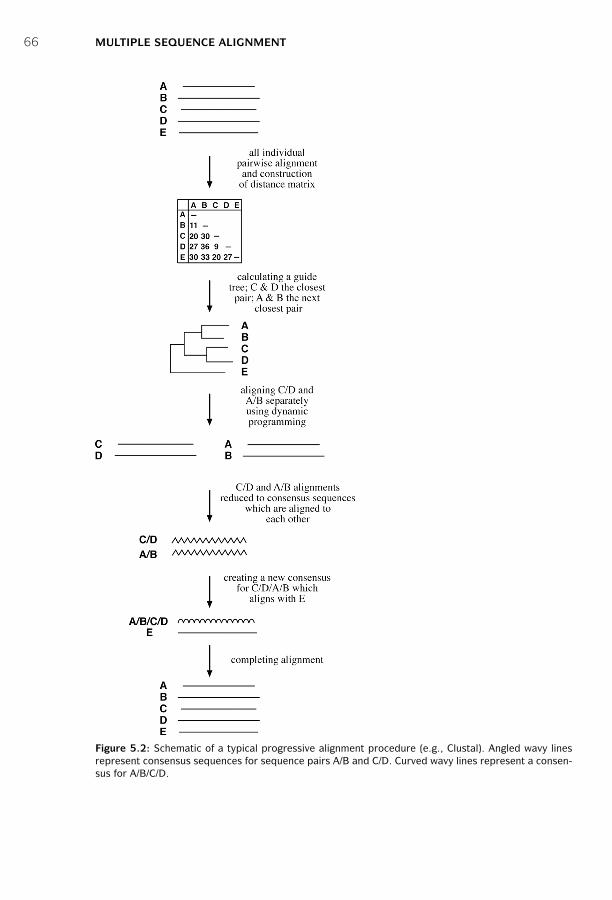
P1: irk0521840988c05 CB1022/Xiong 0 521 84098 8 January 10, 2006 10:36
66 MULTIPLE SEQUENCE ALIGNMENT
Figure 5.2: Schematic of a typical progressive alignment procedure (e.g., Clustal). Angled wavy linesrepresent consensus sequences for sequence pairs A/B and C/D. Curved wavy lines represent a consen-sus for A/B/C/D.
P1: irk0521840988c05 CB1022/Xiong 0 521 84098 8 January 10, 2006 10:36
HEURISTIC ALGORITHMS 67
One of the most important features of this program is the flexibility of using sub-stitution matrices. Clustal does not rely on a single substitution matrix. Instead, itapplies different scoring matrices when aligning sequences, depending on degrees ofsimilarity. The choice of a matrix depends on the evolutionary distances measuredfrom the guide tree. For example, for closely related sequences that are aligned inthe initial steps, Clustal automatically uses the BLOSUM62 or PAM120 matrix. Whenmore divergent sequences are aligned in later steps of the progressive alignment, theBLOSUM45 or PAM250 matrices may be used instead.
Another feature of Clustal is the use of adjustable gap penalties that allow moreinsertions and deletions in regions that are outside the conserved domains, but fewerin conserved regions. For example, a gap near a series of hydrophobic residues carriesmore penalties than the one next to a series of hydrophilic or glycine residues, whichare common in loop regions. In addition, gaps that are too close to one another canbe penalized more than gaps occurring in isolated loci.
The program also applies a weighting scheme to increase the reliability of aligningdivergent sequences (sequences with less than 25% identity). This is done by down-weighting redundant and closely related groups of sequences in the alignment by acertain factor. This scheme is useful in preventing similar sequences from dominatingthe alignment. The weight factor for each sequence is determined by its branch lengthon the guide tree. The branch lengths are normalized by how many times sequencesshare a basal branch from the root of the tree. The obtained value for each sequence issubsequently used to multiply the raw alignment scores of residues from that sequenceso to achieve the goal of decreasing the matching scores of frequent characters in amultiple alignment and thereby increasing the ones of infrequent characters.
Drawbacks and SolutionsThe progressive alignment method is not suitable for comparing sequences of differ-ent lengths because it is a global alignment–based method. As a result of the use ofaffine gap penalties (see Chapter 3), long gaps are not allowed, and, in some cases, thismay limit the accuracy of the method. The final alignment result is also influencedby the order of sequence addition. Another major limitation is the “greedy” natureof the algorithm: it depends on initial pairwise alignment. Once gaps introduced inthe early steps of alignment, they are fixed. Any errors made in these steps cannot becorrected. This problem of “once an error, always an error” can propagate throughoutthe entire alignment. In other words, the final alignment could be far from optimal.The problem can be more glaring when dealing with divergent sequences. To alleviatesome of the limitations, a new generation of algorithms have been developed, whichspecifically target some of the problems of the Clustal program.
T-Coffee (Tree-based Consistency Objective Function for alignment Evaluation;www.ch.embnet.org/software/TCoffee.html) performs progressive sequence align-ments as in Clustal. The main difference is that, in processing a query, T-Coffee per-forms both global and local pairwise alignment for all possible pairs involved. Theglobal pairwise alignment is performed using the Clustal program. The local pairwise
P1: irk0521840988c05 CB1022/Xiong 0 521 84098 8 January 10, 2006 10:36
68 MULTIPLE SEQUENCE ALIGNMENT
alignment is generated by the Lalign program, from which the top ten scored align-ments are selected. The collection of local and global sequence alignments are pooledto form a library. The consistency of the alignments is evaluated. For every pair ofresidues in a pair of sequences, a consistency score is calculated for both global andlocal alignments. Each pairwise alignment is further aligned with a possible thirdsequence. The result is used to refine the original pairwise alignment based on aconsistency criterion in a process known as library extension. Based on the refinedpairwise alignments, a distance matrix is built to derive a guide tree, which is thenused to direct a full multiple alignment using the progressive approach.
Because an optimal initial alignment is chosen from many alternative alignments,T-Coffee avoids the problem of getting stuck in the suboptimal alignment regions,which minimizes errors in the early stages of alignment assembly. Benchmark assess-ment has shown that T-Coffee indeed outperforms Clustal when aligning moderatelydivergent sequences. However, it is also slower than Clustal because of the extra com-puting time necessary for the calculation of consistency scores. T-Coffee providesa graphical output of the alignment results, with colored boxes to display degree ofagreement in the alignment library for various sequence regions.
DbClustal (http://igbmc.u-strasbg.fr:8080/DbClustal/dbclustal.html) is a Clustal-based database search algorithm for protein sequences that combines local and globalalignment features. It first performs a BLASTP search for a query sequence. The result-ing sequence alignment pairs above a certain threshold are analyzed to obtain anchorpoints, which are common conserved regions, by using a program called Ballast. Aglobal alignment is subsequently generated by Clustal, which is weighted toward theanchor points. Since the anchor points are derived from local alignments, this strategyminimizes errors caused by the global alignment. The resulting multiple alignmentis further evaluated by NorMD, which removes unrelated or badly aligned sequencesfrom the multiple alignment. Thus, the final alignment should be more accurate thanusing Clustal alone. It also allows the incorporation of very long gaps for insertionsand terminal extensions.
Poa (Partial order alignments, www.bioinformatics.ucla.edu/poa/) is a progressivealignment program that does not rely on guide trees. Instead, the multiple alignmentis assembled by adding sequences in the order they are given. Instead of using regularsequence consensus, a partial order graph is used to represent a growing multiplealignment, in which identical residues in a column are condensed to a node resem-bling a knot on a rope and divergent residues are allowed to remain as such, allowingthe rope to “bubble” (Fig. 5.3). The graph profile preserves all the information fromthe original alignment. Each time a new sequence is added, it is aligned with everysequence within the partial order graph individually using the Smith–Waterman algo-rithm. This allows the formation of a modified graph model, which is then used forthe next cycle of pairwise alignment. By building such a graph profile, the algorithmmaintains the information of the original sequences and eliminates the problem oferror fixation as in the Clustal alignment. Poa is local alignment-based and has beenshown to produce more accurate alignments than Clustal. Another advantage of this
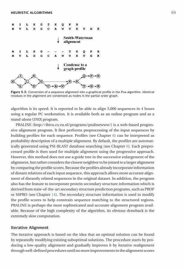
P1: irk0521840988c05 CB1022/Xiong 0 521 84098 8 January 10, 2006 10:36
HEURISTIC ALGORITHMS 69
Figure 5.3: Conversion of a sequence alignment into a graphical profile in the Poa algorithm. Identicalresidues in the alignment are condensed as nodes in the partial order graph.
algorithm is its speed. It is reported to be able to align 5,000 sequences in 4 hoursusing a regular PC workstation. It is available both as an online program and as astand-alone UNIX program.
PRALINE (http://ibivu.cs.vu.nl/programs/pralinewww/) is a web-based progres-sive alignment program. It first performs preprocessing of the input sequences bybuilding profiles for each sequence. Profiles (see Chapter 6) can be interpreted asprobability description of a multiple alignment. By default, the profiles are automat-ically generated using PSI-BLAST database searching (see Chapter 6). Each prepro-cessed profile is then used for multiple alignment using the progressive approach.However, this method does not use a guide tree in the successive enlargement of thealignment, but rather considers the closest neighbor to be joined to a larger alignmentby comparing the profile scores. Because the profiles already incorporate informationof distant relatives of each input sequence, this approach allows more accurate align-ment of distantly related sequences in the original dataset. In addition, the programalso has the feature to incorporate protein secondary structure information which isderived from state-of-the-art secondary structure prediction programs, such as PROFor SSPRO (see Chapter 14). The secondary structure information is used to modifythe profile scores to help constrain sequence matching to the structured regions.PRALINE is perhaps the most sophisticated and accurate alignment program avail-able. Because of the high complexity of the algorithm, its obvious drawback is theextremely slow computation.
Iterative Alignment
The iterative approach is based on the idea that an optimal solution can be foundby repeatedly modifying existing suboptimal solutions. The procedure starts by pro-ducing a low-quality alignment and gradually improves it by iterative realignmentthrough well-defined procedures until no more improvements in the alignment scores
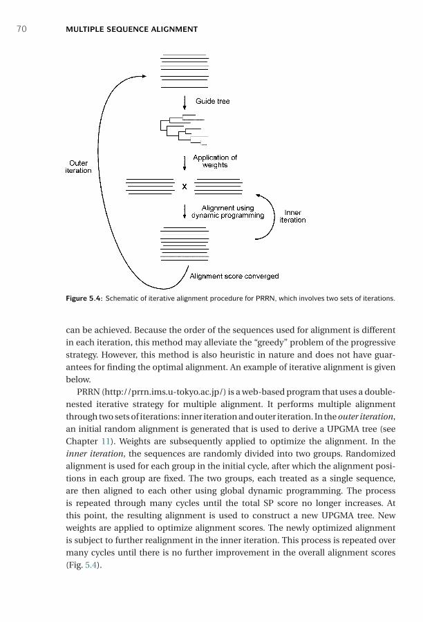
P1: irk0521840988c05 CB1022/Xiong 0 521 84098 8 January 10, 2006 10:36
70 MULTIPLE SEQUENCE ALIGNMENT
Figure 5.4: Schematic of iterative alignment procedure for PRRN, which involves two sets of iterations.
can be achieved. Because the order of the sequences used for alignment is differentin each iteration, this method may alleviate the “greedy” problem of the progressivestrategy. However, this method is also heuristic in nature and does not have guar-antees for finding the optimal alignment. An example of iterative alignment is givenbelow.
PRRN (http://prrn.ims.u-tokyo.ac.jp/) is a web-based program that uses a double-nested iterative strategy for multiple alignment. It performs multiple alignmentthrough two sets of iterations: inner iteration and outer iteration. In the outer iteration,an initial random alignment is generated that is used to derive a UPGMA tree (seeChapter 11). Weights are subsequently applied to optimize the alignment. In theinner iteration, the sequences are randomly divided into two groups. Randomizedalignment is used for each group in the initial cycle, after which the alignment posi-tions in each group are fixed. The two groups, each treated as a single sequence,are then aligned to each other using global dynamic programming. The processis repeated through many cycles until the total SP score no longer increases. Atthis point, the resulting alignment is used to construct a new UPGMA tree. Newweights are applied to optimize alignment scores. The newly optimized alignmentis subject to further realignment in the inner iteration. This process is repeated overmany cycles until there is no further improvement in the overall alignment scores(Fig. 5.4).
P1: irk0521840988c05 CB1022/Xiong 0 521 84098 8 January 10, 2006 10:36
PRACTICAL ISSUES 71
Block-Based Alignment
The progressive and iterative alignment strategies are largely global alignment basedand may therefore fail to recognize conserved domains and motifs (see Chapter 7)among highly divergent sequences of varying lengths. For such divergent sequencesthat share only regional similarities, a local alignment based approach has to be used.The strategy identifies a block of ungapped alignment shared by all the sequences,hence, the block-based local alignment strategy. Two block-based alignment pro-grams are introduced below.
DIALIGN2 (http://bioweb.pasteur.fr/seqanal/interfaces/dialign2.html) is a web-based program designed to detect local similarities. It does not apply gap penaltiesand thus is not sensitive to long gaps. The method breaks each of the sequences downto smaller segments and performs all possible pairwise alignments between the seg-ments. High-scoring segments, called blocks, among different sequences are thencompiled in a progressive manner to assemble a full multiple alignment. It placesemphasis on block-to-block comparison rather than residue-to-residue compari-son. The sequence regions between the blocks are left unaligned. The program hasbeen shown to be especially suitable for aligning divergent sequences with only localsimilarity.
Match-Box (www.sciences.fundp.ac.be/biologie/bms/matchbox submit.shtml) isa web-based server that also aims to identify conserved blocks (or boxes) amongsequences. The program compares segments of every nine residues of all possiblepairwise alignments. If the similarity of particular segments is above a certain thresh-old across all sequences, they are used as an anchor to assemble multiple alignments;residues between blocks are unaligned. The server requires the user to submit a set ofsequences in the FASTA format and the results are returned by e-mail.
PRACTICAL ISSUES
Protein-Coding DNA Sequences
As mentioned in the Chapter 4, alignment at the protein level is more sensitive thanat the DNA level. Sequence alignment directly at the DNA level can often result inframeshift errors because in DNA alignment gaps are introduced irrespective of codonboundaries. Therefore, in the process of achieving maximum sequence similarity atthe DNA level, mismatches of genetic codons occur that violate the accepted evolu-tionary scenario that insertions or deletions occur in units of codons. The resultingalignment can thus be biologically unrealistic. The example in Figure 5.5 shows howsuch errors can occur when two sequences are being compared at the protein andDNA levels.
For that reason, sequence alignment at the protein level is much more informativefor functional and evolutionary analysis. However, there are occasions when sequence

P1: irk0521840988c05 CB1022/Xiong 0 521 84098 8 January 10, 2006 10:36
72 MULTIPLE SEQUENCE ALIGNMENT
Figure 5.5: Comparison of alignment at the proteinlevel and DNA level. The DNA alignment on the leftis the correct one and consistent with amino acidsequence alignment, whereas the DNA alignment onthe right, albeit more optimal in matching similarresidues, is incorrect because it disregards the codonboundaries.
alignment at the DNA level is often necessary, for example, in designing PCR primersand in constructing DNA-based molecular phylogenetic trees.
Because conducting alignment directly at the DNA level often leads to errors, DNAcan be translated into an amino acid sequence before carrying out alignment to avoidthe errors of inserting gaps within codon boundaries. After alignment of the proteinsequences, the alignment can be converted back to DNA alignment while ensuringthat codons of the DNA sequences line up based on corresponding amino acids.The following are two web-based programs that allow easy conversion from proteinalignment to DNA alignment.
RevTrans (www.cbs.dtu.dk/services/RevTrans/) takes a set of DNA sequences,translates them, aligns the resulting protein sequences, and uses the protein align-ment as a scaffold for constructing the corresponding DNA multiple alignment. Italso allows the user to provide multiple protein alignment for greater control ofthe alignment process. PROTA2DNA (http://bioweb.pasteur.fr/seqanal/interfaces/protal2dna.html) aligns DNA sequences corresponding to a protein multiple align-ment.
Editing
No matter how good an alignment program seems, the automated alignment oftencontains misaligned regions. It is imperative that the user check the alignment care-fully for biological relevance and edit the alignment if necessary. This involves intro-ducing or removing gaps to maximize biologically meaningful matches. Sometimes,portions that are ambiguously aligned and deemed to be incorrect have to deleted.In manual editing, empirical evidence or mere experience is needed to make correc-tions on an alignment. One can simply use a word processor to edit the text-basedalignment. There are also dedicated software programs that assist in the process.
BioEdit (www.mbio.ncsu.edu/BioEdit/bioedit.html) is a multifunctional sequencealignment editor for Windows. It has a coloring scheme for nucleotide or amino acidresidues that facilitates manual editing. In addition, it is able to do BLAST searches,plasmid drawing, and restriction mapping.
P1: irk0521840988c05 CB1022/Xiong 0 521 84098 8 January 10, 2006 10:36
SUMMARY 73
Rascal (http://igbmc.u-strasbg.fr/PipeAlign/Rascal/rascal.html) is a web-basedprogram that automatically refines a multiple sequence alignment. It is part of thePipeAlign package. It is able to identify misaligned regions and realign them to improvethe quality of the alignment. It works by dividing the input alignment into severalregions horizontally and vertically to identify well-aligned and poorly aligned regionsusing an internal scoring scheme. Regions below certain thresholds are consideredmisaligned and are subsequently realigned using the progressive approach. The over-all quality of the alignment is then reassessed. If necessary, certain regions are furtherrealigned. The program also works in conjunction with NorMD, which validates therefined alignment and identifies potentially unrelated sequences for removal.
Format Conversion
In many bioinformatics analyses, in particular, phylogenetic analysis, it is often nec-essary to convert various formats of sequence alignments to the one acceptable byan application program. The task of format conversion requires a program to beable to read a multiple alignment in one format and rewrite it into another whilemaintaining the original alignment. This is a different task from simply convertingthe format of individual unaligned sequences. The BioEdit program mentioned isable to save an alignment in a variety of different formats. In addition, the Readseqprogram mentioned in Chapter 2 is able to perform format conversion of multiplealignment.
Readseq (http://iubio.bio.indiana.edu/cgi-bin/readseq.cgi/) is a web-based pro-gram that is able to do both simple sequence format conversion as well as alignmentformat conversions. The program can handle formats such as MSF, Phylip, Clustal,PAUP, and Pretty.
SUMMARY
Multiple sequence alignment is an essential technique in many bioinformatics appli-cations. Many algorithms have been developed to achieve optimal alignment. Someprograms are exhaustive in nature; some are heuristic. Because exhaustive programsare not feasible in most cases, heuristic programs are commonly used. These includeprogressive, iterative, and block-based approaches. The progressive method is a step-wise assembly of multiple alignment according to pairwise similarity. A prominentexample is Clustal, which is characterized by adjustable scoring matrices and gappenalties as well as by the application of weighting schemes. The major shortcomingof the program is its “greediness,” which relates to error fixation in the early steps ofcomputation. To remedy the problem, T-Coffee and DbClustal have been developedthat combine both global and local alignment to generate more sensitive alignment.Another improvement on the traditional progressive approach is to use graphic pro-files, as in Poa, which eliminate the problem of error fixation. Praline is profile basedand has the capacity to restrict alignment based on protein structure information andis thus much more accurate than Clustal. The iterative approach works by repetitive

P1: irk0521840988c05 CB1022/Xiong 0 521 84098 8 January 10, 2006 10:36
74 MULTIPLE SEQUENCE ALIGNMENT
refinement of suboptimal alignments. The block-based method focuses on identify-ing regional similarities. It is important to keep in mind that no alignment programis absolutely guaranteed to find correct alignment, especially when the number ofsequences is large and the divergence level is high. The alignment resulting fromautomated alignment programs often contains errors. The best approach is to performalignment using a combination of multiple alignment programs. The alignment resultcan be further refined manually or using Rascal. Protein-encoding DNA sequencesshould preferably be aligned at the protein level first, after which the alignment canbe converted back to DNA alignment.
FURTHER READING
Apostolico, A., and Giancarlo, R. 1998. Sequence alignment in molecular biology. J. Comput.Biol. 5:173–96.
Gaskell, G. J. 2000. Multiple sequence alignment tools on the Web. Biotechniques 29:60–2.Gotoh, O. 1999. Multiple sequence alignment: Algorithms and applications. Adv. Biophys.
36:159–206.Lecompte, O., Thompson, J. D., Plewniak, F., Thierry, J., and Poch, O. 2001. Multiple alignment
of complete sequences (MACS) in the post-genomic era. Gene 270:17–30.Morgenstern, B. 1999. DIALIGN 2: improvement of the segment-to-segment approach to
multiple sequence alignment. Bioinformatics 15:211–8.Morgenstern, B., Dress, A., and Werner T. 1996. Multiple DNA and protein sequence alignment
based on segment-to-segment comparison. Proc. Natl. Acad. Sci. U S A 93:12098–103.Mullan, L. J. 2002. Multiple sequence alignment – The gateway to further analysis. Brief.
Bioinform. 3:303–5.Nicholas, H. B. Jr., Ropelewski, A. J., and Deerfield, D. W. II. 2002. Strategies for multiple sequence
alignment. Biotechniques 32:572–91.Notredame, C. 2002. Recent progress in multiple sequence alignment: A survey. Pharmacoge-
nomics 3:131–44.Notredame, C., Higgins, D. G., and Heringa, J. 2000. T-Coffee: A novel method for fast and
accurate multiple sequence alignment. J. Mol. Biol. 302:205–17.Thompson, J. D., Higgins, D. G., and Gibson, T. J. 1994. CLUSTAL W: Improving the sensitivity of
progressive multiple sequence alignment through sequence weighting, position-specific gappenalties and weight matrix choice. Nucleic Acids Res. 22:4673–80.
Thompson, J. D., Plewniak, F., and Poch, O. 1999. A comprehensive comparison of multiplesequence alignment programs. Nucleic Acids Res. 27:2682–90.

P1: irk0521840988c06 CB1022/Xiong 0 521 84098 8 January 10, 2006 15:9
CHAPTER SIX
Profiles and Hidden Markov Models
One of the applications of multiple sequence alignments in identifying relatedsequences in databases is by construction of position-specific scoring matrices(PSSMs), profiles, and hidden Markov models (HMMs). These are statistical mod-els that reflect the frequency information of amino acid or nucleotide residues ina multiple alignment. Thus, they can be treated as consensus for a given sequencefamily. However, the “consensus” is not exactly a single sequence, but rather a modelthat captures not only the observed frequencies but also predicted frequencies ofunobserved characters. The purpose of establishing the mathematical models is toallow partial matches with a query sequence so they can be used to detect more dis-tant members of the same sequence family, resulting in an increased sensitivity ofdatabase searches. This chapter covers the basics of these statistical models followedby discussion of their applications.
POSITION-SPECIFIC SCORING MATRICES
A PSSM is defined as a table that contains probability information of amino acids ornucleotides at each position of an ungapped multiple sequence alignment. The matrixresembles the substitution matrices discussed in Chapter 3, but is more complex inthat it contains positional information of the alignment. In such a table, the rows rep-resent residue positions of a particular multiple alignment and the columns representthe names of residues or vice versa (Fig. 6.1). The values in the table represent log oddsscores of the residues calculated from the multiple alignment.
To construct a matrix, raw frequencies of each residue at each column position froma multiple alignment are first counted. The frequencies are normalized by dividingpositional frequencies of each residue by overall frequencies so that the scores arelength and composition independent. The values are converted to the probabilityvalues by taking to the logarithm (normally to the base of 2). In this way, the matrixvalues become log odds scores of residues occurring at each alignment position. Inthis matrix, a positive score represents identical residue or similar residue match; anegative score represents a nonconserved sequence match.
This constructed matrix can be considered a distilled representation for the entiregroup of related sequences, providing a quantitative description of the degree ofsequence conservation at each position of a multiple alignment. The probabilisticmodel can then be used like a single sequence for database searching and alignment
75

P1: irk0521840988c06 CB1022/Xiong 0 521 84098 8 January 10, 2006 15:9
76 PROFILES AND HIDDEN MARKOV MODELS
Figure 6.1: Example of construction of a PSSM from a multiple alignment of nucleotide sequences.The process involves counting raw frequencies of each nucleotide at each column position, normaliza-tion of the frequencies by dividing positional frequencies of each nucleotide by overall frequencies andconverting the values to log odds scores.
or can be used to test how well a particular target sequence fits into the sequencegroup.
For example, given the matrix shown in Figure 6.1, which is derived from a DNA mul-tiple alignment, one can ask the question, how well does the new sequence AACTCGfit into the matrix? To answer the question, the probability values of the sequence at
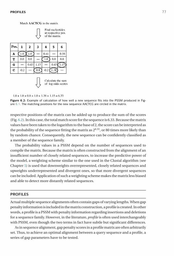
P1: irk0521840988c06 CB1022/Xiong 0 521 84098 8 January 10, 2006 15:9
PROFILES 77
Figure 6.2: Example of calculation of how well a new sequence fits into the PSSM produced in Fig-ure 6.1. The matching positions for the new sequence AACTCG are circled in the matrix.
respective positions of the matrix can be added up to produce the sum of the scores(Fig. 6.2). In this case, the total match score for the sequence is 6.33. Because the matrixvalues have been taken to the logarithm to the base of 2, the score can be interpreted asthe probability of the sequence fitting the matrix as 26.33, or 80 times more likely thanby random chance. Consequently, the new sequence can be confidently classified asa member of the sequence family.
The probability values in a PSSM depend on the number of sequences used tocompile the matrix. Because the matrix is often constructed from the alignment of aninsufficient number of closely related sequences, to increase the predictive power ofthe model, a weighting scheme similar to the one used in the Clustal algorithm (seeChapter 5) is used that downweights overrepresented, closely related sequences andupweights underrepresented and divergent ones, so that more divergent sequencescan be included. Application of such a weighting scheme makes the matrix less biasedand able to detect more distantly related sequences.
PROFILES
Actual multiple sequence alignments often contain gaps of varying lengths. When gappenalty information is included in the matrix construction, a profile is created. In otherwords, a profile is a PSSM with penalty information regarding insertions and deletionsfor a sequence family. However, in the literature, profile is often used interchangeablywith PSSM, even though the two terms in fact have subtle but significant differences.
As in sequence alignment, gap penalty scores in a profile matrix are often arbitrarilyset. Thus, to achieve an optimal alignment between a query sequence and a profile, aseries of gap parameters have to be tested.

P1: irk0521840988c06 CB1022/Xiong 0 521 84098 8 January 10, 2006 15:9
78 PROFILES AND HIDDEN MARKOV MODELS
Figure 6.3: Schematic diagram of PSI-BLAST, an iterative process used to identify distant homologs.
PSI-BLAST
Profiles can be used in database searching to find remote sequence homologs. How-ever, to manually construct a profile from a multiple alignment and calculate scores formatching sequences from a large database is tedious and involves significant exper-tise. It is desirable to have a program to establish profiles and use them to search againstsequence databases in an automated way. Such a program is fortunately available asPSI-BLAST, a variant of BLAST, provided by the National Center for BiotechnologyInformation.
Position-specific iterated BLAST (PSI-BLAST) builds profiles and performs data-base searches in an iterative fashion. It first uses a single query protein sequence toperform a normal BLASTP search to generate initial similarity hits. The high-scoringhits are used to build a multiple sequence alignment, from which a profile is created.The profile is then used in the second round of searching to identify more membersof the same family that may match with the profile. When new sequence hits areidentified, they are combined with the previous multiple alignment to generate a newprofile, which is in turn used in subsequent cycles of database searching. The processis repeated until no new sequence hits are found (Fig. 6.3).
The main feature of PSI-BLAST is that profiles are constructed automatically andare fine-tuned in each successive cycle. The program also employs a weighting schemein the profile construction in each iteration to increase sensitivity. Another measure

P1: irk0521840988c06 CB1022/Xiong 0 521 84098 8 January 10, 2006 15:9
MARKOV MODEL AND HIDDEN MARKOV MODEL 79
Figure 6.4: A simple representation of a Markov chain, which consists of a linear chain of events orstates (numbered) linked by transition probability values between events (states).
of PSI-BLAST to increase sensitivity is the use of pseudocounts (to be discussed next)to provide extra weight to unobserved residues to make the profile more inclusive.
The optimization of profile parameters makes PSI-BLAST a very sensitive searchstrategy to detect weak but biologically significant similarities between sequences.It has been estimated that the profile-based approach is able to identify three timesmore homologs than regular BLAST, which mainly fall within the range of less than30% sequence identity.
However, the high sensitivity of PSI-BLAST is also its pitfall; it is associated with lowselectivity caused by the false-positives generated in the automated profile construc-tion process. If unrelated sequences are erroneously included, profiles become biased.This allows further errors to be incorporated in subsequent cycles. This problem isknown as profile drift. A partial solution to this problem is to let the user visually inspectresults in each iteration and reject certain sequences that are known to be unrelatedbased on external knowledge. In addition, it is also prudent to conduct only a limitednumber of cycles instead of reaching full convergence. Typically, three to five iterationsof PSI-BLAST are sufficient to find most distant homologs at the sequence level.
MARKOV MODEL AND HIDDEN MARKOV MODEL
Markov Model
A more efficient way of computing matching scores between a sequence and asequence profile is through the use of HMMs, which are statistical models originallydeveloped for use in speech recognition. This statistical tool was subsequently foundto be ideal for describing sequence alignments. To understand HMMs, it is importantto have some general knowledge of Markov models.
A Markov model, also known as Markov chain, describes a sequence of eventsthat occur one after another in a chain. Each event determines the probability of thenext event (Fig. 6.4). A Markov chain can be considered as a process that moves inone direction from one state to the next with a certain probability, which is known astransition probability. A good example of a Markov model is the signal change of trafficlights in which the state of the current signal depends on the state of the previous signal(e.g., green light switches on after red light, which switches on after yellow light).
Biological sequences written as strings of letters can be described by Markov chainsas well; each letter representing a state is linked together with transitional probabilityvalues. The description of biological sequences using Markov chains allows the cal-culation of probability values for a given residue according to the unique distributionfrequencies of nucleotides or amino acids.
P1: irk0521840988c06 CB1022/Xiong 0 521 84098 8 January 10, 2006 15:9
80 PROFILES AND HIDDEN MARKOV MODELS
There are several different types of Markov models used to describe datasets ofdifferent complexities. In each type of Markov model, different mathematical solu-tions are derived. A zero-order Markov model describes the probability of the cur-rent state independent of the previous state. This is typical for a random sequence,in which every residue occurs with an equal frequency. A first-order Markov modeldescribes the probability of the current state being determined by the previous state.This corresponds to the unique frequencies of two linked residues (dimer) occur-ring simultaneously. Similarly, a second-order Markov model describes the situationin which the probability of the current state is determined by the previous two states.This corresponds to the unique trimer frequencies (three linked residues occurringsimultaneously as in the case of a codon) in biological sequences. For example, in aprotein-coding sequence, the frequency of unique trimers should be different fromthat in a noncoding or random sequence. This discrepancy can be described by thesecond-order Markov model. In addition, even higher orders of Markov models areavailable for biological sequence analysis (see Chapter 8).
Hidden Markov Model
In a Markov model, all states in a linear sequence are directly observable. In some sit-uations, some nonobserved factors influence state transition calculations. To includesuch factors in calculations requires the use of more sophisticated models: HMMs.An HMM combines two or more Markov chains with only one chain consisting ofobserved states and the other chains made up of unobserved (or “hidden”) states thatinfluence the outcome of the observed states (Fig. 6.5). For example, in a gapped align-ment, gaps do not correspond to any residues and are considered as unobservablestates. However, gaps indirectly influence the transition probability of the observedstates.
In an HMM, as in a Markov chain, the probability going from one state to anotherstate is the transition probability. Each state may be composed of a number elementsor symbols. For nucleotide sequences, there are four possible symbols – A, T, G, and C –in each state. For amino acid sequences, there twenty symbols. The probability valueassociated with each symbol in each state is called emission probability. To calculatethe total probability of a particular path of the model, both transition and emissionprobabilities linking all the “hidden” as well as observed states need to be taken intoaccount. Figure 6.6 provides a simple example of how to use two states of a partialHMM to represent (or generate) a sequence.
To develop a functional HMM that can be used to best represent a sequence align-ment, the statistical model has to be “trained,” which is a process to obtain the optimalstatistical parameters in the HMM. The training process involves calculation of thefrequencies of residues in each column in the multiple alignment built from a set ofrelated sequences. The frequency values are used to fill the emission and transitionprobability values in the model. Similar to the construction of a PSSM, once an HMMis established based on the training sequences, it can be used to determine how wellan unknown sequence matches the model.
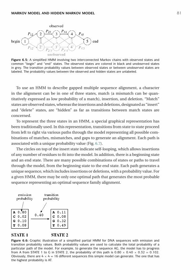
P1: irk0521840988c06 CB1022/Xiong 0 521 84098 8 January 10, 2006 15:9
MARKOV MODEL AND HIDDEN MARKOV MODEL 81
Figure 6.5: A simplified HMM involving two interconnected Markov chains with observed states andcommon “begin” and “end” states. The observed states are colored in black and unobserved statesin grey. The transition probability values between observed states or between unobserved states arelabeled. The probability values between the observed and hidden states are unlabeled.
To use an HMM to describe gapped multiple sequence alignment, a characterin the alignment can be in one of three states, match (a mismatch can be quan-titatively expressed as low probability of a match), insertion, and deletion. “Match”states are observed states, whereas the insertions and deletions, designated as “insert”and “delete” states, are “hidden” as far as transitions between match states areconcerned.
To represent the three states in an HMM, a special graphical representation hasbeen traditionally used. In this representation, transitions from state to state proceedfrom left to right via various paths through the model representing all possible com-binations of matches, mismatches, and gaps to generate an alignment. Each path isassociated with a unique probability value (Fig. 6.7).
The circles on top of the insert state indicate self-looping, which allows insertionsof any number of residues to fit into the model. In addition, there is a beginning stateand an end state. There are many possible combinations of states or paths to travelthrough the model, from the beginning state to the end state. Each path generates aunique sequence, which includes insertions or deletions, with a probability value. Fora given HMM, there may be only one optimal path that generates the most probablesequence representing an optimal sequence family alignment.
Figure 6.6: Graphic illustration of a simplified partial HMM for DNA sequences with emission andtransition probability values. Both probability values are used to calculate the total probability of aparticular path of the model. For example, to generate the sequence AG, the model has to progressfrom A from STATE 1 to G in STATE 2, the probability of this path is 0.80 × 0.40 × 0.32 = 0.102.Obviously, there are 4 × 4 = 16 different sequences this simple model can generate. The one that hasthe highest probability is AT.
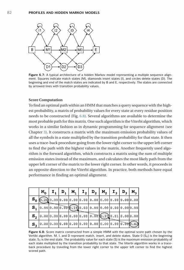
P1: irk0521840988c06 CB1022/Xiong 0 521 84098 8 January 10, 2006 15:9
82 PROFILES AND HIDDEN MARKOV MODELS
Figure 6.7: A typical architecture of a hidden Markov model representing a multiple sequence align-ment. Squares indicate match states (M), diamonds insert states (I), and circles delete states (D). Thebeginning and end of the match states are indicated by B and E, respectively. The states are connectedby arrowed lines with transition probability values.
Score ComputationTo find an optimal path within an HMM that matches a query sequence with the high-est probability, a matrix of probability values for every state at every residue positionneeds to be constructed (Fig. 6.8). Several algorithms are available to determine themost probable path for this matrix. One such algorithm is the Viterbi algorithm, whichworks in a similar fashion as in dynamic programming for sequence alignment (seeChapter 3). It constructs a matrix with the maximum emission probability values ofall the symbols in a state multiplied by the transition probability for that state. It thenuses a trace-back procedure going from the lower right corner to the upper left cornerto find the path with the highest values in the matrix. Another frequently used algo-rithm is the forward algorithm, which constructs a matrix using the sum of multipleemission states instead of the maximum, and calculates the most likely path from theupper left corner of the matrix to the lower right corner. In other words, it proceeds inan opposite direction to the Viterbi algorithm. In practice, both methods have equalperformance in finding an optimal alignment.
Figure 6.8: Score matrix constructed from a simple HMM with the optimal score path chosen by theVertibi algorithm. M, I, and D represent match, insert, and delete states. State 0 (S0) is the beginningstate; S3 is the end state. The probability value for each state (S) is the maximum emission probability ofeach state multiplied by the transition probability to that state. The Viterbi algorithm works in a trace-back procedure by traveling from the lower right corner to the upper left corner to find the highestscored path.
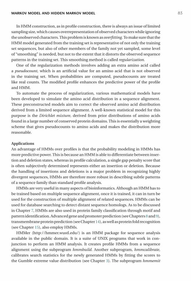
P1: irk0521840988c06 CB1022/Xiong 0 521 84098 8 January 10, 2006 15:9
MARKOV MODEL AND HIDDEN MARKOV MODEL 83
In HMM construction, as in profile construction, there is always an issue of limitedsampling size, which causes overrepresentation of observed characters while ignoringthe unobserved characters. This problem is known as overfitting. To make sure that theHMM model generated from the training set is representative of not only the trainingset sequences, but also of other members of the family not yet sampled, some levelof “smoothing” is needed, but not to the extent that it distorts the observed sequencepatterns in the training set. This smoothing method is called regularization.
One of the regularization methods involves adding an extra amino acid calleda pseudocount, which is an artificial value for an amino acid that is not observedin the training set. When probabilities are computed, pseudocounts are treatedlike real counts. The modified profile enhances the predictive power of the profileand HMM.
To automate the process of regularization, various mathematical models havebeen developed to simulate the amino acid distribution in a sequence alignment.These preconstructed models aim to correct the observed amino acid distributionderived from a limited sequence alignment. A well-known statistical model for thispurpose is the Dirichlet mixture, derived from prior distributions of amino acidsfound in a large number of conserved protein domains. This is essentially a weightingscheme that gives pseudocounts to amino acids and makes the distribution morereasonable.
ApplicationsAn advantage of HMMs over profiles is that the probability modeling in HMMs hasmore predictive power. This is because an HMM is able to differentiate between inser-tion and deletion states, whereas in profile calculation, a single gap penalty score thatis often subjectively determined represents either an insertion or deletion. Becausethe handling of insertions and deletions is a major problem in recognizing highlydivergent sequences, HMMs are therefore more robust in describing subtle patternsof a sequence family than standard profile analysis.
HMMs are very useful in many aspects of bioinformatics. Although an HMM has tobe trained based on multiple sequence alignment, once it is trained, it can in turn beused for the construction of multiple alignment of related sequences. HMMs can beused for database searching to detect distant sequence homologs. As to be discussedin Chapter 7, HMMs are also used in protein family classification through motif andpattern identification. Advanced gene and promoter prediction (see Chapters 8 and 9),transmembrane protein prediction (see Chapter 14), as well as protein fold recognition(see Chapter 15), also employ HMMs.
HMMer (http://hmmer.wustl.edu/) is an HMM package for sequence analysisavailable in the public domain. It is a suite of UNIX programs that work in con-junction to perform an HMM analysis. It creates profile HMMs from a sequencealignment using the subprogram hmmbuild. Another subprogram, hmmcalibrate,calibrates search statistics for the newly generated HMMs by fitting the scores tothe Gumble extreme value distribution (see Chapter 3). The subprogram hmmemit
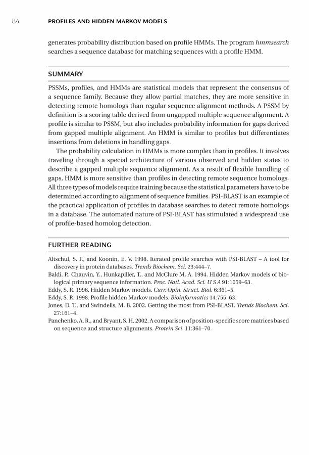
P1: irk0521840988c06 CB1022/Xiong 0 521 84098 8 January 10, 2006 15:9
84 PROFILES AND HIDDEN MARKOV MODELS
generates probability distribution based on profile HMMs. The program hmmsearchsearches a sequence database for matching sequences with a profile HMM.
SUMMARY
PSSMs, profiles, and HMMs are statistical models that represent the consensus ofa sequence family. Because they allow partial matches, they are more sensitive indetecting remote homologs than regular sequence alignment methods. A PSSM bydefinition is a scoring table derived from ungapped multiple sequence alignment. Aprofile is similar to PSSM, but also includes probability information for gaps derivedfrom gapped multiple alignment. An HMM is similar to profiles but differentiatesinsertions from deletions in handling gaps.
The probability calculation in HMMs is more complex than in profiles. It involvestraveling through a special architecture of various observed and hidden states todescribe a gapped multiple sequence alignment. As a result of flexible handling ofgaps, HMM is more sensitive than profiles in detecting remote sequence homologs.All three types of models require training because the statistical parameters have to bedetermined according to alignment of sequence families. PSI-BLAST is an example ofthe practical application of profiles in database searches to detect remote homologsin a database. The automated nature of PSI-BLAST has stimulated a widespread useof profile-based homolog detection.
FURTHER READING
Altschul, S. F., and Koonin, E. V. 1998. Iterated profile searches with PSI-BLAST – A tool fordiscovery in protein databases. Trends Biochem. Sci. 23:444–7.
Baldi, P., Chauvin, Y., Hunkapiller, T., and McClure M. A. 1994. Hidden Markov models of bio-logical primary sequence information. Proc. Natl. Acad. Sci. U S A 91:1059–63.
Eddy, S. R. 1996. Hidden Markov models. Curr. Opin. Struct. Biol. 6:361–5.Eddy, S. R. 1998. Profile hidden Markov models. Bioinformatics 14:755–63.Jones, D. T., and Swindells, M. B. 2002. Getting the most from PSI-BLAST. Trends Biochem. Sci.
27:161–4.Panchenko, A. R., and Bryant, S. H. 2002. A comparison of position-specific score matrices based
on sequence and structure alignments. Protein Sci. 11:361–70.

P1: JZP0521840988c07 CB1022/Xiong 0 521 84098 8 January 10, 2006 15:11
CHAPTER SEVEN
Protein Motif and Domain Prediction
An important aspect of biological sequence characterization is identification ofmotifs and domains. It is an important way to characterize unknown protein func-tions because a newly obtained protein sequence often lacks significant similar-ity with database sequences of known functions over their entire length, whichmakes functional assignment difficult. In this case, biologists can gain insight ofthe protein function based on identification of short consensus sequences relatedto known functions. These consensus sequence patterns are termed motifs anddomains.
A motif is a short conserved sequence pattern associated with distinct functionsof a protein or DNA. It is often associated with a distinct structural site perform-ing a particular function. A typical motif, such as a Zn-finger motif, is ten to twentyamino acids long. A domain is also a conserved sequence pattern, defined as an inde-pendent functional and structural unit. Domains are normally longer than motifs. Adomain consists of more than 40 residues and up to 700 residues, with an averagelength of 100 residues. A domain may or may not include motifs within its bound-aries. Examples of domains include transmembrane domains and ligand-bindingdomains.
Motifs and domains are evolutionarily more conserved than other regions of a pro-tein and tend to evolve as units, which are gained, lost, or shuffled as one module. Theidentification of motifs and domains in proteins is an important aspect of the clas-sification of protein sequences and functional annotation. Because of evolutionarydivergence, functional relationships between proteins often cannot be distinguishedthrough simple BLAST or FASTA database searches. In addition, proteins or enzymesoften perform multiple functions that cannot be fully described using a single anno-tation through sequence database searching. To resolve these issues, identification ofthe motifs and domains becomes very useful.
Identification of motifs and domains heavily relies on multiple sequence align-ment as well as profile and hidden Markov model (HMM) construction (see Chap-ters 5 and 6). This chapter focuses on some fundamental issues relating to proteinmotif and domain databases as well as classification of protein sequences using fulllength sequences. In addition, computational tools for discovering subtle motifs fromdivergent sequences are also introduced.
85
P1: JZP0521840988c07 CB1022/Xiong 0 521 84098 8 January 10, 2006 15:11
86 PROTEIN MOTIF AND DOMAIN PREDICTION
IDENTIFICATION OF MOTIFS AND DOMAINSIN MULTIPLE SEQUENCE ALIGNMENT
Motifs and domains are first constructed from multiple alignment of related sequ-ences. Based on the multiple sequence alignment, commonly conserved regions canbe identified. The regions considered motifs and domains then serve as diagnos-tic features for a protein family. The consensus sequence information of motifs anddomains can be stored in a database for later searches of the presence of similarsequence patterns from unknown sequences. By scanning the presence of knownmotifs or domains in a query sequence, associated functional features in a querysequence can be revealed rapidly, which is often not possible by simply matchingfull-length sequences in the primary databases.
There are generally two approaches to representing the consensus informationof motifs and domains. The first is to reduce the multiple sequence alignment fromwhich motifs or domains are derived to a consensus sequence pattern, known as aregular expression. For example, the protein phosphorylation motif can be expressedas [ST]-X-[RK]. The second approach is to use a statistical model such as a pro-file or HMM to include probability information derived from the multiple sequencealignment.
MOTIF AND DOMAIN DATABASES USING REGULAR EXPRESSIONS
A regular expression is a concise way of representing a sequence family by a string ofcharacters. When domains and motifs are written as regular expressions, the followingbasic rules to describe a sequence pattern are used: When a position is restricted to asingle conserved amino acid residue, it is indicated as such using the standard, one-letter code. When a position represents multiple alternative conserved residues, theresidues to be included are placed within brackets. If the position excludes certainresidues, residues to be excluded are placed in curly braces; nonspecific residuespresent in a given position in the pattern are indicated by an X; if a sequence elementwithin the pattern is repetitive, the number of pattern repetitions is indicated withinparentheses; and each position is linked by a hyphen. For example, a motif writtenas E-X(2)-[FHM]-X(4)-{P}-L can be interpreted as an E followed by two unspecificresidues which are followed by an F, or H or M residue which is followed by anotherfour unspecific residues followed by a non-P residue and a final L.
There are two mechanisms of matching regular expressions with a query sequence.One is exact matching and the other is fuzzy matching. In exact matching, there mustbe a strict match of sequence patterns. Any variations in the query sequence from thepredefined patterns are not allowed. Searching a motif database using this approachresults in either a match or nonmatch. This way of searching has a good chance ofmissing truly relevant motifs that have slight variations, thus generating false-negativeresults. Another limitation with using exact matching is that, as new sequences of a
P1: JZP0521840988c07 CB1022/Xiong 0 521 84098 8 January 10, 2006 15:11
MOTIF AND DOMAIN DATABASES USING STATISTICAL MODELS 87
motif are being accumulated, the rigid regular expression tends to become obsoleteif not updated regularly to reflect the changes.
Fuzzy matches, also called approximate matches, provide more permissive match-ing by allowing more flexible matching of residues of similar biochemical properties.For example, if an original alignment only contains phenylalanine at a particular posi-tion, fuzzy matching allows other aromatic residues (including unobserved tyrosineand tryptophan) in a sequence to match with the expression. This method is able toinclude more variant forms of a motif with a conserved function. However, associatedwith the more relaxed matching is the inevitable increase of the noise level and falsepositives. This is especially the case for short motifs. This is partly because the rule ofmatching is based on assumptions not actual observations.
Motif databases have commonly been used to classify proteins, provide functionalassignment, and identify structural and evolutionary relationships. Two databasesthat mainly employ regular expressions for the purpose of searching sequence pat-terns are described next.
PROSITE (www.expasy.ch/prosite/) is the first established sequence pattern data-base and is still widely used. It primarily uses a single consensus pattern or “sequencesignature” to characterize a protein function and a sequence family. The consensussequence patterns are derived from conserved regions of protein sequence alignmentsand are represented with regular expressions. The functional information of thesepatterns is primarily based on published literature. To search the database with aquery sequence, PROSITE uses exact matches to the sequence patterns. In additionto regular expressions, the database also constructs profiles to complement some ofthe sequence patterns. The major pitfall with the PROSITE patterns is that some of thesequence patterns are too short to be specific. The problem with these short sequencepatterns is that the resulting match is very likely to be a result of random events.Another problem is that the database is relatively small and motif searches often yieldno results when there are in fact true motif matches present (false negatives). Overall,PROSITE has a greater than 20% error rate. Thus, either a match or nonmatch inPROSITE should be treated with caution.
Emotif (http://motif.stanford.edu/emotif/emotif-search.html) is a motif databasethat uses multiple sequence alignments from both the BLOCKS and PRINTS databaseswith an alignment collection much larger than PROSITE. It identifies patterns byallowing fuzzy matching of regular expressions. Therefore, it produces fewer falsenegatives than PROSITE.
MOTIF AND DOMAIN DATABASES USING STATISTICAL MODELS
The major limitation of regular expressions is that this method does not take intoaccount sequence probability information about the multiple alignment from whichit is modeled. If a regular expression is derived from an incomplete sequence set, ithas less predictive power because many more sequences with the same type of motifsare not represented.
P1: JZP0521840988c07 CB1022/Xiong 0 521 84098 8 January 10, 2006 15:11
88 PROTEIN MOTIF AND DOMAIN PREDICTION
Unlike regular expressions, position-specific scoring matrices (PSSMs), profiles,and HMMs (see Chapter 6) preserve the sequence information from a multiplesequence alignment and express it with probabilistic models. In addition, these sta-tistical models allow partial matches and compensate for unobserved sequence pat-terns using pseudocounts. Thus, these statistical models have stronger predictivepower than the regular expression based approach, even when they are derived froma limited set of sequences. Using such a powerful scoring system can enhance thesensitivity of motif discovery and detect more divergent but truly related sequences.
The following programs mainly use the profile/HMM method extensively forsequence pattern construction.
PRINTS (http://bioinf.man.ac.uk/dbbrowser/PRINTS/) is a protein fingerprintdatabase containing ungapped, manually curated alignments corresponding to themost conserved regions among related sequences. This program breaks down a motifinto even smaller nonoverlapping units called fingerprints, which are represented byunweighted PSSMs. To define a motif, at least a majority of fingerprints are requiredto match with a query sequence. A query that has simultaneous high-scoring matchesto a majority of fingerprints belonging to a motif is a good indication of containingthe functional motif. The drawbacks of PRINTS are 1) the difficulty to recognize shortmotifs when they reach the size of single fingerprints and 2) a relatively small database,which restricts detection of many motifs.
BLOCKS (http://blocks.fhcrc.org/blocks) is a database that uses multiple align-ments derived from the most conserved, ungapped regions of homologous proteinsequences. The alignments are automatically generated using the same data sets usedfor deriving the BLOSUM matrices (see Chapter 3). The derived ungapped alignmentsare called blocks. The blocks, which are usually longer than motifs, are subsequentlyconverted to PSSMs. A weighting scheme and pseudocounts are subsequently appliedto the PSSMs to account for underrepresented and unobserved residues in align-ments. Because blocks often encompass motifs, the functional annotation of blocksis thus consistent with that for the motifs. A query sequence can be used to align withprecomputed profiles in the database to select the highest scored matches. Becauseof the use of the weighting scheme, the signal-to-noise ratio is improved relative toPRINTS.
ProDom (http://prodes.toulouse.inra.fr/prodom/2002.1/html/form.php) is a do-main database generated from sequences in the SWISSPROT and TrEMBL databases(see Chapter 2). The domains are built using recursive iterations of PSI-BLAST. Theautomatically generated sequence pattern database is designed to be an exhaustivecollection of domains without their functions necessarily being known.
Pfam (http://pfam.wustl.edu/hmmsearch.shtml) is a database with proteindomain alignments derived from sequences in SWISSPROT and TrEMBL. Each motifor domain is represented by an HMM profile generated from the seed alignment ofa number of conserved homologous proteins. Since the probability scoring mecha-nism is more complex in HMM than in a profile-based approach (see Chapter 6), the

P1: JZP0521840988c07 CB1022/Xiong 0 521 84098 8 January 10, 2006 15:11
MOTIF AND DOMAIN DATABASES USING STATISTICAL MODELS 89
use of HMM yields further increases in sensitivity of the database matches. The Pfamdatabase is composed of two parts, Pfam-A and Pfam-B. Pfam-A involves manualalignments and Pfam-B, automatic alignment in a way similar to ProDom. The func-tional annotation of motifs in Pfam-A is often related to that in PROSITE. Pfam-B onlycontains sequence families not covered in Pfam-A. Because of the automatic nature,Pfam-B has a much larger coverage but is also more error prone because some HMMsare generated from unrelated sequences.
SMART (Simple Modular Architecture Research Tool; http://smart.embl-heidelberg.de/) contains HMM profiles constructed from manually refined protein domainalignments. Alignments in the database are built based on tertiary structures when-ever available or based on PSI-BLAST profiles. Alignments are further checked andrefined by human annotators before HMM profile construction. Protein functions arealso manually curated. Thus, the database may be of better quality than Pfam withmore extensive functional annotations. Compared to Pfam, the SMART database con-tains an independent collection of HMMs, with emphasis on signaling, extracellular,and chromatin-associated motifs and domains. Sequence searching in this databaseproduces a graphical output of domains with well-annotated information with respectto cellular localization, functional sites, superfamily, and tertiary structure.
InterPro (www.ebi.ac.uk/interpro/) is an integrated pattern database designed tounify multiple databases for protein domains and functional sites. The database inte-grates information from PROSITE, Pfam, PRINTS, ProDom, and SMART databases.The sequence patterns from the five databases are further processed. Only overlappingmotifs and domains in a protein sequence derived by all five databases are included.The InterPro entries use a combination of regular expressions, fingerprints, profiles,and HMMs in pattern matching. However, an InterPro search does not obviate theneed to search other databases because of its unique criteria of motif inclusion andthus may have lower sensitivity than exhaustive searches in individual databases. Apopular feature of this database is a graphical output that summarizes motif matchesand has links to more detailed information.
Reverse PSI-BLAST (RPS-BLAST; www.ncbi.nlm.nih.gov/BLAST/) is a web-basedserver that uses a query sequence to search against a pre-computed profile databasegenerated by PSI-BLAST. This is opposite of PSI-BLAST that builds profiles frommatched database sequences, hence a “reverse” process. It performs only one itera-tion of regular BLAST searching against a database of PSI-BLAST profiles to find thehigh-scoring gapped matches.
CDART (Conserved Domain Architecture; www.ncbi.nlm.nih.gov/BLAST/) is a do-main search program that combines the results from RPS-BLAST, SMART, and Pfam.The resulting domain architecture of a query sequence can be graphically presentedalong with related sequences. The program is now an integral part of the regular BLASTsearch function. As with InterPro, CDART is not a substitute for individual databasesearches because it often misses certain features that can be found in SMART andPfam.

P1: JZP0521840988c07 CB1022/Xiong 0 521 84098 8 January 10, 2006 15:11
90 PROTEIN MOTIF AND DOMAIN PREDICTION
Caveats
Because of underlying differences in database construction and patten matchingmethods, each pattern database has its strengths and weaknesses. The coverage ofthese databases overlaps only to a certain extent. If a particular motif search returnsnothing from a particular database search, it does not mean that the sequence con-tains no patterns. It may be a result of the limited coverage of a particular databaseor an error in the database. Also keep in mind that there are many misannotatedsequences in databases, which hinder the detection of true motifs. Alternatively, thenonmatch may be a result of insensitive sequence matching methods. Therefore, itis advisable to use a combination of multiple databases in motif searching to get thegreatest coverage and consensus functional information. In cases of inconsistency ofresults when using several different databases, a majority rule can be a good way todiscriminate between the matches.
PROTEIN FAMILY DATABASES
The databases mentioned classify proteins based on the presence of motifs anddomains. Another way of classifying proteins is based on near full-length sequencecomparison. The latter classification scheme requires clustering of proteins basedon overall sequence similarities. The clustering criteria include statistical scores insequence alignments or orthologous relationships. Protein family databases derivedfrom this approach do not depend on the presence of particular sequence sig-natures and thus can be more comprehensive. However, the disadvantage is thatthere are more ambiguity and artifacts in protein classification. Two examples ofprotein family databases based on clustering and phylogenetic classification arepresented.
COG (Cluster of Orthologous Groups; www.ncbi.nlm.nih.gov/COG/) is a proteinfamily database based on phylogenetic classification. It is constructed by comparingprotein sequences encoded in forty-three completely sequenced genomes, which aremainly from prokaryotes, representing thirty major phylogenetic lineages. Throughall-against-all sequence comparisons among the genomes, orthologous proteinsshared by three or more lineages are identified and clustered together as orthologousgroups. Each group should have at least one representative from Archea, Bacteria,and Eukarya. Orthologs are included in a cluster as long as they satisfy the criterionof being the mutual best hits in BLAST searches among the genomes.
Because orthologous proteins shared by three or more lineages are considered tohave descended through a vertical evolutionary scenario, if the function of one ofthe members is known, functionality of other members can be assigned. Similarly,a query sequence can be assigned function if it has significant similarity matcheswith any member of the cluster. Currently, there are 4,873 clusters in the COGdatabases derived from unicellular organisms. The interface for sequence search-ing in the COG database is the COGnitor program, which is based on gapped
P1: JZP0521840988c07 CB1022/Xiong 0 521 84098 8 January 10, 2006 15:11
MOTIF DISCOVERY IN UNALIGNED SEQUENCES 91
BLAST. An eukaryotic version of the program is now available, known as KOG(www.ncbi.nlm.nih.gov/COG/new/kognitor.html).
ProtoNet (www.protonet.cs.huji.ac.il/) is a database of clusters of homologous pro-teins similar to COG. Orthologous protein sequences in the SWISSPROT databaseare clustered based on pairwise sequence comparisons between all possible proteinpairs using BLAST. Protein relatedness is defined by the E-values from the BLASTalignments. This produces different levels of protein similarity, yielding a hierarchicalorganization of protein groups. The most closely related sequences are grouped intothe lowest level clusters. More distant protein groups are merged into higher levelsof clusters. The outcome of this cluster merging is a tree-like structure of functionalcategories. A query protein sequence can be submitted to the server for cluster iden-tification and functional annotation. The database further provides gene ontologyinformation (see Chapter 16) for protein cluster at each level as well as keywords fromInterPro domains for functional prediction.
MOTIF DISCOVERY IN UNALIGNED SEQUENCES
For a set of closely related sequences, commonly shared motifs can be discoveredby using the multiple sequence alignment–based methods. Often, however, distantlyrelated sequences that share common motifs cannot be readily aligned. For exam-ple, the sequences for the helix-turn-helix motif in transcription factors can be sub-tly different enough that traditional multiple sequence alignment approaches fail togenerate a satisfactory answer. For detecting such subtle motifs, more sophisticatedalgorithms such as expectation maximization (EM) and Gibbs sampling are used.
Expectation Maximization
The EM procedure can be used to find hidden motifs using a method that is some-what different from profiles and PSSMs. The method works by first making a randomor guessed alignment of the sequences to generate a trial PSSM. The trial PSSM isthen used to compare with each sequence individually. The log odds scores of thePSSM are modified in each iteration to maximize the alignment of the matrix to eachsequence. During the iterations, the sequence pattern for the conserved motifs isgradually “recruited” to the PSSM (Fig. 7.1). The drawback of the EM method is thatthe procedure stops prematurely if the scores reach convergence, a problem knownas a local optimum. In addition, the final result is sensitive to the initial alignment.
Gibbs Motif Sampling
Another way to find conserved patterns from unaligned sequences is to use the Gibbssampling method. Similar to the EM method, the Gibbs sampling algorithm makes aninitial guessed alignment of all but one sequence. A trial PSSM is built to represent thealignment. The matrix is then aligned to the left-out sequence. The matrix scores aresubsequently adjusted to achieve the best alignment with the left-out sequence. Thisprocess is repeated many times until there is no further improvement on the matrix

P1: JZP0521840988c07 CB1022/Xiong 0 521 84098 8 January 10, 2006 15:11
92 PROTEIN MOTIF AND DOMAIN PREDICTION
Figure 7.1: Schematic diagram of the EM algorithm.
scores. The end result is that after a number of iterations, the most probable patternscan be incorporated into a final PSSM. This procedure is less susceptible to prematuretermination due to the local optimum problem.
MEME (Multiple EM for motif elicitation, http://meme.sdsc.edu/meme/website/meme-intro.html) is a web-based program that uses the EM algorithm to find motifseither for DNA or protein sequences. It uses a modified EM algorithm to avoid the localminimum problem. In constructing a probability matrix, it allows multiple startingalignments and does not assume that there are motifs in every sequence. The com-putation is a two-step procedure. In the first step, the user provides approximately 20unaligned sequences. The program applies EM to generate a sequence motif, which isan ungapped local sequence alignment. In the second step, segments from the querysequences with the same length as the motif are reapplied with the EM procedure tooptimize the alignment between the subsequences and the motif. A segment with thehighest score from the second iteration is selected as the optimum motif.
Gibbs sampler (http://bayesweb.wadsworth.org/gibbs/gibbs.html) is a web-basedprogram that uses the Gibbs sampling approach to look for short, partially conservedgap-free segments for either DNA or protein sequences. To ensure accuracy, morethan twenty sequences of the exact same length should be used.
SEQUENCE LOGOS
A multiple sequence alignment or a motif is often represented by a graphic represen-tation called a logo. In a logo, each position consists of stacked letters representing theresidues appearing in a particular column of a multiple alignment (Fig. 7.2). The over-all height of a logo position reflects how conserved the position is, and the height of
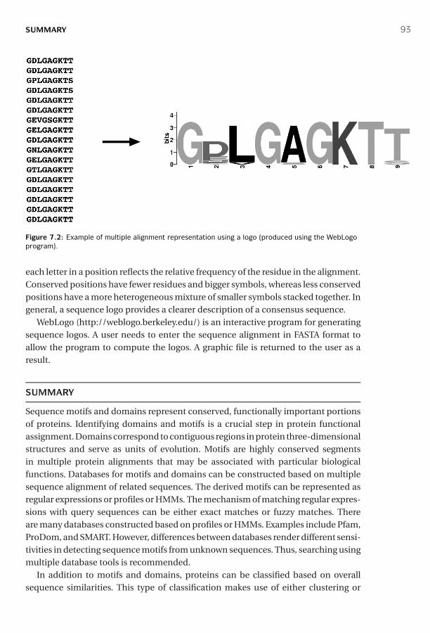
P1: JZP0521840988c07 CB1022/Xiong 0 521 84098 8 January 10, 2006 15:11
SUMMARY 93
Figure 7.2: Example of multiple alignment representation using a logo (produced using the WebLogoprogram).
each letter in a position reflects the relative frequency of the residue in the alignment.Conserved positions have fewer residues and bigger symbols, whereas less conservedpositions have a more heterogeneous mixture of smaller symbols stacked together. Ingeneral, a sequence logo provides a clearer description of a consensus sequence.
WebLogo (http://weblogo.berkeley.edu/) is an interactive program for generatingsequence logos. A user needs to enter the sequence alignment in FASTA format toallow the program to compute the logos. A graphic file is returned to the user as aresult.
SUMMARY
Sequence motifs and domains represent conserved, functionally important portionsof proteins. Identifying domains and motifs is a crucial step in protein functionalassignment. Domains correspond to contiguous regions in protein three-dimensionalstructures and serve as units of evolution. Motifs are highly conserved segmentsin multiple protein alignments that may be associated with particular biologicalfunctions. Databases for motifs and domains can be constructed based on multiplesequence alignment of related sequences. The derived motifs can be represented asregular expressions or profiles or HMMs. The mechanism of matching regular expres-sions with query sequences can be either exact matches or fuzzy matches. Thereare many databases constructed based on profiles or HMMs. Examples include Pfam,ProDom, and SMART. However, differences between databases render different sensi-tivities in detecting sequence motifs from unknown sequences. Thus, searching usingmultiple database tools is recommended.
In addition to motifs and domains, proteins can be classified based on overallsequence similarities. This type of classification makes use of either clustering or
P1: JZP0521840988c07 CB1022/Xiong 0 521 84098 8 January 10, 2006 15:11
94 PROTEIN MOTIF AND DOMAIN PREDICTION
phylogenetic algorithms. Some examples are COG and ProtoNet. They are powerfultools in functional annotation of new protein sequences. Subtle motifs from divergentsequences can be discovered using the EM and Gibbs sampling approaches. Sequencelogos are an effective way to represent motifs.
FURTHER READING
Attwood, T. K. 2000. The quest to deduce protein function from sequence: The role of patterndatabases. Int. J. Biochem. Cell. Biol. 32:139–55.
Attwood, T. K. 2002. The PRINTS database: A resource for identification of protein families. Brief.Bioinform. 3:252–63.
Biswas, M., O’Rourke, J. F., Camon, E., Fraser, G., Kanapin, A., Karavidopoulou, Y., Kersey, P.,et al. Applications of InterPro in protein annotation and genome analysis. Brief. Bioinform.3:285–95.
Copley, R. R., Ponting, C. P., Schultz, J., and Bork, P. 2002. Sequence analysis of multidomainproteins: Past perspectives and future directions. Adv. Protein Chem. 61:75–98.
Kanehisa, M., and Bork, P. 2003. Bioinformatics in the post-sequence era. Nat. Genet. 33 (Suppl):305–10.
Kong, L., and Ranganathan, S. 2004. Delineation of modular proteins: Domain boundary pre-diction from sequence information. Brief. Bioinform. 5:179–92.
Kriventseva, E. V., Biswas, M., and Apweiler R. 2001. Clustering and analysis of protein families.Curr. Opin. Struct. Biol. 11:334–9.
Liu, J., and Rost, B. 2003. Domains, motifs and clusters in the protein universe. Curr. Opin. Chem.Biol. 7:5–11.
Peri, S., Ibarrola, N., Blagoev, B., Mann, M., and Pandey, A. 2001. Common pitfalls inbioinformatics-based analyses: Look before you leap. Trends Genet. 17:541–5.
Servant, F., Bru, C., Carrere, S., Courcelle, E., Gouzy, J., Peyruc, D., and Kahn, D. 2002. ProDom:Automated clustering of homologous domains. Brief. Bioinform. 3:246–51.
Sigrist, C. J., Cerutti, L., Hulo, N., Gattiker, A., Falquet, L., Pagni, M., Bairoch, A., and Bucher,P. 2002. PROSITE: A documented database using patterns and profiles as motif descriptors.Brief. Bioinform. 3:265–74.
Wu, C. H., Huang, H., Yeh, L. S., and Barker, W. C. 2003. Protein family classification and functionalannotation. Comput. Biol. Chem. 27:37–47.

P1: JZP0521840988c08 CB1022/Xiong 0 521 84098 8 January 10, 2006 10:51
SECTION THREE
Gene and Promoter Prediction
95

P1: JZP0521840988c08 CB1022/Xiong 0 521 84098 8 January 10, 2006 10:51
96
P1: JZP0521840988c08 CB1022/Xiong 0 521 84098 8 January 10, 2006 10:51
CHAPTER EIGHT
Gene Prediction
With the rapid accumulation of genomic sequence information, there is a pressingneed to use computational approaches to accurately predict gene structure. Compu-tational gene prediction is a prerequisite for detailed functional annotation of genesand genomes. The process includes detection of the location of open reading frames(ORFs) and delineation of the structures of introns as well as exons if the genes ofinterest are of eukaryotic origin. The ultimate goal is to describe all the genes com-putationally with near 100% accuracy. The ability to accurately predict genes cansignificantly reduce the amount of experimental verification work required.
However, this may still be a distant goal, particularly for eukaryotes, because manyproblems in computational gene prediction are still largely unsolved. Gene prediction,in fact, represents one of the most difficult problems in the field of pattern recognition.This is because coding regions normally do not have conserved motifs. Detectingcoding potential of a genomic region has to rely on subtle features associated withgenes that may be very difficult to detect.
Through decades of research and development, much progress has been made inprediction of prokaryotic genes. A number of gene prediction algorithms for prokary-otic genomes have been developed with varying degrees of success. Algorithms foreukarytotic gene prediction, however, are still yet to reach satisfactory results. Thischapter describes a number of commonly used prediction algorithms, their theoret-ical basis, and limitations. Because of the significant differences in gene structuresof prokaryotes and eukaryotes, gene prediction for each group of organisms is dis-cussed separately. In addition, because of the predominance of protein coding genesin a genome (as opposed to rRNA and tRNA genes), the discussion focuses on theprediction of protein coding sequences.
CATEGORIES OF GENE PREDICTION PROGRAMS
The current gene prediction methods can be classified into two major categories, abinitio–based and homology-based approaches. The ab initio–based approach predictsgenes based on the given sequence alone. It does so by relying on two major featuresassociated with genes. The first is the existence of gene signals, which include start andstop codons, intron splice signals, transcription factor binding sites, ribosomal bind-ing sites, and polyadenylation (poly-A) sites. In addition, the triplet codon structurelimits the coding frame length to multiples of three, which can be used as a conditionfor gene prediction. The second feature used by ab initio algorithms is gene content,
97
P1: JZP0521840988c08 CB1022/Xiong 0 521 84098 8 January 10, 2006 10:51
98 GENE PREDICTION
which is statistical description of coding regions. It has been observed that nucleotidecomposition and statistical patterns of the coding regions tend to vary significantlyfrom those of the noncoding regions. The unique features can be detected by employ-ing probabilistic models such as Markov models or hidden Markov models (HMMs;see Chapter 6) to help distinguish coding from noncoding regions.
The homology-based method makes predictions based on significant matches ofthe query sequence with sequences of known genes. For instance, if a translated DNAsequence is found to be similar to a known protein or protein family from a databasesearch, this can be strong evidence that the region codes for a protein. Alternatively,when possible exons of a genomic DNA region match a sequenced cDNA, this alsoprovides experimental evidence for the existence of a coding region.
Some algorithms make use of both gene-finding strategies. There are also a num-ber of programs that actually combine prediction results from multiple individualprograms to derive a consensus prediction. This type of algorithms can therefore beconsidered as consensus based.
GENE PREDICTION IN PROKARYOTES
Prokaryotes, which include bacteria and Archaea, have relatively small genomes withsizes ranging from 0.5 to 10 Mbp (1 Mbp = 106 bp). The gene density in the genomes ishigh, with more than 90% of a genome sequence containing coding sequence. Thereare very few repetitive sequences. Each prokaryotic gene is composed of a singlecontiguous stretch of ORF coding for a single protein or RNA with no interruptionswithin a gene.
More detailed knowledge of the bacterial gene structure can be very useful in geneprediction. In bacteria, the majority of genes have a start codon ATG (or AUG in mRNA;because prediction is done at the DNA level, T is used in place of U), which codes formethionine. Occasionally, GTG and TTG are used as alternative start codons, butmethionine is still the actual amino acid inserted at the first position. Because theremay be multiple ATG, GTG, or TGT codons in a frame, the presence of these codons atthe beginning of the frame does not necessarily give a clear indication of the translationinitiation site. Instead, to help identify this initiation codon, other features associatedwith translation are used. One such feature is the ribosomal binding site, also called theShine-Delgarno sequence, which is a stretch of purine-rich sequence complementaryto 16S rRNA in the ribosome (Fig. 8.1). It is located immediately downstream of thetranscription initiation site and slightly upstream of the translation start codon. Inmany bacteria, it has a consensus motif of AGGAGGT. Identification of the ribosomebinding site can help locate the start codon.
At the end of the protein coding region is a stop codon that causes translation tostop. There are three possible stop codons, identification of which is straightfor-ward. Many prokaryotic genes are transcribed together as one operon. The end of theoperon is characterized by a transcription termination signal called ρ-independentterminator. The terminator sequence has a distinct stem-loop secondary structure
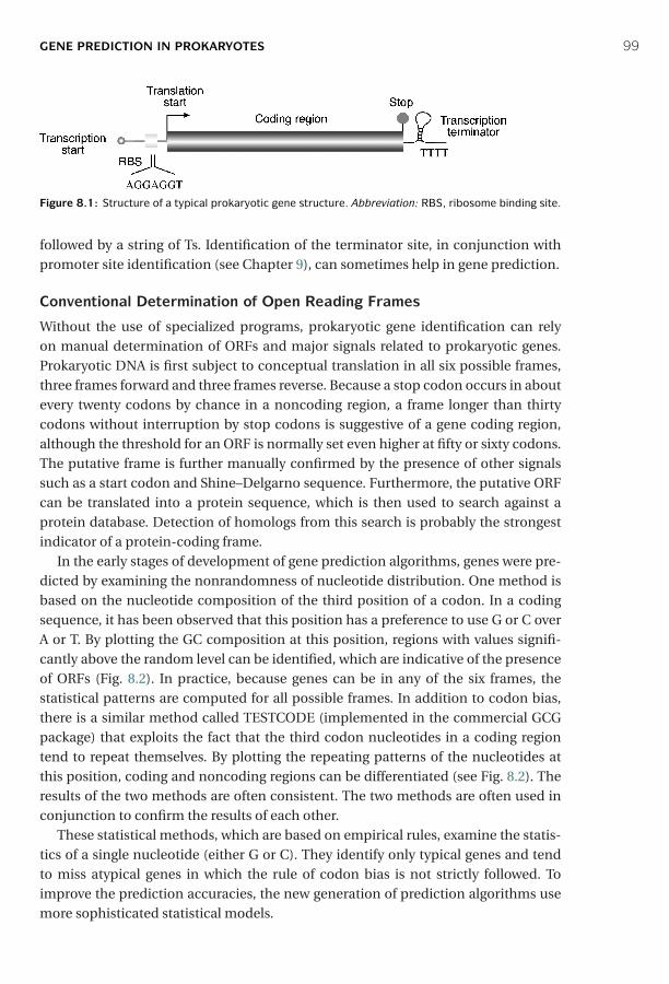
P1: JZP0521840988c08 CB1022/Xiong 0 521 84098 8 January 10, 2006 10:51
GENE PREDICTION IN PROKARYOTES 99
Figure 8.1: Structure of a typical prokaryotic gene structure. Abbreviation: RBS, ribosome binding site.
followed by a string of Ts. Identification of the terminator site, in conjunction withpromoter site identification (see Chapter 9), can sometimes help in gene prediction.
Conventional Determination of Open Reading Frames
Without the use of specialized programs, prokaryotic gene identification can relyon manual determination of ORFs and major signals related to prokaryotic genes.Prokaryotic DNA is first subject to conceptual translation in all six possible frames,three frames forward and three frames reverse. Because a stop codon occurs in aboutevery twenty codons by chance in a noncoding region, a frame longer than thirtycodons without interruption by stop codons is suggestive of a gene coding region,although the threshold for an ORF is normally set even higher at fifty or sixty codons.The putative frame is further manually confirmed by the presence of other signalssuch as a start codon and Shine–Delgarno sequence. Furthermore, the putative ORFcan be translated into a protein sequence, which is then used to search against aprotein database. Detection of homologs from this search is probably the strongestindicator of a protein-coding frame.
In the early stages of development of gene prediction algorithms, genes were pre-dicted by examining the nonrandomness of nucleotide distribution. One method isbased on the nucleotide composition of the third position of a codon. In a codingsequence, it has been observed that this position has a preference to use G or C overA or T. By plotting the GC composition at this position, regions with values signifi-cantly above the random level can be identified, which are indicative of the presenceof ORFs (Fig. 8.2). In practice, because genes can be in any of the six frames, thestatistical patterns are computed for all possible frames. In addition to codon bias,there is a similar method called TESTCODE (implemented in the commercial GCGpackage) that exploits the fact that the third codon nucleotides in a coding regiontend to repeat themselves. By plotting the repeating patterns of the nucleotides atthis position, coding and noncoding regions can be differentiated (see Fig. 8.2). Theresults of the two methods are often consistent. The two methods are often used inconjunction to confirm the results of each other.
These statistical methods, which are based on empirical rules, examine the statis-tics of a single nucleotide (either G or C). They identify only typical genes and tendto miss atypical genes in which the rule of codon bias is not strictly followed. Toimprove the prediction accuracies, the new generation of prediction algorithms usemore sophisticated statistical models.

P1: JZP0521840988c08 CB1022/Xiong 0 521 84098 8 January 10, 2006 10:51
100 GENE PREDICTION
Figure 8.2: Coding frame detection of a bacterial gene using either the GC bias or the TESTCODEmethod. Both result in similar identification of a reading frame (dashed arrows).
Gene Prediction Using Markov Models and Hidden Markov Models
Markov models and HMMs can be very helpful in providing finer statistical descriptionof a gene (see Chapter 6). A Markov model describes the probability of the distributionof nucleotides in a DNA sequence, in which the conditional probability of a particularsequence position depends on k previous positions. In this case, k is the order of aMarkov model. A zero-order Markov model assumes each base occurs independentlywith a given probability. This is often the case for noncoding sequences. A first-orderMarkov model assumes that the occurrence of a base depends on the base precedingit. A second-order model looks at the preceding two bases to determine which basefollows, which is more characteristic of codons in a coding sequence.
The use of Markov models in gene finding exploits the fact that oligonucleotidedistributions in the coding regions are different from those for the noncoding regions.These can be represented with various orders of Markov models. Since a fixed-orderMarkov chain describes the probability of a particular nucleotide that depends onprevious k nucleotides, the longer the oligomer unit, the more nonrandomness canbe described for the coding region. Therefore, the higher the order of a Markov model,the more accurately it can predict a gene.
Because a protein-encoding gene is composed of nucleotides in triplets as codons,more effective Markov models are built in sets of three nucleotides, describing non-random distributions of trimers or hexamers, and so on. The parameters of a Markovmodel have to be trained using a set of sequences with known gene locations. Once theparameters of the model are established, it can be used to compute the nonrandom
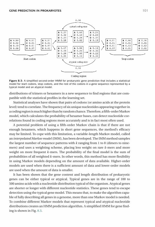
P1: JZP0521840988c08 CB1022/Xiong 0 521 84098 8 January 10, 2006 10:51
GENE PREDICTION IN PROKARYOTES 101
Figure 8.3: A simplified second-order HMM for prokaryotic gene prediction that includes a statisticalmodel for start codons, stop codons, and the rest of the codons in a gene sequence represented by atypical model and an atypical model.
distributions of trimers or hexamers in a new sequence to find regions that are com-patible with the statistical profiles in the learning set.
Statistical analyses have shown that pairs of codons (or amino acids at the proteinlevel) tend to correlate. The frequency of six unique nucleotides appearing together ina coding region is much higher than by random chance. Therefore, a fifth-order Markovmodel, which calculates the probability of hexamer bases, can detect nucleotide cor-relations found in coding regions more accurately and is in fact most often used.
A potential problem of using a fifth-order Markov chain is that if there are notenough hexamers, which happens in short gene sequences, the method’s efficacymay be limited. To cope with this limitation, a variable-length Markov model, calledan interpolated Markov model (IMM), has been developed. The IMM method samplesthe largest number of sequence patterns with k ranging from 1 to 8 (dimers to nine-mers) and uses a weighting scheme, placing less weight on rare k-mers and moreweight on more frequent k-mers. The probability of the final model is the sum ofprobabilities of all weighted k-mers. In other words, this method has more flexibilityin using Markov models depending on the amount of data available. Higher-ordermodels are used when there is a sufficient amount of data and lower-order modelsare used when the amount of data is smaller.
It has been shown that the gene content and length distribution of prokaryoticgenes can be either typical or atypical. Typical genes are in the range of 100 to500 amino acids with a nucleotide distribution typical of the organism. Atypical genesare shorter or longer with different nucleotide statistics. These genes tend to escapedetection using the typical gene model. This means that, to make the algorithm capa-ble of fully describing all genes in a genome, more than one Markov model is needed.To combine different Markov models that represent typical and atypical nucleotidedistributions creates an HMM prediction algorithm. A simplified HMM for gene find-ing is shown in Fig. 8.3.
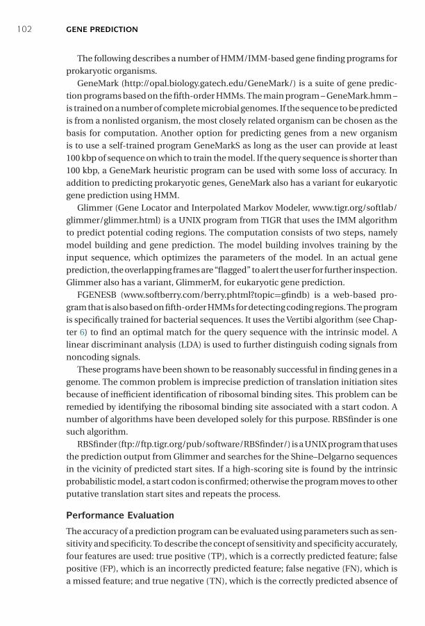
P1: JZP0521840988c08 CB1022/Xiong 0 521 84098 8 January 10, 2006 10:51
102 GENE PREDICTION
The following describes a number of HMM/IMM-based gene finding programs forprokaryotic organisms.
GeneMark (http://opal.biology.gatech.edu/GeneMark/) is a suite of gene predic-tion programs based on the fifth-order HMMs. The main program – GeneMark.hmm –is trained on a number of complete microbial genomes. If the sequence to be predictedis from a nonlisted organism, the most closely related organism can be chosen as thebasis for computation. Another option for predicting genes from a new organismis to use a self-trained program GeneMarkS as long as the user can provide at least100 kbp of sequence on which to train the model. If the query sequence is shorter than100 kbp, a GeneMark heuristic program can be used with some loss of accuracy. Inaddition to predicting prokaryotic genes, GeneMark also has a variant for eukaryoticgene prediction using HMM.
Glimmer (Gene Locator and Interpolated Markov Modeler, www.tigr.org/softlab/glimmer/glimmer.html) is a UNIX program from TIGR that uses the IMM algorithmto predict potential coding regions. The computation consists of two steps, namelymodel building and gene prediction. The model building involves training by theinput sequence, which optimizes the parameters of the model. In an actual geneprediction, the overlapping frames are “flagged” to alert the user for further inspection.Glimmer also has a variant, GlimmerM, for eukaryotic gene prediction.
FGENESB (www.softberry.com/berry.phtml?topic=gfindb) is a web-based pro-gram that is also based on fifth-order HMMs for detecting coding regions. The programis specifically trained for bacterial sequences. It uses the Vertibi algorithm (see Chap-ter 6) to find an optimal match for the query sequence with the intrinsic model. Alinear discriminant analysis (LDA) is used to further distinguish coding signals fromnoncoding signals.
These programs have been shown to be reasonably successful in finding genes in agenome. The common problem is imprecise prediction of translation initiation sitesbecause of inefficient identification of ribosomal binding sites. This problem can beremedied by identifying the ribosomal binding site associated with a start codon. Anumber of algorithms have been developed solely for this purpose. RBSfinder is onesuch algorithm.
RBSfinder (ftp://ftp.tigr.org/pub/software/RBSfinder/) is a UNIX program that usesthe prediction output from Glimmer and searches for the Shine–Delgarno sequencesin the vicinity of predicted start sites. If a high-scoring site is found by the intrinsicprobabilistic model, a start codon is confirmed; otherwise the program moves to otherputative translation start sites and repeats the process.
Performance Evaluation
The accuracy of a prediction program can be evaluated using parameters such as sen-sitivity and specificity. To describe the concept of sensitivity and specificity accurately,four features are used: true positive (TP), which is a correctly predicted feature; falsepositive (FP), which is an incorrectly predicted feature; false negative (FN), which isa missed feature; and true negative (TN), which is the correctly predicted absence of
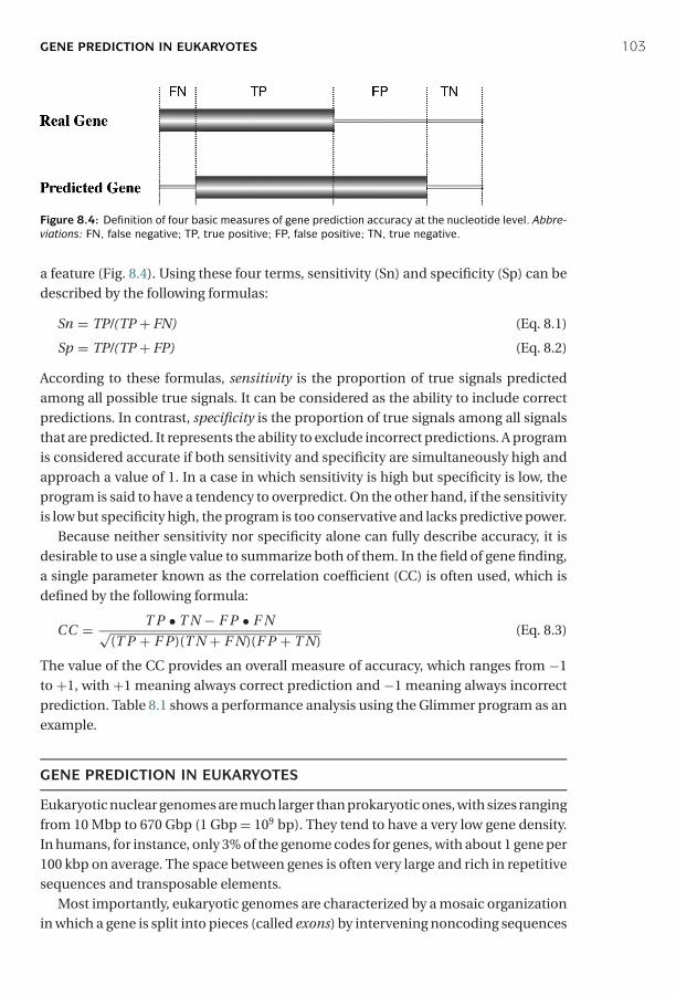
P1: JZP0521840988c08 CB1022/Xiong 0 521 84098 8 January 10, 2006 10:51
GENE PREDICTION IN EUKARYOTES 103
Figure 8.4: Definition of four basic measures of gene prediction accuracy at the nucleotide level. Abbre-viations: FN, false negative; TP, true positive; FP, false positive; TN, true negative.
a feature (Fig. 8.4). Using these four terms, sensitivity (Sn) and specificity (Sp) can bedescribed by the following formulas:
Sn = TP/(TP + FN) (Eq. 8.1)
Sp = TP/(TP + FP) (Eq. 8.2)
According to these formulas, sensitivity is the proportion of true signals predictedamong all possible true signals. It can be considered as the ability to include correctpredictions. In contrast, specificity is the proportion of true signals among all signalsthat are predicted. It represents the ability to exclude incorrect predictions. A programis considered accurate if both sensitivity and specificity are simultaneously high andapproach a value of 1. In a case in which sensitivity is high but specificity is low, theprogram is said to have a tendency to overpredict. On the other hand, if the sensitivityis low but specificity high, the program is too conservative and lacks predictive power.
Because neither sensitivity nor specificity alone can fully describe accuracy, it isdesirable to use a single value to summarize both of them. In the field of gene finding,a single parameter known as the correlation coefficient (CC) is often used, which isdefined by the following formula:
CC = T P • T N − F P • F N√(T P + F P)(T N + F N)(F P + T N)
(Eq. 8.3)
The value of the CC provides an overall measure of accuracy, which ranges from −1to +1, with +1 meaning always correct prediction and −1 meaning always incorrectprediction. Table 8.1 shows a performance analysis using the Glimmer program as anexample.
GENE PREDICTION IN EUKARYOTES
Eukaryotic nuclear genomes are much larger than prokaryotic ones, with sizes rangingfrom 10 Mbp to 670 Gbp (1 Gbp = 109 bp). They tend to have a very low gene density.In humans, for instance, only 3% of the genome codes for genes, with about 1 gene per100 kbp on average. The space between genes is often very large and rich in repetitivesequences and transposable elements.
Most importantly, eukaryotic genomes are characterized by a mosaic organizationin which a gene is split into pieces (called exons) by intervening noncoding sequences

P1: JZP0521840988c08 CB1022/Xiong 0 521 84098 8 January 10, 2006 10:51
104 GENE PREDICTION
TABLE 8.1. Performance Analysis of the Glimmer Program for Gene Predictionof Three Genomes
Species GC (%) FN FP Sensitivity Specificity
Campylobacter jejuni 30.5 10 19 99.3 98.7Haemophilus influenzae 38.2 3 54 99.8 96.1Helicobacter pylori 38.9 6 39 99.5 97.2
Note: The data sets were from three bacterial genomes (Aggarwal and Ramaswamy, 2002).Abbreviations: FN, false negative; FP, false positive.
(called introns) (Fig. 8.5). The nascent transcript from a eukaryotic gene is modi-fied in three different ways before becoming a mature mRNA for protein translation.The first is capping at the 5′ end of the transcript, which involves methylation atthe initial residue of the RNA. The second event is splicing, which is the process ofremoving introns and joining exons. The molecular basis of splicing is still not com-pletely understood. What is known currently is that the splicing process involves alarge RNA-protein complex called spliceosome. The reaction requires intermolecu-lar interactions between a pair of nucleotides at each end of an intron and the RNAcomponent of the spliceosome. To make the matter even more complex, some eukary-otic genes can have their transcripts spliced and joined in different ways to generatemore than one transcript per gene. This is the phenomenon of alternative splicing. Asto be discussed in more detail in Chapter 16, alternative splicing is a major mecha-nism for generating functional diversity in eukaryotic cells. The third modification ispolyadenylation, which is the addition of a stretch of As (∼250) at the 3′ end of the RNA.
Figure 8.5: Structure of a typical eukaryotic RNA as primary transcript from genomic DNA and asmature RNA after posttranscriptional processing. Abbreviations: UTR, untranslated region; poly-A,polyadenylation.
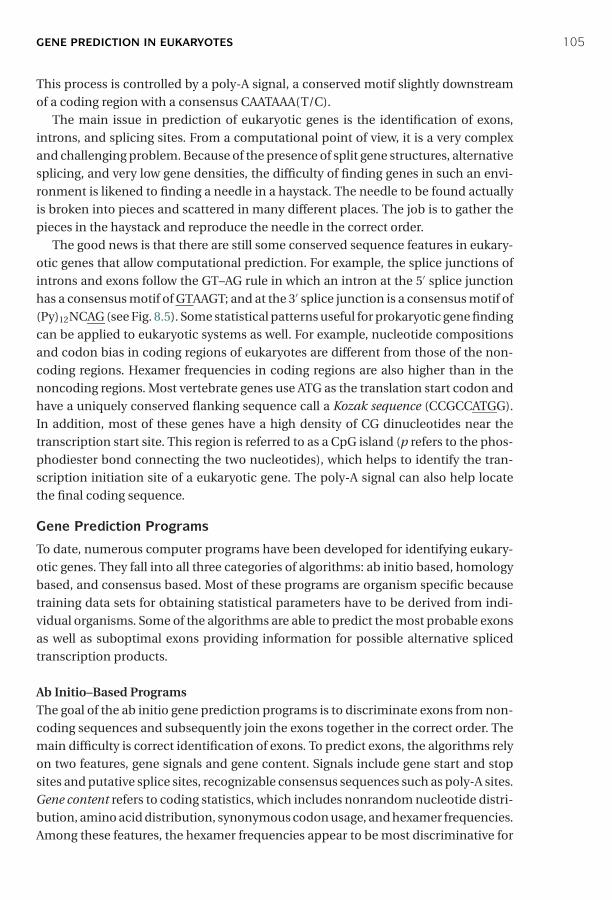
P1: JZP0521840988c08 CB1022/Xiong 0 521 84098 8 January 10, 2006 10:51
GENE PREDICTION IN EUKARYOTES 105
This process is controlled by a poly-A signal, a conserved motif slightly downstreamof a coding region with a consensus CAATAAA(T/C).
The main issue in prediction of eukaryotic genes is the identification of exons,introns, and splicing sites. From a computational point of view, it is a very complexand challenging problem. Because of the presence of split gene structures, alternativesplicing, and very low gene densities, the difficulty of finding genes in such an envi-ronment is likened to finding a needle in a haystack. The needle to be found actuallyis broken into pieces and scattered in many different places. The job is to gather thepieces in the haystack and reproduce the needle in the correct order.
The good news is that there are still some conserved sequence features in eukary-otic genes that allow computational prediction. For example, the splice junctions ofintrons and exons follow the GT–AG rule in which an intron at the 5′ splice junctionhas a consensus motif of GTAAGT; and at the 3′ splice junction is a consensus motif of(Py)12NCAG (see Fig. 8.5). Some statistical patterns useful for prokaryotic gene findingcan be applied to eukaryotic systems as well. For example, nucleotide compositionsand codon bias in coding regions of eukaryotes are different from those of the non-coding regions. Hexamer frequencies in coding regions are also higher than in thenoncoding regions. Most vertebrate genes use ATG as the translation start codon andhave a uniquely conserved flanking sequence call a Kozak sequence (CCGCCATGG).In addition, most of these genes have a high density of CG dinucleotides near thetranscription start site. This region is referred to as a CpG island (p refers to the phos-phodiester bond connecting the two nucleotides), which helps to identify the tran-scription initiation site of a eukaryotic gene. The poly-A signal can also help locatethe final coding sequence.
Gene Prediction Programs
To date, numerous computer programs have been developed for identifying eukary-otic genes. They fall into all three categories of algorithms: ab initio based, homologybased, and consensus based. Most of these programs are organism specific becausetraining data sets for obtaining statistical parameters have to be derived from indi-vidual organisms. Some of the algorithms are able to predict the most probable exonsas well as suboptimal exons providing information for possible alternative splicedtranscription products.
Ab Initio–Based ProgramsThe goal of the ab initio gene prediction programs is to discriminate exons from non-coding sequences and subsequently join the exons together in the correct order. Themain difficulty is correct identification of exons. To predict exons, the algorithms relyon two features, gene signals and gene content. Signals include gene start and stopsites and putative splice sites, recognizable consensus sequences such as poly-A sites.Gene content refers to coding statistics, which includes nonrandom nucleotide distri-bution, amino acid distribution, synonymous codon usage, and hexamer frequencies.Among these features, the hexamer frequencies appear to be most discriminative for
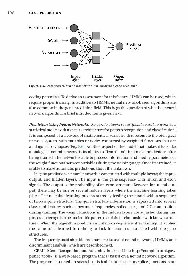
P1: JZP0521840988c08 CB1022/Xiong 0 521 84098 8 January 10, 2006 10:51
106 GENE PREDICTION
Figure 8.6: Architecture of a neural network for eukaryotic gene prediction.
coding potentials. To derive an assessment for this feature, HMMs can be used, whichrequire proper training. In addition to HMMs, neural network-based algorithms arealso common in the gene prediction field. This begs the question of what is a neuralnetwork algorithm. A brief introduction is given next.
Prediction Using Neural Networks. A neural network (or artificial neural network) is astatistical model with a special architecture for pattern recognition and classification.It is composed of a network of mathematical variables that resemble the biologicalnervous system, with variables or nodes connected by weighted functions that areanalogous to synapses (Fig. 8.6). Another aspect of the model that makes it look likea biological neural network is its ability to “learn” and then make predictions afterbeing trained. The network is able to process information and modify parameters ofthe weight functions between variables during the training stage. Once it is trained, itis able to make automatic predictions about the unknown.
In gene prediction, a neural network is constructed with multiple layers; the input,output, and hidden layers. The input is the gene sequence with intron and exonsignals. The output is the probability of an exon structure. Between input and out-put, there may be one or several hidden layers where the machine learning takesplace. The machine learning process starts by feeding the model with a sequenceof known gene structure. The gene structure information is separated into severalclasses of features such as hexamer frequencies, splice sites, and GC compositionduring training. The weight functions in the hidden layers are adjusted during thisprocess to recognize the nucleotide patterns and their relationship with known struc-tures. When the algorithm predicts an unknown sequence after training, it appliesthe same rules learned in training to look for patterns associated with the genestructures.
The frequently used ab initio programs make use of neural networks, HMMs, anddiscriminant analysis, which are described next.
GRAIL (Gene Recognition and Assembly Internet Link; http://compbio.ornl.gov/public/tools/) is a web-based program that is based on a neural network algorithm.The program is trained on several statistical features such as splice junctions, start
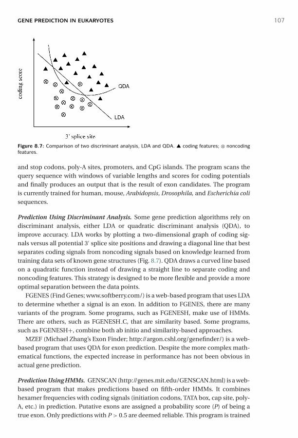
P1: JZP0521840988c08 CB1022/Xiong 0 521 84098 8 January 10, 2006 10:51
GENE PREDICTION IN EUKARYOTES 107
Figure 8.7: Comparison of two discriminant analysis, LDA and QDA. ▲ coding features; ⊗ noncodingfeatures.
and stop codons, poly-A sites, promoters, and CpG islands. The program scans thequery sequence with windows of variable lengths and scores for coding potentialsand finally produces an output that is the result of exon candidates. The programis currently trained for human, mouse, Arabidopsis, Drosophila, and Escherichia colisequences.
Prediction Using Discriminant Analysis. Some gene prediction algorithms rely ondiscriminant analysis, either LDA or quadratic discriminant analysis (QDA), toimprove accuracy. LDA works by plotting a two-dimensional graph of coding sig-nals versus all potential 3′ splice site positions and drawing a diagonal line that bestseparates coding signals from noncoding signals based on knowledge learned fromtraining data sets of known gene structures (Fig. 8.7). QDA draws a curved line basedon a quadratic function instead of drawing a straight line to separate coding andnoncoding features. This strategy is designed to be more flexible and provide a moreoptimal separation between the data points.
FGENES (Find Genes; www.softberry.com/) is a web-based program that uses LDAto determine whether a signal is an exon. In addition to FGENES, there are manyvariants of the program. Some programs, such as FGENESH, make use of HMMs.There are others, such as FGENESH C, that are similarity based. Some programs,such as FGENESH+, combine both ab initio and similarity-based approaches.
MZEF (Michael Zhang’s Exon Finder; http://argon.cshl.org/genefinder/) is a web-based program that uses QDA for exon prediction. Despite the more complex math-ematical functions, the expected increase in performance has not been obvious inactual gene prediction.
Prediction Using HMMs. GENSCAN (http://genes.mit.edu/GENSCAN.html) is a web-based program that makes predictions based on fifth-order HMMs. It combineshexamer frequencies with coding signals (initiation codons, TATA box, cap site, poly-A, etc.) in prediction. Putative exons are assigned a probability score (P) of being atrue exon. Only predictions with P > 0.5 are deemed reliable. This program is trained

P1: JZP0521840988c08 CB1022/Xiong 0 521 84098 8 January 10, 2006 10:51
108 GENE PREDICTION
for sequences from vertebrates, Arabidopsis, and maize. It has been used extensivelyin annotating the human genome (see Chapter 17).
HMMgene (www.cbs.dtu.dk/services/HMMgene) is also an HMM-based web pro-gram. The unique feature of the program is that it uses a criterion called the conditionalmaximum likelihood to discriminate coding from noncoding features. If a sequencealready has a subregion identified as coding region, which may be based on similaritywith cDNAs or proteins in a database, these regions are locked as coding regions. AnHMM prediction is subsequently made with a bias toward the locked region and isextended from the locked region to predict the rest of the gene coding regions andeven neighboring genes. The program is in a way a hybrid algorithm that uses bothab initio-based and homology-based criteria.
Homology-Based ProgramsHomology-based programs are based on the fact that exon structures and exonsequences of related species are highly conserved. When potential coding frames in aquery sequence are translated and used to align with closest protein homologs foundin databases, near perfectly matched regions can be used to reveal the exon bound-aries in the query. This approach assumes that the database sequences are correct.It is a reasonable assumption in light of the fact that many homologous sequencesto be compared with are derived from cDNA or expressed sequence tags (ESTs) ofthe same species. With the support of experimental evidence, this method becomesrather efficient in finding genes in an unknown genomic DNA.
The drawback of this approach is its reliance on the presence of homologs indatabases. If the homologs are not available in the database, the method cannotbe used. Novel genes in a new species cannot be discovered without matches in thedatabase. A number of publicly available programs that use this approach are dis-cussed next.
GenomeScan (http://genes.mit.edu/genomescan.html) is a web-based server thatcombines GENSCAN prediction results with BLASTX similarity searches. The userprovides genomic DNA and protein sequences from related species. The genomicDNA is translated in all six frames to cover all possible exons. The translated exonsare then used to compare with the user-supplied protein sequences. Translatedgenomic regions having high similarity at the protein level receive higher scores.The same sequence is also predicted with a GENSCAN algorithm, which gives exonsprobability scores. Final exons are assigned based on combined score informationfrom both analyses.
EST2Genome (http://bioweb.pasteur.fr/seqanal/interfaces/est2genome.html) is aweb-based program purely based on the sequence alignment approach to defineintron–exon boundaries. The program compares an EST (or cDNA) sequence with agenomic DNA sequence containing the corresponding gene. The alignment is doneusing a dynamic programming–based algorithm. One advantage of the approach isthe ability to find very small exons and alternatively spliced exons that are very difficultto predict by any ab initio–type algorithms. Another advantage is that there is no need
P1: JZP0521840988c08 CB1022/Xiong 0 521 84098 8 January 10, 2006 10:51
GENE PREDICTION IN EUKARYOTES 109
for model training, which provides much more flexibility for gene prediction. Thelimitation is that EST or cDNA sequences often contain errors or even introns if thetranscripts are not completely spliced before reverse transcription.
SGP-1 (Syntenic Gene Prediction; http://195.37.47.237/sgp-1/) is a similarity-basedweb program that aligns two genomic DNA sequences from closely related organ-isms. The program translates all potential exons in each sequence and does pair-wise alignment for the translated protein sequences using a dynamic programmingapproach. The near-perfect matches at the protein level define coding regions. Simi-lar to EST2Genome, there is no training needed. The limitation is the need for twohomologous sequences having similar genes with similar exon structures; if this con-dition is not met, a gene escapes detection from one sequence when there is nocounterpart in another sequence.
TwinScan (http://genes.cs.wustl.edu/) is also a similarity-based gene-findingserver. It is similar to GenomeScan in that it uses GenScan to predict all possibleexons from the genomic sequence. The putative exons are used for BLAST searchingto find closest homologs. The putative exons and homologs from BLAST searching arealigned to identify the best match. Only the closest match from a genome database isused as a template for refining the previous exon selection and exon boundaries.
Consensus-Based ProgramsBecause different prediction programs have different levels of sensitivity and speci-ficity, it makes sense to combine results of multiple programs based on consensus.This idea has prompted development of consensus-based algorithms. These pro-grams work by retaining common predictions agreed by most programs and removinginconsistent predictions. Such an integrated approach may improve the specificity bycorrecting the false positives and the problem of overprediction. However, since thisprocedure punishes novel predictions, it may lead to lowered sensitivity and missedpredictions. Two examples of consensus-based programs are given next.
GeneComber (www.bioinformatics.ubc.ca/genecomber/index.php) is a webserver that combines HMMgene and GenScan prediction results. The consistencyof both prediction methods is calculated. If the two predictions match, the exon scoreis reinforced. If not, exons are proposed based on separate threshold scores.
DIGIT (http://digit.gsc.riken.go.jp/cgi-bin/index.cgi) is another consensus-basedweb server. It uses prediction from three ab initio programs – FGENESH, GENSCAN,and HMMgene. It first compiles all putative exons from the three gene-finders andassigns ORFs with associated scores. It then searches a set of exons with the highestadditive score under the reading frame constraints. During this process, a Bayesianprocedure and HMMs are used to infer scores and search the optimal exon set whichgives the final designation of gene structure.
Performance EvaluationBecause of extra layers of complexity for eukaryotic gene prediction, the sensitivityand specificity have to be defined on the levels of nucleotides, exons, and entire genes.
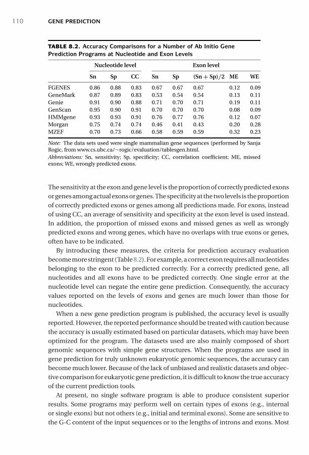
P1: JZP0521840988c08 CB1022/Xiong 0 521 84098 8 January 10, 2006 10:51
110 GENE PREDICTION
TABLE 8.2. Accuracy Comparisons for a Number of Ab Initio GenePrediction Programs at Nucleotide and Exon Levels
Nucleotide level Exon level
Sn Sp CC Sn Sp (Sn + Sp)/2 ME WE
FGENES 0.86 0.88 0.83 0.67 0.67 0.67 0.12 0.09GeneMark 0.87 0.89 0.83 0.53 0.54 0.54 0.13 0.11Genie 0.91 0.90 0.88 0.71 0.70 0.71 0.19 0.11GenScan 0.95 0.90 0.91 0.70 0.70 0.70 0.08 0.09HMMgene 0.93 0.93 0.91 0.76 0.77 0.76 0.12 0.07Morgan 0.75 0.74 0.74 0.46 0.41 0.43 0.20 0.28MZEF 0.70 0.73 0.66 0.58 0.59 0.59 0.32 0.23
Note: The data sets used were single mammalian gene sequences (performed by SanjaRogic, from www.cs.ubc.ca/∼rogic/evaluation/tablesgen.html.Abbreviations: Sn, sensitivity; Sp, specificity; CC, correlation coefficient; ME, missedexons; WE, wrongly predicted exons.
The sensitivity at the exon and gene level is the proportion of correctly predicted exonsor genes among actual exons or genes. The specificity at the two levels is the proportionof correctly predicted exons or genes among all predictions made. For exons, insteadof using CC, an average of sensitivity and specificity at the exon level is used instead.In addition, the proportion of missed exons and missed genes as well as wronglypredicted exons and wrong genes, which have no overlaps with true exons or genes,often have to be indicated.
By introducing these measures, the criteria for prediction accuracy evaluationbecome more stringent (Table 8.2). For example, a correct exon requires all nucleotidesbelonging to the exon to be predicted correctly. For a correctly predicted gene, allnucleotides and all exons have to be predicted correctly. One single error at thenucleotide level can negate the entire gene prediction. Consequently, the accuracyvalues reported on the levels of exons and genes are much lower than those fornucleotides.
When a new gene prediction program is published, the accuracy level is usuallyreported. However, the reported performance should be treated with caution becausethe accuracy is usually estimated based on particular datasets, which may have beenoptimized for the program. The datasets used are also mainly composed of shortgenomic sequences with simple gene structures. When the programs are used ingene prediction for truly unknown eukaryotic genomic sequences, the accuracy canbecome much lower. Because of the lack of unbiased and realistic datasets and objec-tive comparison for eukaryotic gene prediction, it is difficult to know the true accuracyof the current prediction tools.
At present, no single software program is able to produce consistent superiorresults. Some programs may perform well on certain types of exons (e.g., internalor single exons) but not others (e.g., initial and terminal exons). Some are sensitive tothe G-C content of the input sequences or to the lengths of introns and exons. Most
P1: JZP0521840988c08 CB1022/Xiong 0 521 84098 8 January 10, 2006 10:51
FURTHER READING 111
programs make overpredictions when genes contain long introns. In sum, they allsuffer from the problem of generating a high number of false positives and false nega-tives. This is especially true for ab initio–based algorithms. For complex genomes suchas the human genome, most popular programs can predict no more than 40% of thegenes exactly right. Drawing consensus from results by multiple prediction programsmay enhance performance to some extent.
SUMMARY
Computational prediction of genes is one of the most important steps of genomesequence analysis. For prokaryotic genomes, which are characterized by high genedensity and noninterrupted genes, prediction of genes is easier than for eukaryoticgenomes. Current prokaryotic gene prediction algorithms, which are based on HMMs,have achieved reasonably good accuracy. Many difficulties still persist for eukaryoticgene prediction. The difficulty mainly results from the low gene density and splitgene structure of eukaryotic genomes. Current algorithms are either ab initio based,homology based, or a combination of both. For ab initio–based eukaryotic gene pre-diction, the HMM type of algorithm has overall better performance in differentiatingintron–exon boundaries. The major limitation is the dependency on training of thestatistical models, which renders the method to be organism specific. The homology-based algorithms in combination with HMMs may yield improved accuracy. Themethod is limited by the availability of identifiable sequence homologs in databases.The combined approach that integrates statistical and homology information maygenerate further improved performance by detecting more genes and more exonscorrectly. With rapid advances in computational techniques and understanding of thesplicing mechanism, it is hoped that reliable eukaryotic gene prediction can becomemore feasible in the near future.
FURTHER READING
Aggarwal, G., and Ramaswamy, R. 2002. Ab initio gene identification: Prokaryote genome anno-tation with GeneScan and GLIMMER. J. Biosci. 27:7–14.
Ashurst, J. L., and Collins, J. E. 2003. Gene annotation: Prediction and testing. Annu. Rev.Genomics Hum. Genet. 4:69–88.
Azad, R. K., and Borodovsky, M. 2004. Probabilistic methods of identifying genes in prokaryoticgenomes: Connections to the HMM theory. Brief. Bioinform. 5:118–30.
Cruveiller, S., Jabbari, K., Clay, O., and Bemardi, G. 2003. Compositional features of eukaryoticgenomes for checking predicted genes. Brief. Bioinform. 4:43–52.
Davuluri, R. V., and Zhang, M. Q. 2003. “Computer software to find genes in plant genomic DNA.”In Plant Functional Genomics, edited by E. Grotewold, 87–108. Totowa, NJ: Human Press.
Guigo, R., and Wiehe, T. 2003. “Gene prediction accuracy in large DNA sequences.” In Frontiersin Computational Genomics, edited by M. Y. Galperin and E. V. Koonin, 1–33. Norfolk, UK:Caister Academic Press.

P1: JZP0521840988c08 CB1022/Xiong 0 521 84098 8 January 10, 2006 10:51
112 GENE PREDICTION
Guigo, R., Dermitzakis, E. T., Agarwal, P., Ponting, C. P., Parra, G., Reymond, A., Abril, J. F., et alR. 2003. Comparison of mouse and human genomes followed by experimental verificationyields an estimated 1,019 additional genes. Proc. Natl. Acad. Sci. USA 100:1140–5.
Li, W., and Godzik, A. 2002. Discovering new genes with advanced homology detection. TrendsBiotechnol. 20:315–16.
Makarov, V. 2002. Computer programs for eukaryotic gene prediction. Brief. Bioinform. 3:195–9.Mathe, C., Sagot, M. F., Schiex, T., and Rouze, P. 2002. Current methods of gene prediction, their
strengths and weaknesses. Nucleic Acids Res. 30:4103–17.Parra, G., Agarwal, P., Abril, J. F., Wiehe, T., Fickett, J. W., and Guigo, R. 2003. Comparative gene
prediction in human and mouse. Genome Res. 13:108–17.Wang, J., Li, S., Zhang, Y., Zheng, H., Xu, Z., Ye, J., Yu, J., and Wong, G. K. 2003. Vertebrate gene
predictions and the problem of large genes. Nat. Rev. Genet. 4:741–9.Wang, Z., Chen, Y., and Li, Y. 2004. A brief review of computational gene prediction methods.
Geno. Prot. Bioinfo. 4:216–21.Zhang, M. Q. 2002. Computational prediction of eukaryotic protein coding genes. Nat. Rev.
Genetics. 3:698–709.
P1: JZP0521840988c09 CB1022/Xiong 0 521 84098 8 January 10, 2006 10:56
CHAPTER NINE
Promoter and Regulatory Element Prediction
An issue related to gene prediction is promoter prediction. Promoters are DNA ele-ments located in the vicinity of gene start sites (which should not be confused with thetranslation start sites) and serve as binding sites for the gene transcription machinery,consisting of RNA polymerases and transcription factors. Therefore, these DNA ele-ments directly regulate gene expression. Promoters and regulatory elements are tradi-tionally determined by experimental analysis. The process is extremely time consum-ing and laborious. Computational prediction of promoters and regulatory elementsis especially promising because it has the potential to replace a great deal of extensiveexperimental analysis.
However, computational identification of promoters and regulatory elements isalso a very difficult task, for several reasons. First, promoters and regulatory elementsare not clearly defined and are highly diverse. Each gene seems to have a unique com-bination of sets of regulatory motifs that determine its unique temporal and spatialexpression. There is currently a lack of sufficient understanding of all the necessaryregulatory elements for transcription. Second, the promoters and regulatory elementscannot be translated into protein sequences to increase the sensitivity for their detec-tion. Third, promoter and regulatory sites to be predicted are normally short (six toeight nucleotides) and can be found in essentially any sequence by random chance,thus resulting in high rates of false positives associated with theoretical predictions.
Current solutions for providing preliminary identification of these elements are tocombine a multitude of features and use sophisticated algorithms that give either abinitio–based predictions or predictions based on evolutionary information or experi-mental data. These computational approaches are described in detail in this chapterfollowing a brief introduction to the structures of promoters and regulatory elementsin both prokaryotes and eukaryotes.
PROMOTER AND REGULATORY ELEMENTS IN PROKARYOTES
In bacteria, transcription is initiated by RNA polymerase, which is a multi-subunitenzyme. The σ subunit (e.g., σ 70) of the RNA polymerase is the protein that recognizesspecific sequences upstream of a gene and allows the rest of the enzyme complexto bind. The upstream sequence where the σ protein binds constitutes the promotersequence. This includes the sequence segments located 35 and 10 base pairs(bp) upstream from the transcription start site. They are also referred to as the−35 and −10 boxes. For the σ 70 subunit in Escherichia coli, for example, the −35 box
113
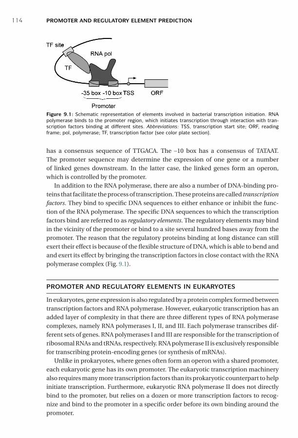
P1: JZP0521840988c09 CB1022/Xiong 0 521 84098 8 January 10, 2006 10:56
114 PROMOTER AND REGULATORY ELEMENT PREDICTION
Figure 9.1: Schematic representation of elements involved in bacterial transcription initiation. RNApolymerase binds to the promoter region, which initiates transcription through interaction with tran-scription factors binding at different sites. Abbreviations: TSS, transcription start site; ORF, readingframe; pol, polymerase; TF, transcription factor (see color plate section).
has a consensus sequence of TTGACA. The –10 box has a consensus of TATAAT.The promoter sequence may determine the expression of one gene or a numberof linked genes downstream. In the latter case, the linked genes form an operon,which is controlled by the promoter.
In addition to the RNA polymerase, there are also a number of DNA-binding pro-teins that facilitate the process of transcription. These proteins are called transcriptionfactors. They bind to specific DNA sequences to either enhance or inhibit the func-tion of the RNA polymerase. The specific DNA sequences to which the transcriptionfactors bind are referred to as regulatory elements. The regulatory elements may bindin the vicinity of the promoter or bind to a site several hundred bases away from thepromoter. The reason that the regulatory proteins binding at long distance can stillexert their effect is because of the flexible structure of DNA, which is able to bend andand exert its effect by bringing the transcription factors in close contact with the RNApolymerase complex (Fig. 9.1).
PROMOTER AND REGULATORY ELEMENTS IN EUKARYOTES
In eukaryotes, gene expression is also regulated by a protein complex formed betweentranscription factors and RNA polymerase. However, eukaryotic transcription has anadded layer of complexity in that there are three different types of RNA polymerasecomplexes, namely RNA polymerases I, II, and III. Each polymerase transcribes dif-ferent sets of genes. RNA polymerases I and III are responsible for the transcription ofribosomal RNAs and tRNAs, respectively. RNA polymerase II is exclusively responsiblefor transcribing protein-encoding genes (or synthesis of mRNAs).
Unlike in prokaryotes, where genes often form an operon with a shared promoter,each eukaryotic gene has its own promoter. The eukaryotic transcription machineryalso requires many more transcription factors than its prokaryotic counterpart to helpinitiate transcription. Furthermore, eukaryotic RNA polymerase II does not directlybind to the promoter, but relies on a dozen or more transcription factors to recog-nize and bind to the promoter in a specific order before its own binding around thepromoter.
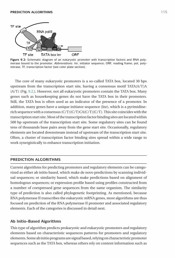
P1: JZP0521840988c09 CB1022/Xiong 0 521 84098 8 January 10, 2006 10:56
PREDICTION ALGORITHMS 115
Figure 9.2: Schematic diagram of an eukaryotic promoter with transcription factors and RNA poly-merase bound to the promoter. Abbreviations: Inr, initiator sequence; ORF, reading frame; pol, poly-merase; TF, transcription factor (see color plate section).
The core of many eukaryotic promoters is a so-called TATA box, located 30 bpsupstream from the transcription start site, having a consensus motif TATA(A/T)A(A/T) (Fig. 9.2.). However, not all eukaryotic promoters contain the TATA box. Manygenes such as housekeeping genes do not have the TATA box in their promoters.Still, the TATA box is often used as an indicator of the presence of a promoter. Inaddition, many genes have a unique initiator sequence (Inr), which is a pyrimidine-rich sequence with a consensus (C/T)(C/T)CA(C/T)(C/T). This site coincides with thetranscription start site. Most of the transcription factor binding sites are located within500 bp upstream of the transcription start site. Some regulatory sites can be foundtens of thousands base pairs away from the gene start site. Occasionally, regulatoryelements are located downstream instead of upstream of the transcription start site.Often, a cluster of transcription factor binding sites spread within a wide range towork synergistically to enhance transcription initiation.
PREDICTION ALGORITHMS
Current algorithms for predicting promoters and regulatory elements can be catego-rized as either ab initio based, which make de novo predictions by scanning individ-ual sequences; or similarity based, which make predictions based on alignment ofhomologous sequences; or expression profile based using profiles constructed froma number of coexpressed gene sequences from the same organism. The similaritytype of prediction is also called phylogenetic footprinting. As mentioned, becauseRNA polymerase II transcribes the eukaryotic mRNA genes, most algorithms are thusfocused on prediction of the RNA polymerase II promoter and associated regulatoryelements. Each of the categories is discussed in detail next.
Ab Initio–Based Algorithms
This type of algorithm predicts prokaryotic and eukaryotic promoters and regulatoryelements based on characteristic sequences patterns for promoters and regulatoryelements. Some ab initio programs are signal based, relying on characteristic promotersequences such as the TATA box, whereas others rely on content information such as

P1: JZP0521840988c09 CB1022/Xiong 0 521 84098 8 January 10, 2006 10:56
116 PROMOTER AND REGULATORY ELEMENT PREDICTION
hexamer frequencies. The advantage of the ab initio method is that the sequence canbe applied as such without having to obtain experimental information. The limitationis the need for training, which makes the prediction programs species specific. Inaddition, this type of method has a difficulty in discovering new, unknown motifs.
The conventional approach to detecting a promoter or regulatory site is throughmatching a consensus sequence pattern represented by regular expressions (seeChapter 7) or matching a position-specific scoring matrix (PSSM; see Chapter 6)constructed from well-characterized binding sites. In either case, the consensussequences or the matrices are relatively short, covering 6 to 10 bases. As describedin Chapter 7, to determine whether a query sequence matches a weight matrix, thesequence is scanned through the matrix. Scores of matches and mismatches at allmatrix positions are summed up to give a log odds score, which is then evaluated forstatistical significance. This simple approach, however, often has difficulty differen-tiating true promoters from random sequence matches and generates high rates offalse positives as a result.
To better discriminate true motifs from background noise, a new generation ofalgorithms has been developed that take into account the higher order correlation ofmultiple subtle features by using discriminant functions, neural networks, or hiddenMarkov models (HMMs) that are capable of incorporating more neighboring sequenceinformation. To further improve the specificity of prediction, some algorithms selec-tively exclude coding regions and focus on the upstream regions (0.5 to 2.0 kb) only,which are most likely to contain promoters. In that sense, promoter prediction andgene prediction are coupled.
Prediction for ProkaryotesOne of the unique aspects in prokaryotic promoter prediction is the determinationof operon structures, because genes within an operon share a common promoterlocated upstream of the first gene of the operon. Thus, operon prediction is the keyin prokaryotic promoter prediction. Once an operon structure is known, only the firstgene is predicted for the presence of a promoter and regulatory elements, whereasother genes in the operon do not possess such DNA elements.
There are a number of methods available for prokaryotic operon prediction. Themost accurate is a set of simple rules developed by Wang et al. (2004). This methodrelies on two kinds of information: gene orientation and intergenic distances of a pairof genes of interest and conserved linkage of the genes based on comparative genomicanalysis. More about gene linkage patterns across genomes is introduced in Chapters16 and 18. A scoring scheme is developed to assign operons with different levels ofconfidence (Fig. 9.3). This method is claimed to produce accurate identification of anoperon structure, which in turn facilitates the promoter prediction.
This newly developed scoring approach is, however, not yet available as a computerprogram. The prediction can be done manually using the rules, however. The fewdedicated programs for prokaryotic promoter prediction do not apply the Wang et al.rule for historical reasons. The most frequently used program is BPROM.

P1: JZP0521840988c09 CB1022/Xiong 0 521 84098 8 January 10, 2006 10:56
PREDICTION ALGORITHMS 117
Figure 9.3: Prediction of operons in prokaryotes based on a scoring scheme developed by Wang et al.(2004). This method states that, for two adjacent genes transcribed in the same orientation and withouta ρ-independent transcription termination signal in between, the score is assigned 0 if the intergenic dis-tance is larger than 300 bp regardless of the gene linkage pattern or if the distance is larger than 100 bpwith the linkage not observed in other genomes. The score is assigned 1 if the intergenic distance islarger than 60 bp with the linkage shared in less than five genomes. The score is assigned 2 if thedistance of the two genes is between 30 and 60 bp with the linkage shared in less than five genomesor if the distance is between 50 and 300 bp with the linkage shared in between five to ten genomes.The score is assigned 3 if the intergenic distance is less than 30 bp regardless of the conserved linkagepattern or if the linkage is conserved in more than ten genomes regardless of the intergenic distance orif the distance is less than 50 bp with the linkage shared in between five to ten genomes. A minimumscore of 2 is considered the threshold for assigning the two genes in one operon.
BPROM (www.softberry.com/berry.phtml?topic=bprom&group=programs &sub-group=gfindb) is a web-based program for prediction of bacterial promoters. It usesa linear discriminant function (see Chapter 8) combined with signal and contentinformation such as consensus promoter sequence and oligonucleotide compositionof the promoter sites. This program first predicts a given sequence for bacterial operonstructures by using an intergenic distance of 100 bp as basis for distinguishing genesto be in an operon. This rule is more arbitrary than the Wang et al. rule, leading to highrates of false positives. Once the operons are assigned, the program is able to predictputative promoter sequences. Because most bacterial promoters are located within200 bp of the protein coding region, the program is most effectively used when about
P1: JZP0521840988c09 CB1022/Xiong 0 521 84098 8 January 10, 2006 10:56
118 PROMOTER AND REGULATORY ELEMENT PREDICTION
200 bp of upstream sequence of the first gene of an operon is supplied as input toincrease specificity.
FindTerm (http://sun1.softberry.com/berry.phtml?topic=findterm&group=programs&subgroup=gfindb) is a program for searching bacterial ρ-independenttermination signals located at the end of operons. It is available from the same siteas FGENES and BPROM. The predictions are made based on matching of knownprofiles of the termination signals combined with energy calculations for the derivedRNA secondary structures for the putative hairpin-loop structure (see Chapter 16).The sequence region that scores best in features and energy terms is chosen as theprediction. The information can sometimes be useful in defining an operon.
Prediction for EukaryotesThe ab initio method for predicting eukaryotic promoters and regulatory elementsalso relies on searching the input sequences for matching of consensus patternsof known promoters and regulatory elements. The consensus patterns are derivedfrom experimentally determined DNA binding sites which are compiled into pro-files and stored in a database for scanning an unknown sequence to find simi-lar conserved patterns. However, this approach tends to generate very high rateof false positives owing to nonspecific matches with the short sequence patterns.Furthermore, because of the high variability of transcription factor binding sites,the simple sequence matching often misses true promoter sites, creating falsenegatives.
To increase the specificity of prediction, a unique feature of eukaryotic promoteris employed, which is the presence of CpG islands. It is known that many vertebrategenes are characterized by a high density of CG dinucleotides near the promoterregion overlapping the transcription start site (see Chapter 8). By identifying the CpGislands, promoters can be traced on the immediate upstream region from the islands.By combining CpG islands and other promoter signals, the accuracy of prediction canbe improved. Several programs have been developed based on the combined featuresto predict the transcription start sites in particular.
As discussed, the eukaryotic transcription initiation requires cooperation of a largenumber of transcription factors. Cooperativity means that the promoter regions tendto contain a high density of protein-binding sites. Thus, finding a cluster of transcrip-tion factor binding sites often enhances the probability of individual binding siteprediction.
A number of representatives of ab initio promoter prediction algorithms that incor-porate the unique properties of eukaryotic promoters are introduced next.
CpGProD (http://pbil.univ-lyon1.fr/software/cpgprod.html) is a web-based pro-gram that predicts promoters containing a high density of CpG islands in mam-malian genomic sequences. It calculates moving averages of GC% and CpG ratios(observed/expected) over a window of a certain size (usually 200 bp). When the val-ues are above a certain threshold, the region is identified as a CpG island.

P1: JZP0521840988c09 CB1022/Xiong 0 521 84098 8 January 10, 2006 10:56
PREDICTION ALGORITHMS 119
Eponine (http://servlet.sanger.ac.uk:8080/eponine/) is a web-based program thatpredicts transcription start sites based on a series of preconstructed PSSMs of severalregulatory sites, such as the TATA box, the CCAAT box, and CpG islands. The querysequence from a mammalian source is scanned through the PSSMs. The sequencestretches with high-score matching to all the PSSMs, as well as matching of the spacingbetween the elements, are declared transcription start sites. A Bayesian method is alsoused in decision making.
Cluster-Buster (http://zlab.bu.edu/cluster-buster/cbust.html) is an HMM-based,web-based program designed to find clusters of regulatory binding sites. It works bydetecting a region of high concentration of known transcription factor binding sitesand regulatory motifs. A query sequence is scanned with a window size of 1 kb forputative regulatory motifs using motif HMMs. If multiple motifs are detected within awindow, a positive score is assigned to each motif found. The total score of the windowis the sum of each motif score subtracting a gap penalty, which is proportional to thedistances between motifs. If the score of a certain region is above a certain threshold,it is predicted to contain a regulatory cluster.
FirstEF (First Exon Finder; http://rulai.cshl.org/tools/FirstEF/) is a web-based pro-gram that predicts promoters for human DNA. It integrates gene prediction with pro-moter prediction. It uses quadratic discriminant functions (see Chapter 8) to calculatethe probabilities of the first exon of a gene and its boundary sites. A segment of DNA(15 kb) upstream of the first exon is subsequently extracted for promoter predictionon the basis of scores for CpG islands.
McPromoter (http://genes.mit.edu/McPromoter.html) is a web-based programthat uses a neural network to make promoter predictions. It has a unique promotermodel containing six scoring segments. The program scans a window of 300 bases forthe likelihoods of being in each of the coding, noncoding, and promoter regions. Theinput for the neural network includes parameters for sequence physical properties,such as DNA bendability, plus signals such as the TATA box, initiator box, and CpGislands. The hidden layer combines all the features to derive an overall likelihood fora site being a promoter. Another unique feature is that McPromoter does not requirethat certain patterns must be present, but instead the combination of all features isimportant. For instance, even if the TATA box score is very low, a promoter predictioncan still be made if the other features score highly. The program is currently trainedfor Drosophila and human sequences.
TSSW (www.softberry.com/berry.phtml?topic=promoter) is a web program thatdistinguishes promoter sequences from non-promoter sequences based on a combi-nation of unique content information such as hexamer/trimer frequencies and sig-nal information such the TATA box in the promoter region. The values are fed to alinear discriminant function (see Chapter 8) to separate true motifs from backgroundnoise.
CONPRO (http://stl.bioinformatics.med.umich.edu/conpro) is a web-based pro-gram that uses a consensus method to identify promoter elements for human DNA.
P1: JZP0521840988c09 CB1022/Xiong 0 521 84098 8 January 10, 2006 10:56
120 PROMOTER AND REGULATORY ELEMENT PREDICTION
To use the program, a user supplies the transcript sequence of a gene (cDNA). Theprogram uses the information to search the human genome database for the positionof the gene. It then uses the GENSCAN program to predict 5′ untranslated exons in theupstream region. Once the 5′-most exon is located, a further upstream region (1.5 kb)is used for promoter prediction, which relies on a combination of five promoter pre-diction programs, TSSG, TSSW, NNPP, PROSCAN, and PromFD. For each program, thehighest score prediction is taken as the promoter in the region. If three predictionsfall within a 100-bp region, this is considered a consensus prediction. If no three-wayconsensus is achieved, TSSG and PromFD predictions are taken. Because no cod-ing sequence is used in prediction, specificity is improved relative to each individualprogram.
Phylogenetic Footprinting–Based Method
It has been observed that promoter and regulatory elements from closely relatedorganisms such as human and mouse are highly conserved. The conservation is bothat the sequence level and at the level of organization of the elements. Therefore, it ispossible to obtain such promoter sequences for a particular gene through compar-ative analysis. The identification of conserved noncoding DNA elements that servecrucial functional roles is referred to as phylogenetic footprinting; the elements arecalled phylogenetic footprints. This type of method can apply to both prokaryotic andeukaryotic sequences.
The selection of organisms for comparison is an important consideration in thistype of analysis. If the pair of organisms selected are too closely related, such ashuman and chimpanzee, the sequence difference between them may not be sufficientto filter out functional elements. On the other hand, if the organisms’ evolutionarydistances are too long, such as between human and fish, long evolutionary divergencemay render promoter and other elements undetectable. One example of appropriateselection of species is the use of human and mouse sequences, which often yieldsinformative results.
Another caveat of phylogenetic footprinting is to extract noncoding sequencesupstream of corresponding genes and focus the comparison to this region only, whichhelps to prevent false positives. The predictive value of this method also depends onthe quality of the subsequent sequence alignments. The advanced alignment pro-grams introduced in Chapter 5 can be used. Even more sophisticated expectationmaximization (EM) and Gibbs sampling algorithms can be used in detecting weaklyconserved motifs.
There are software programs specifically designed to take advantage of the pre-sence of phylogenetic footprints to make comparisons among a number of relatedspecies to identify putative transcription factor binding sites. The advantage in imple-menting the algorithms is that no training of the probabilistic models is required;hence, it is more broadly applicable. There is also a potential to discover new regulatory
P1: JZP0521840988c09 CB1022/Xiong 0 521 84098 8 January 10, 2006 10:56
PREDICTION ALGORITHMS 121
motifs shared among organisms. The obvious limitation is the constraint on the evo-lutionary distances among the orthologous sequences.
ConSite (http://mordor.cgb.ki.se/cgi-bin/CONSITE/consite) is a web server thatfinds putative promoter elements by comparing two orthologous sequences. Theuser provides two individual sequences which are aligned by ConSite using a globalalignment algorithm. Alternatively, the program accepts precomputed alignment.Conserved regions are identified by calculating identity scores, which are then usedto compare against a motif database of regulatory sites (TRANSFAC). High-scoringsequence segments upstream of genes are returned as putative regulatory elements.
rVISTA (http://rvista.dcode.org/) is a similar cross-species comparison tool forpromoter recognition. The program uses two orthologous sequences as input and firstidentifies all putative regulatory motifs based on TRANSFAC matches. It then alignsthe two sequences using a local alignment strategy. The motifs that have the highestpercent identity in the pairwise comparison are presented graphically as regulatoryelements.
PromH(W) (www.softberry.com/berry.phtml?topic=promhw&group=programs&subgroup=promoter) is a web-based program that predicts regulatory sites by pair-wise sequence comparison. The user supplies two orthologous sequences, which arealigned by the program to identify conserved regions. These regions are subsequentlypredicted for RNA polymerase II promoter motifs in both sequences using the TSSWprogram. Only the conserved regions having high scored promoter motifs are returnedas results.
Bayes aligner (www.bioinfo.rpi.edu/applications/bayesian/bayes/bayes align12.pl) is a web-based footprinting program. It aligns two sequences using a Bayesianalgorithm which is a unique sequence alignment method. Instead of returning a singlebest alignment, the method generates a distribution of a large number of alignmentsusing a full range of scoring matrices and gap penalties. Posterior probability values,which are considered estimates of the true alignment, are calculated for each align-ment. By studying the distribution, the alignment that has the highest likelihood score,which is in the extreme margin of the distribution, is chosen. Based on this uniquealignment searching algorithm, weakly conserved motifs can be identified with highprobability scores.
FootPrinter (http://abstract.cs.washington.edu/∼blanchem/FootPrinterWeb/FootPrinterInput2.pl) is a web-based program for phylogenetic footprinting using multipleinput sequences. The user also needs to provide a phylogenetic tree that defines theevolutionary relationship of the input sequences. (One may obtain the tree informa-tion from the “Tree of Life” web site [http://tolweb.org/tree/phylogeny.html], whicharchives known phylogenetic trees using ribosomal RNAs as gene markers.) Theprogram performs multiple alignment of the input sequences to identify conservedmotifs. The motifs from organisms spanning over the widest evolutionary distancesare identified as promoter or regulatory motifs. In other words, it identifies unusuallywell-conserved motifs across a set of orthologous sequences.
P1: JZP0521840988c09 CB1022/Xiong 0 521 84098 8 January 10, 2006 10:56
122 PROMOTER AND REGULATORY ELEMENT PREDICTION
Expression Profiling–Based Method
Recent advances in high throughput transcription profiling analysis, such as DNAmicroarray analysis (see Chapter 18) have allowed simultaneous monitoring of ex-pression of hundreds or thousands of genes. Genes with similar expression profilesare considered coexpressed, which can be identified through a clustering approach(see Chapter 18). The basis for coexpression is thought to be due to common promotersand regulatory elements. If this assumption is valid, the upstream sequences of thecoexpressed genes can be aligned together to reveal the common regulatory elementsrecognizable by specific transcription factors.
This approach is essentially experimentally based and appears to be robust forfinding transcription factor binding sites. The problem is that the regulatory elementsof coexpressed genes are usually short and weak. Their patterns are difficult to dis-cern using simple multiple sequence alignment approaches. Therefore, an advancedalignment-independent profile construction method such as EM and Gibbs motifsampling (see Chapter 7) is often used in finding the subtle sequence motifs. As areminder, EM is a motif extraction algorithm that finds motifs by repeatedly opti-mizing a PSSM through comparison with single sequences. Gibbs sampling uses asimilar matrix optimization approach but samples motifs with a more flexible strat-egy and may have a higher likelihood of finding the optimal pattern. Through matrixoptimization, subtly conserved motifs can be detected from the background noise.
One of the drawbacks of this approach is that determination of the set of coex-pressed genes depends on the clustering approaches, which are known to be errorprone. That means that the quality of the input data may be questionable when func-tionally unrelated genes are often clustered together. In addition, the assumption thatcoexpressed genes have common regulatory elements is not always valid. Many coex-pressed genes have been found to belong to parallel signaling pathways that are underthe control of distinct regulatory mechanisms. Therefore, caution should always beexercised when using this method.
The following lists a small selection of motif finders using the EM or Gibbs samplingapproach.
MEME (http://meme.sdsc.edu/meme/website/meme-intro.html) is the EM-based program introduced in Chapter 7 for protein motif discovery but can also beused in DNA motif finding. The use is similar to that for protein sequences.
AlignACE (http://atlas.med.harvard.edu/cgi-bin/alignace.pl) is a web-based pro-gram using the Gibbs sampling algorithm to find common motifs. The program isoptimized for DNA sequence motif extraction. It automatically determines the opti-mal number and lengths of motifs from the input sequences.
Melina (Motif Elucidator In Nucleotide sequence Assembly; http://melina.hgc.jp/)is a web-based program that runs four individual motif-finding algorithms – MEME,GIBBS sampling, CONSENSUS, and Coresearch – simultaneously. The user comparesthe results to determine the consensus of motifs predicted by all four predictionmethods.

P1: JZP0521840988c09 CB1022/Xiong 0 521 84098 8 January 10, 2006 10:56
SUMMARY 123
INCLUSive (www.esat.kuleuven.ac.be/∼dna/BioI/Software.html) is a suite of web-based tools designed to streamline the process of microarray data collection andsequence motif detection. The pipeline processes microarray data, automaticallyclusters genes according expression patterns, retrieves upstream sequences of coreg-ulated genes and detects motifs using a Gibbs sampling approach (Motif Sampler). Tofurther avoid the problem of getting stuck in a local optimum (see Chapter 7), eachsequence dataset is submitted to Motif Sampler ten times. The results may vary ineach run. The results from the ten runs are compiled to derive consensus motifs.
PhyloCon (Phylogenetic Consensus; http://ural.wustl.edu/∼twang/PhyloCon/) isa UNIX program that combines phylogenetic footprinting with gene expression profil-ing analysis to identify regulatory motifs. This approach takes advantage of conserva-tion among orthologous genes as well as conservation among coregulated genes. Foreach individual gene in a set of coregulated genes, multiple sequence homologs arealigned to derive profiles. Based on the gene expression data, profiles between coreg-ulated genes are further compared to identify functionally conserved motifs amongevolutionary conserved motifs. In other words, regulatory motifs are defined fromboth sets of analysis. This approach integrates the “single gene–multiple species” and“single species–multiple genes” methods and has been found to reduce false positivescompared to either phylogenetic footprinting or simple motif extraction approachesalone.
SUMMARY
Identification of promoter and regulatory elements remains a great bioinformaticchallenge. The existing algorithms can be classified as ab initio based, phylogeneticfootprinting based, and expression profiling based. The true accuracy of the ab initioprograms is still difficult to assess because of the lack of common benchmarks. Thereported overall sensitivity and specificity levels are currently below 0.5 for most pro-grams. For a prediction method to be acceptable, both accuracy indicators have tobe consistently above 0.9 to be reliable enough for routine prediction purposes. Thatmeans that the algorithmic development in this field still has a long road ahead. Toachieve better results, combining multiple prediction programs seems to be helpfulin some circumstances. The comparative approach using phylogenetic footprintingis able to take a completely different approach in identifying promoter elements. Theresulting prediction can be used to check against the ab initio prediction. Finally, theexperimental based approach using gene expression data offers another route to find-ing regulatory motifs. Because the DNA motifs are often subtle, EM and Gibbs motifsampling algorithms are necessary for this purpose. Alternatively, the EM and Gibbssampling programs can be used for phylogenetic footprinting if the input sequencesare from different organisms. In essence, all three approaches are interrelated. Theresults from all three types of methods can be combined to further increase the relia-bility of the predictions.

P1: JZP0521840988c09 CB1022/Xiong 0 521 84098 8 January 10, 2006 10:56
124 PROMOTER AND REGULATORY ELEMENT PREDICTION
FURTHER READING
Dubchak, I., and Pachter, L. 2002. The computational challenges of applying comparative-basedcomputational methods to whole genomes. Brief. Bioinform. 3:18–22.
Hannenhalli, S., and Levy, S. 2001. Promoter prediction in the human genome. Bioinformatics17(Suppl):S90–6.
Hehl, R., and Wingender, E. 2001. Database-assisted promoter analysis. Trends Plant Sci. 6:251–5.Ohler, U., and Niemann, H. 2001. Identification and analysis of eukaryotic promoters: Recent
computational approaches. Trends Genet. 17:56–60.Ovcharenko, I., and Loots, G. G. 2003. Finding the needle in the haystack: Computational strate-
gies for discovering regulatory sequences in genomes. Curr. Genomics 4:557–68.Qiu, P. 2003. Recent advances in computational promoter analysis in understanding the tran-
scriptional regulatory network. Biochem. Biophys. Res. Commun. 309:495–501.Rombauts S., Florquin K., Lescot M., Marchal K., Rouze P., and van de Peer Y. 2003.
Computational approaches to identify promoters and cis-regulatory elements in plantgenomes. Plant Physiol. 132:1162–76.
Salgado, H., Moreno-Hagelsieb, G., Smith, T. F., and Collado-Vides, J. 2000. Operons inEscherichia coli: Genomic analyses and predictions. Proc. Natl. Acad. Sci. U S A 97:6652–7.
Wang, L., Trawick, J. D., Yamamoto, R., and Zamudio, C. 2004. Genome-wide operon predictionin Staphylococcus aureus. Nucleic Acids Res. 32:3689–702.
Werner, T. 2003. The state of the art of mammalian promoter recognition. Brief. Bioinform.4:22–30.

P1: IKB0521840988c10 CB1022/Xiong 0 521 84098 8 January 10, 2006 11:7
SECTION FOUR
Molecular Phylogenetics
125

P1: IKB0521840988c10 CB1022/Xiong 0 521 84098 8 January 10, 2006 11:7
126
P1: IKB0521840988c10 CB1022/Xiong 0 521 84098 8 January 10, 2006 11:7
CHAPTER TEN
Phylogenetics Basics
Biological sequence analysis is founded on solid evolutionary principles (seeChapter 2). Similarities and divergence among related biological sequences revealedby sequence alignment often have to be rationalized and visualized in the context ofphylogenetic trees. Thus, molecular phylogenetics is a fundamental aspect of bioinfor-matics. In this chapter, we focus on phylogenetic tree construction. Before discussingthe methods of phylogenetic tree construction, some fundamental concepts and back-ground terminology used in molecular phylogenetics need to be described. This isfollowed by discussion of the initial steps involved in phylogenetic tree construction.
MOLECULAR EVOLUTION AND MOLECULAR PHYLOGENETICS
To begin the phylogenetics discussion, we need to understand the basic question,“What is evolution?” Evolution can be defined in various ways under different con-texts. In the biological context, evolution can be defined as the development of abiological form from other preexisting forms or its origin to the current existing formthrough natural selections and modifications. The driving force behind evolution isnatural selection in which “unfit” forms are eliminated through changes of environ-mental conditions or sexual selection so that only the fittest are selected. The under-lying mechanism of evolution is genetic mutations that occur spontaneously. Themutations on the genetic material provide the biological diversity within a popula-tion; hence, the variability of individuals within the population to survive successfullyin a given environment. Genetic diversity thus provides the source of raw material forthe natural selection to act on.
Phylogenetics is the study of the evolutionary history of living organisms using tree-like diagrams to represent pedigrees of these organisms. The tree branching patternsrepresenting the evolutionary divergence are referred to as phylogeny. Phylogeneticscan be studied in various ways. It is often studied using fossil records, which containmorphological information about ancestors of current species and the timeline ofdivergence. However, fossil records have many limitations; they may be available onlyfor certain species. Existing fossil data can be fragmentary and their collection is oftenlimited by abundance, habitat, geographic range, and other factors. The descriptionsof morphological traits are often ambiguous, which are due to multiple genetic factors.Thus, using fossil records to determine phylogenetic relationships can often be biased.For microorganisms, fossils are essentially nonexistent, which makes it impossible tostudy phylogeny with this approach.
127
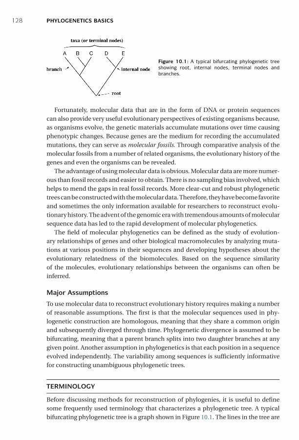
P1: IKB0521840988c10 CB1022/Xiong 0 521 84098 8 January 10, 2006 11:7
128 PHYLOGENETICS BASICS
Figure 10.1: A typical bifurcating phylogenetic treeshowing root, internal nodes, terminal nodes andbranches.
Fortunately, molecular data that are in the form of DNA or protein sequencescan also provide very useful evolutionary perspectives of existing organisms because,as organisms evolve, the genetic materials accumulate mutations over time causingphenotypic changes. Because genes are the medium for recording the accumulatedmutations, they can serve as molecular fossils. Through comparative analysis of themolecular fossils from a number of related organisms, the evolutionary history of thegenes and even the organisms can be revealed.
The advantage of using molecular data is obvious. Molecular data are more numer-ous than fossil records and easier to obtain. There is no sampling bias involved, whichhelps to mend the gaps in real fossil records. More clear-cut and robust phylogenetictrees can be constructed with the molecular data. Therefore, they have become favoriteand sometimes the only information available for researchers to reconstruct evolu-tionary history. The advent of the genomic era with tremendous amounts of molecularsequence data has led to the rapid development of molecular phylogenetics.
The field of molecular phylogenetics can be defined as the study of evolution-ary relationships of genes and other biological macromolecules by analyzing muta-tions at various positions in their sequences and developing hypotheses about theevolutionary relatedness of the biomolecules. Based on the sequence similarityof the molecules, evolutionary relationships between the organisms can often beinferred.
Major Assumptions
To use molecular data to reconstruct evolutionary history requires making a numberof reasonable assumptions. The first is that the molecular sequences used in phy-logenetic construction are homologous, meaning that they share a common originand subsequently diverged through time. Phylogenetic divergence is assumed to bebifurcating, meaning that a parent branch splits into two daughter branches at anygiven point. Another assumption in phylogenetics is that each position in a sequenceevolved independently. The variability among sequences is sufficiently informativefor constructing unambiguous phylogenetic trees.
TERMINOLOGY
Before discussing methods for reconstruction of phylogenies, it is useful to definesome frequently used terminology that characterizes a phylogenetic tree. A typicalbifurcating phylogenetic tree is a graph shown in Figure 10.1. The lines in the tree are
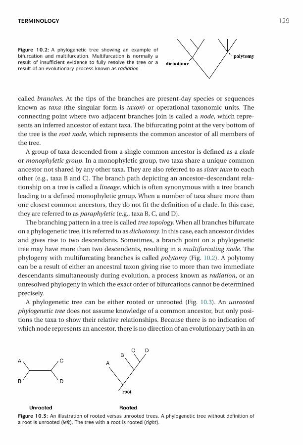
P1: IKB0521840988c10 CB1022/Xiong 0 521 84098 8 January 10, 2006 11:7
TERMINOLOGY 129
Figure 10.2: A phylogenetic tree showing an example ofbifurcation and multifurcation. Multifurcation is normally aresult of insufficient evidence to fully resolve the tree or aresult of an evolutionary process known as radiation.
called branches. At the tips of the branches are present-day species or sequencesknown as taxa (the singular form is taxon) or operational taxonomic units. Theconnecting point where two adjacent branches join is called a node, which repre-sents an inferred ancestor of extant taxa. The bifurcating point at the very bottom ofthe tree is the root node, which represents the common ancestor of all members ofthe tree.
A group of taxa descended from a single common ancestor is defined as a cladeor monophyletic group. In a monophyletic group, two taxa share a unique commonancestor not shared by any other taxa. They are also referred to as sister taxa to eachother (e.g., taxa B and C). The branch path depicting an ancestor–descendant rela-tionship on a tree is called a lineage, which is often synonymous with a tree branchleading to a defined monophyletic group. When a number of taxa share more thanone closest common ancestors, they do not fit the definition of a clade. In this case,they are referred to as paraphyletic (e.g., taxa B, C, and D).
The branching pattern in a tree is called tree topology. When all branches bifurcateon a phylogenetic tree, it is referred to as dichotomy. In this case, each ancestor dividesand gives rise to two descendants. Sometimes, a branch point on a phylogenetictree may have more than two descendents, resulting in a multifurcating node. Thephylogeny with multifurcating branches is called polytomy (Fig. 10.2). A polytomycan be a result of either an ancestral taxon giving rise to more than two immediatedescendants simultaneously during evolution, a process known as radiation, or anunresolved phylogeny in which the exact order of bifurcations cannot be determinedprecisely.
A phylogenetic tree can be either rooted or unrooted (Fig. 10.3). An unrootedphylogenetic tree does not assume knowledge of a common ancestor, but only posi-tions the taxa to show their relative relationships. Because there is no indication ofwhich node represents an ancestor, there is no direction of an evolutionary path in an
Figure 10.3: An illustration of rooted versus unrooted trees. A phylogenetic tree without definition ofa root is unrooted (left). The tree with a root is rooted (right).
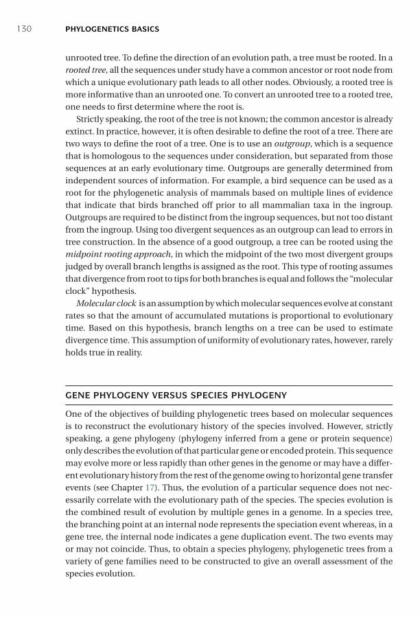
P1: IKB0521840988c10 CB1022/Xiong 0 521 84098 8 January 10, 2006 11:7
130 PHYLOGENETICS BASICS
unrooted tree. To define the direction of an evolution path, a tree must be rooted. In arooted tree, all the sequences under study have a common ancestor or root node fromwhich a unique evolutionary path leads to all other nodes. Obviously, a rooted tree ismore informative than an unrooted one. To convert an unrooted tree to a rooted tree,one needs to first determine where the root is.
Strictly speaking, the root of the tree is not known; the common ancestor is alreadyextinct. In practice, however, it is often desirable to define the root of a tree. There aretwo ways to define the root of a tree. One is to use an outgroup, which is a sequencethat is homologous to the sequences under consideration, but separated from thosesequences at an early evolutionary time. Outgroups are generally determined fromindependent sources of information. For example, a bird sequence can be used as aroot for the phylogenetic analysis of mammals based on multiple lines of evidencethat indicate that birds branched off prior to all mammalian taxa in the ingroup.Outgroups are required to be distinct from the ingroup sequences, but not too distantfrom the ingroup. Using too divergent sequences as an outgroup can lead to errors intree construction. In the absence of a good outgroup, a tree can be rooted using themidpoint rooting approach, in which the midpoint of the two most divergent groupsjudged by overall branch lengths is assigned as the root. This type of rooting assumesthat divergence from root to tips for both branches is equal and follows the “molecularclock” hypothesis.
Molecular clock is an assumption by which molecular sequences evolve at constantrates so that the amount of accumulated mutations is proportional to evolutionarytime. Based on this hypothesis, branch lengths on a tree can be used to estimatedivergence time. This assumption of uniformity of evolutionary rates, however, rarelyholds true in reality.
GENE PHYLOGENY VERSUS SPECIES PHYLOGENY
One of the objectives of building phylogenetic trees based on molecular sequencesis to reconstruct the evolutionary history of the species involved. However, strictlyspeaking, a gene phylogeny (phylogeny inferred from a gene or protein sequence)only describes the evolution of that particular gene or encoded protein. This sequencemay evolve more or less rapidly than other genes in the genome or may have a differ-ent evolutionary history from the rest of the genome owing to horizontal gene transferevents (see Chapter 17). Thus, the evolution of a particular sequence does not nec-essarily correlate with the evolutionary path of the species. The species evolution isthe combined result of evolution by multiple genes in a genome. In a species tree,the branching point at an internal node represents the speciation event whereas, in agene tree, the internal node indicates a gene duplication event. The two events mayor may not coincide. Thus, to obtain a species phylogeny, phylogenetic trees from avariety of gene families need to be constructed to give an overall assessment of thespecies evolution.
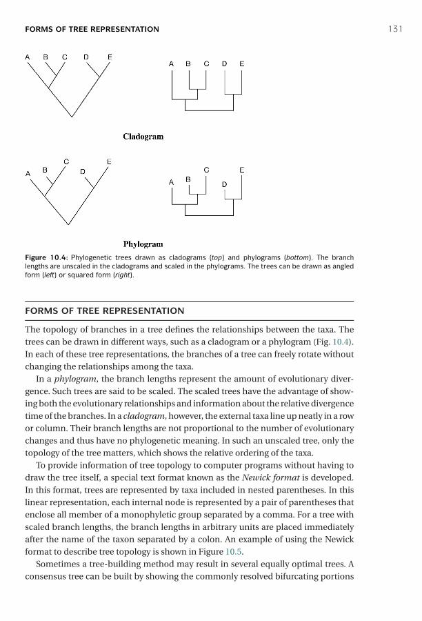
P1: IKB0521840988c10 CB1022/Xiong 0 521 84098 8 January 10, 2006 11:7
FORMS OF TREE REPRESENTATION 131
Figure 10.4: Phylogenetic trees drawn as cladograms (top) and phylograms (bottom). The branchlengths are unscaled in the cladograms and scaled in the phylograms. The trees can be drawn as angledform (left) or squared form (right).
FORMS OF TREE REPRESENTATION
The topology of branches in a tree defines the relationships between the taxa. Thetrees can be drawn in different ways, such as a cladogram or a phylogram (Fig. 10.4).In each of these tree representations, the branches of a tree can freely rotate withoutchanging the relationships among the taxa.
In a phylogram, the branch lengths represent the amount of evolutionary diver-gence. Such trees are said to be scaled. The scaled trees have the advantage of show-ing both the evolutionary relationships and information about the relative divergencetime of the branches. In a cladogram, however, the external taxa line up neatly in a rowor column. Their branch lengths are not proportional to the number of evolutionarychanges and thus have no phylogenetic meaning. In such an unscaled tree, only thetopology of the tree matters, which shows the relative ordering of the taxa.
To provide information of tree topology to computer programs without having todraw the tree itself, a special text format known as the Newick format is developed.In this format, trees are represented by taxa included in nested parentheses. In thislinear representation, each internal node is represented by a pair of parentheses thatenclose all member of a monophyletic group separated by a comma. For a tree withscaled branch lengths, the branch lengths in arbitrary units are placed immediatelyafter the name of the taxon separated by a colon. An example of using the Newickformat to describe tree topology is shown in Figure 10.5.
Sometimes a tree-building method may result in several equally optimal trees. Aconsensus tree can be built by showing the commonly resolved bifurcating portions
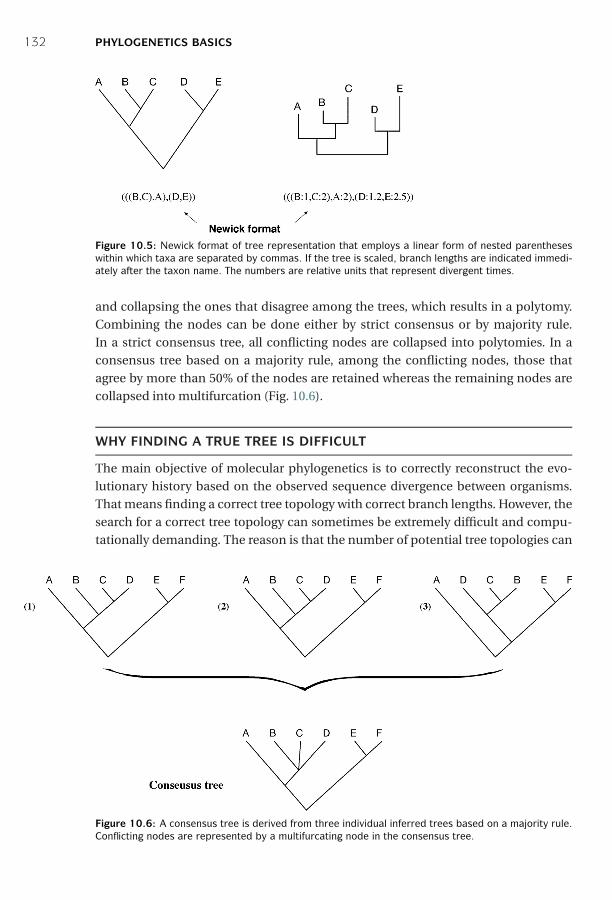
P1: IKB0521840988c10 CB1022/Xiong 0 521 84098 8 January 10, 2006 11:7
132 PHYLOGENETICS BASICS
Figure 10.5: Newick format of tree representation that employs a linear form of nested parentheseswithin which taxa are separated by commas. If the tree is scaled, branch lengths are indicated immedi-ately after the taxon name. The numbers are relative units that represent divergent times.
and collapsing the ones that disagree among the trees, which results in a polytomy.Combining the nodes can be done either by strict consensus or by majority rule.In a strict consensus tree, all conflicting nodes are collapsed into polytomies. In aconsensus tree based on a majority rule, among the conflicting nodes, those thatagree by more than 50% of the nodes are retained whereas the remaining nodes arecollapsed into multifurcation (Fig. 10.6).
WHY FINDING A TRUE TREE IS DIFFICULT
The main objective of molecular phylogenetics is to correctly reconstruct the evo-lutionary history based on the observed sequence divergence between organisms.That means finding a correct tree topology with correct branch lengths. However, thesearch for a correct tree topology can sometimes be extremely difficult and compu-tationally demanding. The reason is that the number of potential tree topologies can
Figure 10.6: A consensus tree is derived from three individual inferred trees based on a majority rule.Conflicting nodes are represented by a multifurcating node in the consensus tree.
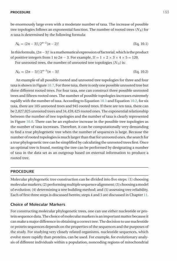
P1: IKB0521840988c10 CB1022/Xiong 0 521 84098 8 January 10, 2006 11:7
PROCEDURE 133
be enormously large even with a moderate number of taxa. The increase of possibletree topologies follows an exponential function. The number of rooted trees (N R) forn taxa is determined by the following formula:
NR = (2n − 3)!/2n−2(n − 2)! (Eq. 10.1)
In this formula, (2n−3)! is a mathematical expression of factorial, which is the productof positive integers from 1 to 2n − 3. For example, 5! = 1 × 2 × 3 × 4 × 5 = 120.
For unrooted trees, the number of unrooted tree topologies (N U) is:
NU = (2n − 5)!/2n−3(n − 3)! (Eq. 10.2)
An example of all possible rooted and unrooted tree topologies for three and fourtaxa is shown in Figure 10.7. For three taxa, there is only one possible unrooted tree butthree different rooted trees. For four taxa, one can construct three possible unrootedtrees and fifteen rooted ones. The number of possible topologies increases extremelyrapidly with the number of taxa. According to Equation 10.1 and Equation 10.2, for sixtaxa, there are 105 unrooted trees and 945 rooted trees. If there are ten taxa, there canbe 2,027,025 unrooted trees and 34,459,425 rooted ones. The exponential relationshipbetween the number of tree topologies and the number of taxa is clearly representedin Figure 10.8. There can be an explosive increase in the possible tree topologies asthe number of taxa increases. Therefore, it can be computationally very demandingto find a true phylogenetic tree when the number of sequences is large. Because thenumber of rooted topologies is much larger than that for unrooted ones, the search fora true phylogenetic tree can be simplified by calculating the unrooted trees first. Oncean optimal tree is found, rooting the tree can be performed by designating a numberof taxa in the data set as an outgroup based on external information to produce arooted tree.
PROCEDURE
Molecular phylogenetic tree construction can be divided into five steps: (1) choosingmolecular markers; (2) performing multiple sequence alignment; (3) choosing a modelof evolution; (4) determining a tree building method; and (5) assessing tree reliability.Each of first three steps is discussed herein; steps 4 and 5 are discussed in Chapter 11.
Choice of Molecular Markers
For constructing molecular phylogenetic trees, one can use either nucleotide or pro-tein sequence data. The choice of molecular markers is an important matter because itcan make a major difference in obtaining a correct tree. The decision to use nucleotideor protein sequences depends on the properties of the sequences and the purposes ofthe study. For studying very closely related organisms, nucleotide sequences, whichevolve more rapidly than proteins, can be used. For example, for evolutionary analy-sis of different individuals within a population, noncoding regions of mitochondrial
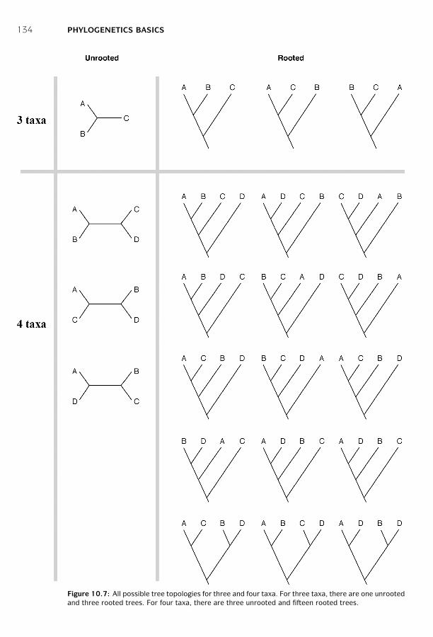
P1: IKB0521840988c10 CB1022/Xiong 0 521 84098 8 January 10, 2006 11:7
134 PHYLOGENETICS BASICS
Figure 10.7: All possible tree topologies for three and four taxa. For three taxa, there are one unrootedand three rooted trees. For four taxa, there are three unrooted and fifteen rooted trees.

P1: IKB0521840988c10 CB1022/Xiong 0 521 84098 8 January 10, 2006 11:7
PROCEDURE 135
Figure 10.8: Total number of rooted (◦) and unrooted (◆) tree topologies as a function of the numberof taxa. The values in the y-axis are plotted in the log scale.
DNA are often used. For studying the evolution of more widely divergent groups oforganisms, one may choose either slowly evolving nucleotide sequences, such as ribo-somal RNA or protein sequences. If the phylogenetic relationships to be delineatedare at the deepest level, such as between bacteria and eukaryotes, using conservedprotein sequences makes more sense than using nucleotide sequences. The reason isexplained in more detail next.
In many cases, protein sequences are preferable to nucleotide sequences becauseprotein sequences are relatively more conserved as a result of the degeneracy of thegenetic code in which sixty-one codons encode for twenty amino acids, meaningthereby a change in a codon may not result in a change in amino acid. Thus, proteinsequences can remain the same while the corresponding DNA sequences have moreroom for variation, especially at the third codon position. The significant differencein evolutionary rates among the three nucleotide positions also violates one of theassumptions of tree-building. In contrast, the protein sequences do not suffer fromthis problem, even for divergent sequences.
DNA sequences are sometimes more biased than protein sequences because ofpreferential codon usage in different organisms. In this case, different codons for thesame amino acid are used at different frequencies, leading to sequence variations notattributable to evolution. In addition, the genetic code of mitochondria varies fromthe standard genetic code. Therefore, for comparison of mitochondria protein-codinggenes, it is necessary to translate the DNA sequences into protein sequences.
P1: IKB0521840988c10 CB1022/Xiong 0 521 84098 8 January 10, 2006 11:7
136 PHYLOGENETICS BASICS
As mentioned in Chapter 4, protein sequences allow more sensitive alignment thanDNA sequences because the former has twenty characters versus four in the latter. Ithas been shown that two randomly related DNA sequences can result in up to 50%sequence identity when gaps are allowed compared to only 10% for protein sequences.For moderately divergent sequences, it is almost impossible to use DNA sequencesto obtain correct alignment. In addition, to align protein-coding DNA sequences,when gaps are introduced to maximize alignment scores, they almost always causeframeshift errors, making the alignment biologically meaningless. Protein sequencesclearly have a higher signal-to-noise ratio when it comes to alignment and phyloge-netic analysis. Thus, protein-based phylogeny in most cases may be more appropriatethan DNA-based phylogeny.
Despite the advantages of using protein sequences in phylogenetic inference, DNAsequences can still be very informative in some cases, such as those for closely relatedsequences. In this case, faster evolutionary rates at the DNA level become an advan-tage. In addition, DNA sequences depict synonymous and nonsynonymous substi-tutions, which can be useful for revealing evidence of positive or negative selectionevents.
To understand positive or negative selection, it is necessary to make a distinc-tion between synonymous substitutions and nonsynonymous substitutions. Syn-onymous substitutions are nucleotide changes in the coding sequence that do notresult in amino acid sequence changes for the encoded protein. Nonsynonymoussubstitutions are nucleotide changes that result in alterations in the amino acidsequences.
Comparing the two types of substitution rates helps to understand an evolutionaryprocess of a sequence. For example, if the nonsynonymous substitution rate is foundto be significantly greater than the synonymous substitution rate, this means thatcertain parts of the protein are undergoing active mutations that may contribute tothe evolution of new functions. This is described as positive selection or adaptiveevolution. On the other hand, if the synonymous substitution rate is greater than thenonsynonymous substitution rate, this causes only neutral changes at the amino acidlevel, suggesting that the protein sequence is critical enough that changes at the aminoacid sequence level are not tolerated. In this case, the sequence is said to be undernegative or purifying selection.
Alignment
The second step in phylogenetic analysis is to construct sequence alignment. Thisis probably the most critical step in the procedure because it establishes positionalcorrespondence in evolution. Only the correct alignment produces correct phyloge-netic inference because aligned positions are assumed to be genealogically related.Incorrect alignment leads to systematic errors in the final tree or even a completelywrong tree. For that reason, it is essential that the sequences are correctly aligned.Multiple state-of-the-art alignment programs such as T-Coffee should be used. Thealignment results from multiple sources should be inspected and compared carefully
P1: IKB0521840988c10 CB1022/Xiong 0 521 84098 8 January 10, 2006 11:7
PROCEDURE 137
to identify the most reasonable one. Automatic sequence alignments almost alwayscontain errors and should be further edited or refined if necessary.
Manual editing is often critical in ensuring alignment quality. However, there is nofirm rule on how to modify a sequence alignment. As a general guideline, a correctalignment should ensure the matching of key cofactor residues and residues of similarphysicochemical properties. If secondary structure elements are known or can bepredicted (see Chapter 14), they can serve to guide the alignment. One of the fewalignment programs that incorporates protein secondary structure information isPraline (see Chapter 5).
It is also often necessary to decide whether to use the full alignment or to extractparts of it. Truly ambiguously aligned regions have to be removed from considerationprior to phylogenetic analysis. Which part of the alignment to remove is often at thediscretion of the researcher. It is a rather subjective process. In extreme cases, someresearchers like to remove all insertions and deletions (indels) and only use positionsthat are shared by all sequences in the dataset. The clear drawback of this practice isthat many phylogenetic signals are lost. In fact, gap regions often belong to signatureindels unique to identification of a subgroup of sequences and should to be retainedfor treeing purposes.
In addition, there is an automatic approach in improving alignment quality. Rascaland NorMD (see Chapter 5) can help to improve alignment by correcting alignmenterrors and removing potentially unrelated or highly divergent sequences. Further-more, the program Gblocks (http://woody.embl-heidelberg.de/phylo/) can help todetect and eliminate the poorly aligned positions and divergent regions so to makethe alignment more suitable for phylogenetic analysis.
Multiple Substitutions
A simple measure of the divergence between two sequences is to count the number ofsubstitutions in an alignment. The proportion of substitutions defines the observeddistance between the two sequences. However, the observed number of substitutionsmay not represent the true evolutionary events that actually occurred. When a muta-tion is observed as A replaced by C, the nucleotide may have actually undergone anumber of intermediate steps to become C, such as A → T → G → C. Similarly, a backmutation could have occurred when a mutated nucleotide reverted back to the origi-nal nucleotide. This means that when the same nucleotide is observed, mutations likeG → C → G may have actually occurred. Moreover, an identical nucleotide observedin the alignment could be due to parallel mutations when both sequences mutate intoT, for instance.
Such multiple substitutions and convergence at individual positions obscure theestimation of the true evolutionary distances between sequences. This effect is knownas homoplasy, which, if not corrected, can lead to the generation of incorrect trees.To correct homoplasy, statistical models are needed to infer the true evolutionarydistances between sequences.
P1: IKB0521840988c10 CB1022/Xiong 0 521 84098 8 January 10, 2006 11:7
138 PHYLOGENETICS BASICS
Choosing Substitution Models
The statistical models used to correct homoplasy are called substitution models or evo-lutionary models. For constructing DNA phylogenies, there are a number of nucleotidesubstitution models available. These models differ in how multiple substitutions ofeach nucleotide are treated. The caveat of using these models is that if there aretoo many multiple substitutions at a particular position, which is often true for verydivergent sequences, the position may become saturated. This means that the evo-lutionary divergence is beyond the ability of the statistical models to correct. In thiscase, true evolutionary distances cannot be derived. Therefore, only reasonably sim-ilar sequences are to be used in phylogenetic comparisons.
Jukes–Cantor ModelThe simplest nucleotide substitution model is the Jukes–Cantor model, whichassumes that all nucleotides are substituted with equal probability. A formula forderiving evolutionary distances that include hidden changes is introduced by using alogarithmic function.
dAB = −(3/4) ln[1 − (4/3) pAB] (Eq. 10.3)
where d AB is the evolutionary distance between sequences A and B and p AB is theobserved sequence distance measured by the proportion of substitutions over theentire length of the alignment.
For example, if an alignment of sequences A and B is twenty nucleotides long andsix pairs are found to be different, the sequences differ by 30%, or have an observeddistance 0.3. To correct for multiple substitutions using the Jukes–Cantor model, thecorrected evolutionary distance based on Equation 10.3 is:
dAB = −3/4 ln[1 − (4/3 × 0.3)] = 0.38
The Jukes–Cantor model can only handle reasonably closely related sequences.According to Equation 10.3, the normalized distance increases as the actual observeddistance increases. For distantly related sequences, the correction can become toolarge to be reliable. If two DNA sequences have 25% similarity, p AB is 0.75. This leadsthe log value to be infinitely large.
Kimura ModelAnother model to correct evolutionary distances is called the Kimura two-parametermodel. This is a more sophisticated model in which mutation rates for transitionsand transversion are assumed to be different, which is more realistic. According tothis model, transitions occur more frequently than transversions, which, therefore,provides a more realistic estimate of evolutionary distances. The Kimura model usesthe following formula:
dAB = −(1/2) ln(1 − 2 pti − ptv) − (1/4) ln(1 − 2 ptv) (Eq. 10.4)

P1: IKB0521840988c10 CB1022/Xiong 0 521 84098 8 January 10, 2006 11:7
PROCEDURE 139
Figure 10.9: The Jukes–Cantor and Kimura models for DNA substitutions. In the Jukes–Cantor model,all nucleotides have equal substitution rates (α). In the Kimura model, there are unequal rates of tran-sitions (α) and transversions (β). The probability values for identical matches are shaded because evo-lutionary distances only count different residue positions.
where d AB is the evolutionary distance between sequences A and B, p ti is the observedfrequency for transition, and p tv the frequency of transversion. Comparison of theJukes–Cantor model and the Kimura model is graphically illustrated in Figure 10.9.
An example of using the Kimura model can be illustrated by the comparison ofsequences A and B that differ by 30%. If 20% of changes are a result of transitionsand 10% of changes are a result of transversions, the evolutionary distance can becalculated using Equation 10.4:
dAB = −1/2 ln(1 − 2 × 0.2 − 0.1) − 1/4 ln(1 − 2 × 0.1) = 0.40
In addition to these models, there are more complex models, such as TN93, HKY,and GTR, that take many more parameters into consideration. However, these morecomplex models are normally not used in practice because the calculations are toocomplicated and the variance levels resulting from the formula are too high.
For protein sequences, the evolutionary distances from an alignment can be cor-rected using a PAM or JTT amino acid substitution matrix whose construction alreadytakes into account the multiple substitutions (see Chapter 3). Alternatively, proteinequivalents of Jukes–Cantor and Kimura models can be used to correct evolutionarydistances. For example, the Kimura model for correcting multiple substitutions inprotein distances is:
d = −ln(1 − p − 0.2p2) (Eq. 10.5)
whereas p is the observed pairwise distance between two sequences.
Among-Site Variations
In all these calculations, different positions in a sequence are assumed to be evolvingat the same rate. However, this assumption may not hold up in reality. For example,in DNA sequences, the rates of substitution differ for different codon positions. Thethird codon mutates much faster than the other two. For protein sequences, someamino acids change much more rarely than others owing to functional constraints.This variation in evolutionary rates is the so-called among-site rate heterogeneity,which can also cause artifacts in tree construction.
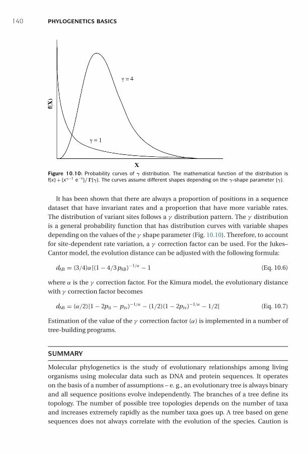
P1: IKB0521840988c10 CB1022/Xiong 0 521 84098 8 January 10, 2006 11:7
140 PHYLOGENETICS BASICS
Figure 10.10: Probability curves of γ distribution. The mathematical function of the distribution isf(x) + (xγ−1 e−x)/Γ(γ). The curves assume different shapes depending on the γ-shape parameter (γ).
It has been shown that there are always a proportion of positions in a sequencedataset that have invariant rates and a proportion that have more variable rates.The distribution of variant sites follows a γ distribution pattern. The γ distributionis a general probability function that has distribution curves with variable shapesdepending on the values of the γ shape parameter (Fig. 10.10). Therefore, to accountfor site-dependent rate variation, a γ correction factor can be used. For the Jukes–Cantor model, the evolution distance can be adjusted with the following formula:
dAB = (3/4)α[(1 − 4/3 pAB)−1/α − 1 (Eq. 10.6)
where α is the γ correction factor. For the Kimura model, the evolutionary distancewith γ correction factor becomes
dAB = (α/2)[1 − 2pti − ptv)−1/α − (1/2)(1 − 2ptv)−1/α − 1/2] (Eq. 10.7)
Estimation of the value of the γ correction factor (α) is implemented in a number oftree-building programs.
SUMMARY
Molecular phylogenetics is the study of evolutionary relationships among livingorganisms using molecular data such as DNA and protein sequences. It operateson the basis of a number of assumptions – e. g., an evolutionary tree is always binaryand all sequence positions evolve independently. The branches of a tree define itstopology. The number of possible tree topologies depends on the number of taxaand increases extremely rapidly as the number taxa goes up. A tree based on genesequences does not always correlate with the evolution of the species. Caution is

P1: IKB0521840988c10 CB1022/Xiong 0 521 84098 8 January 10, 2006 11:7
FURTHER READING 141
needed in extrapolation of phylogenetic results. A phylogenetic tree can be rooted orunrooted. The best way to root a tree is to use an outgroup, the selection of whichrelies on external knowledge. The first step in phylogenetic construction is to decidewhether to use DNA sequences or protein sequences, each having merits and limi-tations. Protein sequences are preferable in most cases. However, for studying veryrecent evolution, DNA is the marker of choice.
The second step is to perform multiple sequence alignment. Obtaining accuratealignment is critical for phylogenetic tree construction. The unique aspect of multi-ple alignment for phylogenetic analysis is that it often requires manual truncation ofambiguously aligned regions. The next step is to select a proper substitution modelthat provides estimates of the true evolutionary event by taking into account multiplesubstitution events. Corrected evolutionary distances are used both in distance-basedand likelihood-based tree-building methods. The commonly used nucleotide substi-tution models are the Jukes–Cantor and Kimura models. The commonly used aminoacid substitution models are the PAM and JTT models. Other adjustments to improvethe estimation of true evolutionary distances include the incorporation of rate het-erogeneity among sites.
FURTHER READING
Graur, D., and Li, W.-H. 2000. Fundamentals of Molecular Evolution. Sunderland, MA: SinauerAssociates.
Higgins, D. G. 2000. Amino acid-based phylogeny and alignment. Adv. Protein Chem. 54:99–135.Nei, M., and Kumar, S. 2000. Molecular Evolution and Phylogenetics. New York: Oxford Univer-
sity Press.Salemi, M., and Vandamme, A.-M. 2003. The Phylogenetics Handbook – A Practical Approach to
DNA and Protein Phylogeny. Cambridge, UK: Cambridge University Press.Thornton, J. W., and DeSalle, R. 2000. Gene family evolution and homology: Genomics meets
phylogenetics. Annu. Rev. Genomics Hum. Genet. 1:41–73.Whelan, S., Lio, P., and Goldman, N. 2001. Molecular phylogenetics: State of the art methods for
looking into the past. Trends Genet. 17:262–72.
P1: JZP0521840988c11 CB1022/Xiong 0 521 84098 8 January 10, 2006 14:54
CHAPTER ELEVEN
Phylogenetic Tree Construction Methodsand Programs
To continue discussion of molecular phylogenetics from Chapter 10, this chapterintroduces the theory behind various phylogenetic tree construction methods alongwith the strategies used for executing the tree construction.
There are currently two main categories of tree-building methods, each havingadvantages and limitations. The first category is based on discrete characters, whichare molecular sequences from individual taxa. The basic assumption is that charac-ters at corresponding positions in a multiple sequence alignment are homologousamong the sequences involved. Therefore, the character states of the common ances-tor can be traced from this dataset. Another assumption is that each character evolvesindependently and is therefore treated as an individual evolutionary unit. The secondcategory of phylogenetic methods is based on distance, which is the amount of dissim-ilarity between pairs of sequences, computed on the basis of sequence alignment. Thedistance-based methods assume that all sequences involved are homologous and thattree branches are additive, meaning that the distance between two taxa equals the sumof all branch lengths connecting them. More details on procedures and assumptionsfor each type of phylogenetic method are described.
DISTANCE-BASED METHODS
As mentioned in Chapter 10, true evolutionary distances between sequences canbe calculated from observed distances after correction using a variety of evolutionarymodels. The computed evolutionary distances can be used to construct a matrix of dis-tances between all individual pairs of taxa. Based on the pairwise distance scores in thematrix, a phylogenetic tree can be constructed for all the taxa involved. The algorithmsfor the distance-based tree-building method can be subdivided into either clusteringbased or optimality based. The clustering-type algorithms compute a tree based ona distance matrix starting from the most similar sequence pairs. These algorithmsinclude an unweighted pair group method using arithmetic average (UPGMA) andneighbor joining. The optimality-based algorithms compare many alternative treetopologies and select one that has the best fit between estimated distances in the treeand the actual evolutionary distances. This category includes the Fitch–Margoliashand minimum evolution algorithms.
142

P1: JZP0521840988c11 CB1022/Xiong 0 521 84098 8 January 10, 2006 14:54
DISTANCE-BASED METHODS 143
Clustering-Based Methods
Unweighted Pair Group Method Using Arithmetic AverageThe simplest clustering method is UPGMA, which builds a tree by a sequential cluster-ing method. Given a distance matrix, it starts by grouping two taxa with the smallestpairwise distance in the distance matrix. A node is placed at the midpoint or halfdistance between them. It then creates a reduced matrix by treating the new clusteras a single taxon. The distances between this new composite taxon and all remainingtaxa are calculated to create a reduced matrix. The same grouping process is repeatedand another newly reduced matrix is created. The iteration continues until all taxaare placed on the tree (see Box 11.1). The last taxon added is considered the outgroupproducing a rooted tree.
The basic assumption of the UPGMA method is that all taxa evolve at a constantrate and that they are equally distant from the root, implying that a molecular clock(see Chapter 10) is in effect. However, real data rarely meet this assumption. Thus,UPGMA often produces erroneous tree topologies. However, owing to its fast speedof calculation, it has found extensive usage in clustering analysis of DNA microarraydata (see Chapter 17).
Neighbor JoiningThe UPGMA method uses unweighted distances and assumes that all taxa have con-stant evolutionary rates. Since this molecular clock assumption is often not met inbiological sequences, to build a more accurate phylogenetic trees, the neighbor-joining (NJ) method can be used, which is somewhat similar to UPGMA in that itbuilds a tree by using stepwise reduced distance matrices. However, the NJ methoddoes not assume the taxa to be equidistant from the root. It corrects for unequalevolutionary rates between sequences by using a conversion step. This conversionrequires the calculations of “r-values” and “transformed r-values” using the followingformula:
d ′AB = dAB − 1/2 × (rA + rB) (Eq. 11.1)
where d ′AB is the converted distance between A and B and dAB is the actual evolutionary
distance between A and B. The value of rA (or rB) is the sum of distances of A (or B)to all other taxa. A generalized expression of the r-value is ri calculated based on thefollowing formula:
ri = �d ij (Eq. 11.2)
where i and j are two different taxa. The r-values are needed to create a modifieddistance matrix. The transformed r-values (r ′) are used to determine the distances ofan individual taxon to the nearest node.
r ′i = r i/n − 2 (Eq. 11.3)
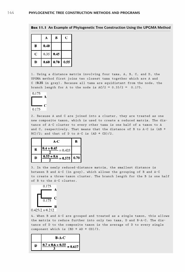
P1: JZP0521840988c11 CB1022/Xiong 0 521 84098 8 January 10, 2006 14:54
144 PHYLOGENETIC TREE CONSTRUCTION METHODS AND PROGRAMS
Box 11.1 An Example of Phylogenetic Tree Construction Using the UPGMA Method
1. Using a distance matrix involving four taxa, A, B, C, and D, theUPGMA method first joins two closest taxa together which are A andC (0.35 in grey). Because all taxa are equidistant from the node, thebranch length for A to the node is AC/2 = 0.35/2 = 0.175.
2. Because A and C are joined into a cluster, they are treated as onenew composite taxon, which is used to create a reduced matrix. The dis-tance of A–C cluster to every other taxa is one half of a taxon to Aand C, respectively. That means that the distance of B to A–C is (AB +BC)/2; and that of D to A–C is (AD + CD)/2.
3. In the newly reduced-distance matrix, the smallest distance isbetween B and A–C (in grey), which allows the grouping of B and A–Cto create a three-taxon cluster. The branch length for the B is one halfof B to the A–C cluster.
4. When B and A–C are grouped and treated as a single taxon, this allowsthe matrix to reduce further into only two taxa, D and B–A–C. The dis-tance of D to the composite taxon is the average of D to every singlecomponent which is (BD + AD + CD)/3.
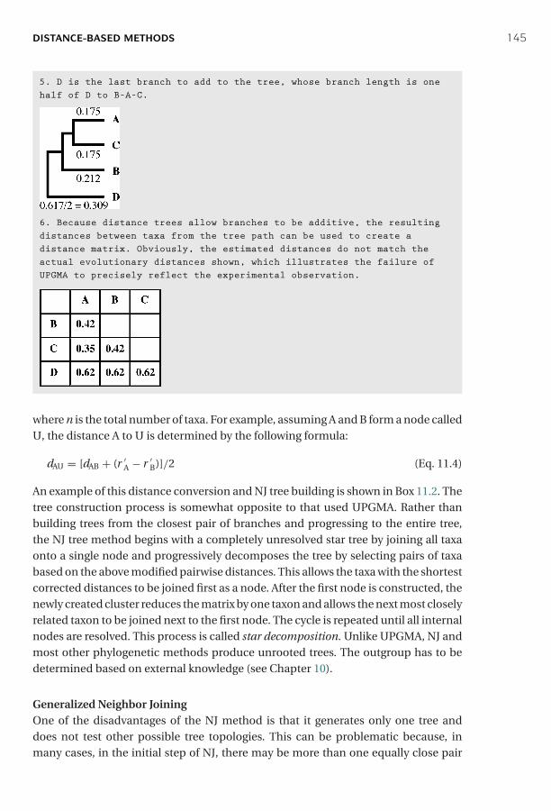
P1: JZP0521840988c11 CB1022/Xiong 0 521 84098 8 January 10, 2006 14:54
DISTANCE-BASED METHODS 145
5. D is the last branch to add to the tree, whose branch length is onehalf of D to B–A–C.
6. Because distance trees allow branches to be additive, the resultingdistances between taxa from the tree path can be used to create adistance matrix. Obviously, the estimated distances do not match theactual evolutionary distances shown, which illustrates the failure ofUPGMA to precisely reflect the experimental observation.
where n is the total number of taxa. For example, assuming A and B form a node calledU, the distance A to U is determined by the following formula:
dAU = [dAB + (r ′A − r ′
B)]/2 (Eq. 11.4)
An example of this distance conversion and NJ tree building is shown in Box 11.2. Thetree construction process is somewhat opposite to that used UPGMA. Rather thanbuilding trees from the closest pair of branches and progressing to the entire tree,the NJ tree method begins with a completely unresolved star tree by joining all taxaonto a single node and progressively decomposes the tree by selecting pairs of taxabased on the above modified pairwise distances. This allows the taxa with the shortestcorrected distances to be joined first as a node. After the first node is constructed, thenewly created cluster reduces the matrix by one taxon and allows the next most closelyrelated taxon to be joined next to the first node. The cycle is repeated until all internalnodes are resolved. This process is called star decomposition. Unlike UPGMA, NJ andmost other phylogenetic methods produce unrooted trees. The outgroup has to bedetermined based on external knowledge (see Chapter 10).
Generalized Neighbor JoiningOne of the disadvantages of the NJ method is that it generates only one tree anddoes not test other possible tree topologies. This can be problematic because, inmany cases, in the initial step of NJ, there may be more than one equally close pair
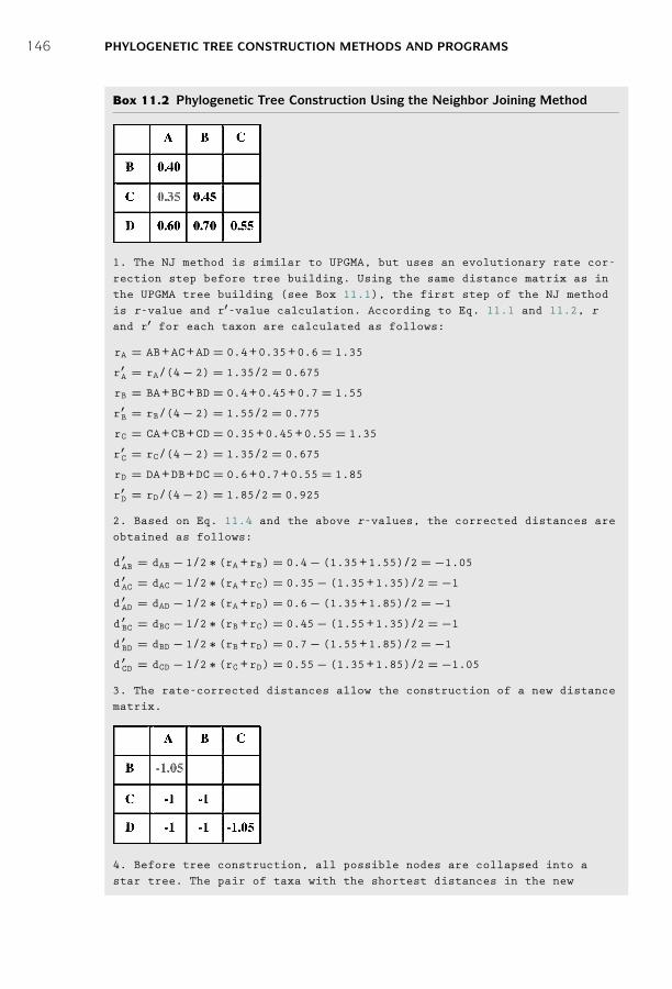
P1: JZP0521840988c11 CB1022/Xiong 0 521 84098 8 January 10, 2006 14:54
146 PHYLOGENETIC TREE CONSTRUCTION METHODS AND PROGRAMS
Box 11.2 Phylogenetic Tree Construction Using the Neighbor Joining Method
1. The NJ method is similar to UPGMA, but uses an evolutionary rate cor-rection step before tree building. Using the same distance matrix as inthe UPGMA tree building (see Box 11.1), the first step of the NJ methodis r-value and r′-value calculation. According to Eq. 11.1 and 11.2, rand r′ for each taxon are calculated as follows:
rA = AB+AC+AD = 0.4+0.35+0.6 = 1.35
r′A = rA/(4− 2) = 1.35/2 = 0.675
rB = BA+BC+BD = 0.4+0.45+0.7 = 1.55
r′B = rB/(4− 2) = 1.55/2 = 0.775
rC = CA+CB+CD = 0.35+0.45+0.55 = 1.35
r′C = rC/(4− 2) = 1.35/2 = 0.675
rD = DA+DB+DC = 0.6+0.7+0.55 = 1.85
r′D = rD/(4− 2) = 1.85/2 = 0.925
2. Based on Eq. 11.4 and the above r-values, the corrected distances areobtained as follows:
d ′AB = dAB − 1/2 ∗ (rA +rB) = 0.4− (1.35+1.55)/2 = −1.05
d ′AC = dAC − 1/2 ∗ (rA +rC) = 0.35− (1.35+1.35)/2 = −1
d ′AD = dAD − 1/2 ∗ (rA +rD) = 0.6− (1.35+1.85)/2 = −1
d ′BC = dBC − 1/2 ∗ (rB +rC) = 0.45− (1.55+1.35)/2 = −1
d ′BD = dBD − 1/2 ∗ (rB +rD) = 0.7− (1.55+1.85)/2 = −1
d ′CD = dCD − 1/2 ∗ (rC +rD) = 0.55− (1.35+1.85)/2 = −1.05
3. The rate-corrected distances allow the construction of a new distancematrix.
4. Before tree construction, all possible nodes are collapsed into astar tree. The pair of taxa with the shortest distances in the new

P1: JZP0521840988c11 CB1022/Xiong 0 521 84098 8 January 10, 2006 14:54
DISTANCE-BASED METHODS 147
matrix are separated from the star tree first, according to the cor-rected distances. In this case, A and B as well as C and D are theshortest (−1.05, in grey). Therefore, the first node to be built can beeither A–B or C–D. Choosing either pair first will give the same result.Let’s choose A and B first and name the node U.
5. The branch lengths for A and B to the node U are calculated accordingto Eq. 11.4.
dAU = [dAB +(r ′A − r ′
B)]/2 = [0.4+(0.675− 0.775)]/2 = 0.15
dBU = [dAB +(r ′B − r ′
A)]/2 = [0.4+(0.775− 0.675)]/2 = 0.25
6. The new cluster allows the construction of a reduced matrix. Thisstarts with actual distances. Unlike in UPGMA, the distance from a taxonto a node is the average of the original distances to each of the com-ponents of the composite taxon, subtracted from the inferred branchlengths.
dCU = [(dAC − dUA)+(dBC − dUB)]/2 = [(0.35− 0.15)+(0.45− 0.25)]/2 = 0.2
dDU = [(dAD − dUA)+(dBD − dUB)]/2 = [(0.6− 0.15)+(0.7− 0.25)]/2 = 0.45
7. Based on the reduced distance matrix, a new set of r- and r′-valuesare calculated.
rC = CU+CD = 0.2+0.55 = 0.75
r ′C = rC/(3− 2) = 0.75/1 = 0.75
rD = DU+CD = 0.45+0.55 = 1
r ′C = rC/(3− 2) = 1/1 = 1
rU = CU+DU = 0.2+0.45 = 0.65
r ′U = rU/(3− 2) = 0.65/1 = 0.65
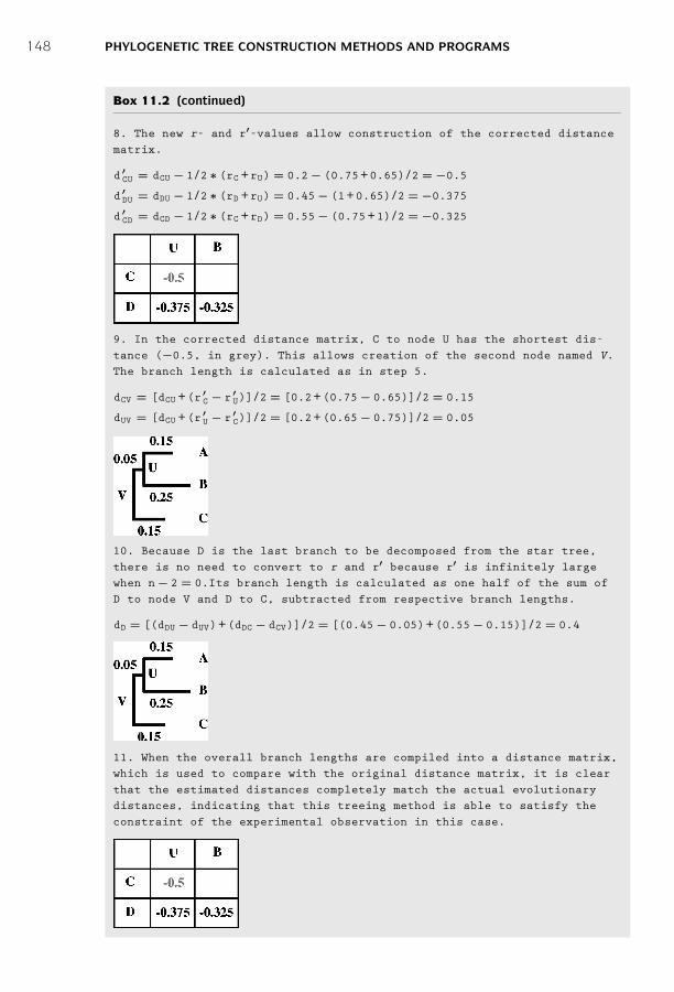
P1: JZP0521840988c11 CB1022/Xiong 0 521 84098 8 January 10, 2006 14:54
148 PHYLOGENETIC TREE CONSTRUCTION METHODS AND PROGRAMS
Box 11.2 (continued)
8. The new r- and r′-values allow construction of the corrected distancematrix.
d ′CU = dCU − 1/2 ∗ (rC +rU) = 0.2− (0.75+0.65)/2 = −0.5
d ′DU = dDU − 1/2 ∗ (rD +rU) = 0.45− (1+0.65)/2 = −0.375
d ′CD = dCD − 1/2 ∗ (rC +rD) = 0.55− (0.75+1)/2 = −0.325
9. In the corrected distance matrix, C to node U has the shortest dis-tance (−0.5, in grey). This allows creation of the second node named V.The branch length is calculated as in step 5.
dCV = [dCU +(r ′C − r ′
U)]/2 = [0.2+(0.75− 0.65)]/2 = 0.15
dUV = [dCU +(r ′U − r ′
C)]/2 = [0.2+(0.65− 0.75)]/2 = 0.05
10. Because D is the last branch to be decomposed from the star tree,there is no need to convert to r and r′ because r′ is infinitely largewhen n− 2 = 0.Its branch length is calculated as one half of the sum ofD to node V and D to C, subtracted from respective branch lengths.
dD = [(dDU − dUV)+(dDC − dCV)]/2 = [(0.45− 0.05)+(0.55− 0.15)]/2 = 0.4
11. When the overall branch lengths are compiled into a distance matrix,which is used to compare with the original distance matrix, it is clearthat the estimated distances completely match the actual evolutionarydistances, indicating that this treeing method is able to satisfy theconstraint of the experimental observation in this case.
P1: JZP0521840988c11 CB1022/Xiong 0 521 84098 8 January 10, 2006 14:54
DISTANCE-BASED METHODS 149
of neighbors to join, leading to multiple trees. Ignoring these multiple options mayyield a suboptimal tree. To overcome the limitations, a generalized NJ method hasbeen developed, in which multiple NJ trees with different initial taxon groupings aregenerated. A best tree is then selected from a pool of regular NJ trees that best fitthe actual evolutionary distances. This more extensive tree search means that thisapproach has a better chance of finding the correct tree.
Optimality-Based Methods
The clustering-based methods produce a single tree as output. However, there is nocriterion in judging how this tree is compared to other alternative trees. In contrast,optimality-based methods have a well-defined algorithm to compare all possible treetopologies and select a tree that best fits the actual evolutionary distance matrix.Based on the differences in optimality criteria, there are two types of algorithms,Fitch–Margoliash and minimum evolution, that are described next. The exhaustivesearch for an optimal tree necessitates a slow computation, which is a clear drawbackespecially when the dataset is large.
Fitch–MargoliashThe Fitch–Margoliash (FM) method selects a best tree among all possible trees basedon minimal deviation between the distances calculated in the overall branches in thetree and the distances in the original dataset. It starts by randomly clustering two taxain a node and creating three equations to describe the distances, and then solvingthe three algebraic equations for unknown branch lengths. The clustering of the twotaxa helps to create a newly reduced matrix. This process is iterated until a tree iscompletely resolved. The method searches for all tree topologies and selects the onethat has the lowest squared deviation of actual distances and calculated tree branchlengths. The optimality criterion is expressed in the following formula:
E =T−1∑i=1
T∑j=j + 1
(dij − pij)2
dij2
(Eq. 11.5)
where E is the error of the estimated tree fitting the original data, T is the number oftaxa, dij is the pairwise distance between ith and jth taxa in the original dataset, andpij is the corresponding tree branch length.
Minimum EvolutionMinimum evolution (ME) constructs a tree with a similar procedure, but uses a dif-ferent optimality criterion that finds a tree among all possible trees with a minimumoverall branch length. The optimality criterion relies on the formula:
S = �b i (Eq. 11.6)
where bi is the ith branch length. Searching for the minimum total branch length isan indirect approach to achieving the best fit of the branch lengths with the original
P1: JZP0521840988c11 CB1022/Xiong 0 521 84098 8 January 10, 2006 14:54
150 PHYLOGENETIC TREE CONSTRUCTION METHODS AND PROGRAMS
dataset. Analysis has shown that minimum evolution in fact slightly outperforms theleast square-based FM method.
Pros and Cons
The most frequently used distance methods are clustering based. The major advantageis that they are computationally fast and are therefore capable of handling datasetsthat are deemed to be too large for any other phylogenetic method. The methods, how-ever, are not guaranteed to find the best tree. Exhaustive tree-searching algorithmssuch as FM and ME have better accuracies overall. However, they can be compu-tationally prohibitive to use when the number of taxa is large (e.g., >12), becausethe overall number of tree topologies becomes too large to handle. A compromisebetween the two types of algorithm is a hybrid approach such as the generalized NJ,with a performance similar to that of ME but computationally much faster.
The overall advantage of all distance-based methods is the ability to make use ofa large number of substitution models to correct distances. The drawback is that theactual sequence information is lost when all the sequence variation is reduced to asingle value. Hence, ancestral sequences at internal nodes cannot be inferred.
CHARACTER-BASED METHODS
Character-based methods (also called discrete methods) are based directly on thesequence characters rather than on pairwise distances. They count mutational eventsaccumulated on the sequences and may therefore avoid the loss of informationwhen characters are converted to distances. This preservation of character informa-tion means that evolutionary dynamics of each character can be studied. Ancestralsequences can also be inferred. The two most popular character-based approachesare the maximum parsimony (MP) and maximum likelihood (ML) methods.
Maximum Parsimony
The parsimony method chooses a tree that has the fewest evolutionary changes orshortest overall branch lengths. It is based on a principle related to a medieval phi-losophy called Occam’s razor. The theory was formulated by William of Occam inthe thirteenth century and states that the simplest explanation is probably the cor-rect one. This is because the simplest explanation requires the fewest assumptionsand the fewest leaps of logic. In dealing with problems that may have an infinitenumber of possible solutions, choosing the simplest model may help to “shave off”those variables that are not really necessary to explain the phenomenon. By doingthis, model development may become easier, and there may be less chance of intro-ducing inconsistencies, ambiguities, and redundancies, hence, the name Occam’srazor.
For phylogenetic analysis, parsimony seems a good assumption. By this principle,a tree with the least number of substitutions is probably the best to explain the differ-ences among the taxa under study. This view is justified by the fact that evolutionary

P1: JZP0521840988c11 CB1022/Xiong 0 521 84098 8 January 10, 2006 14:54
CHARACTER-BASED METHODS 151
Figure 11.1: Example of identification of informativesites that are used in parsimony analysis. Sites 2, 5,and 8 (grey boxes) are informative sites. Other sitesare noninformative sites, which are either constantor having characters occurring only once.
changes are relatively rare within a reasonably short time frame. This implies that atree with minimal changes is likely to be a good estimate of the true tree. By minimizingthe changes, the method minimizes the phylogenetic noise owing to homoplasy andindependent evolution. The MP approach is in principle similar to the ME approachalbeit the latter is distance based instead of character based.
How Does MP Tree Building Work?Parsimony tree building works by searching for all possible tree topologies and recon-structing ancestral sequences that require the minimum number of changes to evolveto the current sequences. To save computing time, only a small number of sites thathave the richest phylogenetic information are used in tree determination. These sitesare the so-called informative sites, which are defined as sites that have at least two dif-ferent kinds of characters, each occurring at least twice (Fig. 11.1). Informative sitesare the ones that can often be explained by a unique tree topology. Other sites arenoninformative, which are constant sites or sites that have changes occurring onlyonce. Constant sites have the same state in all taxa and are obviously useless in evalu-ating the various topologies. The sites that have changes occurring only once are notvery useful either for constructing parsimony trees because they can be explained bymultiple tree topologies. The noninformative sites are thus discarded in parsimonytree construction.
Once the informative sites are identified and the noninformative sites discarded,the minimum number of substitutions at each informative site is computed for agiven tree topology. The total number of changes at all informative sites are summedup for each possible tree topology. The tree that has the smallest number of changesis chosen as the best tree.
The key to counting a minimum number of substitutions for a particular site is todetermine the ancestral character states at internal nodes. Because these ancestralcharacter states are not known directly, multiple possible solutions may exist. In thiscase, the parsimony principle applies to choose the character states that result in aminimum number of substitutions. The inference of an ancestral sequence is madeby first going from the leaves to internal nodes and to the common root to deter-mine all possible ancestral character states and then going back from the commonroot to the leaves to assign ancestral sequences that require the minimum number ofsubstitutions. An example of predicting ancestral sequences at internal nodes is given
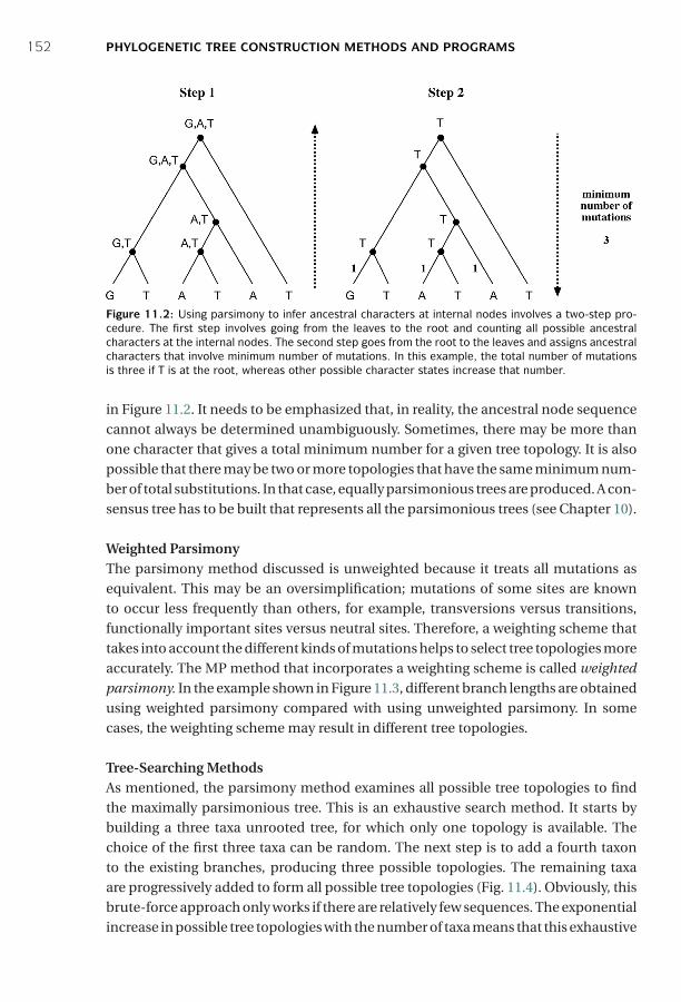
P1: JZP0521840988c11 CB1022/Xiong 0 521 84098 8 January 10, 2006 14:54
152 PHYLOGENETIC TREE CONSTRUCTION METHODS AND PROGRAMS
Figure 11.2: Using parsimony to infer ancestral characters at internal nodes involves a two-step pro-cedure. The first step involves going from the leaves to the root and counting all possible ancestralcharacters at the internal nodes. The second step goes from the root to the leaves and assigns ancestralcharacters that involve minimum number of mutations. In this example, the total number of mutationsis three if T is at the root, whereas other possible character states increase that number.
in Figure 11.2. It needs to be emphasized that, in reality, the ancestral node sequencecannot always be determined unambiguously. Sometimes, there may be more thanone character that gives a total minimum number for a given tree topology. It is alsopossible that there may be two or more topologies that have the same minimum num-ber of total substitutions. In that case, equally parsimonious trees are produced. A con-sensus tree has to be built that represents all the parsimonious trees (see Chapter 10).
Weighted ParsimonyThe parsimony method discussed is unweighted because it treats all mutations asequivalent. This may be an oversimplification; mutations of some sites are knownto occur less frequently than others, for example, transversions versus transitions,functionally important sites versus neutral sites. Therefore, a weighting scheme thattakes into account the different kinds of mutations helps to select tree topologies moreaccurately. The MP method that incorporates a weighting scheme is called weightedparsimony. In the example shown in Figure 11.3, different branch lengths are obtainedusing weighted parsimony compared with using unweighted parsimony. In somecases, the weighting scheme may result in different tree topologies.
Tree-Searching MethodsAs mentioned, the parsimony method examines all possible tree topologies to findthe maximally parsimonious tree. This is an exhaustive search method. It starts bybuilding a three taxa unrooted tree, for which only one topology is available. Thechoice of the first three taxa can be random. The next step is to add a fourth taxonto the existing branches, producing three possible topologies. The remaining taxaare progressively added to form all possible tree topologies (Fig. 11.4). Obviously, thisbrute-force approach only works if there are relatively few sequences. The exponentialincrease in possible tree topologies with the number of taxa means that this exhaustive
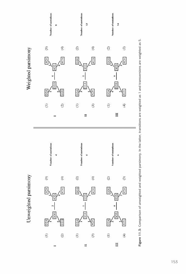
P1: JZP0521840988c11 CB1022/Xiong 0 521 84098 8 January 10, 2006 14:54
Figu
re1
1.3
:C
ompar
ison
ofun
wei
ghte
dan
dw
eigh
ted
par
sim
ony.
Inth
ela
tter
,tr
ansi
tion
sar
ew
eigh
ted
as1
and
tran
sver
sion
sar
ew
eigh
ted
as5.
153
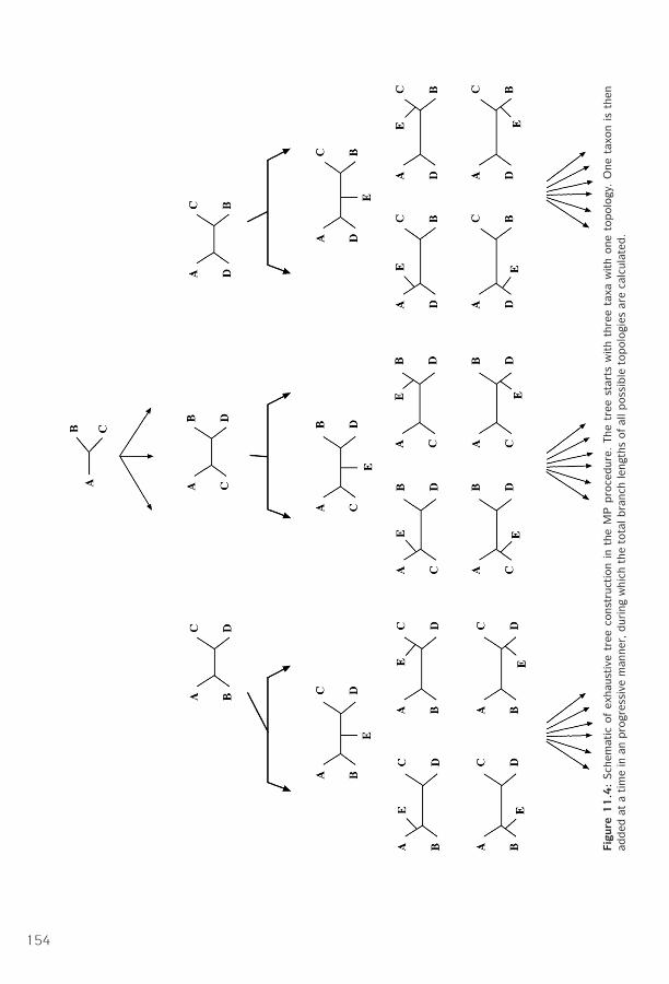
P1: JZP0521840988c11 CB1022/Xiong 0 521 84098 8 January 10, 2006 14:54
Figu
re1
1.4
:Sch
emat
icof
exha
ustive
tree
cons
truc
tion
inth
eM
Ppro
cedur
e.Th
etr
eest
arts
with
thre
eta
xaw
ith
one
topol
ogy.
One
taxo
nis
then
added
ata
tim
ein
anpro
gres
sive
man
ner,
dur
ing
whi
chth
eto
talb
ranc
hle
ngth
sof
allp
ossi
ble
topol
ogie
sar
eca
lcul
ated
.
154
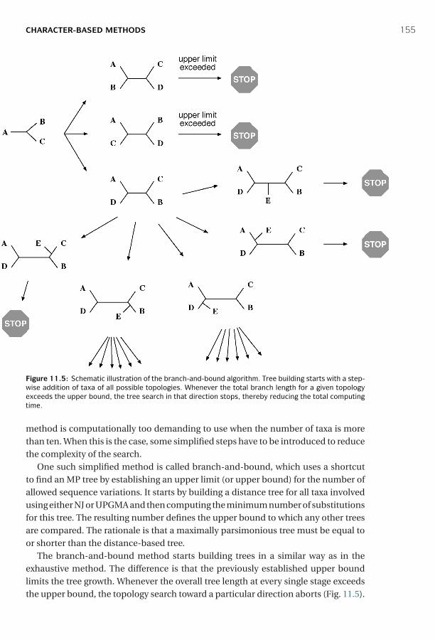
P1: JZP0521840988c11 CB1022/Xiong 0 521 84098 8 January 10, 2006 14:54
CHARACTER-BASED METHODS 155
Figure 11.5: Schematic illustration of the branch-and-bound algorithm. Tree building starts with a step-wise addition of taxa of all possible topologies. Whenever the total branch length for a given topologyexceeds the upper bound, the tree search in that direction stops, thereby reducing the total computingtime.
method is computationally too demanding to use when the number of taxa is morethan ten. When this is the case, some simplified steps have to be introduced to reducethe complexity of the search.
One such simplified method is called branch-and-bound, which uses a shortcutto find an MP tree by establishing an upper limit (or upper bound) for the number ofallowed sequence variations. It starts by building a distance tree for all taxa involvedusing either NJ or UPGMA and then computing the minimum number of substitutionsfor this tree. The resulting number defines the upper bound to which any other treesare compared. The rationale is that a maximally parsimonious tree must be equal toor shorter than the distance-based tree.
The branch-and-bound method starts building trees in a similar way as in theexhaustive method. The difference is that the previously established upper boundlimits the tree growth. Whenever the overall tree length at every single stage exceedsthe upper bound, the topology search toward a particular direction aborts (Fig. 11.5).
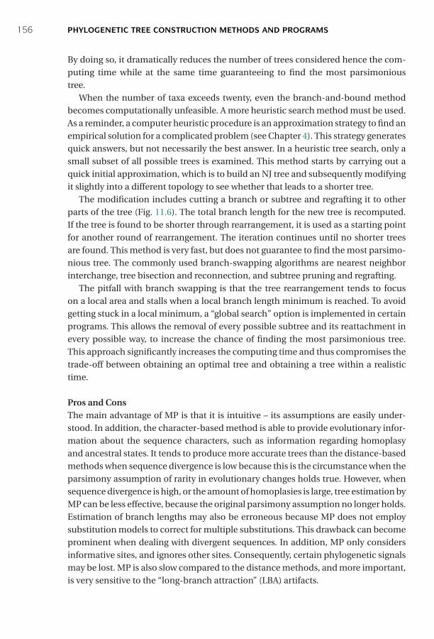
P1: JZP0521840988c11 CB1022/Xiong 0 521 84098 8 January 10, 2006 14:54
156 PHYLOGENETIC TREE CONSTRUCTION METHODS AND PROGRAMS
By doing so, it dramatically reduces the number of trees considered hence the com-puting time while at the same time guaranteeing to find the most parsimonioustree.
When the number of taxa exceeds twenty, even the branch-and-bound methodbecomes computationally unfeasible. A more heuristic search method must be used.As a reminder, a computer heuristic procedure is an approximation strategy to find anempirical solution for a complicated problem (see Chapter 4). This strategy generatesquick answers, but not necessarily the best answer. In a heuristic tree search, only asmall subset of all possible trees is examined. This method starts by carrying out aquick initial approximation, which is to build an NJ tree and subsequently modifyingit slightly into a different topology to see whether that leads to a shorter tree.
The modification includes cutting a branch or subtree and regrafting it to otherparts of the tree (Fig. 11.6). The total branch length for the new tree is recomputed.If the tree is found to be shorter through rearrangement, it is used as a starting pointfor another round of rearrangement. The iteration continues until no shorter treesare found. This method is very fast, but does not guarantee to find the most parsimo-nious tree. The commonly used branch-swapping algorithms are nearest neighborinterchange, tree bisection and reconnection, and subtree pruning and regrafting.
The pitfall with branch swapping is that the tree rearrangement tends to focuson a local area and stalls when a local branch length minimum is reached. To avoidgetting stuck in a local minimum, a “global search” option is implemented in certainprograms. This allows the removal of every possible subtree and its reattachment inevery possible way, to increase the chance of finding the most parsimonious tree.This approach significantly increases the computing time and thus compromises thetrade-off between obtaining an optimal tree and obtaining a tree within a realistictime.
Pros and ConsThe main advantage of MP is that it is intuitive – its assumptions are easily under-stood. In addition, the character-based method is able to provide evolutionary infor-mation about the sequence characters, such as information regarding homoplasyand ancestral states. It tends to produce more accurate trees than the distance-basedmethods when sequence divergence is low because this is the circumstance when theparsimony assumption of rarity in evolutionary changes holds true. However, whensequence divergence is high, or the amount of homoplasies is large, tree estimation byMP can be less effective, because the original parsimony assumption no longer holds.Estimation of branch lengths may also be erroneous because MP does not employsubstitution models to correct for multiple substitutions. This drawback can becomeprominent when dealing with divergent sequences. In addition, MP only considersinformative sites, and ignores other sites. Consequently, certain phylogenetic signalsmay be lost. MP is also slow compared to the distance methods, and more important,is very sensitive to the “long-branch attraction” (LBA) artifacts.
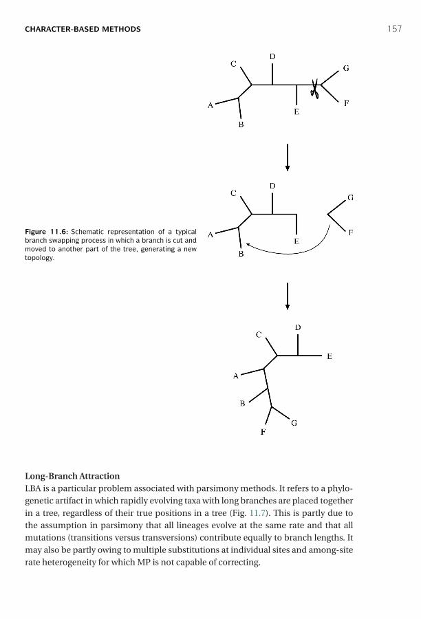
P1: JZP0521840988c11 CB1022/Xiong 0 521 84098 8 January 10, 2006 14:54
CHARACTER-BASED METHODS 157
Figure 11.6: Schematic representation of a typicalbranch swapping process in which a branch is cut andmoved to another part of the tree, generating a newtopology.
Long-Branch AttractionLBA is a particular problem associated with parsimony methods. It refers to a phylo-genetic artifact in which rapidly evolving taxa with long branches are placed togetherin a tree, regardless of their true positions in a tree (Fig. 11.7). This is partly due tothe assumption in parsimony that all lineages evolve at the same rate and that allmutations (transitions versus transversions) contribute equally to branch lengths. Itmay also be partly owing to multiple substitutions at individual sites and among-siterate heterogeneity for which MP is not capable of correcting.

P1: JZP0521840988c11 CB1022/Xiong 0 521 84098 8 January 10, 2006 14:54
158 PHYLOGENETIC TREE CONSTRUCTION METHODS AND PROGRAMS
Figure 11.7: The LBA artifact showing taxa A and D are artifactually clustered during phylogeneticconstruction.
There are several possible solutions to the LBA artifact. For homoplasies that causeLBA, distance and likelihood (discussed below) methods that employ substitutionmodels and rate heterogeneity models should be able to alleviate the problem. Inaddition, weighted parsimony should be more advantageous than unweighted par-simony in countering the transitional bias when transitions occur more often thantransversions. Increasing the taxon sampling size may also help because introduc-tion of intermediate taxa breaks up the long branches. A dataset with concatenatedmultiple genes also has less chance of LBA because the combined gene analysis maydampen the effect of a single gene having a high rate of evolution.
Maximum Likelihood Method
Another character-based approach is ML, which uses probabilistic models to choosea best tree that has the highest probability or likelihood of reproducing the observeddata. It finds a tree that most likely reflects the actual evolutionary process. ML is anexhaustive method that searches every possible tree topology and considers everyposition in an alignment, not just informative sites. By employing a particular substi-tution model that has probability values of residue substitutions, ML calculates thetotal likelihood of ancestral sequences evolving to internal nodes and eventually toexisting sequences. It sometimes also incorporates parameters that account for ratevariations across sites.
How Does the Maximum Likelihood Method Work?ML works by calculating the probability of a given evolutionary path for a particu-lar extant sequence. The probability values are determined by a substitution model(either for nucleotides or amino acids). For example, for DNA sequences using theJukes–Cantor model, the probability (P ) that a nucleotide remains the same aftertime t is:
P(t) = 1/4 + 3/4e−αt (Eq. 11.7)
where α is the nucleotide substitution rate in the Jukes–Cantor model, which is eitherempirically assigned or estimated from the raw datasets. In Figure 11.8, the elapsedtime t from X to A can be assigned as 1 and from Z to A as 2. For a nucleotide tochange into a different residue after time t, the probability value is determined by the
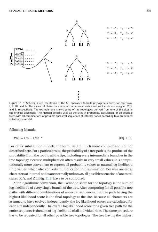
P1: JZP0521840988c11 CB1022/Xiong 0 521 84098 8 January 10, 2006 14:54
CHARACTER-BASED METHODS 159
Figure 11.8: Schematic representation of the ML approach to build phylogenetic trees for four taxa,I, II, III, and IV. The ancestral character states at the internal nodes and root node are assigned X, Y,and Z, respectively. The example only shows some of the topologies derived from one of the sites inthe original alignment. The method actually uses all the sites in probability calculation for all possibletrees with all combinations of possible ancestral sequences at internal nodes according to a predefinedsubstitution model.
following formula:
P(t) = 1/4 − 1/4e−αt (Eq. 11.8)
For other substitution models, the formulas are much more complex and are notdescribed here. For a particular site, the probability of a tree path is the product of theprobability from the root to all the tips, including every intermediate branches in thetree topology. Because multiplication often results in very small values, it is compu-tationally more convenient to express all probability values as natural log likelihood(lnL) values, which also converts multiplication into summation. Because ancestralcharacters at internal nodes are normally unknown, all possible scenarios of ancestralstates (X, Y, and Z in Fig. 11.8) have to be computed.
After logarithmic conversion, the likelihood score for the topology is the sum oflog likelihood of every single branch of the tree. After computing for all possible treepaths with different combinations of ancestral sequences, the tree path having thehighest likelihood score is the final topology at the site. Because all characters areassumed to have evolved independently, the log likelihood scores are calculated foreach site independently. The overall log likelihood score for a given tree path for theentire sequence is the sum of log likelihood of all individual sites. The same procedurehas to be repeated for all other possible tree topologies. The tree having the highest
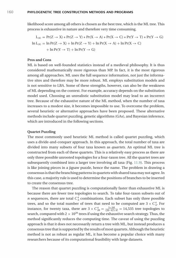
P1: JZP0521840988c11 CB1022/Xiong 0 521 84098 8 January 10, 2006 14:54
160 PHYLOGENETIC TREE CONSTRUCTION METHODS AND PROGRAMS
likelihood score among all others is chosen as the best tree, which is the ML tree. Thisprocess is exhaustive in nature and therefore very time consuming.
L(4) = Pr(Z → X) ∗ Pr(Z → Y) ∗ Pr(X → A) ∗ Pr(X → C) ∗ Pr(Y → T) ∗ Pr(Y → G)
ln L(4) = ln Pr(Z → X) + ln Pr(Z → Y) + ln Pr(X → A) + ln Pr(X → C)
+ ln Pr(Y → T) + ln Pr(Y → G)
Pros and ConsML is based on well-founded statistics instead of a medieval philosophy. It is thusconsidered mathematically more rigorous than MP. In fact, it is the most rigorousamong all approaches. ML uses the full sequence information, not just the informa-tive sites and therefore may be more robust. ML employs substitution models andis not sensitive to LBA. Some of these strengths, however, can also be the weaknessof ML depending on the context. For example, accuracy depends on the substitutionmodel used. Choosing an unrealistic substitution model may lead to an incorrecttree. Because of the exhaustive nature of the ML method, when the number of taxaincreases to a modest size, it becomes impossible to use. To overcome the problem,several heuristic or alternative approaches have been proposed. These alternativemethods include quartet puzzling, genetic algorithms (GAs), and Bayesian inference,which are introduced in the following sections.
Quartet PuzzlingThe most commonly used heuristic ML method is called quartet puzzling, whichuses a divide-and-conquer approach. In this approach, the total number of taxa aredivided into many subsets of four taxa known as quartets. An optimal ML tree isconstructed from each of these quartets. This is a relatively easy process as there areonly three possible unrooted topologies for a four-taxon tree. All the quartet trees aresubsequently combined into a larger tree involving all taxa (Fig. 11.9). This processis like joining pieces in a jigsaw puzzle, hence the name. The problem in drawing aconsensus is that the branching patterns in quartets with shared taxa may not agree. Inthis case, a majority rule is used to determine the positions of branches to be insertedto create the consensus tree.
The reason that quartet puzzling is computationally faster than exhaustive ML isbecause there are fewer tree topologies to search. To take four-taxon subsets out ofn sequences, there are total C 4
n combinations. Each subset has only three possibletrees, and so the total number of trees that need to be computed are 3 × C 4
n. Forinstance, for twenty taxa, there are 3 × C 4
20 = 3×20!(20−4)!×4! = 14,535 tree topologies to
search, compared with 2 × 10²⁰ trees if using the exhaustive search strategy. Thus, themethod significantly reduces the computing time. The caveat of using the puzzlingapproach is that it does not necessarily return a tree with ML, but instead produces aconsensus tree that is supported by the results of most quartets. Although the heuristicmethod is not as robust as regular ML, it has become a popular choice with manyresearchers because of its computational feasibility with large datasets.
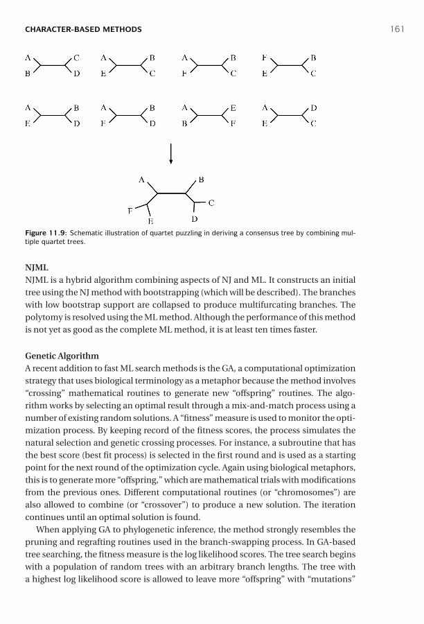
P1: JZP0521840988c11 CB1022/Xiong 0 521 84098 8 January 10, 2006 14:54
CHARACTER-BASED METHODS 161
Figure 11.9: Schematic illustration of quartet puzzling in deriving a consensus tree by combining mul-tiple quartet trees.
NJMLNJML is a hybrid algorithm combining aspects of NJ and ML. It constructs an initialtree using the NJ method with bootstrapping (which will be described). The brancheswith low bootstrap support are collapsed to produce multifurcating branches. Thepolytomy is resolved using the ML method. Although the performance of this methodis not yet as good as the complete ML method, it is at least ten times faster.
Genetic AlgorithmA recent addition to fast ML search methods is the GA, a computational optimizationstrategy that uses biological terminology as a metaphor because the method involves“crossing” mathematical routines to generate new “offspring” routines. The algo-rithm works by selecting an optimal result through a mix-and-match process using anumber of existing random solutions. A “fitness” measure is used to monitor the opti-mization process. By keeping record of the fitness scores, the process simulates thenatural selection and genetic crossing processes. For instance, a subroutine that hasthe best score (best fit process) is selected in the first round and is used as a startingpoint for the next round of the optimization cycle. Again using biological metaphors,this is to generate more “offspring,” which are mathematical trials with modificationsfrom the previous ones. Different computational routines (or “chromosomes”) arealso allowed to combine (or “crossover”) to produce a new solution. The iterationcontinues until an optimal solution is found.
When applying GA to phylogenetic inference, the method strongly resembles thepruning and regrafting routines used in the branch-swapping process. In GA-basedtree searching, the fitness measure is the log likelihood scores. The tree search beginswith a population of random trees with an arbitrary branch lengths. The tree witha highest log likelihood score is allowed to leave more “offspring” with “mutations”
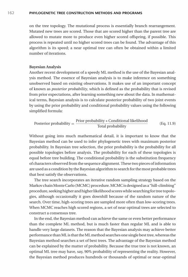
P1: JZP0521840988c11 CB1022/Xiong 0 521 84098 8 January 10, 2006 14:54
162 PHYLOGENETIC TREE CONSTRUCTION METHODS AND PROGRAMS
on the tree topology. The mutational process is essentially branch rearrangement.Mutated new trees are scored. Those that are scored higher than the parent tree areallowed to mutate more to produce even higher scored offspring, if possible. Thisprocess is repeated until no higher scored trees can be found. The advantage of thisalgorithm is its speed; a near optimal tree can often be obtained within a limitednumber of iterations.
Bayesian AnalysisAnother recent development of a speedy ML method is the use of the Bayesian anal-ysis method. The essence of Bayesian analysis is to make inference on somethingunobserved based on existing observations. It makes use of an important conceptof known as posterior probability, which is defined as the probability that is revisedfrom prior expectations, after learning something new about the data. In mathemat-ical terms, Bayesian analysis is to calculate posterior probability of two joint eventsby using the prior probability and conditional probability values using the followingsimplified formula:
Posterior probability = Prior probability ∗ Conditional likelihoodTotal probability
(Eq. 11.9)
Without going into much mathematical detail, it is important to know that theBayesian method can be used to infer phylogenetic trees with maximum posteriorprobability. In Bayesian tree selection, the prior probability is the probability for allpossible topologies before analysis. The probability for each of these topologies isequal before tree building. The conditional probability is the substitution frequencyof characters observed from the sequence alignment. These two pieces of informationare used as a condition by the Bayesian algorithm to search for the most probable treesthat best satisfy the observations.
The tree search incorporates an iterative random sampling strategy based on theMarkov chain Monte Carlo (MCMC) procedure. MCMC is designed as a “hill-climbing”procedure, seeking higher and higher likelihood scores while searching for tree topolo-gies, although occasionally it goes downhill because of the random nature of thesearch. Over time, high-scoring trees are sampled more often than low-scoring trees.When MCMC reaches high scored regions, a set of near optimal trees are selected toconstruct a consensus tree.
In the end, the Bayesian method can achieve the same or even better performancethan the complete ML method, but is much faster than regular ML and is able tohandle very large datasets. The reason that the Bayesian analysis may achieve betterperformance than ML is that the ML method searches one single best tree, whereas theBayesian method searches a set of best trees. The advantage of the Bayesian methodcan be explained by the matter of probability. Because the true tree is not known, anoptimal ML tree may have, say, 90% probability of representing the reality. However,the Bayesian method produces hundreds or thousands of optimal or near-optimal
P1: JZP0521840988c11 CB1022/Xiong 0 521 84098 8 January 10, 2006 14:54
PHYLOGENETIC TREE EVALUATION 163
trees with 88% to 90% probability to represent the reality. Thus, the latter approachhas a better chance overall to guess the true tree correctly.
PHYLOGENETIC TREE EVALUATION
After phylogenetic tree construction, the next step is to statistically evaluate the reli-ability of the inferred phylogeny. There are two questions that need to be addressed.One is how reliable the tree or a portion of the tree is; and the second is whetherthis tree is significantly better than another tree. To answer the first question, weneed to use analytical resampling strategies such as bootstrapping and jackknifing,which repeatedly resample data from the original dataset. For the second question,conventional statistical tests are needed.
What Is Bootstrapping?
Bootstrapping is a statistical technique that tests the sampling errors of a phyloge-netic tree. It does so by repeatedly sampling trees through slightly perturbed datasets.By doing so, the robustness of the original tree can be assessed. The rationale forbootstrapping is that a newly constructed tree is possibly biased owing to incor-rect alignment or chance fluctuations of distance measurements. To determine therobustness or reproducibility of the current tree, trees are repeatedly constructed withslightly perturbed alignments that have some random fluctuations introduced. A trulyrobust phylogenetic relationship should have enough characters to support the rela-tionship even if the dataset is perturbed in such a way. Otherwise, the noise introducedin the resampling process is sufficient to generate different trees, indicating that theoriginal topology may be derived from weak phylogenetic signals. Thus, this type ofanalysis gives an idea of the statistical confidence of the tree topology.
Parametric and Nonparametric Bootstrapping
Bootstrap resampling relies on perturbation of original sequence datasets. There aretwo perturbation strategies. One way to produce perturbations is through randomreplacement of sites. This is referred to as nonparametric bootstrapping. Alternatively,new datasets can be generated based on a particular sequence distribution, which isparametric bootstrapping. Both types of bootstrapping can be applied to the distance,parsimony, and likelihood tree construction methods.
In nonparametric bootstrapping, a new multiple sequence alignment of the samelength is generated with random duplication of some of the sites (i.e., the columnsin an alignment) at the expense of some other sites. In other words, certain sites arerandomly replaced by other existing sites. Consequently, certain sites may appearmultiple times, and other sites may not appear at all in the new alignment (Fig. 11.10).This process is repeated 100 to 1,000 times to create 100 to 1,000 new alignments thatare used to reconstruct phylogenetic trees using the same method as the originallyinferred tree. The new datasets with altered the nucleotide or amino acid composition
P1: JZP0521840988c11 CB1022/Xiong 0 521 84098 8 January 10, 2006 14:54
164 PHYLOGENETIC TREE CONSTRUCTION METHODS AND PROGRAMS
Figure 11.10: Schematic representation of a bootstrap analysis showing the original alignment andmodified replicates in which certain sites are randomly replaced with other existing sites. The resultingaltered replicates are used to building trees for statistical analysis at each node.
and rate heterogeneity may result in certain parts of the tree having a different topo-logy from the original inferred tree.
All the bootstrapped trees are summarized into a consensus tree based on a majo-rity rule. The most supported branching patterns shown at each node are labeled withbootstrap values, which are the percentage of appearance of a particular clade. Thus,the bootstrap test provides a measure for evaluating the confidence levels of the treetopology. Analysis has shown that a bootstrap value of 70% approximately corres-ponds to 95% statistical confidence, although the issue is still a subject of debate.
Instead of randomly duplicating sites to generate new datasets, parametric boot-strapping uses altered datasets with random sequences confined within a particularsequence distribution according to a given substitution model. For instance, for anucleotide dataset, according to the Juke–Cantor model, all four nucleotides are iden-tically distributed, whereas the Kimura model provides a different distribution (seeFig. 10.8). The parametric bootstrapping method may help avoid the problem of cer-tain sites being repeated too many times as in nonparametric bootstrapping resulting
P1: JZP0521840988c11 CB1022/Xiong 0 521 84098 8 January 10, 2006 14:54
PHYLOGENETIC TREE EVALUATION 165
in skewed sequence distribution. If a correct nucleotide/amino acid distributionmodel is used, parametric bootstrapping generates more reasonable replicates thanrandom replicates. Thus, this procedure is considered more robust than nonparamet-ric bootstrapping.
Caveats
Strictly speaking, bootstrapping does not assess the accuracy of a tree, but onlyindicates consistency and stability of individual clades of the tree. This means that,because of systematic errors, wrong trees can still be obtained with high bootstrapvalues. Therefore, bootstrap results should be interpreted with caution. Unusuallyhigh GC content in the original dataset, unusually accelerated evolutionary rates andunrealistic evolutionary models are the potential causes for generating biased trees,as well as biased bootstrap estimates, which come after the tree generation.
In addition, from a statistical point of view, a large number of bootstrap resamplingsteps are needed to achieve meaningful results. It is generally recommended that aphylogenetic tree should be bootstrapped 500 to 1,000 times. However, this presents apractical dilemma. In many instances, it may take hours or days to construct one MLor MP tree. So the multiplication of computing time makes bootstrapping virtuallyimpossible to use with limited computing resources.
Jackknifing
In addition to bootstrapping, another often used resampling technique is jackknif-ing. In jackknifing, one half of the sites in a dataset are randomly deleted, creatingdatasets half as long as the original. Each new dataset is subjected to phylogenetictree construction using the same method as the original. The advantage of jackknifingis that sites are not duplicated relative to the original dataset and that computing timeis much shortened because of shorter sequences. One criticism of this approach isthat the size of datasets has been changed into one half and that the datasets are nolonger considered replicates. Thus, the results may not be comparable with that frombootstrapping.
Bayesian Simulation
In terms of statistical evaluation, the Bayesian method is probably the most efficient;it does not require bootstrapping because the MCMC procedure itself involves thou-sands or millions of steps of resampling. As a result of Bayesian tree construction,posterior probabilities are assigned at each node of a best Bayesian tree as statisticalsupport. Because of fast computational speed of MCMC tree searching, the Bayesianmethod offers a practical advantage over regular ML and makes the statistical eval-uation of ML trees more feasible. Unlike bootstrap values, Bayesian probabilities arenormally higher because most trees are sampled near a small number of optimal trees.Therefore, they have a different statistical meaning from bootstrap.
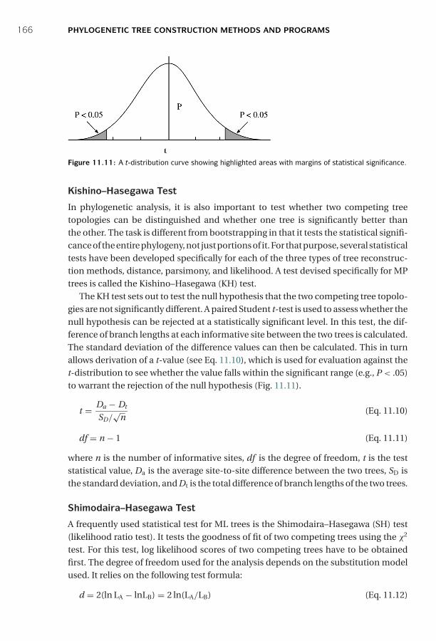
P1: JZP0521840988c11 CB1022/Xiong 0 521 84098 8 January 10, 2006 14:54
166 PHYLOGENETIC TREE CONSTRUCTION METHODS AND PROGRAMS
Figure 11.11: A t-distribution curve showing highlighted areas with margins of statistical significance.
Kishino–Hasegawa Test
In phylogenetic analysis, it is also important to test whether two competing treetopologies can be distinguished and whether one tree is significantly better thanthe other. The task is different from bootstrapping in that it tests the statistical signifi-cance of the entire phylogeny, not just portions of it. For that purpose, several statisticaltests have been developed specifically for each of the three types of tree reconstruc-tion methods, distance, parsimony, and likelihood. A test devised specifically for MPtrees is called the Kishino–Hasegawa (KH) test.
The KH test sets out to test the null hypothesis that the two competing tree topolo-gies are not significantly different. A paired Student t-test is used to assess whether thenull hypothesis can be rejected at a statistically significant level. In this test, the dif-ference of branch lengths at each informative site between the two trees is calculated.The standard deviation of the difference values can then be calculated. This in turnallows derivation of a t-value (see Eq. 11.10), which is used for evaluation against thet-distribution to see whether the value falls within the significant range (e.g., P < .05)to warrant the rejection of the null hypothesis (Fig. 11.11).
t = Da − Dt
SD/√
n(Eq. 11.10)
df = n − 1 (Eq. 11.11)
where n is the number of informative sites, df is the degree of freedom, t is the teststatistical value, Da is the average site-to-site difference between the two trees, SD isthe standard deviation, and Dt is the total difference of branch lengths of the two trees.
Shimodaira–Hasegawa Test
A frequently used statistical test for ML trees is the Shimodaira–Hasegawa (SH) test(likelihood ratio test). It tests the goodness of fit of two competing trees using the χ2
test. For this test, log likelihood scores of two competing trees have to be obtainedfirst. The degree of freedom used for the analysis depends on the substitution modelused. It relies on the following test formula:
d = 2(ln LA − lnLB) = 2 ln(LA/LB) (Eq. 11.12)
P1: JZP0521840988c11 CB1022/Xiong 0 521 84098 8 January 10, 2006 14:54
PHYLOGENETIC PROGRAMS 167
where d is the log likelihood ratio score and lnLA and lnLB are likelihood scores fortree A and tree B, respectively. The statistical meaning of d can be obtained fromcalculating the probability value from a χ2 table.
Once the log ratio of the two scores is obtained, it is used to test against the χ2 distri-bution. The resulting probability value (P-value) determines whether the differencebetween the two trees is significant.
PHYLOGENETIC PROGRAMS
Phylogenetic tree reconstruction is not a trivial task. Although there are numerousphylogenetic programs available, knowing the theoretical background, capabilities,and limitations of each is very important. For a list of hundreds of phylogenetic soft-ware programs, see Felsenstein’s collection at: http://evolution.genetics.washington.edu/phylip/software.html. Most of these programs are freely available. Some are com-prehensive packages; others are more specialized to perform a single task. Most requirespecial efforts to learn how to use them effectively. Because this book is not intendedas a computer manual, a brief introduction to several of the most commonly usedprograms is provided.
PAUP* (Phylogenetic analysis using parsimony and other methods, by DavidSwofford, http://paup.csit.fsu.edu/) is a commercial phylogenetic package. It is prob-ably one of the most widely used phylogenetic programs available from Sinauer Pub-lishers. It is a Macintosh program (UNIX version available in the GCG package) with avery user-friendly graphical interface. PAUP was originally developed as a parsimonyprogram, but expanded to a comprehensive package that is capable of performingdistance, parsimony, and likelihood analyses. The distance options include NJ, ME,FM, and UPGMA. For distance or ML analyses, PAUP has the option for detailed speci-fications of substitution models, base frequencies, and among site rate heterogeneity(γ -shape parameters, proportion of invariant sites). PAUP is also able to performnonparametric bootstrapping, jackknifing, KH testing, and SH testing.
Phylip (Phylogenetic inference package; by Joe Felsenstein) is a free multiplatformcomprehensive package containing thirty-five subprograms for performing distance,parsimony, and likelihood analysis, as well as bootstrapping for both nucleotide andamino acid sequences. It is command-line based, but relatively easy to use for eachsingle program. The only problem is that to complete an analysis the user is requiredto move between different subprograms while keeping modifying names of the inter-mediate output files. The program package is downloadable from http://evolution.genetics.washington.edu/phylip.html. An online version is also available at http://bioweb.pasteur.fr/seqanal/phylogeny/phylip-uk.html. A more user-friendly onlineversion is WebPhylip available at http://sdmc.krdl.org.sg:8080/∼lxzhang/phylip/.
TREE-PUZZLE is a program performing quartet puzzling. The advantage is thatit allows various substitution models for likelihood score estimation and incorpo-rates a discrete γ model for rate heterogeneity among sites (see Chapter 10). Becauseof the heuristic nature of the program, it allows ML analyses of large datasets. The
P1: JZP0521840988c11 CB1022/Xiong 0 521 84098 8 January 10, 2006 14:54
168 PHYLOGENETIC TREE CONSTRUCTION METHODS AND PROGRAMS
resulting puzzle trees are automatically assigned puzzle support values to internalbranches. These values are percentages of consistent quartet trees and do not havethe same meaning as bootstrap values. TREE-PUZZLE version 5.0 is available forMac, UNIX, and Windows and can be downloaded from www.tree-puzzle.de/. Thereis also an online version of the program available at: http://bioweb.pasteur.fr/seqanal/interfaces/Puzzle.html.
PHYML (http://atgc.lirmm.fr/phyml/) is a web-based phylogenetic program usingthe GA. It first builds an NJ tree and uses it as a starting tree for subsequent itera-tive refinement through subtree swapping. Branch lengths are simultaneously opti-mized during this process. The tree searching stops when the total ML score no longerincreases. The main advantage of this program is the ability to build trees from verylarge datasets with hundreds of taxa and to complete tree searching within a relativelyshort time frame.
MrBayes is a Bayesian phylogenetic inference program. It randomly samples treetopologies using the MCMC procedure and infers the posterior distribution of treetopologies. It has a range of probabilistic models available to search for a set oftrees with the highest posterior probability. It is fast and capable of handling largedatasets. The program is available in multiplatform versions and can be downloadedfrom http://morphbank.ebc.uu.se/mrbayes/. A web program that also employsBayesian inference for phylogenetic analysis is BAMBE (http://bioweb.pasteur.fr/seqanal/interfaces/bambe.html).
SUMMARY
Molecular phylogeny is a fundamental tool for understanding sequence evolution andrelationships. The accuracy of the tree-building methods used for phylogenetic anal-ysis depends on the assumption on which each the method is based. Understandingthese assumptions is the first step toward efficient use of these methods. The secondstep is understanding how the methods actually work and what intrinsic limitationsthese methods have. The third step is choosing suitable phylogenetic method(s) thatcan give a reasonably correct picture of a phylogenetic tree.
The phylogenetic methods can be divided into distance-based and character-basedmethods. The distance methods include UPGMA, NJ, Fitch–Margoliash, and min-imum evolution. The first two are clustering based, and are fast but not accurate;the latter two are optimality based and are accurate but not fast. Character-basedapproaches include the MP and ML methods. The principle of parsimony is easy tounderstand, but has its root in a medieval philosophy. It is slower compared to distancemethods. To speed up the computation, branch-and-bound and heuristics treesearching strategies are used. The ML method is the slowest, but is based on a solidstatistical foundation. To overcome the bottleneck of computation in ML, faster algo-rithms such as quartet puzzling, NJML, GA, and Bayesian analysis have been devel-oped to make the method more feasible. To assess the reliability and robustness of
P1: JZP0521840988c11 CB1022/Xiong 0 521 84098 8 January 10, 2006 14:54
FURTHER READING 169
every clade in a phylogenetic tree, bootstrapping and jackknifing are used. The KHand SH tests distinguish the overall topology of two competing trees.
It is important to realize that phylogenetic tree reconstruction is not a trivial matter,but a complicated process that often requires careful thought. Accuracy, reliability,and computational speed are all major factors for consideration when choosing aparticular phylogenetic method. It is also important to realize that none of the threephylogenetic reconstruction methods are guaranteed to find the correct tree. All threemethods have the potential to produce erroneous trees. To minimize phylogeneticerrors, it is recommended that at least two methods be used for any phylogeneticanalysis to check the consistency of tree building results obtained. Because the the-ories behind each of the three methods are fundamentally different, agreement inconclusion by several of these methods provides a particularly strong support for acorrect phylogenetic tree. In addition, it is recommended that different rate substitu-tion models, weighting schemes, and resampling strategies with or without exclusionof specific taxa and/or sites be applied. The same analysis should be repeated onmultiple genes or proteins as well as the concatenated datasets. If more than onefundamentally different methods provide the same prediction, the confidence in theprediction is higher.
FURTHER READING
Graur, D., and Li, W.-H. 2000. Fundamentals of Molecular Evolution. Sunderland, MA: SinauerAssociates.
Hall, B. G. 2001. Phylogenetic Trees Made Easy. A How-to Manual for Molecular Biologists.Sunderland, MA: Sinauer Associates.
Huelsenbeck J. P., Ronquist, F., Nielsen R., and Bollback, J. P. 2001. Bayesian inference of phy-logeny and its impact on evolutionary biology. Science. 294:2310–14.
Nei, M., and Kumar, S. 2000. Molecular Evolution and Phylogenetics. New York: Oxford UniversityPress.
Salemi, M., and Vandamme, A.-M. 2003. The Phylogenetics Handbook – A Practical Approach toDNA and Protein Phylogeny. Cambridge, UK: Cambridge University Press.
Swofford, D. L., Olsen, G. J., Waddel, P. J., and Hillis, D. M. 1996. ”Phylogenetic inference.” InMolecular Systematics. 2nd ed., edited by D. M. Hillis, C. Moritz, and B. K. Mable Sunderland,MA: Sinauer Associates.

P1: JZP0521840988c11 CB1022/Xiong 0 521 84098 8 January 10, 2006 14:54
170

P1: IKB0521840988c12 CB1022/Xiong 0 521 84098 8 January 10, 2006 13:45
SECTION FIVE
Structural Bioinformatics
171

P1: IKB0521840988c12 CB1022/Xiong 0 521 84098 8 January 10, 2006 13:45
172
P1: IKB0521840988c12 CB1022/Xiong 0 521 84098 8 January 10, 2006 13:45
CHAPTER TWELVE
Protein Structure Basics
Starting from this chapter and continuing through the next three chapters, we intro-duce the basics of protein structural bioinformatics. Proteins perform most essentialbiological and chemical functions in a cell. They play important roles in structural,enzymatic, transport, and regulatory functions. The protein functions are strictlydetermined by their structures. Therefore, protein structural bioinformatics is anessential element of bioinformatics. This chapter covers some basics of protein struc-tures and associated databases, preparing the reader for discussions of more advancedtopics of protein structural bioinformatics.
AMINO ACIDS
The building blocks of proteins are twenty naturally occurring amino acids, smallmolecules that contain a free amino group (NH2) and a free carboxyl group (COOH).Both of these groups are linked to a central carbon (Cα), which is attached to a hydro-gen and a side chain group (R) (Fig. 12.1). Amino acids differ only by the side chain Rgroup. The chemical reactivities of the R groups determine the specific properties ofthe amino acids.
Amino acids can be grouped into several categories based on the chemical andphysical properties of the side chains, such as size and affinity for water. According tothese properties, the side chain groups can be divided into small, large, hydrophobic,and hydrophilic categories. Within the hydrophobic set of amino acids, they can befurther divided into aliphatic and aromatic. Aliphatic side chains are linear hydro-carbon chains and aromatic side chains are cyclic rings. Within the hydrophilic set,amino acids can be subdivided into polar and charged. Charged amino acids can beeither positively charged (basic) or negatively charged (acidic). Each of the twentyamino acids, their abbreviations, and main functional features once incorporatedinto a protein are listed in Table 12.1.
Of particular interest within the twenty amino acids are glycine and proline.Glycine, the smallest amino acid, has a hydrogen atom as the R group. It can there-fore adopt more flexible conformations that are not possible for other amino acids.Proline is on the other extreme of flexibility. Its side chain forms a bond with itsown backbone amino group, causing it to be cyclic. The cyclic conformation makesit very rigid, unable to occupy many of the main chain conformations adopted byother amino acids. In addition, certain amino acids are subject to modifications after
173
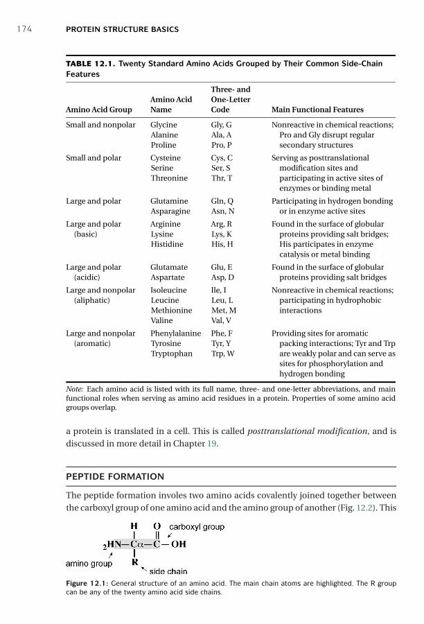
P1: IKB0521840988c12 CB1022/Xiong 0 521 84098 8 January 10, 2006 13:45
174 PROTEIN STRUCTURE BASICS
TABLE 12.1. Twenty Standard Amino Acids Grouped by Their Common Side-ChainFeatures
Three- andAmino Acid One-Letter
Amino Acid Group Name Code Main Functional Features
Small and nonpolar GlycineAlanineProline
Gly, GAla, APro, P
Nonreactive in chemical reactions;Pro and Gly disrupt regularsecondary structures
Small and polar CysteineSerineThreonine
Cys, CSer, SThr, T
Serving as posttranslationalmodification sites andparticipating in active sites ofenzymes or binding metal
Large and polar GlutamineAsparagine
Gln, QAsn, N
Participating in hydrogen bondingor in enzyme active sites
Large and polar(basic)
ArginineLysineHistidine
Arg, RLys, KHis, H
Found in the surface of globularproteins providing salt bridges;His participates in enzymecatalysis or metal binding
Large and polar(acidic)
GlutamateAspartate
Glu, EAsp, D
Found in the surface of globularproteins providing salt bridges
Large and nonpolar(aliphatic)
IsoleucineLeucineMethionineValine
Ile, ILeu, LMet, MVal, V
Nonreactive in chemical reactions;participating in hydrophobicinteractions
Large and nonpolar(aromatic)
PhenylalanineTyrosineTryptophan
Phe, FTyr, YTrp, W
Providing sites for aromaticpacking interactions; Tyr and Trpare weakly polar and can serve assites for phosphorylation andhydrogen bonding
Note: Each amino acid is listed with its full name, three- and one-letter abbreviations, and mainfunctional roles when serving as amino acid residues in a protein. Properties of some amino acidgroups overlap.
a protein is translated in a cell. This is called posttranslational modification, and isdiscussed in more detail in Chapter 19.
PEPTIDE FORMATION
The peptide formation involes two amino acids covalently joined together betweenthe carboxyl group of one amino acid and the amino group of another (Fig. 12.2). This
Figure 12.1: General structure of an amino acid. The main chain atoms are highlighted. The R groupcan be any of the twenty amino acid side chains.

P1: IKB0521840988c12 CB1022/Xiong 0 521 84098 8 January 10, 2006 13:45
DIHEDRAL ANGLES 175
Figure 12.2: Condensation reaction between the carboxyl group of one amino acid and the amino groupof another. The hydroxyl group of the carboxyl group and a hydrogen of the amino group are lost togive rise to a water molecule and a dipeptide.
reaction is a condensation reaction involving removal of elements of water from thetwo molecules. The resulting product is called a dipeptide. The newly formed covalentbond connecting the two amino acids is called a peptide bond. Once an amino acid isincorporated into a peptide, it becomes an amino acid residue. Multiple amino acidscan be joined together to form a longer chain of amino acid polymer.
A linear polymer of more than fifty amino acid residues is referred to as a polypep-tide. A polypeptide, also called a protein, has a well-defined three-dimensionalarrangement. On the other hand, a polymer with fewer than fifty residues is usuallycalled a peptide without a well-defined three-dimensional structure. The residues ina peptide or polypeptide are numbered beginning with the residue containing theamino group, referred to as the N-terminus, and ending with the residue containingthe carboxyl group, known as the C-terminus (see Fig. 12.2). The actual sequence ofamino acid residues in a polypeptide determines its ultimate structure and function.
The atoms involved in forming the peptide bond are referred to as the backboneatoms. They are the nitrogen of the amino group, the α carbon to which the side chainis attached and carbon of the carbonyl group.
DIHEDRAL ANGLES
A peptide bond is actually a partial double bond owing to shared electrons betweenO=C–N atoms. The rigid double bond structure forces atoms associated with thepeptide bond to lie in the same plane, called the peptide plane. Because of the planarnature of the peptide bond and the size of the R groups, there are considerable restric-tions on the rotational freedom by the two bonded pairs of atoms around the peptidebond. The angle of rotation about the bond is referred to as the dihedral angle (alsocalled the tortional angle).
For a peptide unit, the atoms linked to the peptide bond can be moved to a certainextent by the rotation of two bonds flanking the peptide bond. This is measured bytwo dihedral angles (Fig. 12.3). One is the dihedral angle along the N–Cα bond, whichis defined as phi (φ); and the other is the angle along the Cα–C bond, which is calledpsi (ψ). Various combinations of φ and ψ angles allow the proteins to fold in manydifferent ways.
Ramachandran Plot
As mentioned, the rotation of φ and ψ is not completely free because of the planarnature of the peptide bond and the steric hindrance from the side chain R group.
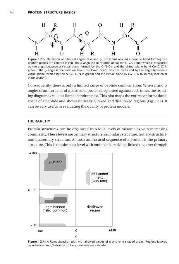
P1: IKB0521840988c12 CB1022/Xiong 0 521 84098 8 January 10, 2006 13:45
176 PROTEIN STRUCTURE BASICS
Figure 12.3: Definition of dihedral angles of φ and ψ. Six atoms around a peptide bond forming twopeptide planes are colored in red. The φ angle is the rotation about the N–Cα bond, which is measuredby the angle between a virtual plane formed by the C–N–Cα and the virtual plane by N–Cα–C (C ingreen). The ψ angle is the rotation about the Cα–C bond, which is measured by the angle between avirtual plane formed by the N–Cα–C (N in green) and the virtual plane by Cα–C–N (N in red) (see colorplate section).
Consequently, there is only a limited range of peptide conformation. When φ and ψ
angles of amino acids of a particular protein are plotted against each other, the result-ing diagram is called a Ramachandran plot. This plot maps the entire conformationalspace of a peptide and shows sterically allowed and disallowed regions (Fig. 12.4). Itcan be very useful in evaluating the quality of protein models.
HIERARCHY
Protein structures can be organized into four levels of hierarchies with increasingcomplexity. These levels are primary structure, secondary structure, tertiary structure,and quaternary structure. A linear amino acid sequence of a protein is the primarystructure. This is the simplest level with amino acid residues linked together through
Figure 12.4: A Ramachandran plot with allowed values of φ and ψ in shaded areas. Regions favoredby α-helices and β-strands (to be explained) are indicated.

P1: IKB0521840988c12 CB1022/Xiong 0 521 84098 8 January 10, 2006 13:45
HIERARCHY 177
peptide bonds. The next level up is the secondary structure, defined as the local con-formation of a peptide chain. The secondary structure is characterized by highly reg-ular and repeated arrangement of amino acid residues stabilized by hydrogen bondsbetween main chain atoms of the C=O group and the NH group of different residues.The level above the secondary structure is the tertiary structure, which is the three-dimensional arrangement of various secondary structural elements and connectingregions. The tertiary structure can be described as the complete three-dimensionalassembly of all amino acids of a single polypeptide chain. Beyond the tertiary struc-ture is the quaternary structure, which refers to the association of several polypeptidechains into a protein complex, which is maintained by noncovalent interactions. Insuch a complex, individual polypeptide chains are called monomers or subunits. Inter-mediate between secondary and tertiary structures, a level of supersecondary struc-ture is often used, which is defined as two or three secondary structural elements form-ing a unique functional domain, a recurring structural pattern conserved in evolution.
Stabilizing Forces
Protein structures from secondary to quaternary are maintained by noncovalentforces. These include electrostatic interactions, van der Waals forces, and hydrogenbonding. Electrostatic interactions are a significant stabilizing force in a protein struc-ture. They occur when excess negative charges in one region are neutralized by positivecharges in another region. The result is the formation of salt bridges between oppo-sitely charged residues. The electrostatic interactions can function within a relativelylong range (15 Å).
Hydrogen bonds are a particular type of electrostatic interactions similar to dipole–dipole interactions involving hydrogen from one residue and oxygen from another.Hydrogen bonds can occur between main chain atoms as well as side chain atoms.Hydrogen from the hydrogen bond donor group such as the N–H group is slightlypositively charged, whereas oxygen from the hydrogen bond acceptor group such asthe C=O group is slightly negatively charged. When they come within a close distance(<3 Å), a partial bond is formed between them, resulting in a hydrogen bond. Hydro-gen bonding patterns are a dominant factor in determining different types of proteinsecondary structures.
Van der Waals forces also contribute to the overall protein stability. These forcesare instantaneous interactions between atoms when they become transient dipoles.A transient dipole can induce another transient dipole nearby. The dipoles of the twoatoms can be reversed a moment later. The oscillating dipoles result in an attractiveforce. The van der Waals interactions are weaker than electrostatic and hydrogenbonds and thus only have a secondary effect on the protein structure.
In addition to these common stabilizing forces, disulfide bridges, which are cova-lent bonds between the sulfur atoms of the cysteine residue, are also important inmaintaining some protein structures. For certain types of proteins that contain metalions as prosthetic groups, noncovalent interactions between amino acid residues andthe metal ions may play an important structural role.

P1: IKB0521840988c12 CB1022/Xiong 0 521 84098 8 January 10, 2006 13:45
178 PROTEIN STRUCTURE BASICS
Figure 12.5: A ribbon diagram of an α-helix with main chain atoms (as grey balls) shown. Hydrogenbonds between the carbonyl oxygen (red) and the amino hydrogen (green) of two residues are shownin yellow dashed lines (see color plate section).
SECONDARY STRUCTURES
As mentioned, local structures of a protein with regular conformations are knownas secondary structures. They are stabilized by hydrogen bonds formed betweencarbonyl oxygen and amino hydrogen of different amino acids. Chief elements ofsecondary structures are α-helices and β-sheets.
α-Helices
An α-helix has a main chain backbone conformation that resembles a corkscrew.Nearly all known α-helices are right handed, exhibiting a rightward spiral form. Insuch a helix, there are 3.6 amino acids per helical turn. The structure is stabilized byhydrogen bonds formed between the main chain atoms of residues i and i + 4. Thehydrogen bonds are nearly parallel with the helical axis (Fig. 12.5). The average φ andψ angles are 60◦ and 45◦, respectively, and are distributed in a narrowly defined regionin the lower left region of a Ramachandran plot (see Fig. 12.4). Hydrophobic residuesof the helix tend to face inside and hydrophilic residues of the helix face outside. Thus,every third residue along the helix tends to be a hydrophobic residue. Ala, Gln, Leu,and Met are commonly found in an α-helix, but not Pro, Gly, and Tyr. These rules areuseful in guiding the prediction of protein secondary structures.

P1: IKB0521840988c12 CB1022/Xiong 0 521 84098 8 January 10, 2006 13:45
SECONDARY STRUCTURES 179
Figure 12.6: Side view of a parallel β-sheet. Hydrogen bonds between the carbonyl oxygen (red) andthe amino hydrogen (green) of adjacent β-strands are shown in yellow dashed lines. R groups areshown as big balls in cyan and are positioned alternately on opposite sides of β-strands (see color platesection).
β-Sheets
A β-sheet is a fully extended configuration built up from several spatially adjacentregions of a polypeptide chain. Each region involved in forming the β-sheet is aβ-strand. The β-strand conformation is pleated with main chain backbone zigzaggingand side chains positioned alternately on opposite sides of the sheet.β-Strands are sta-bilized by hydrogen bonds between residues of adjacent strands (Fig. 12.6). β-strandsnear the surface of the protein tend to show an alternating pattern of hydrophobicand hydrophilic regions, whereas strands buried at the core of a protein are nearly allhydrophobic.
The β-strands can run in the same direction to form a parallel sheet or canrun every other chain in reverse orientation to form an antiparallel sheet, or amixture of both. The hydrogen bonding patterns are different in each configura-tions. The φ and ψ angles are also widely distributed in the upper left region ina Ramachandran plot (see Fig. 12.4). Because of the long-range nature of residuesinvolved in this type of conformation, it is more difficult to predict β-sheets than α-helices.
Coils and Loops
There are also local structures that do not belong to regular secondary structures(α-helices and β-strands). The irregular structures are coils or loops. The loops areoften characterized by sharp turns or hairpin-like structures. If the connecting regionsare completely irregular, they belong to random coils. Residues in the loop or coilregions tend to be charged and polar and located on the surface of the protein struc-ture. They are often the evolutionarily variable regions where mutations, deletions,
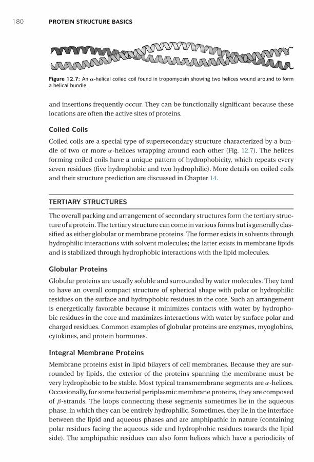
P1: IKB0521840988c12 CB1022/Xiong 0 521 84098 8 January 10, 2006 13:45
180 PROTEIN STRUCTURE BASICS
Figure 12.7: An α-helical coiled coil found in tropomyosin showing two helices wound around to forma helical bundle.
and insertions frequently occur. They can be functionally significant because theselocations are often the active sites of proteins.
Coiled Coils
Coiled coils are a special type of supersecondary structure characterized by a bun-dle of two or more α-helices wrapping around each other (Fig. 12.7). The helicesforming coiled coils have a unique pattern of hydrophobicity, which repeats everyseven residues (five hydrophobic and two hydrophilic). More details on coiled coilsand their structure prediction are discussed in Chapter 14.
TERTIARY STRUCTURES
The overall packing and arrangement of secondary structures form the tertiary struc-ture of a protein. The tertiary structure can come in various forms but is generally clas-sified as either globular or membrane proteins. The former exists in solvents throughhydrophilic interactions with solvent molecules; the latter exists in membrane lipidsand is stabilized through hydrophobic interactions with the lipid molecules.
Globular Proteins
Globular proteins are usually soluble and surrounded by water molecules. They tendto have an overall compact structure of spherical shape with polar or hydrophilicresidues on the surface and hydrophobic residues in the core. Such an arrangementis energetically favorable because it minimizes contacts with water by hydropho-bic residues in the core and maximizes interactions with water by surface polar andcharged residues. Common examples of globular proteins are enzymes, myoglobins,cytokines, and protein hormones.
Integral Membrane Proteins
Membrane proteins exist in lipid bilayers of cell membranes. Because they are sur-rounded by lipids, the exterior of the proteins spanning the membrane must bevery hydrophobic to be stable. Most typical transmembrane segments are α-helices.Occasionally, for some bacterial periplasmic membrane proteins, they are composedof β-strands. The loops connecting these segments sometimes lie in the aqueousphase, in which they can be entirely hydrophilic. Sometimes, they lie in the interfacebetween the lipid and aqueous phases and are amphipathic in nature (containingpolar residues facing the aqueous side and hydrophobic residues towards the lipidside). The amphipathic residues can also form helices which have a periodicity of
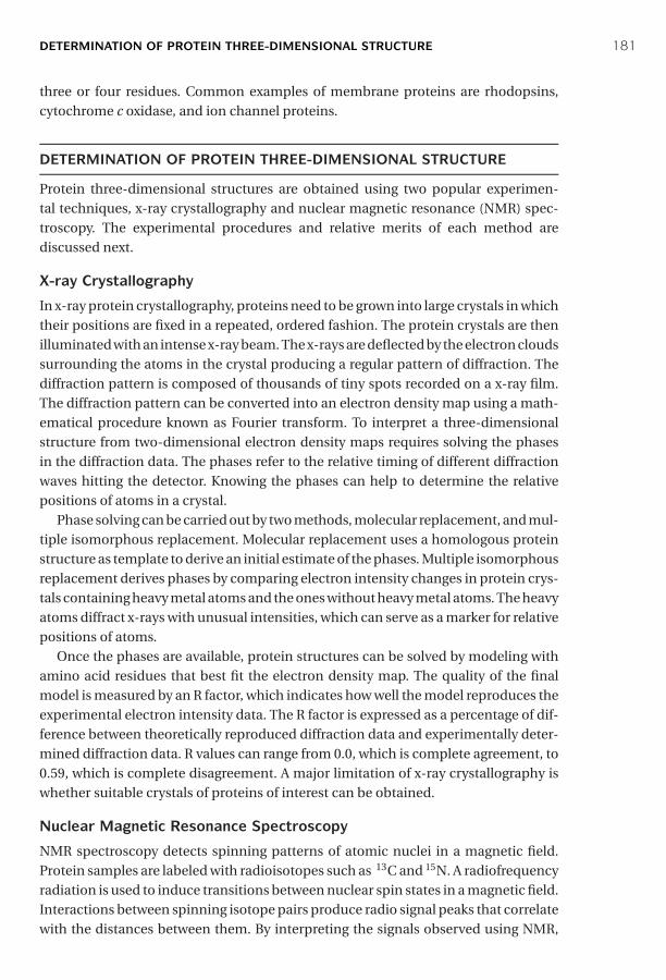
P1: IKB0521840988c12 CB1022/Xiong 0 521 84098 8 January 10, 2006 13:45
DETERMINATION OF PROTEIN THREE-DIMENSIONAL STRUCTURE 181
three or four residues. Common examples of membrane proteins are rhodopsins,cytochrome c oxidase, and ion channel proteins.
DETERMINATION OF PROTEIN THREE-DIMENSIONAL STRUCTURE
Protein three-dimensional structures are obtained using two popular experimen-tal techniques, x-ray crystallography and nuclear magnetic resonance (NMR) spec-troscopy. The experimental procedures and relative merits of each method arediscussed next.
X-ray Crystallography
In x-ray protein crystallography, proteins need to be grown into large crystals in whichtheir positions are fixed in a repeated, ordered fashion. The protein crystals are thenilluminated with an intense x-ray beam. The x-rays are deflected by the electron cloudssurrounding the atoms in the crystal producing a regular pattern of diffraction. Thediffraction pattern is composed of thousands of tiny spots recorded on a x-ray film.The diffraction pattern can be converted into an electron density map using a math-ematical procedure known as Fourier transform. To interpret a three-dimensionalstructure from two-dimensional electron density maps requires solving the phasesin the diffraction data. The phases refer to the relative timing of different diffractionwaves hitting the detector. Knowing the phases can help to determine the relativepositions of atoms in a crystal.
Phase solving can be carried out by two methods, molecular replacement, and mul-tiple isomorphous replacement. Molecular replacement uses a homologous proteinstructure as template to derive an initial estimate of the phases. Multiple isomorphousreplacement derives phases by comparing electron intensity changes in protein crys-tals containing heavy metal atoms and the ones without heavy metal atoms. The heavyatoms diffract x-rays with unusual intensities, which can serve as a marker for relativepositions of atoms.
Once the phases are available, protein structures can be solved by modeling withamino acid residues that best fit the electron density map. The quality of the finalmodel is measured by an R factor, which indicates how well the model reproduces theexperimental electron intensity data. The R factor is expressed as a percentage of dif-ference between theoretically reproduced diffraction data and experimentally deter-mined diffraction data. R values can range from 0.0, which is complete agreement, to0.59, which is complete disagreement. A major limitation of x-ray crystallography iswhether suitable crystals of proteins of interest can be obtained.
Nuclear Magnetic Resonance Spectroscopy
NMR spectroscopy detects spinning patterns of atomic nuclei in a magnetic field.Protein samples are labeled with radioisotopes such as 13C and 15N. A radiofrequencyradiation is used to induce transitions between nuclear spin states in a magnetic field.Interactions between spinning isotope pairs produce radio signal peaks that correlatewith the distances between them. By interpreting the signals observed using NMR,
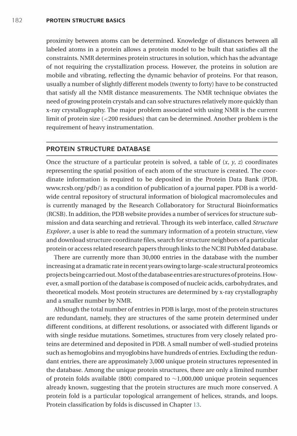
P1: IKB0521840988c12 CB1022/Xiong 0 521 84098 8 January 10, 2006 13:45
182 PROTEIN STRUCTURE BASICS
proximity between atoms can be determined. Knowledge of distances between alllabeled atoms in a protein allows a protein model to be built that satisfies all theconstraints. NMR determines protein structures in solution, which has the advantageof not requiring the crystallization process. However, the proteins in solution aremobile and vibrating, reflecting the dynamic behavior of proteins. For that reason,usually a number of slightly different models (twenty to forty) have to be constructedthat satisfy all the NMR distance measurements. The NMR technique obviates theneed of growing protein crystals and can solve structures relatively more quickly thanx-ray crystallography. The major problem associated with using NMR is the currentlimit of protein size (<200 residues) that can be determined. Another problem is therequirement of heavy instrumentation.
PROTEIN STRUCTURE DATABASE
Once the structure of a particular protein is solved, a table of (x, y, z) coordinatesrepresenting the spatial position of each atom of the structure is created. The coor-dinate information is required to be deposited in the Protein Data Bank (PDB,www.rcsb.org/pdb/) as a condition of publication of a journal paper. PDB is a world-wide central repository of structural information of biological macromolecules andis currently managed by the Research Collaboratory for Structural Bioinformatics(RCSB). In addition, the PDB website provides a number of services for structure sub-mission and data searching and retrieval. Through its web interface, called StructureExplorer, a user is able to read the summary information of a protein structure, viewand download structure coordinate files, search for structure neighbors of a particularprotein or access related research papers through links to the NCBI PubMed database.
There are currently more than 30,000 entries in the database with the numberincreasing at a dramatic rate in recent years owing to large-scale structural proteomicsprojects being carried out. Most of the database entries are structures of proteins. How-ever, a small portion of the database is composed of nucleic acids, carbohydrates, andtheoretical models. Most protein structures are determined by x-ray crystallographyand a smaller number by NMR.
Although the total number of entries in PDB is large, most of the protein structuresare redundant, namely, they are structures of the same protein determined underdifferent conditions, at different resolutions, or associated with different ligands orwith single residue mutations. Sometimes, structures from very closely related pro-teins are determined and deposited in PDB. A small number of well-studied proteinssuch as hemoglobins and myoglobins have hundreds of entries. Excluding the redun-dant entries, there are approximately 3,000 unique protein structures represented inthe database. Among the unique protein structures, there are only a limited numberof protein folds available (800) compared to ∼1,000,000 unique protein sequencesalready known, suggesting that the protein structures are much more conserved. Aprotein fold is a particular topological arrangement of helices, strands, and loops.Protein classification by folds is discussed in Chapter 13.
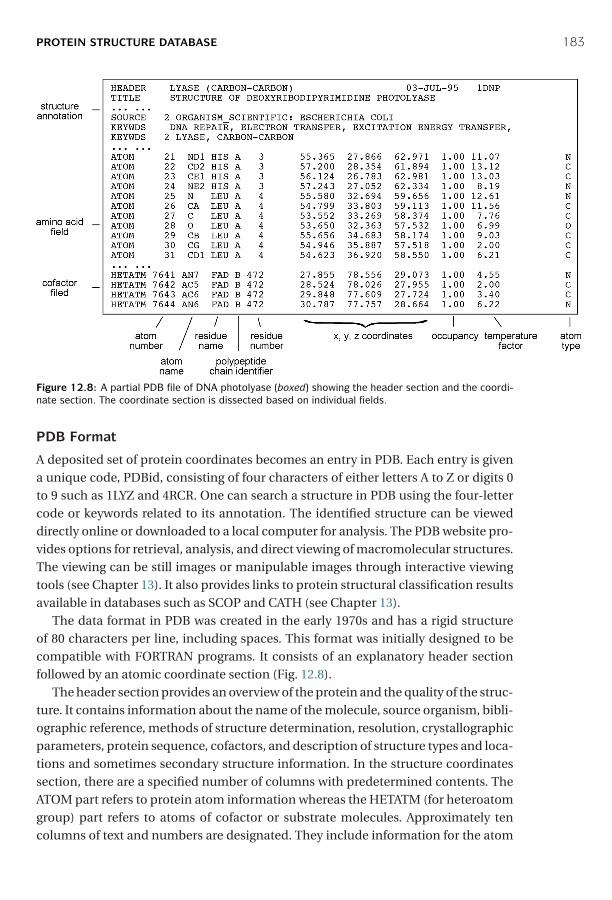
P1: IKB0521840988c12 CB1022/Xiong 0 521 84098 8 January 10, 2006 13:45
PROTEIN STRUCTURE DATABASE 183
Figure 12.8: A partial PDB file of DNA photolyase (boxed) showing the header section and the coordi-nate section. The coordinate section is dissected based on individual fields.
PDB Format
A deposited set of protein coordinates becomes an entry in PDB. Each entry is givena unique code, PDBid, consisting of four characters of either letters A to Z or digits 0to 9 such as 1LYZ and 4RCR. One can search a structure in PDB using the four-lettercode or keywords related to its annotation. The identified structure can be vieweddirectly online or downloaded to a local computer for analysis. The PDB website pro-vides options for retrieval, analysis, and direct viewing of macromolecular structures.The viewing can be still images or manipulable images through interactive viewingtools (see Chapter 13). It also provides links to protein structural classification resultsavailable in databases such as SCOP and CATH (see Chapter 13).
The data format in PDB was created in the early 1970s and has a rigid structureof 80 characters per line, including spaces. This format was initially designed to becompatible with FORTRAN programs. It consists of an explanatory header sectionfollowed by an atomic coordinate section (Fig. 12.8).
The header section provides an overview of the protein and the quality of the struc-ture. It contains information about the name of the molecule, source organism, bibli-ographic reference, methods of structure determination, resolution, crystallographicparameters, protein sequence, cofactors, and description of structure types and loca-tions and sometimes secondary structure information. In the structure coordinatessection, there are a specified number of columns with predetermined contents. TheATOM part refers to protein atom information whereas the HETATM (for heteroatomgroup) part refers to atoms of cofactor or substrate molecules. Approximately tencolumns of text and numbers are designated. They include information for the atom

P1: IKB0521840988c12 CB1022/Xiong 0 521 84098 8 January 10, 2006 13:45
184 PROTEIN STRUCTURE BASICS
number, atom name, residue name, polypeptide chain identifier, residue number, x,y, and z Cartesian coordinates, temperature factor, and occupancy factor. The lasttwo parameters, occupancy and temperature factors, relate to disorders of atomicpositions in crystals.
The PDB format has been in existence for more than three decades. It is fairly easyto read and simple to use. However, the format is not designed for computer extractionof information from the records. Certain restrictions in the format have significantlycomplicated its current use. For instance, in the PDB format, only Cartesian coordi-nates of atoms are given without bonding information. Information such as disulfidebonds has to be interpreted by viewing programs, some of which may fail to do so. Inaddition, the field width for atom number is limited to five characters, meaning thatthe maximum number of atoms per model is 99,999. The field width for polypeptidechains is only one character in width, meaning that no more than 26 chains can beused in a multisubunit protein model. This has made many large protein complexessuch as ribosomes unable to be represented by a single PDB file. They have to bedivided into multiple PDB files.
mmCIF and MMDB Formats
Significant limitations of the PDB format have allowed the development of new for-mats to handle increasingly complicated structure data. The most popular new for-mats include the macromolecular crystallographic information file (mmCIF) and themolecular modeling database (MMDB) file. Both formats are highly parsable by com-puter software, meaning that information in each field of a record can be retrievedseparately. These new formats facilitate the retrieval and organization of informationfrom database structures.
The mmCIF format is similar to the format for a relational database (see Chapter 2)in which a set of tables are used to organize database records. Each table or field ofinformation is explicitly assigned by a tag and linked to other fields through a specialsyntax. An example of an mmCIF containing multiple fields is given below. As shownin Figure 12.9, a single line of description in the header section of PDB is dividedinto many lines or fields with each field having explicit assignment of item namesand item values. Each field starts with an underscore character followed by categoryname and keyword description separated by a period. The annotation in Figure 12.9shows that the data items belong to the category of “struct” or “database.” Followinga keyword tag, a short text string enclosed by quotation marks is used to assign valuesfor the keyword. Using multiple fields with tags for the same information has theadvantage of providing an explicit reference to each item in a data file and ensures aone-to-one relationship between item names and item values. By presenting the dataitem by item, the format provides much more flexibility for information storage andretrieval.
Another new format is the MMDB format developed by the NCBI to parse andsort pieces of information in PDB. The objective is to allow the information to bemore easily integrated with GenBank and Medline through Entrez (see Chapter 2).
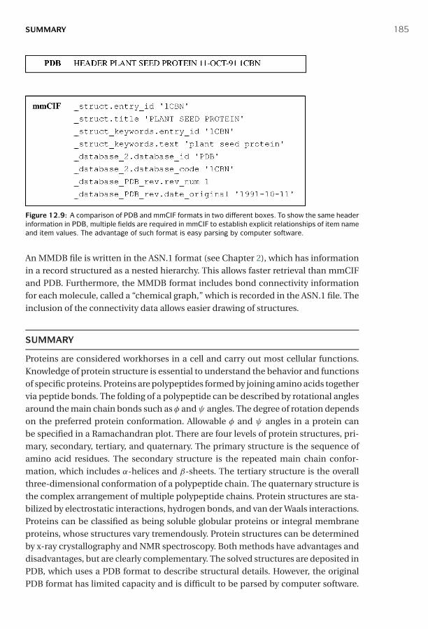
P1: IKB0521840988c12 CB1022/Xiong 0 521 84098 8 January 10, 2006 13:45
SUMMARY 185
Figure 12.9: A comparison of PDB and mmCIF formats in two different boxes. To show the same headerinformation in PDB, multiple fields are required in mmCIF to establish explicit relationships of item nameand item values. The advantage of such format is easy parsing by computer software.
An MMDB file is written in the ASN.1 format (see Chapter 2), which has informationin a record structured as a nested hierarchy. This allows faster retrieval than mmCIFand PDB. Furthermore, the MMDB format includes bond connectivity informationfor each molecule, called a “chemical graph,” which is recorded in the ASN.1 file. Theinclusion of the connectivity data allows easier drawing of structures.
SUMMARY
Proteins are considered workhorses in a cell and carry out most cellular functions.Knowledge of protein structure is essential to understand the behavior and functionsof specific proteins. Proteins are polypeptides formed by joining amino acids togethervia peptide bonds. The folding of a polypeptide can be described by rotational anglesaround the main chain bonds such as φ and ψ angles. The degree of rotation dependson the preferred protein conformation. Allowable φ and ψ angles in a protein canbe specified in a Ramachandran plot. There are four levels of protein structures, pri-mary, secondary, tertiary, and quaternary. The primary structure is the sequence ofamino acid residues. The secondary structure is the repeated main chain confor-mation, which includes α-helices and β-sheets. The tertiary structure is the overallthree-dimensional conformation of a polypeptide chain. The quaternary structure isthe complex arrangement of multiple polypeptide chains. Protein structures are sta-bilized by electrostatic interactions, hydrogen bonds, and van der Waals interactions.Proteins can be classified as being soluble globular proteins or integral membraneproteins, whose structures vary tremendously. Protein structures can be determinedby x-ray crystallography and NMR spectroscopy. Both methods have advantages anddisadvantages, but are clearly complementary. The solved structures are deposited inPDB, which uses a PDB format to describe structural details. However, the originalPDB format has limited capacity and is difficult to be parsed by computer software.

P1: IKB0521840988c12 CB1022/Xiong 0 521 84098 8 January 10, 2006 13:45
186 PROTEIN STRUCTURE BASICS
To overcome the limitations, new formats such as mmCIF and MMDB have beendeveloped.
FURTHER READING
Branden, C., and Tooze, J. 1999. Introduction to Protein Structure, 2nd ed. New York: GarlandPublishing.
Scheeff, E. D., and Fink, J. L. 2003. “Fundamentals of protein structure.” In Structural Bio-informatics, edited by P. E. Bourne and H. Weissig, 15–39. Hoboken, NJ: Wiley-Liss.
Westbrook, J. D., and Fitzgerald, P. M. D. 2003. “The PDB format, mmCIF and other dataformats.” In Structural Bioinformatics, edited by P. E. Bourne and H. Weissig, 161–79.Hoboken, NJ: Wiley-Liss.
P1: JZP0521840988c13 CB1022/Xiong 0 521 84098 8 January 10, 2006 13:50
CHAPTER THIRTEEN
Protein Structure Visualization, Comparison,and Classification
Once a protein structure has been solved, the structure has to be presented in a three-dimensional view on the basis of the solved Cartesian coordinates. Before computervisualization software was developed, molecular structures were represented by phys-ical models of metal wires, rods, and spheres. With the development of computer hard-ware and software technology, sophisticated computer graphics programs have beendeveloped for visualizing and manipulating complicated three-dimensional struc-tures. The computer graphics help to analyze and compare protein structures to gaininsight to functions of the proteins.
PROTEIN STRUCTURAL VISUALIZATION
The main feature of computer visualization programs is interactivity, which allowsusers to visually manipulate the structural images through a graphical user interface.At the touch of a mouse button, a user can move, rotate, and zoom an atomic modelon a computer screen in real time, or examine any portion of the structure in greatdetail, as well as draw it in various forms in different colors. Further manipulations caninclude changing the conformation of a structure by protein modeling or matching aligand to an enzyme active site through docking exercises.
Because a Protein Data Bank (PDB) data file for a protein structure contains onlyx, y, and z coordinates of atoms (see Chapter 12), the most basic requirement fora visualization program is to build connectivity between atoms to make a view ofa molecule. The visualization program should also be able to produce molecularstructures in different styles, which include wire frames, balls and sticks, space-fillingspheres, and ribbons (Fig. 13.1).
A wire-frame diagram is a line drawing representing bonds between atoms. Thewire frame is the simplest form of model representation and is useful for localizingpositions of specific residues in a protein structure, or for displaying a skeletal formof a structure when Cα atoms of each residue are connected. Balls and sticks are solidspheres and rods, representing atoms and bonds, respectively. These diagrams canalso be used to represent the backbone of a structure. In a space-filling representation(or Corey, Pauling, and Koltan [CPK]), each atom is described using large solid sphereswith radii corresponding to the van der Waals radii of the atoms. Ribbon diagramsuse cylinders or spiral ribbons to represent α-helices and broad, flat arrows to rep-resent β-strands. This type of representation is very attractive in that it allows easy
187

P1: JZP0521840988c13 CB1022/Xiong 0 521 84098 8 January 10, 2006 13:50
188 PROTEIN STRUCTURE VISUALIZATION, COMPARISON, AND CLASSIFICATION
Figure 13.1: Examples of molecular structure visualization forms. (A) Wireframes. (B) Balls and sticks.(C) Space-filling spheres. (D) Ribbons (see color plate section).
identification of secondary structure elements and gives a clear view of the overalltopology of the structure. The resulting images are also visually appealing.
Different representation styles can be used in combination to highlight a certainfeature of a structure while deemphasizing the structures surrounding it. For exam-ple, a cofactor of an enzyme can be shown as space-filling spheres while the restof the protein structure is shown as wire frames or ribbons. Some widely used andfreely available software programs for molecular graphics are introduced next withexamples of rendering provided in Figure 13.2.
RasMol (http://rutgers.rcsb.org/pdb/help-graphics.html#rasmol download) is acommand-line–based viewing program that calculates connectivity of a coordinatefile and displays wireframe, cylinder, stick bonds, α-carbon trace, space-filling (CPK)spheres, and ribbons. It reads both PDB and mmCIF formats and can display awhole molecule or specific parts of it. It is available in multiple platforms: UNIX,Windows, and Mac. RasTop (www.geneinfinity.org/rastop/) is a new version of RasMolfor Windows with a more enhanced user interface.
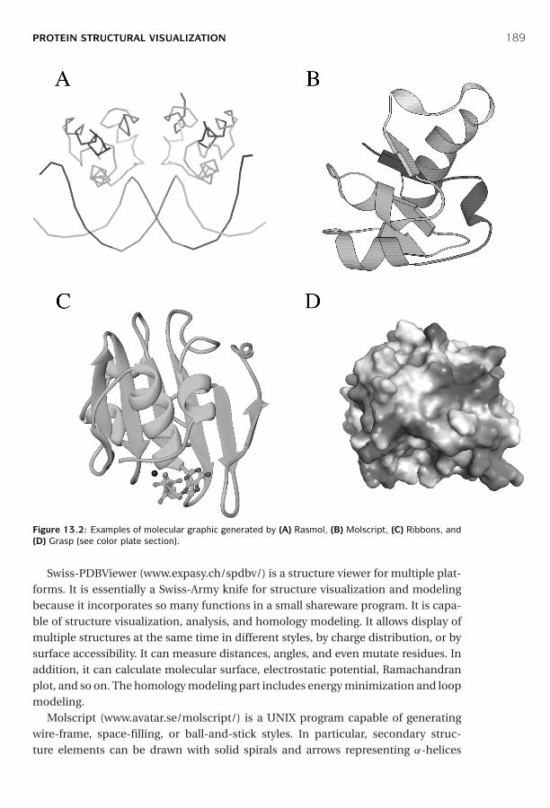
P1: JZP0521840988c13 CB1022/Xiong 0 521 84098 8 January 10, 2006 13:50
PROTEIN STRUCTURAL VISUALIZATION 189
Figure 13.2: Examples of molecular graphic generated by (A) Rasmol, (B) Molscript, (C) Ribbons, and(D) Grasp (see color plate section).
Swiss-PDBViewer (www.expasy.ch/spdbv/) is a structure viewer for multiple plat-forms. It is essentially a Swiss-Army knife for structure visualization and modelingbecause it incorporates so many functions in a small shareware program. It is capa-ble of structure visualization, analysis, and homology modeling. It allows display ofmultiple structures at the same time in different styles, by charge distribution, or bysurface accessibility. It can measure distances, angles, and even mutate residues. Inaddition, it can calculate molecular surface, electrostatic potential, Ramachandranplot, and so on. The homology modeling part includes energy minimization and loopmodeling.
Molscript (www.avatar.se/molscript/) is a UNIX program capable of generatingwire-frame, space-filling, or ball-and-stick styles. In particular, secondary struc-ture elements can be drawn with solid spirals and arrows representing α-helices

P1: JZP0521840988c13 CB1022/Xiong 0 521 84098 8 January 10, 2006 13:50
190 PROTEIN STRUCTURE VISUALIZATION, COMPARISON, AND CLASSIFICATION
and β-strands, respectively. Visually appealing images can be generated that are ofpublication quality. The drawback is that the program is command-line–based andnot very user friendly. A modified UNIX program called Bobscript (www.strubi.ox.ac.uk/bobscript/) is available with enhanced features.
Ribbons (http://sgce.cbse.uab.edu/ribbons/) another UNIX program similar toMolscript, generates ribbon diagrams depicting protein secondary structures. Aesthe-tically appealing images can be produced that are of publication quality. However, theprogram, which is also command-line-based, is extremely difficult to use.
Grasp (http://trantor.bioc.columbia.edu/grasp/) is a UNIX program that gener-ates solid molecular surface images and uses a gradated coloring scheme to displayelectrostatic charges on the surface.
There are also a number of web-based visualization tools that use Java applets.These programs tend to have limited molecular display features and low-qualityimages. However, the advantage is that the user does not have to download, compile,and install the programs locally, but simply view the structures on a web browserusing any kind of computer operating system. In fact, the PDB also attempts tosimplify the database structure display for end users. It has incorporated a num-ber of light-weight Java-based structure viewers in the PDB web site (see Chap-ter 12).
WebMol (www.cmpharm.ucsf.edu/cgi-bin/webmol.pl) is a web-based programbuilt based on a modified RasMol code and thus shares many similarities with RasMol.It runs directly on a browser of any type as an applet and is able to display simple linedrawing models of protein structures. It also has a feature of interactively displayingRamachandran plots for structure model evaluation.
Chime (www.mdlchime.com/chime/) is a plug-in for web browsers; it is not a stand-alone program and has to be invoked in a web browser. The program is also derivedfrom RasMol and allows interactive display of graphics of protein structures inside aweb browser.
Cn3D (www.ncbi.nlm.nih.gov/Structure/CN3D/cn3d.shtml) is a helper applica-tion for web browsers to display structures in the MMDB format from the NCBI’sstructural database. It can be used on- or offline as a stand-alone program. It is ableto render three-dimensional molecular models and display secondary structure car-toons. The drawback is that it does not recognize the PDB format.
PROTEIN STRUCTURE COMPARISON
With the visualization and computer graphics tools available, it becomes easy toobserve and compare protein structures. To compare protein structures is to ana-lyze two or more protein structures for similarity. The comparative analysis often,but not always, involves the direct alignment and superimposition of structures ina three-dimensional space to reveal which part of structure is conserved and whichpart is different at the three-dimensional level.
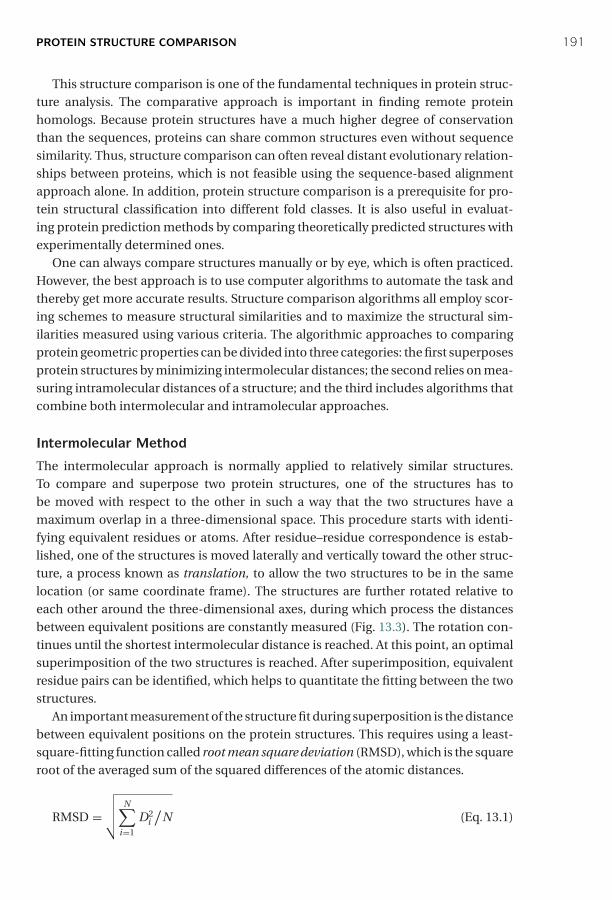
P1: JZP0521840988c13 CB1022/Xiong 0 521 84098 8 January 10, 2006 13:50
PROTEIN STRUCTURE COMPARISON 191
This structure comparison is one of the fundamental techniques in protein struc-ture analysis. The comparative approach is important in finding remote proteinhomologs. Because protein structures have a much higher degree of conservationthan the sequences, proteins can share common structures even without sequencesimilarity. Thus, structure comparison can often reveal distant evolutionary relation-ships between proteins, which is not feasible using the sequence-based alignmentapproach alone. In addition, protein structure comparison is a prerequisite for pro-tein structural classification into different fold classes. It is also useful in evaluat-ing protein prediction methods by comparing theoretically predicted structures withexperimentally determined ones.
One can always compare structures manually or by eye, which is often practiced.However, the best approach is to use computer algorithms to automate the task andthereby get more accurate results. Structure comparison algorithms all employ scor-ing schemes to measure structural similarities and to maximize the structural sim-ilarities measured using various criteria. The algorithmic approaches to comparingprotein geometric properties can be divided into three categories: the first superposesprotein structures by minimizing intermolecular distances; the second relies on mea-suring intramolecular distances of a structure; and the third includes algorithms thatcombine both intermolecular and intramolecular approaches.
Intermolecular Method
The intermolecular approach is normally applied to relatively similar structures.To compare and superpose two protein structures, one of the structures has tobe moved with respect to the other in such a way that the two structures have amaximum overlap in a three-dimensional space. This procedure starts with identi-fying equivalent residues or atoms. After residue–residue correspondence is estab-lished, one of the structures is moved laterally and vertically toward the other struc-ture, a process known as translation, to allow the two structures to be in the samelocation (or same coordinate frame). The structures are further rotated relative toeach other around the three-dimensional axes, during which process the distancesbetween equivalent positions are constantly measured (Fig. 13.3). The rotation con-tinues until the shortest intermolecular distance is reached. At this point, an optimalsuperimposition of the two structures is reached. After superimposition, equivalentresidue pairs can be identified, which helps to quantitate the fitting between the twostructures.
An important measurement of the structure fit during superposition is the distancebetween equivalent positions on the protein structures. This requires using a least-square-fitting function called root mean square deviation (RMSD), which is the squareroot of the averaged sum of the squared differences of the atomic distances.
RMSD =√√√√ N∑
i=1
D2i
/N (Eq. 13.1)
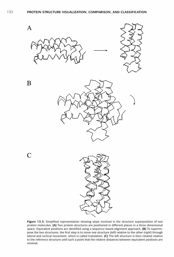
P1: JZP0521840988c13 CB1022/Xiong 0 521 84098 8 January 10, 2006 13:50
192 PROTEIN STRUCTURE VISUALIZATION, COMPARISON, AND CLASSIFICATION
Figure 13.3: Simplified representation showing steps involved in the structure superposition of twoprotein molecules. (A) Two protein structures are positioned in different places in a three dimensionalspace. Equivalent positions are identified using a sequence based alignment approach. (B) To superim-pose the two structures, the first step is to move one structure (left) relative to the other (right) throughlateral and vertical movement, which is called translation. (C) The left structure is then rotated relativeto the reference structure until such a point that the relative distances between equivalent positions areminimal.
P1: JZP0521840988c13 CB1022/Xiong 0 521 84098 8 January 10, 2006 13:50
PROTEIN STRUCTURE COMPARISON 193
where D is the distance between coordinate data points and N is the total number ofcorresponding residue pairs.
In practice, only the distances between Cα carbons of corresponding residues aremeasured. The goal of structural comparison is to achieve a minimum RMSD. How-ever, the problem with RMSD is that it depends on the size of the proteins being com-pared. For the same degree of sequence identity, large proteins tend to have higherRMSD values than small proteins when an optimal alignment is reached. Recently, alogarithmic factor has been proposed to correct this size-dependency problem. Thisnew measure is called RMSD100 and is determined by the following formula:
RMSD100 = RMSD−1.3 + 0.5 ln(N)
(Eq. 13.2)
where N is the total number of corresponding atoms.Although this corrected RMSD is more reliable than the raw RMSD for structure
superposition, a low RMSD value by no means guarantees a correct alignment oran alignment with biological meaning. Careful scrutiny of the automatic alignmentresults is always recommended.
The most challenging part of using the intermolecular method is to identify equiv-alent residues in the first place, which often resorts to sequence alignment meth-ods. Obviously, this restricts the usefulness of structural comparison between distanthomologs.
A number of solutions have been proposed to compare more distantly related struc-tures. One approach that has been proposed is to delete sequence variable regionsoutside secondary structure elements to reduce the search time required to find anoptimum superposition. However, this method does not guarantee an optimal align-ment. Another approach adopted by some researchers is to divide the proteins intosmall fragments (e.g., every six to nine residues). Matching of similar regions at thethree-dimensional level is then done fragment by fragment. After finding the best fit-ting fragments, a joint superposition for the entire structure is performed. The thirdapproach is termed iterative optimization, during which the two sequences are firstaligned using dynamic programming. Identified equivalent residues are used to guidea first round of superposition. After superposition, more residues are identified to be inclose proximity at the three-dimensional level and considered as equivalent residues.Based on the newly identified equivalent residues, a new round of superposition isgenerated to refine from the previous alignment. This procedure is repeated until theRMSD values cannot be further improved.
Intramolecular Method
The intramolecular approach relies on structural internal statistics and therefore doesnot depend on sequence similarity between the proteins to be compared. In addition,this method does not generate a physical superposition of structures, but insteadprovides a quantitative evaluation of the structural similarity between correspondingresidue pairs.

P1: JZP0521840988c13 CB1022/Xiong 0 521 84098 8 January 10, 2006 13:50
194 PROTEIN STRUCTURE VISUALIZATION, COMPARISON, AND CLASSIFICATION
The method works by generating a distance matrix between residues of the sameprotein. In comparing two protein structures, the distance matrices from the twostructures are moved relative to each other to achieve maximum overlaps. By over-laying two distance matrices, similar intramolecular distance patterns representingsimilar structure folding regions can be identified. For the ease of comparison, eachmatrix is decomposed into smaller submatrices consisting of hexapeptide fragments.To maximize the similarity regions between two structures, a Monte Carlo procedureis used. By reducing three-dimensional information into two-dimensional informa-tion, this strategy identifies overall structural resemblances and common structurecores.
Combined Method
A recent development in structure comparison involves combining both inter- andintramolecular approaches. In the hybrid approach, corresponding residues can beidentified using the intramolecular method. Subsequent structure superposition canbe performed based on residue equivalent relationships. In addition to using RMSDas a measure during alignment, additional structural properties such as secondarystructure types, torsion angles, accessibility, and local hydrogen bonding environmentcan be used. Dynamic programming is often employed to maximize overlaps in bothinter- and intramolecular comparisons.
Multiple Structure Alignment
In addition to pairwise alignment, a number of algorithms can also perform mul-tiple structure alignment. The alignment strategy is similar to the Clustal sequencealignment using a progressive approach (see Chapter 5). That is, all structures are firstcompared in a pairwise fashion. A distance matrix is developed based on structuresimilarity scores such as RMSD. This allows construction of a phylogenetic tree, whichguides the subsequent clustering of the structures. The most similar two structuresare then realigned. The aligned structures create a median structure that allows otherstructures to be progressively added for comparison based on the hierarchy describedin the guide tree. When all the structures in the set are added, this eventually creates amultiple structure alignment. Several popular on-line structure comparison resourcesare discussed next.
DALI (www2.ebi.ac.uk/dali/) is a structure comparison web server that uses theintramolecular distance method. It works by maximizing the similarity of two distancegraphs. The matrices are based on distances between all Cα atoms for each individualprotein. Two distance matrices are overlaid and moved one relative to the other toidentify most similar regions. DALI uses a statistical significance value called a Z-scoreto evaluate structural alignment. The Z-score is the number of standard deviationsfrom the average score derived from the database background distribution. The higherthe Z-score when comparing a pair of protein structures, the less likely the similarity

P1: JZP0521840988c13 CB1022/Xiong 0 521 84098 8 January 10, 2006 13:50
PROTEIN STRUCTURE CLASSIFICATION 195
observed is a result of random chance. Empirically, a Z-score >4 indicates a significantlevel of structure similarity. The web server is at the same time a database that containsZ-scores of all precomputed structure pairs of proteins in PDB. The user can upload astructure to compare it with all known structures, or perform a pairwise comparisonof two uploaded structures.
CE (Combinatorial Extension; http://cl.sdsc.edu/ce.html) is a web-based programthat also uses the intramolecular distance approach. However, unlike DALI, a type ofheuristics is used. In this method, every eight residues are treated as a single residue.The Cα distance matrices are constructed at the level of octameric “residues.” Inthis way, the computational time required to search for the best alignment is con-siderably reduced, at the expense of alignment accuracy. CE also uses a Z-scoreas a measure of significance of an alignment. A Z-score >3.5 indicates a similarfold.
VAST (Vector Alignment Search Tool; www.ncbi.nlm.nih.gov:80/Structure/VAST/vast.shtml) is a web server that performs alignment using both the inter- andintramolecular approaches. The superposition is based on information of direction-ality of secondary structural elements (represented as vectors). Optimal alignmentbetween two structures is defined by the highest degree of vector matches.
SSAP (www.biochem.ucl.ac.uk/cgi-bin/cath/GetSsapRasmol.pl) is a web serverthat uses an intramolecular distance–based method in which matrices are built basedon the Cβ distances of all residue pairs. When comparing two different matrices, adynamic programming approach is used to find the path of residue positions withoptimal scores. The dynamic programming is applied at two levels, one at a lowerlevel in which all residue pairs between the proteins are compared and another at anupper level in which subsequently identified equivalent residue pairs are processedto refine the matching positions. This process is known as double dynamic program-ming. An SSAP score is reported for structural similarity. A score above 70 indicates agood structural similarity.
STAMP (www.compbio.dundee.ac.uk/Software/Stamp/stamp.html) is a UNIX pro-gram that uses the intermolecular approach to generate protein structure alignment.The main feature is the use of iterative alignment based on dynamic programming toobtain the best superposition of two or more structures.
PROTEIN STRUCTURE CLASSIFICATION
One of the applications of protein structure comparison is structural classification.The ability to compare protein structures allows classification of the structure dataand identification of relationships among structures. The reason to develop a pro-tein structure classification system is to establish hierarchical relationships amongprotein structures and to provide a comprehensive and evolutionary view of knownstructures. Once a hierarchical classification system is established, a newly obtainedprotein structure can find its place in a proper category. As a result, its functionscan be better understood based on association with other proteins. To date, several

P1: JZP0521840988c13 CB1022/Xiong 0 521 84098 8 January 10, 2006 13:50
196 PROTEIN STRUCTURE VISUALIZATION, COMPARISON, AND CLASSIFICATION
systems have been developed, the two most popular being Structural Classifica-tion of Proteins (SCOP) and Class, Architecture, Topology and Homologous (CATH).The following introduces the basic steps in establishing the systems to classifyproteins.
The first step in structure classification is to remove redundancy from databases.As mentioned in Chapter 12, among the tens of thousands of entries in PDB, themajority of the structures are redundant as they correspond to structures solvedat different resolutions, or associated with different ligands or with single-residuemutations. The redundancy can be removed by selecting representatives througha sequence alignment–based approach. The second step is to separate structurallydistinct domains within a structure. Because some proteins are composed of mul-tiple domains, they must be subdivided before a sensible structural comparisoncan be carried out. This domain identification and separation can be done eithermanually or based on special algorithms for domain recognition. Once multidomainproteins are split into separate domains, structure comparison can be conducted atthe domain level, either through manual inspection, or automated structural align-ment, or a combination of both. The last step involves grouping proteins/domainsof similar structures and clustering them based on different levels of resemblancein secondary structure composition and arrangement of the secondary structures inspace.
As mentioned, the two most popular classification schemes are SCOP and CATH,both of which contain a number of hierarchical levels in their systems.
SCOP
SCOP (http://scop.mrc-lmb.cam.ac.uk/scop/) is a database for comparing and clas-sifying protein structures. It is constructed almost entirely based on manual exam-ination of protein structures. The proteins are grouped into hierarchies of classes,folds, superfamilies, and families. In the latest SCOP release version (v1.65, releasedDecember 2003), there are 7 classes, 800 folds, 1,294 superfamilies, and 2,327 families.
The SCOP families consist of proteins having high sequence identity (>30%).Thus, the proteins within a family clearly share close evolutionary relationships andnormally have the same functionality. The protein structures at this level are alsoextremely similar. Superfamilies consist of families with similar structures, but weaksequence similarity. It is believed that members of the same superfamily share a com-mon ancestral origin, although the relationships between families are considereddistant. Folds consist of superfamilies with a common core structure, which is deter-mined manually. This level describes similar overall secondary structures with similarorientation and connectivity between them. Members within the same fold do notalways have evolutionary relationships. Some of the shared core structure may be aresult of analogy. Classes consist of folds with similar core structures. This is at thehighest level of the hierarchy, which distinguishes groups of proteins by secondarystructure compositions such as all α, all β, α and β, and so on. Some classes are cre-ated based on general features such as membrane proteins, small proteins with few

P1: JZP0521840988c13 CB1022/Xiong 0 521 84098 8 January 10, 2006 13:50
PROTEIN STRUCTURE CLASSIFICATION 197
secondary structures and irregular proteins. Folds within the same class are essentiallyrandomly related in evolution.
CATH
CATH (www.biochem.ucl.ac.uk/bsm/cath new/index.html) classifies proteins basedon the automatic structural alignment program SSAP as well as manual comparison.Structural domain separation is carried out also as a combined effort of a humanexpert and computer programs. Individual domain structures are classified at fivemajor levels: class, architecture, fold/topology, homologous superfamily, and homol-ogous family. In the CATH release version 2.5.1 (January 2004), there are 4 classes,37 architectures, 813 topologies, 1,467 homologous superfamilies, and 4,036 homol-ogous families.
The definition for class in CATH is similar to that in SCOP, and is based on secondarystructure content. Architecture is a unique level in CATH, intermediate between foldand class. This level describes the overall packing and arrangement of secondarystructures independent of connectivity between the elements. The topology level isequivalent to the fold level in SCOP, which describes overall orientation of secondarystructures and takes into account the sequence connectivity between the secondarystructure elements. The homologous superfamily and homologous family levels areequivalent to the superfamily and family levels in SCOP with similar evolutionarydefinitions, respectively.
Comparison of SCOP and CATH
SCOP is almost entirely based on manual comparison of structures by human expertswith no quantitative criteria to group proteins. It is argued that this approach offerssome flexibility in recognizing distant structural relatives, because human brainsmay be more adept at recognizing slightly dissimilar structures that essentially havethe same architecture. However, this reliance on human expertise also renders themethod subjective. The exact boundaries between levels and groups are sometimesarbitrary.
CATH is a combination of manual curation and automated procedure, which makesthe process less subjective. For example, in defining domains, CATH first relies on theconsensus of three different algorithms to recognize domains. When the computerprograms disagree, human intervention will take place. In addition, the extra Architec-ture level in CATH makes the structure classification more continuous. The drawbackof the systems is that the fixed thresholds in structural comparison may make assign-ment less accurate.
Due to the differences in classification criteria, one might expect that there wouldbe huge differences in classification results. In fact, the classification results fromboth systems are quite similar. Exhaustive analysis has shown that the results fromthe two systems converge at about 80% of the time. In other words, only about 20%of the structure fold assignments are different. Figure 13.4 shows two examples ofagreement and disagreement based on classification by the two systems.
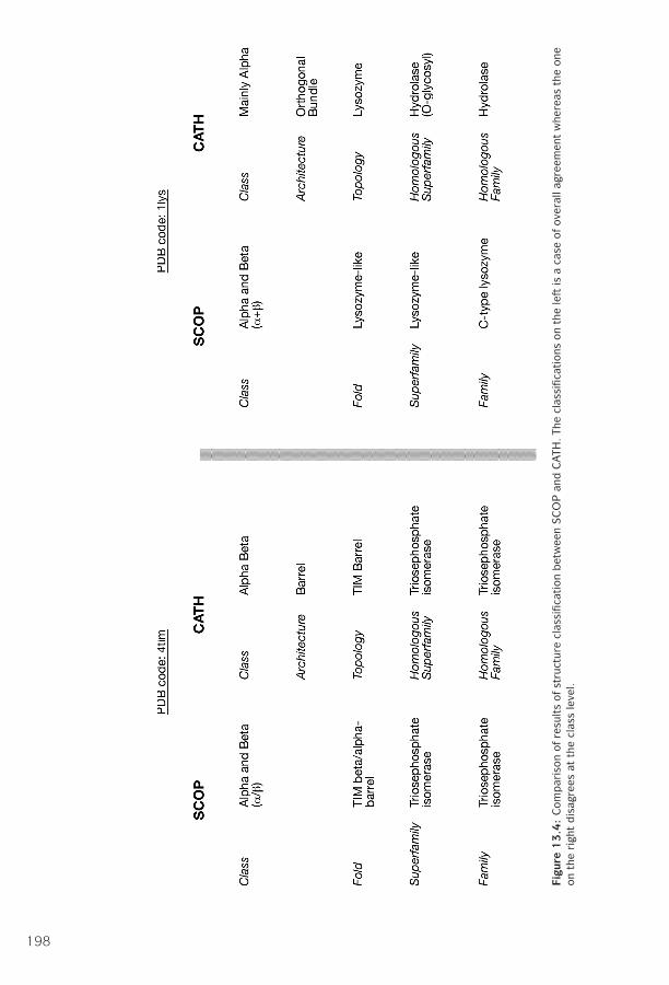
P1: JZP0521840988c13 CB1022/Xiong 0 521 84098 8 January 10, 2006 13:50
Figu
re1
3.4
:C
ompar
ison
ofre
sults
ofst
ruct
ure
clas
sific
atio
nbet
wee
nSC
OP
and
CATH
.Th
ecl
assi
ficat
ions
onth
ele
ftis
aca
seof
over
alla
gree
men
tw
here
asth
eon
eon
the
righ
tdis
agre
esat
the
clas
sle
vel.
198

P1: JZP0521840988c13 CB1022/Xiong 0 521 84098 8 January 10, 2006 13:50
FURTHER READING 199
SUMMARY
A clear and concise visual representation of protein structures is the first step towardsstructural understanding. A number of visualization programs have been developedfor that purpose. They include stand-alone programs for sophisticated manipulationof structures and light-weight web-based programs for simple structure viewing. Pro-tein structure comparison allows recognition of distant evolutionary relationshipsamong proteins and is helpful for structure classification and evaluation of proteinstructure prediction methods. The comparison algorithms fall into three categories:the intermolecular method, which involves transformation of atomic coordinates ofstructures to get optimal superimposition; the intramolecular method, which con-structs an inter-residue distance matrix within a molecule and compares the matrixagainst that from a second molecule; and the combined method that uses bothinter- and intramolecular approaches. Among all the structure comparison algo-rithms developed so far, DALI is most widely used. Protein structure classificationis important for understanding protein structure, function and evolution. The mostwidely used classification schemes are SCOP and CATH. The two systems largelyagree but differ somewhat. Each system has its own strengths and neither appears tobe superior. It is thus advisable to compare the classification results from both systemsin order to put a structure in the correct context.
FURTHER READING
Bourne, P. E., and Shindyalov, I. N. 2003. “Structure comparison and alignment.” In StructuralBioinformatics, edited by P. E. Bourne and H. Weissig, 321–37. Hoboken, NJ: Wiley-Liss.
Carugo, O., and Pongor, S. 2002. Recent progress in protein 3D structure comparison. Curr.Protein Pept. Sci. 3:441–9.
Hadley, C., and Jones, D. T. 1999. A systematic comparison of protein structure classifications:SCOP, CATH, and FSSP. Structure 7:1099–112.
Jawad, Z., and Paoli, M. 2002. Novel sequences propel familiar folds. Structure 10:447–54.Kinch, L. N., and Grishin, N. V. 2002. Evolution of protein structures and functions. Curr. Opin.
Struct. Biol. 12:400–8.Koehl, P. 2001. Protein structure similarities. Curr. Opin. Struct. Biol. 11:348–53.Orengo, C. A., Pearl, F. M. G., and Thornton, J. M. 2003. “The CATH domain structure database.”
In Structural Bioinformatics, edited by P. E. Bourne and H. Weissig, 249–71. Hoboken, NJ:Wiley-Liss.
Ouzounis, C. A., Coulson, R. M., Enright, A. J., Kunin, V., and Pereira-Leal, J. B. 2003. Classifica-tion schemes for protein structure and function. Nat. Rev. Genet. 4:508–19.
Reddy, B. J. 2003. “Protein structure evolution and the scop database.” In Structural Bioinfor-matics, edited by P. E. Bourne and H. Weissig, 239–48. Hoboken, NJ: Wiley-Liss.
Russell, R. B. 2002. Classification of protein folds. Mol. Biotechnol. 20:17–28.Tate, J. 2003. “Molecular visualization.” In Structural Bioinformatics, edited by P. E. Bourne and
H. Weissig, 135–58. Hoboken, NJ: Wiley-Liss.
P1: JZP0521840988c14 CB1022/Xiong 0 521 84098 8 January 10, 2006 15:14
CHAPTER FOURTEEN
Protein Secondary Structure Prediction
Protein secondary structures are stable local conformations of a polypeptide chain.They are critically important in maintaining a protein three-dimensional structure.The highly regular and repeated structural elements include α-helices and β-sheets.It has been estimated that nearly 50% of residues of a protein fold into either α-helicesand β-strands. As a review, an α-helix is a spiral-like structure with 3.6 amino acidresidues per turn. The structure is stabilized by hydrogen bonds between residues iand i + 4. Prolines normally do not occur in the middle of helical segments, but can befound at the end positions of α-helices (see Chapter 12). A β-sheet consists of two ormore β-strands having an extended zigzag conformation. The structure is stabilizedby hydrogen bonding between residues of adjacent strands, which actually may belong-range interactions at the primary structure level. β-Strands at the protein surfaceshow an alternating pattern of hydrophobic and hydrophilic residues; buried strandstend to contain mainly hydrophobic residues.
Protein secondary structure prediction refers to the prediction of the conforma-tional state of each amino acid residue of a protein sequence as one of the threepossible states, namely, helices, strands, or coils, denoted as H, E, and C, respec-tively. The prediction is based on the fact that secondary structures have a regulararrangement of amino acids, stabilized by hydrogen bonding patterns. The structuralregularity serves the foundation for prediction algorithms.
Predicting protein secondary structures has a number of applications. It can beuseful for the classification of proteins and for the separation of protein domains andfunctional motifs. Secondary structures are much more conserved than sequencesduring evolution. As a result, correctly identifying secondary structure elements(SSE) can help to guide sequence alignment or improve existing sequence align-ment of distantly related sequences. In addition, secondary structure predictionis an intermediate step in tertiary structure prediction as in threading analysis(see Chapter 15).
Because of significant structural differences between globular proteins and trans-membrane proteins, they necessitate very different approaches to predicting respec-tive secondary structure elements. Prediction methods for each of two types of pro-teins are discussed herein. In addition, prediction of supersecondary structures, suchas coiled coils, is also described.
200
P1: JZP0521840988c14 CB1022/Xiong 0 521 84098 8 January 10, 2006 15:14
SECONDARY STRUCTURE PREDICTION FOR GLOBULAR PROTEINS 201
SECONDARY STRUCTURE PREDICTION FOR GLOBULAR PROTEINS
Protein secondary structure prediction with high accuracy is not a trivial ask. Itremained a very difficult problem for decades. This is because protein secondarystructure elements are context dependent. The formation of α-helices is determinedby short-range interactions, whereas the formation of β-strands is strongly influencedby long-range interactions. Prediction for long-range interactions is theoretically dif-ficult. After more than three decades of effort, prediction accuracies have only beenimproved from about 50% to about 75%.
The secondary structure prediction methods can be either ab initio based, whichmake use of single sequence information only, or homology based, which make useof multiple sequence alignment information. The ab initio methods, which belongto early generation methods, predict secondary structures based on statistical cal-culations of the residues of a single query sequence. The homology-based methodsdo not rely on statistics of residues of a single sequence, but on common secondarystructural patterns conserved among multiple homologous sequences.
Ab Initio–Based Methods
This type of method predicts the secondary structure based on a single querysequence. It measures the relative propensity of each amino acid belonging to acertain secondary structure element. The propensity scores are derived from knowncrystal structures. Examples of ab initio prediction are the Chou–Fasman and Garnier,Osguthorpe, Robson (GOR) methods. The ab initio methods were developed in the1970s when protein structural data were very limited. The statistics derived from thelimited data sets can therefore be rather inaccurate. However, the methods are sim-ple enough that they are often used to illustrate the basics of secondary structureprediction.
The Chou–Fasman algorithm (http://fasta.bioch.virginia.edu/fasta/chofas.htm)determines the propensity or intrinsic tendency of each residue to be in the helix,strand, and β-turn conformation using observed frequencies found in protein crys-tal structures (conformational values for coils are not considered). For example, it isknown that alanine, glutamic acid, and methionine are commonly found in α-helices,whereas glycine and proline are much less likely to be found in such structures.
The calculation of residue propensity scores is simple. Suppose there are n residuesin all known protein structures from which m residues are helical residues. The totalnumber of alanine residues is y of which x are in helices. The propensity for alanineto be in helix is the ratio of the proportion of alanine in helices over the proportion ofalanine in overall residue population (using the formula [x/m]/[y/n]). If the propensityfor the residue equals 1.0 for helices (P[α-helix]), it means that the residue has an equalchance of being found in helices or elsewhere. If the propensity ratio is less than 1, itindicates that the residue has less chance of being found in helices. If the propensityis larger than 1, the residue is more favored by helices. Based on this concept, Chou
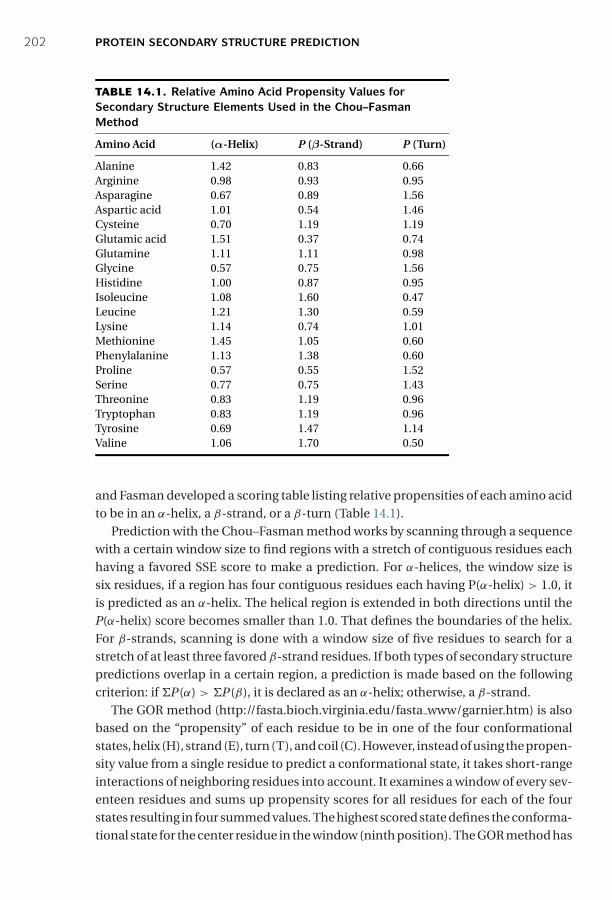
P1: JZP0521840988c14 CB1022/Xiong 0 521 84098 8 January 10, 2006 15:14
202 PROTEIN SECONDARY STRUCTURE PREDICTION
TABLE 14.1. Relative Amino Acid Propensity Values forSecondary Structure Elements Used in the Chou–FasmanMethod
Amino Acid (α-Helix) P (β-Strand) P (Turn)
Alanine 1.42 0.83 0.66Arginine 0.98 0.93 0.95Asparagine 0.67 0.89 1.56Aspartic acid 1.01 0.54 1.46Cysteine 0.70 1.19 1.19Glutamic acid 1.51 0.37 0.74Glutamine 1.11 1.11 0.98Glycine 0.57 0.75 1.56Histidine 1.00 0.87 0.95Isoleucine 1.08 1.60 0.47Leucine 1.21 1.30 0.59Lysine 1.14 0.74 1.01Methionine 1.45 1.05 0.60Phenylalanine 1.13 1.38 0.60Proline 0.57 0.55 1.52Serine 0.77 0.75 1.43Threonine 0.83 1.19 0.96Tryptophan 0.83 1.19 0.96Tyrosine 0.69 1.47 1.14Valine 1.06 1.70 0.50
and Fasman developed a scoring table listing relative propensities of each amino acidto be in an α-helix, a β-strand, or a β-turn (Table 14.1).
Prediction with the Chou–Fasman method works by scanning through a sequencewith a certain window size to find regions with a stretch of contiguous residues eachhaving a favored SSE score to make a prediction. For α-helices, the window size issix residues, if a region has four contiguous residues each having P(α-helix) > 1.0, itis predicted as an α-helix. The helical region is extended in both directions until theP(α-helix) score becomes smaller than 1.0. That defines the boundaries of the helix.For β-strands, scanning is done with a window size of five residues to search for astretch of at least three favored β-strand residues. If both types of secondary structurepredictions overlap in a certain region, a prediction is made based on the followingcriterion: if �P(α) > �P(β), it is declared as an α-helix; otherwise, a β-strand.
The GOR method (http://fasta.bioch.virginia.edu/fasta www/garnier.htm) is alsobased on the “propensity” of each residue to be in one of the four conformationalstates, helix (H), strand (E), turn (T), and coil (C). However, instead of using the propen-sity value from a single residue to predict a conformational state, it takes short-rangeinteractions of neighboring residues into account. It examines a window of every sev-enteen residues and sums up propensity scores for all residues for each of the fourstates resulting in four summed values. The highest scored state defines the conforma-tional state for the center residue in the window (ninth position). The GOR method has
P1: JZP0521840988c14 CB1022/Xiong 0 521 84098 8 January 10, 2006 15:14
SECONDARY STRUCTURE PREDICTION FOR GLOBULAR PROTEINS 203
been shown to be more accurate than Chou–Fasman because it takes the neighboringeffect of residues into consideration.
Both the Chou–Fasman and GOR methods, which are the first-generation methodsdeveloped in the 1970s, suffer from the fact that the prediction rules are somewhatarbitrary. They are based on single sequence statistics without clear relation to knownprotein-folding theories. The predictions solely rely on local sequence informationand fail to take into account long range interactions. A Chou-Fasman–based predictiondoes not even consider the short-range environmental information. These reasons,combined with unreliable statistics derived from a very small structural database,limit the prediction accuracy of these methods to about 50%. This performance isconsidered dismal; any random prediction can have a 40% accuracy given the factthat, in globular proteins, the three-state distribution is 30% α-helix, 20% β-strands,and 50% coil.
Newer algorithms have since been developed to overcome some of these short-comings. The improvements include more refined residue statistics based on alarger number of solved protein structures and the incorporation of more localresidue interactions. Examples of the improved algorithms are GOR II, GOR III,GOR IV, and SOPM. These tools can be found at http://npsa-pbil.ibcp.fr/cgi-bin/npsa automat.pl?page=/NPSA/npsa server.html. These are the second-generationprediction algorithms developed in the 1980s and early 1990s. They have improvedaccuracy over the first generation by about 10%. Although it is already significantlybetter than that by random prediction, the programs are still not reliable enough forroutine application. Prediction errors mainly occur through missed β-strands andshort-lengthed secondary structures for both helices and strands. Prediction of β-strands is still somewhat random. This may be attributed to the fact that long rangeinteractions are not sufficiently taken into consideration in these algorithms.
Homology-Based Methods
The third generation of algorithms were developed in the late 1990s by making useof evolutionary information. This type of method combines the ab initio secondarystructure prediction of individual sequences and alignment information from mul-tiple homologous sequences (>35% identity). The idea behind this approach is thatclose protein homologs should adopt the same secondary and tertiary structure. Wheneach individual sequence is predicted for secondary structure using a method similarto the GOR method, errors and variations may occur. However, evolutionary conser-vation dictates that there should be no major variations for their secondary structureelements. Therefore, by aligning multiple sequences, information of positional con-servation is revealed. Because residues in the same aligned position are assumedto have the same secondary structure, any inconsistencies or errors in prediction ofindividual sequences can be corrected using a majority rule (Fig. 14.1). This homology-based method has helped improve the prediction accuracy by another 10% over thesecond-generation methods.
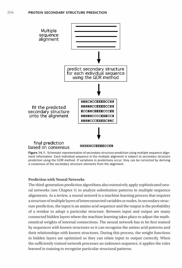
P1: JZP0521840988c14 CB1022/Xiong 0 521 84098 8 January 10, 2006 15:14
204 PROTEIN SECONDARY STRUCTURE PREDICTION
Figure 14.1: Schematic representation of secondary structure prediction using multiple sequence align-ment information. Each individual sequence in the multiple alignment is subject to secondary structureprediction using the GOR method. If variations in predictions occur, they can be corrected by derivinga consensus of the secondary structure elements from the alignment.
Prediction with Neural NetworksThe third-generation prediction algorithms also extensively apply sophisticated neu-ral networks (see Chapter 8) to analyze substitution patterns in multiple sequencealignments. As a review, a neural network is a machine learning process that requiresa structure of multiple layers of interconnected variables or nodes. In secondary struc-ture prediction, the input is an amino acid sequence and the output is the probabilityof a residue to adopt a particular structure. Between input and output are manyconnected hidden layers where the machine learning takes place to adjust the math-ematical weights of internal connections. The neural network has to be first trainedby sequences with known structures so it can recognize the amino acid patterns andtheir relationships with known structures. During this process, the weight functionsin hidden layers are optimized so they can relate input to output correctly. Whenthe sufficiently trained network processes an unknown sequence, it applies the ruleslearned in training to recognize particular structural patterns.

P1: JZP0521840988c14 CB1022/Xiong 0 521 84098 8 January 10, 2006 15:14
SECONDARY STRUCTURE PREDICTION FOR GLOBULAR PROTEINS 205
When multiple sequence alignments and neural networks are combined, the resultis further improved accuracy. In this situation, a neural network is trained not by asingle sequence but by a sequence profile derived from the multiple sequence align-ment. This combined approach has been shown to improve the accuracy to above75%, which is a breakthrough in secondary structure prediction. The improvementmainly comes from enhanced secondary structure signals through consensus draw-ing. The following lists several frequently used third generation prediction algorithmsavailable as web servers.
PHD (Profile network from Heidelberg; http://dodo.bioc.columbia.edu/predictprotein/submit def.html) is a web-based program that combines neural network withmultiple sequence alignment. It first performs a BLASTP of the query sequence againsta nonredundant protein sequence database to find a set of homologous sequences,which are aligned with the MAXHOM program (a weighted dynamic programmingalgorithm performing global alignment). The resulting alignment in the form of aprofile is fed into a neural network that contains three hidden layers. The first hiddenlayer makes raw prediction based on the multiple sequence alignment by sliding awindow of thirteen positions. As in GOR, the prediction is made for the residue in thecenter of the window. The second layer refines the raw prediction by sliding a win-dow of seventeen positions, which takes into account more flanking positions. Thisstep makes adjustments and corrections of unfeasible predictions from the previousstep. The third hidden layer is called the jury network, and contains networks trainedin various ways. It makes final filtering by deleting extremely short helices (one ortwo residues long) and converting them into coils (Fig. 14.2). After the correction, thehighest scored state defines the conformational state of the residue.
PSIPRED (http://bioinf.cs.ucl.ac.uk/psiform.html) is a web-based program thatpredicts protein secondary structures using a combination of evolutionary infor-mation and neural networks. The multiple sequence alignment is derived from aPSI-BLAST database search. A profile is extracted from the multiple sequence align-ment generated from three rounds of automated PSI-BLAST. The profile is then usedas input for a neural network prediction similar to that in PHD, but without the jurylayer. To achieve higher accuracy, a unique filtering algorithm is implemented to filterout unrelated PSI-BLAST hits during profile construction.
SSpro (http://promoter.ics.uci.edu/BRNN-PRED/) is a web-based program thatcombines PSI-BLAST profiles with an advanced neural network, known as bidirec-tional recurrent neural networks (BRNNs). Traditional neural networks are unidirec-tional, feed-forward systems with the information flowing in one direction from inputto output. BRNNs are unique in that the connections of layers are designed to be able togo backward. In this process, known as back propagation, the weights in hidden layersare repeatedly refined. In predicting secondary structure elements, the network usesthe sequence profile as input and finds residue correlations by iteratively recyclingthe network (recursive network). The averaged output from the iterations is given as afinal residue prediction. PROTER (http://distill.ucd.ie/porter/) is a recently developedprogram that uses similar BRNNs and has been shown to slightly outperform SSPRO.

P1: JZP0521840988c14 CB1022/Xiong 0 521 84098 8 January 10, 2006 15:14
206 PROTEIN SECONDARY STRUCTURE PREDICTION
Figure 14.2: Schematic representation of secondary structure prediction in the PHD algorithm usingneural networks. Multiple sequences derived from the BLAST search are used to compile a profile. Theresulting profile is fed into a neural network, which contains three layers – two network layers andone jury layer. The first layer scans thirteen residues per window and makes a raw prediction, which isrefined by the second layer, which scans seventeen residues per window. The third layer makes furtheradjustment to make a final prediction. Adjustment of prediction scores for one amino acid residue isshown.
PROF (Protein forecasting; www.aber.ac.uk/∼phiwww/prof/) is an algorithm thatcombines PSI-BLAST profiles and a multistaged neural network, similar to that inPHD. In addition, it uses a linear discriminant function to discriminate between thethree states.
HMMSTR (Hidden Markov model [HMM] for protein STRuctures; www.bioinfo.rpi.edu/∼bystrc/hmmstr/server.php) uses a branched and cyclic HMM to predictsecondary structures. It first breaks down the query sequence into many very shortsegments (three to nine residues, called I-sites) and builds profiles based on a libraryof known structure motifs. It then assembles these local motifs into a supersecondarystructure. It further uses an HMM with a unique topology linking many smaller HMMsinto a highly branched multicyclic form. This is intended to better capture the recur-rent local features of secondary structure based on multiple sequence alignment.

P1: JZP0521840988c14 CB1022/Xiong 0 521 84098 8 January 10, 2006 15:14
SECONDARY STRUCTURE PREDICTION FOR GLOBULAR PROTEINS 207
Prediction with Multiple MethodsBecause no individual methods can always predict secondary structures correctly, itis desirable to combine predictions from multiple programs with the hope of furtherimproving the accuracy. In fact, a number of web servers have been specifically dedi-cated to making predictions by drawing consensus from results by multiple programs.In many cases, the consensus-based prediction method has been shown to performslightly better than any single method.
Jpred (www.compbio.dundee.ac.uk/∼www-jpred/) combines the analysis resultsfrom six prediction algorithms, including PHD, PREDATOR, DSC, NNSSP, Jnet, andZPred. The query sequence is first used to search databases with PSI-BLAST for threeiterations. Redundant sequence hits are removed. The resulting sequence homologsare used to build a multiple alignment from which a profile is extracted. The profileinformation is submitted to the six prediction programs. If there is sufficient agree-ment among the prediction programs, the majority of the prediction is taken as thestructure. Where there is no majority agreement in the prediction outputs, the PHDprediction is taken.
PredictProtein (www.embl-heidelberg.de/predictprotein/predictprotein.html) isanother multiple prediction server that uses Jpred, PHD, PROF, and PSIPRED, amongothers. The difference is that the server does not run the individual programs butsends the query to other servers which e-mail the results to the user separately. It doesnot generate a consensus. It is up to the user to combine multiple prediction resultsand derive a consensus.
Comparison of Prediction Accuracy
An important issue in protein secondary structure prediction is estimation of theprediction accuracy. The most commonly used measure for cross-validation is knownas a Q3 score, based on the three-state classification, helix (H), strand (E), and coil(C). The score is a percentage of residues of a protein that are correctly predicted.It is normally derived from the average result obtained from the testing with manyproteins with known structures. For secondary structure prediction, there are well-established benchmarks for such prediction evaluation. By using these benchmarks,accuracies for several third-generation prediction algorithms have been compiled(Table 14.2).
As shown in Table 14.2, some of these best prediction methods have reached anaccuracy level around 79% in the three-state prediction. Common errors include theconfusion of helices and strands, incorrect start and end positions of helices andstrands, and missed or wrongly assigned secondary structure elements. If a predictionis consistently 79% accurate, that means on average 21% of the residues could bepredicted incorrectly.
Because different secondary structure prediction programs tend to give variedresults, to maximize the accuracy of prediction, it is recommended to use several mostrobust prediction methods (such as Porter, PROF, and SSPRO) and draw a consensusbased on the majority rule. The aforementioned metaservers provide a convenient
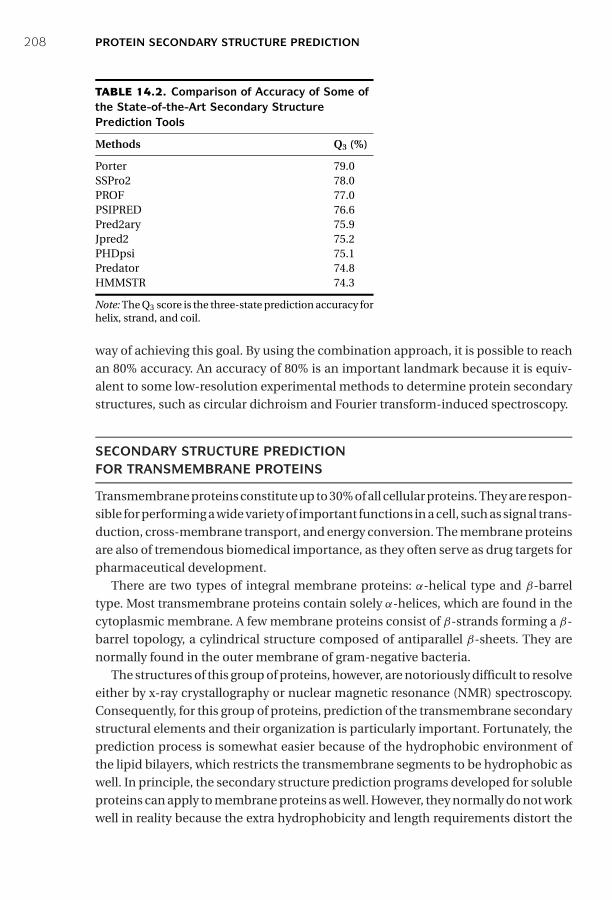
P1: JZP0521840988c14 CB1022/Xiong 0 521 84098 8 January 10, 2006 15:14
208 PROTEIN SECONDARY STRUCTURE PREDICTION
TABLE 14.2. Comparison of Accuracy of Some ofthe State-of-the-Art Secondary StructurePrediction Tools
Methods Q3 (%)
Porter 79.0SSPro2 78.0PROF 77.0PSIPRED 76.6Pred2ary 75.9Jpred2 75.2PHDpsi 75.1Predator 74.8HMMSTR 74.3
Note: The Q3 score is the three-state prediction accuracy forhelix, strand, and coil.
way of achieving this goal. By using the combination approach, it is possible to reachan 80% accuracy. An accuracy of 80% is an important landmark because it is equiv-alent to some low-resolution experimental methods to determine protein secondarystructures, such as circular dichroism and Fourier transform-induced spectroscopy.
SECONDARY STRUCTURE PREDICTIONFOR TRANSMEMBRANE PROTEINS
Transmembrane proteins constitute up to 30% of all cellular proteins. They are respon-sible for performing a wide variety of important functions in a cell, such as signal trans-duction, cross-membrane transport, and energy conversion. The membrane proteinsare also of tremendous biomedical importance, as they often serve as drug targets forpharmaceutical development.
There are two types of integral membrane proteins: α-helical type and β-barreltype. Most transmembrane proteins contain solely α-helices, which are found in thecytoplasmic membrane. A few membrane proteins consist of β-strands forming a β-barrel topology, a cylindrical structure composed of antiparallel β-sheets. They arenormally found in the outer membrane of gram-negative bacteria.
The structures of this group of proteins, however, are notoriously difficult to resolveeither by x-ray crystallography or nuclear magnetic resonance (NMR) spectroscopy.Consequently, for this group of proteins, prediction of the transmembrane secondarystructural elements and their organization is particularly important. Fortunately, theprediction process is somewhat easier because of the hydrophobic environment ofthe lipid bilayers, which restricts the transmembrane segments to be hydrophobic aswell. In principle, the secondary structure prediction programs developed for solubleproteins can apply to membrane proteins as well. However, they normally do not workwell in reality because the extra hydrophobicity and length requirements distort the
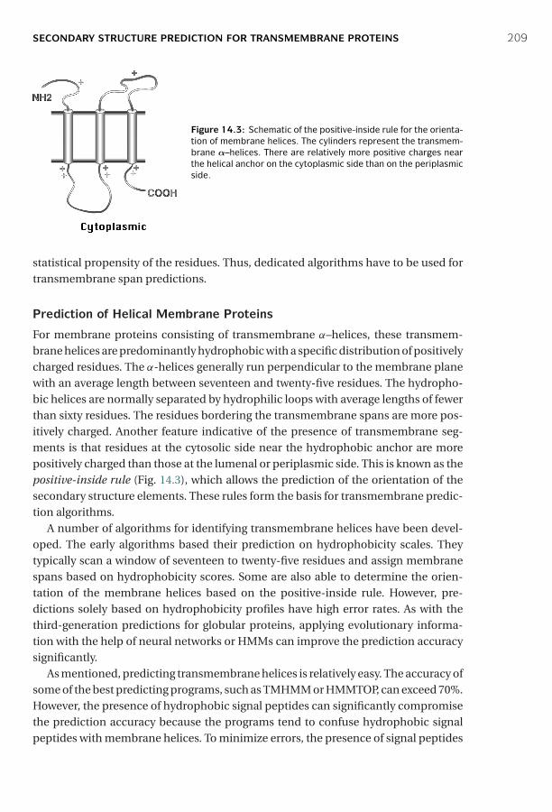
P1: JZP0521840988c14 CB1022/Xiong 0 521 84098 8 January 10, 2006 15:14
SECONDARY STRUCTURE PREDICTION FOR TRANSMEMBRANE PROTEINS 209
Figure 14.3: Schematic of the positive-inside rule for the orienta-tion of membrane helices. The cylinders represent the transmem-brane α–helices. There are relatively more positive charges nearthe helical anchor on the cytoplasmic side than on the periplasmicside.
statistical propensity of the residues. Thus, dedicated algorithms have to be used fortransmembrane span predictions.
Prediction of Helical Membrane Proteins
For membrane proteins consisting of transmembrane α–helices, these transmem-brane helices are predominantly hydrophobic with a specific distribution of positivelycharged residues. The α-helices generally run perpendicular to the membrane planewith an average length between seventeen and twenty-five residues. The hydropho-bic helices are normally separated by hydrophilic loops with average lengths of fewerthan sixty residues. The residues bordering the transmembrane spans are more pos-itively charged. Another feature indicative of the presence of transmembrane seg-ments is that residues at the cytosolic side near the hydrophobic anchor are morepositively charged than those at the lumenal or periplasmic side. This is known as thepositive-inside rule (Fig. 14.3), which allows the prediction of the orientation of thesecondary structure elements. These rules form the basis for transmembrane predic-tion algorithms.
A number of algorithms for identifying transmembrane helices have been devel-oped. The early algorithms based their prediction on hydrophobicity scales. Theytypically scan a window of seventeen to twenty-five residues and assign membranespans based on hydrophobicity scores. Some are also able to determine the orien-tation of the membrane helices based on the positive-inside rule. However, pre-dictions solely based on hydrophobicity profiles have high error rates. As with thethird-generation predictions for globular proteins, applying evolutionary informa-tion with the help of neural networks or HMMs can improve the prediction accuracysignificantly.
As mentioned, predicting transmembrane helices is relatively easy. The accuracy ofsome of the best predicting programs, such as TMHMM or HMMTOP, can exceed 70%.However, the presence of hydrophobic signal peptides can significantly compromisethe prediction accuracy because the programs tend to confuse hydrophobic signalpeptides with membrane helices. To minimize errors, the presence of signal peptides
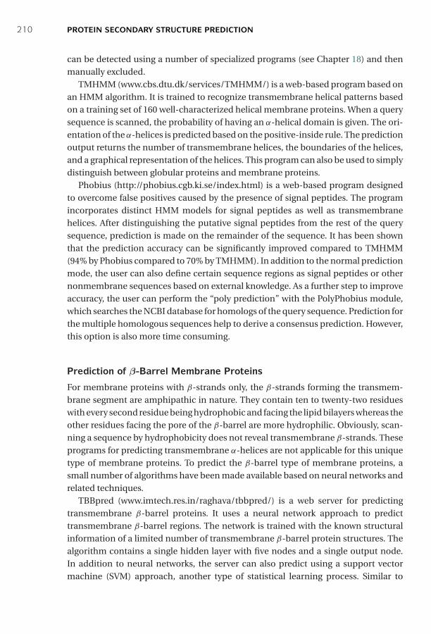
P1: JZP0521840988c14 CB1022/Xiong 0 521 84098 8 January 10, 2006 15:14
210 PROTEIN SECONDARY STRUCTURE PREDICTION
can be detected using a number of specialized programs (see Chapter 18) and thenmanually excluded.
TMHMM (www.cbs.dtu.dk/services/TMHMM/) is a web-based program based onan HMM algorithm. It is trained to recognize transmembrane helical patterns basedon a training set of 160 well-characterized helical membrane proteins. When a querysequence is scanned, the probability of having an α-helical domain is given. The ori-entation of the α-helices is predicted based on the positive-inside rule. The predictionoutput returns the number of transmembrane helices, the boundaries of the helices,and a graphical representation of the helices. This program can also be used to simplydistinguish between globular proteins and membrane proteins.
Phobius (http://phobius.cgb.ki.se/index.html) is a web-based program designedto overcome false positives caused by the presence of signal peptides. The programincorporates distinct HMM models for signal peptides as well as transmembranehelices. After distinguishing the putative signal peptides from the rest of the querysequence, prediction is made on the remainder of the sequence. It has been shownthat the prediction accuracy can be significantly improved compared to TMHMM(94% by Phobius compared to 70% by TMHMM). In addition to the normal predictionmode, the user can also define certain sequence regions as signal peptides or othernonmembrane sequences based on external knowledge. As a further step to improveaccuracy, the user can perform the “poly prediction” with the PolyPhobius module,which searches the NCBI database for homologs of the query sequence. Prediction forthe multiple homologous sequences help to derive a consensus prediction. However,this option is also more time consuming.
Prediction of β-Barrel Membrane Proteins
For membrane proteins with β-strands only, the β-strands forming the transmem-brane segment are amphipathic in nature. They contain ten to twenty-two residueswith every second residue being hydrophobic and facing the lipid bilayers whereas theother residues facing the pore of the β-barrel are more hydrophilic. Obviously, scan-ning a sequence by hydrophobicity does not reveal transmembrane β-strands. Theseprograms for predicting transmembrane α-helices are not applicable for this uniquetype of membrane proteins. To predict the β-barrel type of membrane proteins, asmall number of algorithms have been made available based on neural networks andrelated techniques.
TBBpred (www.imtech.res.in/raghava/tbbpred/) is a web server for predictingtransmembrane β-barrel proteins. It uses a neural network approach to predicttransmembrane β-barrel regions. The network is trained with the known structuralinformation of a limited number of transmembrane β-barrel protein structures. Thealgorithm contains a single hidden layer with five nodes and a single output node.In addition to neural networks, the server can also predict using a support vectormachine (SVM) approach, another type of statistical learning process. Similar to
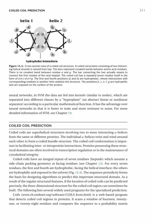
P1: JZP0521840988c14 CB1022/Xiong 0 521 84098 8 January 10, 2006 15:14
COILED COIL PREDICTION 211
Figure 14.4: Cross-section view of a coiled coil structure. A coiled coil protein consisting of two interact-ing helical strands is viewed from top. The bars represent covalent bonds between amino acid residues.There is no covalent bond between residue a and g. The bar connecting the two actually means toconnect the first residue of the next heptad. The coiled coil has a repeated seven residue motif in theform of a-b-c-d-e-f-g. The first and fourth positions (a and d) are hydrophobic, whose interactions withcorresponding residues in another helix stabilize the structure. The positions b, c, e, f, g are hydrophilicand are exposed on the surface of the protein.
neural networks, in SVM the data are fed into kernels (similar to nodes), which areseparated into different classes by a “hyperplane” (an abstract linear or nonlinearseparator) according to a particular mathematical function. It has the advantage overneural networks in that it is faster to train and more resistant to noise. For moredetailed information of SVM, see Chapter 19.
COILED COIL PREDICTION
Coiled coils are superhelical structures involving two to more interacting α-helicesfrom the same or different proteins. The individual α-helices twist and wind aroundeach other to form a coiled bundle structure. The coiled coil conformation is impor-tant in facilitating inter- or intraprotein interactions. Proteins possessing these struc-tural domains are often involved in transcription regulation or in the maintenance ofcytoskeletal integrity.
Coiled coils have an integral repeat of seven residues (heptads) which assume aside-chain packing geometry at facing residues (see Chapter 12). For every sevenresidues, the first and fourth are hydrophobic, facing the helical interface; the othersare hydrophilic and exposed to the solvent (Fig. 14.4). The sequence periodicity formsthe basis for designing algorithms to predict this important structural domain. As aresult of the regular structural features, if the location of coiled coils can be predictedprecisely, the three-dimensional structure for the coiled coil region can sometimes bebuilt. The following lists several widely used programs for the specialized prediction.
Coils (www.ch.embnet.org/software/COILS form.html) is a web-based programthat detects coiled coil regions in proteins. It scans a window of fourteen, twenty-one, or twenty-eight residues and compares the sequence to a probability matrix
P1: JZP0521840988c14 CB1022/Xiong 0 521 84098 8 January 10, 2006 15:14
212 PROTEIN SECONDARY STRUCTURE PREDICTION
compiled from known parallel two-stranded coiled coils. By comparing the similarityscores, the program calculates the probability of the sequence to adopt a coiled coilconformation. The program is accurate for solvent-exposed, left-handed coiled coils,but less sensitive for other types of coiled coil structures, such as buried or right-handed coiled coils.
Multicoil (http://jura.wi.mit.edu/cgi-bin/multicoil/multicoil.pl) is a web-basedprogram for predicting coiled coils. The scoring matrix is constructed based on adatabase of known two-stranded and three-stranded coiled coils. The program ismore conservative than Coils. It has been recently used in several genome-widestudies to screen for protein–protein interactions mediated by coiled coil domains.
Leucine zipper domains are a special type of coiled coils found in transcription reg-ulatory proteins. They contain two antiparallelα-helices held together by hydrophobicinteractions of leucine residues. The heptad repeat pattern is L-X(6)-L-X(6)-L–X(6)-L.This repeat pattern alone can sometimes allow the domain detection, albeit with highrates of false positives. The reason for the high false-positive rates is that the conditionof the sequence region being a coiled coil conformation is not satisfied. To addressthis problem, algorithms have been developed that take into account both leucinerepeats and coiled coil conformation to give accurate prediction.
2ZIP (http://2zip.molgen.mpg.de/) is a web-based server that predicts leucine zip-pers. It combines searching of the characteristic leucine repeats with coiled coil pre-diction using an algorithm similar to Coils to yield accurate results.
SUMMARY
Protein secondary structure prediction has a long history and is defined by threegenerations of development. The first generation algorithms were ab initio based,examining residue propensities that fall in the three states: helices, strands, and coils.The propensities were derived from a very small structural database. The growingstructural database and use of residue local environment information allowed thedevelopment of the second-generation algorithms. A major breakthrough came fromthe third-generation algorithms that make use of multiple sequence alignment infor-mation, which implicitly takes the long-range intraprotein interactions into consid-eration. In combination with neural networks and other sophisticated algorithms,prediction efficiency has been improved significantly. To achieve high accuracy in pre-diction, combining results from several top-performing third-generation algorithmsis recommended. Predicting secondary structures for membrane proteins is morecommon than for globular proteins as crystal or NMR structures are extremely diffi-cult to obtain for the former. The prediction of transmembrane segments (mainlyα-helices) involves the use of hydrophobicity, neural networks, and evolutionaryinformation. Coiled coils are a distinct type of supersecondary structure with reg-ular periodicity of hydrophobic residues that can be predicted using specializedalgorithms.
P1: JZP0521840988c14 CB1022/Xiong 0 521 84098 8 January 10, 2006 15:14
FURTHER READING 213
FURTHER READING
Edwards, Y. J., and Cottage, A. 2003. Bioinformatics methods to predict protein structure andfunction. A practical approach. Mol. Biotechnol. 23:139-66.
Heringa J. 2002. Computational methods for protein secondary structure prediction using mul-tiple sequence alignments. Curr. Protein Pept. Sci. 1:273-301.
Lehnert, U., Xia, Y., Royce, T. E., Goh, C. S., Liu, Y., Senes, A., Yu. H., Zhang, Z. L., Engelman, D. M,and Gerstein M. 2004. Computational analysis of membrane proteins: Genomic occurrence,structure prediction and helix interactions. Q. Rev. Biophys. 37:121-46.
Moller, S., Croning, M. D. R., and Apweiler, R. 2001. Evaluation of methods for the prediction ofmembrane spanning regions. Bioinformatics 17:646-53.
Przybylski, D., and Rost, B. 2002. Alignments grow, secondary structure prediction improves.Proteins 46:197–205.
Rost B. 2001. Review: Protein secondary structure prediction continues to rise. J. Struct. Biol.134:204–18.
———. 2003. Prediction in 1D: Secondary structure, membrane helices, and accessibility. InStructural Bioinformatics, edited by P. E. Bourne and H. Weissig, 559–87. Hoboken, NJ:Wiley–Liss.
P1: KsF0521840988c15 CB1022/Xiong 0 521 84098 8 January 10, 2006 13:58
CHAPTER FIFTEEN
Protein Tertiary Structure Prediction
One of the most important scientific achievements of the twentieth century was thediscovery of the DNA double helical structure by Watson and Crick in 1953. Strictlyspeaking, the work was the result of a three-dimensional modeling conducted partlybased on data obtained from x-ray diffraction of DNA and partly based on chemicalbonding information established in stereochemistry. It was clear at the time thatthe x-ray data obtained by their colleague Rosalind Franklin were not sufficient toresolve the DNA structure. Watson and Crick conducted one of the first-known abinitio modeling of a biological macromolecule, which has subsequently been provento be essentially correct. Their work provided great insight into the mechanism ofgenetic inheritance and paved the way for a revolution in modern biology. The exampledemonstrates that structural prediction is a powerful tool to understand the functionsof biological macromolecules at the atomic level.
We now know that the DNA structure, a double helix, is rather invariable regardlessof sequence variations. Although there is little need today to determine or modelDNA structures of varying sequences, there is still a real need to model proteinstructures individually. This is because protein structures vary depending on thesequences. Another reason is the much slower rate of structure determination byx-ray crystallography or NMR spectroscopy compared to gene sequence generationfrom genomic studies. Consequently, the gap between protein sequence informationand protein structural information is increasing rapidly. Protein structure predictionaims to reduce this sequence–structure gap.
In contrast to sequencing techniques, experimental methods to determine proteinstructures are time consuming and limited in their approach. Currently, it takes 1 to3 years to solve a protein structure. Certain proteins, especially membrane proteins,are extremely difficult to solve by x-ray or NMR techniques. There are many importantproteins for which the sequence information is available, but their three-dimensionalstructures remain unknown. The full understanding of the biological roles of theseproteins requires knowledge of their structures. Hence, the lack of such informationhinders many aspects of the analysis, ranging from protein function and ligand bind-ing to mechanisms of enzyme catalysis. Therefore, it is often necessary to obtainapproximate protein structures through computer modeling.
Having a computer-generated three-dimensional model of a protein of interesthas many ramifications, assuming it is reasonably correct. It may be of use for therational design of biochemical experiments, such as site-directed mutagenesis, pro-tein stability, or functional analysis. In addition to serving as a theoretical guide to
214
P1: KsF0521840988c15 CB1022/Xiong 0 521 84098 8 January 10, 2006 13:58
HOMOLOGY MODELING 215
design experiments for protein characterization, the model can help to rationalizethe experimental results obtained with the protein of interest. In short, the modelingstudy helps to advance our understanding of protein functions.
METHODS
There are three computational approaches to protein three-dimensional structuralmodeling and prediction. They are homology modeling, threading, and ab initio pre-diction. The first two are knowledge-based methods; they predict protein structuresbased on knowledge of existing protein structural information in databases. Homol-ogy modeling builds an atomic model based on an experimentally determined struc-ture that is closely related at the sequence level. Threading identifies proteins thatare structurally similar, with or without detectable sequence similarities. The ab ini-tio approach is simulation based and predicts structures based on physicochemicalprinciples governing protein folding without the use of structural templates.
HOMOLOGY MODELING
As the name suggests, homology modeling predicts protein structures based onsequence homology with known structures. It is also known as comparative mod-eling. The principle behind it is that if two proteins share a high enough sequencesimilarity, they are likely to have very similar three-dimensional structures. If one ofthe protein sequences has a known structure, then the structure can be copied to theunknown protein with a high degree of confidence. Homology modeling produces anall-atom model based on alignment with template proteins.
The overall homology modeling procedure consists of six steps. The first step istemplate selection, which involves identification of homologous sequences in theprotein structure database to be used as templates for modeling. The second step isalignment of the target and template sequences. The third step is to build a frame-work structure for the target protein consisting of main chain atoms. The fourth stepof model building includes the addition and optimization of side chain atoms andloops. The fifth step is to refine and optimize the entire model according to energycriteria. The final step involves evaluating of the overall quality of the model obtained(Fig. 15.1). If necessary, alignment and model building are repeated until a satisfactoryresult is obtained.
Template Selection
The first step in protein structural modeling is to select appropriate structural tem-plates. This forms the foundation for rest of the modeling process. The templateselection involves searching the Protein Data Bank (PDB) for homologous proteinswith determined structures. The search can be performed using a heuristic pairwisealignment search program such as BLAST or FASTA. However, the use of dynamicprogramming based search programs such as SSEARCH or ScanPS (see Chapter 4)

P1: KsF0521840988c15 CB1022/Xiong 0 521 84098 8 January 10, 2006 13:58
216 PROTEIN TERTIARY STRUCTURE PREDICTION
Figure 15.1: Flowchart showing steps involved in homology modeling.
can result in more sensitive search results. The relatively small size of the structuraldatabase means that the search time using the exhaustive method is still within rea-sonable limits, while giving a more sensitive result to ensure the best possible simi-larity hits.
As a rule of thumb, a database protein should have at least 30% sequence identitywith the query sequence to be selected as template. Occasionally, a 20% identity levelcan be used as threshold as long as the identity of the sequence pair falls withinthe “safe zone” (see Chapter 3). Often, multiple database structures with significantsimilarity can be found as a result of the search. In that case, it is recommendedthat the structure(s) with the highest percentage identity, highest resolution, and themost appropriate cofactors is selected as a template. On the other hand, there may be asituation in which no highly similar sequences can be found in the structure database.In that instance, template selection can become difficult. Either a more sensitiveprofile-based PSI-BLAST method or a fold recognition method such threading can beused to identify distant homologs. Most likely, in such a scenario, only local similaritiescan be identified with distant homologs. Modeling can therefore only be done withthe aligned domains of the target protein.
Sequence Alignment
Once the structure with the highest sequence similarity is identified as a template, thefull-length sequences of the template and target proteins need to be realigned usingrefined alignment algorithms to obtain optimal alignment. This realignment is themost critical step in homology modeling, which directly affects the quality of the finalmodel. This is because incorrect alignment at this stage leads to incorrect designationof homologous residues and therefore to incorrect structural models. Errors made inthe alignment step cannot be corrected in the following modeling steps. Therefore,the best possible multiple alignment algorithms, such as Praline and T-Coffee (seeChapter 5), should be used for this purpose. Even alignment using the best alignment
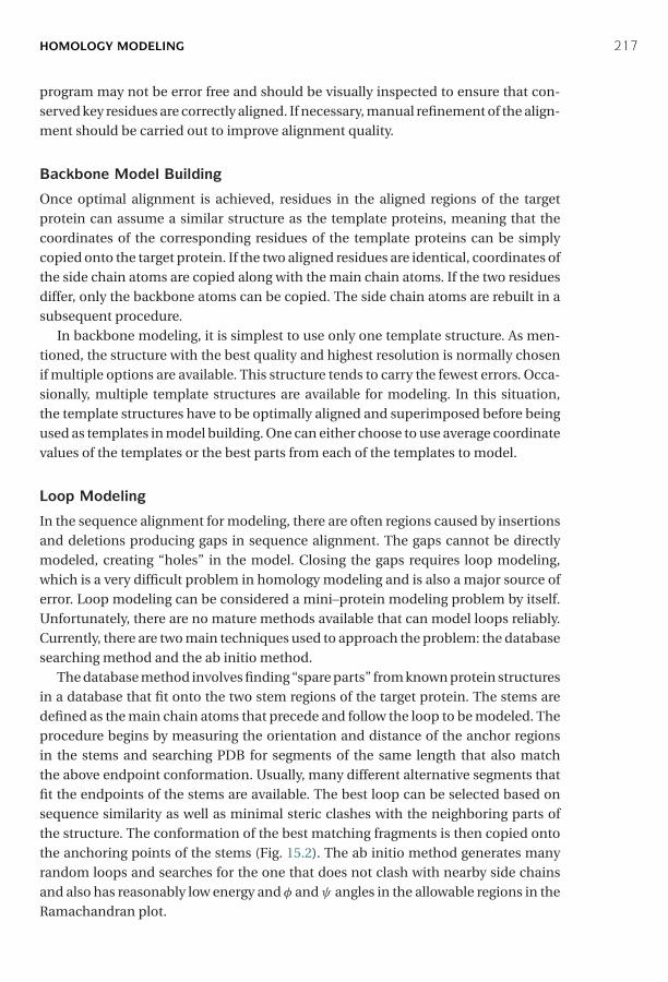
P1: KsF0521840988c15 CB1022/Xiong 0 521 84098 8 January 10, 2006 13:58
HOMOLOGY MODELING 217
program may not be error free and should be visually inspected to ensure that con-served key residues are correctly aligned. If necessary, manual refinement of the align-ment should be carried out to improve alignment quality.
Backbone Model Building
Once optimal alignment is achieved, residues in the aligned regions of the targetprotein can assume a similar structure as the template proteins, meaning that thecoordinates of the corresponding residues of the template proteins can be simplycopied onto the target protein. If the two aligned residues are identical, coordinates ofthe side chain atoms are copied along with the main chain atoms. If the two residuesdiffer, only the backbone atoms can be copied. The side chain atoms are rebuilt in asubsequent procedure.
In backbone modeling, it is simplest to use only one template structure. As men-tioned, the structure with the best quality and highest resolution is normally chosenif multiple options are available. This structure tends to carry the fewest errors. Occa-sionally, multiple template structures are available for modeling. In this situation,the template structures have to be optimally aligned and superimposed before beingused as templates in model building. One can either choose to use average coordinatevalues of the templates or the best parts from each of the templates to model.
Loop Modeling
In the sequence alignment for modeling, there are often regions caused by insertionsand deletions producing gaps in sequence alignment. The gaps cannot be directlymodeled, creating “holes” in the model. Closing the gaps requires loop modeling,which is a very difficult problem in homology modeling and is also a major source oferror. Loop modeling can be considered a mini–protein modeling problem by itself.Unfortunately, there are no mature methods available that can model loops reliably.Currently, there are two main techniques used to approach the problem: the databasesearching method and the ab initio method.
The database method involves finding “spare parts” from known protein structuresin a database that fit onto the two stem regions of the target protein. The stems aredefined as the main chain atoms that precede and follow the loop to be modeled. Theprocedure begins by measuring the orientation and distance of the anchor regionsin the stems and searching PDB for segments of the same length that also matchthe above endpoint conformation. Usually, many different alternative segments thatfit the endpoints of the stems are available. The best loop can be selected based onsequence similarity as well as minimal steric clashes with the neighboring parts ofthe structure. The conformation of the best matching fragments is then copied ontothe anchoring points of the stems (Fig. 15.2). The ab initio method generates manyrandom loops and searches for the one that does not clash with nearby side chainsand also has reasonably low energy and φ and ψ angles in the allowable regions in theRamachandran plot.
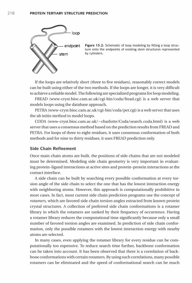
P1: KsF0521840988c15 CB1022/Xiong 0 521 84098 8 January 10, 2006 13:58
218 PROTEIN TERTIARY STRUCTURE PREDICTION
Figure 15.2: Schematic of loop modeling by fitting a loop struc-ture onto the endpoints of existing stem structures representedby cylinders.
If the loops are relatively short (three to five residues), reasonably correct modelscan be built using either of the two methods. If the loops are longer, it is very difficultto achieve a reliable model. The following are specialized programs for loop modeling.
FREAD (www-cryst.bioc.cam.ac.uk/cgi-bin/coda/fread.cgi) is a web server thatmodels loops using the database approach.
PETRA (www-cryst.bioc.cam.ac.uk/cgi-bin/coda/pet.cgi) is a web server that usesthe ab initio method to model loops.
CODA (www-cryst.bioc.cam.ac.uk/∼charlotte/Coda/search coda.html) is a webserver that uses a consensus method based on the prediction results from FREAD andPETRA. For loops of three to eight residues, it uses consensus conformation of bothmethods and for nine to thirty residues, it uses FREAD prediction only.
Side Chain Refinement
Once main chain atoms are built, the positions of side chains that are not modeledmust be determined. Modeling side chain geometry is very important in evaluat-ing protein–ligand interactions at active sites and protein–protein interactions at thecontact interface.
A side chain can be built by searching every possible conformation at every tor-sion angle of the side chain to select the one that has the lowest interaction energywith neighboring atoms. However, this approach is computationally prohibitive inmost cases. In fact, most current side chain prediction programs use the concept ofrotamers, which are favored side chain torsion angles extracted from known proteincrystal structures. A collection of preferred side chain conformations is a rotamerlibrary in which the rotamers are ranked by their frequency of occurrence. Havinga rotamer library reduces the computational time significantly because only a smallnumber of favored torsion angles are examined. In prediction of side chain confor-mation, only the possible rotamers with the lowest interaction energy with nearbyatoms are selected.
In many cases, even applying the rotamer library for every residue can be com-putationally too expensive. To reduce search time further, backbone conformationcan be taken into account. It has been observed that there is a correlation of back-bone conformations with certain rotamers. By using such correlations, many possiblerotamers can be eliminated and the speed of conformational search can be much
P1: KsF0521840988c15 CB1022/Xiong 0 521 84098 8 January 10, 2006 13:58
HOMOLOGY MODELING 219
improved. After adding the most frequently occurring rotamers, the conformationshave to be further optimized to minimize steric overlaps with the rest of the modelstructure.
Most modeling packages incorporate the side chain refinement function. Aspecialized side chain modeling program that has reasonably good performance isSCWRL (sidechain placement with a rotamer library; www.fccc.edu/research/labs/dunbrack/scwrl/), a UNIX program that works by placing side chains on a back-bone template according to preferences in the backbone-dependent rotamer library.It removes rotamers that have steric clashes with main chain atoms. The final, selectedset of rotamers has minimal clashes with main chain atoms and other side chains.
Model Refinement Using Energy Function
In these loop modeling and side chain modeling steps, potential energy calculationsare applied to improve the model. However, this does not guarantee that the entire rawhomology model is free of structural irregularities such as unfavorable bond angles,bond lengths, or close atomic contacts. These kinds of structural irregularities can becorrected by applying the energy minimization procedure on the entire model, whichmoves the atoms in such a way that the overall conformation has the lowest energypotential. The goal of energy minimization is to relieve steric collisions and strainswithout significantly altering the overall structure.
However, energy minimization has to be used with caution because excessiveenergy minimization often moves residues away from their correct positions. There-fore, only limited energy minimization is recommended (a few hundred iterations)to remove major errors, such as short bond distances and close atomic clashes. Keyconserved residues and those involved in cofactor binding have to be restrained ifnecessary during the process.
Another often used structure refinement procedure is molecular dynamic simula-tion. This practice is derived from the concern that energy minimization only movesatoms toward a local minimum without searching for all possible conformations, oftenresulting in a suboptimal structure. To search for a global minimum requires movingatoms uphill as well as downhill in a rough energy landscape. This requires thermo-dynamic calculations of the atoms. In this process, a protein molecule is “heated” or“cooled” to simulate the uphill and downhill molecular motions. Thus, it helps over-come energy hurdles that are inaccessible to energy minimization. It is hoped thatthis simulation follows the protein folding process and has a better chance at findingthe true structure. A more realistic simulation can include water molecules surround-ing the structure. This makes the process an even more computationally expensiveprocedure than energy minimization, however. Furthermore, it shares a similar weak-ness of energy minimization: a molecular structure can be “loosened up” such thatit becomes less realistic. Much caution is therefore needed in using these moleculardynamic tools.
GROMOS (www.igc.ethz.ch/gromos/) is a UNIX program for molecular dynamicsimulation. It is capable of performing energy minimization and thermodynamic

P1: KsF0521840988c15 CB1022/Xiong 0 521 84098 8 January 10, 2006 13:58
220 PROTEIN TERTIARY STRUCTURE PREDICTION
simulation of proteins, nucleic acids, and other biological macromolecules. The sim-ulation can be done in vacuum or in solvents. A lightweight version of GROMOS hasbeen incorporated in SwissPDB Viewer.
Model Evaluation
The final homology model has to be evaluated to make sure that the structural featuresof the model are consistent with the physicochemical rules. This involves checkinganomalies in φ–ψ angles, bond lengths, close contacts, and so on. Another way ofchecking the quality of a protein model is to implicitly take these stereochemicalproperties into account. This is a method that detects errors by compiling statisticalprofiles of spatial features and interaction energy from experimentally determinedstructures. By comparing the statistical parameters with the constructed model, themethod reveals which regions of a sequence appear to be folded normally and whichregions do not. If structural irregularities are found, the region is considered to haveerrors and has to be further refined.
Procheck (www.biochem.ucl.ac.uk/∼roman/procheck/procheck.html) is a UNIXprogram that is able to check general physicochemical parameters such as φ–ψ
angles, chirality, bond lengths, bond angles, and so on. The parameters of the modelare used to compare with those compiled from well-defined, high-resolution struc-tures. If the program detects unusual features, it highlights the regions that should bechecked or refined further.
WHAT IF (www.cmbi.kun.nl:1100/WIWWWI/) is a comprehensive protein analysisserver that validates a protein model for chemical correctness. It has many functions,including checking of planarity, collisions with symmetry axes (close contacts), prolinepuckering, anomalous bond angles, and bond lengths. It also allows the generationof Ramachandran plots as an assessment of the quality of the model.
ANOLEA (Atomic Non-Local Environment Assessment; http://protein.bio.puc.cl/cardex/servers/anolea/index.html) is a web server that uses the statistical evaluationapproach. It performs energy calculations for atomic interactions in a protein chainand compares these interaction energy values with those compiled from a databaseof protein x-ray structures. If the energy terms of certain regions deviate significantlyfrom those of the standard crystal structures, it defines them as unfavorable regions.An example of the output from the verification of a homology model is shown inFigure 15.3A. The threshold for unfavorable residues is normally set at 5.0. Residueswith scores above 5.0 are considered regions with errors.
Verify3D (www.doe-mbi.ucla.edu/Services/Verify 3D/) is another server using thestatistical approach. It uses a precomputed database containing eighteen environ-mental profiles based on secondary structures and solvent exposure, compiled fromhigh-resolution protein structures. To assess the quality of a protein model, the sec-ondary structure and solvent exposure propensity of each residue are calculated. If theparameters of a residue fall within one of the profiles, it receives a high score, other-wise a low score. The result is a two-dimensional graph illustrating the folding qualityof each residue of the protein structure. A verification output of the above homology
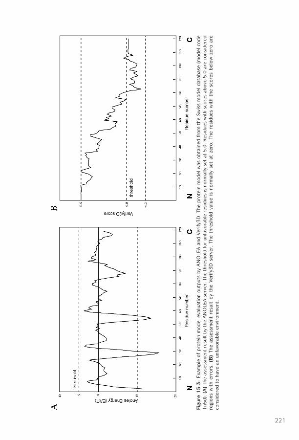
P1: KsF0521840988c15 CB1022/Xiong 0 521 84098 8 January 10, 2006 13:58
Figu
re1
5.3
:Ex
ample
ofpro
tein
mod
elev
alua
tion
outp
uts
by
AN
OLE
Aan
dVe
rify
3D
.Th
epro
tein
mod
elw
asob
tain
edfr
omth
eSw
iss
mod
eldat
abas
e(m
odel
code
1n5
d).
(A)
The
asse
ssm
ent
resu
ltby
the
AN
OLE
Ase
rver
.The
thre
shol
dfo
run
favo
rable
resi
due
sis
norm
ally
set
at5.0
.Res
idue
sw
ith
scor
esab
ove
5.0
are
cons
ider
edre
gion
sw
ith
erro
rs.
(B)
The
asse
ssm
ent
resu
ltby
the
Veri
fy3D
serv
er.
The
thre
shol
dva
lue
isno
rmal
lyse
tat
zero
.Th
ere
sidue
sw
ith
the
scor
esbel
owze
roar
eco
nsid
ered
toha
vean
unfa
vora
ble
envi
ronm
ent.
221
P1: KsF0521840988c15 CB1022/Xiong 0 521 84098 8 January 10, 2006 13:58
222 PROTEIN TERTIARY STRUCTURE PREDICTION
model is shown in Figure 15.3B. The threshold value is normally set at zero. Residueswith scores below zero are considered to have an unfavorable environment.
The assessment results can be different using different verification programs. Asshown in Figure 15.2, ANOLEA appears to be less stringent than Verify3D. Although thefull-length protein chain of this model is declared favorable by ANOLEA, residues inthe C-terminus of the protein are considered to be of low quality by Verify3D. Becauseno single method is clearly superior to any other, a good strategy is to use multipleverification methods and identify the consensus between them. It is also importantto keep in mind that the evaluation tests performed by these programs only checkthe stereochemical correctness, regardless of the accuracy of the model, which mayor may not have any biological meaning.
Comprehensive Modeling Programs
A number of comprehensive modeling programs are able to perform the completeprocedure of homology modeling in an automated fashion. The automation requiresassembling a pipeline that includes target selection, alignment, model generation,and model evaluation. Some freely available protein modeling programs and serversare listed.
Modeller (http://bioserv.cbs.cnrs.fr/HTML BIO/frame mod.html) is a web serverfor homology modeling. The user provides a predetermined sequence alignment ofa template(s) and a target to allow the program to calculate a model containing allof the heavy atoms (nonhydrogen atoms). The program models the backbone usinga homology-derived restraint method, which relies on multiple sequence alignmentbetween target and template proteins to distinguish highly conserved residues fromless conserved ones. Conserved residues are given high restraints in copying fromthe template structures. Less conserved residues, including loop residues, are givenless or no restraints, so that their conformations can be built in a more or less abinitio fashion. The entire model is optimized by energy minimization and moleculardynamics procedures.
Swiss-Model (www.expasy.ch/swissmod/SWISS-MODEL.html) is an automatedmodeling server that allows a user to submit a sequence and to get back a structureautomatically. The server constructs a model by automatic alignment (First Approachmode) or manual alignment (Optimize mode). In the First Approach mode, the userprovides sequence input for modeling. The server performs alignment of the querywith sequences in PDB using BLAST. After selection of suitable templates, a raw modelis built. Refinement of the structure is done using GROMOS. Alternatively, the user canspecify or upload structures as templates. The final model is sent to the user by e-mail.In the Optimize mode, the user constructs a sequence alignment in SwissPdbViewerand submits it to the server for model construction.
3D-JIGSAW (www.bmm.icnet.uk/servers/3djigsaw/) is a modeling server thatworks in either the automatic mode or the interactive mode. Its loop modeling relieson the database method. The interactive mode allows the user to edit alignmentsand select templates, loops, and side chains during modeling, whereas the automatic
P1: KsF0521840988c15 CB1022/Xiong 0 521 84098 8 January 10, 2006 13:58
THREADING AND FOLD RECOGNITION 223
mode allows no human intervention and models a submitted protein sequence if ithas an identity >40% with known protein structures.
Homology Model Databases
The availability of automated modeling algorithms has allowed several researchgroups to use the fully automated procedure to carry out large-scale modelingprojects. Protein models for entire sequence databases or entire translated genomeshave been generated. Databases for modeled protein structures that include nearlyone third of all known proteins have been established. They provide some useful infor-mation for understanding evolution of protein structures. The large databases can alsoaid in target selection for drug development. However, it has also been shown thatthe automated procedure is unable to model moderately distant protein homologs.Automated modeling tends to be less accurate than modeling that requires humanintervention because of inappropriate template selection, suboptimal alignment, anddifficulties in modeling loops and side chains.
ModBase (http://alto.compbio.ucsf.edu/modbase-cgi/index.cgi) is a database ofprotein models generated by the Modeller program. For most sequences that havebeen modeled, only partial sequences or domains that share strong similarities withtemplates are actually modeled.
3Dcrunch (www.expasy.ch/swissmod/SWISS-MODEL.html) is another databasearchiving results of large-scale homology modeling projects. Models of partialsequences from the Swiss-Prot database are derived using the Swiss-Model program.
THREADING AND FOLD RECOGNITION
As discussed in Chapters 12 and 13, there are only small number of protein foldsavailable (<1,000), compared to millions of protein sequences. This means that pro-tein structures tend to be more conserved than protein sequences. Consequently,many proteins can share a similar fold even in the absence of sequence similarities.This allowed the development of computational methods to predict protein struc-tures beyond sequence similarities. To determine whether a protein sequence adoptsa known three-dimensional structure fold relies on threading and fold recognitionmethods.
By definition, threading or structural fold recognition predicts the structural fold ofan unknown protein sequence by fitting the sequence into a structural database andselecting the best-fitting fold. The comparison emphasizes matching of secondarystructures, which are most evolutionarily conserved. Therefore, this approach canidentify structurally similar proteins even without detectable sequence similarity.
The algorithms can be classified into two categories, pairwise energy based andprofile based. The pairwise energy–based method was originally referred to as thread-ing and the profile-based method was originally defined as fold recognition. How-ever, the two terms are now often used interchangeably without distinction in theliterature.

P1: KsF0521840988c15 CB1022/Xiong 0 521 84098 8 January 10, 2006 13:58
224 PROTEIN TERTIARY STRUCTURE PREDICTION
Figure 15.4: Outline of the threading method using the pairwise energy approach to predict proteinstructural folds from sequence. By fitting a structural fold library and assessing the energy terms of theresulting raw models, the best-fit structural fold can be selected.
Pairwise Energy Method
In the pairwise energy based method, a protein sequence is searched for in a structuralfold database to find the best matching structural fold using energy-based criteria.The detailed procedure involves aligning the query sequence with each structuralfold in a fold library. The alignment is performed essentially at the sequence profilelevel using dynamic programming or heuristic approaches. Local alignment is oftenadjusted to get lower energy and thus better fitting. The adjustment can be achievedusing algorithms such as double-dynamic programming (see Chapter 14). The nextstep is to build a crude model for the target sequence by replacing aligned residues inthe template structure with the corresponding residues in the query. The third stepis to calculate the energy terms of the raw model, which include pairwise residueinteraction energy, solvation energy, and hydrophobic energy. Finally, the models areranked based on the energy terms to find the lowest energy fold that corresponds tothe structurally most compatible fold (Fig. 15.4).
Profile Method
In the profile-based method, a profile is constructed for a group of related proteinstructures. The structural profile is generated by superimposition of the structures toexpose corresponding residues. Statistical information from these aligned residues isthen used to construct a profile. The profile contains scores that describe the propen-sity of each of the twenty amino acid residues to be at each profile position. The profile

P1: KsF0521840988c15 CB1022/Xiong 0 521 84098 8 January 10, 2006 13:58
THREADING AND FOLD RECOGNITION 225
scores contain information for secondary structural types, the degree of solvent expo-sure, polarity, and hydrophobicity of the amino acids. To predict the structural fold ofan unknown query sequence, the query sequence is first predicted for its secondarystructure, solvent accessibility, and polarity. The predicted information is then usedfor comparison with propensity profiles of known structural folds to find the fold thatbest represents the predicted profile.
Because threading and fold recognition detect structural homologs without com-pletely relying on sequence similarities, they have been shown to be far more sensitivethan PSI-BLAST in finding distant evolutionary relationships. In many cases, they canidentify more than twice as many distant homologs than PSI-BLAST. However, thishigh sensitivity can also be their weakness because high sensitivity is often associatedwith low specificity. The predictions resulting from threading and fold recognitionoften come with very high rates of false positives. Therefore, much caution is requiredin accepting the prediction results.
Threading and fold recognition assess the compatibility of an amino acid sequencewith a known structure in a fold library. If the protein fold to be predicted does not existin the fold library, the method will fail. Another disadvantage compared to homologymodeling lies in the fact that threading and fold recognition do not generate fullyrefined atomic models for the query sequences. This is because accurate alignmentbetween distant homologs is difficult to achieve. Instead, threading and fold recog-nition procedures only provide a rough approximation of the overall topology of thenative structure.
A number of threading and fold recognition programs are available using either orboth prediction strategies. At present, no single algorithm is always able to providereliable fold predictions. Some algorithms work well with some types of structures,but fail with others. It is a good practice to compare results from multiple programsfor consistency and judge the correctness by using external knowledge.
3D-PSSM (www.bmm.icnet.uk/∼3dpssm/) is a web-based program that employsthe structural profile method to identify protein folds. The profiles for each proteinsuperfamily are constructed by combining multiple smaller profiles. First, proteinstructures in a superfamily based on the SCOP classification are superimposed andare used to construct a structural profile by incorporating secondary structures andsolvent accessibility information for corresponding residues. In addition, each mem-ber in a protein structural superfamily has its own sequence-based PSI-BLAST profilecomputed. These sequence profiles are used in combination with the structure pro-file to form a large superfamily profile in which each position contains both sequenceand structural information. For the query sequence, PSI-BLAST is performed to gen-erate a sequence-based profile. PSI-PRED is used to predict its secondary struc-ture. Both the sequence profile and predicted secondary structure are comparedwith the precomputed protein superfamily profiles, using a dynamic programmingapproach. The matching scores are calculated in terms of secondary structure, solva-tion energy, and sequence profiles and ranked to find the highest scored structure fold(Fig. 15.5).
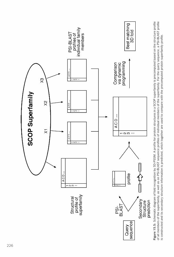
P1: KsF0521840988c15 CB1022/Xiong 0 521 84098 8 January 10, 2006 13:58
Figu
re1
5.5
:Sch
emat
icdia
gram
offo
ldre
cogn
itio
nby
3D
-PSSM
.Apro
file
for
pro
tein
stru
ctur
esin
aSC
OP
super
fam
ilyis
pre
com
put
edbas
edon
the
stru
ctur
epro
file
ofal
lmem
ber
sof
the
super
fam
ily,
asw
ella
son
PSI-
BLA
ST
seque
nce
pro
files
ofin
div
idua
lmem
ber
sof
the
super
fam
ily.
For
the
que
ryse
que
nce,
aP
SI-
BLA
ST
pro
file
isco
nstr
ucte
dan
dits
seco
ndar
yst
ruct
ure
info
rmat
ion
ispre
dic
ted,
whi
chto
geth
erar
eus
edto
com
par
ew
ith
the
pre
com
put
edpro
tein
super
fam
ilypro
file.
226
P1: KsF0521840988c15 CB1022/Xiong 0 521 84098 8 January 10, 2006 13:58
AB INITIO PROTEIN STRUCTURAL PREDICTION 227
GenThreader (http://bioinf.cs.ucl.ac.uk/psipred/index.html) is a web-based pro-gram that uses a hybrid of the profile and pairwise energy methods. The initial stepis similar to 3D-PSSM; the query protein sequence is subject to three rounds ofPSI-BLAST. The resulting multiple sequence hits are used to generate a profile. Itssecondary structure is predicted using PSIPRED. Both are used as input for threadingcomputation based on a pairwise energy potential method. The threading results areevaluated using neural networks that combine energy potentials, sequence alignmentscores, and length information to create a single score representing the relationshipbetween the query and template proteins.
Fugue (www-cryst.bioc.cam.ac.uk/∼fugue/prfsearch.html) is a profile-based foldrecognition server. It has precomputed structural profiles compiled from multiplealignments of homologous structures, which take into account local structural envi-ronment such as secondary structure, solvent accessibility, and hydrogen bondingstatus. The query sequence (or a multiple sequence alignment if the user prefers) isused to scan the database of structural profiles. The comparison between the queryand the structural profiles is done using global alignment or local alignment depend-ing on sequence variability.
AB INITIO PROTEIN STRUCTURAL PREDICTION
Both homology and fold recognition approaches rely on the availability of templatestructures in the database to achieve predictions. If no correct structures exist in thedatabase, the methods fail. However, proteins in nature fold on their own withoutchecking what the structures of their homologs are in databases. Obviously, there issome information in the sequences that provides instruction for the proteins to “find”their native structures. Early biophysical studies have shown that most proteins foldspontaneously into a stable structure that has near minimum energy. This structuralstate is called the native state. This folding process appears to be nonrandom; however,its mechanism is poorly understood.
The limited knowledge of protein folding forms the basis of ab initio prediction.As the name suggests, the ab initio prediction method attempts to produce all-atomprotein models based on sequence information alone without the aid of known pro-tein structures. The perceived advantage of this method is that predictions are notrestricted by known folds and that novel protein folds can be identified. However,because the physicochemical laws governing protein folding are not yet well under-stood, the energy functions used in the ab initio prediction are at present rather inac-curate. The folding problem remains one of the greatest challenges in bioinformaticstoday.
Current ab initio algorithms are not yet able to accurately simulate the protein-folding process. They work by using some type of heuristics. Because the nativestate of a protein structure is near energy minimum, the prediction programs arethus designed using the energy minimization principle. These algorithms search forevery possible conformation to find the one with the lowest global energy. However,

P1: KsF0521840988c15 CB1022/Xiong 0 521 84098 8 January 10, 2006 13:58
228 PROTEIN TERTIARY STRUCTURE PREDICTION
searching for a fold with the absolute minimum energy may not be valid in reality. Thiscontributes to one of the fundamental flaws of this approach. In addition, searchingfor all possible structural conformations is not yet computationally feasible. It hasbeen estimated that, by using one of the world’s fastest supercomputers (one trillionoperations per second), it takes 10 20 years to sample all possible conformations ofa 40-residue protein. Therefore, some type of heuristics must be used to reduce theconformational space to be searched. Some recent ab initio methods combine frag-ment search and threading to yield a model of an unknown protein. The followingweb program is such an example using the hybrid approach.
Rosetta (www.bioinfo.rpi.edu/∼bystrc/hmmstr/server.php) is a web server thatpredicts protein three-dimensional conformations using the ab initio method. Thisin fact relies on a “mini-threading” method. The method first breaks down the querysequence into many very short segments (three to nine residues) and predicts thesecondary structure of the small segments using a hidden Markov model–based pro-gram, HMMSTR (see Chapter 14). The segments with assigned secondary structuresare subsequently assembled into a three-dimensional configuration. Through ran-dom combinations of the fragments, a large number of models are built and theiroverall energy potentials calculated. The conformation with the lowest global freeenergy is chosen as the best model.
It needs to be emphasized that up to now, ab initio prediction algorithms arefar from mature. Their prediction accuracies are too low to be considered practi-cally useful. Ab initio prediction of protein structures remains a fanciful goal for thefuture. However, with the current pace of high-throughput structural determinationby the structural proteomics initiative, which aims to solve all protein folds within adecade, the time may soon come when there is little need to use the ab initio mod-eling approach because homology modeling and threading can provide much higherquality predictions for all possible protein folds. Regardless of the progress made instructural proteomics, exploration of protein structures using the ab initio predictionapproach may still yield insight into the protein-folding process.
CASP
Discussion of protein structural prediction would not be complete without men-tioning CASP (Critical Assessment of Techniques for Protein Structure Prediction).With so many protein structure prediction programs available, there is a need toknow the reliability of the prediction methods. For that purpose, a common bench-mark is needed to measure the accuracies of the prediction methods. To avoid let-ting programmers know the correct answer in the structure benchmarks in advance,already published protein structures cannot be used for testing the efficacy of newmethodologies. Thus, a biannual international contest was initiated in 1994. It allowsdevelopers to predict unknown protein structures through blind testing so thatthe reliability of new prediction methods can be objectively evaluated. This is theexperiment of CASP.
P1: KsF0521840988c15 CB1022/Xiong 0 521 84098 8 January 10, 2006 13:58
SUMMARY 229
CASP contestants are given protein sequences whose structures have been solvedby x-ray crystallography and NMR, but not yet published. Each contestant predictsthe structures and submits the results to the CASP organizers before the structures aremade publicly available. The results of the predictions are compared with the newlydetermined structures using structure alignment programs such as VAST, SARF, andDALI. In this way, new prediction methodologies can be evaluated without the pos-sibility of bias. The predictions can be made at various levels of detail (secondaryor tertiary structures) and in various categories (homology modeling, threading, abinitio). This experiment has been shown to provide valuable insight into the per-formance of prediction methods and has become the major driving force of devel-opment for protein structure prediction methods. For more information, the readeris recommended to visit the web site of the Protein Structure Prediction Center athttp://predictioncenter.llnl.gov/.
SUMMARY
Protein structural prediction offers a theoretical alternative to experimental deter-mination of structures. It is an efficient way to obtain structural information whenexperimental techniques are not successful. Computational prediction of proteinstructures is divided into three categories: homology modeling, threading, and ab ini-tio prediction. Homology modeling, which is the most accurate prediction approach,derives models from close homologs. The process is simple in principle, but is morecomplicated in practice. It involves an elaborate procedure of template selection,sequence alignment correction, backbone generation, loop building, side chain mod-eling, model refinement, and model evaluation. Among these steps, sequence align-ment is the most important step and loop modeling is the most difficult and error-prone step. Algorithms have been developed to automate the entire process and havebeen applied to a large-scale modeling work. However, the automated process tendsto be less accurate than detailed manual modeling.
Another way to predict protein structures is through threading or fold recognition,which searches for a best fitting structure in a structural fold library by matchingsecondary structure and energy criteria. This approach is used when no suitable tem-plate structures can be found for homology-based modeling. The caveat is that thisapproach does not generate an actual model, but provide an essentially correct foldfor the query protein. In addition, the protein fold of interest often does not exist inthe fold library, in which case the method will fail.
The third prediction method – ab initio prediction – attempts to generate a structurewithout relying on templates, but by using physical rules only. It may be used whenneither homology modeling nor threading can be applied. However, the ab initioapproach so far has very limited success in getting correct structures. An objectiveevaluation platform, CASP, for protein structure prediction methodologies has beenestablished to allow program developers to test the effectiveness of the algorithms.

P1: KsF0521840988c15 CB1022/Xiong 0 521 84098 8 January 10, 2006 13:58
230 PROTEIN TERTIARY STRUCTURE PREDICTION
FURTHER READING
Al-Lazikani, B., Jung, J., Xiang, Z., and Honig, B. 2001. Protein structure prediction. Curr. Opin.Chem. Biol. 5:51–6.
Baker, D., and Sali, A. 2001. Protein structure prediction and structural genomics. Science.294:93–6.
Bonneau, R., and Baker, D. 2001. Ab initio protein structure prediction: Progress and prospects.Annu. Rev. Biophys. Biomol. Struct. 30:173–89.
Bourne, P. E. 2003. “CSAP and CAFASP experiments and their findings.” In Structural Bioinfor-matics, edited by P. E. Bourne and H. Weissig, 501–7. Hoboken, NJ: Wiley-Liss.
Chivian, D., Robertson, T., Bonneau, R., and Baker, D. 2003. “Ab initio methods.” In StructuralBioinformatics, edited by P. E. Bourne and H. Weissig, 547–56. Hoboken, NJ: Wiley-Liss.
Edwards, Y. J., and Cottage, A. 2003. Bioinformatics methods to predict protein structure andfunction. A practical approach. Mol Biotechnol. 23:139–66.
Fetrow, J. S., Giammona, A., Kolinski, A., and Skolnick, J. 2002. The protein folding problem: Abiophysical enigma. Curr. Pharm. Biotechnol. 3:329–47.
Forster, M. J. 2000. Molecular modelling in structural biology. Micron 33:365–84.Ginalski, K., Grishin, N. V., Godzik, A., and Rychlewski, L. 2005. Practical lessons from protein
structure prediction. Nucleic Acids Res. 33:1874–91.Godzik, A. 2003. “Fold recognition methods.” In Structural Bioinformatics, edited by P. E.
Bourne and H. Weissig, 525–46. Hoboken, NJ: Wiley-Liss.Hardin, C., Pogorelov, T. V., and Luthey-Schulten, Z. 2002. Ab initio protein structure prediction.
Curr. Opin. Struct. Biol. 12:176–81.Krieger, E., Nabuurs, S. B., and Vriend, G. 2003. “Homology modeling.” In Structural Bioinfor-
matics, edited by P. E. Bourne and H. Weissig, 509–23. Hoboken, NJ: Wiley-Liss.Marti-Renom, M. A., Stuart, A. C., Fiser, A., Sanchez, R., Melo, F., and Sali, A. 2000. Compara-
tive protein structure modeling of genes and genomes. Annu. Rev. Biophys. Biomol. Struct.29:291–325.
Xu, D., Xu, Y., and Uberbacher, E. C. 2000. Computational tools for protein modeling. Curr.Protein Pept. Sci. 1:1–21.

P1: JZP0521840988c16 CB1022/Xiong 0 521 84098 8 January 10, 2006 14:16
CHAPTER SIXTEEN
RNA Structure Prediction
RNA is one of the three major types of biological macromolecules. Understandingthe structures of RNA provides insights into the functions of this class of molecules.Detailed structural information about RNA has significant impact on understand-ing the mechanisms of a vast array of cellular processes such as gene expres-sion, viral infection, and immunity. RNA structures can be experimentally deter-mined using x-ray crystallography or NMR techniques (see Chapter 10). However,these approaches are extremely time consuming and expensive. As a result, com-putational prediction has become an attractive alternative. This chapter presentsthe basics of RNA structures and current algorithms for RNA structure prediction,with an emphasis on secondary structure prediction.
INTRODUCTION
It is known that RNA is a carrier of genetic information and exists in three main forms.They are messenger RNA (mRNA), ribosomal RNA (rRNA), and transfer RNA (tRNA).Their main roles are as follows: mRNA is responsible for directing protein synthesis;rRNA provides structural scaffolding within ribosomes; and tRNA serves as a carrierof amino acids for polypeptide synthesis.
Recent advances in biochemistry and molecular biology have allowed the discoveryof new functions of RNA molecules. For example, RNA has been shown to possesscatalytic activity and is important for RNA splicing, processing, and editing. A class ofsmall, noncoding RNA molecules, termed microRNA or miRNA, have recently beenidentified to regulate gene expression through interaction with mRNA molecules.
Unlike DNA, which is mainly double stranded, RNA is single stranded, although anRNA molecule can self-hybridize at certain regions to form partial double-strandedstructures. Generally, mRNA is more or less linear and nonstructured, whereas rRNAand tRNA can only function by forming particular secondary and tertiary structures.Therefore, knowledge of the structures of these molecules is particularly impor-tant for understanding their functions. Difficulties in experimental determinationof RNA structures make theoretical prediction a very desirable approach. In fact,computational-based analysis is a main tool in RNA-based drug design in pharma-ceutical industry. In addition, knowledge of the secondary structures of rRNA is keyfor RNA-based phylogenetic analysis.
231
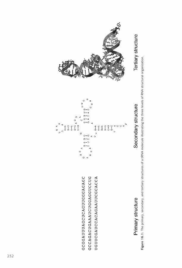
P1: JZP0521840988c16 CB1022/Xiong 0 521 84098 8 January 10, 2006 14:16
Figu
re1
6.1
:Th
epri
mar
y,se
cond
ary,
and
tert
iary
stru
ctur
esof
atR
NA
mol
ecul
eill
ustr
atin
gth
eth
ree
leve
lsof
RN
Ast
ruct
ural
orga
niza
tion
.
232
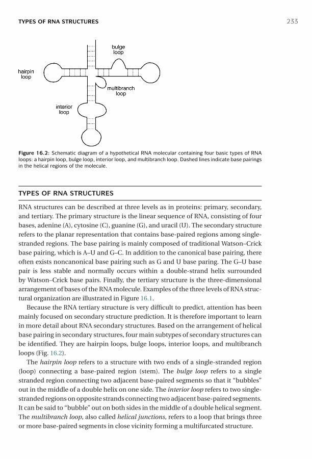
P1: JZP0521840988c16 CB1022/Xiong 0 521 84098 8 January 10, 2006 14:16
TYPES OF RNA STRUCTURES 233
Figure 16.2: Schematic diagram of a hypothetical RNA molecular containing four basic types of RNAloops: a hairpin loop, bulge loop, interior loop, and multibranch loop. Dashed lines indicate base pairingsin the helical regions of the molecule.
TYPES OF RNA STRUCTURES
RNA structures can be described at three levels as in proteins: primary, secondary,and tertiary. The primary structure is the linear sequence of RNA, consisting of fourbases, adenine (A), cytosine (C), guanine (G), and uracil (U). The secondary structurerefers to the planar representation that contains base-paired regions among single-stranded regions. The base pairing is mainly composed of traditional Watson–Crickbase pairing, which is A–U and G–C. In addition to the canonical base pairing, thereoften exists noncanonical base pairing such as G and U base paring. The G–U basepair is less stable and normally occurs within a double-strand helix surroundedby Watson–Crick base pairs. Finally, the tertiary structure is the three-dimensionalarrangement of bases of the RNA molecule. Examples of the three levels of RNA struc-tural organization are illustrated in Figure 16.1.
Because the RNA tertiary structure is very difficult to predict, attention has beenmainly focused on secondary structure prediction. It is therefore important to learnin more detail about RNA secondary structures. Based on the arrangement of helicalbase pairing in secondary structures, four main subtypes of secondary structures canbe identified. They are hairpin loops, bulge loops, interior loops, and multibranchloops (Fig. 16.2).
The hairpin loop refers to a structure with two ends of a single-stranded region(loop) connecting a base-paired region (stem). The bulge loop refers to a singlestranded region connecting two adjacent base-paired segments so that it “bubbles”out in the middle of a double helix on one side. The interior loop refers to two single-stranded regions on opposite strands connecting two adjacent base-paired segments.It can be said to “bubble” out on both sides in the middle of a double helical segment.The multibranch loop, also called helical junctions, refers to a loop that brings threeor more base-paired segments in close vicinity forming a multifurcated structure.

P1: JZP0521840988c16 CB1022/Xiong 0 521 84098 8 January 10, 2006 14:16
234 RNA STRUCTURE PREDICTION
Figure 16.3: A hypothetical RNA structure containing a pseudoknot, kissing hairpin, and hairpin–bulgecontact.
In addition to the traditional secondary structural elements, base pairing betweenloops of different secondary structural elements can result in a higher level of struc-tures such as pseudoknots, kissing hairpins, and hairpin–bulge contact (Fig. 16.3). Apseudoknot loop refers to base pairing formed between loop residues within a hair-pin loop and residues outside the hairpin loop. A kissing hairpin refers to a hydro-gen bonded interaction formed between loop residues of two hairpin structures. Thehairpin–bulge contact refers to interactions between loop residues of a hairpin loopand a bulge loop. This type of interaction forms supersecondary structures, which arerelatively rare in real structures and thus are ignored by most conventional predictionalgorithms.
RNA SECONDARY STRUCTURE PREDICTION METHODS
At present, there are essentially two types of method of RNA structure prediction.One is based on the calculation of the minimum free energy of the stable structurederived from a single RNA sequence. This can be considered an ab initio approach. Thesecond is a comparative approach which infers structures based on an evolutionarycomparison of multiple related RNA sequences.
AB INITIO APPROACH
This approach makes structural predictions based on a single RNA sequence. Therationale behind this method is that the structure of an RNA molecule is solely deter-mined by its sequence. Thus, algorithms can be designed to search for a stable RNAstructure with the lowest free energy. Generally, when a base pairing is formed, theenergy of the molecule is lowered because of attractive interactions between the twostrands. Thus, to search for a most stable structure, ab initio programs are designedto search for a structure with the maximum number of base pairs.
Free energy can be calculated based on parameters empirically derived for smallmolecules. G–C base pairs are more stable than A–U base pairs, which are more stablethan G–U base pairs. It is also known that base-pair formation is not an independentevent. The energy necessary to form individual base pairs is influenced by adjacentbase pairs through helical stacking forces. This is known as cooperativity in helixformation. If a base pair is next to other base pairs, the base pairs tend to stabilize
P1: JZP0521840988c16 CB1022/Xiong 0 521 84098 8 January 10, 2006 14:16
AB INITIO APPROACH 235
each other through attractive stacking interactions between aromatic rings of the basepairs. The attractive interactions lead to even lower energy. Parameters for calculatingthe cooperativity of the base-pair formation have been determined and can be usedfor structure prediction.
However, if the base pair is adjacent to loops or bulges, the neighboring loopsand bulges tend to destabilize the base-pair formation. This is because there is aloss of entropy when the ends of the helical structure are constrained by unpairedloop residues. The destabilizing force to a helical structure also depends on thetypes of loops nearby. Parameters for calculating different destabilizing energieshave also been determined and can be used as penalties for secondary structurecalculations.
The scoring scheme based on the combined stabilizing and destabilizing inter-actions forms the foundation of the ab initio RNA secondary structure predictionmethod. This method works by first finding all possible base-pairing patterns from asequence and then calculating the total energy of a potential secondary structure bytaking into account all the adjacent stabilizing and destabilizing forces. If there aremultiple alternative secondary structures, the method finds the conformation withthe lowest energy, meaning that it is energetically most favorable.
Dot Matrices
In searching for the lowest energy form, all possible base-pair patterns have to beexamined. There are several methods for finding all the possible base-paired regionsfrom a given nucleic acid sequence. The dot matrix method and the dynamic program-ming method introduced in Chapter 3 can be used in detecting self-complementaryregions of a sequence. A simple dot matrix can find all possible base-paring patterns ofan RNA sequence when one sequence is compared with itself (Fig. 16.4). In this case,dots are placed in the matrix to represent matching complementary bases instead ofidentical ones.
The diagonals perpendicular to the main diagonal represent regions that can self-hybridize to form double-stranded structure with traditional A–U and G–C base pairs.In reality, the pattern detection in a dot matrix is often obscured by high noise levels.As discussed in Chapter 3, one way to reduce the noise in the matrix is to selectan appropriate window size of a minimum number of contiguous base matches.Normally, only a window size of four consecutive base matches is used. If the dot plotreveals more than one feasible structures, the lowest energy one is chosen.
Dynamic Programming
The use of a dot plot can be effective in finding a single secondary structure in a smallmolecule (see Fig. 16.4). However, if a large molecule contains multiple secondarystructure segments, choosing a combination that is energetically most stable amonga large number of possibilities can be a daunting task. To overcome the problem,a quantitative approach such as dynamic programming can be used to assemble afinal structure with optimal base-paired regions. In this approach, an RNA sequence
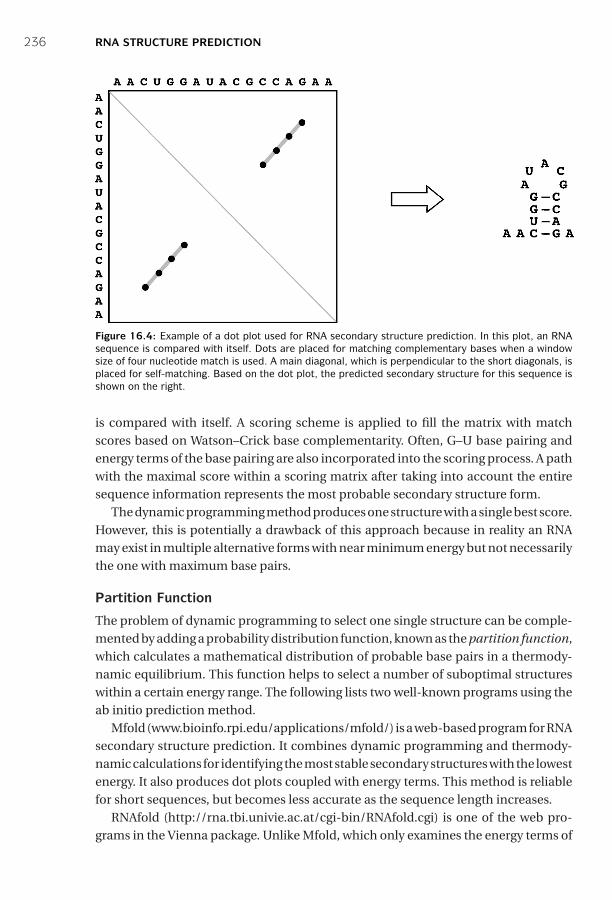
P1: JZP0521840988c16 CB1022/Xiong 0 521 84098 8 January 10, 2006 14:16
236 RNA STRUCTURE PREDICTION
Figure 16.4: Example of a dot plot used for RNA secondary structure prediction. In this plot, an RNAsequence is compared with itself. Dots are placed for matching complementary bases when a windowsize of four nucleotide match is used. A main diagonal, which is perpendicular to the short diagonals, isplaced for self-matching. Based on the dot plot, the predicted secondary structure for this sequence isshown on the right.
is compared with itself. A scoring scheme is applied to fill the matrix with matchscores based on Watson–Crick base complementarity. Often, G–U base pairing andenergy terms of the base pairing are also incorporated into the scoring process. A pathwith the maximal score within a scoring matrix after taking into account the entiresequence information represents the most probable secondary structure form.
The dynamic programming method produces one structure with a single best score.However, this is potentially a drawback of this approach because in reality an RNAmay exist in multiple alternative forms with near minimum energy but not necessarilythe one with maximum base pairs.
Partition Function
The problem of dynamic programming to select one single structure can be comple-mented by adding a probability distribution function, known as the partition function,which calculates a mathematical distribution of probable base pairs in a thermody-namic equilibrium. This function helps to select a number of suboptimal structureswithin a certain energy range. The following lists two well-known programs using theab initio prediction method.
Mfold (www.bioinfo.rpi.edu/applications/mfold/) is a web-based program for RNAsecondary structure prediction. It combines dynamic programming and thermody-namic calculations for identifying the most stable secondary structures with the lowestenergy. It also produces dot plots coupled with energy terms. This method is reliablefor short sequences, but becomes less accurate as the sequence length increases.
RNAfold (http://rna.tbi.univie.ac.at/cgi-bin/RNAfold.cgi) is one of the web pro-grams in the Vienna package. Unlike Mfold, which only examines the energy terms of
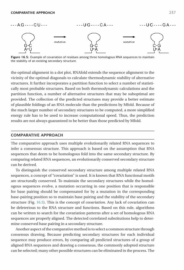
P1: JZP0521840988c16 CB1022/Xiong 0 521 84098 8 January 10, 2006 14:16
COMPARATIVE APPROACH 237
Figure 16.5: Example of covariation of residues among three homologous RNA sequences to maintainthe stability of an existing secondary structure.
the optimal alignment in a dot plot, RNAfold extends the sequence alignment to thevicinity of the optimal diagonals to calculate thermodynamic stability of alternativestructures. It further incorporates a partition function to select a number of statisti-cally most probable structures. Based on both thermodynamic calculations and thepartition function, a number of alternative structures that may be suboptimal areprovided. The collection of the predicted structures may provide a better estimateof plausible foldings of an RNA molecule than the predictions by Mfold. Because ofthe much larger number of secondary structures to be computed, a more simplifiedenergy rule has to be used to increase computational speed. Thus, the predictionresults are not always guaranteed to be better than those predicted by Mfold.
COMPARATIVE APPROACH
The comparative approach uses multiple evolutionarily related RNA sequences toinfer a consensus structure. This approach is based on the assumption that RNAsequences that deem to be homologous fold into the same secondary structure. Bycomparing related RNA sequences, an evolutionarily conserved secondary structurecan be derived.
To distinguish the conserved secondary structure among multiple related RNAsequences, a concept of “covariation” is used. It is known that RNA functional motifsare structurally conserved. To maintain the secondary structures while the homol-ogous sequences evolve, a mutation occurring in one position that is responsiblefor base pairing should be compensated for by a mutation in the correspondingbase-pairing position so to maintain base pairing and the stability of the secondarystructure (Fig. 16.5). This is the concept of covariation. Any lack of covariation canbe deleterious to the RNA structure and functions. Based on this rule, algorithmscan be written to search for the covariation patterns after a set of homologous RNAsequences are properly aligned. The detected correlated substitutions help to deter-mine conserved base pairing in a secondary structure.
Another aspect of the comparative method is to select a common structure throughconsensus drawing. Because predicting secondary structures for each individualsequence may produce errors, by comparing all predicted structures of a group ofaligned RNA sequences and drawing a consensus, the commonly adopted structurecan be selected; many other possible structures can be eliminated in the process. The
P1: JZP0521840988c16 CB1022/Xiong 0 521 84098 8 January 10, 2006 14:16
238 RNA STRUCTURE PREDICTION
comparative-based algorithms can be further divided into two categories based onthe type of input data. One requires predefined alignment and the other does not.
Algorithms That Use Prealignment
This type of algorithm requires the user to provide a pairwise or multiple alignment asinput. The sequence alignment can be obtained using standard alignment programssuch as T-Coffee, PRRN, or Clustal (see Chapter 5). Based on the alignment input,the prediction programs compute structurally consistent mutational patterns suchas covariation and derive a consensus structure common for all the sequences. Inpractice, the consensus structure prediction is often combined with thermodynamiccalculations to improve accuracy.
This type of program is relatively successful for reasonably conserved sequences.The requirement for using this type of program is an appropriate set of homologoussequences that have to be similar enough to allow accurate alignment, but diver-gent enough to allow covariations to be detected. If this condition is not met, correctstructures cannot be inferred. The method also depends on the quality of the inputalignment. If there are errors in the alignment, covariation signals will not be detected.The selection of one single consensus structure is also a drawback because alterna-tive and evolutionarily unconserved structures are not predicted. The following is anexample of this type of program based on predefined aligned sequences.
RNAalifold (http://rna.tbi.univie.ac.at/cgi-bin/alifold.cgi) is a program in theVienna package. It uses a multiple sequence alignment as input to analyze covari-ation patterns on the sequences. A scoring matrix is created that combines minimumfree energy and covariation information. Dynamic programming is used to select thestructure that has the minimum energy for the whole set of aligned RNA sequences.
Algorithms That Do Not Use Prealignment
This type of algorithm simultaneously aligns multiple input sequences and infers aconsensus structure. The alignment is produced using dynamic programming witha scoring scheme that incorporates sequence similarity as well as energy terms.Because the full dynamic programming for multiple alignment is computationallytoo demanding, currently available programs limit the input to two sequences.
Foldalign (http://foldalign.kvl.dk/server/index.html) is a web-based program forRNA alignment and structure prediction. The user provides a pair of unalignedsequences. The program uses a combination of Clustal and dynamic programmingwith a scoring scheme that includes covariation information to construct the align-ment. A commonly conserved structure for both sequences is subsequently derivedbased on the alignment. To reduce computational complexity, the program ignoresmultibranch loops and is only suitable for handling short RNA sequences.
Dynalign (http://rna.urmc.rochester.edu/) is a UNIX program with a free sourcecode for downloading. The user again provides two input sequences. The programcalculates the possible secondary structures of each using a method similar to Mfold.

P1: JZP0521840988c16 CB1022/Xiong 0 521 84098 8 January 10, 2006 14:16
SUMMARY 239
By comparing multiple alternative structures from each sequence, a lowest energystructure common to both sequences is selected that serves as the basis for sequencealignment. The unique feature of this program is that it does not require sequencesimilarity and therefore can handle very divergent sequences. However, because ofthe computation complexity, the program only predicts small RNA sequences such astRNA with reasonable accuracy.
PERFORMANCE EVALUATION
Rigorously evaluating the performance of RNA prediction programs has traditionallybeen hindered by the dearth of three-dimensional structural information for RNA.The availability of recently solved crystal structures of the entire ribosome providesa wealth of structural details relating to diverse types of RNA molecules. The high-resolution structural information can then be used as a benchmark for evaluatingstate-of-the-art RNA structure prediction programs in all categories.
If prediction accuracy can be represented using a single parameter such as the cor-relation coefficient, which takes into account both sensitivity and selectivity informa-tion (see Chapter 8), the ab initio–based programs score roughly 20% to 60% depend-ing on the length of the sequences. Generally speaking, the programs perform betterfor shorter RNA sequences than for longer ones. For small RNA sequences, such astRNA, some programs may be able to produce 70% accuracy. The major limitation forperformance gains of this category appears to be dependence on energy parametersalone, which may not be sufficient to distinguish different structural possibilities ofthe same molecule.
Based on recent benchmark comparisons, the comparative-type algorithms canreach an accuracy range of 20% to 80%. The results depend on whether a pro-gram is prealignment dependent or not. Most of the superior performance comesfrom prealignment-dependent programs such as RNAalifold. The prealignment-independent programs fare much worse for predicting long sequences. For smallRNA sequences such as tRNA, both subtypes can achieve very high accuracy (up to100%). This illustrates that the comparative approach is consistently more accuratethan the ab initio one.
SUMMARY
Detailed understanding of RNA structures is important for understanding the func-tional role of RNA in the cell. The demand for structural information about RNA hasmotivated the development of a large number of prediction algorithms. Current RNAstructure prediction is predominantly focused on secondary structures owing to thedifficulty in predicting tertiary structures. The secondary structure prediction meth-ods can be classified as either ab initio or comparative. The ab initio method is basedon energetic calculations from a single query sequence. However, the accuracy ofthe ab initio method is limited. The comparative approach, which requires multiple
P1: JZP0521840988c16 CB1022/Xiong 0 521 84098 8 January 10, 2006 14:16
240 RNA STRUCTURE PREDICTION
sequences, is able to achieve better accuracy. However, the obvious drawback of theconsensus approach is the requirement for a unique set of homologous sequences.Neither type of the prediction methods currently considers pseudoknots in the RNAstructure because of the much greater computational complexity involved. To fur-ther increase prediction performance, the research and development should focuson alleviating some of the current drawbacks.
FURTHER READING
Doshi, K. J., Cannone, J. J., Cobaugh, C. W., and Gutell, R. R. 2004. Evaluation of the suitabilityof free-energy minimization using nearest-neighbor energy parameters for RNA secondarystructure prediction. BMC Bioinformatics 5:105.
Doudna, J. A. 2000. Structural genomics of RNA. Nat. Struct. Biol. Suppl:954–6.Gardner, P. P., and Giegerich, R. 2004. A comprehensive comparison of comparative RNA struc-
ture prediction approaches. BMC Bioinformatics 5:140.Gorodkin, J. Stricklin, S. L., and Stormo, G. D. 2001. Discovering common stem-loop motifs in
unaligned RNA sequences. Nucleic Acids. Res. 10:2135–44.Leontis, N. B., Stombaugh, J., and Westhof, E. 2002. Motif prediction in ribosomal RNAs lessons
and prospects for automated motif prediction in homologous RNA molecules. Biochimie84:961–73.
Major, F., and Griffey, R. 2001. Computational methods for RNA structure determination. Curr.Opin. Struct. Biol. 11:282–6.
Westhof, E., Auffinger, P., and Gaspin, C. 1997. “DNA and RNA structure prediction.: In: DNAand Protein Sequence Analysis, edited by M. J. Bishop and C. J. Rawlings, 255–78. Oxford, UK:IRL Press.

P1: JZP0521840988c17 CB1022/Xiong 0 521 84098 8 January 10, 2006 11:58
SECTION SIX
Genomics and Proteomics
241

P1: JZP0521840988c17 CB1022/Xiong 0 521 84098 8 January 10, 2006 11:58
242

P1: JZP0521840988c17 CB1022/Xiong 0 521 84098 8 January 10, 2006 11:58
CHAPTER SEVENTEEN
Genome Mapping, Assembly, and Comparison
Genomics is the study of genomes. Genomic studies are characterized by simultane-ous analysis of a large number of genes using automated data gathering tools. Thetopics of genomics range from genome mapping, sequencing, and functional genomicanalysis to comparative genomic analysis. The advent of genomics and the ensuingexplosion of sequence information are the main driving force behind the rapid devel-opment of bioinformatics today.
Genomic study can be tentatively divided into structural genomics and functionalgenomics. Structural genomics refers to the initial phase of genome analysis, whichincludes construction of genetic and physical maps of a genome, identification ofgenes, annotation of gene features, and comparison of genome structures. This is themajor theme of discussion of this chapter. However, it should to be mentioned thatthe term structural genomics has already been used by a structural biology group foran initiative to determine three-dimensional structures of all proteins in a cell. Strictlyspeaking, the initiative of structural determination of proteins falls within the realmof structural proteomics and should not be confused as a subdiscipline of genomics.The structure genomics discussed herein mainly deals with structures of genomesequences. Functional genomics refers to the analysis of global gene expression andgene functions in a genome, which is discussed in Chapter 18.
GENOME MAPPING
The first step to understanding a genome structure is through genome mapping,which is a process of identifying relative locations of genes, mutations or traits ona chromosome. A low-resolution approach to mapping genomes is to describe theorder and relative distances of genetic markers on a chromosome. Genetic markers areidentifiable portions of a chromosome whose inheritance patterns can be followed.For many eukaryotes, genetic markers represent morphologic phenotypes. In additionto genetic linkage maps, there are also other types of genome maps such as physicalmaps and cytologic maps, which describe genomes at different levels of resolution.Their relations relative to the DNA sequence on a chromosome are illustrated inFigure 17.1. More details of each type of genome maps are discussed next.
Genetic linkage maps, also called genetic maps, identify the relative positions ofgenetic markers on a chromosome and are based on how frequent the markers areinherited together. The rationale behind genetic mapping is that the closer the two
243

P1: JZP0521840988c17 CB1022/Xiong 0 521 84098 8 January 10, 2006 11:58
244 GENOME MAPPING, ASSEMBLY, AND COMPARISON
Figure 17.1: Overview of various genome maps relative to the genomic DNA sequence. The mapsrepresent different levels of resolution to describe a genome using genetic markers. Cytologic maps areobtained microscopically. Genetic maps (grey bar) are obtained through genetic crossing experiments inwhich chromosome recombinations are analyzed. Physical maps are obtained from overlapping clonesidentified by hybridizing the clone fragments (grey bars) with common probes (grey asterisks).
genetic markers are, the more likely it is that they are inherited together and are notseparated in a genetic crossing event. The distance between the two genetic markersis measured in centiMorgans (cM), which is the frequency of recombination of geneticmarkers. One centiMorgan is defined as one percentage of the total recombinationevents when separation of the two genetic markers is observed in a genetic cross-ing experiment. One centiMorgan is approximately 1 Mb in humans and 0.5 Mb inDrosophila.
Physical maps are maps of locations of identifiable landmarks on a genomic DNAregardless of inheritance patterns. The distance between genetic markers is measureddirectly as kilobases (Kb) or megabases (Mb). Because the distance is expressed inphysical units, it is more accurate and reliable than centiMorgans used in geneticmaps. Physical maps are constructed by using a chromosome walking technique,which uses a number of radiolabeled probes to hybridize to a library of DNA clonefragments. By identifying overlapping clones probed by common probes, a relativeorder of the cloned fragments can be established.
Cytologic maps refer to banding patterns seen on stained chromosomes, whichcan be directly observed under a microscope. The observable light and dark bandsare the visually distinct markers on a chromosome. A genetic marker can be asso-ciated with a specific chromosomal band or region. The banding patterns, how-ever, are not always constant and are subject to change depending on the extent
P1: JZP0521840988c17 CB1022/Xiong 0 521 84098 8 January 10, 2006 11:58
GENOME SEQUENCING 245
of chromosomal contraction. Thus, cytologic maps can be considered to be of verylow resolution and hence somewhat inaccurate physical maps. The distance betweentwo bands is expressed in relative units (Dustin units).
GENOME SEQUENCING
The highest resolution genome map is the genomic DNA sequence that can be con-sidered as a type of physical map describing a genome at the single base-pair level.DNA sequencing is now routinely carried out using the Sanger method. This involvesthe use of DNA polymerases to synthesize DNA chains of varying lengths. TheDNA synthesis is stopped by adding dideoxynucleotides. The dideoxynucleotides arelabeled with fluorescent dyes, which terminate the DNA synthesis at positions con-taining all four bases, resulting in nested fragments that vary in length by a singlebase. When the labeled DNA is subjected to electrophoresis, the banding patterns inthe gel reveal the DNA sequence.
The fluorescent traces of the DNA sequences are read by a computer program thatassigns bases for each peak in a chromatogram. This process is called base calling.Automated base calling may generate errors and human intervention is often requiredto correct the sequence calls.
There are two major strategies for whole genome sequencing: the shotgunapproach and the hierarchical approach. The shotgun approach randomly sequencesclones from both ends of cloned DNA. This approach generates a large number ofsequenced DNA fragments. The number of random fragments has to be very large,so large that the DNA fragments overlap sufficiently to cover the entire genome.This approach does not require knowledge of physical mapping of the clone frag-ments, but rather a robust computer assembly program to join the pieces of randomfragments into a single, whole-genome sequence. Generally, the genome has to beredundantly sequenced in such a way that the overall length of the fragments coversthe entire genome multiple times. This is designed to minimize sequencing errorsand ensure correct assembly of a contiguous sequence. Overlapping sequences withan overall length of six to ten times the genome size are normally obtained for thispurpose.
Despite the multiple coverage, sometimes certain genomic regions remainunsequenced, mainly owing to cloning difficulties. In such cases, the remain-der gap sequences can be obtained through extending sequences from regions ofknown genomic sequences using a more traditional PCR technique, which requiresthe use of custom primers and performs genome walking in a stepwise fash-ion. This step of genome sequencing is also known as finishing, which is fol-lowed by computational assembly of all the sequence data into a final completegenome.
The hierarchical genome sequencing approach is similar to the shotgun approach,but on a smaller scale. The chromosomes are initially mapped using the physicalmapping strategy. Longer fragments of genomic DNA (100 to 300 kB) are obtained
P1: JZP0521840988c17 CB1022/Xiong 0 521 84098 8 January 10, 2006 11:58
246 GENOME MAPPING, ASSEMBLY, AND COMPARISON
and cloned into a high-capacity bacterial vector called bacterial artificial chromo-some (BAC). Based on the results of physical mapping, the locations and orders of theBAC clones on a chromosome can be determined. By successively sequencing adja-cent BAC clone fragments, the entire genome can be covered. The complete sequenceof each individual BAC clone can be obtained using the shotgun approach. Overlap-ping BAC clones are subsequently assembled into an entire genome sequence. Majordifferences between the hierarchical and the full shotgun approaches are shown inFigure 17.2.
During the era of human genome sequencing, there was a heated debate on themerits of each of the two strategies. In fact, there are advantages and disadvantagesin either. The hierarchical approach is slower and more costly than the shotgunapproach because it involves an initial clone-based physical mapping step. However,once the map is generated, assembly of the whole genome becomes relatively easyand less error prone. In contrast, the whole genome shotgun approach can producea draft sequence very rapidly because it is based on the direct sequencing approach.However, it is computationally very demanding to assemble the short random frag-ments. Although the approach has been successfully employed in sequencing smallmicrobial genomes, for a complex eukaryotic genome that contains high levels ofrepetitive sequences, such as the human genome, the full shotgun approach becomesless accurate and tends to leave more “holes” in the final assembled sequence thanthe hierarchical approach. Current genome sequencing of large organisms often usesa combination of both approaches.
GENOME SEQUENCE ASSEMBLY
As described, initial DNA sequencing reactions generate short sequence reads fromDNA clones. The average length of the reads is about 500 bases. To assemble a wholegenome sequence, these short fragments are joined to form larger fragments afterremoving overlaps. These longer, merged sequences are termed contigs, which areusually 5,000 to 10,000 bases long. A number of overlapping contigs can be furthermerged to form scaffolds (30,000–50,000 bases, also called supercontigs), which areunidirectionally oriented along a physical map of a chromosome (Fig. 17.3). Overlap-ping scaffolds are then connected to create the final highest resolution map of thegenome.
Correct identification of overlaps and assembly of the sequence reads into contigsare like joining jigsaw puzzles, which can be very computationally intensive whendealing with data at the whole-genome level. The major challenges in genome assem-bly are sequence errors, contamination by bacterial vectors, and repetitive sequenceregions. Sequence errors can often be corrected by drawing a consensus from an align-ment of multiple overlapped sequences. Bacterial vector sequences can be removedusing filtering programs prior to assembly. To overcome the problem of sequencerepeats, programs such as RepeatMasker (see Chapter 4) can be used to detect and
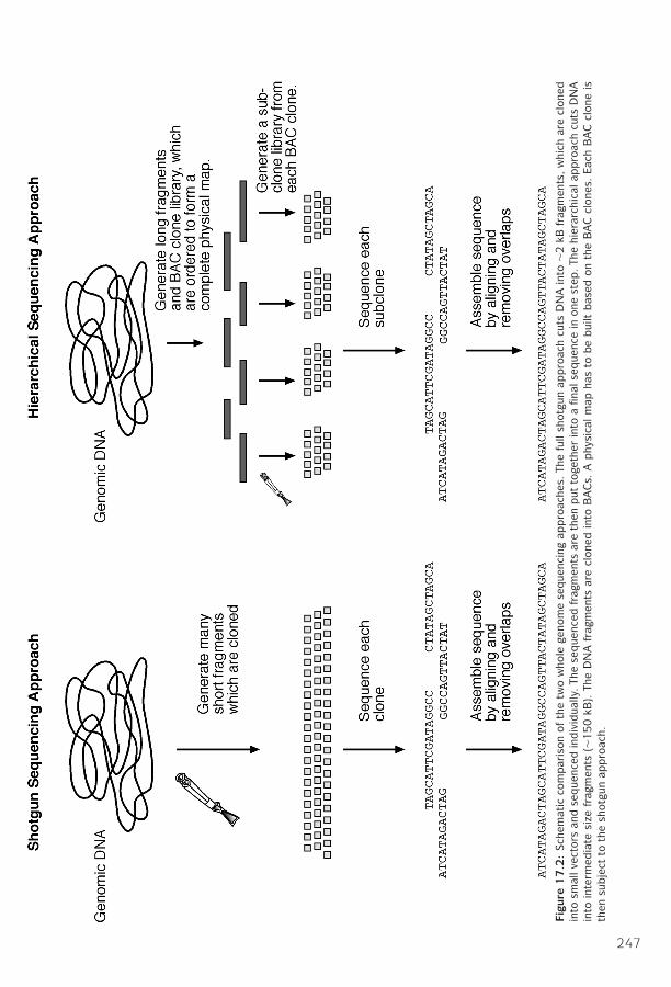
P1: JZP0521840988c17 CB1022/Xiong 0 521 84098 8 January 10, 2006 11:58
Figu
re1
7.2
:Sch
emat
icco
mpar
ison
ofth
etw
ow
hole
geno
me
seque
ncin
gap
pro
ache
s.Th
efu
llsh
otgu
nap
pro
ach
cuts
DN
Ain
to∼2
kBfr
agm
ents
,w
hich
are
clon
edin
tosm
allv
ecto
rsan
dse
que
nced
indiv
idua
lly.Th
ese
que
nced
frag
men
tsar
eth
enput
toge
ther
into
afin
alse
que
nce
inon
est
ep.Th
ehi
erar
chic
alap
pro
ach
cuts
DN
Ain
toin
term
edia
tesi
zefr
agm
ents
(∼150
kB).
The
DN
Afr
agm
ents
are
clon
edin
toB
AC
s.A
phy
sica
lm
apha
sto
be
bui
ltbas
edon
the
BA
Ccl
ones
.Ea
chB
AC
clon
eis
then
subje
ctto
the
shot
gun
appro
ach.
247
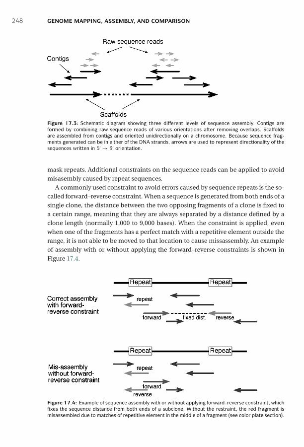
P1: JZP0521840988c17 CB1022/Xiong 0 521 84098 8 January 10, 2006 11:58
248 GENOME MAPPING, ASSEMBLY, AND COMPARISON
Figure 17.3: Schematic diagram showing three different levels of sequence assembly. Contigs areformed by combining raw sequence reads of various orientations after removing overlaps. Scaffoldsare assembled from contigs and oriented unidirectionally on a chromosome. Because sequence frag-ments generated can be in either of the DNA strands, arrows are used to represent directionality of thesequences written in 5′ → 3′ orientation.
mask repeats. Additional constraints on the sequence reads can be applied to avoidmisasembly caused by repeat sequences.
A commonly used constraint to avoid errors caused by sequence repeats is the so-called forward–reverse constraint. When a sequence is generated from both ends of asingle clone, the distance between the two opposing fragments of a clone is fixed toa certain range, meaning that they are always separated by a distance defined by aclone length (normally 1,000 to 9,000 bases). When the constraint is applied, evenwhen one of the fragments has a perfect match with a repetitive element outside therange, it is not able to be moved to that location to cause missassembly. An exampleof assembly with or without applying the forward–reverse constraints is shown inFigure 17.4.
Figure 17.4: Example of sequence assembly with or without applying forward–reverse constraint, whichfixes the sequence distance from both ends of a subclone. Without the restraint, the red fragment ismisassembled due to matches of repetitive element in the middle of a fragment (see color plate section).
P1: JZP0521840988c17 CB1022/Xiong 0 521 84098 8 January 10, 2006 11:58
GENOME SEQUENCE ASSEMBLY 249
Base Calling and Assembly Programs
The first step toward genome assembly is to derive base calls and assign associatedquality scores. The next step is to assemble the sequence reads into contiguoussequences. This step includes identifying overlaps between sequence fragments,assigning the order of the fragments and deriving a consensus of an overall sequence.Assembling all shotgun fragments into a full genome is a computationally very chal-lenging step. There are a variety of programs available for processing the raw sequencedata. The following is a selection of base calling and assembly programs commonlyused in genome sequencing projects.
Phred (www.phrap.org/) is a UNIX program for base calling. It uses a Fourier anal-ysis to resolve fluorescence traces and predict actual peak locations of bases. It alsogives a probability score for each base call that may be attributable to error. The com-monly accepted score threshold is twenty, which corresponds to a 1% chance of error.The higher the score, the better the quality of the sequence reads. If the score valuefalls below the threshold, human intervention is required.
Phrap (www.phrap.org/) is a UNIX program for sequence assembly. It takes Phredbase-call files with quality scores as input and aligns individual fragments in apairwise fashion using the Smith–Waterman algorithm. The base quality informa-tion is taken into account during the pairwise alignment. After all the pairwisesequence similarity is identified, the program performs assembly by progressivelymerging sequence pairs with decreasing similarity scores while removing over-lapped regions. Consensus contigs are derived after joining all possible overlappedreads.
VecScreen (www.ncbi.nlm.nih.gov/VecScreen/VecScreen.html) is a web-basedprogram that helps detect contaminating bacterial vector sequences. It scans an inputnucleotide sequence and compares it with a database of known vector sequences byusing the BLAST program.
TIGR Assembler (www.tigr.org/) is a UNIX program from TIGR for assembly oflarge shotgun sequence fragments. It treats the sequence input as clean reads withoutconsideration of the sequence quality. A main feature of the program is the appli-cation of the forward–reverse constraints to avoid misassembly caused by sequencerepeats. The sequence alignment in the assembly stage is performed using the Smith–Waterman algorithm.
ARACHNE (www-genome.wi.mit.edu/wga/) is a free UNIX program for the assem-bly of whole-genome shotgun reads. Its unique features include using a heuristicapproach similar to FASTA to align overlapping fragments, evaluating alignmentsusing statistical scores, correcting sequencing errors based on multiple sequencealignment, and using forward–reverse constraints. It accepts base calls with asso-ciated quality scores assigned by Phred as input and produces scaffolds or a fullyassembled genome.
EULER (http://nbcr.sdsc.edu/euler/) is an assembly algorithm that uses a EulerianSuperpath approach, which is a polynomial algorithm for solving puzzles such as thefamous “traveling salesman problem”: finding the shortest path of visiting a given
P1: JZP0521840988c17 CB1022/Xiong 0 521 84098 8 January 10, 2006 11:58
250 GENOME MAPPING, ASSEMBLY, AND COMPARISON
number of cities exactly once and returning to the starting point. In this approach,a sequence fragment is broken down to tuples of twenty nucleotides. The tuplesare distributed in a diagram with numerous nodes that are all interconnected. Thetuples are converted to binary vectors in the nodes. By using a Viterbi algorithm (seeChapter 6), the shortest path among the vectors can be found, which is the best way toconnect the tuples into a full sequence. Because this approach does not directly relyon detecting overlaps, it may be advantageous in assembling sequences with repeatmotifs.
GENOME ANNOTATION
Before the assembled sequence is deposited into a database, it has to be analyzedfor useful biological features. The genome annotation process provides commentsfor the features. This involves two steps: gene prediction and functional assignment.Some examples of finished gene annotations in GenBank have been described in theBiological Database section (see Chapter 2). The following example illustrates theoverall process employed in annotating the human genome.
As a real-world example, gene annotation of the human genome employs a com-bination of theoretical prediction and experimental verification. Gene structures arefirst predicted by ab initio exon prediction programs such as GenScan or FgenesH(see Chapter 8). The predictions are verified by BLAST searches against a sequencedatabase. The predicted genes are further compared with experimentally determinedcDNA and EST sequences using the pairwise alignment programs such as GeneWise,Spidey, SIM4, and EST2Genome. All predictions are manually checked by humancurators. Once open reading frames are determined, functional assignment of theencoded proteins is carried out by homology searching using BLAST searches againsta protein database. Further functional descriptions are added by searching proteinmotif and domain databases such as Pfam and InterPro (see Chapter 7) as well as byrelying on published literature.
Gene Ontology
A problem arises when using existing literature because the description of a gene func-tion uses natural language, which is often ambiguous and imprecise. Researchersworking on different organisms tend to apply different terms to the same type ofgenes or proteins. Alternatively, the same terminology used in different organismsmay actually refer to different genes or proteins. Therefore, there is a need to stan-dardize protein functional descriptions. This demand has spurred the developmentof the gene ontology (GO) project, which uses a limited vocabulary to describemolecular functions, biological processes, and cellular components. The controlledvocabulary is organized such that a protein function is linked to the cellular func-tion through a hierarchy of descriptions with increasing specificity. The top of thehierarchy provides an overall picture of the functional class, whereas the lower level
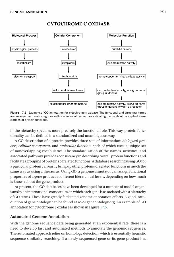
P1: JZP0521840988c17 CB1022/Xiong 0 521 84098 8 January 10, 2006 11:58
GENOME ANNOTATION 251
Figure 17.5: Example of GO annotation for cytochrome c oxidase. The functional and structural termsare arranged in three categories with a number of hierarchies indicating the levels of conceptual asso-ciations of protein functions.
in the hierarchy specifies more precisely the functional role. This way, protein func-tionality can be defined in a standardized and unambiguous way.
A GO description of a protein provides three sets of information: biological pro-cess, cellular component, and molecular function, each of which uses a unique setof nonoverlapping vocabularies. The standardization of the names, activities, andassociated pathways provides consistency in describing overall protein functions andfacilitates grouping of proteins of related functions. A database searching using GO fora particular protein can easily bring up other proteins of related functions in much thesame way as using a thesaurus. Using GO, a genome annotator can assign functionalproperties of a gene product at different hierarchical levels, depending on how muchis known about the gene product.
At present, the GO databases have been developed for a number of model organ-isms by an international consortium, in which each gene is associated with a hierarchyof GO terms. These have greatly facilitated genome annotation efforts. A good intro-duction of gene ontology can be found at www.geneontology.org. An example of GOannotation for cytochrome c oxidase is shown in Figure 17.5.
Automated Genome Annotation
With the genome sequence data being generated at an exponential rate, there is aneed to develop fast and automated methods to annotate the genomic sequences.The automated approach relies on homology detection, which is essentially heuristicsequence similarity searching. If a newly sequenced gene or its gene product has

P1: JZP0521840988c17 CB1022/Xiong 0 521 84098 8 January 10, 2006 11:58
252 GENOME MAPPING, ASSEMBLY, AND COMPARISON
significant matches with a database sequence beyond a certain threshold, a transferof functional assignment is taking place. In addition to sequence matching at the fulllength, detection of conserved motifs often offers additional functional clues.
Because using a single database searching method is often incomplete and errorprone, automated methods have to mimic the manual process, which takes intoconsideration multiple lines of evidence in assigning a gene function, to minimizeerrors. The following algorithm is an example that goes a step beyond examiningsequence similarity and provides functional annotations based on multiple proteincharacteristics.
GeneQuiz (http://jura.ebi.ac.uk:8765/ext-genequiz/) is a web server for proteinsequence annotation. The program compares a query sequence against databasesusing BLAST and FASTA to identify homologs with high similarities. In addition, itperforms domain analysis using the PROSITE and Blocks databases (see Chapter 7) aswell as analysis of secondary structures and supersecondary structures that includesprediction of coiled coils and transmembrane helices. Multiple search and analysisresults are compiled to produce a summary of protein function with an assignedconfidence level (clear, tentative, marginal, and negligible).
Annotation of Hypothetical Proteins
Although a large number of genes and proteins can be assigned functions by thesequence similarity based approach, about 40% of the genes from newly sequencedgenomes have no known functions and can only be annotated as genes encoding“hypothetical proteins.” Experimental discovery of the functions of these genes andproteins is often time consuming and difficult because of lack of hypotheses to designexperiments. In this situation, more advanced tools can be used for functional pre-dictions by searching for remote homologs.
One way to obtain functional hints of genes encoding hypothetical proteins is bysearching for remote homologs in databases. Detecting remote homologs typicallyinvolves combined searches of protein motifs and domains and prediction for sec-ondary and tertiary structures. Conserved functional sites can be identified by profileand hidden Markov model–based motif and domain search tools such as SMART andInterPro (see Chapter 7). The prediction can also be performed using structure-basedapproaches such as threading and fold recognition (see Chapter 15). If the distanthomologs detected using the structural approach are linked with well-defined func-tions, a broad functional class of the query protein if not the precise function of theprotein can be inferred. In addition, prediction results for subcellular localization,protein–protein interactions can provide further functional hints (see Chapter 19).
These suggestions do not guarantee to provide correct annotations for the “hypo-thetical proteins,” but they may provide critical hypotheses of the protein functionthat can be tested in the laboratory. The remote homology detection helps to shedlight on the possible functions of the proteins that previously have no functionalinformation at all. Thus, the bioinformatic analysis can spur an important advancein knowledge in many cases. Some hypothetical proteins, because of their novel
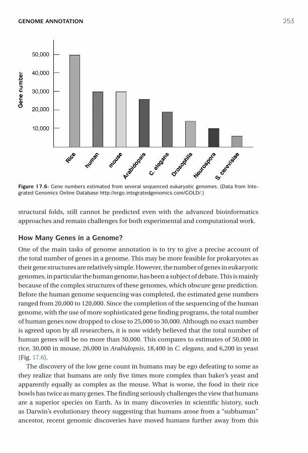
P1: JZP0521840988c17 CB1022/Xiong 0 521 84098 8 January 10, 2006 11:58
GENOME ANNOTATION 253
Figure 17.6: Gene numbers estimated from several sequenced eukaryotic genomes. (Data from Inte-grated Genomics Online Database http://ergo.integratedgenomics.com/GOLD/.)
structural folds, still cannot be predicted even with the advanced bioinformaticsapproaches and remain challenges for both experimental and computational work.
How Many Genes in a Genome?
One of the main tasks of genome annotation is to try to give a precise account ofthe total number of genes in a genome. This may be more feasible for prokaryotes astheir gene structures are relatively simple. However, the number of genes in eukaryoticgenomes, in particular the human genome, has been a subject of debate. This is mainlybecause of the complex structures of these genomes, which obscure gene prediction.Before the human genome sequencing was completed, the estimated gene numbersranged from 20,000 to 120,000. Since the completion of the sequencing of the humangenome, with the use of more sophisticated gene finding programs, the total numberof human genes now dropped to close to 25,000 to 30,000. Although no exact numberis agreed upon by all researchers, it is now widely believed that the total number ofhuman genes will be no more than 30,000. This compares to estimates of 50,000 inrice, 30,000 in mouse, 26,000 in Arabidopsis, 18,400 in C. elegans, and 6,200 in yeast(Fig. 17.6).
The discovery of the low gene count in humans may be ego defeating to some asthey realize that humans are only five times more complex than baker’s yeast andapparently equally as complex as the mouse. What is worse, the food in their ricebowls has twice as many genes. The finding seriously challenges the view that humansare a superior species on Earth. As in many discoveries in scientific history, suchas Darwin’s evolutionary theory suggesting that humans arose from a “subhuman”ancestor, recent genomic discoveries have moved humans further away from this
P1: JZP0521840988c17 CB1022/Xiong 0 521 84098 8 January 10, 2006 11:58
254 GENOME MAPPING, ASSEMBLY, AND COMPARISON
exalted status. However, before we are overwhelmed by the humble realization, weshould also realize that the complexity of an organism simply cannot be representedby gene numbers. As will soon become clear, gene expression and regulation, proteinexpression, modification, and interactions all contribute to the overall complexity ofan organism.
Genome Economy
One level of genetic complexity is manifested at the protein expression level in whichthere are often more expressed proteins than genes available to code for them. Forexample, in humans, there are more than 100,000 proteins expressed based on ESTanalysis (see Chapter 18) compared to no more than 30,000 genes. If the “one gene,one protein” paradigm holds true, how could this discrepancy exist? Where does theextra coding power come from?
The answer lies in “genome economy,” a phenomenon of synthesizing more pro-teins from fewer genes. This is a major strategy that eukaryotic organisms use toachieve a myriad of phenotypic diversities. There are many underlying genetic mech-anisms to help account for genome economy. A major mechanism responsible for theprotein diversity is alternative splicing, which refers to the splicing event that joinsdifferent exons from a single gene to form different transcripts. A related mechanism,known as exon shuffling, which joins exons from different genes to generate more tran-scripts, is also common in eukaryotes. It is known that, in humans, about two thirdsof the genes exhibit alternative splicing and exon shuffling during expression, gener-ating 90% of the total proteins. In Drosophila, the DSCAM gene contains 115 exonsthat can be alternatively spliced to produce 38,000 different proteins. This remarkableability to generate protein diversity and new functions highlights the true complexityof a genome. It also illustrates the evolutionary significance of introns in eukaryoticgenes, which serve as spacers that make the molecular recombination possible.
There are more surprising mechanisms responsible for genome economy. Forexample, trans-splicing can occur between RNAs produced from both DNA strands.In the Drosophila mdg4 mutant, RNA transcribed from four exons in the sense strandand two exons in the antisense strand are joined to form a single mRNA. With dif-ferent exon combinations, four different proteins can be produced. In some circum-stances, one mRNA transcript can lead to the translation of more than one protein.For example, human dentin phosphoprotein and dentin sialoprotein are proteinsinvolved in tooth formation. An mRNA transcript that includes coding regions fromboth proteins is translated into a precursor protein that is cleaved to produce two dif-ferent mature proteins. Another situation, called “gene within gene,” can be found ina gene for human prostate-specific antigen (PSA). In addition to regular PSA, humanscan produce a similar protein, called PSA-LM, that functions antagonistically to PSAand is important for prostate cancer diagnosis. PSA-LM turns out to be encoded bythe fourth intron of the PSA gene.
These are just a few known mechanisms of condensing the coding potential ofgenomic DNA to achieve increased protein diversity. From a bioinformatics point of
P1: JZP0521840988c17 CB1022/Xiong 0 521 84098 8 January 10, 2006 11:58
COMPARATIVE GENOMICS 255
view, this makes gene prediction based on computational approaches all the morecomplicated. It also highlights one of the challenges that faces software programdevelopers today. A number of databases have recently been established to archivealternatively spliced forms of eukaryotic genes. The following is one such example forhuman genes.
ProSplicer (http://prosplicer.mbc.nctu.edu.tw/) is a web-based database of humanalternative spliced transcripts. The spliced variants are identified by aligning eachknown human protein, mRNA, and EST sequence against the genomic sequenceusing the SIM4 and TBLASTN program. The three sets of alignment are compiledto derive alternative splice forms. The database organizes data by tissue types andcan be searched using keywords.
COMPARATIVE GENOMICS
Comparison of whole genomes from different organisms is comparative genomics,which includes comparison of gene number, gene location, and gene content fromthese genomes. The comparison helps to reveal the extent of conservation amonggenomes, which will provide insights into the mechanism of genome evolution andgene transfer among genomes. It helps to understand the pattern of acquisition offoreign genes through lateral gene transfer. It also helps to reveal the core set of genescommon among different genomes, which should correspond to the genes that arecrucial for survival. This knowledge can be potentially useful in future metabolicpathway engineering.
As alluded to previously, the main themes of comparative genomics include wholegenome alignment, comparing gene order between genomes, constructing minimalgenomes, and lateral gene transfer among genomes, each of which is discussed inmore detail.
Whole Genome Alignment
With an ever-increasing number of genome sequences available, it becomes impera-tive to understand sequence conservation between genomes, which often helps toreveal the presence of conserved functional elements. This can be accomplishedthrough direct genome comparison or genome alignment. The alignment at thegenome level is fundamentally no different from the basic sequence alignmentdescribed in Chapters 3, 4, and 5. However, alignment of extremely large sequencespresents new complexities owing to the sheer size of the sequences. Regular alignmentprograms tend to be error prone and inefficient when dealing with long stretches ofDNA containing hundreds or thousands of genes. Another challenge of genome align-ment is effective visualization of alignment results. Because it is obviously difficult tosift through and make sense of the extremely large alignments, a graphical representa-tion is a must for interpretation of the result. Therefore, specific alignment algorithmsare needed to deal with the unique challenges of whole genome alignment. A numberof alignment programs for “super-long” DNA sequences are described next.

P1: JZP0521840988c17 CB1022/Xiong 0 521 84098 8 January 10, 2006 11:58
256 GENOME MAPPING, ASSEMBLY, AND COMPARISON
MUMmer (Maximal Unique Match, www.tigr.org/tigr-scripts/CMR2/webmum/mumplot) is a free UNIX program from TIGR for alignment of two entire genomesequences and comparison of the locations of orthologs. The program is essentially amodified BLAST, which, in the seeding step (see Chapter 4), finds the longest approx-imate matches that include mismatches instead of finding exact k-mer matches asin regular BLAST. The result of the alignment of whole genomes is shown as a dotplot with lines of connected dots to indicate collinearity of genes. It is optimized forpairwise comparison of closely related microbial genomes.
BLASTZ (http://bio.cse.psu.edu/) is a UNIX program modified from BLAST to dopairwise alignment of very large genomic DNA sequences. The modified BLAST pro-gram first masks repetitive sequences and searches for closely matched “words,”which are defined as twelve identical matches within a stretch of nineteen nucleotides.The words serve as seeds for extension of alignment in both directions until the scoresdrop below a certain threshold. Nearby aligned regions are joined by using a weightedscheme that employs a unique gap penalty scheme that tolerates minor variationssuch as transitions in the seeding step of the alignment construction to increase itssensitivity.
LAGAN (Limited Area Global Alignment of Nucleotides; http://lagan.stanford.edu/) is a web-based program designed for pairwise alignment of large genomes. Itfirst finds anchors between two genomic sequences using an algorithm that identifiesshort, exactly matching words. Regions that have high density of words are selected asanchors. The alignments around the anchors are built using the Needleman–Wunschglobal alignment algorithm. Nearby aligned regions are further connected using thesame algorithm. The unique feature of this program is that it is able to take into accountdegeneracy of the genetic codes and is therefore able to handle more distantly relatedgenomes. Multi-LAGAN, an extension of LAGAN, available from the same website,performs multiple alignment of genomes using a progressive approach similar to thatused in Clustal (see Chapter 5).
PipMaker (http://bio.cse.psu.edu/cgi-bin/pipmaker?basic) is a web server usingthe BLASTZ heuristic method to find similar regions in two DNA sequences. It pro-duces a textual output of the alignment result and also a graphical output that presentsthe alignment as a percent identity plot as well as a dot plot. For comparing multiplegenomes, MultiPipMaker is available from the same site.
MAVID (http://baboon.math.berkeley.edu/mavid/) is a web-based program foraligning multiple large DNA sequences. MAVID is based on a progressive alignmentalgorithm similar to Clustal. It produces an NJ tree as a guide tree. The sequences arealigned recursively using a heuristic pairwise alignment program called AVID. AVIDworks by first selecting anchors using the Smith–Waterman algorithm and then build-ing alignments for the sequences between nearby anchors. Connected alignments aretreated as new anchors for building longer alignments. The process is repeated itera-tively until the entire sequence pair including weakly conserved regions are aligned.
GenomeVista (http://pipeline.lbl.gov/cgi-bin/GenomeVista) is a database search-ing program that searches against the human, mouse, rat, or Drosophila genomesusing a large piece of DNA as query. It uses a program called BLAT to find anchors and
P1: JZP0521840988c17 CB1022/Xiong 0 521 84098 8 January 10, 2006 11:58
COMPARATIVE GENOMICS 257
extends the alignment from the anchors using AVID. (BLAT is a fast local alignmentalgorithm that aligns short sequences of forty bases with more than 95% similarity.)It produces a graphical output that shows the sequence percent identity.
Finding a Minimal Genome
One of the goals of genome comparison is to understand what constitutes a minimalgenome, which is a minimal set of genes required for maintaining a free-living cellularorganism. Finding minimal genomes helps provide an understanding of genes con-stituting key metabolic pathways, which are critical for a cell’s survival. This analysisinvolves identification of orthologous genes shared between a number of divergentgenomes.
Coregenes (http://pasteur.atcc.org:8050/CoreGenes1.0//) is a web-based programthat determines a core set of genes based on comparison of four small genomes. Theuser supplies NCBI accession numbers for the genomes of interest. The programperforms an iterative BLAST comparison to find orthologous genes by using onegenome as a reference and another as a query. This pairwise comparison is performedfor all four genomes. As a result, the common genes are compiled as a core set of genesfrom the genomes.
Lateral Gene Transfer
Lateral gene transfer (or horizontal gene transfer) is defined as the exchange of geneticmaterials between species in a way that is incongruent with commonly accepted ver-tical evolutionary pathway. Lateral gene transfer mainly occurs among prokaryoticorganisms when foreign genes are acquired through mechanisms such as transfor-mation (direct uptake of foreign DNA from environment), conjugation (gene uptakethrough mating behavior), and transduction (gene uptake mediated by infectingviruses). The transmission of genes between organisms can occur relatively recentlyor as a more ancient event.
If lateral transfer events occurred relatively recently, one would expect to discovertraces of the transfer by detecting regions of genomic sequence with unusual prop-erties compared to surrounding regions. The unusual characteristics to be examinedinclude nucleotide composition, codon usage, and amino acid composition. Thiscan be considered a “within-genome” approach. Another way to discern lateral genetransfer is through phylogenetic analysis (see Chapters 10 and 11), referred to as an“among-genome” approach, which can be used to discover both recent and ancientlateral gene transfer events. Abnormal groupings in phylogenetic trees are often inter-preted as the possibility of lateral gene transfer events. Because phylogenetic analyseshave been described in detail in previous chapters, the following introduces basic toolsfor identifying genomic regions that may be a result of lateral gene transfer events usingthe within-genome approach.
Within-Genome ApproachThis approach is to identify regions within a genome with unusual compositions.Single or oligonucleotide statistics, such as G–C composition, codon bias, and
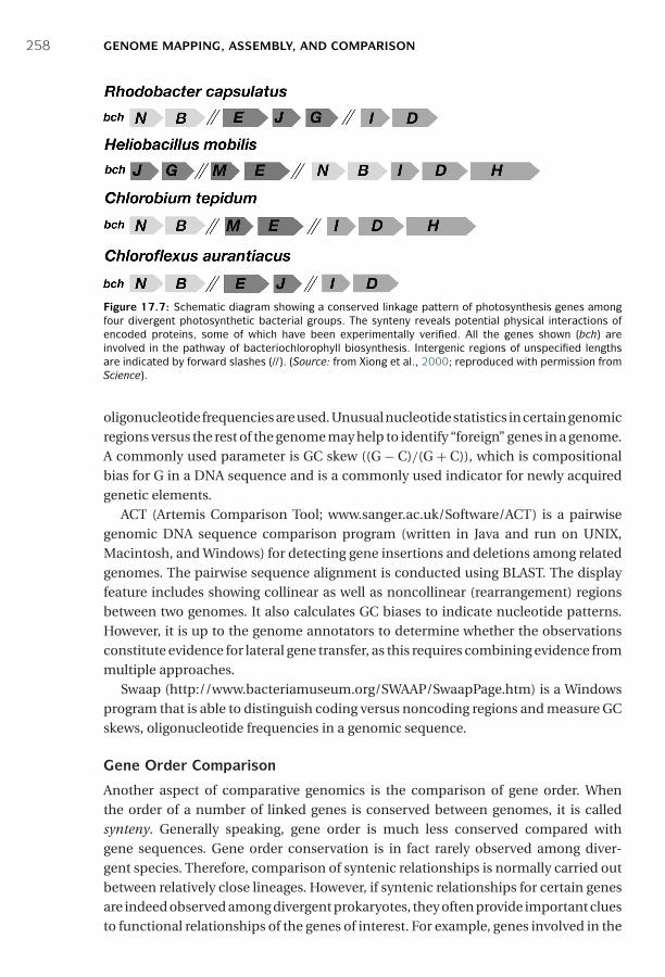
P1: JZP0521840988c17 CB1022/Xiong 0 521 84098 8 January 10, 2006 11:58
258 GENOME MAPPING, ASSEMBLY, AND COMPARISON
Figure 17.7: Schematic diagram showing a conserved linkage pattern of photosynthesis genes amongfour divergent photosynthetic bacterial groups. The synteny reveals potential physical interactions ofencoded proteins, some of which have been experimentally verified. All the genes shown (bch) areinvolved in the pathway of bacteriochlorophyll biosynthesis. Intergenic regions of unspecified lengthsare indicated by forward slashes (//). (Source: from Xiong et al., 2000; reproduced with permission fromScience).
oligonucleotide frequencies are used. Unusual nucleotide statistics in certain genomicregions versus the rest of the genome may help to identify “foreign” genes in a genome.A commonly used parameter is GC skew ((G − C)/(G + C)), which is compositionalbias for G in a DNA sequence and is a commonly used indicator for newly acquiredgenetic elements.
ACT (Artemis Comparison Tool; www.sanger.ac.uk/Software/ACT) is a pairwisegenomic DNA sequence comparison program (written in Java and run on UNIX,Macintosh, and Windows) for detecting gene insertions and deletions among relatedgenomes. The pairwise sequence alignment is conducted using BLAST. The displayfeature includes showing collinear as well as noncollinear (rearrangement) regionsbetween two genomes. It also calculates GC biases to indicate nucleotide patterns.However, it is up to the genome annotators to determine whether the observationsconstitute evidence for lateral gene transfer, as this requires combining evidence frommultiple approaches.
Swaap (http://www.bacteriamuseum.org/SWAAP/SwaapPage.htm) is a Windowsprogram that is able to distinguish coding versus noncoding regions and measure GCskews, oligonucleotide frequencies in a genomic sequence.
Gene Order Comparison
Another aspect of comparative genomics is the comparison of gene order. Whenthe order of a number of linked genes is conserved between genomes, it is calledsynteny. Generally speaking, gene order is much less conserved compared withgene sequences. Gene order conservation is in fact rarely observed among diver-gent species. Therefore, comparison of syntenic relationships is normally carried outbetween relatively close lineages. However, if syntenic relationships for certain genesare indeed observed among divergent prokaryotes, they often provide important cluesto functional relationships of the genes of interest. For example, genes involved in the
P1: JZP0521840988c17 CB1022/Xiong 0 521 84098 8 January 10, 2006 11:58
FURTHER READING 259
same metabolic pathway tend to be clustered among phylogenetically diverse organ-isms. The preservation of the gene order is a result of the selective pressure to allow thegenes to be coregulated and function as an operon. Furthermore, the synteny of genesfrom divergent groups often associates with physical interactions of the encoded geneproducts. The use of conserved gene neighbors as predictors of protein interactionsis discussed in Chapter 18. An example of synteny of bacterial photosynthesis genescoupled with protein interactions is illustrated in Figure 17.7.
GeneOrder (http://pumpkins.ib3.gmu.edu:8080/geneorder/) is a web-based pro-gram that allows direct comparison of a pair of genomic sequences of less than 2 Mb.It displays a dot plot with diagonal lines denoting collinearity of genes and lines offthe diagonal indicating inversions or rearrangements in the genomes.
SUMMARY
Genome mapping using relative positions of genetic markers without knowledgeof sequence data is a low-resolution approach to describing genome structures. Agenome can be described at the highest resolution by a complete genome sequence.Whole-genome sequencing can be carried out using full shotgun or hierarchicalapproaches. The former requires more extensive computational power in the assem-bly step, and the latter is inefficient because of the physical mapping process required.Among the genome sequence assembly programs, ARACHNE and EULER are the bestperformers. Genome annotation includes gene finding and assignment of function tothese genes. Functional assignment depends on homology searching and literatureinformation. GO projects aim to facilitate automated annotation by standardizingthe descriptions used for gene functions. The exact number of genes in the humangenome is unknown, but is likely to be in the same range as most other eukaryotes.The gene number, however, does not dictate complexities of a genome. One exampleis exhibited in protein expression in which a larger number of proteins are producedthan genes available to code for them. This is the so-called genome economy. The mainmechanisms responsible for genome economy are alternative splicing and exon shuf-fling. Genomes can be compared on the basis of their gene content and gene order.Many specialized genome comparison programs for cross-genome alignment havebeen developed. Among them, BLASTZ and LAGAN may be the best in terms of speedand accuracy. Gene order comparison across genomes often helps to discover poten-tial operons and assign putative functions. Conserved gene order among prokaryotesis often indicative of protein physical interactions.
FURTHER READING
Bennetzen, J. 2002. Opening the door to comparative plant biology. Science 296:60–3.Chain, P., Kurtz, S., Ohlebusch, E., and Slezak, T. 2003. An applications-focused review of com-
parative genomics tools: Capabilities, limitations and future challenges. Brief. Bioinform.4:105–23.
P1: JZP0521840988c17 CB1022/Xiong 0 521 84098 8 January 10, 2006 11:58
260 GENOME MAPPING, ASSEMBLY, AND COMPARISON
Dandekar, T, Snel, B., Huynen, M., and Bork, P. 1998. Conservation of gene order: A fingerprintof proteins that physically interact. Trends Biochem. Sci. 23:324–8.
Frazer, K. A., Elnitski, L., Church, D. M., Dubchak, I., and Hardison, R. C. 2003. Cross-speciessequence comparisons: A review of methods and available resources. Genome Res. 13:1–12.
Gibson, G., and Muse, S. V. 2002. A Primer of Genome Science. Sunderland, MA: SinauerAssociates.
Karlin, S., Mrazek, J., and Gentles, A. J. 2003. Genome comparisons and analysis. Curr. Opin.Struct. Biol. 13:344–52.
Lewis, R., and Palevitz, B. A. 2001. Genome economy. The Scientist 15:21.Lio, P. 2003. Statistical bioinformatic methods in microbial genome analysis. BioEssays
25:266–73.Michalovich, D., Overington, J., and Fagan, R. 2002. Protein sequence analysis in silico: Appli-
cation of structure-based bioinformatics to genomic initiatives. Curr. Opin. Pharmacol.2:574–80.
Pennacchio, L. A., and Rubin, E. M. 2003. Comparative genomic tools and databases: Providinginsights into the human genome. J. Clin. Invest. 111:1099–106.
Primrose, S. B., and Twyman, R. M. 2003. Principles of Genome Analysis and Genomics, 3rd ed.Oxford, UK: Blackwell.
Stein, L. 2001. Genome annotation: From sequence to biology. Nat. Rev. Genetics 2:493–503.Sterky, F., and Lundeberg, J. 2000. Sequence analysis of gene and genomes. J. Biotechnol. 76:1–31.Ureta-Vidal, A., Ettwiller, L., and Birney, E. 2003. Comparative genomics: Genome-wide analysis
of metazoan eukaryotes. Nature Rev. Genetics 4:251–62.Waterston, R. H., Lindblad-Toh, K., Birney, E., Rogers, J., Abril, J. F., Agarwal, P., Agarwala,
R., et al. 2002. Initial sequencing and comparative analysis of the mouse genome. Nature420:520–62.
Wei, L., Liu, Y., Dubchak, I., Shon, J., and Park, J. 2002. Comparative genomics approaches tostudy organism similarities and differences. J. Biomed. Inform. 35:142–50.
Xiong, J., Fischer, W. M., Inoue, K., Nakahara, M., and Bauer, C. E. 2000. Molecular evidence forthe early evolution of photosynthesis. Science 289:1724–30.
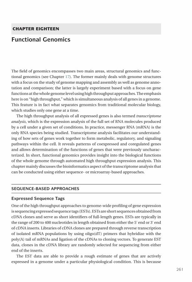
P1: JzG0521840988c18 CB1022/Xiong 0 521 84098 8 January 10, 2006 12:10
CHAPTER EIGHTEEN
Functional Genomics
The field of genomics encompasses two main areas, structural genomics and func-tional genomics (see Chapter 17). The former mainly deals with genome structureswith a focus on the study of genome mapping and assembly as well as genome anno-tation and comparison; the latter is largely experiment based with a focus on genefunctions at the whole genome level using high throughput approaches. The emphasishere is on “high throughput,” which is simultaneous analysis of all genes in a genome.This feature is in fact what separates genomics from traditional molecular biology,which studies only one gene at a time.
The high throughput analysis of all expressed genes is also termed transcriptomeanalysis, which is the expression analysis of the full set of RNA molecules producedby a cell under a given set of conditions. In practice, messenger RNA (mRNA) is theonly RNA species being studied. Transcriptome analysis facilitates our understand-ing of how sets of genes work together to form metabolic, regulatory, and signalingpathways within the cell. It reveals patterns of coexpressed and coregulated genesand allows determination of the functions of genes that were previously uncharac-terized. In short, functional genomics provides insight into the biological functionsof the whole genome through automated high throughput expression analysis. Thischapter mainly discusses the bioinformatics aspect of the transcriptome analysis thatcan be conducted using either sequence- or microarray-based approaches.
SEQUENCE-BASED APPROACHES
Expressed Sequence Tags
One of the high throughput approaches to genome-wide profiling of gene expressionis sequencing expressed sequence tags (ESTs). ESTs are short sequences obtained fromcDNA clones and serve as short identifiers of full-length genes. ESTs are typically inthe range of 200 to 400 nucleotides in length obtained from either the 5′ end or 3′ endof cDNA inserts. Libraries of cDNA clones are prepared through reverse transcriptionof isolated mRNA populations by using oligo(dT) primers that hybridize with thepoly(A) tail of mRNAs and ligation of the cDNAs to cloning vectors. To generate ESTdata, clones in the cDNA library are randomly selected for sequencing from eitherend of the inserts.
The EST data are able to provide a rough estimate of genes that are activelyexpressed in a genome under a particular physiological condition. This is because
261

P1: JzG0521840988c18 CB1022/Xiong 0 521 84098 8 January 10, 2006 12:10
262 FUNCTIONAL GENOMICS
the frequencies for particular ESTs reflect the abundance of the corresponding mRNAin a cell, which corresponds to the levels of gene expression at that condition. Anotherpotential benefit of EST sampling is that, by randomly sequencing cDNA clones, it ispossible to discover new genes.
However, there are also many drawbacks of using ESTs for expression profile anal-ysis. EST sequences are often of low quality because they are automatically generatedwithout verification and thus contain high error rates. Many bases are ambiguouslydetermined, represented by N ’s. Common errors also include frameshift errors andartifactual stop codons, resulting in failures of translating the sequences. In addition,there is often contamination by vector sequence, introns (from unspliced RNAs), ribo-somal RNA (rRNA), mitochondrial RNA, among others. ESTs represent only partialsequences of genes. Gene sequences at the 3′ end tend to be more heavily repre-sented than those at the 5′ end because reverse transcription is primed with oligo(dT)primers. Unfortunately, the sequences from the 3′ end are also most error pronebecause of the low base-call quality at the start of sequence reads. Another prob-lem of ESTs is the presence of chimeric clones owing to cloning artifacts in libraryconstruction, in which more than one transcript is ligated in a clone resulting inthe 5′ end of a sequence representing one gene and the 3′ end another gene. It hasbeen estimated that up to 11% of cDNA clones may be chimeric. Another fundamen-tal problem with EST profiling is that it predominantly represents highly expressed,abundant transcripts. Weakly expressed genes are hardly found in a EST sequencingsurvey.
Despite these limitations, EST technology is still widely used. This is because ESTlibraries can be easily generated from various cell lines, tissues, organs, and at vari-ous developmental stages. ESTs can also facilitate the unique identification of a genefrom a cDNA library; a short tag can lead to a cDNA clone. Although individual ESTsare prone to error, an entire collection of ESTs contains valuable information. Often,after consolidation of multiple EST sequences, a full-length cDNA can be derived.By searching a nonredundant EST collection, one can identify potential genes ofinterest.
The rapid accumulation of EST sequences has prompted the establishment ofpublic and private databases to archive the data. For example, GenBank has a specialEST database, dbEST (www.ncbi.nlm.nih.gov/dbEST/) that contains EST collectionsfor a large number of organisms (>250). The database is regularly updated to reflectthe progress of various EST sequencing projects. Each newly submitted EST sequenceis subject to a database search. If a strong similarity to a known gene is found, it isannotated accordingly.
EST Index Construction
One of the goals of the EST databases is to organize and consolidate the largelyredundant EST data to improve the quality of the sequence information so thedata can be used to extract full-length cDNAs. The process includes a preprocessingstep that removes vector contaminants and masks repeats. Vecscreen, introduced in

P1: JzG0521840988c18 CB1022/Xiong 0 521 84098 8 January 10, 2006 12:10
SEQUENCE-BASED APPROACHES 263
Chapter 17, can be used to screen out bacterial vector sequences. This is followedby a clustering step that associates EST sequences with unique genes. The next stepis to derive consensus sequences by fusing redundant, overlapping ESTs and to cor-rect errors, especially frameshift errors. This step results in longer EST contigs. Theprocedure is somewhat similar to the genome assembly of shotgun sequence reads(see Chapter 17) . Finally, the coding regions are defined through the use of HMM-based gene-finding algorithms (see Chapter 8). This helps to exclude the potentialintron and 3′-untranslated sequences. Once the coding sequence is identified, it canbe annotated by translating it into protein sequences for database similarity search-ing. To go another step further, compiled ESTs can be used to align with the genomicsequence if available to identify the genome locus of the expressed gene as well asintron–exon boundaries of the gene. This is usually performed using the programSIM4 (http://pbil.univ-lyon1.fr/sim4.php).
The clustering process that reduces the EST redundancy and produces a collectionof nonredundant and annotated EST sequences is known as gene index construction.The following lists a couple of major databases that index EST sequences.
UniGene (www.ncbi.nlm.nih.gov/UniGene/) is an NCBI EST cluster database.Each cluster is a set of overlapping EST sequences that are computationally processedto represent a single expressed gene. The database is constructed based on com-bined information from dbEST, GenBank mRNA database, and “electronically spliced”genomic DNA. Only ESTs with 3′ poly-A ends are clustered to minimize the the prob-lem of chimerism. The resulting 3′ EST sequences provide more unique representa-tion of the transcripts. The next step is to remove contaminant sequences that includebacterial vectors and linker sequences. The cleaned ESTs are used to search against adatabase of known unique genes (EGAD database) with the BLAST program. The com-piling step identifies sequence overlaps and derives sequence consensus using theCAP3 program. During this step, errors in individual ESTs are corrected; the sequencesare then partitioned into clusters and assembled into contigs. The final result isa set of nonredundant, gene-oriented clusters known as UniGene clusters. EachUniGene cluster represents a unique gene and is further annotated for putative func-tion and its gene locus information, as well as information related to the tissue typewhere the gene has been expressed. The entire clustering procedure is outlined inFigure 18.1.
TIGR Gene Indices (www.tigr.org/tdb/tgi.shtml) is an EST database that uses adifferent clustering method from UniGene (Fig. 18.2). It compiles data from dbEST,GenBank mRNA and genomic DNA data, and TIGR’s own sequence database.Sequences are only clustered if they are more than 95% identical for over a forty-nucleotide region in pairwise comparisons. BLAST and FASTA are used to identifysequence overlaps. In the sequence assembly stage, both TIGR Assembler (see Chap-ter 17) and CAP3 are used to construct contigs, producing a so-called tentative consen-sus (TC). To prevent chimerism, transcripts are clustered only if they match fully withknown genes. Functional assignment is then given to the TC that relies most heav-ily on BLAST searches against protein databases. The TIGR gene indices serve as an
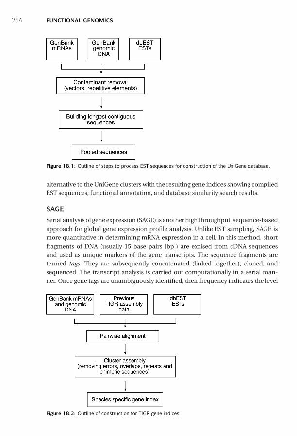
P1: JzG0521840988c18 CB1022/Xiong 0 521 84098 8 January 10, 2006 12:10
264 FUNCTIONAL GENOMICS
Figure 18.1: Outline of steps to process EST sequences for construction of the UniGene database.
alternative to the UniGene clusters with the resulting gene indices showing compiledEST sequences, functional annotation, and database similarity search results.
SAGE
Serial analysis of gene expression (SAGE) is another high throughput, sequence-basedapproach for global gene expression profile analysis. Unlike EST sampling, SAGE ismore quantitative in determining mRNA expression in a cell. In this method, shortfragments of DNA (usually 15 base pairs [bp]) are excised from cDNA sequencesand used as unique markers of the gene transcripts. The sequence fragments aretermed tags. They are subsequently concatenated (linked together), cloned, andsequenced. The transcript analysis is carried out computationally in a serial man-ner. Once gene tags are unambiguously identified, their frequency indicates the level
Figure 18.2: Outline of construction for TIGR gene indices.
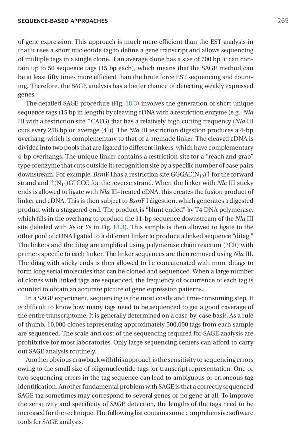
P1: JzG0521840988c18 CB1022/Xiong 0 521 84098 8 January 10, 2006 12:10
SEQUENCE-BASED APPROACHES 265
of gene expression. This approach is much more efficient than the EST analysis inthat it uses a short nucleotide tag to define a gene transcript and allows sequencingof multiple tags in a single clone. If an average clone has a size of 700 bp, it can con-tain up to 50 sequence tags (15 bp each), which means that the SAGE method canbe at least fifty times more efficient than the brute force EST sequencing and count-ing. Therefore, the SAGE analysis has a better chance of detecting weakly expressedgenes.
The detailed SAGE procedure (Fig. 18.3) involves the generation of short uniquesequence tags (15 bp in length) by cleaving cDNA with a restriction enzyme (e.g., NlaIII with a restriction site ↑CATG) that has a relatively high cutting frequency (Nla IIIcuts every 256 bp on average (44)). The Nla III restriction digestion produces a 4-bpoverhang, which is complementary to that of a premade linker. The cleaved cDNA isdivided into two pools that are ligated to different linkers, which have complementary4-bp overhangs. The unique linker contains a restriction site for a “reach and grab”type of enzyme that cuts outside its recognition site by a specific number of base pairsdownstream. For example, BsmF I has a restriction site GGGAC(N10)↑ for the forwardstrand and ↑(N14)GTCCC for the reverse strand. When the linker with Nla III stickyends is allowed to ligate with Nla III–treated cDNA, this creates the fusion product oflinker and cDNA. This is then subject to BsmF I digestion, which generates a digestedproduct with a staggered end. The product is “blunt ended” by T4 DNA polymerase,which fills in the overhang to produce the 11-bp sequence downstream of the Nla IIIsite (labeled with Xs or Ys in Fig. 18.3). This sample is then allowed to ligate to theother pool of cDNA ligated to a different linker to produce a linked sequence “ditag.”The linkers and the ditag are amplified using polymerase chain reaction (PCR) withprimers specific to each linker. The linker sequences are then removed using Nla III.The ditag with sticky ends is then allowed to be concatenated with more ditags toform long serial molecules that can be cloned and sequenced. When a large numberof clones with linked tags are sequenced, the frequency of occurrence of each tag iscounted to obtain an accurate picture of gene expression patterns.
In a SAGE experiment, sequencing is the most costly and time-consuming step. Itis difficult to know how many tags need to be sequenced to get a good coverage ofthe entire transcriptome. It is generally determined on a case-by-case basis. As a ruleof thumb, 10,000 clones representing approximately 500,000 tags from each sampleare sequenced. The scale and cost of the sequencing required for SAGE analysis areprohibitive for most laboratories. Only large sequencing centers can afford to carryout SAGE analysis routinely.
Another obvious drawback with this approach is the sensitivity to sequencing errorsowing to the small size of oligonucleotide tags for transcript representation. One ortwo sequencing errors in the tag sequence can lead to ambiguous or erroneous tagidentification. Another fundamental problem with SAGE is that a correctly sequencedSAGE tag sometimes may correspond to several genes or no gene at all. To improvethe sensitivity and specificity of SAGE detection, the lengths of the tags need to beincreased for the technique. The following list contains some comprehensive softwaretools for SAGE analysis.
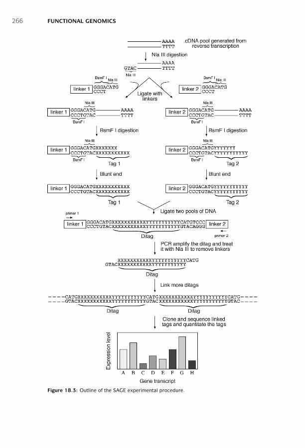
P1: JzG0521840988c18 CB1022/Xiong 0 521 84098 8 January 10, 2006 12:10
266 FUNCTIONAL GENOMICS
Figure 18.3: Outline of the SAGE experimental procedure.
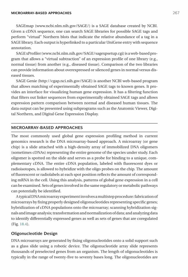
P1: JzG0521840988c18 CB1022/Xiong 0 521 84098 8 January 10, 2006 12:10
MICROARRAY-BASED APPROACHES 267
SAGEmap (www.ncbi.nlm.nih.gov/SAGE/) is a SAGE database created by NCBI.Given a cDNA sequence, one can search SAGE libraries for possible SAGE tags andperform “virtual” Northern blots that indicate the relative abundance of a tag in aSAGE library. Each output is hyperlinked to a particular UniGene entry with sequenceannotation.
SAGE xProfiler (www.ncbi.nlm.nih.gov/SAGE/sagexpsetup.cgi) is a web-based pro-gram that allows a “virtual subtraction” of an expression profile of one library (e.g.,normal tissue) from another (e.g., diseased tissue). Comparison of the two librariescan provide information about overexpressed or silenced genes in normal versus dis-eased tissues.
SAGE Genie (http://cgap.nci.nih.gov/SAGE) is another NCBI web-based programthat allows matching of experimentally obtained SAGE tags to known genes. It pro-vides an interface for visualizing human gene expression. It has a filtering functionthat filters out linker sequences from experimentally obtained SAGE tags and allowsexpression pattern comparison between normal and diseased human tissues. Thedata output can be presented using subprograms such as the Anatomic Viewer, Digi-tal Northern, and Digital Gene Expression Display.
MICROARRAY-BASED APPROACHES
The most commonly used global gene expression profiling method in currentgenomics research is the DNA microarray-based approach. A microarray (or genechip) is a slide attached with a high-density array of immobilized DNA oligomers(sometimes cDNAs) representing the entire genome of the species under study. Eacholigomer is spotted on the slide and serves as a probe for binding to a unique, com-plementary cDNA. The entire cDNA population, labeled with fluorescent dyes orradioisotopes, is allowed to hybridize with the oligo probes on the chip. The amountof fluorescent or radiolabels at each spot position reflects the amount of correspond-ing mRNA in the cell. Using this analysis, patterns of global gene expression in a cellcan be examined. Sets of genes involved in the same regulatory or metabolic pathwayscan potentially be identified.
A typical DNA microarray experiment involves a multistep procedure: fabrication ofmicroarrays by fixing properly designed oligonucleotides representing specific genes;hybridization of cDNA populations onto the microarray; scanning hybridization sig-nals and image analysis; transformation and normalization of data; and analyzing datato identify differentially expressed genes as well as sets of genes that are coregulated(Fig. 18.4).
Oligonucleotide Design
DNA microarrays are generated by fixing oligonucleotides onto a solid support suchas a glass slide using a robotic device. The oligonucleotide array slide representsthousands of preselected genes from an organism. The length of oligonucleotides istypically in the range of twenty-five to seventy bases long. The oligonucleotides are
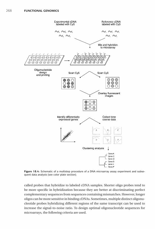
P1: JzG0521840988c18 CB1022/Xiong 0 521 84098 8 January 10, 2006 12:10
268 FUNCTIONAL GENOMICS
Figure 18.4: Schematic of a multistep procedure of a DNA microarray assay experiment and subse-quent data analysis (see color plate section).
called probes that hybridize to labeled cDNA samples. Shorter oligo probes tend tobe more specific in hybridization because they are better at discriminating perfectcomplementary sequences from sequences containing mismatches. However, longeroligos can be more sensitive in binding cDNAs. Sometimes, multiple distinct oligonu-cleotide probes hybridizing different regions of the same transcript can be used toincrease the signal-to-noise ratio. To design optimal oligonucleotide sequences formicroarrays, the following criteria are used.
P1: JzG0521840988c18 CB1022/Xiong 0 521 84098 8 January 10, 2006 12:10
MICROARRAY-BASED APPROACHES 269
The probes should be specific enough to minimize cross-hybridization with non-specific genes. This requires BLAST searches against genome databases to findsequence regions with least sequence similarity with nontarget genes. The probesshould be sensitive and devoid of low-complexity regions (a string of identicalnucleotides; see Chapter 4). The filtering program RepeatMasker (see Chapter 4) isoften used in the BLAST search. The oligonucleotide sequences should not form stableinternal secondary structures, such as a hairpin structure, which could interfere withthe hybridization reaction. DNA/RNA folding programs such as Mfold can help todetect secondary structures. The oligo design should be close to the 3′ end of the genebecause the cDNA collection is often biased to the 3′ end. In addition, for operationalconvenience, all the probes should have an approximately equal melting temperature(Tm) and a GC content of 45% to 65%. A number of programs have been developedthat use these rules in designing probe sequences for microarrays spotting.
OligoWiz (www.cbs.dtu.dk/services/OligoWiz/) is a Java program that runs locallybut allows the user to connect to the server to perform analysis via a graphic user inter-face. It designs oligonucleotides by incorporating multiple criteria including homol-ogy, Tm, low complexity, and relative position within a transcript.
OligoArray (http://berry.engin.umich.edu/oligoarray2/) is also a Java client-serverprogram that computes oligonucleotides for microarray construction. It uses thenormal criteria with an emphasis on gene specificity and secondary structure foroligonucleotides. The secondary structures and related thermodynamic parametersare calculated using Mfold.
Data Collection
The expression of genes is measured via the signals from cDNAs hybridizing with thespecific oligonucleotide probes on the microarray. The cDNAs are obtained by extract-ing total RNA or mRNA from tissues or cells and incorporating fluorescent dyes in theDNA strands during the cDNA biosynthesis. The most common type of microarrayprotocol is the two-color microarray, which involves labeling one set of cDNA froman experimental condition with one dye (Cy5, red fluorescence) and another set ofcDNA from a reference condition (the controls) with another dye (Cy3, green fluores-cence). When the two differently labeled cDNA samples are mixed in equal quantityand allowed to hybridize with the DNA probes on the chips, gene expression patternsof both samples can be measured simultaneously.
The image of the hybridized array is captured using a laser scanner that scansevery spot on the microarray. Two wavelengths of the laser beam are used to excitethe red and green fluorescent dyes to produce red and green fluorescence, which isdetected using a photomultiplier tube. Thus, for each spot on the microarray, redand green fluorescence signals are recorded. The two fluorescence images from thescanner are then overlaid to create a composite image, which indicates the relativeexpression levels of each gene. Thus, the measurement from the composite imagereflects the ratio of the two color intensities. If a gene is expressed at a higher levelin the experimental condition (red) than in the control (green), the spot displays
P1: JzG0521840988c18 CB1022/Xiong 0 521 84098 8 January 10, 2006 12:10
270 FUNCTIONAL GENOMICS
a reddish color. If the gene is expressed at a lower level than the control, the spotappears greenish. Unchanged gene expression, having equal amount of green andred fluorescence, results in a yellow spot. The colored image is stored as a computerfile (in TIFF format) for further processing.
Image Processing
Image processing is to locate and quantitate hybridization spots and to separate truehybridization signals from background noise. The background noise and artifacts pro-duced in this step include nonspecific hybridization, unevenness of the slide surface,and the presence of contaminants such as dust on the surface of the slide. In addi-tion, there are also geometric variations of hybridization spots resulting in some spotsbeing of irregular shapes. Computer programs are used to correctly locate the bound-aries of the spots and measure the intensities of the spot images after subtracting thebackground pixels.
After subtracting the background noise, the array signals are converted into num-bers and reported as ratios between Cy5 and Cy3 for each spot. This ratio representsrelative expression changes and reflects the fold change in mRNA quantity in experi-mental versus control conditions. The data are often presented as false colors of dif-ferent intensities of red and green colors depending on whether the ratios are above 1or below 1, respectively. Where there is an equal quantity of experimental and controlmRNA (yellow in raw data), black is shown. The false color images are presented insquares in a matrix of genes versus conditions so that differentially expressed genescan be more easily analyzed (Box 18.1).
Manufacturers of microarray scanners normally provide software programs tospecifically perform microarray image analysis. There are, however, also a small num-ber of free image-processing software programs available on the Internet.
ArrayDB (http://genome.nhgri.nih.gov/arraydb/) is a web interface program thatallows the user to upload data for graphical viewing. The user can present histograms,select actual microarray slide images, and display detailed information of each spotwhich is linked to functional annotation of the corresponding gene in the UniGene,Entrez, dbEST, and KEGG databases. This can help to provide a synopsis of genefunction when interpreting the microarray data.
ScanAlyze (http://rana.lbl.gov/EisenSoftware.htm) is a Windows program formicroarray fluorescent image analysis. It features semiautomatic spot definition andmultichannel pixel and spot analyses.
TIGR Spotfinder (http://www.tigr.org/softlab/) is another Windows program formicroarray image processing using the TIFF image format. It uses an adaptive thresh-old algorithm, which resolves the boundaries of spots according to their shapes. Thealgorithm determines the intensity of irregular spots more accurately than most othersimilar programs. It also interfaces with a gene expression database.
Data Transformation and Normalization
Following image processing, the digitized gene expression data need to be furtherprocessed before differentially expressed genes can be identified. This processing is

P1: JzG0521840988c18 CB1022/Xiong 0 521 84098 8 January 10, 2006 12:10
MICROARRAY-BASED APPROACHES 271
Box 18.1 Outline of the Procedure for Microarray Data Analysis
The example involves the use of six hypothetic genes whose expression is measuredover a time course of 5 hours. The microarray raw data in the form of Cy5/Cy3 ratiosare converted to false colors image in red, green and black. The data matrix is sub-jected to logarithmic transformation. The distances between genes are calculatedusing Pearson correlation coefficients. After conversion to a positive distancematrix, further classification analysis using the hierarchical clustering approachproduces a tree showing the relationships of coexpressed genes (see color platesection).
referred to as data normalization and is designed to correct bias owing to variationsin microarray data collection rather than intrinsic biological differences.
When the raw fluorescence intensity Cy5 is plotted against Cy3, most of the data areclustered near the bottom left of the plot, showing a non-normal distribution of theraw data (Fig. 18.5A). This is thought to be a result of the imbalance of red and greenintensities during spot sampling, resulting in ineffective discrimination of differen-tially expressed genes. One way to improve the data discrimination is to transform
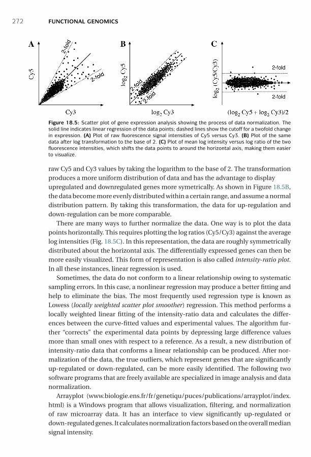
P1: JzG0521840988c18 CB1022/Xiong 0 521 84098 8 January 10, 2006 12:10
272 FUNCTIONAL GENOMICS
Figure 18.5: Scatter plot of gene expression analysis showing the process of data normalization. Thesolid line indicates linear regression of the data points; dashed lines show the cutoff for a twofold changein expression. (A) Plot of raw fluorescence signal intensities of Cy5 versus Cy3. (B) Plot of the samedata after log transformation to the base of 2. (C) Plot of mean log intensity versus log ratio of the twofluorescence intensities, which shifts the data points to around the horizontal axis, making them easierto visualize.
raw Cy5 and Cy3 values by taking the logarithm to the base of 2. The transformationproduces a more uniform distribution of data and has the advantage to displayupregulated and downregulated genes more symetrically. As shown in Figure 18.5B,the data become more evenly distributed within a certain range, and assume a normaldistribution pattern. By taking this transformation, the data for up-regulation anddown-regulation can be more comparable.
There are many ways to further normalize the data. One way is to plot the datapoints horizontally. This requires plotting the log ratios (Cy5/Cy3) against the averagelog intensities (Fig. 18.5C). In this representation, the data are roughly symmetricallydistributed about the horizontal axis. The differentially expressed genes can then bemore easily visualized. This form of representation is also called intensity-ratio plot.In all these instances, linear regression is used.
Sometimes, the data do not conform to a linear relationship owing to systematicsampling errors. In this case, a nonlinear regression may produce a better fitting andhelp to eliminate the bias. The most frequently used regression type is known asLowess (locally weighted scatter plot smoother) regression. This method performs alocally weighted linear fitting of the intensity-ratio data and calculates the differ-ences between the curve-fitted values and experimental values. The algorithm fur-ther “corrects” the experimental data points by depressing large difference valuesmore than small ones with respect to a reference. As a result, a new distribution ofintensity-ratio data that conforms a linear relationship can be produced. After nor-malization of the data, the true outliers, which represent genes that are significantlyup-regulated or down-regulated, can be more easily identified. The following twosoftware programs that are freely available are specialized in image analysis and datanormalization.
Arrayplot (www.biologie.ens.fr/fr/genetiqu/puces/publications/arrayplot/index.html) is a Windows program that allows visualization, filtering, and normalizationof raw microarray data. It has an interface to view significantly up-regulated ordown-regulated genes. It calculates normalization factors based on the overall mediansignal intensity.
P1: JzG0521840988c18 CB1022/Xiong 0 521 84098 8 January 10, 2006 12:10
MICROARRAY-BASED APPROACHES 273
SNOMAD (http://pevsnerlab.kennedykrieger.org/snomadinput.html) is a webserver for microarray data normalization. It provides scatter plots based on raw signalintensities and performs log-transformation and linear regression as well as Lowessregression analysis of the data.
Statistical Analysis to Identify Differentially Expressed Genes
To separate genes that are differentially expressed, many published studies use a nor-malization cutoff of twofold as a criterion. However, this is an arbitrary cutoff value,which could be considered to be either too high or too low depending on the datavariability. In addition, the inherent data variability is not taken into account. A datapoint above or below the cutoff line could simply be there by chance or because oferror. The only way to ensure that a gene that appears to be differentially expressedis truly differentially expressed is to perform multiple replicate experiments and toperform statistical testing. The repeat experiments provide replicate data points thatoffer information about the variability of the expression data at a particular condition.The information on the distribution for the data points under particular conditionscan help answer the question whether a given fold difference is significant. The mainhindrance to obtaining multiple replicate datasets is often the cost: microarray exper-iments are extremely expensive for regular research laboratories.
If replicated datasets are available, rigorous statistical tests such as t-test and anal-ysis of variance (ANOVA) can be performed to test the null hypothesis that a givendata point is not significantly different from the mean of the data distribution. Forsuch tests, it is common to use a P-value cutoff of .05, which means a confidence levelof 95% to distinguish the data groups. This level also corresponds to a gene expres-sion level with two standard deviations from the mean of distribution. It is noticeablethat the number of standard deviations is only meaningful if the data are approx-imately normally distributed, which makes the previous normalization step morevaluable.
MA-ANOVA (www.jax.org/staff/churchill/labsite/software/anova/) is a statisticalprogram for Windows and UNIX that uses ANOVA to analyze microarray data. It cal-culates log ratios, displays ratio-intensity plots, and performs permutation tests andbootstrapping of confidence values.
Cyber-T (http://visitor.ics.uci.edu/genex/cybert/) is a web server that performst-tests on observed changes of replicate gene expression measurements to identifysignificantly differentially expressed genes. It also contains a computational methodfor estimating false-positive and false-negative levels in experimental data based onmodeling of P-value distributions.
Microarray Data Classification
One of the key features of DNA microarray analysis is to study the expression of manygenes in parallel and identify groups of genes that exhibit similar expression patterns.The similar expression patterns are often a result of the fact that the genes involved

P1: JzG0521840988c18 CB1022/Xiong 0 521 84098 8 January 10, 2006 12:10
274 FUNCTIONAL GENOMICS
are in the same metabolic pathway and have similar functions. The genetic basis ofthe coregulation could be the result of common promoters and regulatory regions.
To discover genes with similar gene expression patterns based on the microarraydata requires partitioning the data into subsets according to similarity. To achieve thisgoal, hybridization signals from microarray images are organized into matrices whererows represent genes and columns represent experimental sampling conditions (suchas time points or drug concentrations). Each matrix value is the Cy5/Cy3 intensity ratiorepresenting the relative expression of a gene under a specific condition (see Box 18.1).Various classification tools are subsequently used to classify the values in the matricesfor gene expression comparison.
Distance MeasureThe first step towards gene classification is to define a measure of the distance ordissimilarity between genes. This requires converting a gene expression matrix ina distance matrix. The distance can be expressed as Euclidean distance or Pearsoncorrelation coefficient. Euclidean distance is the square root of the sum of squareddistances between expression data points. When comparing X gene expression with Ygene expression at time point i (assuming there are n time points in total), the distancescore (d) can be calculated by the following formula:
d =√√√√ n∑
i=1
(xi − y i)2 (Eq. 18.1)
Euclidean distances are widely used but suffer from the problem that when variationsbetween genes are very small, the gene profiles can be very difficult to differentiate.
Alternatively, a Pearson correlation coefficient between two groups of data pointscan be used. This measures the overall similarity between the trends or shapes of thetwo sets of data. In this measure, a perfect positive correlation is +1 and a perfectnegative correlation is −1. The distance score (d ) between gene X and gene Y can becalculated using the following formula:
d = 1n
n∑i=1
(xi − x
sdi
) (yi − yi
sdi
)(Eq. 18.2)
where n is the total number of time points; x and y are average values for the X geneand Y gene data, respectively; and sd are standard deviation values.
The choice of the distance measures can sometimes make a big difference in thefinal result. Sometimes, a small change in expression data can cause a significantchange in an Euclidean distance matrix. Pearson correlation coefficients are morerobust than Euclidean distances in guarding against small variations and noise inthe experimental data. One notable feature of the Pearson correlation coefficientsis that, when the genes to be compared have exactly the same expression patterns,their gene expression profiles have identical shapes. The correlation coefficient of thegene profiles equals to +1, in which case, the relative distance between the genes
P1: JzG0521840988c18 CB1022/Xiong 0 521 84098 8 January 10, 2006 12:10
MICROARRAY-BASED APPROACHES 275
is zero. When the concerned genes have absolute opposite expression patterns, thecorrelation coefficient becomes −1. That means that, when one gene is up-regulated,the other is down-regulated, and vice versa. In such case, the distance is converted to+2 (the absolute value of |(−1) − 1|), the maximum distance value in the matrix (seeBox 18.1). The conversion to a positive distance value makes data classification moreconvenient.
Supervised and Unsupervised ClassificationBased on the computed distances between genes in an expression profile, genes withsimilar expression patterns can be grouped. The classification analysis can be eithersupervised or unsupervised. A supervised analysis refers to classification of data intoa set of predefined categories. For example, depending on the purpose of the exper-iment, the data can be classified into predefined “diseased” or “normal” categories.An unsupervised analysis does not assume predefined categories, but identifies datacategories according to actual similarity patterns. The unsupervised analysis is alsocalled clustering, which is to group patterns into clusters of genes with correlatedprofiles.
For microarray data, clustering analysis identifies coexpressed and coregulatedgenes. Genes within a category have more similarity in expression than genes fromdifferent categories. When genes are coregulated, they normally reflect related func-tionality. Through gene clustering, functions of previously uncharacterized genes maybe discovered. Clustering methods include hierarchical clustering and partitioningclustering (e.g., k-means, self-organizing maps [SOMs]). The following discussionfocuses on several of the most frequently used clustering methods.
The clustering algorithms can be further divided into two types, agglomerative anddivisive (Fig. 18.6). An agglomerative method begins by clustering the two most similardata points and repeats the process to successively merge groups of data accordingto similarity until all groups of data are merged. This is also known as the bottom-upapproach. A divisive method works the other way around by lumping all data pointsin a single cluster and successively dividing the data into smaller groups accordingto dissimilarity until all the hierarchical levels are resolved. This is also called thetop-down approach.
Hierarchical Clustering. A hierarchical clustering method is in principle similar to thedistance phylogenetic tree-building method (see Chapter 11). It produces a treelikestructure that represents a hierarchy or relative relatedness of data groups. In the treeleaves, similar gene expression profiles are placed more closely together than dissim-ilar gene expression profiles. The tree-branching pattern illustrates a higher degree ofrelationship between related gene groups. When genes with similar expression pro-files are grouped in such a way, functions for unknown genes can often be inferred.
Hierarchical clustering uses the agglomerative approach that works in much thesame way as the UPGMA method (see Chapter 11), in which the most similar datapairs are joined first to form a cluster. The new cluster is treated as a single entity

P1: JzG0521840988c18 CB1022/Xiong 0 521 84098 8 January 10, 2006 12:10
276 FUNCTIONAL GENOMICS
Figure 18.6: Schematic representation showing differences between agglomerative and divisive clus-tering methods.
creating a reduced matrix. The reduced matrix allows the next closest data point to beadded to the previous cluster leading to the formation of a new cluster. By repeatingthe process, a dendrogram showing the clustering pattern of all data points is built.
The hierarchical clustering algorithms can be further divided in three subtypesknown as single linkage, complete linkage, and average linkage. The single linkagemethod chooses the minimum value of a pair of distances as the cluster distance.The complete linkage method chooses the maximum value of a pair of distances, andthe average linkage method chooses the mean of the two distances, which is the sameas the UPGMA tree building approach. The UPGMA-based method is considered tobe the most robust in discriminating expression clusters. It is important to point outthat although a tree structure is produced as the final result, the resulting tree has noevolutionary meaning, but merely represents groupings of similarity patterns in geneexpression.
In a tree produced by hierarchical clustering, the user has the flexibility to define athreshold for determining the boundaries of data clusters. The flexibility, however,sometimes can be a disadvantage in that it lacks objective criteria to distinguishclusters. Another potential drawback is that the hierarchical relationships of geneexpression represented by the tree may not in fact exist. Some of the drawbacks canbe alleviated by using alternative clustering approaches such as the k-means or self-organizing maps.
k-Means Clustering. In contrast to hierarchical clustering algorithms, k-means clus-tering does not produce a dendrogram, but instead classifies data through a singlestep partition. Thus, it is a divisive approach. In this method, data are partitioned intok-clusters, which are prespecified at the outset. The value of k is normally randomlyset but can be adjusted if results are found to be unsatisfactory. In the first step, data
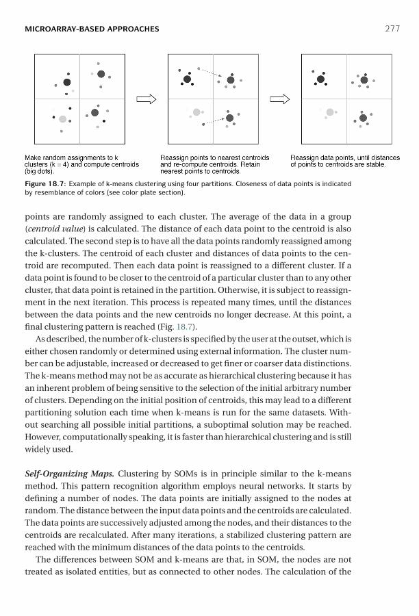
P1: JzG0521840988c18 CB1022/Xiong 0 521 84098 8 January 10, 2006 12:10
MICROARRAY-BASED APPROACHES 277
Figure 18.7: Example of k-means clustering using four partitions. Closeness of data points is indicatedby resemblance of colors (see color plate section).
points are randomly assigned to each cluster. The average of the data in a group(centroid value) is calculated. The distance of each data point to the centroid is alsocalculated. The second step is to have all the data points randomly reassigned amongthe k-clusters. The centroid of each cluster and distances of data points to the cen-troid are recomputed. Then each data point is reassigned to a different cluster. If adata point is found to be closer to the centroid of a particular cluster than to any othercluster, that data point is retained in the partition. Otherwise, it is subject to reassign-ment in the next iteration. This process is repeated many times, until the distancesbetween the data points and the new centroids no longer decrease. At this point, afinal clustering pattern is reached (Fig. 18.7).
As described, the number of k-clusters is specified by the user at the outset, which iseither chosen randomly or determined using external information. The cluster num-ber can be adjustable, increased or decreased to get finer or coarser data distinctions.The k-means method may not be as accurate as hierarchical clustering because it hasan inherent problem of being sensitive to the selection of the initial arbitrary numberof clusters. Depending on the initial position of centroids, this may lead to a differentpartitioning solution each time when k-means is run for the same datasets. With-out searching all possible initial partitions, a suboptimal solution may be reached.However, computationally speaking, it is faster than hierarchical clustering and is stillwidely used.
Self-Organizing Maps. Clustering by SOMs is in principle similar to the k-meansmethod. This pattern recognition algorithm employs neural networks. It starts bydefining a number of nodes. The data points are initially assigned to the nodes atrandom. The distance between the input data points and the centroids are calculated.The data points are successively adjusted among the nodes, and their distances to thecentroids are recalculated. After many iterations, a stabilized clustering pattern arereached with the minimum distances of the data points to the centroids.
The differences between SOM and k-means are that, in SOM, the nodes are nottreated as isolated entities, but as connected to other nodes. The calculation of the
P1: JzG0521840988c18 CB1022/Xiong 0 521 84098 8 January 10, 2006 12:10
278 FUNCTIONAL GENOMICS
centroid values in SOM takes into account not only information from within eachcluster, but also information from adjacent clusters. This allows the analysis to bebetter at handling noisy data. Another difference is that, in SOM, some nodes areallowed to contain no data at all. Thus, at the completion of the clustering, the finalnumber of clusters may be smaller than the initial nodes. This feature renders SOMless subjective than k-means. However, this type of algorithm is also much slower thanthe k-means method.
Clustering Programs. Cluster (http://rana.lbl.gov/EisenSoftware.htm) is a Windowsprogram capable of hierarchical clustering, SOM, and k-means clustering. Outputsfrom hierarchical clustering are visualized with the Treeview program.
EPCLUST (www.ebi.ac.uk/EP/EPCLIST) is a web-based server that allows data to beuploaded and clustered with hierarchical clustering or k-means methods. In addition,the user can perform data selection, normalization, and database similarity searcheswith this program.
TIGR TM4 (www.tigr.org/tm4) is a suite of multiplatform programs for analyzingmicroarray data. This comprehensive package includes four interlinked programs,TIGR spot finder (for image analysis), MIDAS (for data normalization), MeV (for clus-tering analysis and visualization), and MADAM (for data management). The packageprovides different data normalization schemes and clustering options.
SOTA (Self-Organizing Tree Algorithm; www.almabioinfo.com/sota/) is a webserver that uses a hybrid approach of SOM and hierarchical clustering. It builds atree based on the divisive approach starting from the root node containing all datapatterns. Instead of using the distance-based criteria to resolve a tree, the algorithmusing the neural network based SOM algorithm to separate clusters of genes at eachnode. The homogeneity of gene clusters at each node is analyzed using SOM. The treebuilding stops at any point if desired homogeneity level is reached.
COMPARISON OF SAGE AND DNA MICROARRAYS
SAGE and DNA microarrays are both high throughput techniques that determineglobal mRNA expression levels. A number of comparative studies have indicatedthat the gene expression measurements from these methods are largely consistentwith each other. However, the two techniques have important differences. First, SAGEdoes not require prior knowledge of the transcript sequence, whereas DNA micro-array experiments can only detect the genes spotted on the microarray. Because SAGEis able to measure all the mRNA expressed in a sample, it has the potential to allowdiscovery of new, yet unknown gene transcripts. Second, SAGE measures “absolute”mRNA expression levels without arbitrary reference standards, whereas DNA microar-rays indicate the relative expression levels. Therefore, SAGE expression data are morecomparable across experimental conditions and platforms. This makes public SAGEdatabases more informative by allowing comparison of data from reference conditionswith various experimental treatments. Third, the PCR amplification step involved in
P1: JzG0521840988c18 CB1022/Xiong 0 521 84098 8 January 10, 2006 12:10
SUMMARY 279
the SAGE procedure means that it requires only a minute quantity of sample mRNA.This compares favorably to the requirement for a much larger quantity of mRNAfor microarray experiments, which may be impossible to obtain under certain cir-cumstances. Fourth, collecting a SAGE library is very labor intensive and expensivecompared with carrying out a DNA microarray experiment, however. Therefore, SAGEis not suitable for rapid screening of cells whereas the microarray analysis is. Fifth,Gene identification from SAGE data is also more cumbersome because the mRNAtags have to be extracted, compiled, and identified computationally, whereas in DNAmicroarrays, the identities of the probes are already known. In SAGE, comparison ofgene expression profiles to discover differentially expressed genes and coexpressedgenes is performed manually, whereas for microarrays, there are a large number ofsoftware algorithms to automate the process.
SUMMARY
Transcriptome analysis using ESTs, SAGE, and DNA microarrays forms the core offunctional genomics and is key to understanding the interactions of genes and theirregulation at the whole-genome level. EST sampling, although widely used, has anumber of drawbacks in terms of error rates, efficiency, and cost. The high through-put SAGE and DNA microarray approaches provide a more quantitative measureof global gene expression. SAGE measures the “absolute” mRNA expression levels,whereas microarrays indicate relative mRNA expression levels. DNA microarrays cur-rently enjoy greater popularity because of the relative ease of experimentation. It is alsoa more suitable method to probe differential gene expression between different tissueand cell samples. This requires comparing gene profiles using statistical approaches.Another goal of microarray analysis is to identify coordinated gene expression pat-terns, which requires clustering analysis of microarray data.
The most popular microarray data clustering techniques include hierarchical clus-tering, SOM, and k-means. The hierarchical approach is very similar to the phylo-genetic distance tree building method. SOM and k-means normally do not generatea treelike structure as a result of clustering. Once coregulated genes are identified,upstream sequences belonging to a cluster can be retrieved and analyzed for com-mon regulatory sequences.
In conclusion, among the three techniques for studying global gene expression, themost popular one is DNA microarrays, which has the capability to provide informationthat is not possible with traditional techniques. However, one should also be aware ofits limitations. This technique is a multistep procedure in which errors and biases canbe introduced in each step (scanning, image processing, normalization, and choice ofclassification method). Thus, it is a rather crude assay and may contain considerablelevels of false positives and false negatives. The results from microarray analysis onlyprovide hypotheses for gene functions based on classification of expression data.To verify the hypotheses, one has to rely on traditional biochemical and molecularbiological approaches. The fundamental limitation of this method lies in the use of
P1: JzG0521840988c18 CB1022/Xiong 0 521 84098 8 January 10, 2006 12:10
280 FUNCTIONAL GENOMICS
transcription as the sole indicator of gene expression, which may or may not correlatewith expression at the protein level. The expression of proteins is what dictates thephenotypes. The last limitation is addressed in Chapter 19.
FURTHER READING
Causton, H. C., Quackenbush, J., and Brazma, A. 2003. Microarray Gene Expression Data Analysis:A Beginner’s Guide. Malden, MA: Blackwell.
Forster, T., Roy, D., and Ghazal, P. 2003. Experiments using microarray technology: Limitationsand standard operating procedure. J. Endocrinol. 178:195–204.
Gill, R. W., and Sanseau, P. 2000. Rapid in silico cloning of genes using expressed sequence tags(ESTs). Biotechnol. Annu. Rev. 5:25–44.
Quackenbush, J. 2002. Microarray data normalization and transformation. Nat Genet. 32(Suppl):496–501.
Scott, H. S., and Chrast, R. 2001. Global transcript expression profiling by Serial Analysis of GeneExpression (SAGE). Genet. Eng. 23:201–19.
Slonim, D. K. 2002. From patterns to pathways: Gene expression data analysis comes of age.Nat. Genet. 32(Suppl):502–8.
Stanton, L. W. 2001. Methods to profile gene expression. Trends Cardiovasc. Med. 11:49–54.Stekel, D. 2003. Microarray Bioinformatics. Cambridge, UK: Cambridge University Press.Ye, S. Q., Usher, D. C., and Zhang, L. Q. 2002. Gene expression profiling of human diseases by
serial analysis of gene expression. J. Biomed. Sci. 9:384–94.
P1: PIG0521840988c19 CB1022/Xiong 0 521 84098 8 January 10, 2006 12:18
CHAPTER NINETEEN
Proteomics
Proteome refers to the entire set of expressed proteins in a cell. In other words, it is thefull complement of translated product of a genome. Proteomics is simply the studyof the proteome. More specifically, it involves simultaneous analyses of all trans-lated proteins in a cell. It encompasses a range of activities including large-scaleidentification and quantification of proteins and determination of their localization,modifications, interactions, and functions. This chapter covers the major topics inproteomics such as analysis of protein expression, posttranslational modifications,protein sorting, and protein–protein interaction with an emphasis on bioinformaticsapplications.
Compared to transcriptional profiling in functional genomics, proteomics has clearadvantages in elucidating gene functions. It provides a more direct approach to under-standing cellular functions because most of the gene functions are realized by proteins.Transcriptome analysis alone does not provide clear answers to cellular functionsbecause there is generally not a one-to-one correlation between messenger RNAs(mRNAs) and proteins in the cells. In addition, a gene in an eukaryotic genome mayproduce more varied translational products owing to alternative splicing, RNA edit-ing, and so on. This means that multiple and distinct proteins may be produced fromone single gene. Further complexities of protein functions can be found in posttrans-lational modifications, protein targeting, and protein–protein interactions. Therefore,the noncorrelation of mRNA with proteins means that studying protein expressioncan provide more insight on understanding of gene functions.
TECHNOLOGY OF PROTEIN EXPRESSION ANALYSIS
Characterization of protein expression at the whole proteome level involves quanti-tative measurement of proteins in a cell at a particular metabolic state. Unlike in DNAmicroarray analysis, in which the identities of the probes are known beforehand, theidentities of the expressed proteins in a proteome have to determined by perform-ing protein separation, identification, quantification, and identification procedures.The classic protein separation methods involve two-dimensional gel electrophoresisfollowed by gel image analysis. Further characterization involves determination ofamino acid composition, peptide mass fingerprints, and sequences using mass spec-trometry (MS). Finally, database searching is needed for protein identification. Theoutline of the procedure is shown in Figure 19.1.
281
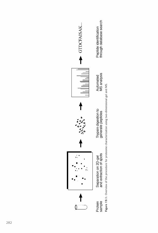
P1: PIG0521840988c19 CB1022/Xiong 0 521 84098 8 January 10, 2006 12:18
Figu
re1
9.1
:O
verv
iew
ofth
epro
cedur
efo
rpro
teom
ech
arac
teri
zation
usin
gtw
o-dim
ensi
onal
gela
ndM
S.
282
P1: PIG0521840988c19 CB1022/Xiong 0 521 84098 8 January 10, 2006 12:18
TECHNOLOGY OF PROTEIN EXPRESSION ANALYSIS 283
2D-Page
Two-dimensional polyacrylamide gel electrophoresis (2D-PAGE) is a high-resolutiontechnique that separates proteins by charge and mass. The gel is run in one directionin a pH gradient under a nondenaturing condition to separate proteins by isoelectricpoints (pI) and then in an orthogonal dimension under a denaturing condition to sep-arate proteins by molecular weights (MW). This is followed by staining, usually silverstaining, which is very sensitive, to reveal the position of all proteins. The result is atwo-dimensional gel map; each spot on the map corresponds to a single protein beingexpressed. The stained gel can be further scanned and digitized for image analysis.
However, not all proteins can be separated by this method or stained properly. Oneof the challenges of this technique is the separation of membrane proteins, whichare largely hydrophobic and not readily solublized. They tend to aggregate in theaqueous medium of a two-dimensional gel. To overcome this problem, membraneproteins can be fractionated using specialized protocols and then electrophoresedusing optimized buffers containing zwitterionic detergents. Subfractionation can becarried out to separate nuclear, cytosol, cytoskeletal, and other subcellular fractionsto boost the concentrations of rare proteins and to reveal subcellular localizations ofthe proteins.
Gel image analysis is the next step that helps to reveal differential global proteinexpression patterns. This analysis includes spot determination, quantitation, and nor-malization. Image analysis software is used to measure the center, edges, and densitiesof the spots. Comparing two-dimensional gel images from various experiments cansometimes pose a challenge because the gels, unlike DNA microarrays, may shrink orwarp. This requires the software programs to be able to stretch or maneuver one ofthe gels relative to the other to find a common geometry. When the reference spots arealigned properly, the rest of the spots can be subsequently compared automatically.There are a number of web-based tools available for this type of image analysis.
Melanie (http://us.expasy.org/melanie/) is a commercially available comprehen-sive software package for Windows. It carries out background subtraction, spot detec-tion, quantitation, annotation, image manipulation and merging, and linking to2D-PAGE databases as well as image comparison through statistical tests.
CAROL (http://gelmatching.inf.fu-berlin.de/Carol.html) is a free Java program fortwo-dimensional gel matching, which takes into account geometrical distortions ofgel spots.
Comp2Dgel (www2.imtech.res.in/raghava/comp2dgel/) is a web server that allowsthe user to compare two-dimensional gel images with a two-dimensional gel databaseor with other gels that the user inputs. A percentage deviation of the images is obtainedthrough superimposition of the images.
SWISS-2DPAGE (www.expasy.ch/) is a database of two-dimensional gel maps ofcells of many organisms at metabolic resting conditions (control conditions), whichcan be used for comparison with experimental or diseased conditions. It can besearched by a spot identifier or keyword.
P1: PIG0521840988c19 CB1022/Xiong 0 521 84098 8 January 10, 2006 12:18
284 PROTEOMICS
Mass Spectrometry Protein Identification
Once the proteins are separated on a two-dimensional gel, they can be further identi-fied and characterized using MS. In this procedure, the proteins from a two-dimensional gel system are first digested in situ with a protease (e.g., trypsin). Proteinspots of interest are excised from the two-dimensional gel. The proteolysis generates aunique pattern of peptide fragments of various MWs, which is termed a peptide finger-print. The fragments can be analyzed with MS, a high-resolution technique for deter-mining molecular masses. Currently, electrospray ionization MS and matrix-assistedlaser desorption ionization (MALDI) MS are commonly used. These two approachesonly differ in the ionization procedure used. In MALDI-MS, for example, the peptidesare charged with positive ions and forced through an analyzing tube with a magneticfield. Peptides are analyzed in the gas phase. Because smaller peptides are deflectedmore than larger ones in a magnetic field, the peptide fragments can be separatedaccording to molecular mass and charges. A detector generates a spectrum that dis-plays ion intensity as a function of the mass-to-charge ratio.
As a step toward further identification, the peptides can be sequenced with suc-cessive phases of fragmentation and mass analysis. This is the technique of tandemmass spectrometry (MS/MS), in which a peptide has to pass through two analyzers forsequence determination. In the first analyzer, the peptide is fragmented by physicalmeans generating fragments with nested sizes differing by only one amino acid. Themolecular masses of these fragments are more precisely determined in the secondanalyzer yielding the sequence of the fragment.
Protein Identification through Database Searching
MS characterization of proteins is highly dependent on bioinformatic analysis. Oncethe peptide mass fingerprints or peptide sequences are determined, bioinformaticsprograms can be used to search for the identity of a protein in a database of the-oretically digested proteins. The purpose of the database search is to find exact ornearly exact matches. However, in reality, protease digestion is rarely perfect, oftengenerating partially digested products as a result of missed cuts at expected cuttingsites. Peptides resulting from MALDI-MS are also charged, which increases their massslightly. To increase the discriminatory ability of the database search, the search enginemust allow some leeway in matching molecular masses of peptides in the cases ofmissed cuts and charge modifications. The user is required to provide as much infor-mation as possible as input. For example, molecular masses of peptide fingerprints,peptide sequence, MW, and pI of the intact protein, even the species names are impor-tant in obtaining unique identification of a particular protein. A basic requirement forpeptide identification through database matching is the availability of all the proteinsequences from an organism. Thus, this method only works well with model organ-isms that have completely sequenced and well-annotated genomes, but has muchlimitation to be applied in nonmodel organisms.
P1: PIG0521840988c19 CB1022/Xiong 0 521 84098 8 January 10, 2006 12:18
TECHNOLOGY OF PROTEIN EXPRESSION ANALYSIS 285
ExPASY (www.expasy.ch/tools/) is a comprehensive proteomics web server witha suite of programs for searching peptide information from the SWISS-PROT andTrEMBL databases. There are twelve database search tools in this server dedicatedto protein identification based on MS data. For example, the AACompIdent programidentifies proteins based on pI, MW, and amino acid composition and comparesthese values with theoretical compositions of all proteins in SWISS-PROT/TrEMBL.The number of candidate proteins can be further narrowed down by using speciesnames and keywords. The TagIdent program can narrow down the candidate list bypeptide sequences because of the high specificity of short sequence matches. ThePeptIdent program incorporates mass fingerprinting information with informationsuch as pI, MW, and species name. Candidate proteins are ranked by the number ofmatching peptides. The CombSearch tool takes advantage of the strength of multipleparameters by using combined composition, sequence tags, and peptide fingerprint-ing information to perform combined searches against the databases.
ProFound (http://prowl.rockefeller.edu/profound bin/WebProFound.exe) is aweb server with a set of interconnected programs. It searches a protein sequencedatabase using MS fingerprinting information. A Bayesian algorithm ranks thedatabase matches according to the probability of database sequences producing thepeptide mass fingerprints.
Mascot (www.matrixscience.com/search form select.html) is another web serverthat identifies proteins based on peptide mass fingerprints, sequence entries, or rawMS/MS data from one or more peptides.
Differential In-Gel Electrophoresis
Differences in protein expression patterns can be detected in a similar way as influorescent-labeled DNA microarrays, using a technique called differential in-gelelectrophoresis (DIGE) (Fig. 19.2). Proteins from experimental and control samplesare labeled with differently colored fluorescent dyes. They are mixed together beforeelectrophoresis on a two-dimensional gel. Differentially expressed proteins in bothconditions can be coseparated and visualized in the same gel. Compared to regular2D-PAGE, the process reduces the noise and improves the reproducibility and sensi-tivity of detection. In principle, it resembles the two-color DNA microarray analysis.The drawbacks of this approach are that different proteins take up fluorescent tags todifferent extents and that some proteins labeled with the fluorophores may becomeless soluble and precipitate before electrophoresis.
Protein Microarrays
Protein microarray chips are conceptually similar to DNA microarray chips (see chap-ter 17) and can be built to contain high-density grids with immobilized proteins forhigh throughput analysis. The chips contain entire immobilized proteome. However,they are not meant to be used to bind and quantitate complementary moleculesas in DNA microarrays. Instead, they are used for studying protein function by
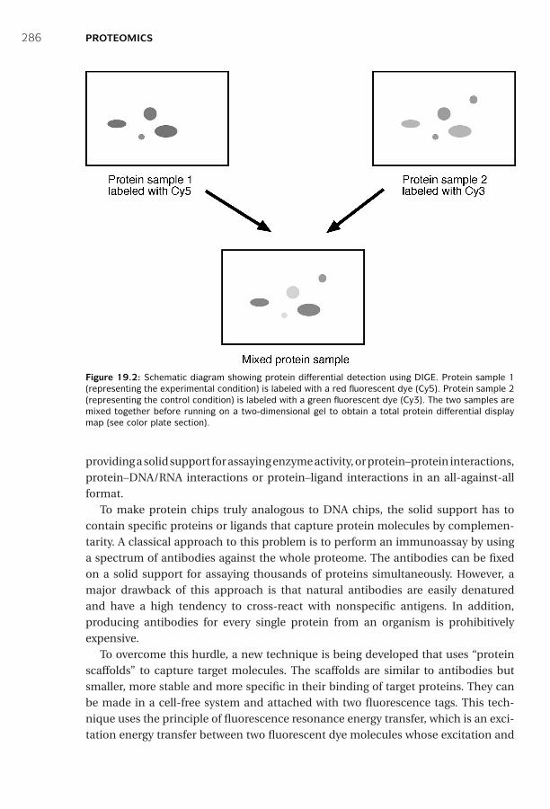
P1: PIG0521840988c19 CB1022/Xiong 0 521 84098 8 January 10, 2006 12:18
286 PROTEOMICS
Figure 19.2: Schematic diagram showing protein differential detection using DIGE. Protein sample 1(representing the experimental condition) is labeled with a red fluorescent dye (Cy5). Protein sample 2(representing the control condition) is labeled with a green fluorescent dye (Cy3). The two samples aremixed together before running on a two-dimensional gel to obtain a total protein differential displaymap (see color plate section).
providing a solid support for assaying enzyme activity, or protein–protein interactions,protein–DNA/RNA interactions or protein–ligand interactions in an all-against-allformat.
To make protein chips truly analogous to DNA chips, the solid support has tocontain specific proteins or ligands that capture protein molecules by complemen-tarity. A classical approach to this problem is to perform an immunoassay by usinga spectrum of antibodies against the whole proteome. The antibodies can be fixedon a solid support for assaying thousands of proteins simultaneously. However, amajor drawback of this approach is that natural antibodies are easily denaturedand have a high tendency to cross-react with nonspecific antigens. In addition,producing antibodies for every single protein from an organism is prohibitivelyexpensive.
To overcome this hurdle, a new technique is being developed that uses “proteinscaffolds” to capture target molecules. The scaffolds are similar to antibodies butsmaller, more stable and more specific in their binding of target proteins. They canbe made in a cell-free system and attached with two fluorescence tags. This tech-nique uses the principle of fluorescence resonance energy transfer, which is an exci-tation energy transfer between two fluorescent dye molecules whose excitation and
P1: PIG0521840988c19 CB1022/Xiong 0 521 84098 8 January 10, 2006 12:18
POSTTRANSLATIONAL MODIFICATIONS 287
absorption spectra overlap. The efficiency of the energy transfer depends on the dis-tance of the two dyes. If one portion of the tagged protein is involved in binding toa target protein, the protein conformational changes cause the two fluorescent tagsto move apart, disrupting the excitation energy transfer between the dyes such that itcan be monitored on fluorescence spectra.
A technology called Protein-Print is in early development, which is essentially amolecular imprinting method. Chemical monomers are used to coat target proteins,which are then allow to polymerize. When polymerization is complete and the targetmolecules removed, a mould is formed that resembles the shape of the target protein.The moulds can then be used to capture like molecules with high specificity.
These are some of the promising technologies currently under development. Theirhigh throughput nature means that they may eventually succeed the two-dimensionalgel-based method. When the proteome chips become available, data analysis foridentifying coregulated proteins should be relatively easy because it will be similar tothat used for DNA microarrays. Similar image analysis and clustering algorithms canbe applied to identify coregulated proteins.
POSTTRANSLATIONAL MODIFICATIONS
Another important aspect of the proteome analysis concerns posttranslational mod-ifications. To assume biological activity, many nascent polypeptides have to be cova-lently modified before or after the folding process. This is especially true in eukary-otic cells where most modifications take place in the endoplasmic reticulum andthe Golgi apparatus. The modifications include proteolytic cleavage; formation ofdisulfide bonds; addition of phosphoryl, methyl, acetyl, or other groups onto certainamino acid residues; or attachment of oligosaccharides or prosthetic groups to createmature proteins. Posttranslational modifications have a great impact on protein func-tion by altering the size, hydrophobicity and overall conformation of the proteins. Themodifications can directly influence protein–protein interactions and distribution ofproteins to different subcellular locations.
It is therefore important to use bioinformatics tools to predict sites for posttransla-tional modifications based on specific protein sequences. However, prediction of suchmodifications can often be difficult because the short lengths of the sequence motifsassociated with certain modifications. This often leads to many false-positive identifi-cations. One such example is the known consensus motif for protein phosphorylation,[ST]-x-[RK]. Such a short motif can be found multiple times in almost every proteinsequence. Most of the predictions based on this sequence motif alone are likely to bewrong, producing very high rates of false-positives. Similar situations can be found inother predicted modification sites. One of the reasons for the false predictions is thatneighboring environment of the modification sites is not considered.
To minimize false-positive results, a statistical learning process called supportvector machine (SVM) can be used to increase the specificity of prediction. This is

P1: PIG0521840988c19 CB1022/Xiong 0 521 84098 8 January 10, 2006 12:18
288 PROTEOMICS
a data classification method similar to the linear or quadratic discriminant analysis(see Chapter 8). In this method, the data are projected in a three-dimensional spaceor even a multidimensional space. A hyperplane – a linear or nonlinear mathematicalfunction – is used to best separate true signals from noise. The algorithm has moreenvironmental variables included that may be required for the enzyme modification.After training the algorithm with sufficient structural features, it is able to correctlyrecognize many posttranslational modification patterns.
AutoMotif (http://automotif.bioinfo.pl/) is a web server predicting proteinsequence motifs using the SVM approach. In this process, the query sequence is chop-ped up into a number of overlapping fragments, which are fed into different kernels(similar to nodes). A hyperplane, which has been trained to recognize known pro-tein sequence motifs, separates the kernels into different classes. Each separation iscompared with known motif classes, most of which are related to posttranslationalmodification. The best match with a known class defines the functional motif.
Prediction of Disulfide Bridges
A disulfide bridge is a unique type of posttranslational modification in which cova-lent bonds are formed between cysteine residues. Disulfide bonds are important formaintaining the stability of certain types of proteins.
The disulfide prediction is the prediction of paring potential or bonding states ofcysteines in a protein. Accurate prediction of disulfide bonds may also help to predictthe three-dimensional structure of the protein of interest. This problem can be tack-led by using either profiles constructed from multiple sequence alignment or residuecontact potentials calculated based on the local sequence environment. Advancedneural networks or SVM or hidden Markov model (HMM) algorithms are often usedto discern long-distance pairwise interactions among cysteine residues. The fol-lowing program is one of the publicly available programs specialized in disulfideprediction.
Cysteine (http://cassandra.dsi.unifi.it/cysteines/) is a web server that predicts thedisulfide bonding states of cysteine residues in a protein sequence by building profilesbased on multiple sequence alignment information. A recursive neural network (seeChapter 14) ranks the candidate residues for disulfide formation.
Identification of Posttranslational Modifications in Proteomic Analysis
Posttranslational modifications can be experimentally identified based on MS fin-gerprinting data. Certain peptide identification tools are able to search for knownposttranslational modification sites in a sequence and incorporate extra mass basedon the type of modifications during database fragment matching. There are two sub-programs in the ExPASY proteomics server and an independent RESID database thatare related to predicting posttranslational modifications.
ExPASY (www.expasy.ch/tools) contains a number of programs to determine post-translational modifications based on MS molecular mass data. FindMod is a sub-program that uses experimentally determined peptide fingerprint information to
P1: PIG0521840988c19 CB1022/Xiong 0 521 84098 8 January 10, 2006 12:18
PROTEIN SORTING 289
compare the masses of the peptide fragments with those of theoretical peptides. If adifference is found, it predicts a particular type of modification based on a set of prede-fined rules. It can predict twenty-eight types of modifications, including methylation,phosphorylation, lipidation, and sulfation. GlyMod is a subprogram that specializes inglycosylation determination based on the difference in mass between experimentallydetermined peptides and theoretical ones.
RESID (http://pir.georgetown.edu/pirwww/search/textresid.html) is an indepen-dent posttranslational modification database listing 283 types of known modifica-tions. It can search by text or MWs.
PROTEIN SORTING
Subcellular localization is an integral part of protein functionality. Many proteinsexhibit functions only after being transported to certain compartments of the cell.The study of the mechanism of protein trafficking and subcellular localization is thefield of protein sorting (also known as protein targeting), which has become one of thecentral themes in modern cell biology. Identifying protein subcellular localization is animportant aspect of functional annotation, because knowing the cellular localizationof a protein often helps to narrow down its putative functions.
For many eukaryotic proteins, newly synthesized protein precursors have to betransported to specific membrane-bound compartments and be proteolytically pro-cessed to become functional. These compartments include chloroplasts, mitochon-dria, the nucleus, and peroxisomes. To carry out protein translocation, unique peptidesignals have to be present in the nascent proteins, which function as “zip codes” thatdirect the proteins to each of these compartments. Once the proteins are translocatedwithin the organelles, protease cleavage takes place to remove the signal sequencesand generate mature proteins (another example of posttranslational modification).Even in prokaryotes, proteins can be targeted to the inner or outer membranes, theperiplasmic space between these membranes, or the extracellular space. The sortingof these proteins is similar to that in eukaryotes and relies on the presence of signalpeptides.
The signal sequences have a weak consensus but contain some specific features.They all have a hydrophobic core region preceded by one or more positively chargedresidues. However, the length and sequence of the signal sequences vary tremen-dously. Peptides targeting mitochondria, for example, are located in the N-terminalregion. The sequences are typically twenty to eighty residues long, rich in positivelycharged residues such as arginines as well as hydroxyl residues such as serines andthreonines, but devoid of negatively charged residues, and have the tendency to formamphiphilic α-helices. These targeting sequences are cleaved once the precursor pro-teins are inside the mitochondria. Chloroplast localization signals (also called transitpeptides) are also located in the N-terminus and are about 25 to 100 residues in length,containing very few negatively charged residues but many hydroxylated residues suchas serine. An interesting feature of the proteins targeted for the chloroplasts is that the
P1: PIG0521840988c19 CB1022/Xiong 0 521 84098 8 January 10, 2006 12:18
290 PROTEOMICS
transit signals are bipartite. That is, they consist of two adjacent signal peptides, onefor targeting the proteins to the stroma portion of the chloroplast before being cleavedand the other for targeting the remaining portion of the proteins to the thylakoids.Localization signals targeting to the nucleus are variable in length (seven to forty-oneresidues) and are found in the internal region of the proteins. They typically consist ofone or two stretches of basic residues with a consensus motif K(K/R)X(K/R). Nuclearsignal sequences are not cleaved after protein transport.
Considerable variations in length and sequence make accurate prediction of signalpeptides using computational approaches difficult. Nonetheless, various computa-tional methods have been developed to predict the subcellular localization signals. Ingeneral, they fall within three categories. Some algorithms are signal based, dependingon the knowledge of charge, hydrophobicity, or consensus motifs. Some are contentbased, depending on the sequence statistics such as amino acid composition. Thethird group of algorithm combines the virtue of both signals and content and appearsto be more successful in prediction. Neural network- and HMM-based algorithms areexamples of the combined approach. Here are some of the most frequently used pro-grams for the prediction of subcellular localization and protein sorting signals withreasonable accuracy (65% to 70%).
SignalP (www.cbs.dtu.dk/services/SignalP-2.0/#submission) is a web-based pro-gram that predicts subcellular localization signals by using both neural networks andHMMs. The neural network algorithm combines two different scores, one for recogniz-ing signal peptides and the other for protease cleavage sites. The HMM-based analysisdiscriminates between signal peptides and the N-terminal transmembrane anchorsegments required for insertion of the protein into the membrane. The program istrained by three different training sets, namely, eukaryotes, Gram-negative bacteriaand Gram-positive bacteria. This distinction is necessary because there are signifi-cant differences in the characteristics of the signal peptides from these organisms.Therefore, appropriate datasets need to be selected before analyzing the sequence.The program predicts both the signal peptides and the protease cleavage sites of thequery sequence.
TargetP (www.cbs.dtu.dk/services/TargetP/) is a neural network-based program,similar to SignalP. It predicts the subcellular locations of eukaryotic proteins basedon their N-terminal amino acid sequence only. It uses analysis output from SignalPand feeds it into a decision neural network, which makes a final choice regarding thetarget compartment.
PSORT (http://psort.nibb.ac.jp/) is a web server that uses a nearest neighbormethod to make predictions of subcellular localizations. It compares the querysequence to a library of signal peptides for different cellular localizations. If themajority of the closest signal peptide matches (nearest neighbors) are for a partic-ular cellular location, the sequence is predicted as signal peptide for that location. It isfunctionally similar to TargetP, but may have lower sensitivity. An iPSORT is availablein the same website that predicts N-terminal sorting signals and is an equivalent toSignalP.

P1: PIG0521840988c19 CB1022/Xiong 0 521 84098 8 January 10, 2006 12:18
PROTEIN–PROTEIN INTERACTIONS 291
PROTEIN–PROTEIN INTERACTIONS
In general, proteins have to interact with each other to carry out biochemical func-tions. Thus, mapping out protein–protein interactions is another important aspect ofproteomics. Interprotein interactions include strong interactions that allow forma-tion of stable complexes and weaker ones that exist transiently. Proteins involved informing complexes are generally more tightly coregulated in expression than thoseinvolved in transient interactions. Protein–protein interaction analysis at the pro-teome level helps reveal the function of previously uncharacterized proteins on thebasis of the “guilt by-association” rule.
Experimental Determination
Protein interactions are commonly detected by using the classic yeast two-hybridmethod that relies on the interaction of “bait” and “prey” proteins in molecular con-structs in yeast. In this strategy, a two-domain transcriptional activator is employedas a helper for determining protein–protein interactions. The two domains whichare a DNA-binding domain and a trans-activation domain normally interact to acti-vate transcription. However, molecular constructs are made such that each of thetwo domains is covalently attached to each of the two candidate proteins (bait andprey). If the bait and prey proteins physically interact, they bring the DNA-binding andtrans-activation domains in such close proximity that they reconstitute the functionof the transcription activator, turning on the expression of a reporter gene as a result.If the two candidate proteins do not interact, the reporter gene expression remainsswitched off.
This technique is essentially a low throughput approach because each bait and preyconstruct has to be prepared individually to map interactions between all proteins.Nonetheless, it has been systematically applied to study interactions at the wholeproteome level. Protein–protein interaction networks of yeast and a small number ofother species have been subsequently determined using this method. A major flaw inthis method is that it is an indirect approach to probe protein–protein interaction andhas a tendency to generate false positives (spurious interactions) and false negatives(undetected interactions). It has been estimated from proteome-wide characteriza-tions that the rate of false positives can be as high as 50%. Another weakness is thatonly pairwise interactions are measured, and therefore interactions that only takeplace when multiple proteins come together are omitted.
There are many alternative approaches to determining protein–protein interac-tions. One of them is to use a large-scale affinity purification technique that involvesattaching fusion tags to proteins and purifying the associated protein complexesin an affinity chromatography column. The purified proteins are then analyzed bygel electrophoresis followed by MS for identification of the interacting components.The protein microarray systems mentioned above also provide a high throughputalternative for studying protein–protein interactions. Although none of the methods

P1: PIG0521840988c19 CB1022/Xiong 0 521 84098 8 January 10, 2006 12:18
292 PROTEOMICS
Figure 19.3: Rosetta stone method for prediction of genes encoding interacting proteins based ondomain fusion patterns in different genomes. In genome A, two different domains exist in separateopen reading frames. In genome B, they are fused together in one protein-encoding frame. Conversely,the two domains of the same protein encoded in genome B may become separate in genome A, but stillperform the same function through physical interactions.
are guaranteed to eliminate false positives and false negatives, combining multipleapproaches in theory compensates for the potential weaknesses of each techniqueand minimizes the artifacts.
Prediction of Protein–Protein Interactions
Decades of research on protein biochemistry and molecular biology has accumulatedtremendous amount of data related to protein–protein interactions, which allow theextraction of some general rules governing these interactions. These rules have facil-itated the development of algorithms for automated prediction of protein–proteininteractions. The currently available tools are generally based on evolutionary stud-ies of gene sequences, gene linkage patterns, and gene fusion patterns, which aredescribed in detail next.
Predicting Interactions Based on Domain FusionOne of the prediction methods is based on gene fusion events. The rationale goes likethis: if A and B exist as interacting domains in a fusion protein in one proteome, thegene encoding the protein is a fusion gene. Their homologous gene sequences A′ andB′ existing separately in another genome most likely encode proteins interacting toperform a common function. Conversely, if ancestral genes A and B encode interactingproteins, they may have a tendency to be fused together in other genomes duringevolution to enhance their effectiveness. This method of predicting protein–proteininteractions is called the “Rosetta stone” method (Fig. 19.3) because a fused proteinoften reveals relationships between its domain components.
The further justification behind this method is that when two domains are fusedin a single protein, they have to be in extremely close proximity to perform a commonfunction. When the two domains are located in two different proteins, to preservethe same functionality, their close proximity and interaction have to be preservedas well. Therefore, by studying gene/protein fusion events, protein–protein interac-tions can be predicted. This prediction rule has been proven to be rather reliable andsince successfully applied to a large number of proteins from both prokaryote andeukaryotes.
P1: PIG0521840988c19 CB1022/Xiong 0 521 84098 8 January 10, 2006 12:18
PROTEIN–PROTEIN INTERACTIONS 293
Predicting Interactions Based on Gene NeighborsGene orders, generally speaking, are poorly conserved among divergent prokaryoticgenomes (see Chapter 16). However, if a certain gene linkage is found to be indeedconserved across divergent genomes, it can be used as a strong indicator of formationof an operon that encodes proteins that are functionally and even physically coupled.This rule of predicting protein–protein interactions holds up for most prokaryoticgenomes. For eukaryotic genomes, gene order may be a less potent predictor of proteininteractions than a tight coregulation for gene expression.
Predicting Interactions Based on Sequence HomologyIf a pair of proteins from one proteome are known to interact, their conservedhomologs in another proteome are likely to have similar interactions. The homolo-gous pairs are referred to as interologs. This method relies on the correct identificationof orthologs and the use of existing protein interaction databases. The method haspotential to model protein quaternary structure if one pair of proteins have knownstructures.
InterPreTS (www.russell.embl-heidelberg.de/people/patrick/interprets/interprets.html) is a web server that has a built-in database for interacting domains basedon known three-dimensional protein structures. Two protein sequences are usedas query to search against the database for homologs. The alignment of the querysequences and database domains is carried out using HMMer (see Chapter 6). Ifthe alignment scores for both sequences are above the threshold and the contactresidues are found to be conserved, the two proteins are considered to be interactingproteins.
IPPRED (http://cbi.labri.fr/outils/ippred/IS part simple.php) is a similar web-based program that allows the user to submit multiple protein sequences. Theprogram searches homologous sequences using BLAST in a database of known inter-acting protein pairs (BIND). If any two query sequences have strong enough simi-larity with known interacting protein pairs, they are inferred as interacting partners.
Predicting Interactions Based on Phylogenetic InformationProtein interactions can be predicted using phylogenetic profiles, which are defined aspatterns of gene pairs that are concurrently present or absent across genomes. In otherwords, this method detects the copresence or co-absence of orthologs across a numberof genomes. Genes having the same pattern of presence or absence across genomesare predicted as encoding interacting proteins. The logic behind the cooccurrenceapproach is that proteins normally operate as a complex. If one of the components ofthe complex is lost, it results in the failure of the entire complex. Under the selectivepressure, the rest of the nonfunctional interacting partners in the complex are alsolost during evolution because they have become functionally unnecessary. The rulebased on concurrent gene loss or gene gain has proven to be less accurate than therules based on gene fusion and gene neighbors. An example of using the phylogeneticprofile method to predict interacting proteins is shown in Figure 19.4.

P1: PIG0521840988c19 CB1022/Xiong 0 521 84098 8 January 10, 2006 12:18
294 PROTEOMICS
Figure 19.4: Phylogenetic profile method for predicting interacting proteins based on copresence andco-absence of the encoding genes across genomes. The presence is indicated by checks and absenceby dashed lines. The protein pairs encoded by genes one and three as well as genes two and four arepredicted as interacting partners.
A more quantitative phylogenetic method to predict protein interactions is the“mirror tree” method, which examines the resemblance between phylogenetic treesof two sequence families (Fig. 19.5). The rationale is that if two protein trees are nearlyidentical in topology and are highly correlated in terms of evolutionary rate, theyare highly likely to interact with each other. This is because if mutations occur at
Figure 19.5: Mirror tree method for prediction of interacting proteins based on strong statistical corre-lation of evolutionary distance matrices used to build two phylogenetic trees for the two protein familiesof interest. The two trees have a near identical topology resulting in a near mirror image. The distancematrices used to construct the trees are compared using correlation analysis.
P1: PIG0521840988c19 CB1022/Xiong 0 521 84098 8 January 10, 2006 12:18
PROTEIN–PROTEIN INTERACTIONS 295
the interaction surface for one of the proteins, corresponding mutations are likelyto occur in the interacting partner to sustain the interaction. As a result, the twointeracting proteins should have very similar phylogenetic trees reflecting very similarevolutionary history. To analyze the extent of coevolution, correlation coefficients (r)of evolutionary distance matrices for the two groups of protein homologs used inconstructing the trees are examined. It has been shown that if r > 0.8, there is a strongindication for protein interactions.
Matrix (http://orion.icmb.utexas.edu/cgi-bin/matrix/matrix-index.pl) is a webserver that predicts interaction between two protein families. The server aligns twoindividual protein data sets (assuming each representing a protein family) usingClustal. It then derives distance matrices from the two alignment files and alignsthe matrices to discover similar portions that may indicate interacting partners fromthe two protein families.
ADVICE (Automated Detection and Validation of Interaction based on the Co-Evolutions, http://advice.i2r.a-star.edu.sg/) is a similar web server providing predic-tion of interacting proteins using the mirror-tree approach. It performs automatedBLAST searches for a given protein sequence pair to derive two sets of homologoussequences. The sequences are multiply aligned using CLUSTAL. A distance matrix foreach set of alignment is then derived. The Pearson’s correlation coefficient is subse-quently calculated for detecting similarities between the two distance matrices. If thecoefficient r > 0.8, the two query sequences are predicted to be a interacting pair.
Predicting Interactions Using Hybrid MethodsIt needs to be emphasized that each of these prediction methods is based on a partic-ular hypothesis and may exhibit a certain degree of bias associated with the hypoth-esis. Because it is difficult to evaluate the performance of each individual predictionmethod, the user of these prediction algorithms is recommended to use a combinedapproach that uses multiple methods to reduce bias and error rates and to yield ahigher level of confidence in the protein interaction prediction. The following inter-net program is a good example of combining multiple lines of evidence in predictingprotein-protein interactions.
STRING (Search Tool for the Retrieval of Interacting Genes/Proteins, http://www.bork.embl-heidelberg.de/STRING/) is a web server that predicts gene and pro-tein functional associations based on combined evidence of gene linkage, genefusion and phylogenetic profiles. The current version also includes experimental co-expression data as well as documented interactions resulted from literature mining.Functional associations include both direct and indirect protein-protein interactions.Indirect interactions can mean enzymes in the same pathway sharing a common sub-strate or proteins regulating each other in the genetic pathway. The server containsinformation for orthologous groups from 110 completely sequenced genomes. Thequery sequence is first classified into an orthologous group based on the COG classi-fication (see Chapter 7) and is then used to search the database for known conservedlinkage pattern, gene fusions, and phylogenetic profiles. The server uses a weighted
P1: PIG0521840988c19 CB1022/Xiong 0 521 84098 8 January 10, 2006 12:18
296 PROTEOMICS
scoring system that evaluates the significance of all three types of protein associationsamong the genomes. To reduce false positives and increase reliability of the prediction,the three types of genomic associations are checked against an internal reference set.A single score of pairwise interactions is given as the final output which also containsall three types of evidence plus a summary of combined protein interaction networkinvolving multiple partners. The server returns a list of predicted protein-proteinassociations and a graphic representation of the association network.
SUMMARY
Protein expression analysis at the proteome level promises more accurate elucida-tion of cellular functions. This is an advantage over genomic analysis, which doesnot necessarily lead to prediction of protein functions. Traditional experimentalapproaches to proteomics include large-scale protein identification using 2D-PAGEand MS. The identification process requires the integration of bioinformatics toolsto search databases for matching peptides. Newer protein expression profiling tech-niques include DIGE and protein microarrays. Protein functions can be modulated asa result of posttranslational modifications. Sequence based prediction often resultsin high rates of false-positives owing to limited understanding of the structural fea-tures required for the modifications. A step toward minimizing the false-positive ratesin prediction is the use of SVM. Another area of proteomics is defining protein sub-cellular localization signals. Several web tools such as TargetP, SignalP, and PSORT areavailable to give reasonably successful prediction of signal peptides. Protein–proteininteractions are normally determined using yeast two-hybrid experiments or otherexperimental methods. However, theoretical prediction of such interactions is pro-viding a promising alternative. The current prediction methods are based on domainfusion, gene linkage pattern, sequence homology, and phylogenetic information. Theability to predict protein interactions is of tremendous value in genome annotationand in understanding the function of genes and their encoded proteins. The compu-tational approach helps to generate hypotheses to be tested by experiments.
FURTHER READING
Aebersold, R., and Mann, M. 2003. Mass spectrometry-based proteomics. Nature 422:198–207.Cutler, P. 2003. Protein arrays: The current state-of-the-art. Proteomics 3:3–18.Donnes, P., and Hoglund, A. 2004. Predicting protein subcellular localization: past, present, and
future. Genomics Proteomics Bioinformatics 2:209–15.Droit, A., Poirier, G. G., and Hunter, J. M. 2005. Experimental and bioinformatic approaches for
interrogating protein-protein interactions to determine protein function. J. Mol. Endocrinol.34:263–80.
Eisenhaber, F., Eisenhaber, B., and Maurer-Stroh, S. 2003. “Prediction of post-translational mod-ifications from amino acid sequence: Problems, pitfalls, and methodological hints.” In Bioin-formatics and Genomes: Current Perspectives, edited by M. A. Andrade, 81–105. Wymondham,UK: Horizon Scientific Press.
Emanuelsson, O. 2002. Predicting protein subcellular localisation from amino acid sequenceinformation. Brief. Bioinform. 3:361–76.

P1: PIG0521840988c19 CB1022/Xiong 0 521 84098 8 January 10, 2006 12:18
FURTHER READING 297
Huynen, M. A., Snel, B., Mering, C., and Bork, P. 2003. Function prediction and protein networks.Curr. Opin. Cell Biol. 15:191–8.
Mann, M., and Jensen, O. N. 2003. Proteomic analysis of post-translational modifications.Nature Biotechnol. 21:255–61.
Nakai, K. 2000. Protein sorting signals and prediction of subcellular localization. Adv. ProteinChem. 54:277–344.
Nakai, K. 2001. Review: Prediction of in vivo fates of proteins in the era of genomics and pro-teomics. J. Struct. Biol. 134:103–16.
Phizicky, E., Bastiaens, P. I. H., Zhu, H., Snyder, M., and Fields, S. 2003. Protein analysis on aproteomic scale. Nature 422:208–15.
Sadygov, R. G., Cociorva, D., and Yates, J. R. III. 2004. Large-scale database searching usingtandem mass spectra: Looking up the answer in the back of the book. Nat. Methods 1:195–202.
Tyers, M., and Mann, M. 2003. From genomics to proteomics. Nature 422:193–7.Valencia, A., and Pazos, F. 2002. Computational methods for the prediction of protein interac-
tions. Curr. Opin. Struct. Biol. 12:368–73.Valencia, A., and Pazos, F. 2003. Prediction of protein-protein interactions from evolutionary
information. Methods Biochem. Anal. 44:411–26.

P1: PIG0521840988c19 CB1022/Xiong 0 521 84098 8 January 10, 2006 12:18
298

P1: JzG0521840988apx1 CB1022/Xiong 0 521 84098 8 January 10, 2006 14:28
Appendix
299

P1: JzG0521840988apx1 CB1022/Xiong 0 521 84098 8 January 10, 2006 14:28
300

P1: JzG0521840988apx1 CB1022/Xiong 0 521 84098 8 January 10, 2006 14:28
APPENDIX ONE
Practical Exercises
Note: all exercises were originally designed for use on a UNIX workstation. However,with slight modifications, they can be used on any other operating systems with Internetaccess.
EXERCISE 1. DATABASE SEARCHES
In this exercise, you will learn how to use several biological databases to retrieveinformation according to certan criteria. After learning the basic search techniques,you will be given a number of problems and asked to provide answers from thedatabases.
1. Use a web browser to retrieve a protein sequence of lambda repressorfrom SWISS-PROT (http://us.expasy.org/sprot/). Choose “Full text search inSwiss-Prot and TrEMBL.” In the following page, Enter “lambda repressor”(space is considered as logical operator AND) as keywords in the querywindow. Select “Search in Swiss-Prot only.” Click on the “submit” button.Note the search result contains hypertext links taking you to references thatare cited or to other related information. Spend a little time studying theannotations.
2. In the same database, search more sequences for “human MAP kinaseinhibitor,” “human catalase,” “synechocystis cytochrome P450,” “coli DNApolymerase,” “HIV CCR5 receptor,” and “Cholera dehydrogenase.” Record yourfindings and study the annotations.
3. Go to the SRS server (http://srs6.ebi.ac.uk/) and find human genes that arelarger than 200 kilobase pairs and also have poly-A signals. Click on the “LibraryPage” button. Select “EMBL” in the “Nucleotide sequence databases” section.Choose the “Extended” query form on the left of the page. In the follow-ing page, Select human (“hum”) at the “Division” section. Enter “200000” inthe “SeqLength >=” field. Enter “polya signal” in the “AllText” field. Press the“Search” button. How many hits do you get?
4. Use your knowledge and creativity to do the following SRS exercises.1) Find protein sequences from Rhizobium submitted by Ausubel be-
tween 1991 and 2001 in the UniProt/Swiss-Prot database (hint: the date
301
P1: JzG0521840988apx1 CB1022/Xiong 0 521 84098 8 January 10, 2006 14:28
302 APPENDIX 1. PRACTICAL EXERCISES
expression can be 1-Jan-1991 and 31-Dec-2001). Study the annotations of thesequences.
2) Find full-length protein sequences of mammalian tyrosine phosphataseexcluding partial or fragment sequences in the UniProt/SwissProt database(hint: the taxonic group of mammals is mammalia). Once you get the queryresult, do a Clustal multiple alignment on the first five sequences from thesearch result.
5. Go to the web page of NCBI Entrez (http://www.ncbi.nlm.nih.gov/) and use theadvanced search options to find protein sequences for human kinase modifiedor added in the last 30 days in GenBank. In the Entrez “Protein” database, enter“human[ORGN] kinase”, and then select “last 30 days” in the “ModificationDate” field of the “Limits” section. Select “Only from” “GenBank” as database.Finally, select “ Go.”
6. Using Entrez, search DNA sequences for mouse fas antigen with annotatedexons or introns. (Do not forget to deselect “Limits” from the above exercise.)In Entrez, select the Nucleotide database. Type mouse[ORGN] AND fas AND(exons OR introns). Click “Go.”
7. For the following exercises involving the NCBI databases, design searchstrategies to find answers (you will need to decide which database to usefirst).
1) Find gene sequences for formate dehydrogenase from Methanobac-terium.
2) Find gene sequences for DNA binding proteins in Methanobacterium.3) Find all human nucleotide sequences with D-loop annotations.4) Find protein sequences of maltoporin in Gram-negative bacteria
(hint: use logic operator NOT. Gram-positive bacteria belong toFirmicutes).
5) Find protein structures related to Rhizobium nodulation.6) Find review papers related to protein electrostatic potentials by Honig pub-
lished since 1990.7) Find the number of exons and introns in Arabidopsis phytochrome A (phyA)
gene (hint: use [GENE] to restrict search).8) Find two upstream neighboring genes for the hypoxanthine phosphoribo-
syl transferase (HPRT) gene in the E. coli K12 genome.9) Find neurologic symptoms for the human Lesch–Nyhan syndrome. What
is the chromosomal location of the key gene linked to the disease? What areits two upstream neighboring genes?
10) Find information on human gene therapy of atherosclerosis from NCBIonline books.
11) Find the number of papers that Dr. Palmer from Indiana Universityhas published on the subject of lateral gene transfer in the past tenyears.
P1: JzG0521840988apx1 CB1022/Xiong 0 521 84098 8 January 10, 2006 14:28
EXERCISE 2. DATABASE SIMILARITY SEARCHES AND PAIRWISE SEQUENCE ALIGNMENT 303
EXERCISE 2. DATABASE SIMILARITY SEARCHES AND PAIRWISESEQUENCE ALIGNMENT
Database Searching
In this exercise, you will learn about database sequence similarity search tools throughan example: flavocytochrome b2 (PDB code 1fcb). This enzyme has been shown to bevery similar to a phosphoribosylanthranilate isomerase (PDB code 1pii) by detailedthree-dimensional structural analysis (Tang et al. 2003. J. Mol. Biol. 334:1043–62). Thissimilarity may not be detectable by traditional similarity searches. Perform the follow-ing exercise to test the capability of various sequence searching methods to see whichmethod has the highest sensitivity to detect the distant homologous relationship.
1. Obtain the yeast flavocytochrome b2 protein sequence from NCBI Entrez(accession number NP 013658). This is done by choosing “FASTA” in the formatpull-down menu and clicking on the “Display” button. Copy the sequence intoclipboard.
2. Perform a protein BLAST search (select Protein-protein BLAST atwww.ncbi.nlm.nih.gov/blast/). Paste the sequence into the BLASTP query box.Choose pdb as database (this will reduce the search time). Leave all othersettings as default. Click on the “BLAST!” button. To get the search result, clickon the “Format!” button in the following page. Summarize the number of hits,highest and lowest bit scores in a table.
3. Change the E-value to 0.01 and change the word size from 3 to 2, and do thesearch again. Do you see any difference in the number of hits? Can you find 1piiin the search result?
4. Reset the E-value to 10. Change the substitution matrix from BLOSUM62 toBLOSUM45. Compare the search results again. What is your conclusion in termsof selectivity and sensitivity of your searches? Record the number of hits, andthe highest and lowest scores in a table.
5. Reset the substitution matrix to BLOSUM62, run the same search with andwithout the low-complexity filter on. Compare the results.
6. Run the same search using FASTA (www.ebi.ac.uk/fasta33/). Choose pdb asdatabase and leave other parameters as default. Compare the results with thosefrom BLAST.
7. Run an exhaustive search using ScanPS (www.ebi.ac.uk/scanps/) using thedefault setting. This may take a few minutes. Compare results with BLAST andFASTA. Can you find 1pii in the result page?
8. Go back to the NCBI BLAST homepage, run PSI-BLAST of the above proteinsequence by selecting the subprogram “PHI- and PSI-BLAST” (PHI-BLASTis pattern matching). Paste the sequence in the query box and choose pdbas database. Select “BLAST!” (for a regular query sequence, PSI-BLAST isautomatically invoked). Click on “Format!” in the next page. The results will be
P1: JzG0521840988apx1 CB1022/Xiong 0 521 84098 8 January 10, 2006 14:28
304 APPENDIX 1. PRACTICAL EXERCISES
returned in a few minutes. Notice the symbols (New or green circle) in front ofeach hit.
9. By default, the hits with E-values below 0.005 should be selected for use inmultiple sequence alignment and profile building. Click on the “Run PSI-Blastiteration 2” button. This refreshes the previous query page. Click the “Format!”button to retrieve results.
10. In the results page, notice the new hits generated from the second iteration.Perform another round of PSI-BLAST search. Record the number of hits and tryto find 1pii in the result page.
11. Finally, do the same search using a hidden Markov model based approach.Access the HHPRED program (http://protevo.eb.tuebingen.mpg.de/toolkit/index.php?view=hhpred) and paste the same query sequence in the querywindow. Click the “Submit job” button.
12. The search may take a few minutes. When the results are returned, can you find1pii in the search output?
13. Compare the final results with those from other methods. What is your conclu-sion regarding the ability of different programs to find remote homologs?
Pairwise Sequence Alignment
1. In the NCBI database, retrieve the protein sequences for mouse hypoxanthinephosphoribosyl transferase (HPRT) and the same enzyme from E. coli in FASTAformat.
2. Perform a dot matrix alignment for the two sequences using Dothelix(www.genebee.msu.su/services/dhm/advanced.html). Paste both sequencesin the query window and click on the “Run Query” button. The results arereturned in the next page. Click on the diagonals on the graphic output to seethe actual alignment.
3. Perform a local alignment of the two sequences using the dynamicprogramming based LALIGN program (www.ch.embnet.org/software/LALIGN form.html). Make sure the two sequences are pasted separately intwo different windows. Save the results in a scratch file.
4. Perform a global alignment using the same program by selecting the dial for“global.” Save the results and compare with those from the local alignment.
5. Change the default gap penalty from “−14/−4” to “−4/−1”. Run the local align-ment and compare with previous results.
6. Do a pairwise alignment using BLAST (in the BLAST homepage, select the bl2seqprogram). Compare results with the previous methods.
7. Do another alignment with an exhaustive alignment program SSEARCH(http://pir.georgetown.edu/pirwww/search/pairwise.html). Compare theresults.
8. Run a PRSS test to check whether there is any statistically significant simi-larity between the two sequences. Point your browser to the PRSS web page(http://fasta.bioch.virginia.edu/fasta/prss.htm). Paste the sequences in the

P1: JzG0521840988apx1 CB1022/Xiong 0 521 84098 8 January 10, 2006 14:28
EXERCISE 3. MULTIPLE SEQUENCE ALIGNMENT AND MOTIF DETECTION 305
FASTA format in the two different windows. Use 1,000 shuffles and leave every-thing else as default. Click on the “Compare Sequence” button. Study the outputand try to find the critical statistical parameters.
EXERCISE 3. MULTIPLE SEQUENCE ALIGNMENTAND MOTIF DETECTION
Multiple Sequence Alignment
In this exercise you will learn to use several multiple alignment programs and comparethe robustness of each. The exercise is on the Rieske iron sulfur protein from a numberof species. The critical functional site of this protein is a iron-sulfur center with abound [2Fe-2S] cluster. The amino acid binding motifs are known to have consensi ofC-X-H-X-G-C and C-X-X-H. Evaluate the following alignment programs for the abilityto discover the conserved motifs as well as to correctly align the rest of the proteinsequences. The result you obtain may aid in the understanding of the origin andevolution of the respiratory process.
1. Retrieve the following protein sequences in the FASTA format using NCBIEntrez: P08067, P20788, AAD55565, P08980, P23136, AAC84018, AAF02198.
2. Save all the sequences in a single file using a text editor such as nedit.3. First, use a progressive alignment program Clustal to align the sequences.
Submit the multisequence file to the ClustalW server (www.ch.embnet.org/software/ClustalW.html) for alignment using the default settings. Save the resultin ClustalW format in a text file.
4. To evaluate quality of the alignment, visually inspect whether the key residuesthat form the iron–sulfur centers are correctly aligned and whether shortgaps are scattered throughout the alignment. A more objective evaluationis to use a scoring approach. Go to a web server for alignment quality eval-uation (http://igs-server.cnrs-mrs.fr/Tcoffee/tcoffee cgi/index.cgi?action=Evaluate%20a%20Multiple%20Alignment::Regularstage1=1). Bookmark thissite for later visits. Paste the alignment in Clustal format in the query box. Clickon “Submit.”
5. To view the result in the next page, click on the “score html” link. The overallquality score is given in the top portion of the file. And the alignment quality isindicated by a color scheme. Record the quality score.
6. Align the same sequences using a profile-based algorithm MultAlin (http://prodes.toulouse.inra.fr/multalin/multalin.html) using the default parameters.Click the button “Start MultAlin.” Save the results in the FASTA format first andconvert it to the Clustal format for quality comparison.
7. Select the hyperlink for “Results as a FASTA file.” Copy the alignment and openthe link for Readseq (http://iubio.bio.indiana.edu/cgi-bin/readseq.cgi/). Paste
P1: JzG0521840988apx1 CB1022/Xiong 0 521 84098 8 January 10, 2006 14:28
306 APPENDIX 1. PRACTICAL EXERCISES
the FASTA alignment in the query box. Select the output sequence format asClustal. Click “Submit.”
8. Copy and paste the Clustal alignment in the quality evaluation server and recordthe score.
9. Submit the same unaligned sequences to a semi-exhaustive alignment programDCA (http://bibiserv.techfak.uni-bielefeld.de/dca/submission.html). Click onthe “Submission” link on the right (in the green area) and paste the sequencesin the query box. Select the output format as “FASTA.” Click “Submit.” Save theresults for format conversion using Readseq. Do quality evaluation as above.
10. Do alignment with the same unaligned sequences using an iterative tree-basedalignment program PRRN (http://prrn.ims.u-tokyo.ac.jp/). Select the outputformat as “FASTA.” Select the “Copy and Paste” option and enter your e-mailaddress before submitting the alignment. Compare the quality of the alignmentwith other methods.
11. Finally, align the sequences using the T-Coffee server (www.ch.embnet.org/software/TCoffee.html). Score of alignment is directly presented in the HTMLformat. Record the score for comparison purposes.
12. Carefully compare the results from different methods. Can you identify the mostreasonable alignment? Which method appears to be the best?
Hidden Markov Model Construction and Searches
This exercise is about building a hidden Markov model (HMM) profile and using it tosearch against a protein database.
1. Obtain the above sequence alignment from T-Coffee in the Clustal format.2. Copy and paste the alignment file to the query box of the HMMbuild pro-
gram for building an HMM profile (http://npsa-pbil.ibcp.fr/cgi-bin/npsaautomat.pl?page=/NPSA/npsa hmmbuild.html). Click “Submit.”
3. You may receive an error message “Your clustalw alignment doesn’t startwith the sentence : CLUSTAL W (. . .) multiple sequence alignment”. Replacethe header (beginning line) of the input file with “CLUSTAL W (. . .) multiplesequence alignment”. Click “Submit.”
4. When the HMM profile is constructed, click on the link “PROFILE” to examinethe result.
5. Choose HMMSEARCH and UniProt-SwissProt database before clicking “Sub-mit.” This process takes a few minutes. Once the search is complete, the data-base hits that match with the HMM are returned along with multiple alignmentfiles of the database sequences.
6. You have options to build a new HMM profile or to extract the full databasesequences. Click “HMMBUILD” at the bottom of the page. The HMM profilebuilding can be iterated as many times as desired similar to PSI-BLAST. For theinterest of time, we stop here.
P1: JzG0521840988apx1 CB1022/Xiong 0 521 84098 8 January 10, 2006 14:28
EXERCISE 3. MULTIPLE SEQUENCE ALIGNMENT AND MOTIF DETECTION 307
Protein Motif Searches
1. Align four sequences of different lengths in a file named “zf.fasta”(downloadable from www.cambridge.org/us/catalogue/catalogue.asp?isbn=0521600820) using T-Coffee and DIALIGN2 (http://bibiserv.techfak.uni-bielefeld.de/dialign/submission.html).
2. Which of the programs is able to identify a zinc finger motif [C(X4)C(X12)H(X3)H]?
3. Verify the result with the INTERPRO motif search server (www.ebi.ac.uk/interpro/) by cutting and pasting each of the unaligned sequences, one at atime, to the query box. Submit the query and inspect the search result.
4. Retrieve the protein sequence AAD42764 from Entrez. Do motif search of thissequence using a number of search programs listed. Pay attention to statis-tical scores such as E-values, if available, as well as the boundaries of thedomains/motifs.a) BLOCKS Impala Searcher (http://blocks.fhcrc.org/blocks/impala.html).b) Reverse PSI-BLAST (http://blocks.fhcrc.org/blocks-bin/rpsblast.html).c) ProDom (http://prodes.toulouse.inra.fr/prodom/current/html/form.php).d) SMART (http://smart.embl-heidelberg.de/), select the “Normal” mode and
paste the sequence in the query window.e) InterPro (www.ebi.ac.uk/interpro/), choose the link “Sequence Search” in
the left grey area. Paste the sequence in the following query page.f) Scansite (http://scansite.mit.edu/), in the Motif Scan section, select “Scan
a Protein by Input Sequence.” Enter a name for the sequence and pastethe sequence in the query window. Click “Submit Request.” In the follow-ing page with the graphic representation of the domains and motifs, click“DOMAIN INFO” to get a more detailed description.
g) eMatrix (http://fold.stanford.edu/ematrix/ematrix-search.html).h) Elm (http://elm.eu.org/). Use Homo sapiens as default organism.
Compile the results. What is your overall conclusion of the presence of domains andmotifs in this protein?
DNA Motif Searches
DNA motifs are normally very subtle and can only be detected using “alignment-independent” methods such as expectation maximization (EM) and Gibbs motif sam-pling approaches.
1. Use the DNA sequence file “sd.fasta” (downloadable from www.cambridge.org/us/catalogue/catalogue.asp?isbn=0521600820) and generate alignment us-ing the EM-based program Improbizer (www.cse.ucsc.edu/∼kent/improbizer/improbizer.html) with default parameters.
2. Do the same search using a Gibbs sampling-based algorithm AlignAce(http://atlas.med.harvard.edu/cgi-bin/alignace.pl) using default parameters.
P1: JzG0521840988apx1 CB1022/Xiong 0 521 84098 8 January 10, 2006 14:28
308 APPENDIX 1. PRACTICAL EXERCISES
3. Compare the results of best scored motifs from both methods. Are thereoverlaps?
4. Copy and paste the first motif derived from AlignAce to nedit. Remove the illegalcharacters (spaces and numbers).
5. Cut and paste the motif alignment into the WebLogo program (http://weblogo.berkeley.edu/logo.cgi). Click the “Create logo” button.
6. Can you identify the bacterial Shine-Dalgarno sequence motif from thesequences?
EXERCISE 4. PHYLOGENETIC ANALYSIS
In this exercise, you will reconstruct the phylogeny of HIV by building an unrootedtree for the HIV/SIV gp120 proteins using the distance neighbor joining, maximumparsimony, maximum likelihood, and Bayesian inference methods.
Constructing and Refining a Multiple Sequence Alignment
1. Open the file “gp120.fasta” (downloadable from www.cambridge.org/us/catalogue/catalogue.asp?isbn=0521600820) using nedit.
2. Go to the MultAlin alignment server (http://prodes.toulouse.inra.fr/multalin/multalin.html). Copy and paste the sequences to the query box and submit thesequences for alignment using the default parameters.
3. Visually inspect the alignment result and pay attention to the matching of cys-teine residues, which roughly indicate the correctness of the alignment.
4. View the result in FASTA format by clicking the hyperlink “Results as a fastafile.” Save the FASTA alignment in a new text file using nedit.
5. Refine the alignment using the Rascal program that realigns certain portionof the file. Open the Rascal web page (http://igbmc.u-strasbg.fr/PipeAlign/Rascal/rascal.html) and upload the previous alignment file in FASTAformat.
6. After a minute or so, the realignment is displayed in the next window. Examinethe new alignment. If you accept the refinement, save the alignment in FASTAformat.
7. Next, use the Gblocks program to further eliminate poorly aligned posi-tions and divergent regions to make the alignment more suitable for phylo-genetic analysis. Go to the Gblocks web page (http://molevol.ibmb.csic.es/Gblocks server/index.html) and upload the above refined alignment into theserver.
8. By default, the program should be set for protein sequences. Check the threeboxes that allow less stringent criteria for truncation. These three boxes are“Allow smaller final blocks,” “Allow gap positions within the final blocks,” and“Allow less strict flanking positions.”
9. Click the “Get Blocks” button. After the program analyzes the alignment quality,conserved regions are indicated with blue bars.
P1: JzG0521840988apx1 CB1022/Xiong 0 521 84098 8 January 10, 2006 14:28
EXERCISE 4. PHYLOGENETIC ANALYSIS 309
10. If you accept the selection, click on the “Resulting alignment” hyperlink at thebottom of the page to get selected sequence blocks in the FASTA format.
11. Copy the sequence alignment and change its format using the Readseq program(http://iubio.bio.indiana.edu/cgi-bin/readseq.cgi) by pasting the sequences tothe query box of the program. Select “Phylip|Phylip4” as output format. Clicksubmit. Save the final alignment in a scratch file.
Constructing a Distance-Based Phylogenetic Tree
1. Go to the WebPhylip web page (http://biocore.unl.edu/WEBPHYLIP/).2. Select “Distance Computation” in the left window. In the subsequent window,
select “PAM Matrix” under “Protein Sequences.”3. Copy and paste the above Phylip alignment in the query box on the lower right
portion of the window. Leave everything else as default. Click the “Submit”button.
4. Once the distance matrix is computed, a split window on the upper right isrefreshed to give the distance matrix of the dataset.
5. To construct a tree with the matrix, select “Run” the distance methods in thelower left window.
6. In the next window, select “Run” under “Neighbor-joining and UPGMAmethods.”
7. This refreshes the lower right window. By default, the “Neighbor-joining tree”is selected. Select “Yes” for the question “Use previous data set?” (highlightedin red). Click the “Submit” button.
8. A crude diagram of the phylogenetic tree is displayed in the upper right window.9. To draw a better tree, select the “Draw trees” option (in green) in the left window.
10. In the next window, select “Run” under “Draw Cladograms and phenograms.”11. In the refreshed lower right window, make sure “Yes” is selected for the question
“Use tree file from last stage?” Click the “Submit” button.12. A postscript file is returned. Save it to hard drive as “filename.ps.” Convert the
postscript file to the PDF format using the command “ps2pdf filename.ps”.Open the PDF file using the xpdf filename.pdf command.
13. Using the same alignment file, do a phylogenetic tree using the Fitch–Margoliash method and compare the final result with the neighbor-joiningtree.
Constructing a Maximum Parsimony Tree
1. In the same WebPhylip web page, click “Back to menu.”2. Select “Protein” in the “Run phylogeny methods for” section in the left window.3. Choose “Run” “Parsimony” in the next window.4. In the refreshed window on the right, repaste the sequence alignment in the
query window and choose “Yes” for “Randomize input order of sequences?”5. Leave everything else unchanged and click the Submit button. This initiates the
calculation for parsimony tree construction, which will take a few minutes.6. Two equally most parsimonious trees are shown in the upper right window.
P1: JzG0521840988apx1 CB1022/Xiong 0 521 84098 8 January 10, 2006 14:28
310 APPENDIX 1. PRACTICAL EXERCISES
7. Choose “Do consensus” on the left and “Run” “Consensus tree” in the nextwindow.
8. In the refreshed lower right window, make sure “Yes” is selected for the question“Use tree file from last stage?” Click the “Submit” button.
9. Choose “Draw trees” and then “Run” for “Draw Cladogram” on the left.10. Make sure “Yes” for “Use tree file from last stage?” is selected and leave every-
thing else as default.11. A postscript image is returned for viewing.
Constructing a Quartet Puzzling Tree
1. Access the Puzzle program web page (http://bioweb.pasteur.fr/seqanal/interfaces/Puzzle.html).
2. Copy and paste (or upload) the gp120 Phylip alignment into the query window.3. Select “protein” for the sequence type.4. Scroll down the window to the Protein Options section. Select “JTT model” for
amino acid substitutions.5. Leave other parameters as default. Provide your e-mail address before submit-
ting the query.6. The URL for the results will be sent to you by e-mail (check your e-mail in about
10 or 20 minutes).7. Get your result by following the URL in e-mail. Select the “drawgram” option
and click “Run the selected program on results.tree” button.8. In the following Phylip page, choose “Phenogram” as “Tree Style” in the next
page, and click “Run drawgram.”9. The tree is returned in a postscript file. Open the image file by clicking on the
hyperlink plotfile.ps.
Constructing a Maximum Likelihood Tree Using Genetic Algorithm
1. Go to the PHYML web page (http://atgc.lirmm.fr/phyml/).2. Select “File” next to the query window. Click “Browse” to select the sequence
alignment file for uploading.3. Select “Amino-Acids” for “Data Type.”4. Leave everything else as default and provide your name, country, and e-mail
address before submitting the query.5. The treeing result will be sent to you by e-mail (the process takes about 10 or
20 minutes).6. One of your e-mail attachment files should contain the final tree in
the Newick format which can be displayed using the Drawtree program(www.phylodiversity.net/∼rick/drawtree/).
7. Copy and paste the Newick file to the query window. Leave everything else asdefault. Click the “Draw Tree” button.
8. The graphical tree is returned in the PDF format.

P1: JzG0521840988apx1 CB1022/Xiong 0 521 84098 8 January 10, 2006 14:28
EXERCISE 5. PROTEIN STRUCTURE PREDICTION 311
Constructing a Phylogenetic Tree Using Bayesian Inference
1. Access the BAMBE program (http://bioweb.pasteur.fr/seqanal/interfaces/bambe.html).
2. Copy and paste (or upload) the gp120 alignment in Phylip format into the querywindow. Leave all parameters as default (6,000 cycles with 1,000 cycles as burn-in). Provide your e-mail address before submitting the query.
3. The URL of the result is returned via e-mail (in 10 or 20 minutes).4. Verify that the likelihood value of the final tree has reached near convergence by
checking the end of the “results.par” file. (In this file, the first column representsthe number of cycles and second column the lnL values of the intermediatetrees.)
5. If the log likelihood of the trees is indeed stabilized, go back to the previouspage and draw the final consensus tree by selecting the “drawgram” option andclicking the “Run the selected program on results.tre” button.
6. In the following page, choose “Phenogram” as Tree Style in the next page, andclick “Run drawgram.”
7. The tree is returned in a postscript file. Open the image file by clicking on thehyperlink plotfile.ps.
8. Compare the phylogenetic results from different methods and draw a con-sensus of the results and consider the evolutionary implications. What is thephylogenetic relationship of HIV-1, HIV-2, and SIV? What do the trees tell youabout the origin of HIV and how many events of cross-species transmissions?(Note: SIVCZ is from chimpanzee and SIVM is from macaque/mangabeys.)
EXERCISE 5. PROTEIN STRUCTURE PREDICTION
Protein Secondary Structure Prediction
In this exercise, use several web programs to predict the secondary structure of a glob-ular protein and a membrane protein, both of which have known crystal structures.The predictions are used to compare with experimentally determined structures soyou can get an idea of the accuracy of the prediction programs.
1. Retrieve the protein sequence YjeE (accession number ZP 00321401) in theFASTA format from NCBI Entrez. Download the sequence into a text file.
2. Predict its secondary structure using the GOR method. Go to the webpage http://fasta.bioch.virginia.edu/fasta www/garnier.htm and paste thesequence into the query box. Click the “Predict” button.
3. Save the result in a text file.4. The crystal structure of this protein has a PDB code 1htw (as a homotrimeric
complex). The secondary structure of each monomer can be retrieved at thePDBsum database (www.ebi.ac.uk/thornton-srv/databases/pdbsum/).
5. Enter the PDB code 1htw in the query box. Click “Find.”

P1: JzG0521840988apx1 CB1022/Xiong 0 521 84098 8 January 10, 2006 14:28
312 APPENDIX 1. PRACTICAL EXERCISES
6. In the menu bar on the top right, select the “Protein” menu. This brings up theprotein secondary structure as well as the CATH classification information. Ifthe background of the secondary structure window is black, select and down-load the PDF file format next to the window. Open it using the xpdf command.
7. Compare the real secondary structure with the GOR prediction. What conclu-sion can you draw from this?
8. Now do another prediction using the neural-network–based Predator pro-gram (http://bioweb.pasteur.fr/seqanal/interfaces/predator-simple.html). Enteryour e-mail address before submitting the query.
9. The result is returned in the “predator.out” file. Compare the result with theGOR prediction and the known secondary structure. What conclusion can youdraw from this?
10. Do the structure prediction again using the BRNN-based Porter program(http://distill.ucd.ie/porter//).
11. Paste sequence in the query window and enter the e-mail address. Click the“Predict” button.
12. The result is e-mailed to you in a few minutes.13. Compare the result with the previous predictions and the known secondary
structure. What can you learn from this?14. Retrieve the human aquaporin sequence (AAH22486) from NCBI.15. Predict the transmembrane structure using the Phobius program (http://
phobius.cgb.ki.se/). Record the result.16. The PDB code of this protein structure is 1h6i, which you can use to retrieve
the experimentally determined secondary structure from PDBsum.17. Compare the prediction result with the known structure. Do the total number
of transmembrane helices and their boundaries match in all cases?
Protein Homology Modeling
In the following exercise, construct a homology model for a small protein from acyanobacterium, Anabaena variabilis. The protein, which is called HetY, may beinvolved in nitrogen fixation but has no well-defined function. The objective of thisexercise is to help provide some functional clues of the protein. The protein modelis displayed and rendered using a shareware program Chimera (downloadable fromwww.cgl.ucsf.edu/chimera/).
1. Retrieve the protein sequence (ZP 00161818) in the FASTA format from NCBIEntrez. Save the sequence in a text file.
2. To search for structure templates, do a BLASTP search (www.ncbi.nlm.nih.gov/BLAST/) against the “pdb” database.
3. Examine the BLAST result. Select the top hit if the E-value of the alignment issignificant enough. This sequence should correspond to the structure 1htw andcan serve can as the structure template.
P1: JzG0521840988apx1 CB1022/Xiong 0 521 84098 8 January 10, 2006 14:28
EXERCISE 5. PROTEIN STRUCTURE PREDICTION 313
4. Perform more refined alignment between HetY and the template. Click on thehyperlink in the header of the template sequence to retrieve the full-lengthsequence in the FASTA format. Save it in a text file.
5. Align HetY and the template sequence (1htw) using T-Coffee (www.ch.embnet.org/software/TCoffee.html).
6. Convert the alignment into the FASTA format using Readseq (http://iubio.bio.indiana.edu/cgi-bin/readseq.cgi/). Save it into a text file.
7. Refine the alignment using the Rascal server (http://igbmc.u-strasbg.fr/PipeAlign/Rascal/rascal.html) by uploading the FASTA alignment file.
8. Download the refined alignment in the FASTA format.9. Perform comprehensive homology modeling using the GetAtoms server
(www.softberry.com/berry.phtml?topic=getatoms&group=programs&subgroup=propt).
10. Paste the alignment in the query window. Select “FASTA” for format. Enter“1htw” for PDB identifier and “A” for chain identifier. Make sure the input orderis the target sequence before the template sequence.
11. Select “Add H-atoms at the end of optimization” and “Process loops and inser-tions.” Click the “PROCESS” button.
12. The coordinates of the model are returned in the next page. Save the coordinatefile using the “Save As” option in File menu.
13. Open the coordinate file using nedit. Delete the dashes, trademark, and otherHTML-related characters at the end of the file.
14. The raw model can be refined by energy minimization. Upload the editedcoordinate file to the Hmod3DMM program (www.softberry.com/berry.phtml?topic=molmech&group=programs&subgroup=propt). Press “START.”
15. A refined model is returned in a few minutes. Save the energy-minimized coor-dinates to the hard drive.
16. Check the quality of final structure using Verify3D (http://nihserver.mbi.ucla.edu/Verify 3D/). Upload the structure to the Verify3D server. Click “Send File.”
17. In the resulting quality plot, scores above 0 indicate favorable conformations.Check to see whether if any residue scores are below 0. If the scores are signifi-cantly below 0, reminimization of the model is required.
18. Assuming the modeled protein is final, the next step is to add cofactor to theprotein.
19. Assuming that the target protein has similar biochemical functions as the tem-plate protein (ATPase), important ligands from the template file that can betransferred to the target protein.
20. Download the template structure (1htw) from the PDB website (www.rcsb.org/pdb/). Click the “Download/Display File” link in the menu on the left.Download the noncompressed PDB file.
21. To extract the cofactor, open the 1HTW.pdb with nedit. Go the HETATM sec-tion near the bottom of the file. Find the coordinates for ADP 560. Copy thecoordinates (make sure you include all the atoms for this cofactor).
P1: JzG0521840988apx1 CB1022/Xiong 0 521 84098 8 January 10, 2006 14:28
314 APPENDIX 1. PRACTICAL EXERCISES
22. Open the HetY model using nedit and paste the HETATM coordinates imme-diately after the ATOM section (near the end of the file). Delete the dashes,trademark, and other HTML-related characters.
23. Before using Chimera to visualize the model, you need add an alias to your.cshrc file. Open .cshrc with nedit and add a line at the end of the file: aliaschimera /chem/ chimera/chimera-1.2065/bin/chimera. Save the file and quitnedit. In the UNIX window, type source .cshrc.
24. Invoke the Chimera program by typing chimera.25. In the File menu, select “Open.” For File type, select “all (ask type).” Select your
model (e.g., hetY.pdb) to be opened.26. The structure file is initially uncolored. Color the atoms by going to the menu
Actions → Color → by element.27. The structure can be rotated using the left mouse button, moved using the
middle mouse button, and zoomed using right mouse button.28. You can display a smooth solid surface showing electrostatic distribution as
well as bound cofactor ADP. Go to Actions → Surface → show.29. To select the cofactor, go to Select → Chain → het. To color it, select
Actions → Color → cyan. To render it in spheres, select Actions → Atoms/bonds → sphere.
30. To finalize selection, go to Select → Clear selection. Rotate the model aroundto study the protein-ligand binding.
31. To reset the rendering, go to Actions → Surface → hide; Actions → Atoms/bonds → wire.
32. Now draw the secondary structure of the model. Select Actions → Ribbon →show; Actions → Ribbon → round. To color it, go to Tools → Graphics →Color Secondary Structure. In the pop-up window, click OK for defaultsetting.
33. To hide the wire frames, select Actions → Atoms/bonds → hide.34. To show the cofactor, Select → Chain → het. Then Actions → Atoms/bonds →
ball & stick.35. The publication quality image can be saved for printing purposes. To make
it more printer-friendly, the background can be changed to white. SelectActions → Color → background; Actions → Color → white.
36. To save the image, go to File → Save Image. In the pop-up window, click “SaveAs.”
37. As the program is writing an image, the model may dance around on thescreen for a while. When it stabilizes, a new window pops up to prompt youfor filename and file type (default format is .png). Give it a name and click“Save.”
38. Quit the Chimera program. To view the image in a UNIX window, type imgviewfilename.png.
39. The image file can be e-mailed to yourself as attachment for printing on yourown printer.
40. When you are done, close all the programs and log out.

P1: JzG0521840988apx1 CB1022/Xiong 0 521 84098 8 January 10, 2006 14:28
EXERCISE 6. GENE AND PROMOTER PREDICTION AND GENE ANNOTATION 315
EXERCISE 6. GENE AND PROMOTER PREDICTIONAND GENE ANNOTATION
Gene Prediction
In this exercise, you do gene predictions using a bacterial sequence from Heliobacil-lus mobilis (Hm dna.fasta) (downloadable from www.cambridge.org/us/catalogue/catalogue.asp?isbn=0521600820). This provides the foundation for operon predic-tions and promoter predictions. One way to verify the gene prediction result is tocheck the presence of Shine–Dalgarno sequence in front of each gene which is apurine-rich region with a consensus AGGAGG and is located within 20 bp upstreamof the start codon.
1. Point your browser to the GeneMark web page (frame-by-frame module)(http://opal.biology.gatech.edu/GeneMark/fbf.cgi).
2. Upload the Hm dna.fasta sequence file and choose Bacillus subtilis as “Species”(the closest organism).
3. Leave other options as default and start the GeneMark program.4. Save the prediction result using nedit.5. To confirm the prediction result, the sequence needs to have numbering.6. Convert the original sequence file into a GenBank format using the ReadSeq
server (http://iubio.bio.indiana.edu/cgi-bin/readseq.cgi). Save the results in anew file.
7. Based on the prediction by GeneMark, find the gene start sites in the sequencefile. Can you find the Shine–Dalgarno sequence in each predicted frame?
8. Do another gene prediction using the Glimmer program (http://compbio.ornl.gov/GP3/pro.html). Select “Glimmer Genes.” Use B. subtilis as the clos-est organism. Upload the sequence file and perform the Glimmer search.
9. When the data processing is complete, click the “Get Summary” button. In thefollowing page, select Retrieve: → TextTable.
10. Compare the prediction result with that from GeneMark. Pay attention to theboundaries of open reading frames. For varied gene predictions, verify the pres-ence of Shine–Dalgarno sequence in each case. Have you noticed problems ofoverpredictions or missed predictions with Glimmer? Can you explain why?
Operon Prediction
In this exercise, you predict operons of the above heliobacterial sequence using the40-bp rule: if intergenic distance of a pair of unidirectionally transcribed genes issmaller than 40 bp, the gene pair can be called an operon. This rule was used widelybefore the development of the scoring method of Wang et al., which is a little toocomplicated for this lab.
1. Using the gene prediction result from GeneMark, calculate the intergenic dis-tance of each pair of genes.
2. How many operons can you derive based on the 40-bp rule?
P1: JzG0521840988apx1 CB1022/Xiong 0 521 84098 8 January 10, 2006 14:28
316 APPENDIX 1. PRACTICAL EXERCISES
Promoter Prediction
In this exercise, perform ab initio promoter predictions based on the operon predic-tion from the previous exercise. Algorithms for promoter prediction are often writtento predict the transcription start sites (TSS) instead. The −10 and −35 boxes can besubsequently deduced from the upstream region of this site.
1. Using the operon prediction result that you believe is correct, copy ∼150-bpupstream sequence from the first operon start sites and save the sequence in anew file.
2. Convert the sequence to the FASTA format, using the Readseq program.3. Do a promoter prediction using BPROM (www.softberry.com/berry.phtml?
topic=bprom&group=programs&subgroup=gfindb). Paste the sequence inthe query window and press the PROCESS button. Record the result. (Note:TSS predicted by this program is labeled as LDF.)
4. Do another promoter prediction using the SAK program (http://nostradamus.cs.rhul.ac.uk/%7Eleo/sak demo/), which calculates the likeli-hood scores of sites being the TSS.
5. In the output page, find the position that has the highest likelihood score (listedin the second column), which is the TSS prediction.
6. Compare the results from the two sets of predictions. Are they consistent?
Gene Annotation
A major issue in genomics is gene annotation. Although a large number of genes andproteins can be assigned functions simply by sequence similarity, about 40% to 50% ofthe genes from newly sequenced genomes have no known functions and can only beannotated as encoding “hypothetical proteins.” In this exercise, you are given one ofsuch “difficult” protein sequences for functional annotation. This protein is YciE fromE. coli, which has been implicated in stress response. However, its actual biochemicalfunction has remained elusive. In this exercise, use advanced bioinformatics tools toderive functional information of the protein sequence.
1. Retrieve the protein sequence of YciE from NCBI Entrez (www.ncbi.nlm.nih.gov/Entrez/, accession P21363) in the FASTA format and study theexisting annotation in the GenBank file.
2. Do domain and motif searches of this sequence using RPS-BLAST(http://blocks.fhcrc.org/blocks/rpsblast.html), SMART (http://smart.embl-heidelberg.de/) (Use the Normal mode. Check all four boxes below the querybox for Outlier homologs, PFAM domains, signal peptides, and internal repeatsbefore starting the search) and InterPro (www.ebi.ac.uk/interpro/). Compilethe results. What is the consensus domains and motifs in this protein?
3. Do a functional prediction based on protein interactions by using the STRINGserver (http://string.embl.de/). Paste your sequence into the query box andclick the “GO” button.
P1: JzG0521840988apx1 CB1022/Xiong 0 521 84098 8 January 10, 2006 14:28
EXERCISE 6. GENE AND PROMOTER PREDICTION AND GENE ANNOTATION 317
4. In the result page for predicted protein–protein interactions, check to see whatare the predicted interacting proteins. What is the evidence for the interactionprediction?
5. Do a protein threading analysis using the HHPred server (http://protevo.eb.tuebingen.mpg.de/toolkit/index.php?view=hhpred). This program searchesprotein folds by combining HMMs and secondary structure prediction infor-mation.
6. Paste the sequence in the query box and submit the job using all the defaultsettings. The query is processed. The result is returned in a minute.
7. Pick the top hit showing the most significant E-value and study the annotationof the structure match and visually inspect the alignment result.
8. Get more detailed information about the best matching protein structure byclicking the link with the PDB code. This brings up the PDB beta page withdetailed annotation information especially the bibliographic information ofthe structure.
9. You can retrieve the original publication on the structure by selecting the“PubMed” link. Read the “Introduction” section of this paper. Can you get anyfunctional description about the protein in that paper in relation to the stressresponse?
10. In the PDB site, retrieve the sequence of this structure (only one subunit) byselecting the menu “Summarize” → “Sequence Details.” In the next page, scrolldown the window to click the “Download” button for chain A in FASTA format.
11. Open the sequence in the FASTA format and save it to the hard disk.12. Do a refined pairwise alignment of this sequence with YciE using the AliBee
server (www.genebee.msu.su/services/malign reduced.html). What is the per-cent identity for the best set of alignment?
13. Do a PRSS test on the two original sequences by copying and pasting the twounaligned sequences in two individual query boxes of the PRSS server (http://fasta.bioch.virginia.edu/fasta/prss.htm). Select 1,000 shuffles with “window”setting. Are the two protein sequences significantly related? Can you designatethem as homologous sequences?
14. Compile the results from each of the predictions. What is your overall conclu-sion of the function of this protein?
P1: JZP0521840988apx2 CB1022/Xiong 0 521 84098 8 January 10, 2006 13:15
APPENDIX TWO
Glossary
Ab initio prediction: computational prediction based on first principles or using themost elementary information.
Accession number: unique number given to an entry in a biological database, whichserves as a permanent identifier for the entry.
Agglomerative clustering: microarray data clustering method that begins by firstclustering the two most similar data points and subsequently repeating the processto merge groups of data successively according to similarity until all groups of dataare merged. This is in principle similar to the UPGMA phylogenetic approach.
Alternative splicing: mRNA splicing event that joins different exons from a singlegene to form variable transcripts. This is one of the mechanisms of generating a largediversity of gene products in eukaryotes.
Bayesian analysis: statistical method using the Bayes theorem to describe condi-tional probabilities of an event. It makes inferences based on initial expectation andexisting observations. Mathematically, it calculates the posterior probability (revisedexpectation) of two joint events (A and B) as the product of the prior probability ofA event given the condition B (initial expectation) and conditional probability of B(observation) divided by the total probability of event A with and without the condi-tion B. The method has wide applications in bioinformatics from sequence alignmentand phylogenetic tree construction to microarray data analysis.
Bioinformatics: discipline of storing and analyzing biological data using computa-tional techniques. More specifically, it is the analysis of the sequence, structure, andfunction of the biological macromolecules – DNA, RNA, and proteins – with the aidof computational tools that include computer hardware, software, and the Internet.
Bit score: statistical indicator in database sequence similarity searches. It is a nor-malized pairwise alignment score that is independent of database size. It is suitablefor comparing search results from different databases. The higher the bit score, thebetter the match is.
BLAST (Basic Local Alignment Search Tool): commonly used sequence databasesearch program based on sequence similarity. It has many variants, such as BLASTN,BLASTP, and BLASTX, for dealing with different types of sequences. The major featureof the algorithm is its search speed, because it is designed to rapidly detect a regionof local sequence similarity in a database sequence and use it as anchor to extend toa fuller pairwise alignment.
318

P1: JZP0521840988apx2 CB1022/Xiong 0 521 84098 8 January 10, 2006 13:15
APPENDIX 2. GLOSSARY 319
BLOSUM matrix: amino acid substitution matrix constructed from observed fre-quencies of substitution in blocks of ungapped alignment of closely related proteinsequences. The numbering of the BLOSUM matrices corresponds to percent identityof the protein sequences in the blocks.
Boolean expression: database retrieval method of expressing a query by connectingquery words using the logical operators AND, OR, and NOT between the words.
Bootstrap analysis: statistical method for assessing the consistency of phylogenetictree topologies based on the generation of a large number of replicates with slightmodifications in input data. The trees constructed from the datasets with randommodifications give a distribution of tree topologies that allow statistical assessmentof each individual clade on the trees.
CASP (Critical Assessment in Structure Prediction): biannual international contestto assess protein structure prediction software programs using blind testing. Thisexperiment attempts to serve as a rigorous test bed by providing contestants withnewly solved but unpublished proteins structures to test the efficacy of new pre-diction algorithms. By avoiding the use of known protein structures as benchmarks,the contest is able to provide unbiased assessment of the performance of predictionprograms.
Chromosome walking: experimental technique that identifies overlapping geno-mic DNA clones by labeling the ends of the clones with oligonucleotide probes.Through a multistep process, it is able cover an entire chromosome.
Clade: group of taxa on a phylogenetic tree that are descended from a single commonancestor. They are also referred to as being monophyletic.
COG (Cluster of Orthologous Groups): protein family database based on phyloge-netic classification. It is constructed by comparing protein sequences encoded bycompletely sequenced genomes and identifying orthologous proteins shared by threeor more genomes to be clustered together as orthologous groups.
Comparative genomics: subarea of genomics that focuses on comparison of wholegenomes from different organisms. It includes comparison of gene number, genelocation, and gene content from these genomes. The comparison provides insightinto the mechanism of genome evolution and gene transfer among genomes.
Contig: contiguous stretch of DNA sequence assembled from individual overlapp-ing DNA segments.
Cytological maps: maps showing banding patterns on a stained chromosome andobserved under a microscope. The bands are often associated with the locations ofgenetic markers. The distance between any two bands is expressed in relative units(Dustin units).
Database: computerized archive used for storage and organization of data in sucha way that information can be retrieved easily via a variety of search criteria.
P1: JZP0521840988apx2 CB1022/Xiong 0 521 84098 8 January 10, 2006 13:15
320 APPENDIX 2. GLOSSARY
Divisive clustering: microarray data clustering method that works by lumping alldata points in a single cluster and successively dividing the data into smaller groupsaccording to similarity until all the hierarchical levels are resolved. This is in principlesimilar to the neighbor joining phylogenetic approach.
DNA microarray: technology for high throughput gene expression profiling.Oligonucleotides representing every gene in a genome can be immobilized on tinyspots on the surface of a glass chip, which can be used for hybridization with a labeledcDNA population. By analyzing the hybridization result, levels of gene expression atthe whole genome level can be revealed.
Domain: evolutionarily conserved sequence region that corresponds to a struc-turally independent three-dimensional unit associated with a particular functionalrole. It is usually much larger than a motif.
Dot plot: visual technique to perform a pairwise sequence alignment by using atwo-dimensional matrix with each sequence on its dimensions and applying dots formatching residues. A contiguous line of dots in a diagonal indicates a local alignment.
Dynamic programming: algorithm to find an optimal solution by decomposing aproblem into many smaller, sequentially dependent subproblems and solving themindividually while storing the intermediate solutions in a table so that the highestscored solution can be chosen. To perform a pairwise sequence alignment, the methodbuilds a two-dimensional matrix with each sequence on its dimensions and applies ascoring scheme to fill the matrix and finds the maximum scored region representingthe best alignment by backtracking through the matrix.
EM (expectation maximization): local multiple sequence alignment method foridentification of shared motifs among input sequences. The motifs are discoveredthrough random alignment of the sequences to produce a trial PSSM and succes-sively refinement of the PSSM. A motif can be recruited after this process is repeatedmany times until there is no further improvement on the matrix.
EST (expressed sequence tags): short sequences obtained from cDNA clones servingas short identifiers of full length genes. ESTs are typically in the range of 200 to 400nucleotides in length and are generated using a high throughput approach. EST pro-filing can be used as a snapshot of gene expression in a particular tissue at a particularstage.
E-value (expectation value): statistical significance measure of database sequencematches. It indicates the probability of a database match expected as a result of ran-dom chance. The E-value depends on the database size. The lower the E-value, themore significant the match is.
Exon shuffling: mRNA splicing event that joins exons from different genes to gen-erate more transcripts. This is one of the mechanisms of generating a large diversityof gene products in eukaryotes.

P1: JZP0521840988apx2 CB1022/Xiong 0 521 84098 8 January 10, 2006 13:15
APPENDIX 2. GLOSSARY 321
FASTA: database sequence search program that performs the pairwise alignment byemploying a heuristic method. It works by rapidly scanning a sequence to identifyidentical words of a certain size as the query sequence and subsequently searchingfor regions that contain a high density of words with high scores. The high-scoringregions are subsequently linked to form a longer gapped alignment, which is laterrefined using dynamic programming.
False negative: true match that fails to be recognized by an algorithm.
False positive: false match that is incorrectly identified as a true match by an algo-rithm.
Fingerprint: group of short, ungapped sequence segments associated with diagnos-tic features of a protein family. A fingerprint is a smaller unit than a motif.
Flat file: database file format that is a long text file containing database entries sep-arated by a delimiter, a special character such as a vertical bar (|). Each field within anentry is separated by tabs.
Fold: three-dimensional topology of a protein structure described by the arrange-ment and connection of secondary structure elements in three dimensional space.
Fold recognition: method of protein structure prediction for the most likely proteinstructural fold based on structure profile similarity and sequence profile similarity.The structure profiles incorporate information of secondary structures and solvationenergies. The term has been used interchangeably with threading.
Functional genomics: study of gene functions at the whole-genome level using highthroughput approaches. This study is also termed transcriptome analysis, which refersto the analysis of the full set of RNA molecules produced by a cell under a givencondition.
Gap penalty: part of a sequence alignment scoring system in which a penalizingscore is used for producing gaps in alignment to account for the relative rarity ofinsertions and deletions in sequence evolution.
Gene annotation: process to identify gene locations in a newly sequenced genomeand to assign functions to identified genes and gene products.
Gene ontology: annotation system for gene products using a set of structured, con-trolled vocabulary to indicate the biological process, molecular function, and cellularlocalization of a particular gene product.
Genetic algorithm: computational optimization strategy that performs iterative andrandomized selection to achieve an optimal solution. It uses biological terminology asmetaphor because it involves iterative “crossing,” which is a mix and match of math-ematical routines to generate new “offspring” routines. The offsprings are allowed torandomly “mutate.” A scoring system is applied to select an offspring among manywith a higher score (better “fitness”) than the “parents.” This offspring is allowed to“propagate” further. The iterations continue until the “fittest” offspring or an optimalsolution is selected.
P1: JZP0521840988apx2 CB1022/Xiong 0 521 84098 8 January 10, 2006 13:15
322 APPENDIX 2. GLOSSARY
Genetic map: map of relative positions of genes in a genome, based on the frequencyof recombinations of genetic markers through genetic crossing. The distance betweentwo genetic markers is measured in relative units (Morgans).
Genome: complete DNA sequence of an organism that includes all the genetic infor-mation.
Genomics: study of genomes characterized by simultaneous analysis of all the genesin a genome. The topics of genomics range from genome mapping, sequencing, andfunctional genomic analysis to comparative genomic analysis.
Gibbs sampling: local multiple sequence alignment method for identification ofshared motifs among input sequences. PSSMs are constructed iteratively fromN–1 sequences and are refined with the left-out sequence. An optimal motif canbe recruited after this process is repeated many times until there is no further im-provement on the matrix.
Global alignment: sequence alignment strategy that matches up two or moresequences over their entire lengths. It is suitable for aligning sequences that are ofsimilar length and suspected to have full-length similarity. If used for more divergentsequences, this strategy may miss local similar regions.
Heuristics: computational strategy to find a near-optimal solution by using rules ofthumb. Essentially, this strategy takes shortcuts by reducing the search space accord-ing to certain criteria. The results are not guaranteed to be optimal, but this methodis often used to save computational time.
Hidden Markov model: statistical model composed of a number of interconnectedMarkov chains with the capability to generate the probability value of an event bytaking into account the influence from hidden variables. Mathematically, it calculatesprobability values of connected states among the Markov chains to find an optimalpath within the network of states. It requires training to obtain the probability val-ues of state transitions. When using a hidden Markov model to represent a multiplesequence alignment, a sequence can be generated through the model by incorporat-ing probability values of match, insertion, and deletion states.
Hierarchical clustering: technique to classify genes from a gene expression profile.The classification is based on a gene distance matrix and groups genes of similarexpression patterns to produce a dendrogram.
Hierarchical sequencing: sequencing approach that divides the genomic DNA intolarge fragments, each of which is cloned into a bacterial artificial chromosome (BAC).The relative order of the BAC clones are first mapped onto a chromosome. Each ofthe overlapping BAC clones is subsequently sequenced using the shotgun approachbefore they are assembled to form a contiguous genomic sequence.
Homologs: biological features that are similar owing to the fact that they are derivedfrom a common ancestry.
Homology: biological similarity that is attributed to a common evolutionary origin.
P1: JZP0521840988apx2 CB1022/Xiong 0 521 84098 8 January 10, 2006 13:15
APPENDIX 2. GLOSSARY 323
Homology modeling: method for predicting the three-dimensional structure of aprotein based on homology by assigning the structure of an unknown protein usingan existing homologous protein structure as a template.
Homoplasy: observed sequence similarity that is a result of convergence or paral-lel evolution, but not direct evolution. This effect, which includes multiple substi-tutions at individual positions, often obscures the estimation of the true evolution-ary distances between sequences and has to be corrected before phylogenetic treeconstruction.
HSP (high scoring segment pair): intermediate gapless pairwise alignment in BLASTdatabase sequence alignment.
Identity: quantitative measure of the proportion of exact matches in a pairwise ormultiple sequence alignment.
Jackknife: tree evaluation method to assess the consistency of phylogenetic treetopologies by constructing new trees using only half of the sites in an original dataset.The method is similar to bootstrapping, but its advantages are that sites are notduplicated relative to the original dataset and that computing time is much reducedbecause of shorter sequences.
Jukes–Cantor model: substitution model for correcting multiple substitutions inmolecular sequences. For DNA sequences, the model assumes that all nucleotidesare substituted with an equal rate. It is also called the one-parameter model.
k-Means clustering: classification technique that identifies the association of genesin an expression profile. The classification first assigns data points randomly amonga number of predefined clusters and then moves the data points among the clusterswhile calculating the distances of the data points to the center of the cluster (centroid).The process is iterated many times until a best fit of all data points within the clustersis reached.
Kimura model: substitution model for correcting multiple substitutions in molec-ular sequences. For DNA sequences, the model assumes that there are two differentsubstitution rates, one for transition and the other for transversion. It is also calledthe two-parameter model.
Lateral gene transfer: process of gene acquisition through exchange betweenspecies in a way that is incongruent with the commonly accepted vertical evolutionaryscenario. It is also called horizontal gene transfer.
Linear discriminant analysis: statistical method that separates true signals frombackground noise by projecting data points in a two-dimensional graph and drawinga diagonal line that best separates signals from nonsignals based on the patternslearned from training datasets.
Local alignment: pairwise sequence alignment strategy that emphasizes matchingthe most similar segments between the two sequences. It can be used for aligningsequences of significant divergence and unequal lengths.

P1: JZP0521840988apx2 CB1022/Xiong 0 521 84098 8 January 10, 2006 13:15
324 APPENDIX 2. GLOSSARY
Log-odds score: score that is derived from the logarithmic conversion of an observedfrequency value of an event divided by the frequency expected by random chance sothat the score represents the relative likelihood of the event. For example, a positivelog-odds score indicates an event happens more likely than by random chance.
Low-complexity region: sequence region that contains a high proportion of redun-dant residues resulting in a biased composition that significantly differs from the gen-eral sequence composition. This region often leads to spurious matches in sequencealignment and has to be masked before being used in alignment or database searching.
Machine learning: computational approach to detect patterns by progressive opti-mization of the internal parameters of an algorithm.
Markov process: linear chain of individual events linked together by probabilityvalues so that the occurrence of one event (or state) depends on the occurrence of theprevious event(s) (or states). It can be applied to biological sequences in which eachcharacter in a sequence can be considered a state in a Markov process.
Maximum likelihood: statistical method of choosing hypotheses based on the high-est likelihood values. It is most useful in molecular phylogenetic tree construction.
Maximum parsimony: principle of choosing a solution with fewest explanations orlogic steps. In phylogenetic analysis, the maximum parsimony method infers a treewith the fewest mutational steps.
Minimum evolution: phylogenetic tree construction method that chooses a treewith minimum overall branch lengths. In principle, it is similar to maximum parsi-mony, but differs in that the minimum evolution method is distance based, whereasmaximum parsimony is character based.
Molecular clock: assumption that molecular sequences evolve at a constant rate.This implies that the evolutionary time of a lineage can be estimated from its branchlength in a phylogenetic tree.
Molecular phylogenetics: study of evolutionary processes and phylogenies usingDNA and protein sequence data.
Monophyletic: refers to taxa on a phylogenetic tree that are descended from a singlecommon ancestor.
Monte Carlo procedure: computer algorithm that produces random numbers basedon a particular statistical distribution.
Motif: short, conserved sequence associated with a distinct function.
Needleman–Wunsch algorithm: a global pairwise alignment algorithm that appliesdynamic programming in a sequence alignment.
Negative selection: evolutionary process that does not favor amino acid replace-ment in a protein sequence. This happens when a protein function has been stab-ilized. The implied function constraint deems mutations to be deleterious to the

P1: JZP0521840988apx2 CB1022/Xiong 0 521 84098 8 January 10, 2006 13:15
APPENDIX 2. GLOSSARY 325
protein function. This can be detected when the synonymous substitution rate ishigher than the nonsynonymous substitution rate in a protein encoding region.
Neighbor joining: phylogenetic tree-building method that constructs a tree basedon phylogenetic distances between taxa. It first corrects unequal evolutionary ratesof raw distances and uses the corrected distances to build a matrix. Tree constructionbegins from a completely unresolved tree and then decomposes the tree in a stepwisefashion until all taxa are resolved.
Neural network: machine-learning algorithm for pattern recognition. It is composedof input, hidden, and output layers. Units of information in each layer are called nodes.The nodes of different layers are interconnected to form a network analogous to abiological nervous system. Between the nodes are mathematical weight parametersthat can be trained with known patterns so they can be used for later predictions. Aftertraining, the network is able to recognize correlation between an input and output.
Newick format: text representation of tree topology that uses a set of nested paren-theses in which each internal node is represented by a pair of parentheses that encloseall members of a monophyletic group separated by a comma. If a tree is scaled, branchlengths are placed immediately after the name of the taxon separated by a colon.
Nonsynonymous substitutions: nucleotide changes in a protein coding region thatresults in alterations in the encoded amino acid sequences.
Object-oriented database: database that stores data as units that combine data andreferences to other records. The units are referred to as objects. Searching a suchdatabase involves navigating through the objects via pointers and links. The databasestructure is a more flexible than that of relational database but lacks the rigorousmathematical foundation of the relational databases.
OMIM (Online Mendelian Inheritance in Man): database of human genetic disease,containing textual descriptions of the disorders and information about the genesassociated with genetic disorders.
Orthologs: homologous sequences from different organisms or genomes derivedfrom speciation events rather than gene duplication events.
Outgroup: taxon or a group of taxa in a phylogenetic tree known to have divergedearlier than the rest of the taxa in the tree and used to determine the position of theroot.
Overfitting: phenomenon by which a machine learning algorithm overrepresentscertain patterns while ignoring other possibilities. This phenomenon is a result ofinsufficient amounts of data in training the algorithm.
PAM matrix: amino acid substitution matrix describing the probability of one aminoacid being substituted by another. It is constructed by first calculating the num-ber of observed substitutions in a sequence dataset with 1% amino acid muta-tions and subsequently extrapolating the number of substitutions to more divergentsequence datasets through matrix duplication. The PAM unit is theoretically related to
P1: JZP0521840988apx2 CB1022/Xiong 0 521 84098 8 January 10, 2006 13:15
326 APPENDIX 2. GLOSSARY
evolutionary time, with one PAM unit corresponding to 10 million years of evolution-ary changes. Thus the higher the PAM numbering, the more divergent amino acidsequences it reflects.
Paralogs: homologous sequences from the same organism or genome, which arederived from gene duplication events rather than speciation events.
Phylogenetic footprinting: process of finding conserved DNA elements throughaligning DNA sequences from multiple related species. It is widely used for identi-fying regulatory elements in a genome.
Phylogenetic profile: the pattern of coexistence or co-absence of gene pairs acrossdivergent genomes. The information is useful for making inference of functionallylinked genes or genes encoding interacting proteins.
Phylogeny: study of evolutionary relationships between organisms by using treelikediagrams as representations.
Physical map: map of locations of gene markers constructed by using a chromo-some walking technique. The distance between gene markers is measured directly askilobases (Kb).
Positive selection: evolutionary process that favors the replacement of amino acidsin a protein sequence. This happens when the protein is adapting to a new functionalrole. The evidence for positive selection often comes from the observation that thenonsynonymous substitution rate is higher than the synonymous substitution rate inthe DNA coding region.
Posterior probability: probability of an event estimated after taking into account anew observation. It is used in Bayesian analysis.
Profile: scoring matrix that represents a multiple sequence alignment. It containsprobability or frequency values of residues for each aligned position in the alignmentincluding gaps. A weighting scheme is often applied to correct the probability forunobserved and underobserved sequence characters. Profiles can be used to searchsequence databases to detect distant homologs. This term is often used interchange-ably with position-specific scoring matrix (PSSM).
Progressive alignment: multiple sequence alignment strategy that uses a stepwiseapproach to assemble an alignment. It first performs all possible pairwise alignmentsusing the dynamic programming approach and determines the relative distancesbetween each pair of sequences to construct a distance matrix, which is subsequentlyused to build a guide tree. It then realigns the two most closely related sequencesusing the dynamic programming approach. Other sequences are progressively addedto the alignment according to the degree of similarity suggested by the guide tree. Theprocess proceeds until all sequences are used in building a multiple alignment. TheClustal program is a good example of applying this strategy.
P1: JZP0521840988apx2 CB1022/Xiong 0 521 84098 8 January 10, 2006 13:15
APPENDIX 2. GLOSSARY 327
Protein family: group of homologous proteins with a common structure and func-tion. A protein family is normally constructed from protein sequences with an overallidentity of at least 35%.
Proteome: complete set of proteins expressed in a cell.
Proteomics: study of a proteome, which involves simultaneous analyses of all trans-lated proteins in the entire proteome. Its topics include large-scale identification andquantification of expressed proteins and determination of their localization, modifi-cations, interactions, and functions.
PSI-BLAST: unique version of the BLAST program that employs an iterative data-base searching strategy to construct multiple sequence alignments and convert themto profiles that are used to detect distant sequence homologs.
PSSM (position-specific scoring matrix): scoring table that lists the probability orfrequency values of residues derived from each position in an ungapped multiplesequence alignment. A PSSM can be weighted or unweighted. In a weighted PSSM, aweighting scheme is applied to correct the probability for unobserved and underob-served sequence characters. This term is often used interchangeably with profile.
P-value: statistical measure representing the significance of an event based on achance distribution. It is calculated as the probability of an event supporting the nullhypothesis. The smaller the P-value, the more unlikely an event is due to randomchance (null hypothesis) and therefore the more statistically significant it is.
Quadratic discriminant analysis: statistical method that separates true signals frombackground noise by projecting data points in a two dimensional graph and by draw-ing a curved line that best separates signals from nonsignals based on knowledgelearned from a training dataset.
Quartet puzzling: phylogenetic tree construction method that relies on compilingtree topologies of all possible groups of four taxa (quartets). Individual four-taxontrees are normally derived using the exhaustive maximum likelihood method. A finaltree that includes all taxa is produced by deriving a consensus from all quartet trees.The advantage of this method is computational speed.
Query: specific value used to retrieve a particular record from a database.
Ramachandran plot: two-dimensional scatter plot showing torsion angles of eachamino acid residue in a protein structure. The plot delineates preferred or allowedregions of the angles as well as disallowed regions based on known protein structures.This plot helps in the evaluation of the quality of a new protein model.
Relational database: database that uses a set of separate tables to organize databaseentries. Each table, also called relation, is made up of columns and rows. Columnsrepresent individual fields and rows represent records of data. One or more columnsin a table are indexed so they can be cross-referenced in other tables. To answer aquery to a relational database, the system selects linked data items from differenttables and combines the information into one report.
P1: JZP0521840988apx2 CB1022/Xiong 0 521 84098 8 January 10, 2006 13:15
328 APPENDIX 2. GLOSSARY
RMSD (root mean square deviation): measure of similarity between protein struc-tures. It is the square root of the sum of the squared deviations of the spatial coordinatesof the corresponding atoms of two protein structures that have been superimposed.
Regular expression: representation format for a sequence motif, which includespositional information for conserved and partly conserved residues.
Rotamer: preferred side chain torsion angles based on the knowledge of knownprotein crystal structures.
Rotamer library: collection of preferred side chain conformations that containsinformation about the frequency of certain conformations. Having a rotamer libraryreduces the computational time in a side chain conformational search.
SAGE (serial analysis of gene expression): high throughput approach to measureglobal gene expression patterns. It determines the quantities of transcripts by usinga large number of unique short cDNA sequence tags to represent each gene in agenome. Compared to EST analysis, SAGE analysis has a better chance of detectingweakly expressed genes.
Scaffold: continuous stretch of DNA sequence that results from merging overlap-ping contigs during genome assembly. Scaffolds are unidirectionally oriented alonga physical map of a chromosome.
Self-organizing map: classification technique that identifies the association ofgenes in an expression profile. The classification is based on a neural network–likealgorithm that first projects data points in a two dimensional space and subsequentlycarries out iterative matching of data points with a predefined number of nodes, dur-ing which the distances of the data points to the center of the cluster (centroid) arecalculated. The data points stay in a particular node if the distances are small enough.The iteration continues until all data points find a best fit within the nodes.
Sensitivity: measure of ability of a classification algorithm to distinguish true posi-tives from all possible true features. It is quantified as the ratio of true positives to thesum of true positives plus false negatives.
Sequence logo: graphical representation of a multiple sequence alignment that dis-plays a consensus sequence with frequency information. It contains stacked lettersrepresenting the occurrence of the residues in a particular column of a multiple align-ment. The overall height of a logo position reflects how conserved the position is; theheight of each letter in a position reflects the relative frequency of the residue in thealignment.
Shotgun sequencing: genome sequencing approach that breaks down genomicDNA into small clones and sequences them in a random fashion. The genomesequence is subsequently assembled by joining the random fragments after iden-tifying overlaps.
Shuffle test: statistical test for pairwise sequence alignment carried out by allow-ing the order of characters in one of the two sequences to be randomly altered. The
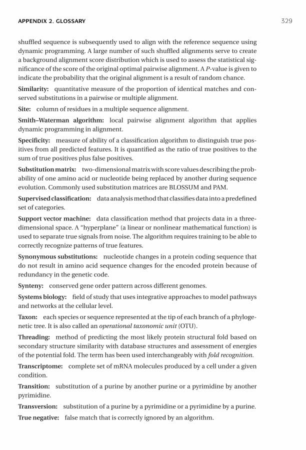
P1: JZP0521840988apx2 CB1022/Xiong 0 521 84098 8 January 10, 2006 13:15
APPENDIX 2. GLOSSARY 329
shuffled sequence is subsequently used to align with the reference sequence usingdynamic programming. A large number of such shuffled alignments serve to createa background alignment score distribution which is used to assess the statistical sig-nificance of the score of the original optimal pairwise alignment. A P-value is given toindicate the probability that the original alignment is a result of random chance.
Similarity: quantitative measure of the proportion of identical matches and con-served substitutions in a pairwise or multiple alignment.
Site: column of residues in a multiple sequence alignment.
Smith–Waterman algorithm: local pairwise alignment algorithm that appliesdynamic programming in alignment.
Specificity: measure of ability of a classification algorithm to distinguish true pos-itives from all predicted features. It is quantified as the ratio of true positives to thesum of true positives plus false positives.
Substitution matrix: two-dimensional matrix with score values describing the prob-ability of one amino acid or nucleotide being replaced by another during sequenceevolution. Commonly used substitution matrices are BLOSSUM and PAM.
Supervised classification: data analysis method that classifies data into a predefinedset of categories.
Support vector machine: data classification method that projects data in a three-dimensional space. A “hyperplane” (a linear or nonlinear mathematical function) isused to separate true signals from noise. The algorithm requires training to be able tocorrectly recognize patterns of true features.
Synonymous substitutions: nucleotide changes in a protein coding sequence thatdo not result in amino acid sequence changes for the encoded protein because ofredundancy in the genetic code.
Synteny: conserved gene order pattern across different genomes.
Systems biology: field of study that uses integrative approaches to model pathwaysand networks at the cellular level.
Taxon: each species or sequence represented at the tip of each branch of a phyloge-netic tree. It is also called an operational taxonomic unit (OTU).
Threading: method of predicting the most likely protein structural fold based onsecondary structure similarity with database structures and assessment of energiesof the potential fold. The term has been used interchangeably with fold recognition.
Transcriptome: complete set of mRNA molecules produced by a cell under a givencondition.
Transition: substitution of a purine by another purine or a pyrimidine by anotherpyrimidine.
Transversion: substitution of a purine by a pyrimidine or a pyrimidine by a purine.
True negative: false match that is correctly ignored by an algorithm.
P1: JZP0521840988apx2 CB1022/Xiong 0 521 84098 8 January 10, 2006 13:15
330 APPENDIX 2. GLOSSARY
True positive: true match that is correctly identified by an algorithm.
Unsupervised classification: data analysis method that does not assume predefinedcategories, but identifies data categories according to actual similarity patterns. It isalso called clustering.
UPGMA (unweighted pair-group method with arithmetic means): phylogenetictree-building method that involves clustering taxa based on phylogenetic distances.The method assumes the taxa to have equal distance from the root and starts treebuilding by clustering the two most closely related taxa. This produces a reducedmatrix, which allows the next nearest taxa to be added. Other taxa are sequentiallyadded using the same principle.
Z-score: statistical measure of the distance of a value from the mean of a scoredistribution, measured as the number of standard deviations.
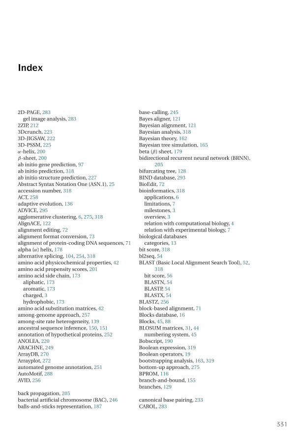
P1: KsF0521840988Ind CB1022/Xiong 0 521 84098 8 January 10, 2006 15:21
Index
2D-PAGE, 283gel image analysis, 283
2ZIP, 2123Dcrunch, 2233D-JIGSAW, 2223D-PSSM, 225α-helix, 200β-sheet, 200ab initio gene prediction, 97ab initio prediction, 318ab initio structure prediction, 227Abstract Syntax Notation One (ASN.1), 25accession number, 318ACT, 258adaptive evolution, 136ADVICE, 295agglomerative clustering, 6, 275, 318AlignACE, 122alignment editing, 72alignment format conversion, 73alignment of protein-coding DNA sequences, 71alpha (α) helix, 178alternative splicing, 104, 254, 318amino acid physicochemical properties, 42amino acid propensity scores, 201amino acid side chain, 173
aliphatic, 173aromatic, 173charged, 3hydrophobic, 173
amino acid substitution matrices, 42among-genome approach, 257among-site rate heterogeneity, 139ancestral sequence inference, 150, 151annotation of hypothetical proteins, 252ANOLEA, 220ARACHNE, 249ArrayDB, 270Arrayplot, 272automated genome annotation, 251AutoMotif, 288AVID, 256
back propagation, 205bacterial artificial chromosome (BAC), 246balls-and-sticks representation, 187
base-calling, 245Bayes aligner, 121Bayesian alignment, 121Bayesian analysis, 318Bayesian theory, 162Bayesian tree simulation, 165beta (β) sheet, 179bidirectional recurrent neural network (BRNN),
205bifurcating tree, 128BIND database, 293BioEdit, 72bioinformatics, 318
applications, 6limitations, 7milestones, 3overview, 3relation with computational biology, 4relation with experimental biology, 7
biological databasescategories, 13
bit score, 318bl2seq, 54BLAST (Basic Local Alignment Search Tool), 52,
318bit score, 56BLASTN, 54BLASTP, 54BLASTX, 54
BLASTZ, 256block-based alignment, 71Blocks database, 16Blocks, 45, 88BLOSUM matrices, 31, 44
numbering system, 45Bobscript, 190Boolean expression, 319Boolean operators, 19bootstrapping analysis, 163, 319bottom-up approach, 275BPROM, 116branch-and-bound, 155branches, 129
canonical base pairing, 233CAROL, 283
331
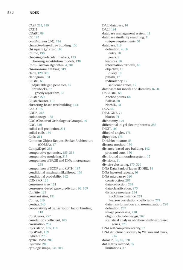
P1: KsF0521840988Ind CB1022/Xiong 0 521 84098 8 January 10, 2006 15:21
332 INDEX
CASP, 228, 319CATHCDART, 89CE, 195centiMorgan (cM), 244character-based tree building, 150chi square (χ2) test, 166Chime, 190choosing molecular markers, 133
choosing substitution models, 138Chou-Fasman algorithm, 4, 201chromosome walking, 319clade, 129, 319cladogram, 131Clustal, 65
adjustable gap penalties, 67drawbacks, 67
greedy algorithm, 67Cluster, 278ClusterBuster, 119clustering-based tree building, 143Cn3D, 190CODA, 218codon usage, 135COG (Cluster of Orthologous Groups), 90COG, 319coiled coil prediction, 211coiled coils, 180Coils, 211Common Object Request Broker Architecture
(CORBA), 17Comp2Dgel, 283comparative genomics, 255, 319comparative modeling, 215comparison of SAGE and DNA microarrays,
278comparison of SCOP and CATH, 197conditional maximum likelihood, 108conditional probability, 162CONPRO, 120consensus tree, 131consensus-based gene prediction, 98, 109ConSite, 121constant sites, 151Contig, 319contigs, 246cooperativity of transcription factor binding,
118CoreGenes, 257correlation coefficient, 103covariation, 237CpG island, 105, 118CpGProD, 119Cyber-T, 273cyclic HMM, 206Cysteine, 288cytologic maps, 244, 319
DALI database, 16DALI, 194database management system, 11database similarity searching, 51
unique requirements, 51database, 319
definition, 4, 10entry, 10goals, 5
features, 10information retrieval, 18objective, 10
query, 10pitfalls, 17redundancy, 17
sequence errors, 17databases for motifs and domains, 87–89DbClustal, 68
Anchor points, 68Ballast, 68NorMD, 68
DCA, 64DIALIGN2, 71
blocks, 71dichotomy, 129differential in-gel electrophoresis, 285DIGIT, 109dihedral angles, 175dipeptide, 175Dirichlet mixture, 83discrete method, 150distance-based tree building, 142
pros and cons, 150distributed annotation system, 17divisions, 21divisive clustering, 275, 320DNA Data Bank of Japan (DDBJ), 14DNA inverted repeats, 36DNA microarray, 320
construction, 267data collection, 269data classification, 273distance measure, 274
Euclidean distance, 274Pearson correlation coefficients, 274
data transformation and normalization, 270definition, 267image processing, 270oligonucleotide design, 267statistical analysis of differentially expressed
genes, 273DNA self complementarity, 37DNA structure discovery by Watson and Crick,
214domain, 35, 85, 320dot matrix method, 35
limitations, 37

P1: KsF0521840988Ind CB1022/Xiong 0 521 84098 8 January 10, 2006 15:21
INDEX 333
dot plot, 320Dothelix, 37Dotmatcher, 37Dottup, 37double dynamic programming, 195Dustin units, 245Dynalign, 238dynamic programming, 37, 320
EGAD database, 263electrospray ionization MS, 284eletrostatic interaction, 177EM, 320EMBOSS package, 37emission probability, 80Emotif, 87energy minimization, 219Entrez, 18, 19EPCLUST, 278Eponine, 119erroneous annotation, 18EST, 320EST2Genome, 108eukaryotic ab initio gene prediction, 105
based on gene signals, 105based on gene content, 105
eukaryotic gene organization, 103eukaryotic genome structure, 103EULER, 249Eulerian superpath, 249European Bioinformatics Institute (EBI),
16European Molecular Biology Laboratory
(EMBL), 14E-value, 55, 320evolution, definition, 127evolutionary models, 138exact matching, 86exhaustive database searching, 51exhaustive method, 64
dynamic programming, 64heuristic method, 65
exhaustive tree searching, 152exon shuffling, 254, 320exons, 103EXPASY, 285
AACompIdent, 285CombSearch, 285FindMod, 288GlyMod, 289PepIdent, 285TagIdent, 285
expectation maximization (EM), 91, 122local optimum, 91
expressed sequence tags (ESTs), 261clustering process, 263databases, 262
drawbacks, 262index construction, 262
eXtensible Markup Language (XML), 17
false negative, 102, 321false positives, 51, 102, 321FASTA format, 23FASTA, 57, 321
FASTX, 59statistical significance, 60
FGENES, 107FGENESB, 68field values, 10field, 10FindTerm, 118fingerprints, 88, 321finishing phase of genome sequencing, 245FirstEF, 119Fitch-Margolish method, 149fixed-order Markov model, 100flat file format, 10
delimiter, 10flat file, 321flexible substitution matrices, 67
weighting scheme, 67fold recognition, 321fold, 321Foldalign, 238FootPrinter, 121for nucleotide sequences, 41forensic DNA analysis, 6forward algorithm, 82forward-reverse constraint, 248fossil records, 127Fourier transform, 181FREAD, 218Fugue, 227functional genomics, 243, 321
using sequence-based approaches, 261using microarray-based approaches, 267
fuzzy matching, 87
gamma (γ ) distribution, 140gap penalty, 38, 321
affine, 38constant, 38
GAP program, 40GC skew, 258GenBank, 4, 14, 21
accession number, 21gene annotation, 321gene collinearity, 259gene content, 97gene index (gi) number, 22gene number in human genome, 253gene ontology, 18, 250, 321
controlled vocabulary, 250

P1: KsF0521840988Ind CB1022/Xiong 0 521 84098 8 January 10, 2006 15:21
334 INDEX
gene order comparison, 258gene phylogeny, 130gene prediction, 97
performance evaluation, 102, 109gene signals, 97GeneComber, 109GeneMark, 102
GeneMarkS, 102GeneMark heuristic, 102
GeneOrder, 259GeneQuiz, 252generalized neighbor-joining, 145genetic algorithm, 161, 321
crossing, 161fitness, 161offspring, 161
genetic diversity, 127genetic linkage maps, 243genetic map, 243, 322genetic markers, 243genome annotation, 250genome economy, 254genome mapping, 243genome sequence assembly, 246genome, 322GenomeScan, 108GenomeVista, 256genomics, 243, 322GenPept, 21GENSCAN, 107GenThreader, 227Gibbs motif sampling, 91, 122Gibbs sampling, 322Glimmer, 102
GlimmerM, 102Global alignment, 34, 322global minimum, 219global tree searching, 156globular proteins, 180Gonnet matrices, 46GOR method, 202Grail, 106graphical output box, 57
color coding, 57Grasp, 190GROMOS, 219GT-AG rule, 105Gumble extreme value distribution, 47
hashing, 57heuristic database searching, 51heuristic tree searching, 156heuristics, 322hidden Markov model, 80, 322
applications, 83hierarchical clustering, 275, 322
average linkage method, 276
complete linkage method, 276single linkage method, 276
hierarchical genome sequencing approach, 245,322
high-scoring segment pair (HSP), 53HMMer, 83HMMgene, 108HMMSTR, 206homologous relationships, 32homologs, 322homology modeling, 215, 323
backbone model building, 217loop modeling, 217
ab initio method, 217database method, 217
model evaluation, 220based on physicalchemical rules, 220based on statistical profiles, 220
model refinement, 219sequence alignment, 216side chain refinement, 218template selection, 215
homology, 322homology-based gene prediction, 98, 108homoplasy, 137, 323horizontal gene transfer, 257HSP, 323hydrogen bond, 177
identity, 323Immunoglobulin BLAST, 54INCLUSive, 123informative sites, 151initiator sequence, 115integral membrane proteins, 180intensity-ratio plot, 272interologs, 293interpolated Markov model, 101InterPreTS, 293InterPro, 89introns, 104
splicing, 104IPPRED, 293iPSORT, 290iterative multiple alignment, 69
jackknifing, 165, 323JPRED, 207JTT (Jones-Taylor-Thorton) matrices,
46Jukes-Cantor model, 138, 323jury network, 205
Kimura model, 138, 323Kishino-Hasegawa test, 166k-means clustering, 276, 323
centroid value, 277
P1: KsF0521840988Ind CB1022/Xiong 0 521 84098 8 January 10, 2006 15:21
INDEX 335
Kozak sequence, 105ktuples, 57
LAGAN, 256LALIGN, 41lateral gene transfer, 257
conjugation, 257transduction, 257transformation, 257
lateral gene transfer, 323leucine zipper domain, 212lineage, 129linear discriminant analysis (LDA), 102, 107,
323local alignment, 34, 323local minimum, 156, 219log-odds score, 43, 324long-branch attraction, 157
solutions, 158loops, 179low complexity region (LCR), 56, 324Lowess regression, 272
MA-ANOVA, 273machine learning, 324macromolecular crystallographic information
file (mmCIF), 184Margaet Dayhoff, 3Markov chain Monte Carlo procedure, 162Markov model, 79, 324
orders, 80Mascot, 285masking, 56
hard, 56soft, 56
mass spectrometry (MS), 284Match-Box, 71Matrix, 295matrix-assisted laser desorption ionization
(MALDI) MS, 284MatrixPlot, 37MAVID, 256maximum likelihood, 166, 324
pros and cons, 160maximum parsimony, 150, 324
assumption, 150pros and cons, 156
McPromoter, 119Melanie, 283Melina, 122MEME, 92, 122MeSH system, 19Mfold, 236midnight zone, 33midpoint rooting, 130minimal genome, 257minimum evolution, 149, 324
mirror-tree method, 294missed exons, 110missed genes, 110ModBase, 223Modeller, 222molecular clock, 130, 324molecular dynamic simulation, 219molecular fossils, 31, 128molecular modeling database (MMDB) file, 185molecular phylogenetics, 128, 324
assumptions, 128molecular replacement, 181Molscript, 189monomer, 177monophyletic group, 129Monophyletic, 324Monte Carlo procedure, 324motifs, 35, 85, 324
based on multiple alignment, 86based on statistical models, 87
MrBayes, 168Multicoil, 212multifurcating node, 129, 132Multi-LAGAN, 256MultiPipMaker, 256multiple isomorphous replacement, 181multiple sequence alignment, 63
advantage, 63multiple structure alignment, 194multiple substitutions, 137MUMmer, 256mutation, 161MZEF, 107
National Center for Biotechnology Information(NCBI), 18
natural selection, 127NCBI taxonomy database, 20nearest neighbor interchange, 156Needleman-Wunsch algorithm, 4, 40, 324negative selection, 136, 324neighbor joining, 143, 325neural network, 106, 204, 325Newick format, 131, 325NJML, 161node, 129noncanonical base pairing, 233non-informative sites, 151non-parametric bootstrapping, 163nonsynonymous substitutions, 136, 325NorMD, 137nuclear magnetic resonance (NMR)
spectroscopy, 181null hypothesis, 273
object-oriented database, 12, 325pointer, 12
P1: KsF0521840988Ind CB1022/Xiong 0 521 84098 8 January 10, 2006 15:21
336 INDEX
object-relational database management system,13
Occam’s razor, 150OligoArray, 269OligoWiz, 269Online Mendelian Inheritance in Man (OMIM),
20, 325open reading frames (ORF), 98operational taxonomic unit (OTU), 129operon, 116operon prediction, 116optimality-based tree building, 149orthologs, 325outgroup, 130, 325overfitting, 83, 325
pairwise sequence alignment, 31PAM matrices, 43, 325
construction, 43multiple substitutions, 44unit, 44
ParAlign, 61paralogs, 326parametric bootstrapping, 163paraphyletic, 129PAUP, 167PDB, 14peptide bond, 174peptide plane, 175peptide, 175personlized medicine, 7PETRA, 218Pfam database, 16Pfam, 88phases of crystal diffraction, 181PHD, 205phi (φ) angle, 175Phobius, 210Phrap, 249Phred, 249Phylip, 167PhyloCon, 123phylogenetic analysis procedure, 133
alignment, 136phylogenetic footprinting, 326phylogenetic footprints, 120phylogenetic profile, 293, 326phylogenetic tree evaluation, 163phylogenetics, 127phylogeny, 127, 326phylogram, 131PHYML, 168physical maps, 326, 244PipMaker, 256Poa, 68polypeptide, 175
C-terminus, 175
backbone atoms, 175N-terminus, 175
Polyphobius, 210polytomy, 129PORTER, 205position-specific scoring matricies (PSSM), 75
construction, 75positive selection, 136, 326positive-inside rule, 209posterior probability, 162, 326posttranslational modifications, 174, 287
prediction, 287PRALINE, 69, 137prediction of disulfide bonds, 288prediction of protein subcellular locations,
290PredictProtein, 207primary database, 14Prints, 88Procheck, 220ProDom, 88PROF, 206profile, 69, 78, 326ProFound, 285progressive alignment, 326progressive multiple alignment, 65
guide tree, 65prokaryotic gene prediction
based on codon biase, 99based on hidden Markov models, 100based on Markov models, 100
prokaryotic genome structure, 98PromH(W), 121promoter elements, 113
prokaryotic, 113eukaryotic, 114
promoter prediction, 113difficulty, 113ab initio method, 115
eukaryotic, 118prokaryotic, 116
based on phylogenetic footing, 120based on expression profiles, 122
Prosite, 87pitfalls, 87
ProSplicer, 255PROTA2DNA, 72Protein Data Bank (PDB), 3, 182
format, 183ATOM field, 183HETATM field, 183
protein family, 327protein microarrays, 285
antibody-based, 286protein-print, 287protein-scaffolds, 286
protein primary structure, 176
P1: KsF0521840988Ind CB1022/Xiong 0 521 84098 8 January 10, 2006 15:21
INDEX 337
protein quaternary structure, 176protein secondary structure for globular
proteins, 201ab initio method, 201first-generation methods, 203homology-based methods, 203prediction accuracy, 207second-generation methods, 203third-generation methods, 203with neural networks, 204
protein secondary structure for transmembraneproteins, 208
prediction of helical membrane proteins, 209prediction of β-barrel membrane proteins,
210protein secondary structure prediction,
definition of, 200protein secondary structure, 176protein sorting, 289protein structure classification, 195
procedure, 196protein structure comparison
applications, 191hybrid method, 194intermolecular method, 191
iterative optimization, 193rotation, 191superimposition, 191translation, 191
intramolecular method, 193distance matrix, 194
protein structure modeling, applications of,214
protein structure native state, 227protein structure visualization, 187protein supersecondary structure, 177protein targeting, 289protein tertiary structure, 176protein-protein interactions determination
using the yeast two-hybrid method, 291drawbacks
using affinity purification techniques, 291protein-protein interactions prediction, 292
based on domain fusion, 292based on gene neighbors, 293based on phylogenetic information, 293based on sequence homology, 293
proteome analysis procedure, 281proteome, 281, 327proteomics, 281, 327
advantages over functional genomics,281
ProtoNet, 91PRRN, 70PRSS, 48pseudocounts, 83psi (ψ) angle, 175
PSI-BLAST, 78, 327weighting scheme, 78profile drift, 79pseudocounts, 79
PSIPRED, 205PSORT, 290PSSM, 327PubMed, 19
field tags, 20purifying selection, 136P-value, 327
quadratic discriminant analysis (QDA), 107,327
qualifiers, 23quantitative tool use, 3quartet puzzling, 160, 327quartets, 160query, 327
radiation, 129Ramachandran plot, 175, 327random coils, 179Rascal, 73, 137RasMol, 188RasTop, 188rational drug design, 6RBSfinder, 102Readseq, 25, 73RefSeq, 18Regular expression, 86, 328
rules, 86regularization, 83regulatory elements, 114relational database, 11, 32
table, 11RepeatMasker, 56representing multiple sequence alignment,
81RESID, 289Reverse PSI-BLAST (RPS-BLAST), 89RevTrans, 72R-factor, 181Rho (ρ)-independent terminator, 98ribbons representation, 187Ribbons, 190RMSD (root mean square deviation), 191, 327RMSD100, 193RNA forms, 231RNA functions, 231RNA primary structure, 233RNA secondary structure prediction
ab initio approach, 234free energy calculation, 234cooperativity in helix formation, 234destabilizing force in helix formation,
235
P1: KsF0521840988Ind CB1022/Xiong 0 521 84098 8 January 10, 2006 15:21
338 INDEX
RNA secondary structure prediction (cont.)dot matrix method, 235dynamic programming, 235partition function, 236
comparative approach, 237algorithms that use prealignment, 238algorithms that do not use prealignment,
238performance evaluation, 239
RNA secondary structure, 233bulge loop, 233hairpin loop, 233helical junctions, 233interior loop, 233multibranch loop, 233
RNA supersecondary structure, 234hairpin bulge, 234kissing hairpin, 234pseudoknot loop, 234
RNA tertiary structure, 233RNAalifold, 238RNAfold, 236root node, 129rooted tree, 130Rosetta stone method, 292Rossetta, 228rotamer library, 218, 328rotamer, 218, 328r-value, 143rVISTA, 121
safe zone, 33SAGE Genie, 267SAGEmap, 267SAGExProfiler, 267scaffolds, 246, 328scaled tree, 131ScanAlyze, 270ScanPS, 61SCOP, 196score computation, 82scoring function, 63
sum-of-pairs, 63SCWRL, 219secondary database, 14SEG, 56self-organizing map, 277, 328sensitivity, 51, 103, 328sequence alignment, 31
evolutionary basis, 31statistical significance 47
sequence format, 21sequence homology, 32sequence identity, 33sequence logos, 92, 328Sequence Retrieval Systems (SRS), 18,
25
sequence similarity, 32, 33, 329serial analysis of gene expression (SAGE),
264, 328drawbacks, 265tags, 264
SGP-1, 109Shimodaira-Hasegawa test, 166Shine-Dalgarno sequence, 98shotgun sequencing, 245, 328shuffle test, 47, 328
P-value, 48sigma (σ ) subunit, 113signal sequences, 289SignalP, 290signature indel, 137SIM, 41sister taxa, 129site, 329SMART, 89Smith–Waterman algorithm, 40, 329SNOMAD, 273SOTA, 278space-filling representation, 187specialized database, 14, 16species phylogeny, 130specificity, 51, 103, 329speed, 51spliceosome, 104SSAP, 195SSEARCH, 41SSPRO, 205STAMP, 195star decomposition, 145statistical models for multiple sequence
alignment, 75statistical significance, 55Stephen Altschul, 4STRING, 295structural fold recognition, 223structural genomics, 243structural profiles, 224structural proteomics, 243structured query language, 11Student t-test, 166Substitution matrix, 41, 329
based on empirical rules, 42based on genetic code, 42based on interchangeability, 42based on physicochemical properties, 42for amino acid sequences, 41
substitution models, 138subtree pruning and regrafting, 156subunit, 177supercontigs, 246supervised classification, 275, 329support vector machine (SVM), 210, 287, 329
hyperplane, 288

P1: KsF0521840988Ind CB1022/Xiong 0 521 84098 8 January 10, 2006 15:21
INDEX 339
Swaap, 258SWISS-2DPAGE, 283Swiss-Model, 222Swiss-PDBViewer, 189SWISS-PROT, 15synonymous substitutions, 136, 329synteny, 258, 329systems biology, 8, 329
tandem mass spectrometry, 284TargetP, 290TATA box, 115taxa (taxon), 129, 329TBBpred, 210TBLASTN, 54TBLASTX, 54T-Coffee, 68
library extension, 68TESTCODE, 99TFASTX, 59threading, 223, 329
pairwise energy method, 224double dynamic programming,
224profile method, 224
TIGR Assembler, 249TIGR Gene Indices, 263
tentative consensus (TC), 263TIGR Spotfinder, 270TIGR TM4, 278TMHMM, 210top-down approach, 275tortional angle, 175training, 80transcription factors, 114transcriptome analysis, 261transcriptome, 329TRANSFAC, 121transformed r-value, 143transitional probability, 79, 80transitions, 41, 329transversions, 41, 329traveling salesman problem, 249Tree of Life, 121
tree topology, 129tree-bisection and reconnection, 156TREE-PUZZLE, 167TrEMBL, 15true negative, 102, 329true positives, 51, 102, 330TSSW, 119tuple, 36twilight zone, 33TwinScan, 109
UniGene cluster, 263UniGene database, 263UniGene, 18UniProt, 16unrooted tree, 129unscaled tree, 131unsupervised classification, 275, 330UPGMA, 143, 330
assumption, 143
Van der Waals force, 177VAST, 195VecScreen, 54, 249Verify3D, 220Viterbi algorithm, 82
WebLogo, 93WebMol, 190WebPhylip, 167weighted parsimony, 152WHAT IF, 220whole genome alignment, 255William Pearson, 4window, 36wire-frame representation, 187within-genome approach, 257word method for pairwise alignment, 52wrong genes, 110wrongly predicted exons, 110
x-ray crystallography, 181
Z-score, 194, 330

P1: KsF0521840988Ind CB1022/Xiong 0 521 84098 8 January 10, 2006 15:21
340

P1: KsF0521840988plt CB1022/Xiong 0 521 84098 8 January 10, 2006 14:8
Figure 9.1. Schematic representation of elements involved in bacterial transcription initiation. RNApolymerase binds to the promoter region, which initiates transcription through interaction with tran-scription factors binding at different sites. Abbreviations: TSS, transcription start site; ORF, readingframe; pol, polymerase; TF, transcription factor (see page 114).
Figure 9.2. Schematic diagram of an eukaryotic promoter with transcription factors and RNA po-lymerase bound to the promoter. Abbreviations: Inr, initiator sequence; ORF, reading frame; pol, po-lymerase; TF, transcription factor (see page 115).
Figure 12.3. Definition of dihedral angles of φ and ψ. Six atoms around a peptide bond forming apeptide plane are colored in red. The φ angle is the rotation about the N–Cα bond, which is measuredby the angle between a virtual plane formed by the C–N–Cα and the virtual plane by N–Cα–C (C ingreen). The ψ angle is the rotation about the Cα–C bond, which is measured by the angle betweena virtual plane formed by the N–Cα–C (N in green) and the virtual plane by Cα–C–N (N in red) (seepage 176).
1
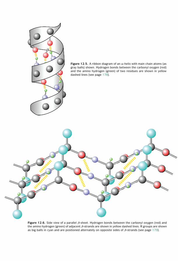
P1: KsF0521840988plt CB1022/Xiong 0 521 84098 8 January 10, 2006 14:8
Figure 12.5. A ribbon diagram of an α-helix with main chain atoms (asgray balls) shown. Hydrogen bonds between the carbonyl oxygen (red)and the amino hydrogen (green) of two residues are shown in yellowdashed lines (see page 178).
Figure 12.6. Side view of a parallel β-sheet. Hydrogen bonds between the carbonyl oxygen (red) andthe amino hydrogen (green) of adjacent β-strands are shown in yellow dashed lines. R groups are shownas big balls in cyan and are positioned alternately on opposite sides of β-strands (see page 179).
2

P1: KsF0521840988plt CB1022/Xiong 0 521 84098 8 January 10, 2006 14:8
Figure 13.1. Examples of molecular structure visualization forms. (A) Wireframes. (B) Balls and sticks.(C) Space-filling spheres. (D) Ribbons (see page 188).
3
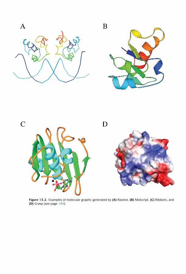
P1: KsF0521840988plt CB1022/Xiong 0 521 84098 8 January 10, 2006 14:8
Figure 13.2. Examples of molecular graphic generated by (A) Rasmol, (B) Molscript, (C) Ribbons, and(D) Grasp (see page 189).
4

P1: KsF0521840988plt CB1022/Xiong 0 521 84098 8 January 10, 2006 14:8
Figure 17.4. Example of sequence assembly with or without applying forward–reverse constraint, whichfixes the sequence distance from both ends of a subclone. Without the restraint, the red fragment ismisassembled due to matches of repetitive element in the middle of a fragment (see page 248).
5
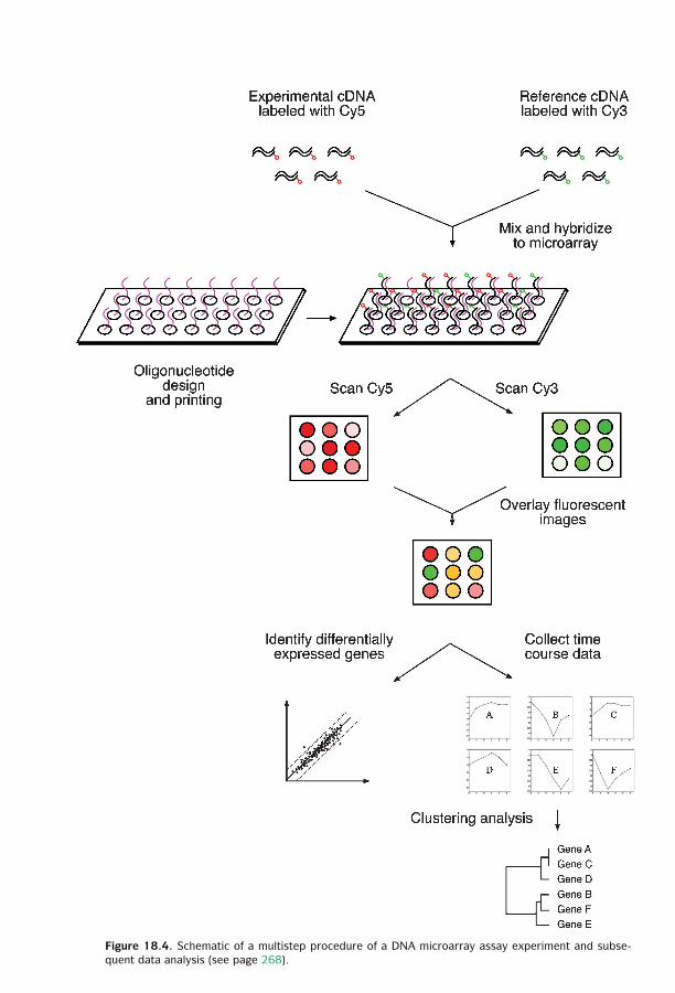
P1: KsF0521840988plt CB1022/Xiong 0 521 84098 8 January 10, 2006 14:8
Figure 18.4. Schematic of a multistep procedure of a DNA microarray assay experiment and subse-quent data analysis (see page 268).
6
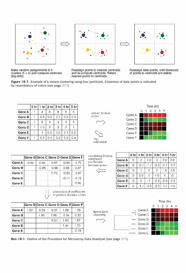
P1: KsF0521840988plt CB1022/Xiong 0 521 84098 8 January 10, 2006 14:8
Figure 18.7. Example of k-means clustering using four partitions. Closeness of data points is indicatedby resemblance of colors (see page 277).
Box 18.1. Outline of the Procedure for Microarray Data Ananlysis (see page 271).
7
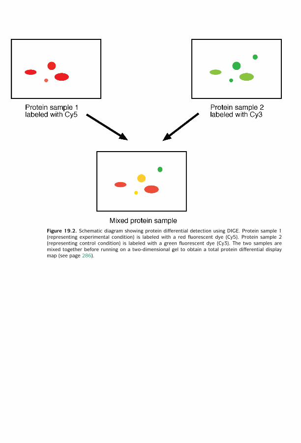
P1: KsF0521840988plt CB1022/Xiong 0 521 84098 8 January 10, 2006 14:8
Figure 19.2. Schematic diagram showing protein differential detection using DIGE. Protein sample 1(representing experimental condition) is labeled with a red fluorescent dye (Cy5). Protein sample 2(representing control condition) is labeled with a green fluorescent dye (Cy3). The two samples aremixed together before running on a two-dimensional gel to obtain a total protein differential displaymap (see page 286).
8