Fluid Mechanics Kundu Cohen 6th edition solutions Sm ch (2)

Fluid Mechanics, 6th Ed. Kundu, Cohen, and Dowling

Exercise 2.1. For three spatial dimensions, rewrite the following expressions in index notation and evaluate or simplify them using the values or parameters given, and the definitions of δij and εijk wherever possible. In b) through e), x is the position vector, with components xi. a)

€

b ⋅ c where b = (1, 4, 17) and c = (–4, –3, 1) b)

€

u ⋅ ∇( )x where u a vector with components ui. c)

€

∇φ , where

€

φ = h ⋅ x and h is a constant vector with components hi. d)

€

∇ ×u, where u = Ω × x and Ω is a constant vector with components Ωi.

e)

€

C ⋅ x , where

€

C =

1 2 30 1 20 0 1

"

# $

% $

&

' $

( $

Solution 2.1. a)

€

b ⋅ c = bici =1(−4) + 4(−3) +17(1) = −4 −12 +17 = +1

b)

€

u ⋅ ∇( )x = u j∂∂x j

xi = u1∂∂x1

%

& '

(

) * + u2

∂∂x2

%

& '

(

) * + u3

∂∂x3

%

& '

(

) *

+

, -

.

/ 0

x1x2x3

+

,

- - -

.

/

0 0 0

€

=

u1∂x1∂x1

#

$ %

&

' ( + u2

∂x1∂x2

#

$ %

&

' ( + u3

∂x1∂x3

#

$ %

&

' (

u1∂x2∂x1

#

$ %

&

' ( + u2

∂x2∂x2

#

$ %

&

' ( + u3

∂x2∂x3

#

$ %

&

' (

u1∂x3∂x1

#

$ %

&

' ( + u2

∂x3∂x2

#

$ %

&

' ( + u3

∂x3∂x3

#

$ %

&

' (

)

*

+ + + + + + +

,

-

.

.

.

.

.

.

.

=

u1 ⋅1+ u2 ⋅ 0 + u3 ⋅ 0u1 ⋅ 0 + u2 ⋅1+ u3 ⋅ 0u1 ⋅ 0 + u2 ⋅ 0 + u3 ⋅1

)

*

+ + +

,

-

.

.

.

= u jδij =

u1u2u3

)

*

+ + +

,

-

.

.

.

= ui

c)

€

∇φ =∂φ∂x j

=∂∂x j

hixi( ) = hi∂xi∂x j

= hiδij = h j = h

d)

€

∇ ×u =∇ × Ω × x( ) = εijk∂∂x j

εklmΩl xm( ) = εijkεklmΩlδ jm = δilδ jm −δimδ jl( )Ωlδ jm = δilδ jj −δijδ jl( )Ωl

€

= 3δil −δil( )Ωl = 2δilΩl = 2Ωl = 2Ω Here, the following identities have been used:

€

εijkεklm = δilδ jm −δimδ jl ,

€

δijδ jk = δik ,

€

δ jj = 3, and

€

δijΩ j =Ωi

e)

€

C ⋅ x = Cij x j =

1 2 30 1 20 0 1

#

$ %

& %

'

( %

) %

x1x2x3

#

$ %

& %

'

( %

) %

=

x1 + 2x2 + 3x3x2 + 2x3x3

#

$ %

& %

'

( %

) %


Exercise 2.2. Starting from (2.1) and (2.3), prove (2.7). Solution 2.2. The two representations for the position vector are:

€

x = x1e1 + x2e2 + x3e3 , or

€

x = " x 1 " e 1 + " x 2 " e 2 + " x 3 " e 3 . Develop the dot product of x with e1 from each representation,

€

e1 ⋅ x = e1 ⋅ x1e1 + x2e2 + x3e3( ) = x1e1 ⋅ e1 + x2e1 ⋅ e2 + x3e1 ⋅ e3 = x1 ⋅1+ x2 ⋅ 0 + x3 ⋅ 0 = x1 , and

€

e1 ⋅ x = e1 ⋅ # x 1 # e 1 + # x 2 # e 2 + # x 3 # e 3( ) = # x 1e1 ⋅ # e 1 + # x 2e1 ⋅ # e 2 + # x 3e1 ⋅ # e 3 = # x iC1i , set these equal to find:

€

x1 = " x iC1i , where

€

Cij = e i ⋅ # e j is a 3 × 3 matrix of direction cosines. In an entirely parallel fashion, forming the dot product of x with e2, and x with e2 produces:

€

x2 = " x iC2i and

€

x3 = " x iC3i . Thus, for any component xj, where j = 1, 2, or 3, we have:

€

x j = " x iC ji , which is (2.7).


Exercise 2.3. For two three-dimensional vectors with Cartesian components ai and bi, prove the Cauchy-Schwartz inequality: (aibi)2 ≤ (ai)2(bi)2. Solution 2.3. Expand the left side term,

(aibi )2 = (a1b1 + a2b2 + a3b3)

2 = a12b1

2 + a22b2

2 + a32b3

2 + 2a1b1a2b2 + 2a1b1a3b3 + 2a2b2a3b3 , then expand the right side term,

(ai )2 (bi )

2 = (a12 + a2

2 + a32 )(b1

2 + b22 + b3

2 ) = a1

2b12 + a2

2b22 + a3

2b32 + (a1

2b22 + a2

2b12 )+ (a1

2b32 + a3

2b12 )+ (a3

2b22 + a2

2b32 ).

Subtract the left side term from the right side term to find: (ai )

2 (bi )2 − (aibi )

2

= (a12b2

2 − 2a1b1a2b2 + a22b1

2 )+ (a12b3

2 − 2a1b1a3b3 + a32b1

2 )+ (a32b2

2 − 2a2b2a3b3 + a22b3

2 )

= (a1b2 − a2b1)2 + (a1b3 − a3b1)2 + (a3b2 − a2b3)2 = a×b 2 .

Thus, the difference (ai )2 (bi )

2 − (aibi )2 is greater than zero unless a = (const.)b then the

difference is zero.


Exercise 2.4. For two three-dimensional vectors with Cartesian components ai and bi, prove the triangle inequality: a + b ≥ a+b . Solution 2.4. To avoid square roots, square both side of the equation; this operation does not change the equation's meaning. The left side becomes:

a + b( )2= a 2 + 2 a b + b 2 ,

and the right side becomes: a+b 2

= (a+b) ⋅ (a+b) = a ⋅a+ 2a ⋅b+b ⋅b = a 2 + 2a ⋅b+ b 2 . So,

a + b( )2− a+b 2

= 2 a b − 2a ⋅b . Thus, to prove the triangle equality, the right side of this last equation must be greater than or equal to zero. This requires:

a b ≥ a ⋅b or using index notation: ai2bi

2 ≥ aibi , which can be squared to find:

ai2bi

2 ≥ (aibi )2 ,

and this is the Cauchy-Schwartz inequality proved in Exercise 2.3. Thus, the triangle equality is proved.


Exercise 2.5. Using Cartesian coordinates where the position vector is x = (x1, x2, x3) and the fluid velocity is u = (u1, u2, u3), write out the three components of the vector:

€

u ⋅ ∇( )u = ui ∂u j ∂xi( ) . Solution 2.5.

a)

€

u ⋅ ∇( )u = ui∂u j

∂xi

%

& '

(

) * = u1

∂u j

∂x1

%

& '

(

) * + u2

∂u j

∂x2

%

& '

(

) * + u3

∂u j

∂x3

%

& '

(

) * =

u1∂u1∂x1

%

& '

(

) * + u2

∂u1∂x2

%

& '

(

) * + u3

∂u1∂x3

%

& '

(

) *

u1∂u2∂x1

%

& '

(

) * + u2

∂u2∂x2

%

& '

(

) * + u3

∂u2∂x3

%

& '

(

) *

u1∂u3∂x1

%

& '

(

) * + u2

∂u3∂x2

%

& '

(

) * + u3

∂u3∂x3

%

& '

(

) *

+

,

- - -

.

- - -

/

0

- - -

1

- - -

€

=

u ∂u∂x#

$ %

&

' ( + v

∂u∂y#

$ %

&

' ( + w

∂u∂z#

$ %

&

' (

u ∂v∂x#

$ %

&

' ( + v

∂v∂y#

$ %

&

' ( + w

∂v∂z#

$ %

&

' (

u ∂w∂x#

$ %

&

' ( + v

∂w∂y#

$ %

&

' ( + w

∂w∂z

#

$ %

&

' (

)

*

+ + +

,

+ + +

-

.

+ + +

/

+ + +

The vector in this exercise,

€

u ⋅ ∇( )u = ui ∂u j ∂xi( ) , is an important one in fluid mechanics. As described in Ch. 3, it is the nonlinear advective acceleration.


Exercise 2.6. Convert ∇×∇ρ to indicial notation and show that it is zero in Cartesian coordinates for any twice-differentiable scalar function ρ. Solution 2.6. Start with the definitions of the cross product and the gradient.

∇× ∇ρ( ) = εijk∂∂x j

∇ρ( )k = εijk∂ 2ρ∂x j∂xk

Write out the vector component by component recalling that εijk = 0 if any two indices are equal. Here the "i" index is the free index.

εijk∂ 2ρ∂x j∂xk

=

ε123∂ 2ρ∂x2∂x3

+ε132∂ 2ρ∂x3∂x2

ε213∂ 2ρ∂x1∂x3

+ε231∂ 2ρ∂x3∂x1

ε312∂ 2ρ∂x1∂x2

+ε321∂ 2ρ∂x2∂x1

!

"

####

$

####

%

&

####

'

####

=

∂ 2ρ∂x2∂x3

– ∂ 2ρ∂x3∂x2

– ∂ 2ρ∂x1∂x3

+∂ 2ρ∂x3∂x1

∂ 2ρ∂x1∂x2

−∂ 2ρ∂x2∂x1

!

"

####

$

####

%

&

####

'

####

= 0 ,

where the middle equality follows from the definition of εijk (2.18), and the final equality follows

when ρ is twice differentiable so that

€

∂ 2ρ∂x j∂xk

=∂ 2ρ∂xk∂x j

.


Exercise 2.7. Using indicial notation, show that a × (b × c) = (a ⋅ c)b − (a ⋅ b)c. [Hint: Call d ≡ b × c. Then (a × d)m = εpqmapdq = εpqmapεijqbicj. Using (2.19), show that (a × d)m = (a ⋅ c)bm − (a ⋅ b)cm.] Solution 2.7. Using the hint and the definition of εijk produces:

(a × d)m = εpqmapdq = εpqmapεijqbicj = εpqmεijq bicjap = –εijqεqpm bicjap. Now use the identity (2.19) for the product of epsilons:

(a × d)m = – (δipδjm – δimδpj) bicjap = – bpcmap + bmcpap. Each term in the final expression involves a sum over "p", and this is a dot product; therefore

(a × d)m = – (a ⋅ b)cm + bm(a ⋅ c). Thus, for any component m = 1, 2, or 3,

a × (b × c) = − (a ⋅ b)c + (a ⋅ c)b = (a ⋅ c)b − (a ⋅ b)c.


Exercise 2.8. Show that the condition for the vectors a, b, and c to be coplanar is εijkaibjck = 0. Solution 2.8. The vector b × c is perpendicular to b and c. Thus, a will be coplanar with b and c if it too is perpendicular to b × c. The condition for a to be perpendicular with b × c is:

a ⋅ (b × c) = 0. In index notation, this is aiεijkbjck = 0 = εijkaibjck.


Exercise 2.9. Prove the following relationships: δijδij = 3, εpqrεpqr = 6, and εpqiεpqj = 2δij. Solution 2.9. (i) δijδij = δii = δ11 + δ22 + δ33 = 1 + 1 + 1 = 3. For the second two, the identity (2.19) is useful. (ii) εpqrεpqr = εpqrεrpq = δppδqq – δpqδpq = 3(3) – δpp = 9 – 3 = 6. (iii) εpqiεpqj = εipqεpqj = – εipqεqpj = – (δipδpj – δijδpp) = – δij + 3δij = 2δij.


Exercise 2.10. Show that C⋅CT = CT⋅C = δ , where C is the direction cosine matrix and δ is the matrix of the Kronecker delta. Any matrix obeying such a relationship is called an orthogonal matrix because it represents transformation of one set of orthogonal axes into another. Solution 2.10. To show that C⋅CT = CT⋅C = δ , where C is the direction cosine matrix and δ is the matrix of the Kronecker delta. Start from (2.5) and (2.7), which are

€

" x j = xiCij and

€

x j = " x iC ji , respectively, and change the index "i" into "m" on (2.5):

€

" x j = xmCmj . Substitute this into (2.7) to find:

€

x j = " x iC ji = xmCmi( )C ji = CmiC jixm . However, we also have xj = δjmxm, so

€

δ jm xm = CmiC jixm → δ jm = CmiC ji, which can be written:

€

δ jm = CmiCijT = C⋅CT,

and taking the transpose of the this produces:

€

δ jm( )T

= δmj = CmiCijT( )

T= Cmi

TCij = CT⋅C.


Exercise 2.11. Show that for a second-order tensor A, the following quantities are invariant under the rotation of axes:

I1 = Aii , I2 =A11 A12A21 A22

+A22 A23A32 A33

+A11 A13A31 A33

, and I3 = det(Aij).

[Hint: Use the result of Exercise 2.8 and the transformation rule (2.12) to show that Iʹ′1 = Aʹ′ii = Aii.= I1. Then show that AijAji and AijAjkAki are also invariants. In fact, all contracted scalars of the form AijAjk ⋅⋅⋅ Ami are invariants. Finally, verify that I2 =

12 I1

2 − AijAji"# $% ,

I3 =13 AijAjkAki − I1AijAji + I2Aii"# $% . Because the right-hand sides are invariant, so are I2 and I3.]

Solution 2.11. First prove I1 is invariant by using the second order tensor transformation rule (2.12):

€

" A mn = CimC jn Aij . Replace Cjn by

€

CnjT and set n = m,

€

" A mn = CimCnjTAij → " A mm = CimCmj

T Aij . Use the result of Exercise 2.8,

€

δij = CimCmjT = , to find:

€

I1 = " A mm = δij Aij = Aii . Thus, the first invariant is does not depend on a rotation of the coordinate axes. Now consider whether or not AmnAnm is invariant under a rotation of the coordinate axes. Start with a double application of (2.12):

€

" A mn " A nm = CimC jn Aij( ) CpnCqm Apq( ) = C jnCnpT( ) CimCmq

T( )Aij Apq . From the result of Exercise 2.8, the factors in parentheses in the last equality are Kronecker delta functions, so

€

" A mn " A nm = δ jpδiq Aij Apq = Aij A ji. Thus, the matrix contraction AmnAnm does not depend on a rotation of the coordinate axes. The manipulations for AmnAnpApm are a straightforward extension of the prior efforts for Aii and AijAji.

€

" A mn " A np " A pm = CimC jn Aij( ) CqnCrp Aqr( ) CspCtm Ast( ) = C jnCnqT( ) CrpCps

T( ) CimCmtT( )Aij Aqr Ast .

Again, the factors in parentheses are Kronecker delta functions, so

€

" A mn " A np " A pm = δ jqδrsδit Aij Aqr Ast = Aiq AqsAsi , which implies that the matrix contraction AijAjkAki does not depend on a rotation of the coordinate axes. Now, for the second invariant, verify the given identity, starting from the given definition for I2.

€

I2 =A11 A12A21 A22

+A22 A23A32 A33

+A11 A13A31 A33

€

= A11A22 − A12A21 + A22A33 − A23A32 + A11A33 − A13A31

€

= A11A22 + A22A33 + A11A33 − A12A21 + A23A32 + A13A31( )

€

= 12 A11

2 + 12 A22

2 + 12 A33

2 + A11A22 + A22A33 + A11A33 − A12A21 + A23A32 + A13A31 + 12 A11

2 + 12 A22

2 + 12 A33

2( )

€

= 12 A11 + A22 + A33[ ]2 − 1

2 2A12A21 + 2A23A32 + 2A13A31 + A112 + A22

2 + A332( )


€

= 12 I1

2 − 12 A11A11 + A12A21 + A13A31 + A12A21 + A22A22 + A23A32 + A13A31 + A23A32 + A33A33( )

€

= 12 I1

2 − 12 Aij A ji( ) = 1

2 I12 − Aij A ji( )

Thus, since I2 only depends on I1 and AijAji, it is invariant under a rotation of the coordinate axes because I1 and AijAji are invariant under a rotation of the coordinate axes. The manipulations for the third invariant are a tedious but not remarkable. Start from the given definition for I3, and group like terms.

€

I3 = det Aij( ) = A11(A22A33 − A23A32) − A12(A21A33 − A23A31) + A13(A21A32 − A22A31)

€

= A11A22A33 + A12A23A31 + A13A32A21 − A11A23A32 + A22A13A31 + A33A12A21( ) (a) Now work from the given identity. The triple matrix product AijAjkAki has twenty-seven terms: A113 + A11A12A21 + A11A13A31 + A12A21A11 + A12A22A21 + A12A23A31 + A13A31A11 + A13A32A21 + A13A33A31 +

A21A11A12 + A21A12A22 + A21A13A32 + A22A21A12 + A223 + A22A23A32 + A23A31A12 + A23A32A22 + A23A33A32 +

A31A11A13 + A31A12A23 + A31A13A33 + A32A21A13 + A32A22A23 + A32A23A33 + A33A31A13 + A33A32A23 + A333

These can be grouped as follows:

€

AijA jkAki = 3(A12A23A31 + A13A32A21) + A11(A112 + 3A12A21 + 3A13A31) +

€

A22(3A21A12 + A222 + 3A23A32) + A33(3A31A13 + 3A32A23 + A33

2 ) (b) The remaining terms of the given identity are:

€

−I1Aij A ji + I2Aii = I1(I2 – AijA ji) = I1(I2 + 2I2 − I12) = 3I1I2 – I1

3 , where the result for I2 has been used. Evaluating the first of these two terms leads to:

€

3I1I2 = 3(A11 + A22 + A33)(A11A22 − A12A21 + A22A33 − A23A32 + A11A33 − A13A31)

€

= 3(A11 + A22 + A33)(A11A22 + A22A33 + A11A33) − 3(A11 + A22 + A33)(A12A21 + A23A32 + A13A31) . Adding this to (b) produces:

€

AijA jkAki + 3I1I2 = 3(A12A23A31 + A13A32A21) + 3(A11 + A22 + A33)(A11A22 + A22A33 + A11A33) +

€

A11(A112 − 3A23A32) + A22(A22

2 − 3A13A31) + A33(A332 − 3A12A21)

€

= 3(A12A23A31 + A13A32A21 − A11A23A32 − A22A13A31 − A33A12A21) +

€

3(A11 + A22 + A33)(A11A22 + A22A33 + A11A33) + A113 + A22

3 + A333 (c)

The last term of the given identity is:

€

I13 = A11

3 + A223 + A33

3 + 3(A112 A22 + A11

2 A33 + A222 A11 + A22

2 A33 + A332 A11 + A33

2 A22) + 6A11A22A33

€

= A113 + A22

3 + A333 + 3(A11 + A22 + A33)(A11A22 + A11A33 + A22A33) – 3A11A22A33

Subtracting this from (c) produces:

€

AijA jkAki + 3I1I2 − I13 =

€

3(A12A23A31 + A13A32A21 − A11A23A32 − A22A13A31 − A33A12A21 + A11A22A33)

€

= 3I3 . This verifies that the given identity for I3 is correct. Thus, since I3 only depends on I1, I2, and AijAjkAki, it is invariant under a rotation of the coordinate axes because these quantities are invariant under a rotation of the coordinate axes as shown above.


Exercise 2.12. If u and v are vectors, show that the products uiυj obey the transformation rule (2.12), and therefore represent a second-order tensor. Solution 2.12. Start by applying the vector transformation rule (2.5 or 2.6) to the components of u and v separately,

€

" u m = Cimui , and

€

" v n = C jnv j . The product of these two equations produces:

€

" u m " v n = CimC jnuiv j , which is the same as (2.12) for second order tensors.


Exercise 2.13. Show that δij is an isotropic tensor. That is, show that δʹ′ij = δij under rotation of the coordinate system. [Hint: Use the transformation rule (2.12) and the results of Exercise 2.10.] Solution 2.13. Apply (2.12) to δij,

€

" δ mn = CimC jnδij = CimCin = CmiTCin = δmn .

where the final equality follows from the result of Exercise 2.10. Thus, the Kronecker delta is invariant under coordinate rotations.


Exercise 2.14. If u and v are arbitrary vectors resolved in three-dimensional Cartesian coordinates, use the definition of vector magnitude, a 2 = a ⋅a , and the Pythagorean theorem to show that u⋅v = 0 when u and v are perpendicular. Solution 2.14. Consider the magnitude of the sum u + v,

€

u+ v 2= (u1 + v1)

2 + (u2 + v2)2 + (u3 + v3)

2

€

= u12 + u2

2 + u32 + v1

2 + v22 + v3

2 + 2u1v1 + 2u2v2 + 2u3v3

€

= u 2+ v 2

+ 2u ⋅ v , which can be rewritten:

€

u +v 2− u 2

− v 2= 2u ⋅ v .

When u and v are perpendicular, the Pythagorean theorem requires the left side to be zero. Thus,

€

u ⋅ v = 0.


Exercise 2.15. If u and v are vectors with magnitudes u and υ, use the finding of Exercise 2.14 to show that u⋅v = uυcosθ where θ is the angle between u and v. Solution 2.15. Start with two arbitrary vectors (u and v), and view them so that the plane they define is coincident with the page and v is horizontal. Consider two additional vectors, βv and w, that are perpendicular (v⋅w = 0) and can be summed together to produce u: w + βv = u.

Compute the dot-product of u and v:

u⋅v = (w + βv) ⋅v = w⋅v + βv⋅v = βυ2. where the final equality holds because v⋅w = 0. From the geometry of the figure:

€

cosθ ≡βvu

=βυu

, or

€

β =uυcosθ .

Insert this into the final equality for u⋅v to find:

€

u ⋅ v =uυcosθ

%

& '

(

) * υ 2 = uυ cosθ .

θ

u

v

βv

w


Exercise 2.16. Determine the components of the vector w in three-dimensional Cartesian coordinates when w is defined by: u⋅w = 0, v⋅w = 0, and w⋅w = u2υ2sin2θ, where u and v are known vectors with components ui and υi and magnitudes u and υ, respectively, and θ is the angle between u and v. Choose the sign(s) of the components of w so that w = e3 when u = e1 and v = e2. Solution 2.16. The effort here is primarily algebraic. Write the three constraints in component form:

u⋅w = 0, or

€

u1w1 + u2w2 + u3w3 = 0, (1) v⋅w = 0, or

€

υ1w1 +υ 2w2 +υ 3w3 = 0, and (2) The third one requires a little more effort since the angle needs to be eliminated via a dot product:

w⋅w = u2υ2sin2θ = u2υ2(1 – cos2θ) = u2υ2 – (u⋅w)2 or

€

w12 + w2

2 + w32 = (u1

2 + u22 + u3

2)(υ12 +υ 2

2 +υ 32) − (u1υ1 + u2υ 2 + u3υ 3)

2, which leads to

€

w12 + w2

2 + w32 = (u1υ 2 − u2υ1)

2 + (u1υ 3 − u3υ1)2 + (u2υ 3 − u3υ 2)

2 . (3) Equation (1) implies:

€

w1 = −(w2u2 + w3u3) u1 (4) Combine (2) and (4) to eliminate w1, and solve the resulting equation for w2:

€

−υ1 (w2u2 + w3u3) u1 +υ 2w2 +υ 3w3 = 0 , or

€

−υ1u1u2 +υ 2

$

% &

'

( ) w2 + −

υ1u1u3 +υ 3

$

% &

'

( ) w3 = 0 .

Thus:

€

w2 = +w3υ1u1u3 −υ 3

$

% &

'

( ) −

υ1u1u2 +υ 2

$

% &

'

( ) = w3

u3υ1 − u1υ 3u1υ 2 − u2υ1

$

% &

'

( ) . (5)

Combine (4) and (5) to find:

€

w1 = −w3

u1υ1u3 −υ 3u1υ 2u1 −υ1u2

$

% &

'

( ) u2 + u3

$

% &

'

( ) = −

w3

u1υ1u3u2 −υ 3u1u2 +υ 2u1u3 −υ1u2u3

υ 2u1 −υ1u2+

$

% &

'

( )

€

= −w3

u1−υ 3u1u2 +υ 2u1u3υ 2u1 −υ1u2

$

% &

'

( ) = w3

u2υ 3 − u3υ 2u1υ 2 − u2υ1

$

% &

'

( ) . (6)

Put (5) and (6) into (3) and factor out w3 on the left side, then divide out the extensive common factor that (luckily) appears on the right and as the numerator inside the big parentheses.

€

w32 (u2υ 3 − u3υ 2)

2 + (u3υ1 − u1υ 3)2 + (u1υ 2 − u2υ1)

2

(u1υ 2 − u2υ1)2

$

% &

'

( ) = (u1υ 2 − u2υ1)

2 + (u1υ 3 − u3υ1)2 + (u2υ 3 − u3υ 2)

2

€

w32 1(u1υ 2 − u2υ1)

2

$

% &

'

( ) =1, so

€

w3 = ±(u1υ 2 − u2υ1) .

If u = (1,0,0), and v = (0,1,0), then using the plus sign produces w3 = +1, so

€

w3 = +(u1υ 2 − u2υ1) . Cyclic permutation of the indices allows the other components of w to be determined:

€

w1 = u2υ 3 − u3υ 2,

€

w2 = u3υ1 − u1υ 3 ,

€

w3 = u1υ 2 − u2υ1.


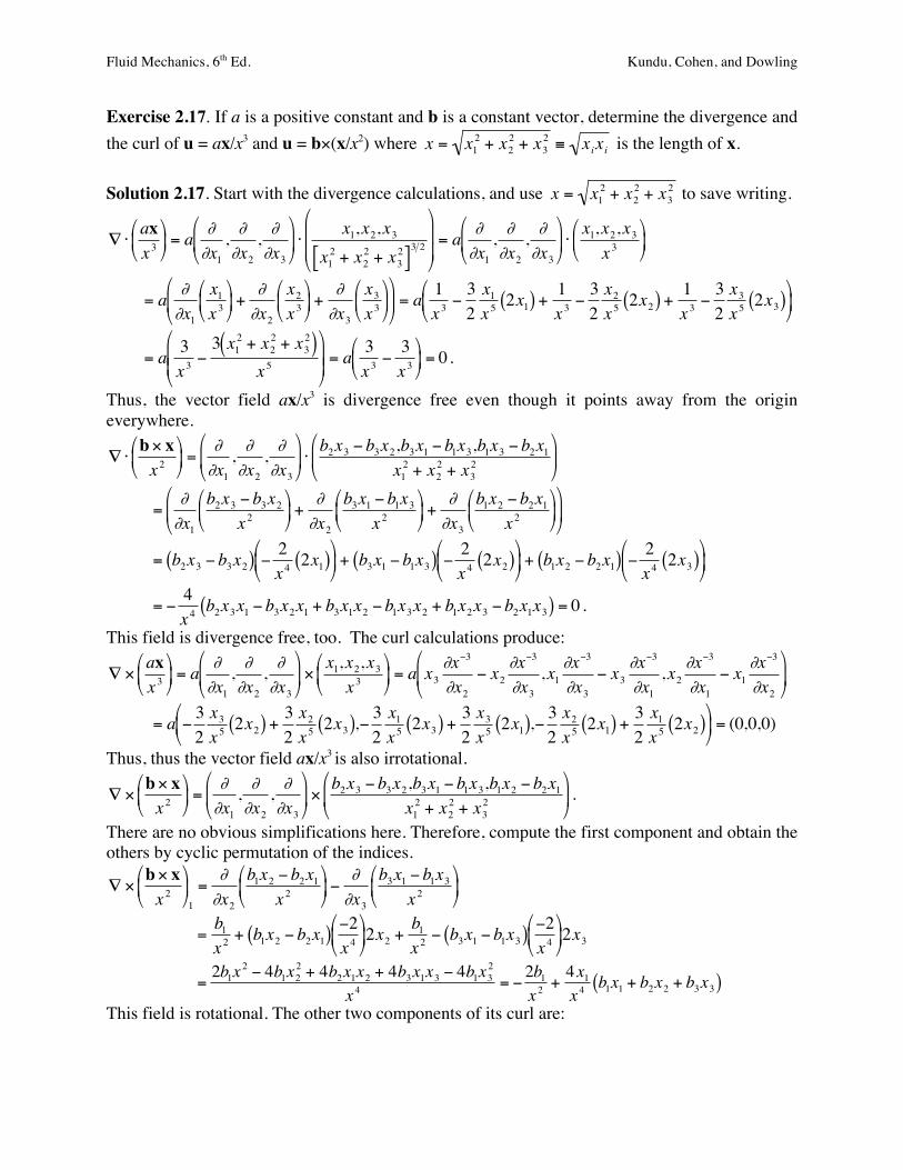
Exercise 2.17. If a is a positive constant and b is a constant vector, determine the divergence and the curl of u = ax/x3 and u = b×(x/x2) where

€

x = x12 + x2

2 + x32 ≡ xixi is the length of x.

Solution 2.17. Start with the divergence calculations, and use

€

x = x12 + x2

2 + x32 to save writing.

€

∇ ⋅axx 3

$

% &

'

( ) = a

∂∂x1, ∂∂x2

, ∂∂x3

$

% &

'

( ) ⋅

x1,x2,x3x12 + x2

2 + x32[ ]3 2

$

%

& &

'

(

) )

= a ∂∂x1, ∂∂x2

, ∂∂x3

$

% &

'

( ) ⋅

x1,x2,x3x 3

$

% &

'

( )

€

= a ∂∂x1

x1x 3#

$ %

&

' ( +

∂∂x2

x2x 3#

$ %

&

' ( +

∂∂x3

x3x 3#

$ %

&

' (

#

$ %

&

' ( = a

1x 3−32x1x 52x1( ) +

1x 3−32x2x 52x2( ) +

1x 3−32x3x 52x3( )

#

$ %

&

' (

€

= a 3x 3−3 x1

2 + x22 + x3

2( )x 5

#

$ % %

&

' ( ( = a

3x 3−3x 3

#

$ %

&

' ( = 0 .

Thus, the vector field ax/x3 is divergence free even though it points away from the origin everywhere.

€

∇ ⋅b× xx 2

%

& '

(

) * =

∂∂x1, ∂∂x2

, ∂∂x3

%

& '

(

) * ⋅

b2x3 − b3x2,b3x1 − b1x3,b1x3 − b2x1x12 + x2

2 + x32

%

& '

(

) *

€

=∂∂x1

b2x3 − b3x2x 2

$

% &

'

( ) +

∂∂x2

b3x1 − b1x3x 2

$

% &

'

( ) +

∂∂x3

b1x2 − b2x1x 2

$

% &

'

( )

$

% &

'

( )

€

= b2x3 − b3x2( ) − 2x 4

2x1( )#

$ %

&

' ( + b3x1 − b1x3( ) − 2

x 42x2( )

#

$ %

&

' ( + b1x2 − b2x1( ) − 2

x 42x3( )

#

$ %

&

' (

€

= −4x 4

b2x3x1 − b3x2x1 + b3x1x2 − b1x3x2 + b1x2x3 − b2x1x3( ) = 0 .

This field is divergence free, too. The curl calculations produce:

€

∇ ×axx 3

$

% &

'

( ) = a

∂∂x1, ∂∂x2

, ∂∂x3

$

% &

'

( ) ×

x1,x2,x3x 3

$

% &

'

( ) = a x3

∂x−3

∂x2− x2

∂x−3

∂x3,x1

∂x−3

∂x3− x3

∂x−3

∂x1,x2

∂x−3

∂x1− x1

∂x−3

∂x2

$

% &

'

( )

€

= a − 32x3x 52x2( ) +

32x2x 52x3( ),− 3

2x1x 52x3( ) +

32x3x 52x1( ),− 3

2x2x 52x1( ) +

32x1x 52x2( )

#

$ %

&

' ( = (0,0,0)

Thus, thus the vector field ax/x3 is also irrotational.

€

∇ ×b× xx 2

$

% &

'

( ) =

∂∂x1, ∂∂x2

, ∂∂x3

$

% &

'

( ) ×

b2x3 − b3x2,b3x1 − b1x3,b1x2 − b2x1x12 + x2

2 + x32

$

% &

'

( ) .

There are no obvious simplifications here. Therefore, compute the first component and obtain the others by cyclic permutation of the indices.

€

∇ ×b× xx 2

$

% &

'

( ) 1

=∂∂x2

b1x2 − b2x1x 2

$

% &

'

( ) −

∂∂x3

b3x1 − b1x3x 2

$

% &

'

( )

€

=b1x 2

+ b1x2 − b2x1( ) −2x 4#

$ %

&

' ( 2x2 +

b1x 2− b3x1 − b1x3( ) −2

x 4#

$ %

&

' ( 2x3

€

=2b1x

2 − 4b1x22 + 4b2x1x2 + 4b3x1x3 − 4b1x3

2

x 4= −

2b1x 2

+4x1x 4

b1x1 + b2x2 + b3x3( )

This field is rotational. The other two components of its curl are:


€

∇ ×b× xx 2

$

% &

'

( ) 2

= −2b2x 2

+4x2x 4

b1x1 + b2x2 + b3x3( ) ,

€

∇ ×b× xx 2

$

% &

'

( ) 3

= −2b3x 2

+4x3x 4

b1x1 + b2x2 + b3x3( ).


Exercise 2.18. Obtain the recipe for the gradient of a scalar function in cylindrical polar coordinates from the integral definition (2.32). Solution 2.18. Start from the appropriate form of (2.32),

€

∇Ψ = limV→0

1V

ΨndAA∫∫ , where Ψ is a scalar function of

position x. Here we choose a nearly rectangular volume V = (RΔϕ)(ΔR)(Δz) centered on the point x = (R, ϕ, z) with sides aligned perpendicular to the coordinate directions. Here the eϕ unit vector depends on ϕ so its direction is slightly different at ϕ ± Δϕ/2. For small Δϕ, this can be handled by keeping the linear term of a simple Taylor series:

€

eϕ[ ]ϕ ±Δϕ 2≅ eϕ ± Δϕ 2( ) ∂eϕ ∂ϕ( ) = eϕ Δϕ 2( )eR . Considering the drawing

and noting that n is an outward normal, there are six contributions to ndA:

outside =

€

R +ΔR2

#

$ %

&

' ( ΔϕΔzeR , inside =

€

− R − ΔR2

$

% &

'

( ) ΔϕΔzeR ,

close vertical side =

€

ΔRΔz −eϕ −Δϕ2eR

%

& '

(

) * , more distant vertical side =

€

ΔRΔz eϕ −Δϕ2eR

%

& '

(

) * ,

top =

€

RΔϕΔRez , and bottom =

€

−RΔϕΔRez . Here all the unit vectors are evaluated at the center of the volume. Using a two term Taylor series approximation for Ψ on each of the six surfaces, and taking the six contributions in the same order, the integral definition becomes a sum of six terms representing ΨndA.

€

∇Ψ = limΔR→0Δϕ→0Δz→0

1RΔϕΔRΔz

Ψ+ΔR2∂Ψ∂R

(

) *

+

, - R +

ΔR2

(

) *

+

, - eRΔϕΔz

.

/ 0

1

2 3 − Ψ−

ΔR2∂Ψ∂R

(

) *

+

, - R −

ΔR2

(

) *

+

, - eRΔϕΔz

.

/ 0

1

2 3 +

Ψ−Δϕ2∂Ψ∂ϕ

(

) *

+

, - −eϕ −

Δϕ2eR

(

) *

+

, - ΔRΔz

.

/ 0

1

2 3 + Ψ+

Δϕ2∂Ψ∂ϕ

(

) *

+

, - eϕ −

Δϕ2eR

(

) *

+

, - ΔRΔz

.

/ 0

1

2 3 +

Ψ+Δz2∂Ψ∂z

(

) *

+

, - ezRΔϕΔR

.

/ 0

1

2 3 − Ψ−

Δz2∂Ψ∂z

(

) *

+

, - ezRΔϕΔR

.

/ 0

1

2 3 + ...

5

6

7 7 7 7

8

7 7 7 7

9

:

7 7 7 7

;

7 7 7 7

Here the mean value theorem has been used and all listings of Ψ and its derivatives above are evaluated at the center of the volume. The largest terms inside the big {,}-brackets are proportional to ΔϕΔRΔz. The remaining higher order terms vanish when the limit is taken.

€

∇Ψ = limΔR→0Δϕ→0Δz→0

1RΔϕΔRΔz

Ψ2eR +

R2∂Ψ∂ReR

(

) * +

, - ΔϕΔRΔz − −

Ψ2eR −

R2∂Ψ∂ReR

(

) * +

, - ΔϕΔRΔz +

eϕ2∂Ψ∂ϕ

−eR2Ψ

(

) *

+

, - ΔϕΔRΔz +

eϕ2∂Ψ∂ϕ

−eR2Ψ

(

) *

+

, - ΔϕΔRΔz +

R2∂Ψ∂zez

(

) * +


R2∂Ψ∂zez

(

) * +

, - ΔϕΔRΔz + ...

/

0

1 1 1

2

1 1 1

3

4

1 1 1

5

1 1 1

€

∇Ψ =ΨReR +

∂Ψ∂ReR +

1R∂Ψ∂ϕeϕ −

ΨReR +

∂Ψ∂zez

' ( )

* + ,

= eR∂Ψ∂R

+ eϕ1R∂Ψ∂ϕ

+ ez∂Ψ∂z

x

y

z

R!

eR

e!

ez"z

"R

"!


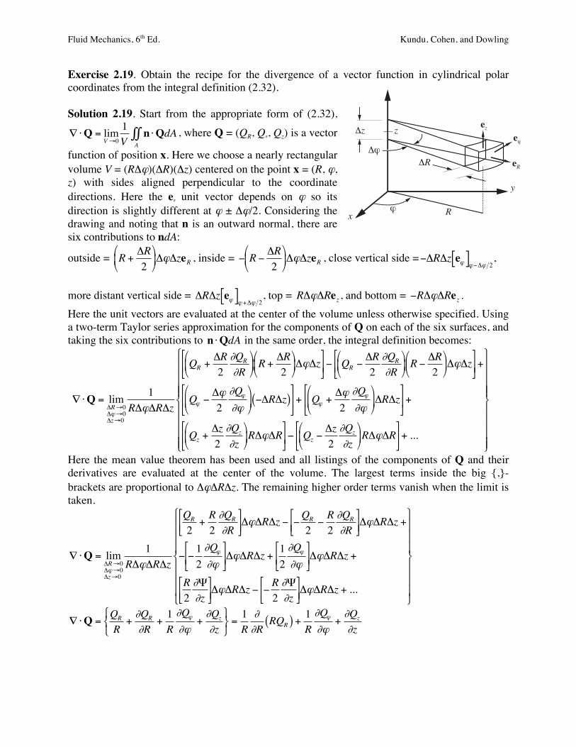
Exercise 2.19. Obtain the recipe for the divergence of a vector function in cylindrical polar coordinates from the integral definition (2.32). Solution 2.19. Start from the appropriate form of (2.32),

€

∇ ⋅Q = limV→0

1V

n ⋅QdAA∫∫ , where Q = (QR, Qϕ, Qz) is a vector

function of position x. Here we choose a nearly rectangular volume V = (RΔϕ)(ΔR)(Δz) centered on the point x = (R, ϕ, z) with sides aligned perpendicular to the coordinate directions. Here the eϕ unit vector depends on ϕ so its direction is slightly different at ϕ ± Δϕ/2. Considering the drawing and noting that n is an outward normal, there are six contributions to ndA:

outside =

€

R +ΔR2

#

$ %

&

' ( ΔϕΔzeR , inside =

€

− R − ΔR2

$

% &

'

( ) ΔϕΔzeR , close vertical side =

€

−ΔRΔz eϕ[ ]ϕ−Δϕ 2,

more distant vertical side =

€

ΔRΔz eϕ[ ]ϕ +Δϕ 2, top =

€

RΔϕΔRez , and bottom =

€

−RΔϕΔRez . Here the unit vectors are evaluated at the center of the volume unless otherwise specified. Using a two-term Taylor series approximation for the components of Q on each of the six surfaces, and taking the six contributions to

€

n ⋅QdA in the same order, the integral definition becomes:

€

∇ ⋅Q = limΔR→0Δϕ→0Δz→0

1RΔϕΔRΔz

QR +ΔR2∂QR

∂R(

) *

+

, - R +

ΔR2

(

) *

+

, - ΔϕΔz

.

/ 0

1

2 3 − QR −

ΔR2∂QR

∂R(

) *

+

, - R −

ΔR2

(

) *

+

, - ΔϕΔz

.

/ 0

1

2 3 +

Qϕ −Δϕ2∂Qϕ

∂ϕ

(

) *

+

, - −ΔRΔz( )

.

/ 0

1

2 3 + Qϕ +

Δϕ2∂Qϕ

∂ϕ

(

) *

+

, - ΔRΔz

.

/ 0

1

2 3 +

Qz +Δz2∂Qz

∂z(

) *

+

, - RΔϕΔR

.

/ 0

1

2 3 − Qz −

Δz2∂Qz

∂z(

) *

+

, - RΔϕΔR

.

/ 0

1

2 3 + ...

5

6

7 7 7 7

8

7 7 7 7

9

:

7 7 7 7

;

7 7 7 7

Here the mean value theorem has been used and all listings of the components of Q and their derivatives are evaluated at the center of the volume. The largest terms inside the big {,}-brackets are proportional to ΔϕΔRΔz. The remaining higher order terms vanish when the limit is taken.

€

∇ ⋅Q = limΔR→0Δϕ→0Δz→0

1RΔϕΔRΔz

QR

2+R2∂QR

∂R(

) * +


QR

2−R2∂QR

∂R(

) * +

, - ΔϕΔRΔz +

− −12∂Qϕ

∂ϕ

(

) *

+

, - ΔϕΔRΔz +

12∂Qϕ

∂ϕ

(

) *

+

, - ΔϕΔRΔz +

R2∂Ψ∂z

(

) * +


R2∂Ψ∂z

(

) * +

, - ΔϕΔRΔz + ...

0

1

2 2 2

3

2 2 2

4

5

2 2 2

6

2 2 2

€

∇ ⋅Q =QR

R+∂QR

∂R+1R∂Qϕ

∂ϕ+∂Qz

∂z& ' (

) * +

=1R∂∂R

RQR( ) +1R∂Qϕ

∂ϕ+∂Qz

∂z

x

y

z

R!

eR

e!

ez"z

"R

"!


Exercise 2.20. Obtain the recipe for the divergence of a vector function in spherical polar coordinates from the integral definition (2.32). Solution 2.20. Start from the appropriate

form of (2.32),

€

∇ ⋅Q = limV→0

1V

n ⋅QdAA∫∫ ,

where Q = (Qr, Qθ, Qϕ) is a vector function of position x. Here we choose a nearly rectangular volume V = (rΔθ)(rsinθΔϕ)(Δr) centered on the point x = (r, θ, ϕ) with sides aligned perpendicular to the coordinate directions. Here the unit vectors depend on θ and ϕ so directions are slightly different at θ ± Δθ/2, and ϕ ± Δϕ/2. Considering the drawing and noting that n is an outward normal, there are six contributions to ndA:

outside =

€

r +Δr2

#

$ %

&

' ( Δθ r +

Δr2

#

$ %

&

' ( sinθΔϕ er( ) , inside =

€

r − Δr2

$

% &

'

( ) Δθ r − Δr

2$

% &

'

( ) sinθΔϕ −er( ),

bottom =

€

rsin θ + Δθ 2( )ΔϕΔr[ ] eθ( )θ +Δθ 2 , top =

€

rsin θ −Δθ 2( )ΔϕΔr[ ] −eθ( )θ −Δθ 2 ,

close vertical side =

€

rΔθΔr −eϕ( )ϕ−Δϕ 2, and more distant vertical side =

€

rΔθΔr +eϕ( )ϕ +Δϕ 2.

Here the unit vectors are evaluated at the center of the volume unless otherwise specified. Using a two-term Taylor series approximation for the corresponding components of Q on each of the six surfaces produces:

outside:

€

Qr +Δr2∂Qr

∂r$

% &

'

( ) er , inside:

€

Qr −Δr2∂Qr

∂r%

& '

(

) * er , bottom:

€

Qθ +Δθ2∂Qθ

∂θ

%

& '

(

) * eθ( )θ +Δθ 2,

top:

€

Qθ −Δθ2∂Qθ

∂θ

&

' (

)

* + eθ( )θ −Δθ 2 , close vertical side :

€

Qϕ −Δϕ2∂Qϕ

∂ϕ

&

' (

)

* + −eϕ( )ϕ−Δϕ 2

, and

more distant vertical side :

€

Qϕ +Δϕ2∂Qϕ

∂ϕ

%

& '

(

) * eϕ( )ϕ +Δϕ 2

.

Collecting and summing the six contributions to

€

n ⋅QdA , the integral definition becomes:

€

∇ ⋅Q = limΔr→0Δθ →0Δϕ→0

1(rΔθ)(rsinθΔϕ)Δr

×

Qr +Δr2∂Qr

∂r*

+ ,

-

. / Δθ r +

Δr2

*

+ ,

-

. / 2

sinθΔϕ0

1 2

3

4 5 − Qr −

Δr2∂Qr

∂r*

+ ,

-

. / Δθ r − Δr

2*

+ ,

-

. / 2

sinθΔϕ0

1 2

3

4 5

+ Qθ +Δθ2∂Qθ

∂θ

*

+ ,

-

. / rsin θ +

Δθ2

*

+ ,

-

. / ΔϕΔr

0

1 2

3

4 5 − Qθ −

Δθ2∂Qθ

∂θ

*

+ ,

-

. / rsin θ −

Δθ2

*

+ ,

-

. / ΔϕΔr

0

1 2

3

4 5

− Qϕ −Δϕ2∂Qϕ

∂ϕ

*

+ ,

-

. / rΔθΔr

0

1 2

3

4 5 + Qϕ +

Δϕ2∂Qϕ

∂ϕ

*

+ ,

-

. / rΔθΔr

0

1 2

3

4 5 + ...

7

8

9 9 9 9

:

9 9 9 9

;

<

9 9 9 9

=

9 9 9 9

x

y

z

!

er

e!

e"

#r

#!

"

#"

rsin"


The largest terms inside the big {,}-brackets are proportional to ΔθΔϕΔr. The remaining higher order terms vanish when the limit is taken.

€

∇ ⋅Q = limΔr→0Δθ →0Δϕ→0

1(rΔθ)(rsinθΔϕ)Δr

×

r2 ∂Qr

∂r+ 2rQr

*

+ , -

. / Δθ sinθΔϕΔr

+ sinθ ∂Qθ

∂θ+ cosθQθ

*

+ , -

. / rΔθΔϕΔr

+∂Qϕ

∂ϕ

*

+ ,

-

. / rΔθΔϕΔr + ...

0

1

2 2 2

3

2 2 2

4

5

2 2 2

6

2 2 2

Cancel the common factors and take the limit, to find:

€

∇ ⋅Q =1

(r)(rsinθ)× r2 ∂Qr

∂r+ 2rQr

'

( ) *

+ , sinθ + sinθ ∂Qθ

∂θ+ cosθQθ

'

( ) *

+ , r +

∂Qϕ

∂ϕ

'

( )

*

+ , r

. / 0

1 2 3

€

=1

r2 sinθ×

∂∂r

r2Qr( )sinθ + r ∂∂θ

sinθQθ( ) + r∂Qϕ

∂ϕ

& ' (

) * +

€

=1r2

∂∂r

r2Qr( ) +1

rsinθ∂∂θ

sinθQθ( ) +1

rsinθ∂Qϕ

∂ϕ


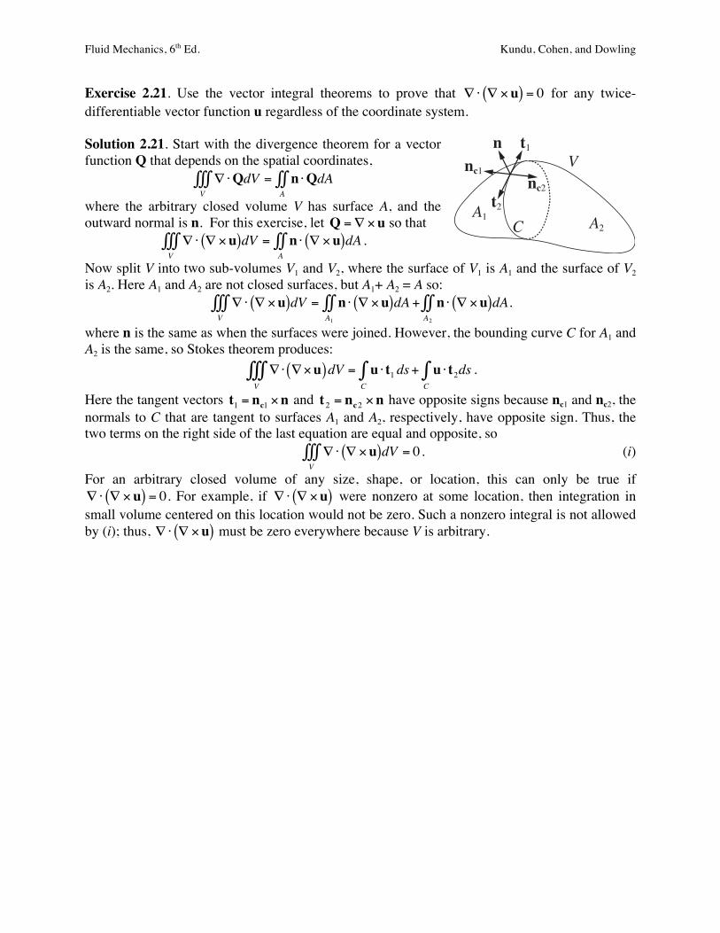
Exercise 2.21. Use the vector integral theorems to prove that

€

∇ ⋅ ∇ ×u( ) = 0 for any twice-differentiable vector function u regardless of the coordinate system. Solution 2.21. Start with the divergence theorem for a vector function Q that depends on the spatial coordinates,

€

∇ ⋅QdV = n ⋅QdAA∫∫

V∫∫∫

where the arbitrary closed volume V has surface A, and the outward normal is n. For this exercise, let

€

Q =∇ ×u so that

€

∇ ⋅ ∇ ×u( )dV = n ⋅ ∇ ×u( )dAA∫∫

V∫∫∫ .

Now split V into two sub-volumes V1 and V2, where the surface of V1 is A1 and the surface of V2 is A2. Here A1 and A2 are not closed surfaces, but A1+ A2 = A so:

€

∇ ⋅ ∇ ×u( )dV = n ⋅ ∇ ×u( )dA +A1

∫∫V∫∫∫ n ⋅ ∇ ×u( )dA

A2

∫∫ .

where n is the same as when the surfaces were joined. However, the bounding curve C for A1 and A2 is the same, so Stokes theorem produces:

∇⋅ ∇×u( )dV = u ⋅ t1C∫ ds

V∫∫∫ + u ⋅ t2

C∫ ds .

Here the tangent vectors

€

t1 = nc1 ×n and

€

t2 = nc2 ×n have opposite signs because nc1 and nc2, the normals to C that are tangent to surfaces A1 and A2, respectively, have opposite sign. Thus, the two terms on the right side of the last equation are equal and opposite, so

€

∇ ⋅ ∇ ×u( )dVV∫∫∫ = 0 . (i)

For an arbitrary closed volume of any size, shape, or location, this can only be true if

€

∇ ⋅ ∇ ×u( ) = 0. For example, if

€

∇ ⋅ ∇ ×u( ) were nonzero at some location, then integration in small volume centered on this location would not be zero. Such a nonzero integral is not allowed by (i); thus,

€

∇ ⋅ ∇ ×u( ) must be zero everywhere because V is arbitrary.

A1A2

t1

t2

nc1

nc2

C

n

V


Exercise 2.22. Use Stokes’ theorem to prove that

€

∇ × ∇φ( ) = 0 for any single-valued twice-differentiable scalar φ regardless of the coordinate system. Solution 2.22. From (2.34) Stokes Theorem is:

€

∇ ×u( )A∫∫ ⋅ndA = u

C∫ ⋅ tds.

Let

€

u =∇φ , and note that

€

∇φ ⋅ tds = ∂φ ∂s( )ds = dφ because the t vector points along the contour C that has path increment ds. Therefore:

€

∇ × ∇φ[ ]( )A∫∫ ⋅ndA = ∇φ

C∫ ⋅ tds = dφ = 0

C∫ , (ii)

where the final equality holds for integration on a closed contour of a single-valued function φ. For an arbitrary surface A of any size, shape, orientation, or location, this can only be true if ∇× ∇φ( ) = 0 . For example, if ∇× ∇φ( ) = 0 were nonzero at some location, then an area integration in a small region centered on this location would not be zero. Such a nonzero integral is not allowed by (ii); thus, ∇× ∇φ( ) = 0 must be zero everywhere because A is arbitrary.

Engineering

Fluid Mechanics Kundu Cohen 6th edition solutions Sm ch (2)